Recent Advances in Autoencoder-BasedRepresentation Learning

Michael TschannenETH Zurich

michaelt@nari.ee.ethz.ch

Olivier BachemGoogle AI, Brain Teambachem@google.com

Mario LucicGoogle AI, Brain Teamlucic@google.com

Abstract

Learning useful representations with little or no supervision is a key challenge inartificial intelligence. We provide an in-depth review of recent advances in repre-sentation learning with a focus on autoencoder-based models. To organize theseresults we make use of meta-priors believed useful for downstream tasks, such asdisentanglement and hierarchical organization of features. In particular, we un-cover three main mechanisms to enforce such properties, namely (i) regularizingthe (approximate or aggregate) posterior distribution, (ii) factorizing the encod-ing and decoding distribution, or (iii) introducing a structured prior distribution.While there are some promising results, implicit or explicit supervision remainsa key enabler and all current methods use strong inductive biases and modelingassumptions. Finally, we provide an analysis of autoencoder-based representationlearning through the lens of rate-distortion theory and identify a clear tradeoff be-tween the amount of prior knowledge available about the downstream tasks, andhow useful the representation is for this task.

1 Introduction

The ability to learn useful representations of data with little or no supervision is a key challengetowards applying artificial intelligence to the vast amounts of unlabelled data collected in the world.While it is clear that the usefulness of a representation learned on data heavily depends on the endtask which it is to be used for, one could imagine that there exists properties of representationswhich are useful for many real-world tasks simultaneously. In a seminal paper on representationlearning Bengio et al. [1] proposed such a set of meta-priors. The meta-priors are derived fromgeneral assumptions about the world such as the hierarchical organization or disentanglement ofexplanatory factors, the possibility of semi-supervised learning, the concentration of data on low-dimensional manifolds, clusterability, and temporal and spatial coherence.

Recently, a variety of (unsupervised) representation learning algorithms have been proposed basedon the idea of autoencoding where the goal is to learn a mapping from high-dimensional observa-tions to a lower-dimensional representation space such that the original observations can be recon-structed (approximately) from the lower-dimensional representation. While these approaches havevarying motivations and design choices, we argue that essentially all of the methods reviewed in thispaper implicitly or explicitly have at their core at least one of the meta-priors from Bengio et al. [1].

Given the unsupervised nature of the upstream representation learning task, the characteristics ofthe meta-priors enforced in the representation learning step determine how useful the resulting rep-resentation is for the real-world end task. Hence, it is critical to understand which meta-priors aretargeted by which models and which generic techniques are useful to enforce a given meta-prior. Inthis paper, we provide a unified view which encompasses the majority of proposed models and relatethem to the meta-priors proposed by Bengio et al. [1]. We summarize the recent work focusing onthe meta-priors in Table 1.

Third workshop on Bayesian Deep Learning (NeurIPS 2018), Montreal, Canada.

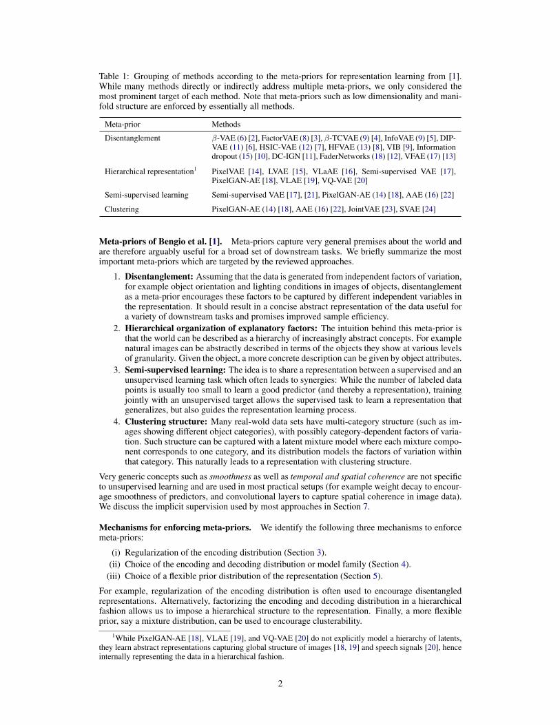
Table 1: Grouping of methods according to the meta-priors for representation learning from [1].While many methods directly or indirectly address multiple meta-priors, we only considered themost prominent target of each method. Note that meta-priors such as low dimensionality and mani-fold structure are enforced by essentially all methods.

Meta-prior Methods

Disentanglement β-VAE (6) [2], FactorVAE (8) [3], β-TCVAE (9) [4], InfoVAE (9) [5], DIP-VAE (11) [6], HSIC-VAE (12) [7], HFVAE (13) [8], VIB [9], Informationdropout (15) [10], DC-IGN [11], FaderNetworks (18) [12], VFAE (17) [13]

Hierarchical representation1 PixelVAE [14], LVAE [15], VLaAE [16], Semi-supervised VAE [17],PixelGAN-AE [18], VLAE [19], VQ-VAE [20]

Semi-supervised learning Semi-supervised VAE [17], [21], PixelGAN-AE (14) [18], AAE (16) [22]

Clustering PixelGAN-AE (14) [18], AAE (16) [22], JointVAE [23], SVAE [24]

Meta-priors of Bengio et al. [1]. Meta-priors capture very general premises about the world andare therefore arguably useful for a broad set of downstream tasks. We briefly summarize the mostimportant meta-priors which are targeted by the reviewed approaches.

1. Disentanglement: Assuming that the data is generated from independent factors of variation,for example object orientation and lighting conditions in images of objects, disentanglementas a meta-prior encourages these factors to be captured by different independent variables inthe representation. It should result in a concise abstract representation of the data useful fora variety of downstream tasks and promises improved sample efficiency.

2. Hierarchical organization of explanatory factors: The intuition behind this meta-prior isthat the world can be described as a hierarchy of increasingly abstract concepts. For examplenatural images can be abstractly described in terms of the objects they show at various levelsof granularity. Given the object, a more concrete description can be given by object attributes.

3. Semi-supervised learning: The idea is to share a representation between a supervised and anunsupervised learning task which often leads to synergies: While the number of labeled datapoints is usually too small to learn a good predictor (and thereby a representation), trainingjointly with an unsupervised target allows the supervised task to learn a representation thatgeneralizes, but also guides the representation learning process.

4. Clustering structure: Many real-wold data sets have multi-category structure (such as im-ages showing different object categories), with possibly category-dependent factors of varia-tion. Such structure can be captured with a latent mixture model where each mixture compo-nent corresponds to one category, and its distribution models the factors of variation withinthat category. This naturally leads to a representation with clustering structure.

Very generic concepts such as smoothness as well as temporal and spatial coherence are not specificto unsupervised learning and are used in most practical setups (for example weight decay to encour-age smoothness of predictors, and convolutional layers to capture spatial coherence in image data).We discuss the implicit supervision used by most approaches in Section 7.

Mechanisms for enforcing meta-priors. We identify the following three mechanisms to enforcemeta-priors:

(i) Regularization of the encoding distribution (Section 3).(ii) Choice of the encoding and decoding distribution or model family (Section 4).

(iii) Choice of a flexible prior distribution of the representation (Section 5).

For example, regularization of the encoding distribution is often used to encourage disentangledrepresentations. Alternatively, factorizing the encoding and decoding distribution in a hierarchicalfashion allows us to impose a hierarchical structure to the representation. Finally, a more flexibleprior, say a mixture distribution, can be used to encourage clusterability.

1While PixelGAN-AE [18], VLAE [19], and VQ-VAE [20] do not explicitly model a hierarchy of latents,they learn abstract representations capturing global structure of images [18, 19] and speech signals [20], henceinternally representing the data in a hierarchical fashion.

2

x(i) x(i)

z(i)µ

�

q�(z|x) p✓(x|z)

p(z)

encoder decoder

prior

x(i) x(i)

z(i)µ

�

q�(z|x) p✓(x|z)

p1(z) p2(z)

x(i)

x(i)

p(z)

z(i)1 z(i)2

µ1

µ2

�2

�1

q�(z1, z2|x)

p✓(x|z1, z2)

PixelCNN

or

code

(a) Variational Autoencoder (VAE) framework.

(b) Samples from a trained VAE.

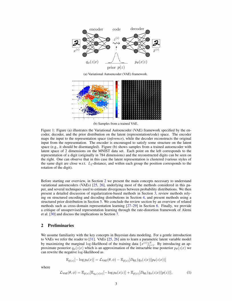
Figure 1: Figure (a) illustrates the Variational Autoencoder (VAE) framework specified by the en-coder, decoder, and the prior distribution on the latent (representation/code) space. The encodermaps the input to the representation space (inference), while the decoder reconstructs the originalinput from the representation. The encoder is encouraged to satisfy some structure on the latentspace (e.g., it should be disentangled). Figure (b) shows samples from a trained autoencoder withlatent space of 2 dimensions on the MNIST data set. Each point on the left corresponds to therepresentation of a digit (originally in 784 dimensions) and the reconstructed digits can be seen onthe right. One can observe that in this case the latent representation is clustered (various styles ofthe same digit are close w.r.t. L2-distance, and within each group the position corresponds to therotation of the digit).

Before starting our overview, in Section 2 we present the main concepts necessary to understandvariational autoencoders (VAEs) [25, 26], underlying most of the methods considered in this pa-per, and several techniques used to estimate divergences between probability distributions. We thenpresent a detailed discussion of regularization-based methods in Section 3, review methods rely-ing on structured encoding and decoding distributions in Section 4, and present methods using astructured prior distribution in Section 5. We conclude the review section by an overview of relatedmethods such as cross-domain representation learning [27–29] in Section 6. Finally, we providea critique of unsupervised representation learning through the rate-distortion framework of Alemiet al. [30] and discuss the implications in Section 7.

2 Preliminaries

We assume familiarity with the key concepts in Bayesian data modeling. For a gentle introductionto VAEs we refer the reader to [31]. VAEs [25, 26] aim to learn a parametric latent variable modelby maximizing the marginal log-likelihood of the training data {x(i)}Ni=1. By introducing an ap-proximate posterior qφ(z|x) which is an approximation of the intractable true posterior pθ(z|x) wecan rewrite the negative log-likelihood as

Ep(x)[− log pθ(x)] = LVAE(θ, φ)− Ep(x)[DKL(qφ(z|x)‖pθ(z|x))]

whereLVAE(θ, φ) = Ep(x)[Eqφ(z|x)[− log pθ(x|z)] + Ep(x)[DKL(qφ(z|x)‖p(z))], (1)

3

generator

discriminatorpy

px

c = 1

c = 0noise

(a) The main idea behind GANs.

feature mapping '

MMD(px, py)

px

py

(b) The main idea behind MMD.

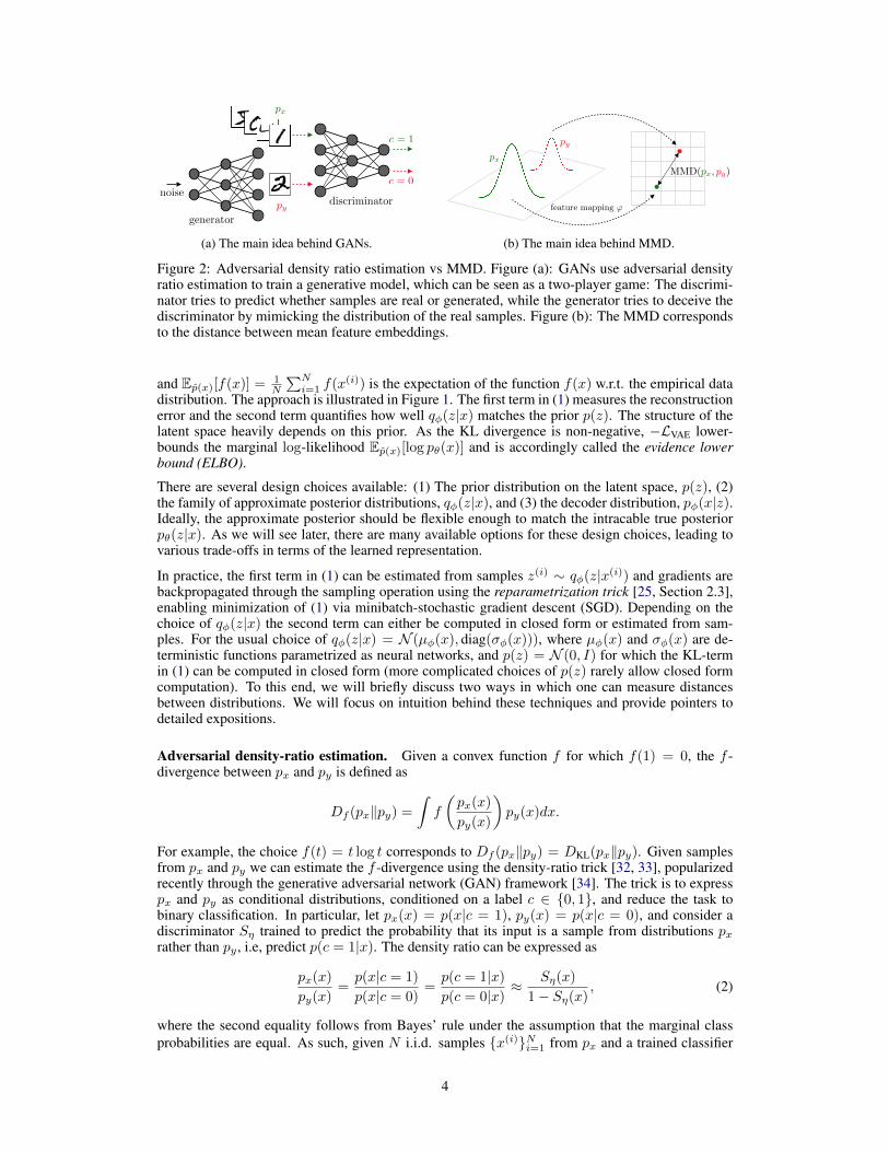
Figure 2: Adversarial density ratio estimation vs MMD. Figure (a): GANs use adversarial densityratio estimation to train a generative model, which can be seen as a two-player game: The discrimi-nator tries to predict whether samples are real or generated, while the generator tries to deceive thediscriminator by mimicking the distribution of the real samples. Figure (b): The MMD correspondsto the distance between mean feature embeddings.

and Ep(x)[f(x)] = 1N

∑Ni=1 f(x

(i)) is the expectation of the function f(x) w.r.t. the empirical datadistribution. The approach is illustrated in Figure 1. The first term in (1) measures the reconstructionerror and the second term quantifies how well qφ(z|x) matches the prior p(z). The structure of thelatent space heavily depends on this prior. As the KL divergence is non-negative, −LVAE lower-bounds the marginal log-likelihood Ep(x)[log pθ(x)] and is accordingly called the evidence lowerbound (ELBO).

There are several design choices available: (1) The prior distribution on the latent space, p(z), (2)the family of approximate posterior distributions, qφ(z|x), and (3) the decoder distribution, pφ(x|z).Ideally, the approximate posterior should be flexible enough to match the intracable true posteriorpθ(z|x). As we will see later, there are many available options for these design choices, leading tovarious trade-offs in terms of the learned representation.

In practice, the first term in (1) can be estimated from samples z(i) ∼ qφ(z|x(i)) and gradients arebackpropagated through the sampling operation using the reparametrization trick [25, Section 2.3],enabling minimization of (1) via minibatch-stochastic gradient descent (SGD). Depending on thechoice of qφ(z|x) the second term can either be computed in closed form or estimated from sam-ples. For the usual choice of qφ(z|x) = N (µφ(x), diag(σφ(x))), where µφ(x) and σφ(x) are de-terministic functions parametrized as neural networks, and p(z) = N (0, I) for which the KL-termin (1) can be computed in closed form (more complicated choices of p(z) rarely allow closed formcomputation). To this end, we will briefly discuss two ways in which one can measure distancesbetween distributions. We will focus on intuition behind these techniques and provide pointers todetailed expositions.

Adversarial density-ratio estimation. Given a convex function f for which f(1) = 0, the f -divergence between px and py is defined as

Df (px‖py) =∫f

(px(x)

py(x)

)py(x)dx.

For example, the choice f(t) = t log t corresponds to Df (px‖py) = DKL(px‖py). Given samplesfrom px and py we can estimate the f -divergence using the density-ratio trick [32, 33], popularizedrecently through the generative adversarial network (GAN) framework [34]. The trick is to expresspx and py as conditional distributions, conditioned on a label c ∈ {0, 1}, and reduce the task tobinary classification. In particular, let px(x) = p(x|c = 1), py(x) = p(x|c = 0), and consider adiscriminator Sη trained to predict the probability that its input is a sample from distributions pxrather than py , i.e, predict p(c = 1|x). The density ratio can be expressed as

px(x)

py(x)=p(x|c = 1)

p(x|c = 0)=p(c = 1|x)p(c = 0|x) ≈

Sη(x)

1− Sη(x), (2)

where the second equality follows from Bayes’ rule under the assumption that the marginal classprobabilities are equal. As such, given N i.i.d. samples {x(i)}Ni=1 from px and a trained classifier

4

Sη one can estimate the KL-divergence by simply computing

DKL(px‖py) ≈1

N

N∑i=1

log

(Sη(x

(i))

1− Sη(x(i))

).

As a practical alternative, some approaches replace the KL term in (1) with an arbitrary divergence(e.g., maximum mean discrepancy). Note, however, that the resulting objective does not necessarilylower-bound the marginal log-likelihood of the data.

Maximum mean discrepancy (MMD) [35]. Intuitively, the distances between distributions arecomputed as distances between mean embeddings of features as illustrated in Figure 2b. Moreformally, let k : X → X be a continuous, bounded, positive semi-definite kernel and H be thecorresponding reproducing kernel Hilbert space, induced by the feature mapping ϕ : X → H. Then,the MMD of distributions px(x) and py(y) is

MMD(px, py) = ‖Ex∼px [ϕ(x)]− Ey∼py [ϕ(y)]‖2H. (3)

For example, setting X = H = Rd and ϕ(x) = x, MMD reduces to the difference betweenthe means, i.e., MMD(px, py) = ‖µpx − µpy‖22. By choosing an appropriate mapping ϕ one canestimate the divergence in terms of higher order moments of the distribution.

MMD vs f -divergences in practice. The MMD is known to work particularly well with mul-tivariate standard normal distributions. It requires a sample size roughly on the order of the datadimensionality. When used as a regularizer (see Section 3), it generally allows for stable optimiza-tion. A disadvantage is that it requires selection of the kernel k and its bandwidth parameter. Incontrast, f -divergence estimators based on the density-ratio trick can in principle handle more com-plex distributions than MMD. However, in practice they require adversarial training which currentlysuffers from optimization issues. For more details consult [36, Section 3].

Deterministic autoencoders. Some of the methods we review rely on deterministic encoders anddecoders. We denote by Dθ and Eφ the deterministic encoder and decoder, respectively. A popularobjective for training an autoencoder is to minimize the L2-loss, namely

LAE(θ, φ) =1

2Ep(x)[‖x−Dθ(Eφ(x))‖22]. (4)

If Eφ and Dθ are linear maps and the representation z is lower-dimensional than x, (4) correspondsto principal component analysis (PCA), which leads to z with decorrelated entries. Furthermore,we obtain (4) by removing the DKL-term from LVAE in (1) and using a deterministic encodingdistribution qφ(z|x) and a Gaussian decoding distribution pθ(x|z). Therefore, the major differencebetween LAE and LVAE is that LAE does not enforce a prior distribution on the latent space (e.g.,through a DKL-term), and minimizing LAE hence does not yield a generative model.

3 Regularization-based methods

A classic approach to enforce some meta-prior on the latent representations z ∼ qφ(z|x) is toaugment LVAE with regularizers that act on the approximate posterior qφ(z|x) and/or the aggregate(approximate) posterior qφ(z) = Ep(x)[qφ(z|x)] = 1

N

∑Ni=1 qφ(z|x(i)). The vast majority of recent

work can be subsumed into an objective of the form

LVAE(θ, φ) + λ1Ep(x)[R1(qφ(z|x))] + λ2R2(qφ(z)), (5)

where R1 and R2 are regularizers and λ1, λ2 > 0 the corresponding weights. Firstly, we note a keydifference between regularizers R1 and R2 is that the latter depends on the entire data set throughqφ(z). In principle, this prevents the use of mini-batch SGD to solve (5). In practice, however,one can often obtain good mini-batch-based estimates of R2(qφ(z)). Secondly, the regularizersbias LVAE towards a looser (larger) upper bound on the negative marginal log-likelihood. From thisperspective it is not surprising that many approaches yield a lower reconstruction quality (whichtypically corresponds to a larger negative log-likelihood). For deterministic autoencoders, there isno such concept as an aggregated posterior, so we consider objectives of the form LAE(θ, φ) +λ1Ep(x)[R1(E(x))].

5

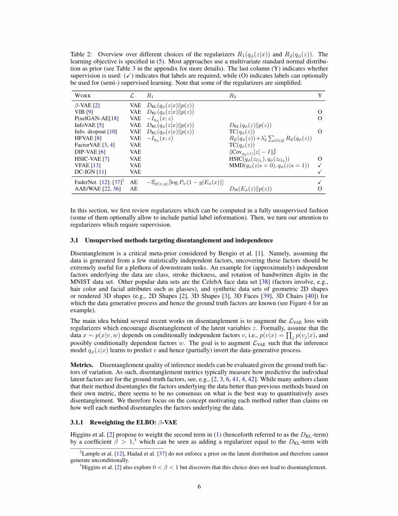
Table 2: Overview over different choices of the regularizers R1(qφ(z|x)) and R2(qφ(z)). Thelearning objective is specified in (5). Most approaches use a multivariate standard normal distribu-tion as prior (see Table 3 in the appendix for more details). The last column (Y) indicates whethersupervision is used: (X) indicates that labels are required, while (O) indicates labels can optionallybe used for (semi-) supervised learning. Note that some of the regularizers are simplified.

WORK L· R1 R2 Y

β-VAE [2] VAE DKL(qφ(z|x)‖p(z))VIB [9] VAE DKL(qφ(z|x)‖p(z)) OPixelGAN-AE[18] VAE −Iqφ(x; z) OInfoVAE [5] VAE DKL(qφ(z|x)‖p(z)) DKL(qφ(z)‖p(z))Info. dropout [10] VAE DKL(qφ(z|x)‖p(z)) TC(qφ(z)) OHFVAE [8] VAE −Iqφ(x; z) RG(qφ(z))+λ

′2

∑G∈G RG(qφ(z))

FactorVAE [3, 4] VAE TC(qφ(z))DIP-VAE [6] VAE ‖Covqφ(z)[z]− I‖

2F

HSIC-VAE [7] VAE HSIC(qφ(zG1), qφ(zG2)) OVFAE [13] VAE MMD(qφ(z|s = 0), qφ(z|s = 1)) XDC-IGN [11] VAE XFaderNet. [12]; [37]2 AE −Ep(x,y)[logPψ(1− y|Eφ(x))] XAAE/WAE [22, 36] AE DJS(Eφ(z)‖p(z)) O

In this section, we first review regularizers which can be computed in a fully unsupervised fashion(some of them optionally allow to include partial label information). Then, we turn our attention toregularizers which require supervision.

3.1 Unsupervised methods targeting disentanglement and independence

Disentanglement is a critical meta-prior considered by Bengio et al. [1]. Namely, assuming thedata is generated from a few statistically independent factors, uncovering those factors should beextremely useful for a plethora of downstream tasks. An example for (approximately) independentfactors underlying the data are class, stroke thickness, and rotation of handwritten digits in theMNIST data set. Other popular data sets are the CelebA face data set [38] (factors involve, e.g.,hair color and facial attributes such as glasses), and synthetic data sets of geometric 2D shapesor rendered 3D shapes (e.g., 2D Shapes [2], 3D Shapes [3], 3D Faces [39], 3D Chairs [40]) forwhich the data generative process and hence the ground truth factors are known (see Figure 4 for anexample).

The main idea behind several recent works on disentanglement is to augment the LVAE loss withregularizers which encourage disentanglement of the latent variables z. Formally, assume that thedata x ∼ p(x|v, w) depends on conditionally independent factors v, i.e., p(v|x) = ∏j p(vj |x), andpossibly conditionally dependent factors w. The goal is to augment LVAE such that the inferencemodel qφ(z|x) learns to predict v and hence (partially) invert the data-generative process.

Metrics. Disentanglement quality of inference models can be evaluated given the ground truth fac-tors of variation. As such, disentanglement metrics typically measure how predictive the individuallatent factors are for the ground-truth factors, see, e.g., [2, 3, 6, 41, 4, 42]. While many authors claimthat their method disentangles the factors underlying the data better than previous methods based ontheir own metric, there seems to be no consensus on what is the best way to quantitatively assesdisentanglement. We therefore focus on the concept motivating each method rather than claims onhow well each method disentangles the factors underlying the data.

3.1.1 Reweighting the ELBO: β-VAE

Higgins et al. [2] propose to weight the second term in (1) (henceforth referred to as the DKL-term)by a coefficient β > 1,3 which can be seen as adding a regularizer equal to the DKL-term with

2Lample et al. [12], Hadad et al. [37] do not enforce a prior on the latent distribution and therefore cannotgenerate unconditionally.

3Higgins et al. [2] also explore 0 < β < 1 but discovers that this choice does not lead to disentanglement.

6

x qφ(z|x) pθ(x|z) x

Ep(x)[qφ(z|x)]

HSIC(qφ(zG1), qφ(zG2)) ‖Covqφ(z)[z]− I‖2F MMD(qφ(z|s = 0), qφ(z|s = 1))

TC(qφ(z)) DKL(qφ(z)‖p(z)) DJS(q(z)‖p(z)) RG(qφ(z))+λ′2

∑G∈G RG(qφ(z))

DKL(qφ(z|x)‖p(z)) −Iqφ(x; z)

Divergence-based regularizers of qφ(z) Moment-based regularizers of qφ(z)

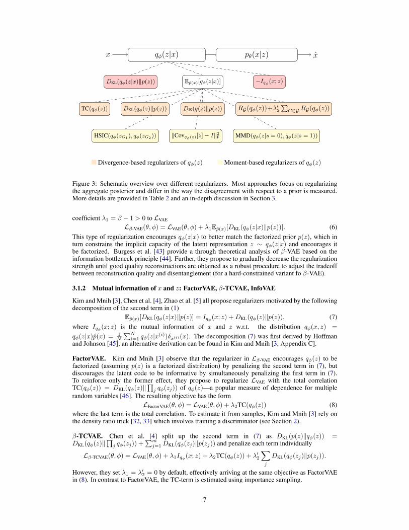
Figure 3: Schematic overview over different regularizers. Most approaches focus on regularizingthe aggregate posterior and differ in the way the disagreement with respect to a prior is measured.More details are provided in Table 2 and an in-depth discussion in Section 3.

coefficient λ1 = β − 1 > 0 to LVAE

Lβ-VAE(θ, φ) = LVAE(θ, φ) + λ1Ep(x)[DKL(qφ(z|x)‖p(z))]. (6)This type of regularization encourages qφ(z|x) to better match the factorized prior p(z), which inturn constrains the implicit capacity of the latent representation z ∼ qφ(z|x) and encourages itbe factorized. Burgess et al. [43] provide a through theoretical analysis of β-VAE based on theinformation bottleneck principle [44]. Further, they propose to gradually decrease the regularizationstrength until good quality reconstructions are obtained as a robust procedure to adjust the tradeoffbetween reconstruction quality and disentanglement (for a hard-constrained variant fo β-VAE).

3.1.2 Mutual information of x and z: FactorVAE, β-TCVAE, InfoVAE

Kim and Mnih [3], Chen et al. [4], Zhao et al. [5] all propose regularizers motivated by the followingdecomposition of the second term in (1)

Ep(x)[DKL(qφ(z|x)‖p(z)] = Iqφ(x; z) +DKL(qφ(z)‖p(z)), (7)where Iqφ(x; z) is the mutual information of x and z w.r.t. the distribution qφ(x, z) =

qφ(z|x)p(x) = 1N

∑Ni=1 qφ(z|x(i))δx(i)(x). The decomposition (7) was first derived by Hoffman

and Johnson [45]; an alternative derivation can be found in Kim and Mnih [3, Appendix C].

FactorVAE. Kim and Mnih [3] observe that the regularizer in Lβ-VAE encourages qφ(z) to befactorized (assuming p(z) is a factorized distribution) by penalizing the second term in (7), butdiscourages the latent code to be informative by simultaneously penalizing the first term in (7).To reinforce only the former effect, they propose to regularize LVAE with the total correlationTC(qφ(z)) = DKL(qφ(z)‖

∏j qφ(zj)) of qφ(z)—a popular measure of dependence for multiple

random variables [46]. The resulting objective has the formLFactorVAE(θ, φ) = LVAE(θ, φ) + λ2TC(qφ(z)) (8)

where the last term is the total correlation. To estimate it from samples, Kim and Mnih [3] rely onthe density ratio trick [32, 33] which involves training a discriminator (see Section 2).

β-TCVAE. Chen et al. [4] split up the second term in (7) as DKL(p(z)‖qφ(z)) =DKL(qφ(z)‖

∏j qφ(zj)) +

∑mj=1DKL(qφ(zj)‖p(zj)) and penalize each term individually

Lβ-TCVAE(θ, φ) = LVAE(θ, φ) + λ1Iqφ(x; z) + λ2TC(qφ(z)) + λ′2∑j

DKL(qφ(zj)‖p(zj)).

However, they set λ1 = λ′2 = 0 by default, effectively arriving at the same objective as FactorVAEin (8). In contrast to FactorVAE, the TC-term is estimated using importance sampling.

7

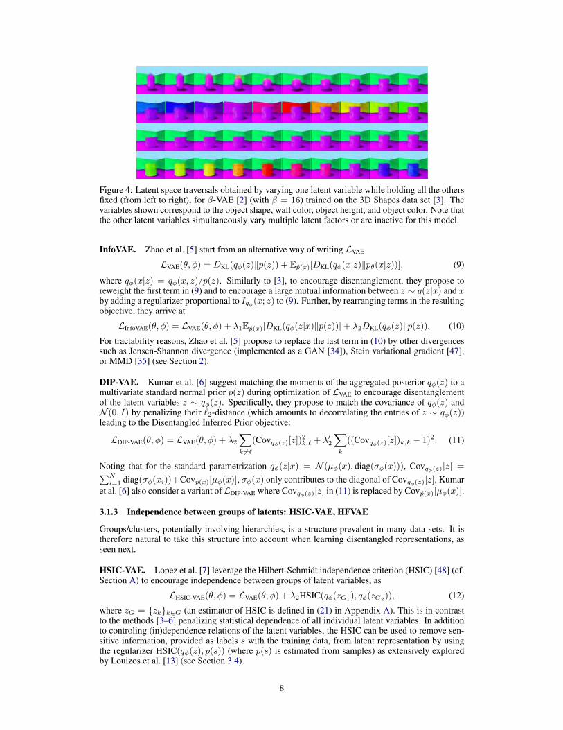
Figure 4: Latent space traversals obtained by varying one latent variable while holding all the othersfixed (from left to right), for β-VAE [2] (with β = 16) trained on the 3D Shapes data set [3]. Thevariables shown correspond to the object shape, wall color, object height, and object color. Note thatthe other latent variables simultaneously vary multiple latent factors or are inactive for this model.

InfoVAE. Zhao et al. [5] start from an alternative way of writing LVAE

LVAE(θ, φ) = DKL(qφ(z)‖p(z)) + Ep(x)[DKL(qφ(x|z)‖pθ(x|z))], (9)

where qφ(x|z) = qφ(x, z)/p(z). Similarly to [3], to encourage disentanglement, they propose toreweight the first term in (9) and to encourage a large mutual information between z ∼ q(z|x) and xby adding a regularizer proportional to Iqφ(x; z) to (9). Further, by rearranging terms in the resultingobjective, they arrive at

LInfoVAE(θ, φ) = LVAE(θ, φ) + λ1Ep(x)[DKL(qφ(z|x)‖p(z))] + λ2DKL(qφ(z)‖p(z)). (10)

For tractability reasons, Zhao et al. [5] propose to replace the last term in (10) by other divergencessuch as Jensen-Shannon divergence (implemented as a GAN [34]), Stein variational gradient [47],or MMD [35] (see Section 2).

DIP-VAE. Kumar et al. [6] suggest matching the moments of the aggregated posterior qφ(z) to amultivariate standard normal prior p(z) during optimization of LVAE to encourage disentanglementof the latent variables z ∼ qφ(z). Specifically, they propose to match the covariance of qφ(z) andN (0, I) by penalizing their `2-distance (which amounts to decorrelating the entries of z ∼ qφ(z))leading to the Disentangled Inferred Prior objective:

LDIP-VAE(θ, φ) = LVAE(θ, φ) + λ2∑k 6=`

(Covqφ(z)[z])2k,` + λ′2

∑k

((Covqφ(z)[z])k,k − 1)2. (11)

Noting that for the standard parametrization qφ(z|x) = N (µφ(x), diag(σφ(x))), Covqφ(z)[z] =∑Ni=1 diag(σφ(xi))+Covp(x)[µφ(x)], σφ(x) only contributes to the diagonal of Covqφ(z)[z], Kumar

et al. [6] also consider a variant of LDIP-VAE where Covqφ(z)[z] in (11) is replaced by Covp(x)[µφ(x)].

3.1.3 Independence between groups of latents: HSIC-VAE, HFVAE

Groups/clusters, potentially involving hierarchies, is a structure prevalent in many data sets. It istherefore natural to take this structure into account when learning disentangled representations, asseen next.

HSIC-VAE. Lopez et al. [7] leverage the Hilbert-Schmidt independence criterion (HSIC) [48] (cf.Section A) to encourage independence between groups of latent variables, as

LHSIC-VAE(θ, φ) = LVAE(θ, φ) + λ2HSIC(qφ(zG1), qφ(zG2

)), (12)

where zG = {zk}k∈G (an estimator of HSIC is defined in (21) in Appendix A). This is in contrastto the methods [3–6] penalizing statistical dependence of all individual latent variables. In additionto controling (in)dependence relations of the latent variables, the HSIC can be used to remove sen-sitive information, provided as labels s with the training data, from latent representation by usingthe regularizer HSIC(qφ(z), p(s)) (where p(s) is estimated from samples) as extensively exploredby Louizos et al. [13] (see Section 3.4).

8

HFVAE. Starting from the decomposition (7), Esmaeili et al. [8] hierarchically decompose theDKL-term in (7) into a regularization term of the dependencies between groups of latent variablesG = {Gk}nGk=1 and regularization of the dependencies between the random variables in each groupGk. Reweighting different regularization terms allows to encourage different degrees of intra andinter-group disentanglement, leading to the following objective:

LHFVAE(θ, φ) = LVAE − λ1Iqφ(x; z)

+ λ2

(−Eqφ(z)

[log

p(z)∏G∈G p(zG)

]+DKL(qφ(z)‖

∏G∈G

qφ(zG))

)+ λ′2

∑G∈G

(−Eqφ(zG)

[log

p(zG)∏k∈G p(zk)

]+DKL(qφ(zG)‖

∏k∈G

qφ(zk))

). (13)

Here, λ1 controls the mutual information between the data and latent variables, and λ2 and λ′2determine the regularization of dependencies between groups and within groups, respectively, bypenalizing the corresponding total correlation. Note that the grouping can be nested to introducedeeper hierarchies.

3.2 Preventing the latent code from being ignored: PixelGAN-AE and VIB

PixelGAN-AE. Makhzani and Frey [18] argue that, if pθ(x|z) is not too powerful (in the sensethat it cannot model the data distribution unconditionally, i.e., without using the latent code z) theterm Iqφ(x; z) in (7) and the reconstruction term in (1) have competing effects: A small mutualinformation Iqφ(x; z) makes reconstruction of x(i) from qφ(z|x(i)) challenging for pθ(x|z), leadingto a large reconstruction error. Conversely, a small reconstruction error requires the code z to beinformative and hence Iqφ(x; z) to be large. In contrast, if the decoder is powerful, e.g., a condi-tional PixelCNN [49], such that it can obtain a small reconstruction error without relying on thelatent code, the mutual information and reconstruction terms can be minimized largely independent,which prevents the latent code from being informative and hence providing a useful representation(this issue is known as the information preference property [19] and is discussed in more detail inSection 4). In this case, to encourage the code to be informative Makhzani and Frey [18] propose todrop the Iqφ(x; z) term in (7), which can again be seen as a regularizer

LPixelGAN-AE(θ, φ) = LVAE(θ, φ)− Iqφ(x; z). (14)

The DKL term remaining in (7) after removing Iqφ is approximated using a GAN. Makhzani andFrey [18] show that relying on LPixelGAN-AE a powerful PixelCNN decoder can be trained whilekeeping the latent code informative. Depending on the choice of the prior (categorical or Gaussian),the latent code picks up information of different levels of abstraction, for example the digit class andwriting style in the case of MNIST.

VIB, information dropout. Alemi et al. [9] and Achille and Soatto [10] both derive a variationalapproximation of the information bottleneck objective [10], which targets learning a compact repre-sentation z of some random variable x that is maximally informative about some random variable y.In the special case, when y = x, the approximation derived in [9] one obtains an objective equivalentto Lβ-VAE in (1) (c.f. [9, Appendix B] for a discussion), whereas doing so for [10] leads to

LInfoDrop(θ, φ) = LVAE(θ, φ) + λ1Ep(x)[DKL(qφ(z|x)‖p(z))] + λ2TC(qφ(z)). (15)

Achille and Soatto [10] derive (more) tractable expressions for (15) and establishe a connectionto dropout for particular choices of p(z) and qφ(z|x). Alemi et al. [30] propose an information-theoretic framework studying the representation learning properties of VAE-like models through arate-distortion tradeoff. This framework recovers β-VAE but allows for a more precise navigationof the feasible rate-distortion region than the latter. Alemi and Fischer [50] further generalize theframework of [9], as discussed in Section 7.

3.3 Deterministic encoders and decoders: AAE and WAE

Adversarial Autoencoders (AAEs) [22] turn a standard autoencoder into a generative model by im-posing a prior distribution p(z) on the latent variables by penalizing some statistical divergence Df

9

between p(z) and qφ(z) using a GAN. Specifically, using the negative log-likelihood as reconstruc-tion loss, the AAE objective can be written as

LAAE(θ, φ) = Ep(x)[Eqφ(z|x)[− log pθ(x|z)]] + λ2Df (q(z)‖p(z)). (16)

In all experiments in [22] encoder and decoder are taken to be deterministic, i.e., p(x|z) and q(z|x)are replaced by Dθ and Eφ, respectively, and the negative log-likelihood in (16) is replaced with thestandard autoencoder loss LAE. The advantage of implementing the regularizer λ2Df using a GANis that any p(z) we can sample from, can be matched. This is helpful to learn representations: Forexample for MNIST, enforcing a prior that involves both categorical and Gaussian latent variables isshown to disentangle discrete and continuous style information in unsupervised fashion, in the sensethat the categorical latent variables model the digit index and continuous random variables the writ-ing style. Disentanglement can be improved by leveraging (partial) label information, regularizingthe cross-entropy between the categorical latent variables and the label one-hot encodings. Partiallabel information also allows to learn a generative model for digits with a Gaussian mixture modelprior, with every mixture component corresponding to one digit index.

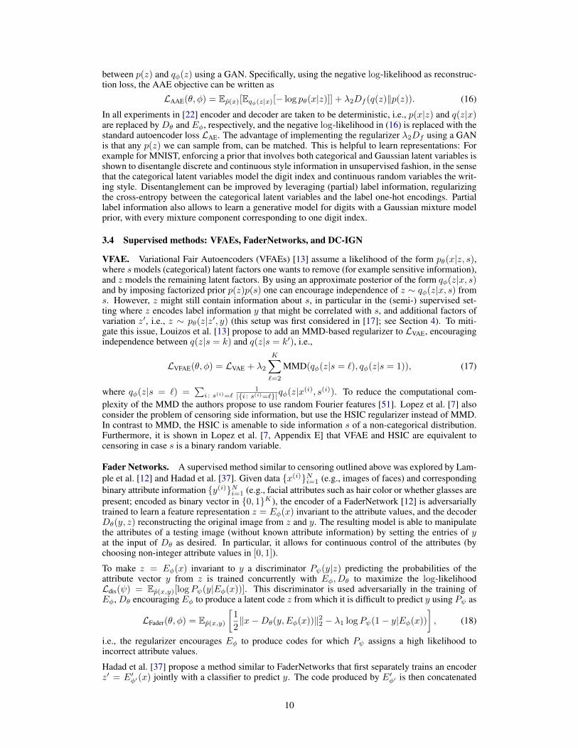
3.4 Supervised methods: VFAEs, FaderNetworks, and DC-IGN

VFAE. Variational Fair Autoencoders (VFAEs) [13] assume a likelihood of the form pθ(x|z, s),where smodels (categorical) latent factors one wants to remove (for example sensitive information),and z models the remaining latent factors. By using an approximate posterior of the form qφ(z|x, s)and by imposing factorized prior p(z)p(s) one can encourage independence of z ∼ qφ(z|x, s) froms. However, z might still contain information about s, in particular in the (semi-) supervised set-ting where z encodes label information y that might be correlated with s, and additional factors ofvariation z′, i.e., z ∼ pθ(z|z′, y) (this setup was first considered in [17]; see Section 4). To miti-gate this issue, Louizos et al. [13] propose to add an MMD-based regularizer to LVAE, encouragingindependence between q(z|s = k) and q(z|s = k′), i.e.,

LVFAE(θ, φ) = LVAE + λ2

K∑`=2

MMD(qφ(z|s = `), qφ(z|s = 1)), (17)

where qφ(z|s = `) =∑i : s(i)=`

1|{i : s(i)=`}|qφ(z|x(i), s(i)). To reduce the computational com-

plexity of the MMD the authors propose to use random Fourier features [51]. Lopez et al. [7] alsoconsider the problem of censoring side information, but use the HSIC regularizer instead of MMD.In contrast to MMD, the HSIC is amenable to side information s of a non-categorical distribution.Furthermore, it is shown in Lopez et al. [7, Appendix E] that VFAE and HSIC are equivalent tocensoring in case s is a binary random variable.

Fader Networks. A supervised method similar to censoring outlined above was explored by Lam-ple et al. [12] and Hadad et al. [37]. Given data {x(i)}Ni=1 (e.g., images of faces) and correspondingbinary attribute information {y(i)}Ni=1 (e.g., facial attributes such as hair color or whether glasses arepresent; encoded as binary vector in {0, 1}K), the encoder of a FaderNetwork [12] is adversariallytrained to learn a feature representation z = Eφ(x) invariant to the attribute values, and the decoderDθ(y, z) reconstructing the original image from z and y. The resulting model is able to manipulatethe attributes of a testing image (without known attribute information) by setting the entries of yat the input of Dθ as desired. In particular, it allows for continuous control of the attributes (bychoosing non-integer attribute values in [0, 1]).

To make z = Eφ(x) invariant to y a discriminator Pψ(y|z) predicting the probabilities of theattribute vector y from z is trained concurrently with Eφ, Dθ to maximize the log-likelihoodLdis(ψ) = Ep(x,y)[logPψ(y|Eφ(x))]. This discriminator is used adversarially in the training ofEφ, Dθ encouraging Eφ to produce a latent code z from which it is difficult to predict y using Pψ as

LFader(θ, φ) = Ep(x,y)[1

2‖x−Dθ(y,Eφ(x))‖22 − λ1 logPψ(1− y|Eφ(x))

], (18)

i.e., the regularizer encourages Eφ to produce codes for which Pψ assigns a high likelihood toincorrect attribute values.

Hadad et al. [37] propose a method similar to FaderNetworks that first separately trains an encoderz′ = E′φ′(x) jointly with a classifier to predict y. The code produced by E′φ′ is then concatenated

10

x(i) x(i)

z(i)µ

�

q�(z|x) p✓(x|z)

p(z)

encoder decoder

prior

x(i) x(i)

z(i)µ

�

q�(z|x) p✓(x|z)

p1(z) p2(z)

x(i)

x(i)

p(z)

z(i)1 z(i)2

µ1

µ2

�2

�1

q�(z1, z2|x)

p✓(x|z1, z2)

PixelCNN

or

code

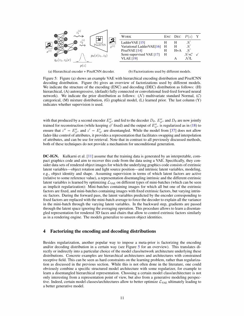
(a) Hierarchical encoder + PixelCNN decoder.

WORK ENC DEC P (z) Y

LadderVAE [15] H H NVariational LadderVAE[16] H H NPixelVAE [14] H H+A NSemi-supervised VAE [17] H N+C XVLAE [19] A N /L

(b) Factorizations used by different models.

Figure 5: Figure (a) shows an example VAE with hierarchical encoding distribution and PixelCNNdecoding distribution. Figure (b) gives an overview of factorizations used by different models.We indicate the structure of the encoding (ENC) and decoding (DEC) distribution as follows: (H)hierarchical, (A) autoregressive, (default) fully connected or convolutional feed-feed forward neuralnetwork). We indicate the prior distribution as follows: (N ) multivariate standard Normal, (C)categorical, (M) mixture distribution, (G) graphical model, (L) learned prior. The last column (Y)indicates whether supervision is used.

with that produced by a second encoderE′′φ′′ and fed to the decoderDθ. E′′φ′′ andDθ are now jointlytrained for reconstruction (while keeping φ′ fixed) and the output of E′′φ′′ is regularized as in (18) toensure that z′′ = E′′φ′′ and z′ = E′φ′ are disentangled. While the model from [37] does not allowfader-like control of attributes, it provides a representation that facilitates swapping and interpolationof attributes, and can be use for retrieval. Note that in contrast to all previously discussed methods,both of these techniques do not provide a mechanism for unconditional generation.

DC-IGN. Kulkarni et al. [11] assume that the training data is generated by an interpretable, com-pact graphics code and aim to recover this code from the data using a VAE. Specifically, they con-sider data sets of rendered object images for which the underlying graphics code consists of extrinsiclatent variables—object rotation and light source position—and intrinsic latent variables, modeling,e.g., object identity and shape. Assuming supervision in terms of which latent factors are active(relative to some reference value), a representation disentangling intrinsic and the different extrinsiclatent variables is learned by optimizing LVAE on different types of mini-batches (which can be seenas implicit regularization): Mini-batches containing images for which all but one of the extrinsicfactors are fixed, and mini-batches containing images with fixed extrinsic factors, but varying intrin-sic factors. During the forward pass, the latent variables predicted by the encoder corresponding tofixed factors are replaced with the mini-batch average to force the decoder to explain all the variancein the mini-batch through the varying latent variables. In the backward step, gradients are passedthrough the latent space ignoring the averaging operation. This procedure allows to learn a disentan-gled representation for rendered 3D faces and chairs that allow to control extrinsic factors similarlyas in a rendering engine. The models generalize to unseen object identities.

4 Factorizing the encoding and decoding distributions

Besides regularization, another popular way to impose a meta-prior is factorizing the encodingand/or decoding distribution in a certain way (see Figure 5 for an overview). This translates di-rectly or indirectly into a particular choice of the model class/network architecture underlying thesedistributions. Concrete examples are hierarchical architectures and architectures with constrainedreceptive field. This can be seen as hard constraints on the learning problem, rather than regulariza-tion as discussed in the previous section. While this is not often done in the literature, one couldobviously combine a specific structured model architecture with some regularizer, for example tolearn a disentangled hierarchical representation. Choosing a certain model class/architecture is notonly interesting from a representation point of view, but also from a generative modeling perspec-tive. Indeed, certain model classes/architectures allow to better optimize LVAE ultimately leading toa better generative model.

11

Semi-supervised VAE. Kingma et al. [17] harness the VAE framework for semi-supervised learn-ing. Specifically, in the “M2 model”, the latent code is divided into two parts z and y where y is(typically discrete) label information observed for a subset of the training data. More specifically,the inference model takes the form qφ(z, y|x) = qφ(z|y, x)qφ(y|x), i.e., there is a hierarchy betweeny and z. During training, for samples x(i) for which a label y(i) is a available, the inference model isconditioned on y (i.e., qφ(z|y, x)) and LVAE is adapted accordingly, and for samples without label,the label is inferred from qφ(z, y|x). This model hence effectively disentangles the latent code intotwo parts y and z and allows for semi-supervised classification and controlled generation by holdingone of the factors fixed and generating the other one. This model can optionally be combined with anadditional model learned in unsupervised fashion to obtain an additional level of hierarchy (termed“M1 + M2 model” in [17]).

VLAE. Analyzing the VAE framework through the lens of Bits-Back coding [52, 53], Chen et al.[19] identify the so-called information preference property: The second term in LVAE (1) encour-ages the latent code z ∼ qφ(z|x) to only store the information that cannot be modeled locally(i.e., unconditionally without using the latent code) by the decoding distribution pθ(x|z). As a con-sequence, when the decoding distribution is a powerful autoregressive model such as conditionalPixelRNN [54] or PixelCNN [49] the latent code will not be used to encode any information andqφ(z|x) will perfectly match the prior p(z), as previously observed by many authors. While this notnecessarily an issue in the context of generative modeling (where the goal is to maximize testinglog-likelihood), it is problematic from a representation learning point of view as one wants the latentcode z ∼ qφ(z|x) to store meaningful information. To overcome this issue, Chen et al. [19] proposeto adapt the structure of the decoding distribution pθ(x|z) such that it cannot model the informationone would like z to store, and term the resulting model variational lossy autoencoder (VLAE). Forexample, to encourage z to capture global high-level information, while letting pθ(x|z) model localinformation such as texture, one can use an autoregressive decoding distribution with a limited localreceptive field pθ(x|z) =

∏j pθ(xj |z, xW (j)), where W (j) is a window centered in pixel j, that

cannot model long-range spatial dependencies. Besides the implications of the information prefer-ence property for representation learning, Chen et al. [19] also explore the orthogonal direction ofusing a learned prior based on autoregressive flow [55] to improve generative modeling capabilitiesof VLAE.

PixelVAE. PixelVAEs [14] use a VAE with feed-forward convolutional encoder and de-coder, combining the decoder with a (shallow) conditional PixelCNN [49] to predict the out-put probabilities. Furthermore, they employ a hierarchical encoder and decoder structurewith multiple levels of latent variables. In more detail, the encoding and decoding distri-butions are factorized as qφ(z1, . . . , zL|x) = qφ(z1|x) . . . qφ(zL|x) and pθ(x, z1, . . . , zL) =pθ(x|z1)pθ(z1|z2) . . . pθ(zL−1|zL)p(zL). Here, z1, . . . , zL are groups of latent variables (ratherthan individual entries of z), the qφ(zj |x) are parametric distributions (typically Gaussian withdiagonal covariance matrix) whose parameters are predicted from different layers of the sameCNN (with layer index increasing in j), pθ(x|z1) is a conditional PixelCNN, and the factors inpθ(z1|z2) . . . pθ(zL−1|zL) are realized by a feed-forward convolutional networks. From a represen-tation learning perspective, this approach leads to the extraction of high- and low-level features onone hand, allowing for controlled generation of local and global structure, and on the other handresults in better clustering of the codes according to classes in the case of multi-class data. From agenerative modeling perspective, this approach obtains testing likelihood competitive with or betterthan computationally more complex (purely autoregressive) PixelCNN and PixelRNN models. OnlyL = 2 stochastic layers are explored experimentally.

LadderVAE. In contrast to PixelVAEs, Ladder VAEs (LVAEs) [15] perform top-down inference,i.e., the encoding distribution is factorized as qφ(z|x) = qφ(zL|x)

∏L−1j=1 qφ(zj |zj+1), while using

the same factorization for pθ(x|z) as PixelVAE (although employing a simple factorized Gaussiandistribution for pθ(x|z1) instead of a PixelCNN). The qφ(zj |zj+1) are parametrized Gaussian dis-tributions whose parameters are inferred top-down using a precision-weighted combination of (i)bottom-up predictions from different layers of the same feed-forward encoder CNN (similarly asin PixelVAE) with (ii) top-down predictions obtained by sampling from the hierarchical distributionpθ(z) = pθ(z1|z2) . . . pθ(zL−1|zL)p(zL) (see [15, Figure 1b] for the corresponding graphical modelrepresentation). When trained with a suitable warm-up procedure, LVAEs are capable of effectively

12

x(i) x(i)

z(i)µ

�

q�(z|x) p✓(x|z)

p(z)

encoder decoder

prior

x(i) x(i)

z(i)µ

�

q�(z|x) p✓(x|z)

p1(z) p2(z)

x(i)

x(i)

p(z)

z(i)1 z(i)2

µ1

µ2

�2

�1

q�(z1, z2|x)

p✓(x|z1, z2)

PixelCNN

or

code

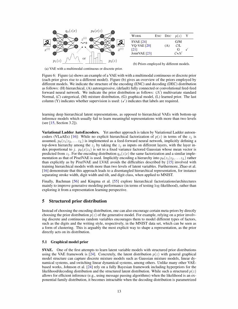
(a) VAE with a multimodal continuous or discrete prior.

WORK ENC DEC p(z) Y

SVAE [24] G/MVQ-VAE [20] (A) C/L[21] G XJointVAE [23] C+N

(b) Priors employed by different models.

Figure 6: Figure (a) shows an example of a VAE with with a multimodal continuous or discrete prior(each prior gives rise to a different model). Figure (b) gives an overview of the priors employed bydifferent models. We indicate the structure of the encoding (ENC) and decoding (DEC) distributionas follows: (H) hierarchical, (A) autoregressive, (default) fully connected or convolutional feed-feedforward neural network. We indicate the prior distribution as follows: (N ) multivariate standardNormal, (C) categorical, (M) mixture distribution, (G) graphical model, (L) learned prior. The lastcolumn (Y) indicates whether supervision is used: (X) indicates that labels are required.

learning deep hierarchical latent representations, as opposed to hierarchical VAEs with bottom-upinference models which usually fail to learn meaningful representations with more than two levels(see [15, Section 3.2]).

Variational Ladder AutoEncoders. Yet another approach is taken by Variational Ladder autoen-coders (VLaAEs) [16]: While no explicit hierarchical factorization of p(z) in terms of the zj isassumed, pθ(z1|z2, . . . zL) is implemented as a feed-forward neural network, implicitly defining atop-down hierarchy among the zj by taking the zj as inputs on different layers, with the layer in-dex proportional to j. pθ(x|z1) is set to a fixed variance factored Gaussian whose mean vector ispredicted from z1. For the encoding distribution qφ(z|x) the same factorization and a similar imple-mentation as that of PixelVAE is used. Implicitly encoding a hierarchy into pθ(z1|z2, . . . zL) ratherthan explicitly as by PixelVAE and LVAE avoids the difficulties described by [15] involved withtraining hierarchical models with more than two levels of latent variables. Furthermore, Zhao et al.[16] demonstrate that this approach leads to a disentangled hierarchical representation, for instanceseparating stroke width, digit width and tilt, and digit class, when applied to MNIST.

Finally, Bachman [56] and Kingma et al. [55] explore hierarchical factorizations/architecturesmainly to improve generative modeling performance (in terms of testing log-likelihood), rather thanexploring it from a representation learning perspective.

5 Structured prior distribution

Instead of choosing the encoding distribution, one can also encourage certain meta-priors by directlychoosing the prior distribution p(z) of the generative model. For example, relying on a prior involv-ing discrete and continuous random variables encourages them to model different types of factors,such as the digits and the writing style, respectively, in the MNIST data set, which can be seen asa form of clustering. This is arguably the most explicit way to shape a representation, as the priordirectly acts on its distribution.

5.1 Graphical model prior

SVAE. One of the first attempts to learn latent variable models with structured prior distributionsusing the VAE framework is [24]. Concretely, the latent distribution p(z) with general graphicalmodel structure can capture discrete mixture models such as Gaussian mixture models, linear dy-namical systems, and switching linear dynamical systems, among others. Unlike many other VAE-based works, Johnson et al. [24] rely on a fully Bayesian framework including hyperpriors for thelikelihood/decoding distribution and the structured latent distribution. While such a structured p(z)allows for efficient inference (e.g., using message passing algorithms) when the likelihood is an ex-ponential family distribution, it becomes intractable when the decoding distribution is parametrized

13

through a neural network as commonly done in the VAE framework, the reason for which the latterincludes an approximate posterior/encoding distribution. To combine the tractability of conjugategraphical model inference with the flexibility of VAEs, Johnson et al. [24] employ inference modelsthat output conjugate graphical model potentials [57] instead of the parameters of the approximateposterior distribution. In particular, these potentials are chosen such that they have a form conjugateto the exponential family, hence allowing for efficient inference when combined with the structuredp(z). The resulting algorithm is termed structured VAE (SVAE). Experiments show that SVAE witha Gaussian mixture prior learns a generative model whose latent mixture components reflect clustersin the data, and SVAE with a switching linear dynamical system prior learns a representation thatreflects behavior state transitions in motion recordings of mouses.

Narayanaswamy et al. [21] consider latent distributions with graphical model structure similar to[24], but they also incorporate partial supervision for some of the latent variables as [17]. However,unlike Kingma et al. [17] which assumes a posterior of the form qφ(z, y|x) = qφ(z|y, x)qφ(y|x),they do not assume a specific factorization of the partially observed latent variables y and the unob-served ones z (neither for qφ(z, y|x) nor for the marginals qφ(z|x) and qφ(y|x)), and no particulardistributional form of qφ(z|x) and qφ(y|x). To perform inference for qφ(z, y|x) with arbitrary de-pendence structure, Narayanaswamy et al. [21] derive a new Monte Carlo estimator. The proposedapproach is able to disentangle digit index and writing style on MNIST with partial supervision ofthe digit index (similar to [17]). Furthermore, this approach can disentangle identity and lightingdirection of face images with partial supervision assuming the product of categorical and continuousdistribution, respectively, for the prior (using the the Gumbel-Softmax estimator [58, 59] to modelthe categorical part in the approximate posterior).

5.2 Discrete latent variables

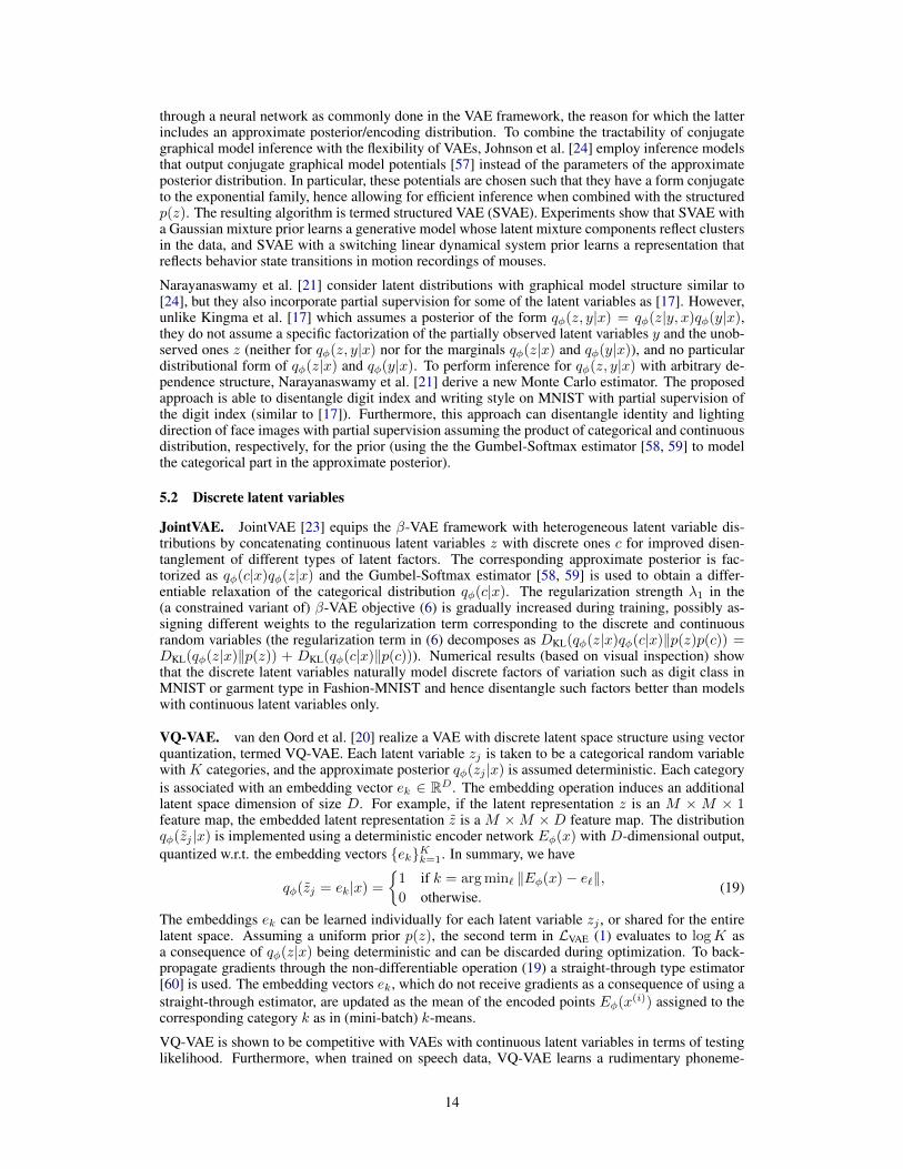
JointVAE. JointVAE [23] equips the β-VAE framework with heterogeneous latent variable dis-tributions by concatenating continuous latent variables z with discrete ones c for improved disen-tanglement of different types of latent factors. The corresponding approximate posterior is fac-torized as qφ(c|x)qφ(z|x) and the Gumbel-Softmax estimator [58, 59] is used to obtain a differ-entiable relaxation of the categorical distribution qφ(c|x). The regularization strength λ1 in the(a constrained variant of) β-VAE objective (6) is gradually increased during training, possibly as-signing different weights to the regularization term corresponding to the discrete and continuousrandom variables (the regularization term in (6) decomposes as DKL(qφ(z|x)qφ(c|x)‖p(z)p(c)) =DKL(qφ(z|x)‖p(z)) + DKL(qφ(c|x)‖p(c))). Numerical results (based on visual inspection) showthat the discrete latent variables naturally model discrete factors of variation such as digit class inMNIST or garment type in Fashion-MNIST and hence disentangle such factors better than modelswith continuous latent variables only.

VQ-VAE. van den Oord et al. [20] realize a VAE with discrete latent space structure using vectorquantization, termed VQ-VAE. Each latent variable zj is taken to be a categorical random variablewith K categories, and the approximate posterior qφ(zj |x) is assumed deterministic. Each categoryis associated with an embedding vector ek ∈ RD. The embedding operation induces an additionallatent space dimension of size D. For example, if the latent representation z is an M × M × 1feature map, the embedded latent representation z is a M ×M ×D feature map. The distributionqφ(zj |x) is implemented using a deterministic encoder network Eφ(x) with D-dimensional output,quantized w.r.t. the embedding vectors {ek}Kk=1. In summary, we have

qφ(zj = ek|x) ={1 if k = argmin` ‖Eφ(x)− e`‖,0 otherwise.

(19)

The embeddings ek can be learned individually for each latent variable zj , or shared for the entirelatent space. Assuming a uniform prior p(z), the second term in LVAE (1) evaluates to logK asa consequence of qφ(z|x) being deterministic and can be discarded during optimization. To back-propagate gradients through the non-differentiable operation (19) a straight-through type estimator[60] is used. The embedding vectors ek, which do not receive gradients as a consequence of using astraight-through estimator, are updated as the mean of the encoded points Eφ(x(i)) assigned to thecorresponding category k as in (mini-batch) k-means.

VQ-VAE is shown to be competitive with VAEs with continuous latent variables in terms of testinglikelihood. Furthermore, when trained on speech data, VQ-VAE learns a rudimentary phoneme-

14

level language model in a completely unsupervised fashion, which can be used for controlled speechgeneration and phoneme classification.

Many other works explore learning (variational) autoencoders with (vector-)quantized latent repre-sentation with a focus on generative modeling [61, 62, 58, 59] and compression [63], rather thanrepresentation learning.

6 Other approaches

Early approaches. Early approaches to learn abstract representations using autoencoders includestacking single-layer autoencoders [64] to build deep architectures and imposing a sparsity priorto the latent variables [65]. Another way to achieve abstraction is to require the representation tobe robust to noise. Such a representation can be learned using denoising autoencoders [66], i.e.,autoencoders trained to reconstruct clean data points from a noisy version. For a broader overviewover early approaches we refer to [1, Section 7].

Sequential data. There is a considerable number of recent works leveraging (variational) autoen-coders and the techniques similar to those outlined in Sections 3–5 to learn representations of se-quences. Yingzhen and Mandt [67] partition the latent code of a VAE into subsets of time varyingand time invariant variables (resulting in a particular factorization of the approximate posterior) tolearn a representation disentangling content and pose/identity in video/audio sequences. Hsieh et al.[68] use a similar partition of the latent code, but additionally allow the model to decompose theinput into different parts, e.g., modelling different moving objects in a video sequence. Somewhatrelated, Villegas et al. [69], Denton and Birodkar [70], Fraccaro et al. [71] propose autoencodermodels for video sequence prediction with separate encoders disentangling the latent code into poseand content. Hsu et al. [72] develop a hierarchical VAE model to learn interpretable representa-tions of speech recordings. Fortuin et al. [73] combine a variation of VQ-VAE with self-organizingmaps to learn interpretable discrete representations of sequences. Further, VAEs for sequences arealso of great interest in the context of natural language processing, in particular with autoregressiveencoders/decoders and discrete latent representations, see, e.g., [74–76] and references therein.

Using a discriminator in pixel space. An alternative to training a pair of probabilistic encoderqφ(z|x) and decoder pθ(x|z) to minimize a reconstruction loss is to learn φ, θ by matching thejoint distributions pθ(x|z)p(z) and qφ(z|x)p(x). To achieve this, adversarially learned inference(ALI) [77] and bidirectional GAN (BiGAN) [78] leverage the GAN framework, learning pθ(x|z),qφ(z|x) jointly with a discriminator to distinguish between samples drawn from the two joint distri-butions. While this approach yields powerful generative models with latent representations usefulfor downstream tasks, the reconstructions are less faithful than for autoencoder-based models. Liet al. [79] point out a non-identifiability issue inherent with the distribution matching problem un-derlying ALI/BiGAN, and propose to penalize the entropy of the reconstruction conditionally on thecode.

Chen et al. [80] augment a standard GAN framework [34] with a mutual information term betweenthe generator output and a subset of latent variables, which proves effective in learning disentan-gled representations. Other works regularize the output of (variational) autoencoders with a GANloss. Specifically, Larsen et al. [81], Rosca et al. [82] combine VAE with standard GAN [34], andTschannen et al. [83] equip AAE/WAE with a Wasserstein GAN loss [84]. While Larsen et al. [81]investigate the representation learned by their model, the focus of these works is on improving thesample quality of VAE and AAE/WAE. Mathieu et al. [85] rely on a similar setup as [81], but uselabels to learn disentangled representations.

Cross-domain disentanglement. Image-to-image translation methods [86, 87] (translating, e.g.,semantic label maps into images) can be implemented by training encoder-decoder architectures totranslate between two domains (i.e., in both directions) while enforcing the translated data to matchthe respective domain distribution. While this task as such does not a priori encourage learningof meaningful representation, adding appropriate pressure does: Sharing parts of the latent repre-sentation between the translation networks [27–29] and/or combining domain specific and sharedtranslation networks [88] leads to disentangled representations.

15

7 Rate-distortion tradeoff and usefulness of representation

In this paper we provided an overview of existing work on autoencoder-based representation learningapproaches. One common pattern is that methods targeting rather abstract meta-priors such as dis-entanglement (e.g., β-VAE [2]) were only applied to synthetic data sets and very structured real datasets at low resolution. In contrast, fully supervised methods, such as FaderNetworks [12], providerepresentations which capture subtle properties of the data, can be scaled to high-resolution data,and allow fine-grained control of the reconstructions by manipulating the representation. As such,there is a rather large disconnect between methods which have some knowledge of the downstreamtask and the methods which invent a proxy task based on a meta-prior. In this section, we considerthis aspect through the lens of rate-distortion tradeoffs based on appropriately defined notions of rateand distortion. Figure 7 illustrates our arguments.

Rate-distortion tradeoff for unsupervised learning. It can be shown that models based purely onoptimizing the marginal likelihood might be completely useless for representation learning. We willclosely follow the elegant exposition from Alemi et al. [30]. Consider the quantities

H = −∫p(x) log p(x) dx = Ep(x)[− log p(x)]

D = −∫∫

p(x)qφ(z|x) log pθ(x|z) dx dz = Ep(x)[Eqφ(z|x)[− log pθ(x|z)]]

R =

∫∫p(x)qφ(z|x) log

qφ(z|x)p(z)

dx dz = Ep(x)[DKL(qθ(z|x)‖p(z))]

where H corresponds to the entropy of the underlying data source, D the distortion (i.e., the re-construction negative log-likelihood), and R the rate, namely the average relative KL divergencebetween the encoding distribution and the p(z). Note that the ELBO objective is now simplyELBO = −LVAE = −(D + R) (or −(D + βR) for β-VAE). Alemi et al. [30] show that thefollowing inequality holds:

H −D ≤ R.

Figure 7 shows the resulting rate-distortion curve from Alemi et al. [30] in the limit of arbitrarypowerful encoders and decoders. The horizontal line (R, 0) corresponds to the setting where oneis able to encode and decode the data with no distortion at a rate of H . The vertical line (0, D)corresponds to the zero-rate setting and by choosing a sufficiently powerful decoder one can reachthe distortion of H . A critical issue is that any point on the line D = H − R achieves the sameELBO. As a result, models based purely on optimizing the marginal likelihood might be completelyuseless for representation learning [30, 89] as there is no incentive to choose a point with a highrate (corresponding to an informative code). This effect is prominent in many models employingpowerful decoders which function close to the zero-rate regime (see Section 4 for details). As asolution, Alemi et al. [30] suggest to optimize the same model under a constraint on the desired rateσ, namely to solve minφ,θD + |σ − R|. However, is this really enough to learn representationsuseful for a specific downstream task?

The rate-distortion-usefulness tradeoff. Here we argue that even if one is able to reach any desiredrate-distortion tradeoff point, in particular targeting a representation with specific rateR, the learnedrepresentation might still be useless for a specific downstream task. This stems from the fact that

(i) it is unclear which part of the total information (entropy) is stored in z and which part isstored in the decoder, and

(ii) even if the information relevant for the downstream task is stored in z, there is no guaranteethat it is stored in a form that can be exploited by the model used to solve the downstreamtask.

For example, regarding (i), if the downstream task is an image classification task, the representationshould store the object class or the most prominent object features. On the other hand, if the down-stream task is to recognize relative ordering of objects, the locations have to be encoded instead.Concerning (ii), if we use a linear model on top of the representation as often done in practice, therepresentation needs to have structure amenable to linear prediction.

16

(a) Rate-distortion (R-D) tradeoff of [30].

feasible

infeasible

realizable

R0

Dy

I(x; y)

H(y|x)

H(y)

(b) R-Dy tradeoff for the supervised case.

R D

M1

R1

D1

D2

R2

M2

“usefulness”

0

(c) Rate-distortion-usefulness tradeoff.

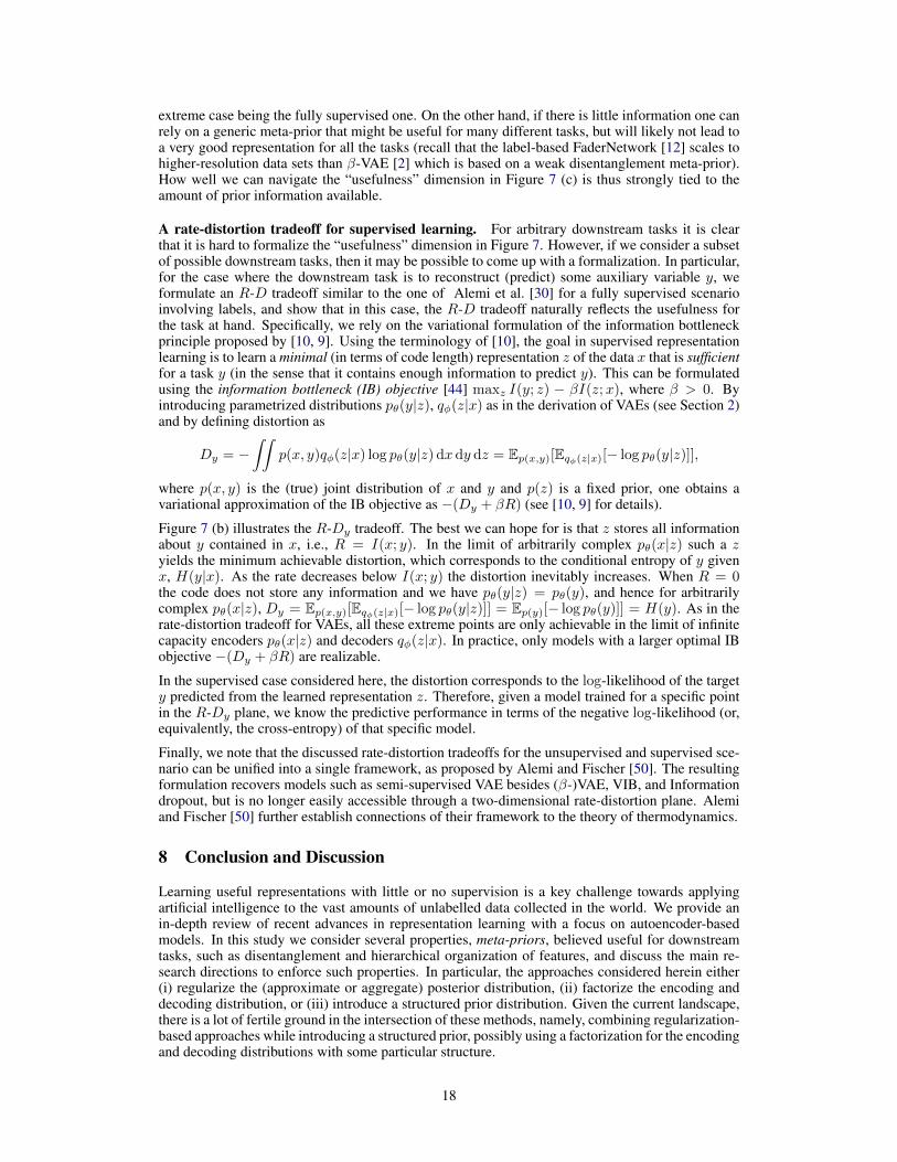
Figure 7: Figure (a) shows the Rate-distortion (R-D) tradeoff from [30], where D corresponds tothe reconstruction term in the (β-)VAE objective, and the rate to the KL term. Figure (b) shows asimilar tradeoff for the supervised case considered in [10, 9]. The ELBO −LVAE = −(R+D) doesnot reflect the usefulness of the learned representation for an unknown downstream task (see text),as illustrated in Figure (c).

We argue that there is no natural way to incorporate this desiderata directly into the classic R-D tradeoff embodied by the ELBO. Indeed, the R-D tradeoff per se does not account for whatinformation is stored in the representation and in what form, but only for how much.

Therefore, we suggest a third dimension, namely “usefulness” of the representation, which is or-thogonal to the R-D plane as shown in Figure 7. Consider two models M1 and M2 whose ratessatisfy R1 > R2 and D1 < D2 and which we want to use for the (a priori unknown) downstreamtask y (say image classification). It can be seen that M2 is more useful (as measured, for example,in terms of classification accuracy) for y even though it has a smaller rate and and a larger distortionthan M2. This can occur, for example, if the representation of M1 stores the object locations, butmodels the objects themselves with the decoder, whereas M1 produces blurry reconstructions, butlearns a representation that is more informative about object classes.

As discussed in Sections 3, 4, and 5, regularizers and architecture design choices can be used todetermine what information is captured by the representation and the decoder, and how it is mod-eled. Therefore, the regularizers and architecture not only allow us to navigate the R-D plane butsimultaneously also the “usefulness” dimension of our representation. As usefulness is always tiedto (i) a task (in the previous example, if we consider localization instead of classification, M1 wouldbe more useful than M2) and (ii) a model to solve the downstream task, this implies that one cannotguarantee usefulness of a representation for a task unless it is known in advance. Further, the betterthe task is known the easier it is to come up with suitable regularizers and network architectures, the

17

extreme case being the fully supervised one. On the other hand, if there is little information one canrely on a generic meta-prior that might be useful for many different tasks, but will likely not lead toa very good representation for all the tasks (recall that the label-based FaderNetwork [12] scales tohigher-resolution data sets than β-VAE [2] which is based on a weak disentanglement meta-prior).How well we can navigate the “usefulness” dimension in Figure 7 (c) is thus strongly tied to theamount of prior information available.

A rate-distortion tradeoff for supervised learning. For arbitrary downstream tasks it is clearthat it is hard to formalize the “usefulness” dimension in Figure 7. However, if we consider a subsetof possible downstream tasks, then it may be possible to come up with a formalization. In particular,for the case where the downstream task is to reconstruct (predict) some auxiliary variable y, weformulate an R-D tradeoff similar to the one of Alemi et al. [30] for a fully supervised scenarioinvolving labels, and show that in this case, the R-D tradeoff naturally reflects the usefulness forthe task at hand. Specifically, we rely on the variational formulation of the information bottleneckprinciple proposed by [10, 9]. Using the terminology of [10], the goal in supervised representationlearning is to learn a minimal (in terms of code length) representation z of the data x that is sufficientfor a task y (in the sense that it contains enough information to predict y). This can be formulatedusing the information bottleneck (IB) objective [44] maxz I(y; z) − βI(z;x), where β > 0. Byintroducing parametrized distributions pθ(y|z), qφ(z|x) as in the derivation of VAEs (see Section 2)and by defining distortion as

Dy = −∫∫

p(x, y)qφ(z|x) log pθ(y|z) dxdy dz = Ep(x,y)[Eqφ(z|x)[− log pθ(y|z)]],

where p(x, y) is the (true) joint distribution of x and y and p(z) is a fixed prior, one obtains avariational approximation of the IB objective as −(Dy + βR) (see [10, 9] for details).

Figure 7 (b) illustrates the R-Dy tradeoff. The best we can hope for is that z stores all informationabout y contained in x, i.e., R = I(x; y). In the limit of arbitrarily complex pθ(x|z) such a zyields the minimum achievable distortion, which corresponds to the conditional entropy of y givenx, H(y|x). As the rate decreases below I(x; y) the distortion inevitably increases. When R = 0the code does not store any information and we have pθ(y|z) = pθ(y), and hence for arbitrarilycomplex pθ(x|z), Dy = Ep(x,y)[Eqφ(z|x)[− log pθ(y|z)]] = Ep(y)[− log pθ(y)]] = H(y). As in therate-distortion tradeoff for VAEs, all these extreme points are only achievable in the limit of infinitecapacity encoders pθ(x|z) and decoders qφ(z|x). In practice, only models with a larger optimal IBobjective −(Dy + βR) are realizable.

In the supervised case considered here, the distortion corresponds to the log-likelihood of the targety predicted from the learned representation z. Therefore, given a model trained for a specific pointin the R-Dy plane, we know the predictive performance in terms of the negative log-likelihood (or,equivalently, the cross-entropy) of that specific model.

Finally, we note that the discussed rate-distortion tradeoffs for the unsupervised and supervised sce-nario can be unified into a single framework, as proposed by Alemi and Fischer [50]. The resultingformulation recovers models such as semi-supervised VAE besides (β-)VAE, VIB, and Informationdropout, but is no longer easily accessible through a two-dimensional rate-distortion plane. Alemiand Fischer [50] further establish connections of their framework to the theory of thermodynamics.

8 Conclusion and Discussion

Learning useful representations with little or no supervision is a key challenge towards applyingartificial intelligence to the vast amounts of unlabelled data collected in the world. We provide anin-depth review of recent advances in representation learning with a focus on autoencoder-basedmodels. In this study we consider several properties, meta-priors, believed useful for downstreamtasks, such as disentanglement and hierarchical organization of features, and discuss the main re-search directions to enforce such properties. In particular, the approaches considered herein either(i) regularize the (approximate or aggregate) posterior distribution, (ii) factorize the encoding anddecoding distribution, or (iii) introduce a structured prior distribution. Given the current landscape,there is a lot of fertile ground in the intersection of these methods, namely, combining regularization-based approaches while introducing a structured prior, possibly using a factorization for the encodingand decoding distributions with some particular structure.

18

Unsupervised representation learning is an ill-defined problem if the downstream task can be arbi-trary. Hence, all current methods use strong inductive biases and modeling assumptions. Implicitor explicit supervision remains a key enabler and, depending on the mechanism for enforcing meta-priors, different degrees of supervision are required. One can observe a clear tradeoff between thedegree of supervision and how useful the resulting representation is: On one end of the spectrum aremethods targeting abstract meta-priors such as disentanglement (e.g., β-VAE [2]) that were appliedmainly to toy-like data sets. On the other end of the spectrum are fully supervised methods (e.g.,FaderNetworks [12]) where the learned representations capture subtle aspects of the data, allow forfine-grained control of the reconstructions by manipulating the representation, and are amenable tohigher-dimensional data sets. Furthermore, through the lens of rate-distortion we argue that, perhapsunsurprisingly, maximum likelihood optimization alone can’t guarantee that the learned represen-tation is useful at all. One way to sidestep this fundamental issue is to consider the ”usefulness”dimension with respect to a given task (or a distribution of tasks) explicitly.

19

References[1] Y. Bengio, A. Courville, and P. Vincent, “Representation learning: A review and new perspec-

tives,” IEEE Transactions on Pattern Analysis and Machine Intelligence, vol. 35, no. 8, pp.1798–1828, 2013.

[2] I. Higgins, L. Matthey, A. Pal, C. Burgess, X. Glorot, M. Botvinick, S. Mohamed, and A. Ler-chner, “beta-VAE: Learning basic visual concepts with a constrained variational framework,”in International Conference on Learning Representations, 2017.

[3] H. Kim and A. Mnih, “Disentangling by factorising,” in Proc. of the International Conferenceon Machine Learning, 2018, pp. 2649–2658.

[4] T. Q. Chen, X. Li, R. Grosse, and D. Duvenaud, “Isolating sources of disentanglement invariational autoencoders,” in Advances in Neural Information Processing Systems, 2018.

[5] S. Zhao, J. Song, and S. Ermon, “InfoVAE: Information maximizing variational autoencoders,”arXiv:1706.02262, 2017.

[6] A. Kumar, P. Sattigeri, and A. Balakrishnan, “Variational inference of disentangled latent con-cepts from unlabeled observations,” in International Conference on Learning Representations,2018.

[7] R. Lopez, J. Regier, M. I. Jordan, and N. Yosef, “Information constraints on auto-encodingvariational bayes,” in Advances in Neural Information Processing Systems, 2018.

[8] B. Esmaeili, H. Wu, S. Jain, A. Bozkurt, N. Siddharth, B. Paige, D. H. Brooks, J. Dy, and J.-W.van de Meent, “Structured disentangled representations,” arXiv:1804.02086, 2018.

[9] A. A. Alemi, I. Fischer, J. V. Dillon, and K. Murphy, “Deep variational information bottleneck,”in International Conference on Learning Representations, 2016.

[10] A. Achille and S. Soatto, “Information dropout: Learning optimal representations throughnoisy computation,” IEEE Transactions on Pattern Analysis and Machine Intelligence, 2018.

[11] T. D. Kulkarni, W. F. Whitney, P. Kohli, and J. Tenenbaum, “Deep convolutional inverse graph-ics network,” in Advances in Neural Information Processing Systems, 2015, pp. 2539–2547.

[12] G. Lample, N. Zeghidour, N. Usunier, A. Bordes, L. Denoyer et al., “Fader networks: Manip-ulating images by sliding attributes,” in Advances in Neural Information Processing Systems,2017, pp. 5967–5976.

[13] C. Louizos, K. Swersky, Y. Li, M. Welling, and R. Zemel, “The variational fair autoencoder,”in International Conference on Learning Representations, 2016.

[14] I. Gulrajani, K. Kumar, F. Ahmed, A. A. Taiga, F. Visin, D. Vazquez, and A. Courville, “Pix-elVAE: A latent variable model for natural images,” in International Conference on LearningRepresentations, 2017.

[15] C. K. Sønderby, T. Raiko, L. Maaløe, S. K. Sønderby, and O. Winther, “Ladder variationalautoencoders,” in Advances in Neural Information Processing Systems, 2016, pp. 3738–3746.

[16] S. Zhao, J. Song, and S. Ermon, “Learning hierarchical features from deep generative models,”in Proc. of the International Conference on Machine Learning, 2017, pp. 4091–4099.

[17] D. P. Kingma, S. Mohamed, D. J. Rezende, and M. Welling, “Semi-supervised learning withdeep generative models,” in Advances in Neural Information Processing Systems, 2014, pp.3581–3589.

[18] A. Makhzani and B. J. Frey, “PixelGAN autoencoders,” in Advances in Neural InformationProcessing Systems, 2017, pp. 1975–1985.

[19] X. Chen, D. P. Kingma, T. Salimans, Y. Duan, P. Dhariwal, J. Schulman, I. Sutskever, andP. Abbeel, “Variational lossy autoencoder,” in International Conference on Learning Repre-sentations, 2017.

20

[20] A. van den Oord, O. Vinyals et al., “Neural discrete representation learning,” in Advances inNeural Information Processing Systems, 2017, pp. 6306–6315.

[21] S. Narayanaswamy, T. B. Paige, J.-W. Van de Meent, A. Desmaison, N. Goodman, P. Kohli,F. Wood, and P. Torr, “Learning disentangled representations with semi-supervised deep gen-erative models,” in Advances in Neural Information Processing Systems, 2017, pp. 5925–5935.

[22] A. Makhzani, J. Shlens, N. Jaitly, I. Goodfellow, and B. Frey, “Adversarial autoencoders,”arXiv:1511.05644, 2015.

[23] E. Dupont, “Learning disentangled joint continuous and discrete representations,” in Advancesin Neural Information Processing Systems, 2018.

[24] M. Johnson, D. K. Duvenaud, A. Wiltschko, R. P. Adams, and S. R. Datta, “Composing graphi-cal models with neural networks for structured representations and fast inference,” in Advancesin Neural Information Processing Systems, 2016, pp. 2946–2954.

[25] D. P. Kingma and M. Welling, “Auto-encoding variational bayes,” in International Conferenceon Learning Representations, 2014.

[26] D. J. Rezende, S. Mohamed, and D. Wierstra, “Stochastic backpropagation and approximateinference in deep generative models,” in Proc. of the International Conference on MachineLearning, 2014, pp. 1278–1286.

[27] Y.-C. Liu, Y.-Y. Yeh, T.-C. Fu, S.-D. Wang, W.-C. Chiu, and Y.-C. F. Wang, “Detach and adapt:Learning cross-domain disentangled deep representation,” in Proc. of the IEEE Conference onComputer Vision and Pattern Recognition, 2017.

[28] H.-Y. Lee, H.-Y. Tseng, J.-B. Huang, M. Singh, and M.-H. Yang, “Diverse image-to-imagetranslation via disentangled representations,” in Proc. of the European Conference on Com-puter Vision, 2018, pp. 35–51.

[29] A. Gonzalez-Garcia, J. van de Weijer, and Y. Bengio, “Image-to-image translation for cross-domain disentanglement,” in Advances in Neural Information Processing Systems, 2018.

[30] A. Alemi, B. Poole, I. Fischer, J. Dillon, R. A. Saurous, and K. Murphy, “Fixing a brokenELBO,” in Proc. of the International Conference on Machine Learning, 2018, pp. 159–168.

[31] C. Doersch, “Tutorial on variational autoencoders,” arXiv:1606.05908, 2016.

[32] X. Nguyen, M. J. Wainwright, and M. I. Jordan, “Estimating divergence functionals and thelikelihood ratio by convex risk minimization,” IEEE Transactions on Information Theory,vol. 56, no. 11, pp. 5847–5861, 2010.

[33] M. Sugiyama, T. Suzuki, and T. Kanamori, “Density-ratio matching under the bregman diver-gence: a unified framework of density-ratio estimation,” Annals of the Institute of StatisticalMathematics, vol. 64, no. 5, pp. 1009–1044, 2012.

[34] I. Goodfellow, J. Pouget-Abadie, M. Mirza, B. Xu, D. Warde-Farley, S. Ozair, A. Courville,and Y. Bengio, “Generative adversarial nets,” in Advances in Neural Information ProcessingSystems, 2014, pp. 2672–2680.

[35] A. Gretton, K. M. Borgwardt, M. J. Rasch, B. Scholkopf, and A. Smola, “A kernel two-sampletest,” Journal of Machine Learning Research, vol. 13, no. Mar, 2012.

[36] I. Tolstikhin, O. Bousquet, S. Gelly, and B. Schoelkopf, “Wasserstein auto-encoders,” in Inter-national Conference on Learning Representations, 2018.

[37] N. Hadad, L. Wolf, and M. Shahar, “A two-step disentanglement method,” in Proc. of the IEEEConference on Computer Vision and Pattern Recognition, 2018, pp. 772–780.

[38] Z. Liu, P. Luo, X. Wang, and X. Tang, “Deep learning face attributes in the wild,” in Proc. ofthe IEEE International Conference on Computer Vision, 2015, pp. 3730–3738.

21

[39] P. Paysan, R. Knothe, B. Amberg, S. Romdhani, and T. Vetter, “A 3d face model for poseand illumination invariant face recognition,” in Proc. of the IEEE International Conference onAdvanced Video and Signal Based Surveillance. Ieee, 2009, pp. 296–301.

[40] M. Aubry, D. Maturana, A. A. Efros, B. C. Russell, and J. Sivic, “Seeing 3d chairs: exem-plar part-based 2d-3d alignment using a large dataset of cad models,” in Proc. of the IEEEConference on Computer Vision and Pattern Recognition, 2014, pp. 3762–3769.

[41] C. Eastwood and C. K. I. Williams, “A framework for the quantitative evaluation of disentan-gled representations,” in International Conference on Learning Representations, 2018.

[42] K. Ridgeway and M. C. Mozer, “Learning deep disentangled embeddings with the f-statisticloss,” in Advances in Neural Information Processing Systems, 2018.

[43] C. P. Burgess, I. Higgins, A. Pal, L. Matthey, N. Watters, G. Desjardins, and A. Lerchner,“Understanding disentangling in β-VAE,” arXiv:1804.03599, 2018.

[44] N. Tishby, F. C. Pereira, and W. Bialek, “The information bottleneck method,” arXiv preprintphysics/0004057, 2000.

[45] M. D. Hoffman and M. J. Johnson, “Elbo surgery: yet another way to carve up the variationalevidence lower bound,” in Workshop in Advances in Approximate Bayesian Inference, NIPS,2016.

[46] S. Watanabe, “Information theoretical analysis of multivariate correlation,” IBM Journal ofResearch and Development, vol. 4, no. 1, pp. 66–82, 1960.

[47] Q. Liu and D. Wang, “Stein variational gradient descent: A general purpose bayesian inferencealgorithm,” in Advances In Neural Information Processing Systems, 2016, pp. 2378–2386.

[48] A. Gretton, O. Bousquet, A. Smola, and B. Scholkopf, “Measuring statistical dependencewith Hilbert-Schmidt norms,” in International Conference on Algorithmic Learning Theory.Springer, 2005, pp. 63–77.

[49] A. van den Oord, N. Kalchbrenner, L. Espeholt, O. Vinyals, and A. Graves, “Conditional imagegeneration with PixelCNN decoders,” in Advances in Neural Information Processing Systems,2016, pp. 4790–4798.

[50] A. A. Alemi and I. Fischer, “TherML: Thermodynamics of machine learning,”arXiv:1807.04162, 2018.

[51] A. Rahimi and B. Recht, “Random features for large-scale kernel machines,” in Advances inNeural Information Processing Systems, 2008, pp. 1177–1184.

[52] G. E. Hinton and D. Van Camp, “Keeping the neural networks simple by minimizing the de-scription length of the weights,” in Proc. of the Annual Conference on Computational LearningTheory, 1993, pp. 5–13.

[53] A. Honkela and H. Valpola, “Variational learning and bits-back coding: An information-theoretic view to bayesian learning,” IEEE Transactions on Neural Networks, vol. 15, no. 4,pp. 800–810, 2004.

[54] A. Van Oord, N. Kalchbrenner, and K. Kavukcuoglu, “Pixel recurrent neural networks,” inInternational Conference on Machine Learning, 2016, pp. 1747–1756.

[55] D. P. Kingma, T. Salimans, R. Jozefowicz, X. Chen, I. Sutskever, and M. Welling, “Improvedvariational inference with inverse autoregressive flow,” in Advances in Neural InformationProcessing Systems, 2016, pp. 4743–4751.

[56] P. Bachman, “An architecture for deep, hierarchical generative models,” in Advances in NeuralInformation Processing Systems, 2016, pp. 4826–4834.

[57] M. J. Wainwright and M. I. Jordan, “Graphical models, exponential families, and variationalinference,” Foundations and Trends R© in Machine Learning, vol. 1, no. 1–2, pp. 1–305, 2008.

22

[58] E. Jang, S. Gu, and B. Poole, “Categorical reparameterization with Gumbel-softmax,” in Inter-national Conference on Learning Representations, 2017.

[59] C. J. Maddison, A. Mnih, and Y. W. Teh, “The concrete distribution: A continuous relaxationof discrete random variables,” in International Conference on Learning Representations, 2016.

[60] Y. Bengio, N. Leonard, and A. Courville, “Estimating or propagating gradients throughstochastic neurons for conditional computation,” arXiv:1308.3432, 2013.

[61] A. Mnih and K. Gregor, “Neural variational inference and learning in belief networks,” in Proc.of the International Conference on Machine Learning, 2014, pp. 1791–1799.

[62] A. Mnih and D. J. Rezende, “Variational inference for monte carlo objectives,” in Proc. of theInternational Conference on Machine Learning, 2016, pp. 2188–2196.

[63] E. Agustsson, F. Mentzer, M. Tschannen, L. Cavigelli, R. Timofte, L. Benini, and L. V. Gool,“Soft-to-hard vector quantization for end-to-end learning compressible representations,” in Ad-vances in Neural Information Processing Systems, 2017, pp. 1141–1151.

[64] Y. Bengio, P. Lamblin, D. Popovici, and H. Larochelle, “Greedy layer-wise training of deepnetworks,” in Advances In Neural Information Processing Systems, 2007, pp. 153–160.

[65] M. A. Ranzato, C. Poultney, S. Chopra, and Y. LeCun, “Efficient learning of sparse represen-tations with an energy-based model,” in Advances in Neural Information Processing Systems,2007, pp. 1137–1144.

[66] P. Vincent, H. Larochelle, Y. Bengio, and P.-A. Manzagol, “Extracting and composing robustfeatures with denoising autoencoders,” in Proc. of the International Conference on MachineLearning, 2008, pp. 1096–1103.

[67] L. Yingzhen and S. Mandt, “Disentangled sequential autoencoder,” in Proc. of the InternationalConference on Machine Learning, 2018, pp. 5656–5665.

[68] J.-T. Hsieh, B. Liu, D.-A. Huang, L. Fei-Fei, and J. C. Niebles, “Learning to decompose anddisentangle representations for video prediction,” in Advances in Neural Information Process-ing Systems, 2018.

[69] R. Villegas, J. Yang, S. Hong, X. Lin, and H. Lee, “Decomposing motion and content fornatural video sequence prediction,” in International Conference on Learning Representations,2017.

[70] E. L. Denton and V. Birodkar, “Unsupervised learning of disentangled representations fromvideo,” in Advances in Neural Information Processing Systems, 2017, pp. 4414–4423.

[71] M. Fraccaro, S. Kamronn, U. Paquet, and O. Winther, “A disentangled recognition and nonlin-ear dynamics model for unsupervised learning,” in Advances in Neural Information ProcessingSystems, 2017, pp. 3601–3610.

[72] W.-N. Hsu, Y. Zhang, and J. Glass, “Unsupervised learning of disentangled and interpretablerepresentations from sequential data,” in Advances in Neural Information Processing Systems,2017, pp. 1878–1889.

[73] V. Fortuin, M. Huser, F. Locatello, H. Strathmann, and G. Ratsch, “Deep self-organization:Interpretable discrete representation learning on time series,” arXiv:1806.02199, 2018.

[74] S. R. Bowman, L. Vilnis, O. Vinyals, A. Dai, R. Jozefowicz, and S. Bengio, “Generatingsentences from a continuous space,” in Proc. of the SIGNLL Conference on ComputationalNatural Language Learning, 2016, pp. 10–21.

[75] Z. Hu, Z. Yang, X. Liang, R. Salakhutdinov, and E. P. Xing, “Toward controlled generation oftext,” in Proc. of the International Conference on Machine Learning, 2017, pp. 1587–1596.

[76] I. V. Serban, A. Sordoni, R. Lowe, L. Charlin, J. Pineau, A. C. Courville, and Y. Bengio, “Ahierarchical latent variable encoder-decoder model for generating dialogues.” in AAAI, 2017,pp. 3295–3301.

23

[77] V. Dumoulin, I. Belghazi, B. Poole, O. Mastropietro, A. Lamb, M. Arjovsky, and A. Courville,“Adversarially learned inference,” in International Conference on Learning Representations,2017.

[78] J. Donahue, P. Krahenbuhl, and T. Darrell, “Adversarial feature learning,” in InternationalConference on Learning Representations, 2017.

[79] C. Li, H. Liu, C. Chen, Y. Pu, L. Chen, R. Henao, and L. Carin, “Alice: Towards understand-ing adversarial learning for joint distribution matching,” in Advances in Neural InformationProcessing Systems, 2017, pp. 5495–5503.

[80] X. Chen, Y. Duan, R. Houthooft, J. Schulman, I. Sutskever, and P. Abbeel, “InfoGAN: In-terpretable representation learning by information maximizing generative adversarial nets,” inAdvances in Neural Information Processing Systems, 2016, pp. 2172–2180.

[81] A. B. L. Larsen, S. K. Sønderby, H. Larochelle, and O. Winther, “Autoencoding beyond pixelsusing a learned similarity metric,” arXiv:1512.09300, 2015.

[82] M. Rosca, B. Lakshminarayanan, D. Warde-Farley, and S. Mohamed, “Variational approachesfor auto-encoding generative adversarial networks,” arXiv:1706.04987, 2017.

[83] M. Tschannen, E. Agustsson, and M. Lucic, “Deep generative models for distribution-preserving lossy compression,” in Advances in Neural Information Processing Systems, 2018.

[84] M. Arjovsky, S. Chintala, and L. Bottou, “Wasserstein generative adversarial networks,” inProc. of the International Conference on Machine Learning, vol. 70, 2017, pp. 214–223.

[85] M. F. Mathieu, J. J. Zhao, J. Zhao, A. Ramesh, P. Sprechmann, and Y. LeCun, “Disentanglingfactors of variation in deep representation using adversarial training,” in Advances in NeuralInformation Processing Systems 29, 2016, pp. 5040–5048.

[86] P. Isola, J.-Y. Zhu, T. Zhou, and A. A. Efros, “Image-to-image translation with conditional ad-versarial networks,” in Proc. of the IEEE Conference on Computer Vision and Pattern Recog-nition, 2017, pp. 5967–5976.

[87] J.-Y. Zhu, T. Park, P. Isola, and A. A. Efros, “Unpaired image-to-image translation using cycle-consistent adversarial networks,” in Proc. of the IEEE International Conference on ComputerVision, 2017, pp. 2242–2251.

[88] A. Liu, Y.-C. Liu, Y.-Y. Yeh, and Y.-C. F. Wang, “A unified feature disentangler for multi-domain image translation and manipulation,” in Advances in Neural Information ProcessingSystems, 2018.

[89] F. Huszar, “Is maximum likelihood useful for representation learning?” http://www.inference.vc/maximum-likelihood-for-representation-learning-2.

24

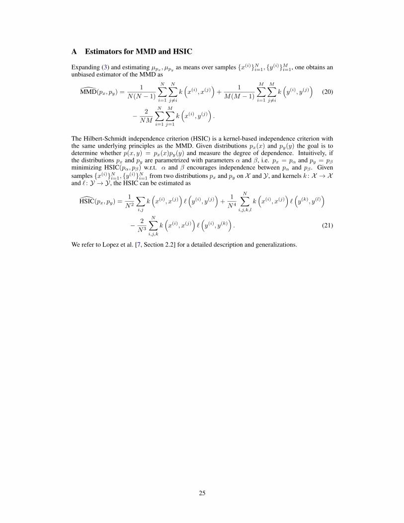
A Estimators for MMD and HSIC

Expanding (3) and estimating µpx , µpy as means over samples {x(i)}Ni=1, {y(i)}Mi=1, one obtains anunbiased estimator of the MMD as

MMD(px, py) =1

N(N − 1)

N∑i=1

N∑j 6=i

k(x(i), x(j)

)+

1

M(M − 1)

M∑i=1

M∑j 6=i

k(y(i), y(j)

)(20)

− 2

NM

N∑i=1

M∑j=1

k(x(i), y(j)

).

The Hilbert-Schmidt independence criterion (HSIC) is a kernel-based independence criterion withthe same underlying principles as the MMD. Given distributions px(x) and py(y) the goal is todetermine whether p(x, y) = px(x)py(y) and measure the degree of dependence. Intuitively, ifthe distributions px and py are parametrized with parameters α and β, i.e. px = pα and py = pβminimizing HSIC(pα, pβ) w.r.t. α and β encourages independence between pα and pβ . Givensamples {x(i)}Ni=1, {y(i)}Ni=1 from two distributions px and py on X and Y , and kernels k : X → Xand ` : Y → Y , the HSIC can be estimated as

HSIC(px, py) =1

N2

∑i,j

k(x(i), x(j)

)`(y(i), y(j)

)+

1

N4

N∑i,j,k,l

k(x(i), x(j)

)`(y(k), y(l)

)

− 2

N3

N∑i,j,k

k(x(i), x(j)

)`(y(i), y(k)

). (21)

We refer to Lopez et al. [7, Section 2.2] for a detailed description and generalizations.

25

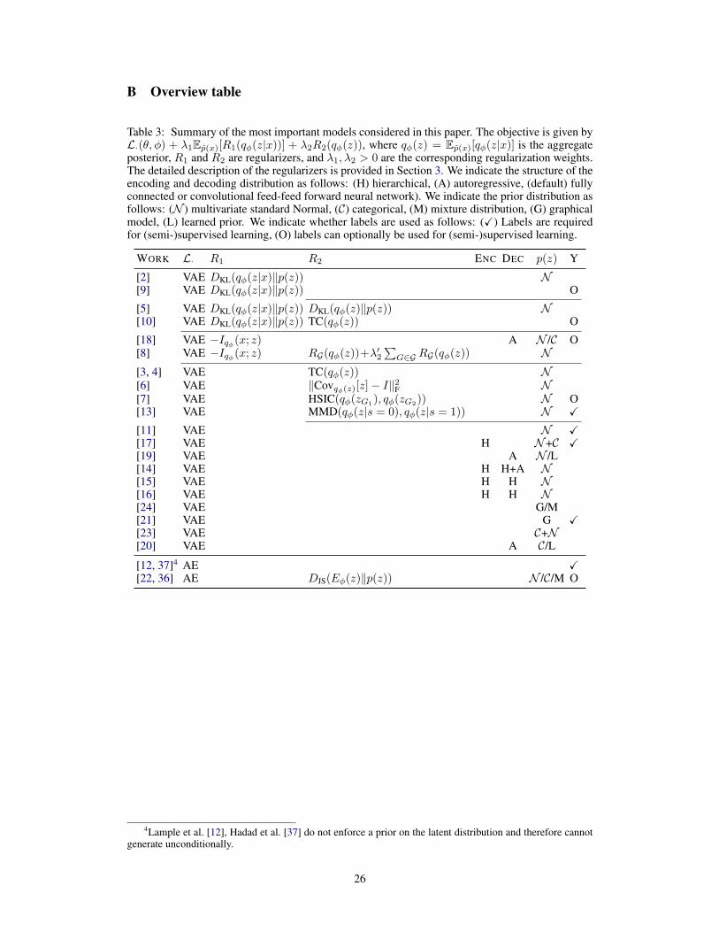
B Overview table

Table 3: Summary of the most important models considered in this paper. The objective is given byL·(θ, φ) + λ1Ep(x)[R1(qφ(z|x))] + λ2R2(qφ(z)), where qφ(z) = Ep(x)[qφ(z|x)] is the aggregateposterior, R1 and R2 are regularizers, and λ1, λ2 > 0 are the corresponding regularization weights.The detailed description of the regularizers is provided in Section 3. We indicate the structure of theencoding and decoding distribution as follows: (H) hierarchical, (A) autoregressive, (default) fullyconnected or convolutional feed-feed forward neural network). We indicate the prior distribution asfollows: (N ) multivariate standard Normal, (C) categorical, (M) mixture distribution, (G) graphicalmodel, (L) learned prior. We indicate whether labels are used as follows: (X) Labels are requiredfor (semi-)supervised learning, (O) labels can optionally be used for (semi-)supervised learning.

WORK L· R1 R2 ENC DEC p(z) Y

[2] VAE DKL(qφ(z|x)‖p(z)) N[9] VAE DKL(qφ(z|x)‖p(z)) O

[5] VAE DKL(qφ(z|x)‖p(z)) DKL(qφ(z)‖p(z)) N[10] VAE DKL(qφ(z|x)‖p(z)) TC(qφ(z)) O

[18] VAE −Iqφ(x; z) A N /C O[8] VAE −Iqφ(x; z) RG(qφ(z))+λ

′2

∑G∈G RG(qφ(z)) N

[3, 4] VAE TC(qφ(z)) N[6] VAE ‖Covqφ(z)[z]− I‖2F N[7] VAE HSIC(qφ(zG1

), qφ(zG2)) N O

[13] VAE MMD(qφ(z|s = 0), qφ(z|s = 1)) N X[11] VAE N X[17] VAE H N+C X[19] VAE A N /L[14] VAE H H+A N[15] VAE H H N[16] VAE H H N[24] VAE G/M[21] VAE G X[23] VAE C+N[20] VAE A C/L

[12, 37]4 AE X[22, 36] AE DJS(Eφ(z)‖p(z)) N /C/M O

4Lample et al. [12], Hadad et al. [37] do not enforce a prior on the latent distribution and therefore cannotgenerate unconditionally.

26