RECENT ADVANCES IN MATHEMATICAL MORPHOLOGY

Serge BEUCHERCentre de Morphologie Mathématique

Ecole des Mines de ParisFONTAINEBLEAU - France

Abstract=====================================

This paper aims at presenting some recent advances in mathematicalmorphology both from the theoretical and the practical point of view. Somenew and powerful tools or methodologies will be briefly presented especiallyfor image segmentation. Then, a few algorithms which considerably speed upsome image transformations are introduced. Finally, a quick review of newkinds of images which can be processed by mathematical morphology is alsogiven.

Introduction====================================================

Although it is difficult to give a definite date of birth of

mathematical morphology (abbreviated MM), twenty five years ago, MM started

from a very small set of basic transformations applied to binary sets to

become a complete methodology of image processing used in various areas.

This methodology is based on a wide range of tools, built from the basic

ones. Some of these tools may be rather complex but, in most cases, their

use remains rather easy because it is not the way they work that matters but

how they affect images.

The development of MM is due to the fact that this methodology has

always grown up in three directions: first, the theoretical aspect of the

MM, second, the practical aspect including software and hardware and third,

the application of MM in more and more domains.

Obviously, these developments are not all recent and there is no

synchronism between the theoretical advances and the practical ones. For

instance, the watershed transform was defined a long time ago but its use

has become fruitful only recently, mainly because new and powerful

algorithms have been designed. Conversely, many morphological filters were

used before a suitable theoretical framework of morphological filtering was

established.

In this paper, some of the most recent advances in MM will be

presented. Although a complete review is almost impossible, we will try to

give the reader a flavour of them and to show the close connections between

MM theory, its application to real problems and the available means for

solving quickly and efficiently these problems.

I) Theoretical advances==============================================================================================

Three aspects of theoretical advances will be discussed: geodesic

transformations, morphological filters and the use of MM in image

segmentation. As a matter of fact, these domains are not the only ones where

some theoretical developments have occured. For instance, we will not

present in this paper the new developments of MM in the field of stochastic

simulations and we will remain in the deterministic domain. Moreover, a

detailed presentation of these notions is out of the scope of this paper.

The reader will find further references in the bibliography.

I-1) Geodesic transformations================================================================================================================

The basic morphological transformations, erosion and dilation, can be

used with structuring elements defined on a non euclidean space. This is the

principle of geodesic transformations [10].

To perform geodesic operations, we only need the definition of a

geodesic distance. The simplest geodesic distance is the one which is built

from a set X. The distance of two points x and y belonging to X is the

length of the shortest path (if any) included in X and joining x and y

(Figure 1).

Figure 1. Shortest path and geodesic distance

Two basic transformations can then be defined: the geodesic dilation of

a set Y included in X by a geodesic ball of sizeλ and the geodesic erosion.

The geodesic dilation is made of all the points of X which are at a geodesic

distance from Y smaller than λ. The geodesic erosion is the dual

transformation (Figure 2).

2

Figure 2. Geodesic erosion and dilation of a set Y in X

A lot of transformations can be derived from the basic ones. Among

them, the set reconstruction is a very powerful tool.

Let Y be any set included in X. We can compute the set of all points of

X that are at a finite geodesic distance from Y:

R (Y) = {x ∈ X : ∃ y ∈ Y, d (x,y) finite}X X

R (Y) is called the X-reconstructed set by the marker set Y. It is made ofXall the connected components of X that are marked by Y (Figure 3). This

transformation can be achieved by iterating elementary geodesic dilations

until idempotence (that is until no modification occurs).

Figure 3. Reconstruction (right) of a set from a marker (left)

In the same way, many euclidean transformations as the skeleton by

zones of influence may be redefined with the geodesic distance. Suppose now

that Y is composed of n connected components Y . The geodesic zone ofi

influence z (Y ) of Y is the set of points of X at a finite geodesicX i i

distance from Y and closer to Y than to any other Y :i i j

z (Y ) = {x ∈ X : d (x,Y ) finite and ∀j ≠ i, d (x,Y ) < d (x,Y )}X i X i X i X j

The boundaries between the various zones of influence give the geodesic

skeleton by zones of influence SKIZ of Y in X (Figure 4).X

Figure 4. Geodesic skeleron by zones of influence

The extension of geodesic transformations to greytone images is more or

less simple. This extension, on the one hand, leads to a very efficient

transformation, the greytone reconstruction, and on the other hand, to the

notion of watershed.

Let f and g be two greytone images, with g≤f. The reconstruction of f

by g is given by successive dilations of g "under" f. It is proved that this

reconstruction can be performed by the following iteration:

g’ = (g s H) y f = Inf (g s H,f)

g’-> g

until idempotence (Figure 5).

The reconstruction is widely used in MM. It provides a lot of feature

extraction methods such as selection of extrema, construction of controlled

watersheds or design of filters as described below.

4

Figure 5. Reconstruction of a function by a marker function

The geodesic distance can also be extended to a general case. This

extension simply consists in weighting the vertices joining two adjacent

points of a digital binary image. The distance between these points is then

equal to the value of the vertex. This generalization is straightforward and

produces generalized dilations and generalized SKIZs (Figure 6).

Figure 6. Example of generalized geodesic distance (a) and

successives geodesic dilations of a set Y (b)

I-2) Morphological filters=============================================================================================

The morphological approach to filtering is completely different from

the linear approach which works in the frequency domain. In fact, many

morphological transformations are filters. A transformΦ (applied to a set X

or a greytone image f) is a morphological filter if and only ifΦ is

increasing and idempotent.Φ increasing simply means that if a set Y is

included in a set X, the resulting filtered setΦ(Y) will be included in

Φ(X): a morphological filter preserves the original order. The idempotence

means that applying twice a filter will have no effect:Φ(Φ(X)) = Φ(X) [11].

As an example, the simplest morphological filters are the opening

(erosion followed by a dilation) and its dual transformation, the closing.

Their filtering properties are well known through the notion of size

distribution. The recent developments of the morphological filtering theory

using the mathematical concept of lattice has lead to the establishment of

rules for building new filters starting from simpler ones and even from

general morphological transforms which are not necessarily filters [18,19].

Among the various filters which can be built by applying these rules,

the alternate sequential filters (ASF) are the most useful. They are defined

as a sequence of alternate openings and closings of increasing sizes. Letγibe an opening of size i andϕ a closing of size j. An ASF can be built byjiterating the following sequences:

γ ϕ , ϕ γ , γ ϕ γ , ϕ γ ϕ with i<ji i i i i i j i i j

Other interesting filters can be designed with the reconstruction: they

are the erosion-reconstruction opening and the dilation-reconstruction

closing. The erosion-reconstruction is a transformγ made of a classicalλerosion of size λ followed by a geodesic reconstruction of the original set

by the eroded one. The dual transformationϕ is made of a sizeλ dilationλfollowed by a dual reconstruction.

These filters have two major advantages. First, these filters separate

the influence of the size from the shape of the particles in the sieving

process: after a classical opening, the connected components of a set X

smaller than the structuring element are suppressed, but the shape of the

remaining ones has been smoothed. It is not the case with the

erosion-reconstruction. The objects which are not eliminated remain

unchanged (Figure 6). Secondly, the erosion-reconstruction and the dilation

reconstruction act independently on the particles and on the pores.

When applied to greytone images, these filters are very powerful,

especially when they are combined with other MM tools like the watersheds,

6

the extrema detection and so on [9].

Figure 7. Comparison between the classical opening (left) and

the erosion reconstruction opening (right)

I-3) Image segmentation========================================================================================

MM provides tools for image segmentation but, in addition, a

methodology, that is the directions for using them. These tools are the

watershed transform and the marker-controlled watershed transform.

Figure 8. Flooding of the topographic surface and construction of dams

The simplest way to introduce these notions is to consider an image f

as a topographic surface S and define the catchment basins of f and the

watershed lines by means of a flooding process [1,23]. Imagine that we

pierce each minimum of the topographic surface (a minimum can be considered

as a sink of the topographic surface), and that we plunge this surface into

a lake with a constant vertical speed. The water entering through the holes

floods the surface S. During the flooding, two or more floods coming from

different minima may merge. We want to avoid this event and we build a dam

on the points of the surface S where the floods would merge. At the end of

the process, only the dams emerge. These dams define the watershed of the

function f. They separate the various catchment basins CB (f),each onei

containing one and only one minimum (Figure 8).

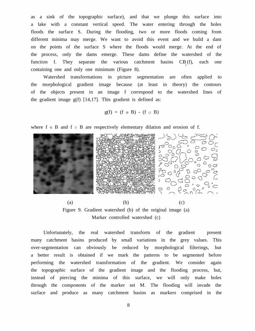
Watershed transformations in picture segmentation are often applied to

the morphological gradient image because (at least in theory) the contours

of the objects present in an image f correspond to the watershed lines of

the gradient image g(f) [14,17]. This gradient is defined as:

g(f) = (f s B) - (f x B)

where f s B and f x B are respectively elementary dilation and erosion of f.

(a) (b) (c)

Figure 9. Gradient watershed (b) of the original image (a)

Marker controlled watershed (c)

Unfortunately, the real watershed transform of the gradient present

many catchment basins produced by small variations in the grey values. This

over-segmentation can obviously be reduced by morphological filterings, but

a better result is obtained if we mark the patterns to be segmented before

performing the watershed transformation of the gradient. We consider again

the topographic surface of the gradient image and the flooding process, but,

instead of piercing the minima of this surface, we will only make holes

through the components of the marker set M. The flooding will invade the

surface and produce as many catchment basins as markers comprised in the

8

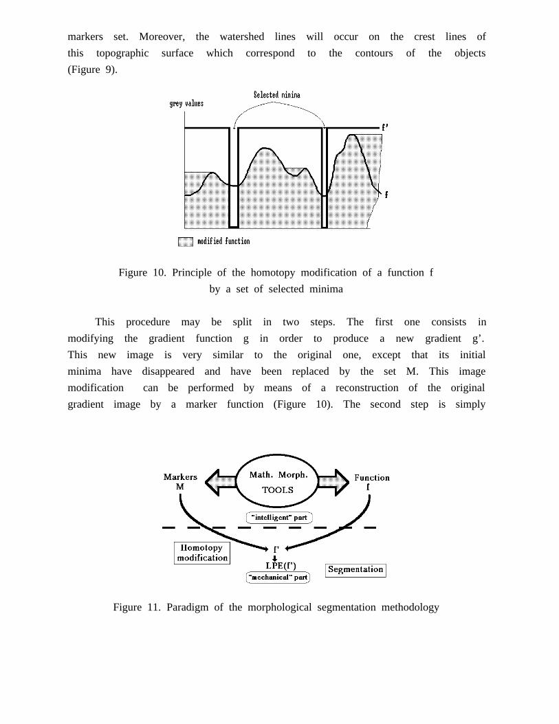
markers set. Moreover, the watershed lines will occur on the crest lines of

this topographic surface which correspond to the contours of the objects

(Figure 9).

Figure 10. Principle of the homotopy modification of a function f

by a set of selected minima

This procedure may be split in two steps. The first one consists in

modifying the gradient function g in order to produce a new gradient g’.

This new image is very similar to the original one, except that its initial

minima have disappeared and have been replaced by the set M. This image

modification can be performed by means of a reconstruction of the original

gradient image by a marker function (Figure 10). The second step is simply

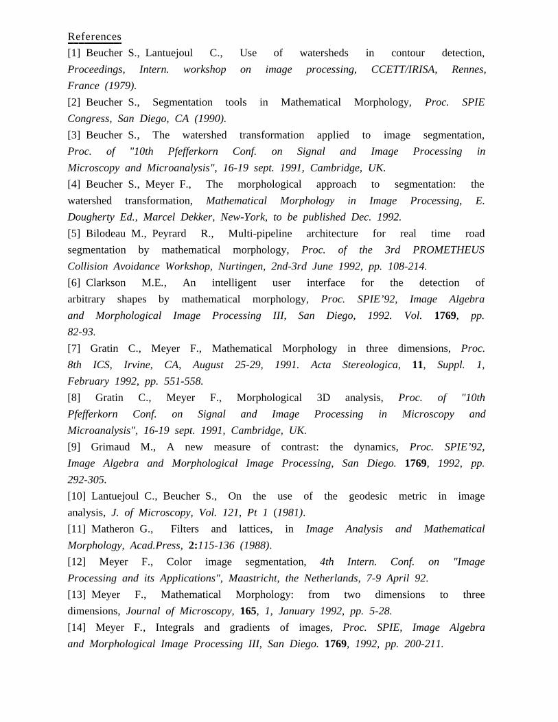
Figure 11. Paradigm of the morphological segmentation methodology

the watershed construction of g’. This approach leads to a general

meyhodology of the segmentation consisting in selecting first a markers set

M pointing out the objects to be extracted, then a function f quantifying a

segmentation criterion (this criterion can be, for instance, the changes in

grey values). This function is modified to produce a new function f’ having

as minima the set of markers M. The segmentation of the initial image is

performed by the watershed transform of f’. The segmentation process is

therefore divided in two steps: an "intelligent" part whose purpose is the

determination of M and f, and a "straightforward" part consisting in the use

of the basic morphological tools which are watersheds and image modification

(Figure 11). A lot of segmentation problems may be solved according to this

general scheme [14].

II) New algorithms and new processors====================================================================================================================================================================

Designing new morphological tools is helpful as soon as the computation

time for achieving these transformations is not too long. Two solutions

exist for improving the computation speed: a hardware solution, consisting

in using efficient morphological processors, and a software solution, that

is finding new and fast algorithms. These two approaches may be closely

linked and very often, good software algorithms are sooner or later

implemented into hardware.

II-1) New algorithms=======================================================================

Some algorithms already exist which highly increase the effectiveness

of some morphological tools. For instance, the recursive algorithms allow to

build very quickly the distance function and the geodesic distance function

of a set. These functions provide euclidean and geodesic erosions and

dilations in a time which is not proportional to their size.

Unfortunately, it is not possible to obtain greytone erosions and

dilations by this means because there exists no equivalent of the distance

function for a greytone image. However, the recursive algorithms can be used

both on binary and greytone images for the reconstruction transformation.

II-1-1) Recursive algorithms=============================================================================================

The principle of a recursive algorithm is to transform any point x

of an image by using its neighbourhood already transformed points. The

computation speed is dramatically increased because of the propagation of

the transformation in the image. As an illustration, take the algorithm for

the recursive reconstruction of a function f by a marker function g. For any

10

point x of f, the new value of f is given by:0

f(x ) = Inf [g(x ), Sup [f(x ),f(x ),f(x ),f(x )]]0 0 0 1 2 3

on the hexagonal grid and in the first step. Then, in the second step, the

value of f at point x becomes:0

f(x ) = Inf [g(x ), Sup [f(x ),f(x ),f(x ),f(x )]]0 0 0 4 5 6

x x1 2

x x x3 0 6

x x5 4

The process is repeated, in the direct and reverse scanning order of

the image until idempotence. For most pictures, this idempotence is reached

in less than five scans (Figure 12).

Figure 12. Recursive reconstruction of a function by another function

II-1-2) Speeding up the watershed=========================================================================================================================

Many algorithms have been designed for speeding up the watershed

construction. Some of them use the already existing architecture of the

morphological processors and simply try to reduce the number of flooded

levels by using mathematical anamorphosis. Although they produce a slight

loss of information, in most cases, they are of a great help, especially

when dealing with scene analysis. Other algorithms producing true watershed

and true marker-controlled watershed have also been designed. Among them,

one can distinguish between the procedures which simulate the flooding

process and the algorithms which try to directly extract the watershed

lines. In the first group, the algorithm using ordered queues are very

attractive.

During the flooding of a topographic surface, there appears a dual

order relation between the pixels (we consider here the flooding with

sources placed at the regional minima or the function). It is clear that a

point x is flooded before a point y if y is higher than x on the relief.

This constitutes the first level of the hierarchy. It is simply the order

relation between the grey values. A second order relation occurs on the

plateaus. Let X be a plateau at an altitude h. Before X begins to be flooded

all neighboring points of X, with a lower altitude than h have been flooded.

One supposes that the flooding of the plateau is not instantaneous but

progressive. The flood progresses inwards into the plateau with uniform

speed. The first neighbors of already flooded points are flooded first.

Second neighbors are flooded next, etc.. This introduces a second order

relation among points with the same altitude, corresponding to the time when

they are reached by the flood. If two points x and y belong to the same

plateau X, of height h, x will be reached by the flow before y if the

geodesic distance within the plateau X to the points of lower altitude is

smaller for x than for y. An ordered queue naturally introduces this

hierarchical order relation. Implementing an ordered queue between the

pixels of an image leads to reconstruction and watershed algorithms which

are very fast because every point is treated one time as clients in a queue.

The complete description of the watershed algorithm using an ordered queue

would be to long to explain in the scope of this paper. Refer to [4] for

further information.

In the second group, one can find algorithms which use a special

representation of the image: the arrowing representation [2].2From f : Z L Z, we may define an oriented graph whose vertices are the

2points of Z and with edges or arrows from x to any adjacent point y iff

f(x) < f(y) (Figure 13).

The definition does not allow the arrowing of the plateaus of the

topographic surface. This arrowing can be performed by means of geodesic

dilations. The operation is called the completion of the arrows graph.

Moreover, in order to suppress problems due to the fact that a watershed

line is not always of zero thickness, a more complicated procedure called

over-completion is used, which leads to a double arrowing for some points.

Then, starting from this complete graph (over-completed), we may select some

configurations which, locally, correspond to divide lines. These

12

configurations are represented on Figure 14 for the 6-connectivity

neighborhood of a point on a hexagonal grid (up to a rotation).

Figure 13. Function f and its complete graph of arrows

Any point receiving arrows from more than one connected component of

its neighborhood may be flooded by different lakes. Consequently, this point

may belong to a divide line. In a second step, the arrows starting from the

selected points must be suppressed. These points, in fact, cannot be

flooded, so they cannot propagate the flood. Doing so, we change the

arrowing of the neighboring points and consequently the graph of arrows.

Provided that the over-completion of this new graph has been made, some new

divide points may then appear. The procedure is re-run until no new divide

point is selected (Figure 15).

1 0 1 0 1 1 1 1\ \ \ / \ /> > > M > M0 0 J----------1 0 0 0 0 0 0 0 0 0

U U O\ \ /0 0 0 1 0 1 1 0

1 1 1 1\ / \ /> M > M0 0 J----------1 0 0 0O O U

/ / \1 0 1 1

Figure 14. Configurations of arrows corresponding

to possible divide points (hexagonal grid)

This algorithm produces local watershed lines. The true divide lines

can be extracted easily; they are the only ones which form closed curves.

Figure 15. Watershed by arrowing: primary divide points (left)

final result (right)

II-2) Morphological processors================================================================================================================

A classical morphological processor is made of a neighbourhood logic

which allows to compute basic morphological transformations with elementary

structuring elements. As a matter of fact, the higher the speed of this

elementary logic, the higher the overall performances of the whole system.

The latest morphological processors obviously include this elementary logic,

both for binary and greytone images but also a large set of capabilities in

the field of geodesic transformations. The most recent developments in the

area of morphological processors have materialized into an ASIC named PIMM1,

an acronym for Integrated Mathematical Morphology Processor [15]. This

integrated circuit designed at the CMM is a complete morphological processor

for greytone and binary images of any size. The neighbourhood logic enables

treatments on a square or hexagonal grid. This chip also contains a

recursive logic for the fast computation of distance functions and for fast

binary reconstructions. It has some capabilities of arrowing and an

arithmetic logic allows the use of anamorphosis to reduce the computation

time of the watershed.

However, many algorithms are not implemented in this chip, in

particular greytone reconstruction and hierarchical queues. Nevertheless,

the fact that it can be pipelined allows to design architectures which meet

the needs of real-time processing. Some realizations are pending at the CMM,

their final goal is to segment macroscopic images in real-time (that is in a

few hundred milliseconds).

14

III) New areas of application===================================================================================================================

III-1) Greytone morphology===============================================================================================

For many people, MM is par excellence a methodology for binary 2D

images. This is definitely inadequate. Nowadays, MM is mainly used with

greytone images because they are typically the kind of images we find in the

real world. Moreover the result obtained when dealing with greytone images

are often better than those available with binary morphology because the

loss of information when transforming pictures is better controlled. At the

beginning of MM, two areas of application existed: the material sciences and

the biomedical area. In both cases, pictures were mainly microscopic ones

and the main purpose of MM was to quantify the structures. Now, new fields

of application appear, especially in the macroscopic world. Many image

processing problems in scene analysis (Figure 16) and industrial vision have

been solved with the help of MM [16,21,23]. With the development of refined

sensors in radiology, it is now possible to extract fuzzy features from the

Figure 16. Examples of watershed segmentation of trafic pictures

Lanes segmentation (upper), road segmentation (lower)

images in medical radiology (micro-calcifications for instance in the early

screening of cancer) or in non destructive industrial inspection (defect

detection in aircraft engines).

In electron microscopy also, MM is helpful [3]. First, many electron

microscopes are directly connected to an image analyzer and second, the new

tools of MM, particularly in the filtering process, are very efficient

(Figure 17).

Figure 17. Segmentation of grains in TEM images, two examples

III-2) From 2D to 3D========================================================================

A major advantage of MM is its straightforward extension from the 2D

domain to 3D [7,8,13]. Almost, all the morphological tools which have been

designed for 2D pictures can be directly used in 3D. It is the case for

basic operations (erosions, dilations, openings, closings and so on) but

also, and it is the great advantage of MM, for the more complex ones such

picture reconstruction, watersheds, skeletons... . As a consequence, MM

provides, in the 3D domain, efficient tools for image quantification and

segmentation. Moreover, the extension of MM to 3D greytone images is

16

possible. This capability is widely used to process images delivered by many

new sensors in tomography, NMR, confocal microscopy, holography, etc..

(Figure 18). Another interesting application of 3D morphology is given by

motion images. A sequence of images can be considered as a 3D picture and

processed as such by MM. The results are very interesting because the

topological relationships between the different objects in the scene are

preserved both in the spatial domain and in the temporal domain.

Figure 18. Segmentation of a 3D holographic picture of droplets (section)

III-3) Multi-spectral images================================================================================================

MM can be used with multi-spectral images. The main source for such

images is remote sensing and color images. Practical problems may arise when

dealing with such images but also theoretical ones. In fact, contrary to

greytone images where basic morphological transformations have a physical

meaning, it is not the case for color images: what could be the definition

and meaning of a color image erosion? The main reason of this difficulty is

that it is not possible to define arbitrarily an order relation between the

pixels in a color image (there is no underlying lattice). For that reason,

when working with multi-spectral images, one must first build this order

relationship according to the problem under study. For instance, in a color

image, if you are interested in the red objects, you will build, starting

from the original image, a new greytone image where the red pixels will be

the lightest ones. Then, the whole set of MM tools will be available for

analyzing this new images (Figure 19) [12].

Figure 19. Example of color segmentation: the segmentation (right)

allows to simplify the original image (left)

The future of MM=====================================================================================

In twenty years, MM, which was considered as an "exotic" technique has

become a complete methodology for image processing. It is no longer possible

now to work with an image analyzer which is not equipped with morphological

tools together with linear image processing tools. The latest developments

undoubtedly show the fast emergence of real-time processors used in many new

fields where they are indispensable: scene analysis, robotics control, video

image compression and restoration, image communication, etc.. [5]. If the

increase of computation speed allows to use more and more complex tools, the

major problem which may arise for the end-user is to learn how to use these

tools. Solving any image application by MM needs to concatenate thousands of

elementary operations and it is not a simple task to catch in the MM toolbox

the most efficient operators. For that reason, it is of primary importance

to provide with the fast processors efficient programming languages. Image

analysis in general, and MM in particular, are areas where the available

language for translating your ideas in terms of a program must be well

matched. Many efforts are made in this field, especially in the direction of

"threaded" and object oriented languages. Moreover, in order to give the

end-user morphologist a quick and easy know-how, techniques of artificial

intelligence are presently developed to help him to select among the various

available tools those which can be useful to solve his problem [6,20]. It is

a fact that MM transformations are well adapted to this approach. The

marker-controlled segmentation for instance is a good example of a

methodology where AI can be used.

18

References=================================================

[1] Beucher S., Lantuejoul C., Use of watersheds in contour detection,

Proceedings, Intern. workshop on image processing, CCETT/IRISA, Rennes,

France (1979).

[2] Beucher S., Segmentation tools in Mathematical Morphology,Proc. SPIE

Congress, San Diego, CA (1990).

[3] Beucher S., The watershed transformation applied to image segmentation,

Proc. of "10th Pfefferkorn Conf. on Signal and Image Processing in

Microscopy and Microanalysis", 16-19 sept. 1991, Cambridge, UK.

[4] Beucher S., Meyer F., The morphological approach to segmentation: the

watershed transformation,Mathematical Morphology in Image Processing, E.

Dougherty Ed., Marcel Dekker, New-York, to be published Dec. 1992.

[5] Bilodeau M., Peyrard R., Multi-pipeline architecture for real time road

segmentation by mathematical morphology,Proc. of the 3rd PROMETHEUS

Collision Avoidance Workshop, Nurtingen, 2nd-3rd June 1992, pp. 108-214.

[6] Clarkson M.E., An intelligent user interface for the detection of

arbitrary shapes by mathematical morphology,Proc. SPIE’92, Image Algebra

and Morphological Image Processing III, San Diego, 1992. Vol.1769, pp.

82-93.

[7] Gratin C., Meyer F., Mathematical Morphology in three dimensions,Proc.

8th ICS, Irvine, CA, August 25-29, 1991. Acta Stereologica,11, Suppl. 1,

February 1992, pp. 551-558.

[8] Gratin C., Meyer F., Morphological 3D analysis,Proc. of "10th

Pfefferkorn Conf. on Signal and Image Processing in Microscopy and

Microanalysis", 16-19 sept. 1991, Cambridge, UK.

[9] Grimaud M., A new measure of contrast: the dynamics,Proc. SPIE’92,

Image Algebra and Morphological Image Processing, San Diego.1769, 1992, pp.

292-305.

[10] Lantuejoul C., Beucher S., On the use of the geodesic metric in image

analysis,J. of Microscopy, Vol. 121, Pt 1(1981).

[11] Matheron G., Filters and lattices, inImage Analysis and Mathematical

Morphology, Acad.Press,2:115-136 (1988).

[12] Meyer F., Color image segmentation,4th Intern. Conf. on "Image

Processing and its Applications", Maastricht, the Netherlands, 7-9 April 92.

[13] Meyer F., Mathematical Morphology: from two dimensions to three

dimensions,Journal of Microscopy,165, 1, January 1992, pp. 5-28.

[14] Meyer F., Integrals and gradients of images,Proc. SPIE, Image Algebra

and Morphological Image Processing III, San Diego.1769, 1992, pp. 200-211.

[14] Meyer F., Beucher S., Morphological segmentation,Journal of Visual

Communication and Image representation,1.1:21-45 (1990).

[15] Peyrard R., Klein J-C., Speeding up Mathematical Morphology processes

by using a new ASIC: PIMM1, Proc. Computer Architecture for Machine

Perception - CAMP 91, Paris 16-17 December 1991, ETCA/CNRS, IEEE/AFCET, pp.

439-452.

[16] Rivest J-F., Beucher S., Delhomme J-P., Marker-controlled segmentation:

an application to electrical borehole imaging, Journal of Electronic

Imaging, 1, 2, April 1992, pp. 136-142.

[17] Rivest J-F., Soille P., Beucher S., Morphological gradients,Proc. SPIE

"Image Science and Technology", San Jose, California, Feb. 9-14, 1992. 12 p.

[18] Serra J., Image Analysis and Mathematical Morphology, Vol.2,

Theoretical Advances ,Academic Press, London(1988).

[19] Serra J., Vincent L., An Overview of Morphological Filtering,Circuits

Systems & Signal Processing,11, 1, 1992, pp. 47-108.

[20] Schmitt M., Mathematical Morphology and Artificial Intelligence: an

automatic programming system, Signal Processing, special issue on

Mathematical Morphology, Vol. 16, n˚ 4, April 1989.

[21] Talbot H., Jeulin D., Hobbs W., Scanning Electron Microscopy image

analysis of fiber glass insulation, Proc. 50th Annual Meeting of the

Electron Microscopy Society of America, Boston, 16-21 August 1992 (G.W.

Bailey et al. Eds). 1992, pp. 994-995.

[22] Vincent L., Soille P., Watersheds in digital spaces: an efficient

algorithm based on immersion simulations,IEEE PAMI, 1.6:583-597 (1990).

[23] Yu X., Beucher S., Bilodeau M., Road tracking, lane segmentation and

obstacle recognition by mathematical morphology, Proc. Intelligent

Vehicles’92 Symposium, June 29-July 1, 1992, Detroit, pp. 166-170.

20