Recent Advances in Modeling Liquidity Risk and Applications to Central Clearing

Marco Avellaneda

New York University and

Finance Concepts LLC

Global Derivatives USA, November 20, 2013

Outline

• Liquidity in risk management: listed markets, OTC Markets

• Liquidity-adjusted VaR for directional exposures • BM&F Bovespa’s Close-out Risk Evaluation (CORE) • Modeling Liquidity Charges in OTC Markets & Liquidity Polls

Importance of Liquidity Modeling

• Need to go beyond VaR. In most cases, VaR is grossly insufficient due to prolonged, expensive liquidation. • LTCM (1998): basis trades (long high spreads/short low spreads, DV01=0)

• Credit Crunch (2007, 2008): loss of liquidity for financing MBS, ABS and Credit Derivatives • J.P. Morgan CIO (2012): basis trade, index CDS versus corporate CDS (2bb loss -> 8 bb loss)

• MF Global (2012): 2y term repos on Italian government bonds • Grupo Interbolsa (2012) : Fabricato share repos, collapse of 2nd largest Colombian broker-dealer

Main Themes in Liquidity Modeling

Liquidity = the ability to convert a given position into cash or risk-less securities

• Size matters:

The larger the quantity, the worst is the outcome. p=1.5 is generally accepted, but there exists some controversy among academics, e.g. Gabaix p=0.5, Cont p=1 • Time-horizon matters: there is a maximum reasonable amount of inventory that can be liquidated in a given period of time (Almgren & Chriss, 2000). Break large orders into smaller pieces (TWAP, WVAP, PoV) • Market structure matters: OTC derivatives markets have different price/liquidity discovery properties than listed markets.

∆𝑃 = 𝐶𝑜𝑛𝑠𝑡.× 𝑄 𝑝

Differences between OTC and Listed Markets

• In exchanges, liquidity models are based on daily trading volumes, open interest and bid-ask spreads. • In over-the-counter (OTC) markets, trades and volumes are unknown and post-trade/market depth data are not easy to find (Avellaneda and Cont, 2010). • Main challenge: to calculate suitable liquidity reserves or ``charges ‘’ for portfolios. • This problem is directly relevant to central counterparty clearing of derivatives and portfolio risk-requirements in the post-2008 era. In CCPs, liquidity must be modeled explicitly.

Liquidity-adjusted VaR: simple exercise or complex calculation?

T+1 T+2 T+3

Initial jump modeled by Var/ES/CVaR (``market risk’’)

Large size implies further loss due to market impact

PNL

Heuristics: Liquidity Curves

𝐿 𝑄 =a× 𝑄 1.5

𝐿𝑉𝑎𝑅 𝑄 ∙ 𝑋 = 𝑉𝑎𝑅 𝑄 ∙ 𝑋 + 𝑎 𝑄 1.5

Good for ``outright’’ positions. Not good for portfolios, where we have offsets between long and short positions in instruments with common RFs

T+1 T+2 T+3

PNL

Liquidity Charge

Simple liquidity model 𝑄 = notional quantity 𝑄0= ``typical’’ trade size 𝜎 = price volatility (%) 𝑁 = 𝑄/𝑄0 dimensionless size of the position 𝜉𝑖 = iid Student-t r.v. mean=0, variance=1, df >2

𝑃𝑁𝐿 𝑛 = 𝜎(𝑄 − 𝑖𝑄0)𝜉𝑖

𝑛

𝑖=1

= 𝜎𝑄 𝑁 1−𝑖

𝑁

𝜉𝑖

𝑁

𝑛

𝑖=1

= 𝜎𝑄0𝑄

𝑄0

1.5

1−𝑖

𝑁

𝜉𝑖

𝑁

𝑛

𝑖=1

≈ 𝜎𝑄0𝑄

𝑄0

1.5

1 − 𝑡 𝑑𝑊𝑡

𝜏

0

𝑁, 𝑛 ≫ 1, 𝑛/𝑁 → 𝜏

Liquidity Add-on?

• Scaling gives a PNL for liquidation which is a standardized stochastic process (stochastic integral) multiplied by a nonlinear function of quantity. • Any risk-measure (e.g. VaR, CVaR, STDEV) will give rise to a liquidation cost of the form • This is the asymptotics for large Q. Therefore, the LC should be something like this

𝑃𝑁𝐿 = 𝜅 𝜎 𝑄0𝑄

𝑄0

1.5

= 𝜅 𝜎𝑄1.5

𝑄00.5

𝐿𝐶(𝑄) = 𝜅 𝜎 𝑄0𝑚𝑎𝑥𝑄

𝑄0

1.5

,𝑄

𝑄0 𝜅𝜎 ≅

1

2 (bid-ask spread)

Example: Eurodollar Futures

• CME ED Futures: Median Volume ~ 100 K contracts • Tick size (and bid/ask spread)= 0.25 bps for front month, 0.5 bps others.

• Contract sensitivity = USD 25 per LIBOR basis point move • Reasonable volume = 10% daily volume = 10,000 contracts • Typical liquid (large) trade = 10,000× 25 = 250,000 USD of DV01

Deriving Liquidity Curves

LC(X) = 1

2 s ×

𝑋

𝑋0

1.5

• Liquidity Charge for normal trades= ½ bid-ask spread Front month = 1/8 basis point Out months = ¼ basis point

𝐿𝐶𝑓 𝑋 = (0.125)𝑋

0.25

1.5=𝑋1.5

𝐿𝐶𝑏 𝑋 = (0.25)𝑋

0.25

1.5=2 𝑋1.5

DV01

spread 1 MM 5 MM 10 MM 25 MM

0.25 1 11 32 125

0.5 2 22 63 250

1 4 45 126 500

Liquidity charges in basis points of notional For different sizes measured in MM Dv01

Market and Liquidity Risk for Portfolios

Central clearing & risk-management

CM1

CM2

CM3

CM4

CM5

CM6 CM7

CCP

Large circles: Clearing members (large banks, BDs) Small circles: non-clearing market participants (buy side) Arrows represent credit exposure

Major Clearinghouses Today

Inter-bank payments: ACH Securities: DTCC, FICC, LCH.Clearnet, Eurex Clearing Derivatives: CME Group, LCH.Clearnet, Intercontinental Exchange (ICE), ICE Clear Europe, Eurex Clearing, Hong-Kong Exchanges and Clearing Equity Options: The Options Clearing Corporation In Brazil, BM&F Bovespa manages 4 CCPs for different asset classes (like CME Group, which clears commodities, financials, and some OTC)

Tools for Risk Management of CCPs

• Initial Margin (Market Risk, Liquidity Risk)

• Fund for mutualization of losses (``Guarantee Fund’’), covering shortfall beyond the IM • ``Loss tranches’’ with CCP’s own capital ( Skin in the game)

BIS, Principles for Financial Markets Infrastructures, BIS CPSS-IOSCO Consultative Report, April 2012 ESMA, Final Report, Technical Standards on OTC Derivatives, CCPs and Trade Repositories (``EMIR’’), September 2012

Some CCP Risk-management issues which combine market and liquidity risk

• How can the CCP remain well-capitalized during the liquidation of a defaulted participant? • Create synergies by using a common system to clear different products with the same risk factors (e.g. listed and OTC derivatives, collateral-in-margin)? • How to handle a portfolio of securities sensitive to the same risk-factors but having different liquidity ? • Treat portfolios which have daily settlement (futures) as well as OTC securities (forwards) which do not have daily settlement?

Close Out Risk Evaluation (CORE)

Close-Out Risk Evaluation (CORE) proposed by BM&F Bovespa

• Find a suitable liquidation strategy for each participant’s portfolio • Compute potential uncollateralized losses associated with liquidation of the portfolio under stress scenarios • Margin requirement is based on potential losses over the liquidation period

BM&FBOVESPA’s Post-Trade Infrastructure: Integration Opportunities and Challenges, September 2010, www.bmf.com.br/bmfbovespa/pages/boletim2/informes/2010/marco/WhitePaper.pdf

Example 1: Liquid vs. illiquid stock

Petrobras average trading volumes PETR4: 24 million shares/day ( assume max liq. =3MM ) PETR3: 8 million shares/day ( ‘’ =1MM ) Portfolio: Long 40 MM PETR4, short 30MM PETR3

PETR4 (sell)

PETR3 (buy)

1

1

3 3 3 3 3 1 1 1 1 1 1 1 1 ------------------------ 1 1 1 1 1 1

1 1 1 1 1 1 1 1 1 1 1 1 ------------------------ 1 1 1 1 1 1

Day 5 30

Mkt. exposure: 10 MM PETR4 for 5 days PETR 4 ``hedges’’ PETR 3 MTM P/L during liquidation

Liquidating independently of common risk factors (naïve liquidation)

PETR4 (sell)

PETR3 (buy)

1

1

3 3 3 3 3 3 3 3 3 3 3 3 3 1 0 0------------------------ 0 0 0

1 1 1 1 1 1 1 1 1 1 1 1 1 1 1------------------------ 1 1 1

Day 5 30

Mkt. exposure: 26 MM PETR4 for first 13 days, 16 MM PETR3 for last 15 days Much more market risk than previous example. Naïve liquidation always costs more. Some optimization can be done.

14

Example 2: portfolio of futures and OTC forwards with bond collateral

Portfolio: Long 10,000,000 BRL in USD futures (liquid) Short 10,000,000 BRL in forwards (illiquid, with auction in 10 days) Long 20,000,000 in Brazilian T-bills (LTN) (liquid, but not cash)

Naïve Strategy #1: • Close futures position, sell T-bills, wait 10 days with the forward position

Naïve Strategy #2: • Do not close futures position, wait 10 days with forward position, then sell T-bills

Correct strategy takes into account daily settlement of futures

Best strategy: • Do not close futures position, wait 10 days with forward position, Sell a fraction of T-Bills to cover variation margin in Futures for 10 days. Close the remaining portfolio in 10 days

20

10

-10

20

10 20

Naïve #1

Naïve #2

Best strategy

(may require more collateral)

Modeling portfolios with liquidity constraints

• In a world with infinite liquidity, a portfolio is represented as a list of instruments and quantities • In a world with limited liquidity, we should include the maximum amounts that can be traded in a given period (day) without `moving the market’*

* Proxied here at 10 % Avg. Traded Volume ** Guararapes Confecc. SA

Portfolio Description

• R represents the state of the market or path of states of the market (risk-factor changes)

• Example: if we are dealing with options, then 𝑅𝑡 =

𝑆𝑡𝜎𝑡𝑟𝑡𝑑𝑡

• represent quantities and daily liquidity limits for each instrument

𝑹 = 𝑅0, 𝑅1, 𝑅2, …𝑅𝑡 , 𝑅𝑡+1, …

Und. Price Volatility Interest rate Dividend yield

The Risk-factors

𝑄𝑖,𝑙𝑖

Liquidation of a Portfolio: `Close-out strategy’

• On date t=0, you decide that a portfolio should be liquidated starting on t=1. • Determine a strategy in which a certain fraction, 𝑞𝑖𝑡, of the of the position in instrument i will be liquidated at date t. ( 𝑞𝑖𝑡 , 𝑖 = 1,… , 𝑁, 𝑡 = 1,… , 𝑇𝑚𝑎𝑥)

• A close-out strategy is a matrix that tells us how to proceed for liquidating the various instruments in the portfolio as time passes.

0 ≤ 𝑞𝑖𝑡 ≤𝑙𝑖

𝑄𝑖≡ 𝑘𝑖 ∀𝑖 ∀𝑡

𝑞𝑖𝑡 = 1

𝑇𝑚𝑎𝑥

𝑡=1

𝑛𝑡 = 𝑞𝑠

𝑇𝑚𝑎𝑥

𝑠=𝑡+1

The remaining balance (%) at time t

Defining the objective function: Profit and loss of a close-out strategy for a portfolio

𝜓𝑖 𝑡, 𝑅𝑡 ≝ 𝑄𝑖 𝑀𝑇𝑀𝑖 𝑡, 𝑅𝑡 −𝑀𝑇𝑀𝑖 0, 𝑅0

• Realized P/L at date t, after trading

• Unrealized (a.k.a. MTM) P/L at date t, after trading

𝐿𝑟 𝑡, 𝑞, 𝑅𝑡 = 𝑞𝑖𝑡𝜓𝑖 𝑡, 𝑅𝑡

𝑁

𝑖=1

P/L, full valuation

𝐿𝑛𝑟 𝑡, 𝑞, 𝑅𝑡 = 𝑛𝑖𝑡𝜓𝑖 𝑡, 𝑅𝑡

𝑁

𝑖=1

Accumulated P/L

• Accumulated profit/Loss for close out strategy at date t

𝐿 𝑡, 𝑞, 𝑅 = 𝐿𝑟 𝑠, 𝑞, 𝑅𝑠

𝑡

𝑠=1

+ 𝐿𝑛𝑟 𝑡, 𝑞, 𝑅𝑡

= 𝑞𝑖𝑠𝜓𝑖 𝑠, 𝑅𝑠

𝑁

𝑖=1

𝑡

𝑠=1

+ 𝑛𝑖𝑡𝜓𝑖 𝑡, 𝑅𝑡

𝑁

𝑖=1

cash unrealized gain/loss

CORE objective function

• Define scenarios for the risk-factors, 𝑅 = 𝑅1, 𝑅2, … , 𝑅𝑇𝑚𝑎𝑥

• These scenarios are paths. Let 𝑹 denote the set of all scenarios considered

𝑈 𝑞 = min

𝑅∈𝑹min1≤𝑡≤𝑇𝑚𝑎𝑥

𝐿 𝑡, 𝑞, 𝑅

= min𝑅∈𝑹min1≤𝑡≤𝑇𝑚𝑎𝑥

𝑞𝑖𝑠𝜓𝑖 𝑠, 𝑅𝑠

𝑁

𝑖=1

𝑡

𝑠=1

+ 𝑛𝑖𝑡𝜓𝑖 𝑡, 𝑅𝑡

𝑁

𝑖=1

The Optimization Problem

Maximize Subject to:

𝑈 𝑞 𝑞 = 𝑞𝑖𝑡 ∈ 𝑅𝑁×𝑇𝑚𝑎𝑥

0 ≤ 𝑞𝑖𝑡 ≤𝑙𝑖

𝑄𝑖≡ 𝑘𝑖 ∀𝑖 ∀𝑡

𝑞𝑖𝑡 = 1

𝑇𝑚𝑎𝑥

𝑡=1

∀𝑖

• U(q) is a sum of minima of linear functions of q => it is concave • The set of constraints is convex (it is a convex polyhedral region)

A solution exists and should be unique under reasonable conditions!

Solution Via Linear Programming for 𝑈2

Maximize: Variables: Subject to constraints:

𝑈

𝜆𝑡 ≤ 𝑞𝑖𝑡𝜓𝑖 𝑡, 𝑅𝑡 ∀𝑡 ∀𝑅 ∈ 𝑹

𝑁

𝑖=1

𝑈, 𝜆𝑡, 𝜇𝑡 , 𝑞𝑖𝑡; 1 ≤ 𝑡 ≤ 𝑇𝑚𝑎𝑥, 1 ≤ 𝑖 ≤ 𝑁

𝜇𝑡 ≤ 𝑞𝑖𝑡 + 𝑛𝑖𝑡 𝜓𝑖 𝑡, 𝑅𝑡 ∀𝑡 ∀𝑅 ∈ 𝑹

𝑁

𝑖=1

0 ≤ 𝑞𝑖𝑡 ≤𝑙𝑖

𝑄𝑖≡ 𝑘𝑖 ∀𝑖 ∀𝑡

𝑞𝑖𝑡 = 1

𝑇𝑚𝑎𝑥

𝑡=1

∀𝑖

𝑈 ≤ 𝜆𝑡 + 𝜇𝑡 ∀𝑡

BMF-CORE Liquidity Adjusted Risk Margin

𝑀 = max𝑞min𝑅𝜖𝑹

min1≤𝑡≤𝑇𝑚𝑎𝑥

𝐿 𝑡, 𝑞, 𝑅

= min

𝑅𝜖𝑹min1≤𝑡≤𝑇𝑚𝑎𝑥

𝐿 𝑡, 𝑞∗, 𝑅

• Alternative versions, which can be used with Monte Carlo models for RFs,

𝑉𝑎𝑅𝛼 min1≤𝑡≤𝑇𝑚𝑎𝑥

𝐿 𝑡, 𝑞∗, 𝑅 𝛼 = .99, 𝑜𝑟 .995

𝐸𝑆𝛼 min1≤𝑡≤𝑇𝑚𝑎𝑥

𝐿 𝑡, 𝑞∗, 𝑅 𝛼 = .99…

𝑞∗ = optimal close-out strategy

Example: Liquidation of a portfolio of stocks using the CORE risk-measure and Historical Monte Carlo

• 10 stocks, 100 shares per stock

SPY GDX UVXY VTI VWO SIL TLT IWM AGG VOO

𝐸𝑆 𝑋, 𝑇 = 𝐸𝑆.99 min𝑡≤𝑇𝐿(𝑡, 𝑞, 𝑅)

Strategy q: liquidate equal amounts of stocks each day (not optimal)

1 day ES(99)

Portfolio Liquidity Modeling in OTC Markets

Liquidity in OTC Risk-Management

• In OTC risk-management, the portfolio is liquidated in an auction (there is not exchange). • Participants periodically inform the CCP on liquidity and market depth, so IM requirements can take into account liquidation costs. • Difficulties may arise since the ex-ante liquidation costs used for risk management are provided by agents which will bid on the defaulted portfolio at auction (ex-post).

• The time dimension of liquidation should be ``made equivalent’’ to a wider B/O spread in a 1-day auction. .

Polling

• Polls are conducted asking CCP participants by how much would their bid or ask price change as a function of trade size

• Liquidity polls typically involve

-- directional positions -- market-neutral portfolios • Liquidity charges for market-neutral portfolios are typically lower than for outright positions because they have less risk exposure • To some extent, the poll incorporates the time-dimension of the close-out process

Example: Swaps

• We consider 4 standard swap tenors. A typical poll will consider several portfolios: outright swap positions, curve positions (or time spreads) and butterfly spreads. Portfolios 5 to 13 are market-neutral.

Swap positions (in MM DV01)

Tenor (yrs) 2 5 10 30

Port 1 1

Port 2 1

Port 3 1

Port 4 1

Port 5 1 -1

Port 6 1 -1

Port 7 1 -1

Port 8 1 -1

Port 9 1 -1

Port 10 1 -2 1

Port 11 1 -2 1

Port 12 1 -2 1

Port 13 1 -2 1

Liquidity Charge Curves obtained by polling 10 dealers and taking median values

• We use the median value as an indicator of the function F(N) for each spread • Rows 1 and 2 are similar to what we obtained earlier for ED futures based on 1.5 model

Portfolio multiplier (1X, 5X,10X,25X)

1 5 10 25

1 1.25 17.50 60.00 237.50

2 1.93 20.00 70.00 250.00

3 2.25 25.00 80.00 337.50

4 3.00 30.00 100.00 450.00

5 1.00 12.50 45.00 168.75

6 2.00 18.18 60.00 212.50

7 2.00 20.61 80.00 275.00

8 2.00 15.00 47.50 187.50

9 2.00 20.00 60.00 253.13

10 2.00 20.00 80.00 -

11 2.00 30.00 80.00 -

12 4.00 40.00 150.00 -

13 4.00 40.00 135.00 -

Smoothing the Poll Data • Take the discrete poll and fit the data to power-laws using log-log regression

bps

MM DV01

Outright 2Y swap

𝐹 𝑁 =(1.26827)*𝑁1.6406

Bps for 1MM DV01

Exponent greater Than 1

Empirical results for LCCs

Liquidity Add on Charge Calculation for IR Swap Portfolios

• Represent swap portfolios as loadings on the standard tenor swaps (2y,5y,10y,30y)

• Minimize:

subject to the linear constraints and bound constraints

𝐹𝑖 𝑄𝑖

𝑁

𝑖=1

𝜇𝑖𝑚𝑄𝑖 = ∆𝑚

𝑁

𝑖=1

𝑚 = 1,… ,𝑀

𝑄𝑖 ≤ 𝑄𝑚𝑎𝑥,𝑖 i= 1,… ,𝑁

Example TARGET PORTFOLIO (in MM DV01)

TENOR 2 5 10 30

DV01 MM 12 -18 5 -5

CHARGE (bps) 74.78 155.15 22.01 34.26

NAÏVE CHG 286.20

CALCULATED CALCULATED

SPREAD HEDGE POSITION LIQUIDITY CHARGE

1 0.00 0.00

2 -0.46 0.59

3 0.33 0.38

4 -5.86 43.86

5 17.72 101.57

6 -4.64 18.14

7 -1.09 2.22

8 0.20 0.19

9 0.22 0.20

10 0.00 0.00

11 0.00 0.00

12 0.00 0.00

13 0.00 0.00

Sum of charnges 167.15

NAÏVE CHARGE 286.20

SMART CHARGE 167.15

Exp Shortfall 99% 234,136,074

Liquidity Charge 167,145,075

(Margin)

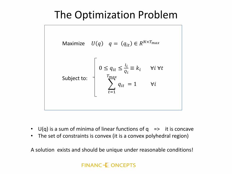
Conclusions

• Liquidity Modeling is an integral part of risk management. • In CCPs, liquidity is essential for constructing a sound margin system for portfolios. • Models should include portfolio size and time-horizon (model the close-out!) • CORE (BMF&F Bovespa) suggests constructing liquidity thresholds for each security and finding a liquidation strategy so that the worst value of the portfolio along the liquidation period under stress scenarios is optimized • In OTC markets, where prices are contributed by participants, liquidity polls for reference portfolios at different trade sizes can be used to build liquidity curves. • There is some indication that poll-based estimates are consistent with the CORE approach. Empirically we found that LCCs from polls are convex functions of trade size and appear to follow the ``1.5 model’’.