Recent advances in optimized geophysical survey … advances in optimized geophysical survey design ... Appropriate survey design is therefore critical to justify the ... applicable

R

H

le

©

G1

EOPHYSICS, VOL. 75, NO. 5 SEPTEMBER-OCTOBER 2010; P. 75A177–75A194, 13 FIGS., 1 TABLE.0.1190/1.3484194

ecent advances in optimized geophysical survey design

ansruedi Maurer1, Andrew Curtis2, and David E. Boerner3

fmlvTwHtpp

digocAtr

sstmmicohop

itatt

eived 1

rgh, U. K.gc.ca.

ABSTRACT

Survey design ultimately dictates the quality of subsurfaceinformation provided by practical implementations of geo-physical methods. It is therefore critical to design experimen-tal procedures that cost effectively produce those data thatmaximize the desired information. This review cites recentadvances in statistical experimental design techniques ap-plied in the earth sciences. Examples from geoelectrical,crosswell and surface seismic, and microseismic monitoringmethods are included. Using overdetermined 1D and 2D geo-electrical examples, a minor subset of judiciously chosenmeasurements provides a large percentage of the informationcontent theoretically offered by the geoelectrical method. Incontrast, an underdetermined 2D seismic traveltime tomog-raphy design study indicates that the information content in-creases almost linearly with the amount of traveltime datasource-receiver pairs considered until the underdetermi-nancy is reduced substantially.An experimental design studyof frequency-domain seismic-waveform inversion experi-ments reveals that a few optimally chosen frequencies offeras much subsurface information as the full bandwidth.Anon-linear experimental design for a seismic amplitude-versus-angle survey identifies those incidence angles most impor-tant for characterizing a reservoir. A nonlinear design exam-ple shows that designing microseismic monitoring surveysbased on array aperture is a poor strategy that almost certain-ly leads to suboptimal designs.

INTRODUCTION ANDHISTORICAL BACKGROUND

Geophysical surveys estimate specific aspects of the earth’s geo-ogical structure and composition. Such problems usually reduce tostimating the distribution of petrophysical properties of the subsur-

Manuscript received by the Editor 25 January 2010; revised manuscript rec1ETH Zürich, Zürich, Switzerland. E-mail: [email protected] of Edinburgh, School of GeoSciences, Grant Institute, Edinbu3Geological Survey of Canada, Ottawa, Canada. E-mail: dboerner@nrcan2010 Society of Exploration Geophysicists.All rights reserved.

75A177

Downloaded 15 Sep 2010 to 129.215.6.61. Redistribution subject to S

ace from measured data. To facilitate geological interpretation, nu-erous standardized data-acquisition procedures have been estab-

ished, and data processing and inversion algorithms have been de-eloped to extract estimates of the desired subsurface parameters.he importance of new processing, analysis, and inversion tools isidely appreciated and is the subject of considerable research effort.owever, it seems that much less attention has been paid to honing

he design of data-acquisition procedures the survey design. Thisaper focuses on ways to maximize the information content of geo-hysical-survey data sets.

An acceptable survey design should ensure acquisition of thoseata that best resolve specific subsurface features or parameters ofnterest Maurer and Boerner, 1998b; Curtis and Maurer, 2000. Thisoal is important because no amount of subsequent data processingr analysis can ever compensate for inadequate or missing data thatould have contributed significantly to resolving geological targets.ppropriate survey design is therefore critical to justify the cost of

he experiment in terms of the robustness, accuracy, and precision ofecovered geological information.

Philosophically, we desire an optimal data set that best resolvespecific subsurface petrophysical properties of the subsurface modele.g., composition, locations of discontinuities, porosity, and fluidaturation over a wide or a more focused subsurface volume fromhe acquired data. Yet in practice in most geophysical experiments,

odel parameters are nonlinearly related to the observable data,aking it extremely computationally demanding to calculate result-

ng constraints on parameter values. Also, the inverse problem ofonstraining model-parameter estimates from data observations isften ill posed no solution exactly satisfies the data and may notave a unique solution. Hence, the process of deciding which data tobserve to optimally constrain the interpretation of petrophysicalarameters is not straightforward.

One simple, often-used approach to the problem of insufficient ornadequate data is to acquire as much data as possible, including po-entially redundant data. However, cost is often a major consider-tion in geophysical surveying, implying that we need to find meanso acquire optimal data in terms of information content while main-aining a favorable cost/benefit ratio. Many geophysical-survey de-

1 May 2010; published online 14 September 2010.

. E-mail: [email protected].

EG license or copyright; see Terms of Use at http://segdl.org/

sgtvasi

mowsastpgscfi

aimnwtWevgooapr

etgqea

trtbaNtcd

ssTatvfecsl

cvetrewppao

cJpymso

wRoipfi

maaswadad

FSp

75A178 Maurer et al.

igns used in the past have been heuristic in the sense that they wereenerated from a combination of highly simplified theoretical inves-igations, repeated simulations with numerical or analog models ofery simple geological situations e.g., a perfectly stratified earth,nd experience gained from actual field surveys. Often, standard de-igns have been applied solely because they were required to use ex-sting analysis and inversion tools.

Although these approaches have been extremely successful inany cases, application of heuristic survey designs can be of dubi-

us value in dealing with logistical or instrumentation constraints, orith complex subsurface environments. Moreover, most survey de-

igns were constructed to obtain a complete image of the subsurface,nd they may not be appropriate for surveys conducted to resolvepecific types or subsets of subsurface petrophysical properties e.g.,hose from a specific depth interval of interest. With the current ca-ability for simulating the geophysical response of highly complexeological models and almost arbitrary survey designs, it wouldeem appropriate to explore whether better subsurface informationan be obtained from nonstandard approaches to experimental con-gurations.Qualitatively, the benefit of a geophysical survey can be defined

s the resulting net increase in resolution of the model parameters ofnterest. For example, an expected outcome of a geophysical survey

ight be to determine only the depth to a particular interface. Alter-atively, one may wish to resolve all physical-property variationsithin a restricted 3D volume. The extent to which these expecta-

ions are realized will dictate the success or failure of the experiment.ithin this seemingly broad spectrum of possibilities lies a common

lement: the reliability of the parameter information obtained by in-erting the geophysical data. We define the quantitative benefit of aeophysical experiment to be directly proportional to the resolutionr accuracy of the parameters necessary to answer specific questionsf interest. Resolution and accuracy can be estimated formally viapplication of linear or nonlinear inverse theory, so conceptually it isossible to find desirable survey layouts with optimization algo-ithms.

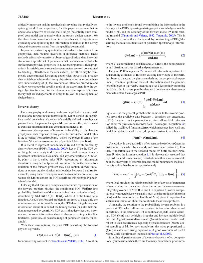
Figure 1 illustrates our notion of the relationship between the ben-fits and costs of performing a geophysical experiment. Althoughhis graph is qualitative, we expect the behavior of the limits to beenerally correct. For example, there is no benefit before data are ac-uired, although fixed costs are certainly incurred in mobilizingquipment and preparing for data acquisition. Additionally, benefitsre likely to be subject to the concept of diminishing returns such

Total experimental costs

Fixedcosts Variable costs

Sur

vey

bene

fits

Leve

loff

ull-c

oste

xper

imen

t

Maximum benefit achievable

igure 1. Schematic representation of cost/benefit relationships.hading is area of diminishing returns. Dotted line is optimized ex-erimental design. Solid line is standard experimental design.


hat ever-increasing data acquisition is likely to result in increasinglyedundant data rather than continually accruing benefits.Aside fromhe behavior at the limits of zero and infinite data, the details of cost/enefit curves are difficult to predict, primarily because of the gener-lly nonlinear relationship between data and model parameters.onlinearity effectively means that the values of the model parame-

ers influence the information content, and this makes it difficult toharacterize, a priori, the information content of specific observedata.

To understand Figure 1 more fully, consider a seismic crossholeurvey. In this case, the solid line might represent those designs con-isting of increasing numbers of evenly spaced shots and receivers.he variable cost for such designs will be approximately proportion-l to the amount of data collected and hence inversely proportional tohe shot and receiver spacing. On the other hand, one might find sur-ey designs that maximize cost savings for a given level of subsur-ace feature resolution or that maximize the benefit achievable atach given cost. Each of these objectives would result in a uniqueost/benefit curve where the cost/benefit ratio has been optimizeduch that the curve is shifted to a higher benefit level for any particu-ar survey expenditure dashed curve in Figure 1.

In reality, there is no single 2D graph equivalent to Figure 1 be-ause multiple dimensions of data-acquisition parameters could bearied for any given geophysical experiment, each defining a differ-nt cost/benefit function. Constructing optimized cost/benefit func-ions for multidimensional formulations is thus founded on the theo-y of statistical experimental design SED. For a geophysics-relat-d tutorial on SED, see Curtis 2004a, 2004b. SED techniquesere originally developed for optimizing industrial manufacturingrocesses. Cox 1958 formulated some of the first ideas about ex-erimental design, and Fedorov 1972 is credited with the first ex-mple of optimal experimental design by Atkinson and Donev1992, who also document much of the history of important devel-pments in industrial systems.

G. Taguchi developed and implemented design methods oftenalled Taguchi methods Taguchi, 1987 across a broad spectrum ofapanese industrial processes such that final products are as robust asossible to variations in the manufacturing steps. Over only a fewears, this led to a revolutionary increase in the quality of Japaneseanufacturing. Although Taguchi’s methods were often simple, he

ystematized an approach to quality control that did not exist previ-usly. Their simplicity makes these methods so generally applicable.

The first attempts at optimized experimental design in geophysicsere devoted to earthquake-location problems Kijko, 1977;abinowitz and Steinberg, 1990; Hardt and Scherbaum, 1994,cean tomography Barth and Wunsch, 1990, geoelectrical sound-ngs Glenn and Ward, 1976, and magnetotelluric investigationsJones and Foster, 1986. Building on ideas presented in these earlyapers, statistical experimental design has been continuously re-ned.Originally, statistical experimental design was treated as an opti-ization problem that could be solved with global optimizers such

s genetic algorithms e.g., Hardt and Scherbaum, 1994, simulatednnealing e.g., Barth and Wunsch, 1990, or multilevel coordinateearch e.g., Ajo-Franklin, 2009. Unfortunately, global optimizersere not yet efficient for larger-scale problems. Therefore, Curtis et

l. 2004 introduced a sequential approach that begins with severalesign parameters e.g., each describing a datum to be recorded thatre reduced in a stepwise fashion by removing the most redundantatum at each step. This algorithm is effective in designing simple


tmsgStmpw

smrstmwmepsitdtvg2soaopea

imiIsflttof

tslotjs

fmm

ghtot

oraoa

Optimized geophysical survey design 75A179

omographic surveys and micro-seismic monitoring surveys withany design parameters. Curtis and Wood 2004 showed that the

ame algorithm can be used to design optimal interrogation strate-ies to obtain geological information from human experts, andtummer et al. 2004 introduced sequential algorithms that work in

he opposite direction, beginning from a minimal design and incre-enting it with the most informative datum at each step; they ap-

lied this to design geoelectric experiments. Similar approachesere presented by Wilkinson et al. 2006 and Coles and Morgan

2009.To control computational requirements, many experimental de-

ign studies approximate nonlinear relationships between earth-odel parameters and the observed data with linear functions. The

ationale is that any inherent nonlinearity in the physical system is ofecond-order importance for small perturbations of model parame-ers. Although in many cases this approximation

ay be valid, a more rigorous and robust frame-ork for tackling concurrent or sequential experi-ental design optimization is offered by nonlin-

ar design methods. Algorithms for nonlinearroblems are generally computationally expen-ive and thus have been restricted to fairly specif-c problems that can be parameterized with rela-ively few 10 parameters. Examples includeesigning surface seismic receiver density or da-a-processing strategies for optimal amplitudeariation with offset/amplitude variation with an-le AVO/AVA analysis van den Berg et al.,003, 2005; Guest and Curtis 2009, 2010 or de-igning optimal receiver locations for earthquaker microseismic monitoring surveys Winterforsnd Curtis, 2008. Hyperparameterization meth-ds, recently applied in linearized geophysicalroblems Ajo-Franklin, 2009, are being extend-d successfully to fully nonlinear design methodspplicable for full 2D or 3D seismic surveysGuest and Curtis, 2010.

With the increasing success of statistical exper-mental design for geophysical applications, nu-

erous methodological studies and applicationmprovements have been published see Table 1.n this contribution, we first review the theory oftatistical experimental design. Then we show aew examples that demonstrate the benefits andimits of applying experimental design conceptso geophysical problems. In the concluding sec-ion, we critically review the achievements madever the past decade and outline potentially fruit-ul avenues of future research.

THEORY

The most important requirement in selectinghe experimental parameters for a geophysicalurvey design is to be clear in specifying the geo-ogical and operational objectives. Geologicalbjectives may range from being specific locatehe oil/water contact close to a planned well tra-ectory to vague create an image of some sub-urface volume to identify and locate anomalous

Table 1. Catstudies and ageophysical a

Application

Seismic tomo

Seismic reflec

AVO/AVA/AVprocessing str

Earthquake olocation surve

Electric or el

Other method


eatures that may be of interest. Operational objectives can often beore precisely defined and generally are based on the desire to mini-ize or control survey costs and the risk of operational failure.Once fully declared, all survey objectives are encoded into a sin-

le mathematical objective function that is intentionally chosen toave a minimum when a survey design best meets the desired objec-ives. Selecting the optimal survey design can then be achieved withne of several numerical minimization algorithms that vary parame-ers controlling the design until the minimum is attained.

Of the two components of the objective function, the operationalbjectives are not easily amenable to generic analysis because theyeflect a variety of highly specific influences, including price fluctu-tions, the specific survey equipment used, contractor experience,verhead costs, geographic location, and even weather conditionsnd season. Although accommodating operational objectives is a

s and representative published works of methodologicaltion improvements of statistical experimental design fortions.

Representative published work

Ajo-Franklin, 2009

Brenders and Pratt, 2007

Curtis and Snieder, 1997

Curtis, 1999a, 1999b

Maurer et al., 2009

Sirgue and Pratt, 2004

rveys Liner et al., 1999

rveys or Coles and Curtis, 2010

Guest and Curtis, 2009, 2010

van den Berg et al., 2003

seismic Curtis et al., 2004

Hardt and Scherbaum, 1994

Lomax et al., 2009

Rabinowitz and Steinberg, 1990

Steinberg et al., 1995

Winterfors and Curtis, 2008, 2010

agnetic surveys Coles and Morgan, 2009

Coscia et al., 2008

Furman et al., 2007

Hennig et al., 2008

Loke and Wilkinson, 2009

Maurer and Boerner, 1998a

Maurer et al., 2000

Oldenborger and Routh, 2009

Stummer et al., 2002, 2004

Wilkinson et al., 2006

al advances Curtis and Wood, 2004

Haber et al., 2008

Routh et al., 2005

egoriepplicapplica

graphy

tion su

Az suategies

r microys

ectrom

ologic


cqopted

gmssebpdsstd

I

bfpt

gif

dsrlamtewt

tpdfmitmfia

p

f

tdmiast

wo

ctittm

Eltcm

dttbh

wvIt

s

puimrlQM

t


ritically important task in geophysical surveying that typically re-uires great skill and experience, for this paper we assume that anperational objective exists and that a single potentially quite com-lex cost model can be used within the survey-design context. Weherefore focus on methods to achieve the other set of objectives —valuating and optimizing the information contained in the surveyata, subject to constraints from the specified cost model.

In practice, extracting quantitative subsurface information fromeophysical data requires inversion or inference methods. Theseethods effectively transform observed geophysical data into con-

traints on a specific set of parameters that describe a model of sub-urface petrophysical properties e.g., reservoir porosity, fluid prop-rties. Invariably, some subsurface parameters are well constrainedy data e.g., often those in the near surface, but others may be com-letely unconstrained. Designing geophysical surveys that produceata which best achieve the survey objectives requires a comprehen-ive understanding of 1 the inversion or inference procedure and2 how we encode the specific goals of the experiment into the de-ign objective function. We therefore now review aspects of inverseheory that are indispensable in order to follow the development ofesign theory.

nverse theory

Once any geophysical survey has been completed, a data set d wille available for geological interpretation. Let m denote the subsur-ace model consisting of a vector of spatially defined petrophysicalarameters in the parameter space M. Inversion is the process usedo translate information in d to constrain estimates of m.

An essential component of inversion is the ability to calculate theeophysical data response of any particular subsurface model. Thiss the so-called “forward problem,” which we express in terms of theunction f that relates m to a vector of predicted data: d f(m).

It is useful to represent uncertainty in m and d with probabilityensity functions PDFs; Tarantola, 2005. Let pd be the PDF de-cribing the uncertainty in d from all uncorrected measurement er-ors from instrumental bias, noise, and any other artifacts. Similar-y, pm is the so-called prior PDF, representing all informationbout m existing before prior to inversion. The mathematical for-ulation of the forward problem may also contain known limita-

ions in expressing the physical relationships between d and m, forxample, using linearized approximations to nonlinear relations; soe use d,m to denote the PDF describing this potentially uncer-

ain relationship.Let’s say that if fm is a complete and accurate representation of

he forward problem physics, the conditional PDF d m therobability distribution of d when m is fixed at a particular value isescribed by d m d fm, where is the Dirac deltaunction. Also, if the forward problem is assumed to place only theinimum constraints possible on m, the PDF describing this state of

nformation about m is called the homogeneous or null distribu-ion, represented by m. No PDF exists that describes zero infor-ation, but some information about m always exists in practice theniteness, positivity, or possible range of parameter values, for ex-mple.

With these assumptions, the joint PDF describing the forwardhysics is given by

d,mk d fmm 1

or normalizing constant k Tarantola and Valette, 1982.Asolution


o the inverse problem is found by combining the information in theata pd, the PDF expressing existing or prior knowledge about theodel pm, and the accuracy of the forward model d,m relat-

ng m and d Tarantola and Valette, 1982; Tarantola, 2005. This ischieved in a probabilistic framework by constructing a PDF Q de-cribing the total resultant state of posteriori postsurvey informa-ion:

Qd,mkpdd,mpm

d,m, 2

here k is a normalizing constant and d,m is the homogeneousr null distribution over data d and parameters m.

The joint PDF in equation 2 contains all information pertinent toonstraining estimates of m from existing knowledge of the earth,he observed data, and the physics underlying the geophysical exper-ment. The final, posteriori state of information about the parame-ers of interest m is given by integrating over d essentially summinghe PDFs of m for every possible data set d consistent with measure-

ents to obtain the marginal PDF:

QmkpmD

pdd,md,m

dd . 3

quation 3 is the general, probabilistic solution to the inverse prob-em from the available data because it describes the uncertaintyPDF characterizing the parameters m, given all available informa-ion about the physics and recorded data. The integral in equation 3 isalled the likelihood function Lm, which measures how well anyodel m explains data d. Hence, dropping constant k, we obtain

Qm pmLm . 4

Uncertainty in the data pd is often assumed to follow a Gaussianistribution, described by mean d0 and covariance matrix Cd. Fur-her, if uncertainties in the forward model d,m are negligible,hen takes the form in equation 1. It is also usually assumed thatd,m is a uniform constant distribution within some reasonableounds. In a system of discrete data and model parameters, the likeli-ood function then becomes approximately

Lmexp1

2d0 fmTCd

1d0 fm, 5

here Lx provides the relative probability of any set of parameteralues m being the true values, given the current data measurements.ntegrating over all of MD to find k in equation 3 is often compu-ationally intractable, so we usually must use the product of the prior

pm and the nonnormalized likelihood Lm given in equation 4 asufficient information about the solution to the inverse problem.

Ultimately, the solution to the probabilistic inverse problem is aosteriori PDF, which allows one to extract information about m andncertainty in the estimation. If f is nonlinear or pd is non-Gauss-an, PDF Qm may be highly irregular and include multiple localaxima.Algorithms used to estimate Q must therefore then be made

obust to such occurrences, typically by pseudorandom Monte Car-o sampling of M. For each sample mi, the value proportional tomi is calculated using equation 4. A good overview of usefulonte Carlo algorithms is included in Press et al. 2007.Sampling all pertinent parts of the model space is often computa-

ionally unfeasible when there are too many parameters, prior infor-


mmIQpwaIcbma

L

ssdumta

i

wiwmwlt

pbet

ITp

lttps

wmst

cafrvpaie

ma

ittti

Ozo

ctvriDm

ttmsurpt

D

temtf

specc


ation with which to constrain the range of model-parameter esti-ates is too limited, or the forward relation in is highly nonlinear.

n such cases, it is usual to approximate the posteriori distributionm to create a tractable inverse problem solution, usually by ap-roximating fm with a linear function. However, when the for-ard relationship f is truly nonlinear, iterative application of linear

pproximations complicates the interpretation of inversion results.naccuracies in the linear approximations cannot be observed in theomputational results from the linearized model alone and will onlye apparent from comparisons with nonlinear models. Nevertheless,any geophysical problems are currently intractable without linear

pproximations and hence are often used.

inearized approximations

Linear approximations are covered in many excellent texts andummary papers e.g., Matsu’ura and Hirata, 1982; Menke, 1984,o we only describe key concepts that are relevant for experimentalesign. A linear approximation is derived for model-parameter val-es in the region around some reference model m0. This referenceodel is usually the mean or the maximum-likelihood model from

he prior model PDF. If the derivatives of f evaluated at any model mre denoted by the matrix F, where the ijth element is

Fijm f i

mjm, 6

nitially where mm0, then the linearized approximation to f is

dd0Fmm0Omm02, 7

here d0 fm0. The higher-order terms Omm02 are ignoredn the linear approximation and thus represent the error associatedith the linear assumption. Once ignored in the mathematical for-ulation, any errors associated with these terms will not be apparentithout additional calculations using nonlinear models. Neverthe-

ess, this approximation is usually valid in some vicinity of m0; fromhis point on in this subsection, we ignore these higher-order terms.

Because the reference model m0 is known, the linearized inverseroblem reduces to estimating the vector of model parameter pertur-ations mestmm0. A corresponding inverse operator F1 thatstimates the model parameters by minimizing the discrepancy be-ween d and d0 can be written as

mestF1dd0 . 8

n geophysical problems, F is generally singular or nearly singular.his is the result of inherent ambiguities and/or insufficient and im-recise data. Hence, F1 must be approximated.

There are several options for approximating F1, the most popu-ar being to include regularization constraints that reduce the effec-ive number of degrees of freedom by enforcing desired behavior onhe model parameters e.g., see Matsu’ura and Hirata, 1982. In thisaper, we consider the commonly used iterative Gauss-Newtoncheme:

mi1est FTCD

1FCM11FTdd0Fmi

est,

9

here i is the iteration number m0est is set to the initial reference

odel m0; CD is the data covariance matrix that describes all mea-urement uncertainties of d; CM is the a priori model covariance ma-rix, which allows regularization constraints, such as requiring spe-


ific spatial variations e.g., smoothness, roughness, minimum vari-tion from the reference model in model parameter values to be en-orced. Importantly, regularization should be selected such that itepresents our prior expectations of the posteriori model-parameterariations. A least-squares l2-norm misfit objective function is im-licit in equation 9. To maintain assumptions behind the linearizedpproximation, the optimization procedure to estimate m is appliedteratively so that the sensitivities contained in F in equation 6 are re-valuated at the best estimate of the model-parameter vector m

miestmi1 at iteration i1.

The quality of the result of an inversion of a truly linear forwardodel can be appraised by examining the model resolution matrix R

nd the posteriori model parameter covariance matrix C, defined as

R FTCD1FCM

11FTCD1F, 10

C FTCD1FCM

11 11

e.g., Menke, 1984, where F in equations 10 and 11 is evaluated us-ng equation 6 with m set to the final estimate of parameters m fromhe iterative optimization procedure. The resolution matrix R relateshe final estimated model parameters mest to the true model-parame-er perturbations mt because, by substituting dd0 Fmtmt

estn equation 9,

mestRmt. 12

f particular interest are the diagonal elements of R: values close toero indicate poorly resolved model parameters, and values close tone indicate well-resolved model parameters.

The posteriori covariance matrix in equation 11 translates data un-ertainties CD into the space of model parameters and combineshem with the prior parameter uncertainties to estimate posteriori co-ariances. Off-diagonal elements indicate the degree to which pa-ameter estimates remain correlated postinversion i.e., large valuesndicate pairs of parameters that are not independently resolvable.iagonal elements are the variances of individual parameter esti-ates, and small values indicate well-resolved parameters.Finally, we again note that equations 10 and 11 are only valid for

ruly linear forward models. When the models contain nonlineari-ies, interpretation of the resolution offered by a data set requires a

ore sophisticated approach e.g., Stark, 2008, and experiencehows that estimates of linearized posteriori uncertainty in CD aresually severely underestimated. In such cases, the quality of poste-iori parameter estimates should be quantified by calculating or sam-ling the posteriori parameter PDF using equations 3–5 if computa-ionally possible.

esign theory

Geophysical survey design theory consists of methods to selecthe data-acquisition parameters such that model parameters of inter-st are resolved optimally. The same theory has been used to opti-ize the model parameterization to best represent information con-

ained in the data e.g., Curtis and Snieder, 1997. However, here weocus on the former mode of application.

The inverse problem solutions in equations 3 and 9 are con-trained by d, by the PDF of prior information on m, and by forward-roblem physics relating d and m. Survey-design methods influ-nce the form of this inverse problem and hence its solution byhanging which data should be recorded. The goal of the design pro-edure is to collect those data such that the pertinent information de-


sttp

fft

HcaPabodaat

atrQocdmscp

ptobldC2tpC2

dasod

I

S

c

exi

woksot

maiibe

Uittrbn

fastlomtotweltd

rubttbie

mso


cribed by solution Qm is maximized. The design problem isherefore a macro-optimization problem where, prior to the surveyaking place, we optimize design the inverse problem that we ex-ect to solve after the survey has occurred.

The selected design is the one that maximizes some objectiveunction. Ignoring cost and logistics for the moment, this objectiveunction is usually taken to be some measure of expected informa-ion:

J Emt IQm; ,mt . 13

ere, is a vector describing the design e.g., source and receiver lo-ations, shot fold, particular equipment to be used, IQm; ,mt ismeasure of the information contained in the resulting posterioriDF Qm for when the true model parameters are given by mt,nd the statistical expectation operator Emt

averages I over the distri-ution of all possible values for the true model mt, which by our pri-r knowledge is expected to be distributed according to the prioristribution pm. The value J should be maximized. If, instead,minimization problem is desired e.g., to combine with cost, whichlso should be minimized, then the negative of the measure in equa-ion 13 can be used.

Within the expectation in equation 13, the design criterion takesccount of all possible potential values mt, their prior PDF pm, andhe corresponding data including their uncertainties expected to beecorded for each model uncertainties are accounted for withinm. To calculate the expectation usually requires integrationver a far greater proportion of the model and data spaces M and Dompared to the solution of the inverse problem after a particularata set has been recorded where pd is fixed and limited by actualeasurements and hence Qm is generally more tightly con-

trained. Consequently, experimental design is usually far moreomputationally costly than solving any particular inverse problemostexperiment.

For this reason, design methods that capitalize on linearized ap-roximations to the model-data relationship m,d similar tohose described above that are used for inversion have by necessityften been used for designing surveys e.g., Rabinowitz and Stein-erg, 1990; Steinberg et al., 1995; see Curtis, 2004a. Nonprobabi-istic methods which do not explicitly consider the prior probabilityistribution have also been used e.g., Maurer and Boerner 1998a;urtis, 1999a, 1999b; Stummer et al., 2004; Coles and Morgan,009. Truly nonlinearized design methods that optimize the objec-ive function in equation 13 have been developed in geophysicalroblems only relatively recently van den Berg et al., 2003, 2005;urtis, 2004b; Winterfors and Curtis, 2008; Guest and Curtis, 2009,010.

The key to understanding any particular design method is to un-erstand 1 whether the physics describing the forward model arepproximated e.g., linearized or whether the full physics are con-idered, 2 which information measure I is used in equation 13, and3 how the macro-optimization is achieved. In recent years, devel-pments have occurred in all three areas within geophysical survey-esign applications.

nformation measures and (non)linear physics

hannon information

A critical concept in information theory is that the informationontent of an uncertain noisy process is determined by the process


ntropy Shannon, 1948. If X is a random variable that takes a valuewhich varies probabilistically with PDF px, then the Shannon

nformation IShan is defined by

IShanpxcentXx

pxlogpxdx,

14

here c is a constant. The entropy entX is a measure in the sensef an expected value of the information in the PDF px. In his well-nown paper of 1948, Shannon shows that entropy is the only mea-ure with a certain set of desirable properties e.g., linear additivityf the information associated with independent pieces of informa-ion.

By setting I IShan in equation 13, the design process will maxi-ize an objective function that measures the expected amount of Sh-

nnon information in the posteriori probability distribution Qm,.e., in the PDF of m after the survey has taken place. The constant cn equation 14 is irrelevant and can be set to zero for design purposesecause maximizing IShan for c0 will also maximize it for any oth-r value of c.

The main limitation with this design approach is computational.nless the PDF is nonzero over a finite range, numerically evaluat-

ng the entropy to approximate the integral in equation 14 is compu-ationally intensive. In addition, for values of x with small probabili-ies px, logpx is very large and negative, and it often variesapidly with px, meaning many samples are needed to obtain a ro-ust approximation of the integral to estimate the entropy or Shan-on information.

Although setting I IShan in equation 13 requires substantial ef-ort to sample each Qm adequately, in nonlinear problems the situ-tion is even worse. By examining equation 3, it is apparent thatampling Qm is equivalent to solving an inverse problem. Whenhe forward physical relationship deviates significantly from beinginear, inversion is performed using full Monte Carlo inverse meth-ds or it proceeds iteratively by solving a sequence of linearizedodels using equations such as equation 9; either process can be ex-

remely demanding computationally. Furthermore, the expectationperator in equation 13 requires us to evaluate the Shannon informa-ion for the full range of posteriori PDF distributions of Qm thate are likely to encounter postsurvey i.e., we would need to invert

very possible data set that might be recorded in the experiment, or ateast a representative selection of them. Without additional insight,his approach could only be implemented for simple experimentalesign problems e.g., one or two model parameters and data.

The computational limitations inherent in this formulation can beeduced significantly by Shewry and Wynn’s 1987 breakthrough:nder certain conditions, the Shannon information can be obtainedy maximizing the entropy in the data space entpd rather than inhe model space entQm. Shewry and Wynn’s conditions requirehat pm and the data uncertainties, on each individual datum in de independent of the survey design see Curtis 2004b for a tutorialllustrating this conceptual step. Computing entpd requires anstimate of the PDF pd, which can be calculated by projecting

pm into data space through the forward model by taking samplesi of m according to pm and calculating di fmi. The resulting

et di will be distributed according to pd. Evaluating entpdnly requires evaluating f rather than solving the inverse problem.


etfpcmi

psnDitnfdAHwdp

M

v

wsvpr

ntvmh

ptlBatemgcti

apm

cctauwce“dlWlfii

tadbtasotds

T2sm

tdtdws

otwdb

T

Tn


Even with the simplifications afforded by the assumptions of Sh-wry and Wynn 1987, the computational challenge of experimen-al design that maximizes Shannon information remains significantor many geophysical problems. However, if implemented with ap-ropriate Monte Carlo and optimization algorithms, these methodsan be computationally tractable for several important geophysicalethods, including designing surface seismic surveys and optimiz-

ng data-processing strategies e.g., Guest and Curtis, 2009, 2010.For linear problems, maximizing Shannon information is not de-

endent on the true model see Curtis, 2004a; hence, it is unneces-ary to calculate the expectation in equation 13. Maximizing Shan-on information is then also equivalent to maximizing the so-called-criterion different design criteria are assigned different alphabet-

cal names; see Atkinson and Donev 1992 for an overview. In sta-istical literature the D-criterion is usually defined to be the determi-ant detFTF; but as in equation 11, it can be extended to take theorm detFTCD

1F to incorporate data uncertainties, or toetFTCD

1FCM1 to include the effects of model regularization.

lternatively, using a nonprobabilistic approach, Matsu’ura andirata 1982 provide a formalism that allows F to be consistentlyeighted such that detFTF accounts for variations in confidence inifferent data or for focusing the information measure on differentarameters of particular interest.

easures of variance

Variance is defined as the expected squared deviation of a randomariable, say, X, about its mean:

VXX

EXEX2dX, 15

hich measures the expected degree of variation of X. We often de-ire solutions to geophysical problems that have minimum possibleariance on the model parameters because such solutions will be ex-ected to be constrained around some limited range of the model pa-ameter space M.

A principal limitation in using Shannon information to designonlinear problems is that it does not necessarily discriminate be-ween designs that result in high or low variance in the expected in-ersion solution. Optimal designs might therefore generate maxi-um Shannon information in the inverse problem solution yet retain

igh variance in that solution.To understand this counterintuitive statement, consider a PDF

1x that allows x to have only one of two distinct values, one orhree, each with equal probability, and a second PDF p2x that al-ows x to have only the values zero and four with equal probability.oth PDFs contain identical Shannon information because they bothllow only two possible values for x; hence, in this sense, x is equallyightly constrained by either PDF: IShanp1x IShanp2x. How-ver, solution p2x has a higher variance than p1x around the com-on mean value of two. We would usually prefer a design that would

ive postsurvey solution p1x over one that would give p2x be-ause the latter more tightly constrains the range of values of x, evenhough the number of possible values that x can assume is the samen each case.

For this reason, in nonlinear problems, it is often desirable to cre-te designs that will minimize some measure of spread, such as ex-ected variance IV in equation 13, rather than designs that onlyaximize Shannon information I I . There is also a distinct
Shan

omputational advantage in avoiding the calculation of an integrandontaining a logarithm as in equation 14, as explained above. Hence,he design problem is generally numerically more tractable for vari-nce than for Shannon information. Nevertheless, we confront thesual numerical challenge known as the curse of dimensionality,hich states that computational effort required for integration in-

reases geometrically as the dimensionality of the integrand increas-s Curtis and Lomax, 2001. Hence, it is necessary to look forsmart” methods to approximate the variance or to define less-bur-ensome measures of spread that are efficient for nonlinear prob-ems. In the following, we explain one useful alternative derived by

interfors and Curtis personal communication, 2010 that is ana-ytically related to variance and is so sufficiently computationally ef-cient that it has been used to design multisensor microseismic mon-

toring surveys.Variance or spread is fundamentally related to the distance be-

ween different parameter values points in model space M that arembiguous with respect to i.e., are not discriminated by recordedata. Given two points mm in M the dots are indices, it is possi-le to create various measures of how likely these are to give rise tohe same observation — and hence be indistinguishable given suchn observation. This is determined by the extent to which their re-pective data-space probability densities pd m, and pd m, verlap, where is a vector that defines the survey design. These dis-ributions each describe the probability of recording any data vectorif the true parameter values were represented by model m or m, re-

pectively. The most straightforward option for such a measure is

Sm,m, d

pdm, pdm, dD . 16

his defines a so-called bifocal measure Winterfors and Curtis,008, simultaneously focusing on two points m,m in parameterpace instead of only one, which is the most common approach e.g.,easure IShan in equation 14.The measure in equation 16 does, however, have two disadvan-

ages: 1 Sm,m, is always high for mm, even though this caseoes not contribute to uncertainty in estimates of the model parame-ers m, and 2 the unit of Sm,m, is the same as of a probabilityensity pd over data space, implying that Sm,m, will increaseith decreased observational uncertainty the opposite ideally

hould be the case for a useful measure of parameter uncertainty.Winterfors and Curtis personal communication, 2010 show that

ne way to overcome the first problem is to multiply Sm,m, byhe squared distance between m and m assuming that D is equippedith a distance metric d. The second problem can be addressed byividing Sm,m, by a measure TD of average observational proba-ility density:

TD dD

pd pd dD . 17

his results in the ambiguity measure:

Rm,m, d2m,m

TDSm,m, . 18

o create a global measure of the ambiguity of an investigation tech-ique design, it is necessary to take the expectation of Rm,m,


ot

Tasca

sa

wtPCeb

getalwWvssws

osieVt

tvestAt

O

Dmoaoa

wCs

uvomwisatst

malamctlwsci

Ftmtuet


ver all possible point pairs in model parameter space, with respecto the prior parameter PDF pm:

W mM

mM

pmpmRm,m, dMdM . 19

he expected observational ambiguity W is thus a measure of theverage ambiguity of all possible observations, given a survey de-ign and a prior distribution over parameter values. Therefore, W an be used to evaluate or design surveys described by prior to thecquisition of any observations.

Furthermore, W relates to the expected posteriori variance in aimple manner: inserting equation 17 into 18, applying Bayes’ rule,nd changing the order of integration gives

W 2

TD

dD

p2d Vmd, dD, 20

here, if the distance metric d is the standard Euclidian distance,hen Vm d, is equal to the variance of the posteriori model spaceDF, given the data d from a survey with design Winterfors andurtis, personal communication, 2010. Thus, W , as defined inquation 19, is the expected variance of the posteriori PDF, weightedy pd .

The advantage offered by optimizing using this measure of ambi-uity rather than the variance itself is that to calculate W usingquations 16–19 requires only forward-model calculations calcula-ions of the PDF of d given m on the right-hand side of equations 16nd 17. Calculation of the variance V in equation 20 requires calcu-ating the expected variance of the posteriori PDF of m given d,hich requires the inverse problem solution. Similar to Shewry andynn 1987, this approximation obviates the need to solve the in-

erse problem, helping to reduce the effect of the curse of dimen-ionality. Winterfors and Curtis personal communication, 2010how that using W is particularly computationally advantageoushen data uncertainties can be represented by closed-form PDFs

uch as Gaussian, Poisson, or Laplacian distribution functions.

Normalized eigenvalue index

Nor

mal

ized

eige

nval

ues

0 1

100

Threshold

Spectrum1

Spectrum2

RER1

RER2

Null space1

Null space2

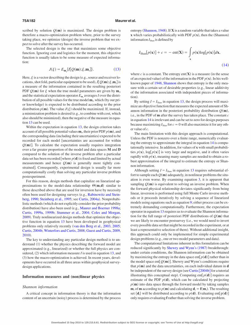
igure 2. Representation of two normalized eigenvalue spectra ofhe Hessian matrix FTCD

1F equation 9. The horizontal axis is nor-alized with respect to the total number of model parameters, and

he vertical axis is normalized with respect to the largest eigenval-es. Dashed line indicates the threshold level that defines the relativeigenvalue range RER. RER1,2 indicate measures of quality of the
wo surveys.

Minimizing W does not seem to fit into the general frameworkf equation 13 because the integration is over the data space D in-tead of the model space M. To optimize with respect to the ambigu-ty measure, we have to replace J by W in equation 13. How-ver, as shown, W can be thought of as a reweighted alternative toover the model space, and V does fit into the framework of equa-

ion 13 by setting IV.In linear models with normally distributed uncertainties, the pos-

eriori variance Vm d, will be constant with respect to the obser-ation d. As a consequence, optimizing W will then be exactlyquivalent to optimizing the expected posteriori variance. In lineartatistical experimental design literature, optimizing designs suchhat their expected posteriori variance is minimized is known as the-optimality criterion. This corresponds to minimizing the sum of

he variances diagonal elements of C in equation 11.

ther information measures

In subsequent examples, we use two other measures related to the-criterion. Besides the determinant of the matrix FTCD

1F, oneay also consider its eigenvalue spectrum. For the perspective of

ptimizing the resolution of the complete suite of model parameters,n optimized design should result in a small condition number ratiof the largest to the smallest eigenvalue of FTCD

1F. This can bechieved by minimizing

i

1

i, 21

here i are the eigenvalues and is a small positive constant seeurtis 1999b for an extensive discussion of this and related mea-

ures.Another possible choice is to define a measure that is related to the

nresolved part of the model space null space. The choice of a sur-ey layout governs the structure of the matrix F, and close inspectionf equation 9 indicates that the reliability of the parameter estimates

est depends primarily on our ability to invert the matrix FTCD1F

CM1. Without the regularization constraints in CM

1, this matrixould likely be singular, such that its determinant would be zero and

ts condition number would be infinite. The sensitivities in F repre-ent the information content offered by a particular survey designnd CM

1 indicates our preconceived ideas on the subsurface struc-ure e.g., closeness to a prior model estimate or that it should havemooth spatial variations, so it is certainly advisable to maximizehe contribution of FTCD

1F and to minimize the influence of CM1.

Figure 2 shows two typical eigenvalue spectra of FTCD1F as they

ay arise from a geophysical inversion experiment. The verticalxis is logarithmically scaled and normalized with respect to theargest eigenvalue of the corresponding spectra, and the horizontalxis is normalized by the total number of eigenvalues number ofodel parameters. Because of the finite precision of numerical

omputations, eigenvalues are rarely identical to zero, even whenhe matrix is singular. Therefore, a threshold must be introduced be-ow wherein the eigenvalues are considered to be insignificantdashed line in Figure 2. The intersections of the eigenvalue spectraith the threshold line indicate the portions of the resolved model

pace and the unresolved null space. We define the range of signifi-ant eigenvalues, the relative eigenvalue range RER, to be the hor-zontal coordinate of the intersection point. This provides a simple


ads

M

fttgaMra2s

drsCasle

wwsamwrtttdl

barstcsttmotsr

E

medwfiT

mtf

Ftttii


nd intuitive means for quantifying the quality of a particular surveyesign. For example, the hypothetical survey design 2 in Figure 2 isuperior to survey design 1.

acro-optimization methods

Ideally, when designing an experiment, one searches exhaustivelyor the design that optimizes the design objective function in equa-ion 13. A variety of minimization algorithms are available for thisask. The most popular method historically has been the Detmax al-orithm Mitchell, 1974. However, other authors have used geneticlgorithms Hardt and Scherbaum, 1994; Curtis and Snieder, 1997;aurer and Boerner, 1998a; Curtis, 1999a, 1999b, simplex algo-

ithms Winterfors and Curtis, 2008, simulated annealing Barthnd Wunsch, 1990, or multilevel coordinate search Ajo-Franklin,009. Conceptually, any global optimizer can be used. The mostuitable choice is problem dependent.

When there are multiple design parameters, searching the entireesign space the space of all permissible combinations of design pa-ameters may be computationally unfeasible. Sequential designtrategies have been developed in many linear design studies e.g.,urtis et al., 2004; Stummer et al., 2004; Coles and Morgan, 2009,nd Guest and Curtis 2009, 2010 introduce a sequential designtrategy applicable to nonlinear problems. Such algorithms general-y increment the number of elements within the design vector forach iteration:

jarg maxJ j, such that j1 is fixed, 22

here j 1, . . . , j, with i an element of the design vector , andhere J is the objective function in equation 13. The new optimal de-

ign j combines the design defined at the previous iteration j1,ugmented by the single datum defined by j that maximizes mini-izes the objective function given that j1 remains fixed. In thisay, the work required to design an experiment with n design pa-

ameters is reduced from searching an n-dimensional design spaceo n separate searches of 1D design spaces. Although at each itera-ion the design is only locally optimal, Guest and Curtis 2009 showhat for nonlinear AVO/AVA design problems, the locally optimalesign is almost identical to the globally optimal design for prob-ems in which the globally optimal design could be calculated.

The choice of which specific algorithm to use should in principlee affected by the so-called no-free-lunch NFL theorems Wolpertnd Macready, 1997. These state that no single optimization algo-ithm is ideally suited for all objective functions and conversely, noingle objective function is ideally suited to be minimized by all op-imization algorithms. D. Coles and A. Curtis personal communi-ation, 2010 examine the influence of NFL theorems on linearizedtatistical experimental design by comparing several sequential op-imization algorithms on three quite different design objective func-ions. They show that within this limited context, a clear ranking is

ade between the optimization algorithms: almost regardless of thebjective function, the best algorithm allows incremental augmenta-ion and reduction of the design at each iteration. Hence, somewhaturprisingly, Coles and Curtis do not observe the effect of NFL theo-ems within this limited context.


EXAMPLES

xample 1: Designing geoelectrical experiments

Geoelectrical methods have been applied with great success forany years e.g., Butler 2005 and references therein. Until the

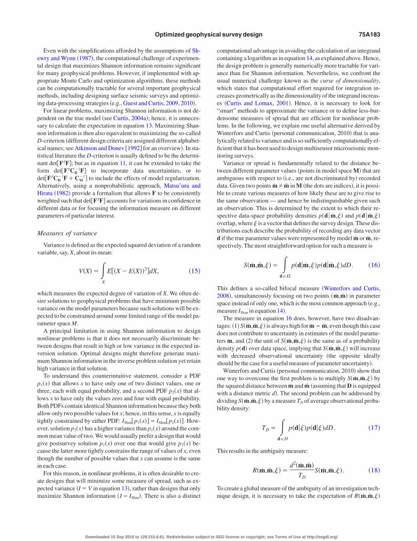
arly 1990s, interpretation of geoelectrical data was performed pre-ominantly in terms of layered-earth models, and the measurementsere conducted almost exclusively with standardized electrode con-gurations such as Schlumberger, Wenner, or dipole-dipole e.g.,elford et al., 1990.Figure 3a shows a Schlumberger electrode configuration. Theeasuring dipole is centered in the configuration, and the two elec-

rodes, where current is injected, are each deployed at a distance rrom the center. Schlumberger experimental design thus consists of

Subsurface

r r

Number of data points

Nor

mal

ized

desi

gngo

odne

ss 1.0

0.8

0.6

0.4

0.2

0.00 10 20 30 40

c)

Conductivity (S/m)

100

101

102

Dep

th(m

)

b)

–410 –210

Current injection electrode

Measuring dipole (length << r )

a)

igure 3. A 1D geoelectrical survey design. a Schematic represen-ation of a Schlumberger sounding. b Subsurface model used forhe experimental design. c Cost/benefit curves for a design wherehe current electrode separation is increased geometrically thin sol-d curve and optimized design thick solid curve. The dotted linendicates the normalized goodness of 1.0.


vasd

stml

lsbimt

gnba

safcsdttsic

a

c

e

g

Fevvtd


arying a single parameter, the distance r between the current sourcend sink. Traditionally, r is varied over a suite of regularly log-paced distances. The resulting data are then inverted for layer con-uctivities and layer thicknesses.

A typical layered-earth model with a conductive middle layer ishown in Figure 3b. Our goal is to constrain all five model parame-ers three layer conductivities and two layer thicknesses in an opti-

al fashion. The data space consists of 40 distances r, logarithmical-y spaced over a range of 1–10,000 m.

Intuitively, one might expect optimal layouts to include more-or-ess equally log-spaced recording distances, as suggested by the sen-itivity design studies of Oldenburg 1978. Figure 3c shows cost/enefit curves for equally log-spaced experiments sequentially add-ng larger r values to the design and optimally designed experi-

ents using a genetic algorithm see Maurer et al. 2000 for de-ails. The optimized experiment is found by maximizing the design-

Dep

th(m

)D

epth

(m)

Dep

th(m

)

Distance (m) Distan

0102030405060

0102030405060

0102030405060 0 20 40 60 80 100 120 140 0 20 40 60

282 data points

670 data points

) b)

) d)

) f)

0 1 2 3 4

Log10 resistivity (Ω m)

Distance (m)

0102030405060

Numbe

Rel

ativ

ere

solu

tion

(%)

100

80

60

40

20

0

0 20 40 60 80 100 120 140

0 2000

Dep

th(m

)

) h)

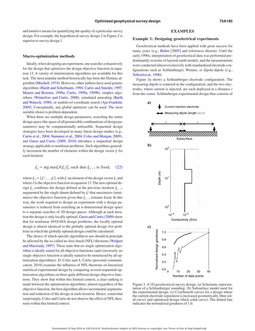
igure 4. A 2D geoelectrical survey design. a True subsurface molectrodes vertical arrows. b Inversion result using the comprehenersion results obtained with a combination of Wenner and dipole-dersion results with the optimized data sets. g Depth range filled bhe cost/benefit curve in h is constructed. The star in h denotes theata set, and the vertical arrows indicate the results for the optimized–f.


oodness measure in equation 21. Benefit is expressed as aormalized goodness goodness of a particular experiment dividedy goodness of the complete data set of 40 distances, and costs aressumed to be proportional to the number of measurements.

For the equally log-spaced design, the curve in Figure 3c exhibitsome erratic behavior. This indicates that rigidly incrementing r log-rithmically can provide data that contain only limited informationor resolving the five model parameters. The goodness can even de-rease when more data points are added by following a rigid log-pace sampling strategy. This is caused when particularly criticalistances might be missed using a rigid sampling scheme. In the op-imized design, the goodness increases monotonically and reacheshe level of the full-scale experiment at about 20 data points. The re-ult suggests that conventional Schlumberger DC resistivity sound-ngs might be made substantially more cost effective by a judicioushoice of r values needed to resolve the earth model. Maurer et al.

2000 also discuss strategies for optimized lay-outs suitable for a range of different subsurfacemodels.

The simple layered-earth experiment shown inFigure 3 is interesting conceptually but of limitedpractical relevance. Today, it is more commonthat geoelectrical data are acquired using multi-electrode systems e.g., Griffiths and Turnbull,1985; Stummer et al., 2002. Such data sets are in-verted tomographically e.g., Loke and Barker,1996 to create 2D and 3D subsurface images,which provide substantially more realistic infor-mation about the earth compared with layered-earth models. The data space of such experimentscan be very large. For an n-electrode array, thereexist nn1n2n3 /8 nonreciprocalconfigurations. For experiments using 30, 50, and100 electrodes, one conceptually could have82,215; 690,900; and 11,763,675 data measure-ments. These types of experiments are extremelydifficult to design because there are no heuristicmeans by which to determine the type and num-ber of configurations that would provide favor-able cost/benefit ratios.

Statistical experimental design, as applied tothe simple Schlumberger sounding example, iscomputationally too expensive for 2D or 3D earthmodels because the goodness function wouldhave to be evaluated many times during globaloptimization. Therefore, Stummer et al. 2004propose a sequential design strategy, whereby aninitial measurement configuration is chosen andthen sequentially augmented until the desiredbenefit level is reached. The initial data set can beone of the standard electrode configurations oreven a single set of injecting and measuring bi-poles. The choice of the next electrode configura-tion in the sequence is governed by examiningwhich has the largest potential of adding informa-tion content. Stummer et al. 2004 define an in-cremental information measure based on the lin-ear independence of a candidate configurationwith respect to the configurations already select-ed. Furthermore, they consider the relative in-

100 120 140

data points

data points

data points

ta points10000

d position ofata set. c In-ata. d–f In-ea for whichdipole-dipolesets shown in

ce (m)80

282

51373

1050

r of da6000

del ansive dipole dlack arinitiald data


ctsFat

oactrtsmFnftprd

tectqpmchupm

cuaspoodmapttc

ltuaidS

ds

E

T

gccsicebDonmttdb

a

a

b

Fpilhhshe


rease of the formal resolution defined via the model resolution ma-rix; see equation 10 within the individual model cells. There isome latitude on how to define the value of incremental information.or example, Wilkinson et al. 2006, Coscia et al. 2008, and Lokend Wilkinson 2009 use measures based entirely on the increase ofhe formal resolution.

The 2D example shown in Figure 4 is adapted from Stummer et al.2004. Figure 4a shows the true subsurface model and a deploymentf a 30-electrode array. From all possible configurations of injectionnd measuring dipoles, we exclude those with crossed injecting andurrent dipoles and configurations with unfavorable geometric fac-ors, leaving 51,337 out of a possible 82,215 measurement configu-ations. Stummer et al. 2004 denote this reduced suite of configura-ions as a comprehensive data set. Inversion of a comprehensive dataet leads to the image shown in Figure 4b. It reflects the total infor-ation content offered by the complete data space. For comparison,igure 4c shows the result using a combination of all possible Wen-er and dipole-dipole configurations subject to the same geometricactor restrictions as for the comprehensive data set: 282 configura-ions.At shallow depths, the tomograms in Figure 4b and c are com-arable, but other electrode configurations are apparently needed toesolve the deep conductive feature between x20 and 40 m and d

10 and 30 m that is recovered in the inversion of the completeata set.

Although Figure 4b and c demonstrates that traditional configura-ions do not recover the full information content offered by the geo-lectrical method, collecting a comprehensive data set would not beost effective. Determining the appropriate measurement configura-ions requires optimized experimental design. We follow the se-uential design strategy of Stummer et al. 2004 and start with a di-ole-dipole data set 147 data points; then we add successivelyore configurations. At 282 data points the same number as the

ombined Wenner/dipole-dipole data set, the information contentas already improved compare the inversion results shown in Fig-re 4c and d. Successively adding further data leads to dramatic im-rovements of the recovered images Figure 4e and f using only ainor fraction 2% of the complete data set.The image-quality increase can be quantified by analyzing the in-

rease of the formal resolution. For example, imagine we are partic-larly interested in resolving the depth range of the conductivenomaly. To quantify this, we sum the normalized resolution corre-ponding diagonal elements of the model resolution matrix ex-ressed as a percentage of the comprehensive data-set experimentf the cells highlighted in Figure 4g and plot the average relative res-lution as a function of the number of data points. The initial dipole-ipole data set provides only approximately 20% of the total infor-ation content in this depth range. When further configurations are

dded, the relative resolution increases quickly. At about 1000 dataoints, the cost/benefit curve enters into the realm of diminishing re-urns. In fact, the image in Figure 4f is already quite comparable tohose of the comprehensive data set, and it is very similar to imagesonstructed with 2000, 5000, and 10,000 data points not shown.

The sequential experimental design procedure Figure 4 is calcu-ated using sensitivities for a homogeneous half-space to representhe state of knowledge prior to an experiment. One might expect thatsing this approximation when the current-flow patterns and thuslso the sensitivities are disturbed by the presence of the conductiv-ty anomalies of the true model Figure 4a would lead to suboptimalesign results. Surprisingly, this is not the case, as demonstrated intummer et al. 2004. This also indicates that linear experimental


esign is adequate for such types of problems; the much more expen-ive nonlinear methods are not expected to provide superior results.

xample 2: Designing seismic crosshole experiments

raveltime tomography

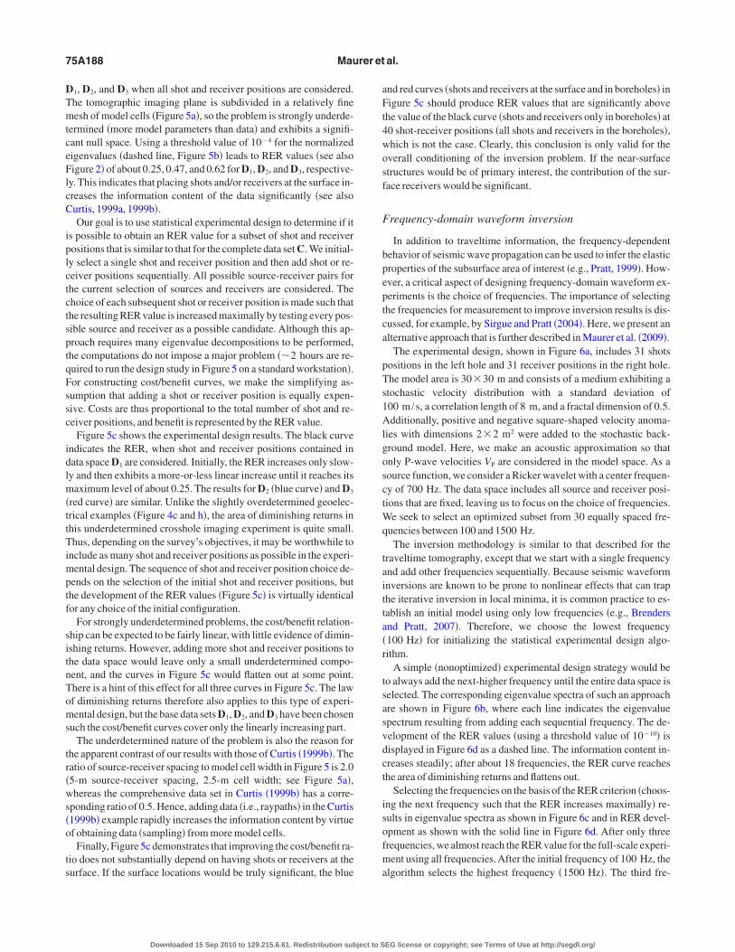
Figure 5a illustrates a simple seismic experiment to resolve theeologic structure between two parallel boreholes. Shots red dotsan be placed in the borehole on the left or at the surface, whereas re-eivers blue circles are installed in the borehole to the right or at theurface. All useful shot-receiver combinations can be subdividednto three different categories: i shots in the left borehole and re-eivers in the right borehole, ii shots in the left borehole and receiv-rs at the surface, or iii shots at the surface and receivers in the rightorehole. With these subsets, we form three data spaces: D1 i,2 i ii, and D3 i ii iii. The geologic propertiesf the medium between the boreholes are assumed to be homoge-eous, meaning that the rays between shots and receivers can beodeled with straight lines for computing the traveltime sensitivi-

ies. Each of the three data sets includes 20 shot and receiver posi-ions, which results in 400 traveltimes 1200 traveltimes for all threeata sets. The model cells have a width of 2.5 m, and the total num-er of cells is thus 40401600.

Figure 5b shows the eigenvalue spectra of FTF the data covari-nce matrix CD

1 is assumed to be a unity matrix in this example for

Dep

th(m

)N

orm

aliz

edei

genv

alue

80Normalized eigenvalue index

0

20

40

60

80

100

010

–110

–210

–310

–410

Distance (m)0 50 100

RE

R

1.0

0.9

0.8

0.7

0.6

0.5

0.4

0.3

0.2

0.1

0.0

Number of shot/receiver positions0 20 40 600 0.5 1

)

)

c)

igure 5. Survey design for seismic traveltime crosshole tomogra-hy. a Experimental layout. Red dots indicate shot, and blue circlesndicate receiver positions. The model grid is depicted with blackines. b Normalized eigenvalue spectra for A sources in left bore-ole and receivers in right borehole black, B sources in left bore-ole and receivers in right borehole and at the surface blue, and Cources in left borehole and at the surface and receivers in right bore-ole and at the surface red. c Cost/benefit curves for optimizedxperiments using data space A black, B blue, and C red.


DTmtceFlcC

iplctctsptqFssc

idlmttTimptf

sitnToms

trwso

ts

aFt4wosf

F

bpeptca

pTs1AlgosctWq

taittar

tsasvdct

isofma


1, D2, and D3 when all shot and receiver positions are considered.he tomographic imaging plane is subdivided in a relatively fineesh of model cells Figure 5a, so the problem is strongly underde-

ermined more model parameters than data and exhibits a signifi-ant null space. Using a threshold value of 104 for the normalizedigenvalues dashed line, Figure 5b leads to RER values see alsoigure 2 of about 0.25, 0.47, and 0.62 for D1, D2, and D3, respective-

y. This indicates that placing shots and/or receivers at the surface in-reases the information content of the data significantly see alsourtis, 1999a, 1999b.Our goal is to use statistical experimental design to determine if it

s possible to obtain an RER value for a subset of shot and receiverositions that is similar to that for the complete data set C. We initial-y select a single shot and receiver position and then add shot or re-eiver positions sequentially. All possible source-receiver pairs forhe current selection of sources and receivers are considered. Thehoice of each subsequent shot or receiver position is made such thathe resulting RER value is increased maximally by testing every pos-ible source and receiver as a possible candidate. Although this ap-roach requires many eigenvalue decompositions to be performed,he computations do not impose a major problem 2 hours are re-uired to run the design study in Figure 5 on a standard workstation.or constructing cost/benefit curves, we make the simplifying as-umption that adding a shot or receiver position is equally expen-ive. Costs are thus proportional to the total number of shot and re-eiver positions, and benefit is represented by the RER value.

Figure 5c shows the experimental design results. The black curvendicates the RER, when shot and receiver positions contained inata space D1 are considered. Initially, the RER increases only slow-y and then exhibits a more-or-less linear increase until it reaches its

aximum level of about 0.25. The results for D2 blue curve and D3

red curve are similar. Unlike the slightly overdetermined geoelec-rical examples Figure 4c and h, the area of diminishing returns inhis underdetermined crosshole imaging experiment is quite small.hus, depending on the survey’s objectives, it may be worthwhile to

nclude as many shot and receiver positions as possible in the experi-ental design. The sequence of shot and receiver position choice de-

ends on the selection of the initial shot and receiver positions, buthe development of the RER values Figure 5c is virtually identicalor any choice of the initial configuration.

For strongly underdetermined problems, the cost/benefit relation-hip can be expected to be fairly linear, with little evidence of dimin-shing returns. However, adding more shot and receiver positions tohe data space would leave only a small underdetermined compo-ent, and the curves in Figure 5c would flatten out at some point.here is a hint of this effect for all three curves in Figure 5c. The lawf diminishing returns therefore also applies to this type of experi-ental design, but the base data sets D1, D2, and D3 have been chosen

uch the cost/benefit curves cover only the linearly increasing part.The underdetermined nature of the problem is also the reason for

he apparent contrast of our results with those of Curtis 1999b. Theatio of source-receiver spacing to model cell width in Figure 5 is 2.05-m source-receiver spacing, 2.5-m cell width; see Figure 5a,hereas the comprehensive data set in Curtis 1999b has a corre-

ponding ratio of 0.5. Hence, adding data i.e., raypaths in the Curtis1999b example rapidly increases the information content by virtuef obtaining data sampling from more model cells.

Finally, Figure 5c demonstrates that improving the cost/benefit ra-io does not substantially depend on having shots or receivers at theurface. If the surface locations would be truly significant, the blue


nd red curves shots and receivers at the surface and in boreholes inigure 5c should produce RER values that are significantly above

he value of the black curve shots and receivers only in boreholes at0 shot-receiver positions all shots and receivers in the boreholes,hich is not the case. Clearly, this conclusion is only valid for theverall conditioning of the inversion problem. If the near-surfacetructures would be of primary interest, the contribution of the sur-ace receivers would be significant.

requency-domain waveform inversion

In addition to traveltime information, the frequency-dependentehavior of seismic wave propagation can be used to infer the elasticroperties of the subsurface area of interest e.g., Pratt, 1999. How-ver, a critical aspect of designing frequency-domain waveform ex-eriments is the choice of frequencies. The importance of selectinghe frequencies for measurement to improve inversion results is dis-ussed, for example, by Sirgue and Pratt 2004. Here, we present anlternative approach that is further described in Maurer et al. 2009.

The experimental design, shown in Figure 6a, includes 31 shotsositions in the left hole and 31 receiver positions in the right hole.he model area is 3030 m and consists of a medium exhibiting atochastic velocity distribution with a standard deviation of00 m /s, a correlation length of 8 m, and a fractal dimension of 0.5.dditionally, positive and negative square-shaped velocity anoma-

ies with dimensions 22 m2 were added to the stochastic back-round model. Here, we make an acoustic approximation so thatnly P-wave velocities VP are considered in the model space. As aource function, we consider a Ricker wavelet with a center frequen-y of 700 Hz. The data space includes all source and receiver posi-ions that are fixed, leaving us to focus on the choice of frequencies.

e seek to select an optimized subset from 30 equally spaced fre-uencies between 100 and 1500 Hz.

The inversion methodology is similar to that described for theraveltime tomography, except that we start with a single frequencynd add other frequencies sequentially. Because seismic waveformnversions are known to be prone to nonlinear effects that can traphe iterative inversion in local minima, it is common practice to es-ablish an initial model using only low frequencies e.g., Brendersnd Pratt, 2007. Therefore, we choose the lowest frequency100 Hz for initializing the statistical experimental design algo-ithm.

A simple nonoptimized experimental design strategy would beo always add the next-higher frequency until the entire data space iselected. The corresponding eigenvalue spectra of such an approachre shown in Figure 6b, where each line indicates the eigenvaluepectrum resulting from adding each sequential frequency. The de-elopment of the RER values using a threshold value of 1010 isisplayed in Figure 6d as a dashed line. The information content in-reases steadily; after about 18 frequencies, the RER curve reacheshe area of diminishing returns and flattens out.

Selecting the frequencies on the basis of the RER criterion choos-ng the next frequency such that the RER increases maximally re-ults in eigenvalue spectra as shown in Figure 6c and in RER devel-pment as shown with the solid line in Figure 6d. After only threerequencies, we almost reach the RER value for the full-scale experi-ent using all frequencies.After the initial frequency of 100 Hz, the

lgorithm selects the highest frequency 1500 Hz. The third fre-


qnd

oswc

ttm

EA

bfad

ms

ftrw

FvgN

Fa


uency is also chosen from the higher end of the spectrum, but it isot the second-highest frequency see Maurer et al. 2009 for moreetails.

Results of the tomographic inversions using all 30 frequencies ornly the three optimal frequencies selected by the experimental de-ign are shown in Figure 7. On the basis of the results in Figure 6, oneould expect the results to be similar, which is indeed the case. In the

entral part and in the low-velocity regions where the formal resolu-

Nor

mal

ized

eige

nval

ueN

orm

aliz

edei

genv

alue

Dep

th(m

)

Distance (m)

10

15

20

25

30

3510 15 20 25 30 35

VP (m/s)1500 2000 2500


0 0.2 0.4 0.6 0.8 1.0

010

–510

–10100 0.2 0.4 0.6 0.8 1.0


010

–510

–1010

a)

b)

c)

RE

R

Number of frequencies selected

1.0

0.5

0.00 10 20 30

d)

igure 6. Frequency-domain waveform inversion design. a Trueelocity model and shot and receiver positions. b Normalized ei-envalue spectra for progressively adding higher frequencies. cormalized eigenvalue spectra for adding optimized frequencies.

d Cost/benefit curves for adding progressively higher frequenciesdashed line and optimized frequencies solid line.


ion is quite good, the individual features are well resolved. Only inhe high-velocity region near the upper edge of the model do both to-

ograms suffer from resolution problems.

xample 3: Nonlinear experimental design — DesigningVA surveys

The amplitude of a seismic wave reflected from a subsurfaceoundary between two geological layers at depth Figure 8 is aunction of the wave’s incident angle at the boundary, the density i,nd the intrinsic properties of the elastic media i.e., for isotropic me-ia, the P-wave velocity i, and S-wave velocity i of both layers i

1,2. The recorded amplitudes of the reflected waves after geo-etric spreading effects have been accounted for are given by the

olution to the Zoeppritz equations e.g., Yilmaz, 2000.If the upper-layer parameters are known, it is possible to obtain in-

ormation about the elastic media properties 2 and 2 and the densi-y 2 of the lower layer e.g., a reservoir from measurements of theeflected P-wave amplitude at a range of incidence angles i1. The for-ard model in this case takes the form

Dep

th(m

)D

epth

(m)

Distance (m)

VP (m/s)

Distance (m)

1500 2000 2500

10

15

20

25

30

3510 15 20 25 30 35

10 15 20 25 30 35

a)

b)

10

15

20

25

30

35

igure 7. Frequency-domain waveform inversion results using all 30 frequencies and b three optimized frequencies.


wtt

glCtl

oilcwgle

otrcfts

teCltpfi

csci

MtFfa

Fdciwfe

Fvr4


A1i1 fx2, 2,2;i1,

here A1 is the amplitude of the reflected P-wave and fx is a functionhat represents a solution of the highly nonlinear Zoeppritz equa-ions.

The experimental design problem addressed by van den Berg et al.2003, 2005 attempts to find the offset between the source and a sin-le receiver that maximizes Shannon information about the lowerayer, taking account of the full nonlinearity of fx. They direct Montearlo sampling of the prior model PDF, evaluating and maximizing

he data-space entropy using the method of Shewry and Wynn1987.Although it is true that maximizing Shannon information canead to large variances, this does not occur in the van den Berg et al.2003, 2005AVO example.

Guest and Curtis 2009 introduce sequential algorithms that addne receiver at a time to the one-receiver design, using a schema sim-lar to that in equation 22. They develop a novel adaptive Monte Car-o method that, for each design parameter added, successively ex-ludes parts of design space over which the entropy was estimatedith low uncertainty to be small. Large computational efficiencyains result, as compared to van den Berg et al.’s methods. This al-ows optimal survey designs to be found for a survey with multiple10 offsets, which is enough to identify simple patterns of receiv-r spacing in optimal designs that could be used as rules of thumbheuristics for more complex designs.

Guest and Curtis 2010 apply this method to find the optimal setf incident angles i1 at the interlayer interface that best constrainshe elastic properties of a simulated reservoir from recorded P-waveeflection coefficients; source-receiver offsets at the earth’s surfaceorresponding to these optimal angles at the reflector can then beound with ray-tracing algorithms. Processing algorithms can be op-imized to focus attention e.g., noise-reduction methods and timepent by data processors on data recorded around those offsets.

By using the shaly-sand model of Goldberg and Gurevich 1998hat relates porosity, clay content, fluid saturation, and a range of oth-r petrophysical properties to VP and VS and to density, Guest andurtis 2009, 2010 find that the optimal design depends significant-

y on the reservoir’s porosity. This is easily understood by examininghe critical angles from a forward problem for oil reservoirs of loworosity uniform prior PDF is 10%–20%, medium porosity uni-orm prior PDF is 20%–30%, and high porosity uniform prior PDFs 30%–40%. Figure 9 shows the corresponding P-wave reflection

Source Receiverx

X V

di1 i1

j1

j2i2

α1,β1,ρ1

α2,β2,ρ2

igure 8. Geometry of an AVA experiment with a single interface atepth d. The distance between the source X and the receiver V isalled the offset x. At the interface, P-wave energy incident at angle1 is split into a reflected P-wave angle i1 and a P-S wave conversionangle j1 and is also transmitted into the second layer as a P-waveangle i2 and P-S-wave conversion angle j2. Amplitudes of eachave are given by the Zoeprittz equations. Properties of the subsur-

ace are density , P-wave velocity , and S-wave velocity in lay-rs 1 and 2.


oefficient ranges and demonstrates that the critical angle changesignificantly with the range of possible porosities. In particular, theritical angle is never reached by any survey design for a high-poros-ty substrate.

Using the sequential nonlinear design methods with the novelonte Carlo method, an optimal set of angles is derived to maximize

he Shannon information about the parameters of the lower layer.igure 10 shows the optimal designs for 10 incident angles selectedrom the range 0°–90° at 0.5° intervals. Three design optimizationsre performed, one for each of the three different porosity ranges in

Incident angle

1.0

0.8

0.6

0.4

0.2

0.0

–0.2

–0.4

–0.6

–0.8

–1.00 10 20 30 40 50 60 70 80 90

Ref

lect

ion

coef

ficie

nt

a)

1.0

0.8

0.6

0.4

0.2

0.0

–0.2

–0.4

–0.6

–0.8

–1.00 10 20 30 40 50 60 70 80 90

Ref

lect

ion

coef

ficie

ntb)

1.0

0.8

0.6

0.4

0.2

0.0

–0.2

–0.4

–0.6

–0.8

–1.00 10 20 30 40 50 60 70 80 90

Ref

lect

ion

coef

ficie

nt

c)

igure 9. Reflection-coefficient histograms for oil-filled reservoirelocity-density models with varying uniform prior porosity ranges.a The low-porosity reservoir 10–20%, b the medium-porosityeservoir 20–30%, and c the high-porosity reservoir 30%–0%.


Fwds1cerNcom

aadttpa

FcfFsgrig

tssdmtsi

dsi

ZCtdere1rgrrpb

Nl

mtgcted

mosostbals

FpG1ap

Fsbdat


igure 9 all other petrophysical parameters were allowed to varyithin broad ranges defined by their respective a priori probabilityistributions. As the porosity increases, so does the range of anglespanned by the selected angles. For the low-porosity model Figure0a, all angles are located within 0°–51°, with each of the two anglelusters located within 11° envelopes.As the porosity range increas-s, so does the maximum incident angle and so does the angularange of each of the two envelopes within which angles are selected.ote that the survey design for the midporosity reservoir almost pre-

ludes the measurements from the low-porosity design for the far-ffset envelopes, illustrating the importance of prior porosity infor-ation inAVAsurvey design.Comparing Figures 9 and 10, we see that the optimal designs use

ngles to obtain information from 1 near-zero incident angles and2 the critical angle or from 3 the highest-curvature region in thebsence of a critical angle. The algorithm selects incident angles thatisplay the largest sensitivity to perturbations in the elastic parame-ers of the second layer. These regions display the maximum uncer-ainty or entropy in the data PDF pd. Shewry and Wynn 1987rove that this implies maximum expected Shannon informationbout the model parameters.

The results from the 10-angle optimization can be generalized.igure 11 shows the spatially averaged density of receiver positionsalculated from the angle positions in Figure 10 for each of the dif-erent-porosity oil-saturated reservoirs Guest and Curtis, 2010.or high-porosity reservoirs dotted line, a larger proportion of theelected angles to be processed should be placed at high incident an-les around 55°. As the porosity decreases, the highest densityange also shifts to lower angles. For all cases, there is a density min-mum near 30°, identifying an information minimum around that an-le.

Guest and Curtis personal communication, 2010 are developinghe approach further by directly designing the optimal receiver den-ity curves similar to those in Figure 11 for a surface seismic AVAurvey. The receiver density curve can be encapsulated by a very fewesign parameters in this case, receiver density at the beginning,iddle, and end of the receiver line with linear interpolation be-

ween these points, leading to a fairly low 10 dimensional de-ign problem. Despite this simplicity, if an appropriate density curves designed, any number of receivers can be placed according to that

0 10 20 30 40 50 60 70 80 90

Incident angle

c)0 10 20 30 40 50 60 70 80 90

b)0 10 20 30 40 50 60 70 80 90

a)

igure 10. Experimental design for the reservoir model with varyingrior porosity ranges using 10 selected traces implementing theuest and Curtis 2009 method. a The final design for the0%–20% porosity reservoir, b the 20%–30% porosity reservoir,nd c the 30%–40% porosity reservoir. Receivers are allowed to belaced between 0° and 70° incident angle.


esign. Thus, for the first time, they have designed full 2D seismicurveys using SED methods — in this case, to find designs that max-mizeAVAreservoir information.

Interestingly the possible angle distribution is limited to 0°–30°current practice because commonly used approximations to theoeppritz equations break down at larger angles, and Guest andurtis personal communication, 2010 find that the dependence of

he design on porosity is greatly reduced. The strong dependence iserived from large changes in the critical angle with any change inxpected porosity; the lack of dependence when the reduced angularange of 0°–30° occurs is because the critical angle is almost alwaysxcluded from this angular range in realistic scenarios see Figure0, so the strongest dependence of the AVA relations on porosity isemoved from consideration. Hence, Guest and Curtis could create aeneral, approximately optimal, small-angle design, valid for alleasonable porosities and a range of other reservoir properties.Akeyesult is that this design depends strongly on the number of receiverslaced, up to about 100 receivers; thereafter, the design is fairly sta-le with respect to the number of receivers.

onlinear experimental design — Microseismic eventocation surveys

Rather than merely maximizing Shannon information, experi-ental design theory also can be used to evaluate the differences be-

ween designs by understanding the model-resolution capability ofeophysical data. Here, we evaluate one simple survey design for lo-ating microseismicity using the bifocal ambiguity measure of equa-ion 19 Winterfors and Curtis, personal communication, 2010 giv-n in equation 9, and then use the same measure to find an optimalesign.

Seismometer arrays are often used to locate and characterize seis-icity from fault movement or microseismicity from fracturing that

ccurs in the earth’s subsurface, resulting from naturally occurringtresses caused, for example, by tectonic motion and glacial reboundr from stress changes caused by fluid injection or extraction in sub-urface reservoirs. Location is usually achieved by detecting arrivalimes of seismic waves emanating from each seismic event and byack-projecting the wave energy and hence arrival times through anpproximate model representing the earth’s subsurface seismic ve-ocity or slowness the reciprocal of velocity structure. Methodsuch as migrating event energy act in a similar manner back projec-

0.7

0.6

0.5

0.4

0.3

0.2

0.1

0.00 10 20 30 40 50 60 70

Rec

eive

rde

nsity

Incident angle

igure 11. Receiver density plots calculated from the oil-reservoircenarios considered in Figures 9 and 10. The regression lines haveeen fitted to 10° moving-average results. The low-porosity10%–20% oil-reservoir density is shown by the solid line, the me-ium-porosity 20%–30% oil-reservoir density by the dashed line,nd the high-porosity 30%–40% oil-reservoir density by the dot-ed line.


tld

sggio1asnfwomttHtat

dsbbiwdbv

tmanrftt

rttafoaSdtmohoeoTlrcg

mptsrFlAsste

Fdstsrdgttt

Fso


ion but use waveform information rather than only traveltimes toocate events. This nonlinear inverse problem can result in multimo-al posteriori PDFs Qm see Lomax et al. 2009 for a review.

Intuitively, survey designs for locating and monitoring seismicityhould maximize geometric aperture of the survey to improve trian-ulation accuracy; but because of attenuation of the energy in propa-ating seismic waves, increasing aperture reduces data quality forncreased event-to-seismometer distances. Seismometer arrays areften deployed only on the surface e.g., Rabinowitz and Steinberg,990; Steinberg et al., 1995; Winterfors and Curtis, 2008 or only inborehole e.g., Curtis et al., 2004. When available, boreholes are

ometimes preferred because they offer advantages in terms of sig-al-to-noise ratio by placing sensors below the weathered near-sur-ace layers of the earth often highly attenuating to seismic waves,hich are assumed to outweigh geometric advantages that might beffered by placing sensors on the surface. However, the question re-ains as to the quantitative interpretational advantages or disadvan-

ages of monitoring from the surface or from a borehole in a horizon-ally stratified earth, even ignoring near-surface attenuation effects.ere, we examine this question using a simple example from Win-

erfors personal communication, 2010 and based on evaluating thembiguity measure of Winterfors and Curtis personal communica-ion, 2010 in equation 19.

Figure 12 is a graphical representation of the ambiguity W in amicroseismic event location problem given a two-receiver surveyesign using sensors on the surface of a 2D, horizontally stratified,eismic velocity model. The slownesses shown are the differencesetween P- and S-wave slownesses in each layer because these cane used to locate events without determining the event-source tim-ng Tarantola and Valette, 1982. The cross section measures 1000

1000 m, and it is assumed that seismicity could occur anywhereithin this cross section with a uniform prior probability. The stan-ard deviation of a priori uncertainty in layer velocities is assumed toe 100 m /s, and the traveltime data uncertainties have standard de-iations of 5 ms.

Evaluating the ambiguity measure W in equation 19 requires

0

1

0.6

0.3

Dep

th(k

m)

Horizontal position (km)

Slo

wne

ss(1

/km

)

0

1

igure 12. Bifocal ambiguity calculated for the seismic-monitoringesign shown by the two receivers squares on the surface. Colorshow the difference between S- and P-wave seismic slownesses inhe subsurface. Black lines connect pairs of locations m and m in theubsurface that would be indistinguishable given P- and S-wave ar-ival-time data recorded at the two seismometers. The width hencearkness of each line is proportional to the magnitude of the inte-rand in equation 19, i.e., to the relative contribution of these pointso the integral, and hence to precisely how ambiguous the two loca-ions are expected to be postsurvey given recorded data. The value ofhe integral in this case is W 2500 m2.


hat a double integral over model-parameter space be estimated nu-erically — in this case, using a Monte Carlo method. Winterfors

nd Curtis personal communication, 2010 provide several tech-iques that improve the efficiency of the Monte Carlo method e.g.,ecycling forward function evaluations fm by also using them form. In this case, the forward function d fm involves solvinghe eikonal equation to obtain arrival-time data d at all receiver loca-ions for any event location m.

The Monte Carlo scheme considers many pairs of points in pa-ameter space; in Figure 12, each black line connects a pair of loca-ions m and m in the subsurface encountered in the Monte Carlo in-egration that would be almost indistinguishable from P- and S-waverrival-time data recorded at the two surface seismometers, i.e.,m fm. The width of each line is proportional to the magnitudef the integrand in W in equation 19; that is, width indicates thembiguity of the two locations in the postsurvey interpretation.ome of the line widths are too small to distinguish clearly, but this iseliberate; only locations that are highly ambiguous have bold lineso indicate that they make the largest contributions to the ambiguity

easure W . Thinner lines connect locations that are still ambigu-us but which are expected to be better discriminated by the data andence provide a lower contribution to W . In this plot, the densityf the black lines therefore indicates the extent and location of mod-l-space ambiguity for a particular survey geometry, and the generalrientation of the lines indicates the direction of this ambiguity.hus, interpreting Figure 12, we see that indistinguishable seismic

ocations are confined to the top two surface layers for this particulareceiver geometry and that the overall direction in which locationsannot be distinguished is approximately vertical. The overall ambi-uity calculated for this design is W 2500 m2.

The receiver locations are then optimized such that W is mini-ized using a gradient-descent method. Receivers are allowed to be

laced on the surface or in a borehole on one edge of the cross sec-ion. Figure 13 shows a similar representation of the ambiguity in theame velocity structure as in Figure 12 but for two optimally locatedeceivers, both of which turn out to be in the borehole. Compared toigure 12, the ambiguity of event locations the density of black

ines is far more evenly distributed throughout the cross section.lso apparent is the reduced expected ambiguity for this design, as

hown by the reduced line widths; relatively few locations aretrongly ambiguous. However, we also see that the distances be-ween ambiguous event locations line lengths are generally short-r; hence, we expect that the variance in event locations postsurvey

0

1

0.6

0.3

Dep

th(k

m)

Horizontal position (km)

Slo

wne

ss(1

/km

)

0

1

igure 13. Similar to Figure 12 but for the seismic-monitoring de-ign shown by the two receivers squares in the borehole. The valuef the integral in this case is W 1000 m2.


st

tqdtabtvwccsitTh

eibips

mpencct

ofibsgwmpewtsi

oofgsnp

fsd

vscwppSs

let

lGutc

A

A

B

B

BC

C

CC

—

—

—

C

C

C

C


hould be smaller, as suggested by equation 20. Correspondingly,he overall ambiguity calculated for this design is W 1000 m2.

Nominally, the two-receiver arrays in both surveys have almosthe same geometric aperture for locating the events, yet they provideuite different degrees of ambiguity in resulting event locations. In-eed, the better of the two designs actually has lower spatial aper-ure. The dominant uncertainties in event location are vertical for anrray of surface sensors in a horizontally stratified medium. This isecause first-arriving waves from the ambiguous event locationsake approximately equal time to travel directly to an adjacent high-elocity layer and then follow similar paths horizontally along andithin that layer and then up to each seismometer. Hence, data re-

orded at such seismometers cannot distinguish between the two lo-ations. Using vertically offset borehole receivers above and belowuch high-velocity layers reduces much of this ambiguity withoutntroducing a similar ambiguity in the horizontal direction becausehe layers are geometrically orthogonal to the observation well.hus, first-arriving energy generally cannot travel within any singleigh-velocity layer to both of the receivers.

Equation 19 provides a useful and intuitive assessment of expect-d ambiguity in seismic event location and leads to designs that arentuitively reasonable. It is clear from these examples that it woulde misleading to design experiments solely on the basis of maximiz-ng apparent aperture without accounting for the effect of waveropagation in horizontally stratified subsurface velocity structures;uch a strategy would almost definitely lead to suboptimal designs.

CONCLUSIONS

Major improvements have been achieved in the field of experi-ental design during the past 15 years, both conceptually and in

ractice. For instance, the superiority of nontraditional, optimizedlectrode configurations for geoelectrical surveys is now well recog-ized. Modern data-acquisition systems allow arbitrary electrodeonfigurations to be implemented quite easily, so it is expected thatollecting geoelectrical data with optimized electrode configura-ions will soon become common practice.

Despite these successes, several concerns remain to be addressed.First, most geophysical-survey design studies have focused on

ptimizing data information content. This is certainly an importantrst step; but to truly optimize a geophysical experiment, other cost/enefit constraints must be considered. For example, for conductingeismic crosshole measurements, one may use a single boreholeeophone or a string with several geophones. A single geophoneould be relatively cheap to buy or lease, and it would allow theeasurement of quite irregular source-receiver patterns. With a geo-

hone string, many measurements could be performed much morefficiently, but the purchase or rental costs would be higher and thereould be less flexibility for choosing source-receiver patterns. Fu-

ure experimental design algorithms need to consider available in-trumentation choices as constraints and factor the associated costsn the optimization process.

Second, nonlinear experimental design is critical for a wide rangef geophysical problems because few can truly be considered linearver the range of models considered possible according to prior in-ormation. The examples presented in this paper demonstrate theeneral feasibility of nonlinear experimental design to relativelyimple problems, but more research is required before such tech-iques can be applied routinely to most practical survey-designroblems. Nevertheless, for the first time, optimal receiver density


or AVA/AVO studies has been calculated for complete 2D seismicurveys. Hence, the emergence and proof of concept of practical, in-ustrial, nonlinear design algorithms may be approaching rapidly.

Third, most survey-design algorithms, particularly nonlinearariants, are computationally expensive. This imposes severe con-traints on applications to realistic design problems. Improving theomputational efficiency of key modules that are called many timeshile executing a design algorithm is therefore critical. In linearroblems, the computation of the model resolution matrix can be im-roved dramatically using update formulas and parallel computing.imilar efficiencies will be even more important for nonlinear de-ign algorithms.

Finally, easy-to-use computer interfaces must be designed that al-ow nonspecialists to develop experimental designs, based on differ-nt scenarios involving choices in survey costing and possible varia-ions in petrophysical parameterization of earth models.

ACKNOWLEDGMENTS

This paper includes research results to which many of our col-eagues have contributed. The authors especially thank Thomasuest, Emanuel Winterfors, and Peter Stummer for providing fig-res and information describing their design methods. We also thankwo anonymous reviewers for helpful suggestions that improved thelarity of the manuscript.

REFERENCES

jo-Franklin, J., 2009, Optimal experiment design for time-lapse traveltimetomography: Geophysics, 74, no. 4, Q27–Q40, doi: 10.1190/1.3141738

tkinson, A. C., and A. N. Donev, 1992, Optimum experimental designs:Clarendon Press.

arth, N., and C. Wunsch, 1990, Oceanographic experiment design by simu-lated annealing: Journal of Physical Oceanography, 20, 1249–1263, doi:10.1175/1520-048519900201249:OEDBSA 2.0.CO;2

renders, A. J., and R. G. Pratt, 2007, Efficient waveform tomography forlithospheric imaging: Implications for realistic, two-dimensional acquisi-tion geometries and low-frequency data: Geophysical Journal Internation-al, 168, no. 1, 152–170, doi: 10.1111/j.1365-246X.2006.03096.x

utler, D. K., ed., 2005, Near-surface geophysics: SEG.oles, D., and F. Morgan, 2009, A method of fast, sequential experimentaldesign for linearized geophysical inverse problems: Geophysical JournalInternational, 178, 145–158, doi: 10.1111/j.1365-246X.2009.04156.x

oscia, I., L. Marescot, H. R. Maurer, S. A. Greenhalgh, and A. G. Green,2008, Experimental design for cross hole electrical resistivity tomographydata sets: EAGE Near-Surface Meeting.

ox, D. R., 1958, Planning of experiments: John Wiley & Sons, Inc.urtis, A., 1999a, Optimal design of focussed experiments and surveys: Geo-physical Journal International, 139, no. 1, 205–215, doi: 10.1046/j.1365-246X.1999.00947.x—–, 1999b, Optimal experiment design: Cross-borehole tomographic ex-amples: Geophysical Journal International, 136, no. 3, 637–650, doi:10.1046/j.1365-246x.1999.00749.x—–, 2004a, Theory of model-based geophysical survey and experimentaldesign, Part A — Linear problems: The Leading Edge, 23, 997–1004, doi:10.1190/1.1813346—–, 2004b, Theory of model-based geophysical survey and experimentaldesign, Part B — Nonlinear problems: The Leading Edge, 23, 1112–1117,doi: 10.1190/1.1825931

urtis, A., and A. Lomax, 2001, Prior information, sampling distributionsand the curse of dimensionality: Geophysics, 66, 372–378, doi: 10.1190/1.1444928

urtis, A., and H. R. Maurer, 2000, Optimizing the design of geophysical ex-periments — Is it worthwhile? Eos, Transactions, American GeophysicalUnion, 81, 224–225.

urtis, A., A. Michelini, D. Leslie, and A. Lomax, 2004, A deterministic al-gorithm for experimental design applied to tomographic and microseismicmonitoring surveys: Geophysical Journal International, 157, 595–606,doi: 10.1111/j.1365-246X.2004.02114.x

urtis, A., and R. Snieder, 1997, Reconditioning inverse problems using thegenetic algorithm and revised parameterization: Geophysics, 62,


C

FF

G

G

G

G

—

H

H

H

J

K

L

L

L

L

M

M

—

M

M

M

M

O

O

P

P

R

R

S

S

S

S

S

S

S

T

T

T

T

v

—

W

W

W


1524–1532, doi: 10.1190/1.1444255urtis, A., and R. Wood, 2004, Optimal elicitation of probabilistic informa-tion from experts, in A. Curtis and R. Wood, eds., Geological prior infor-mation: Informing science and engineering: Geological Society of Lon-don Special Publication 239, 127–145.

edorov, V. V., 1972, Theory of optimal experiments:Academic Press Inc.urman, A., T. P. A. Ferre, and G. L. Heath, 2007, Spatial focusing of electri-cal resistivity surveys considering geologic and hydrologic layering: Geo-physics, 72, no. 2, F65–F73, doi: 10.1190/1.2433737

lenn, W. E., and S. H. Ward, 1976, Statistical evaluation of electrical sound-ing methods, Part 1: Experimental design: Geophysics, 41, 1207–1221.

oldberg, I., and B. Gurevich, 1998, A semi-empirical velocity-porosity-clay model for petrophysical interpretation of P- and S-velocities: Geo-physical Prospecting, 46, 271–285.

riffiths, D. H., and J. Turnbull, 1985, A multi-electrode array for resistivitysurveying: First Break, 3, no. 7, 16–20.

uest, T., and A. Curtis, 2009, Iteratively constructive sequential design ofexperiments and surveys with nonlinear parameter-data relationships:Journal of Geophysical Research, 114, B04307, doi: 10.1029/2008JB005948—–, 2010, Optimal trace selection for amplitude-variation-with-angleAVA processing of shale-sand reservoirs: Geophysics, 75, no. 4, doi:10.1190/1.3462291.

aber, E., L. Horesh, and L. Tenorio, 2008, Numerical methods for experi-mental design of large-scale linear ill-posed inverse problems: InverseProblems, 24, 055012.

ardt, M., and F. Scherbaum, 1994, The design of optimum networks for af-tershock recordings: Geophysical Journal International, 117, 716–726,doi: 10.1111/j.1365-246X.1994.tb02464.x

ennig, T., A. Weller, and M. Moller, 2008, Object orientated focussing ofgeoelectric multielectrode measurements: Journal ofApplied Geophysics,65, no. 2, 57–64, doi: 10.1016/j.jappgeo.2008.04.007

ones, A. G., and J. H. Foster, 1986, An objective real-time data-adaptivetechnique for efficient model resolution improvement in magnetotelluricstudies: Geophysics, 51, 90–97, doi: 10.1190/1.1442043

ijko, A., 1977, An algorithm for the optimal distribution of a regional seis-mic network — I: Pure and Applied Geophysics, 115, 999–1009, doi:10.1007/BF00881222

iner, C. L., W. D. Underwood, and R. Gobeli, 1999, 3-D seismic survey de-sign as an optimization problem: The Leading Edge, 18, 1054–1060.

oke, M. H., and R. D. Barker, 1996, Practical techniques for 3D resistivitysurveys and data inversion: Geophysical Prospecting, 44, no. 3, 499–523,doi: 10.1111/j.1365-2478.1996.tb00162.x

oke, M. H., and P. Wilkinson, 2009, Rapid parallel computation of opti-mised arrays for electrical imaging surveys: EAGE Near-Surface Confer-ence, Proceedings, B11.

omax, A., A. Michelini, and A. Curtis, 2009, Earthquake location, direct,global-search methods: in R. A. Meyers, ed., Encyclopedia of complexityand system science: Springer.atsu’ura, M., and N. Hirata, 1982, General least-squares solutions to quasi-linear inverse problems with a priori information: Journal of Physics of theEarth, 30, 451–468.aurer, H. R., and D. E. Boerner, 1998a, Optimized and robust experimentaldesign:Anon-linear application to EM sounding: Geophysical Journal In-ternational, 132, no. 2, 458–468, doi: 10.1046/j.1365-246x.1998.00459.x—–, 1998b, Optimized design of geophysical experiments: The LeadingEdge, 17, 1119.aurer, H. R., D. E. Boerner, and A. Curtis, 2000, Design strategies for elec-tromagnetic geophysical surveys: Inverse Problems, 16, no. 5, 1097–1118,doi: 10.1088/0266-5611/16/5/302aurer, H. R., S. A. Greenhalgh, and S. Latzel, 2009, Frequency and spatialsampling strategies for crosshole seismic waveform spectral inversion ex-periments: Geophysics, 74, no. 6, WCC11–WCC21.enke, W., 1984, Geophysical data analysis: Discrete inverse theory: Aca-demic Press Inc.itchell, T. J., 1974, An algorithm for the construction of ‘D-optimal’exper-
Y

imental designs: Technometrics, 16, no. 2, 203–210, doi: 10.2307/1267940

ldenborger, G. A., and P. S. Routh, 2009, The point-spread function mea-sure of resolution for the 3-D electrical resistivity experiment: Geophysi-cal Journal International, 176, 405–414, doi: 10.1111/j.1365-246X.2008.04003.x

ldenburg, D. W., 1978, The interpretation of direct current resistivity mea-surements: Geophysics, 43, 610–625, doi: 10.1190/1.1440840

ratt, R. G., 1999, Seismic waveform inversion in the frequency domain, Part1: Theory and verification in a physical scale model: Geophysics, 64,888–901, doi: 10.1190/1.1444597

ress, W. H., S. A. Teukolsky, W. T. Vetterling, and B. P. Flannery, 2007, Nu-merical recipes: The art of scientific computing, 3rd ed.: Cambridge Uni-versity Press.

abinowitz, N., and D. M. Steinberg, 1990, Optimal configuration of a seis-mographic network: A statistical approach: Bulletin of the SeismologicalSociety ofAmerica, 80, no. 1, 187–196.

outh, P. S., G. A. Oldenborger, and D. W. Oldenburg, 2005, Optimal surveydesign using the point spread function measure of resolution: 75th AnnualInternational Meeting, SEG, ExpandedAbstracts, 1033–1036.

hannon, C. E., 1948, A mathematical theory of communication: The BellSystem Technical Journal, 27, 379–423, 623–656.

hewry, M. C., and H. P. Wynn, 1987, Maximum entropy sampling: Journalof Applied Statistics, 14, no. 2, 165–170, doi: 10.1080/02664768700000020

irgue, L., and R. G. Pratt, 2004, Efficient waveform inversion and imaging:A strategy for selecting temporal frequencies: Geophysics, 69, 231–248,doi: 10.1190/1.1649391

tark, P. B., 2008, Generalizing resolution: Inverse Problems, 24, no. 3,034014, doi: 10.1088/0266-5611/24/3/034014

teinberg, D. M., N. Rabinowitz, Y. Shimshoni, and D. Mizrachi, 1995, Con-figuring a seismographic network for optimal monitoring of fault lines andmultiple sources: Bulletin of the Seismological Society of America, 85,1847–1857.

tummer, P., H. R. Maurer, and A. G. Green, 2004, Experimental design:Electrical resistivity data sets that provide optimum subsurface informa-tion: Geophysics, 69, 120–139, doi: 10.1190/1.1649381

tummer, P., H. R. Maurer, H. Horstmeyer, and A. G. Green, 2002, Optimi-zation of DC resistivity data acquisition: Real-time experimental designand a new multielectrode system: IEEE Transactions on Geoscience andRemote Sensing, 40, 2727–2735, doi: 10.1109/TGRS.2002.807015

aguchi, G., 1987, Systems of experimental design volumes 1 and 2 1976and 1977 with 1987 translation: UNIPUB.

arantola, A., 2005, Inverse problem theory and methods for model parame-ter estimation: Society for Industrial andApplied Mathematics.

arantola, A., and B. Valette, 1982, Generalized nonlinear problems solvedusing the least squares criterion: Reviews of Geophysics, 20, no. 2,219–232, doi: 10.1029/RG020i002p00219

elford, W. M., L. P. Geldart, and R. E. Sheriff, 1990, Applied geophysics:Cambridge University Press.

an den Berg, J., A. Curtis, and J. Trampert, 2003, Bayesian, nonlinear exper-imental design applied to simple, geophysical examples: GeophysicalJournal International, 55, 411–421.—–, 2005, Correction to Bayesian, nonlinear experimental design appliedto simple, geophysical examples: Geophysical Journal International, 161,no. 2, 265–265.ilkinson, P., P. Meldrum, J. Chambers, O. Kuras, and R. Ogilvy, 2006, Im-proved strategies for the automatic selection of optimized sets of electricalresistivity tomography measurement configurations: Geophysical JournalInternational, 167, 1119–1126, doi: 10.1111/j.1365-246X.2006.03196.xinterfors, E., and A. Curtis, 2008, Numerical detection and reduction ofnon-uniqueness in nonlinear inverse problems: Inverse Problems, 24, no.025016.olpert, D. H., and W. G. Macready, 1997, No free lunch theorems for opti-mization: IEEE Transactions on Evolutionary Computation, 1, no. 1,67–82.

ilmaz, O., 2000, Seismic data processing: SEG.


Documents

Recent advances in optimized geophysical survey … advances in optimized geophysical survey design ... Appropriate survey design is therefore critical to justify the ... applicable