Embed Size (px)
Citation preview

Recent contrasting winter temperature changes over North
America linked to enhanced positive Pacific North American
pattern
Zhongfang Liu1, Zhimin Jian1, Kei Yoshimura2, Nikolaus H. Buenning3, Christopher J. Poulsen4, and Gabriel J.
Bowen5
1State Key Laboratory of Marine Geology, Tongji University, Shanghai, 200092, China, 2Atmosphere and Ocean
Research Institute, University of Tokyo, Kashiwa, Chiba 2778568, Japan, 3Department of Earth Sciences,
University of Southern California, Los Angeles, California 90089, USA, 4Department of Earth and Environmental
Sciences, University of Michigan, Ann Arbor, Michigan 48109, USA, 5Department of Geology and Geophysics
and Global Change and Sustainability Center, University of Utah, Salt Lake City, Utah 84112, USA
Corresponding author: Zhongfang Liu,
School of Ocean and Earth Science, Tongji University
1239 Siping Road, Yangpu District, Shanghai, 200092, China
Email: [email protected]
Tel: 86-18616700653
This article is protected by copyright. All rights reserved.
This is the author manuscript accepted for publication and has undergone full peer review but hasnot been through the copyediting, typesetting, pagination and proofreading process, which maylead to differences between this version and the Version of Record. Please cite this article as doi:10.1002/2015GL065656

Abstract
Recently enhanced contrasts in winter (DJF) mean temperatures and extremes (cold
southeast and warm northwest) across North America have triggered intensive
discussion both within and outside of the scientific community, but the mechanisms
responsible for these contrasts remain unresolved. Here we use a combination of
observations and reanalysis datasets to show that the strengthened contrasts in winter
mean temperatures and extremes across North America are closely related to an
enhancement of the positive Pacific-North American (PNA) pattern during the second
half of the twentieth century. Recent intensification of positive PNA events is
associated with amplified planetary waves over North America, driving cold-air
outbreaks into the southeast and warm tropical/subtropical air into the northwest. This
not only results in a strengthened winter mean temperature contrast, but increases the
occurrence of the opposite-signed extremes in these two regions.
This article is protected by copyright. All rights reserved.
1. Introduction
Instrumental and historical records reveal a pronounced global warming since the
1850s [Hansen et al., 2010]. Against the backdrop of global warming, the northwest
(NW) regions of North American show a persistent winter warming, whereas a slight
cooling persists in the southeastern (SE) parts of the continent (Figures 1a and 1b).
This cooling region has been referred to as a “warming hole” [Kunkel et al., 2006;
Pan et al., 2004], and has led to a geographically prominent contrast in mean
temperature anomalies between the NW and SE [Meehl et al., 2012]. These
contrasting trends were further strengthened during the second half of the
twentieth century (Figure 1b). Along with this NW-SE contrast in mean temperature
trends, there has also been an increase in cold extremes in the SE and warm extremes
in the NW during the winter months. For example, during the past two winters, the
central and eastern USA were struck by ferocious blizzards and record-breaking low
temperatures, whereas western states experienced some of the warmest winters on
record [Greene, 2012; Masters, 2014]. These temperature extremes have had a
substantial impact on the environment (e.g., declined snowpack [Pederson et al., 2011]
This article is protected by copyright. All rights reserved.

and increased forest wildfire [Westerling et al., 2006] in the mountainous regions) and
economy in North America [Greene, 2012; Masters, 2014].
The underlying mechanisms responsible for these regional temperature trends still
remain a subject of debate. Observations and simulations suggest that SST variability
driven by the El Niño Southern Oscillation (ENSO), the Pacific Decadal Oscillation
(PDO) and the Atlantic Multidecadal Oscillation (AMO) may partially contribute to
the differences in regional temperature trends [Kunkel et al., 2006; Meehl et al., 2012;
Pan et al., 2013; Robinson et al., 2002]. Recent studies have argued that the contrast
in mean temperature is due largely to changes in atmospheric circulation, including a
wavier jet stream and amplified atmospheric planetary waves [Cohen et al., 2014;
Kaspi and Schneider, 2011; Shepherd, 2014]. These atmospheric circulation changes
have also been linked to weather extremes (heat waves, severe cold and heavy
snowstorms, etc) in the Northern Hemisphere mid-latitudes [Cohen et al., 2014;
Francis and Vavrus, 2012; 2015; Petoukhov et al., 2013; Screen and Simmonds, 2014;
Tang et al., 2014]. During winter, the dominant atmospheric circulation pattern over
North America consists of a ridge over the Rocky Mountains and a trough over
southeastern United States. This ridge-trough system, referred to as the Pacific North
American (PNA) pattern [Wallace and Gutzler, 1981], represents the structure of a
quasi-stationary planetary wave system over the North Pacific and North America
sectors. A positive (negative) PNA pattern is associated with amplified (dampened)
This article is protected by copyright. All rights reserved.

planetary waves, as expressed by an enhanced (weakened) ridge-trough pattern over
North America. Instrumental records and reconstructions indicate a trend towards the
positive PNA state since the mid-1850s [Hubeny et al., 2011; Moore et al., 2002;
Trouet and Taylor, 2010]. Given the well-documented association between the PNA
and both synoptic weather patterns [Wallace and Gutzler, 1981] and winter climates
[Leathers et al., 1991], we speculate that the recent intensification of NW-SE
temperature contrasts is linked to an enhanced positive PNA pattern. In this study we
use a combination of observations and reanalysis datasets to explore the link between
the PNA pattern and winter mean temperature anomalies and extremes over North
America.
2. Data and Methods
2.1. Observations and Reanalysis Data
We used the surface temperature from the CRU TS 3.22 [Harris et al., 2014] and
CRUTEM4 [Jones et al., 2012] and data sets provided by the Climatic Research Unit
(http://www.cru.uea.ac.uk/data). CRU TS 3.22 data provides monthly mean land
surface temperature from 1901 to 2013 on a 0.5°×0.5° grid, and is constructed
through interpolation of instrumental measurements. CRUTEM4 is a gridded dataset
of global historical near-surface air temperature anomalies over land, and data are
available for each month from January 1850 to present, on a 5° grid. Winter means
are calculated by averaging the monthly means of December through February (DJF),
This article is protected by copyright. All rights reserved.

which yielded 111 and 114 complete winters for CRU TS 3.22 and CRUTEM4,
respectively. The Global Historical Climatology Network Monthly (GHCN-M)
temperature dataset [Lawrimore et al., 2011] is also used for comparison in this study.
ENSO variability was measured using the Niño 3.4 index, defined as the SST
anomaly averaged over the region 5°N–5°S, 170°W–120°W. The monthly Niño 3.4
index is calculated from the Hadley Centre HadISST1 dataset [Rayner et al., 2003],
and can be obtained at http://www.metoffice.gov.uk/hadobs/hadisst. Winter means of
the Niño 3.4 index from 1902 to 2015 are used in this study.
The 500-hPa geopotential height data from the Twentieth Century Reanalysis version
2 (20CRv2; http://www.esrl.noaa.gov/psd/data/gridded) [Compo et al., 2011] was
used to depict changes in the atmospheric circulation pattern. This dataset is the
newest reanalysis to produce comprehensive atmospheric fields based on
observational constraints from 1871 to 2012 on a 2° × 2° global grid. For comparison,
we also show the 500-hPa geopotential height data from the NCEP/NCAR reanalysis
dataset version 1 (NCEP 1; http://www.esrl.noaa.gov/psd/data/gridded/) [Kalnay et al.,
1996] for the period 1948-2015. Surface temperature and wind fields from the NCEP
1 were also used to explore the influence of the atmospheric circulation pattern on
temperature.
2.2. Winter Temperature Trends and Extremes
The spatial trend patterns of the winter temperature expressed as °C per decade for
This article is protected by copyright. All rights reserved.

each gridcell are calculated by fitting a slope line using a least squares fit separately
for the periods 1902–2012 (Figure 1a) and 1949–2012 (Figure 1b; for comparison
with observational record of winter PNA). Based on the spatial patterns of the winter
temperature trends, we define two poles with maximum absolute slopes at
mid-latitudes: a SE pole spanning 30°N–40°N and 95°W–75°W, (red box in Figures
1a and 1b), and a NW pole spanning 45°N–60°N and 130°W–100°W (blue box in
Figures 1a and 1b). To examine the spatial contrast in temperature, a large-scale
NW-SE temperature gradient (∆T = TNW Anomaly – TSE Anomaly; Figure 1c) is
computed from the difference in average temperature anomaly over the NW and SE
boxed regions. A least-squares linear trend in ∆T is used as a concise metric of the
long-term change in temperature contrast between the NW and SE. To define the
temperature extremes, the ∆T values are subjectively segregated according to the
quintiles of the standardized ∆T. Winters with ∆T values above the upper quintile are
defined as positive-extreme winters, which represent cold winters in the SE and warm
winters in the NW. Winters with ∆T values below the lower quintile are defined as
negative-extreme winters, representing hot winters in the SE and cold winters in the
NW. We identify 22 winters with anomalous positive ∆T values and 26 winters with
anomalous negative ∆T values from the 114 winters.
2.3. PNA Index
To measure the strength of the PNA, monthly PNA indices for both 20CRv2 and
This article is protected by copyright. All rights reserved.

NCEP 1 datasets are constructed according to a modified point-wise method
developed by the Climate Prediction Center (CPC):
𝑃𝑁𝐴 = 𝑍𝑍∗(15°N– 25°N, 180°– 140°W) − 𝑍𝑍∗(40°N– 50°N, 180°– 140°W)
+ 𝑍𝑍∗(45°N– 60°N, 125°W– 105°W)− 𝑍𝑍∗(25°N– 35°N, 90°W– 70°W) (1)
Where 𝑍𝑍∗ is the monthly mean 500-hPa geopotential height anomaly that is
computed as the departures from the 1950-2000 monthly climatology. Winter mean
PNA indices are calculated from the average PNA index from December through
February. All calculated winter PNA index time series are shown in Figure 1d, which
shows that the 20CRv2 PNA index are highly correlated with the NCEP 1 PNA index
(r2 = 0.99, 1949-2012 years) and both are highly correlated with the observations
during the period 1951-2015 (r2 = 0.98 and 0.99, respectively). Winters with PNA
index more than one standard deviation above (>1σ) and below (<-1σ) the
climatological mean are defined as positive and negative PNA winters, respectively.
Based on this criterion, we identified 20 positive and 20 negative PNA winters during
period 1902-2015.
2.4. Occurrence rate estimation of extreme events
The occurrence rates of winter temperature extremes and PNA events are estimated
over the period 1902-2015 using a Gaussian kernel technique [Mudelsee et al., 2003].
This approach can estimate time-dependent event occurrence rates and assess the
significance of trends via bootstrap confidence bands. The occurrence rate (𝜆) at time
This article is protected by copyright. All rights reserved.

(t) can be determined as
𝜆(𝑡) = ℎ−1 ∑ 𝐾 �𝑡−𝑇(𝑖)ℎ
�𝑖 (2)
where K is the kernel function and h is the bandwidth. 𝑇(𝑖) is the total number of
events (i=1,…, N). We used the program XTREND [Mudelsee, 2002] to estimate the
occurrence rate.
3. Results
3.1. Contrasting Winter Temperature Trends
Figure 1 shows the trends in winter mean surface temperatures for the periods
1902-2012 (Figure 1a) and 1949-2012 (Figure 1b). The most striking feature is the
contrasting regional trends since the 1900s, with increasing mean temperatures over
the NW and decreasing mean temperatures over the SE. These contrasting trends are
enhanced since the 1950s (Figure 1b). At mid-latitudes, winter warming in the NW is
+0.23 ± 0.06°C decade-1 (p < 0.001) over the 1902–2015 period, and 0.46 ± 0.14°C
decade-1 (p < 0.001) over the 1949–2015 period (Figures 1a and S1a), which is greater
than the Northern Hemisphere mean (0.11°C decade-1) [Jones et al., 2012]. In contrast,
the SE shows no warming or a slight cooling (Figures 1a, 1b and S1b). The warming
in the NW and cooling in the SE have led to a strengthened contrast in mean
temperature anomalies across North America, as revealed by a significant (p < 0.005)
increase in ∆T (Figure S1c).
During the same period, the PNA index shows a clear increase, especially over the
This article is protected by copyright. All rights reserved.

period 1949-2015 (p < 0.05) (Figure S1d). The trend and variability of observed ∆T
are consistent with those of the PNA index (Figures 1c and 1d). The PNA index
accounts for 74% and 80% of the ∆T variance over the periods 1902-2015 and
1949-2015, respectively, and explains a greater share of the ∆T variance than any of
the SST-associated climate indices (Figure S2). Our analysis strongly suggests that
the NW-SE temperature anomaly gradient across North America is likely due to
recent strengthening of the positive PNA pattern. This strengthening of the positive
PNA leads to a wavier polar jet characterized by a ridge of high pressure over the NW
(Figure S3b) and a trough of low pressure over the SE (Figure S3a).
3.2 Contrasting Winter Temperature Extremes
The strengthened NW-SE winter temperature differences are reflected not only in the
mean trends but also in the extremes (Figures 1a-1c). The ∆T time series shows that
the extreme negative ∆T values mostly occurred during the first half of the twentieth
century, while the extreme positive ∆T values have increased since 1950s (Figure 1c).
These east-west contrasting temperature extremes across the United States have been
captured by climate-model simulations [Meehl et al., 2012], and opposite-signed
extremes have been observed over other continents and were attributed to similar
mechanisms [Screen and Simmonds, 2014; Shepherd, 2014]. Previous studies have
suggested that the rise in the number of cold/warm extremes can be explained by a
shift in the mean to either colder or warmer temperatures [Coumou et al., 2014;
This article is protected by copyright. All rights reserved.

Rahmstorf and Coumou, 2011]. Thus, the trends in both means and extremes may
share a common underlying cause. This is corroborated by consistent changes in
temperature extremes and PNA events (Figures 1c and 1d), supporting previous work
that demonstrated that high-amplitude planetary waves can be key drivers for
generating extreme events [Cohen et al., 2014; Francis and Vavrus, 2012; 2015;
Petoukhov et al., 2013; Screen and Simmonds, 2014; Tang et al., 2014].
To test the hypothesis that PNA-like variation in the circulations associated with
opposite-signed temperature gradient extremes over North America, we examine
composite anomalies of the wintertime 500-hPa geopotential heights for periods of
anomalous positive and negative ∆T (Figure 2). For extreme positive ∆T (warm NW
and cold SE) winters during both the 1902-2012 and 1949-2015 periods, significant (p
< 0.05) positive height anomalies occur over the Hawaiian Islands and the western
interior of North America, and negative height anomalies over the Aleutian Islands
and the southeastern United States (Figures 2a and 2c). This pattern is consistent with
the positive phase of the conventional PNA [Wallace and Gutzler, 1981]. Moreover,
the composite anomalies associated with extreme negative ∆T (cold NW and warm
SE) mimic a negative PNA pattern (Figures 2b and 2d). A similar pattern is also
found after removing ENSO events from the composite (Figure S4). The influence of
the PNA and ENSO on the temperature extremes is further distinguished by
examining probability density functions (PDFs) of the PNA and the Niño 3.4 indices
This article is protected by copyright. All rights reserved.

during the winters with extreme ∆T values (Figure 3). Winters with extreme positive
(negative) ∆T are strongly linked to the positive (negative) PNA pattern (Figures 3a
and 3c). In contrast, the influence of the ENSO on ∆T appears weak, except for the
winters with extreme positive ∆T, in which a warm phase of the ENSO is more likely
to occur (Figure 3b).
The ∆T time series also reveals a shift in the spatial pattern of winter temperature
extremes over North America (Figure 1c). Occurrence rates of extreme ∆T values
based on the Gaussian kernel technique [Mudelsee et al., 2003] shows a significant (p
= 0.05) increase in the number of extreme positive ∆T anomalies during the twentieth
century, with the highest frequency (0.28 times yr-1) occurring in the late 1970s
(Figure 4a). The increasing frequency of positive ∆T anomalies is matched with a
significant (p = 0.05) increase in the occurrence of positive PNA events, with the
highest frequency (0.23 times yr-1) also occurring during the late 1970s (Figure 4b).
Similarly, the latter part of the 20th century was characterized by decreasing
occurrences of extreme negative ∆T winters and negative PNA events (Figures S5a
and S5b). The occurrence rate of negative ∆T anomalies decreased since mid-1920s,
with a dramatic decrease in 1970s, which to a large extent matches with the
occurrence rate of the negative PNA events. Thus both the spatial structure and
temporal trends in NW-SE oriented temperature extremes appear to be closely linked
to changes in the PNA circulation pattern throughout the 20th and early 21th
This article is protected by copyright. All rights reserved.
centuries.
4. Conclusions and Discussion
We have demonstrated that recent contrasting winter average temperatures and extremes
over North America are closely linked to enhanced positive Pacific North American
pattern. An intensification of the positive PNA patter drives strong cold-air outbreaks
into the SE, but advects more tropical/subtropical air to the NW, which not only causes
a strengthened contrast in mean temperature between the NW and SE, but also increases
the occurrence of the opposite-signed temperature extremes in these two regions. These
findings provide new evidence that amplified planetary waves contribute to the contrast in
mid-latitude winter mean temperature anomalies [Kaspi and Schneider, 2011; Meehl et
al., 2012] and extremes [Screen and Simmonds, 2014; Shepherd, 2014] between the
eastern and western margins of continents. Though recent intensification of positive
PNA phases underscores the need for a more complete understanding of the
circulation response to external forcing, present findings may provide a consistent
framework for detection and attribution of past climate change [Liu et al., 2014] and
future prediction of winter climatological temperatures across North America.
The circulation patterns associated with positive and negative PNA phases provide a
plausible mechanism for shifts in mean NW-SE temperature anomaly contrasts as
well as variation in the occurrence of extreme ∆T. The amplified ridge over the NW
and trough over the SE during the positive phase of the PNA drive strong cold-air
This article is protected by copyright. All rights reserved.

outbreaks into the SE, substantially increasing the frequency of cold temperature
extreme in the region (Figures S3b and S3d). Also, this circulation pattern advects
more tropical/subtropical air to the NW, yielding abnormally warm winters in this
region (Figures S3b and S3d). Conversely, during the negative PNA phase the
combination of a ridge over the Gulf of Alaska and a trough over the NW leads to
more frequent intrusions of maritime polar and arctic air masses into the NW,
generating cold temperature extremes. A ridge and the northward migration of the
polar jet over the SE allows more frequent advection of tropical/subtropical air masses,
leading to warm temperature extremes during the negative PNA winters (Figures S3a
and S3c).
Though the contrasts in mean temperature anomalies and extreme winters are largely
associated with a naturally occurring mode of atmospheric variability, anthropogenic
forcing may indirectly strengthen these contrasts. The extended PNA history and
proxy-based reconstructions [Hubeny et al., 2011; Moore et al., 2002; Trouet and
Taylor, 2010] reveal a significant trend towards a positive PNA phase, and an
increased frequency of positive PNA events. Though the physical mechanisms
leading to enhanced positive PNA remain unclear, recent studies have suggested that
rapid Arctic warming has caused a wavier jet stream and amplified planetary waves
[Cohen et al., 2014; Francis and Vavrus, 2012; 2015; Mori et al., 2014; Petoukhov et
al., 2013; Screen and Simmonds, 2014; Tang et al., 2014], albeit with some
This article is protected by copyright. All rights reserved.

uncertainties [Barnes, 2013; Screen and Simmonds, 2013a; b]. Given this link, the
recent persistent positive PNA pattern may be a response to anthropogenic forced
Arctic warming. The increase towards a positive PNA pattern since the mid-twentieth
century has resulted in warmer temperatures in the NW relative to the SE, as well as
more frequent extreme winters of cold SE and warm NW, yielding a stronger
temperature change contrasts between the two regions.
Acknowledgements
We thank H. Shimazaki for providing help with the Gaussian kernel technique. This
work was supported by National Natural Science Foundation of China (grant
41171022) and the China Young 1000-Talent Program. The CRU TS 3.22 and
CRUTEM4 temperature data were provided by the Climatic Research Unit
(http://www.cru.uea.ac.uk/data). The GHCN-M temperature data was obtained from
the National Climatic Data Center (https://www.ncdc.noaa.gov/ghcnm/). HadISST1
sea-surface temperature data was obtained from the Hadley Centre, U.K.
Meteorological Office (http://www.metoffice.gov.uk/hadobs/hadisst/). The
geopotential height data from the 20CRv2 and the NCEP/NCAR reanalysis were
provided by the NOAA/OAR/ESRL PSD, Boulder, Colorado, USA
(http://www.esrl.noaa.gov/psd/data/gridded).
References
This article is protected by copyright. All rights reserved.
Barnes, E. A. (2013), Revisiting the evidence linking Arctic amplification to extreme weather in midlatitudes, Geophys. Res. Lett., 40(17), 4734-4739. Cohen, J., J. A. Screen, J. C. Furtado, M. Barlow, D. Whittleston, D. Coumou, J. Francis, K. Dethloff, D. Entekhabi, and J. Overland (2014), Recent Arctic amplification and extreme mid-latitude weather, Nature Geosci., 7(9), 627-637. Compo, G. P., J. S. Whitaker, P. D. Sardeshmukh, N. Matsui, R. J. Allan, X. Yin, B. E. Gleason, R. Vose, G. Rutledge, and P. Bessemoulin (2011), The twentieth century reanalysis project, Quart. J. Roy. Meteor. Soc. , 137(654), 1-28. Coumou, D., V. Petoukhov, S. Rahmstorf, S. Petri, and H. J. Schellnhuber (2014), Quasi-resonant circulation regimes and hemispheric synchronization of extreme weather in boreal summer, Proc. Natl. Acad. Sci. USA, 111(34), 12331-12336. Francis, J. A., and S. J. Vavrus (2012), Evidence linking Arctic amplification to extreme weather in mid‐latitudes, Geophys. Res. Lett., 39(6). Francis, J. A., and S. J. Vavrus (2015), Evidence for a wavier jet stream in response to rapid Arctic warming, Environ. Res. Lett., 10(1), 014005. Greene, C. H. (2012), The winters of our discontent, Scientific American, 307(6), 50-55. Hansen, J., R. Ruedy, M. Sato, and K. Lo (2010), Global surface temperature change, Rev. Geophys., 48(4). Harris, I., P. Jones, T. Osborn, and D. Lister (2014), Updated high‐resolution grids of monthly climatic observations–the CRU TS3. 10 Dataset, Int. J. Climatol., 34(3), 623-642. Hubeny, J. B., J. W. King, and M. Reddin (2011), Northeast US precipitation variability and North American climate teleconnections interpreted from late Holocene varved sediments, Proc. Natl. Acad. Sci., 108(44), 17895-17900. Jones, P., D. Lister, T. Osborn, C. Harpham, M. Salmon, and C. Morice (2012), Hemispheric and large‐scale land‐surface air temperature variations: An extensive revision and an update to 2010, J. Geophys. Res. , 117(D5). Kalnay, E. C., M. Kanamitsu, R. Kistler, W. Collins, D. Deaven, L. Gandin, M. Iredell, S. Saha, G. White, and J. Woollen (1996), The NCEP/NCAR 40-year reanalysis project, Bull. Amer. Meteorol. Soc. , 77(3), 437-471. Kaspi, Y., and T. Schneider (2011), Winter cold of eastern continental boundaries induced by warm ocean waters, Nature, 471(7340), 621-624. Kunkel, K. E., X.-Z. Liang, J. Zhu, and Y. Lin (2006), Can CGCMs simulate the twentieth-century “warming hole” in the central United States?, J. Clim., 19(17), 4137-4153. Lawrimore, J. H., M. J. Menne, B. E. Gleason, C. N. Williams, D. B. Wuertz, R. S. Vose, and J. Rennie (2011), An overview of the Global Historical Climatology Network monthly mean temperature data set, version 3, J. Geophys. Res. , 116(D19). Leathers, D. J., B. Yarnal, and M. A. Palecki (1991), The Pacific/North American teleconnection pattern and United States climate. Part I: Regional temperature and precipitation associations, J. Clim., 4(5), 517-528. Liu, Z., K. Yoshimura, G. J. Bowen, N. H. Buenning, C. Risi, J. M. Welker, and F. Yuan (2014), Paired
This article is protected by copyright. All rights reserved.

oxygen isotope records reveal modern North American atmospheric dynamics during the Holocene, Nat. Commun., 5. Masters, J. (2014), The Jet Stream is Getting Weird, Scientific American, 311(6), 68-75. Meehl, G. A., J. M. Arblaster, and G. Branstator (2012), Mechanisms contributing to the warming hole and the consequent US east–west differential of heat extremes, J. Clim., 25(18), 6394-6408. Moore, G., G. Holdsworth, and K. Alverson (2002), Climate change in the North Pacific region over the past three centuries, Nature, 420(6914), 401-403. Mori, M., M. Watanabe, H. Shiogama, J. Inoue, and M. Kimoto (2014), Robust Arctic sea-ice influence on the frequent Eurasian cold winters in past decades, Nature Geosci.(7), 869-873. Mudelsee, M. (2002), XTREND: A computer program for estimating trends in the occurrence rate of extreme weather and climate events, Scientific Reports of the Institute of Meteorology of the University of Leipzig, 26, 149-195. Mudelsee, M., M. Börngen, G. Tetzlaff, and U. Grünewald (2003), No upward trends in the occurrence of extreme floods in central Europe, Nature, 425(6954), 166-169. Pan, Z., X. Liu, S. Kumar, Z. Gao, and J. Kinter (2013), Intermodel variability and mechanism attribution of central and southeastern US anomalous cooling in the twentieth century as simulated by CMIP5 models, J. Clim., 26(17), 6215-6237. Pan, Z., R. W. Arritt, E. S. Takle, W. J. Gutowski, C. J. Anderson, and M. Segal (2004), Altered hydrologic feedback in a warming climate introduces a “warming hole”, Geophys. Res. Lett., 31(17). Pederson, G. T., S. T. Gray, C. A. Woodhouse, J. L. Betancourt, D. B. Fagre, J. S. Littell, E. Watson, B. H. Luckman, and L. J. Graumlich (2011), The unusual nature of recent snowpack declines in the North American Cordillera, Science, 333(6040), 332-335. Petoukhov, V., S. Rahmstorf, S. Petri, and H. J. Schellnhuber (2013), Quasiresonant amplification of planetary waves and recent Northern Hemisphere weather extremes, Proc. Natl. Acad. Sci. USA, 110(14), 5336-5341. Rahmstorf, S., and D. Coumou (2011), Increase of extreme events in a warming world, Proc. Natl. Acad. Sci. USA, 108(44), 17905–17909. Rayner, N., D. E. Parker, E. Horton, C. Folland, L. Alexander, D. Rowell, E. Kent, and A. Kaplan (2003), Global analyses of sea surface temperature, sea ice, and night marine air temperature since the late nineteenth century, J. Geophys. Res., 108(D14). Robinson, W. A., R. Reudy, and J. E. Hansen (2002), General circulation model simulations of recent cooling in the east‐central United States, J. Geophys. Res., 107(D24), ACL 4-1-ACL 4-14. Screen, J. A., and I. Simmonds (2013a), Caution needed when linking weather extremes to amplified planetary waves, Proc. Natl. Acad. Sci. USA, 110(26), E2327-E2327. Screen, J. A., and I. Simmonds (2013b), Exploring links between Arctic amplification and mid‐latitude weather, Geophys. Res. Lett., 40(5), 959-964. Screen, J. A., and I. Simmonds (2014), Amplified mid-latitude planetary waves favour particular regional weather extremes, Nature Clim. Change. Shepherd, T. G. (2014), Atmospheric circulation as a source of uncertainty in climate change projections, Nature Geosci., 7, 703-708.
This article is protected by copyright. All rights reserved.

Tang, Q., X. Zhang, and J. A. Francis (2014), Extreme summer weather in northern mid-latitudes linked to a vanishing cryosphere, Nature Clim. Change, 4(1), 45-50. Trouet, V., and A. H. Taylor (2010), Multi-century variability in the Pacific North American circulation pattern reconstructed from tree rings, Clim. Dyn., 35(6), 953-963. Wallace, J. M., and D. S. Gutzler (1981), Teleconnections in the geopotential height field during the Northern Hemisphere winter, Mon. Weather. Rev. , 109(4), 784-812. Westerling, A. L., H. G. Hidalgo, D. R. Cayan, and T. W. Swetnam (2006), Warming and earlier spring increase western US forest wildfire activity, Science, 313(5789), 940-943.
Figure Captions
Figure 1. Spatial and temporal variability of winter mean temperatures and extremes
in relation to the PNA variability over North America. (a and b) Linear trends (°C
decade-1) of winter temperature during the periods (a) 1902–2012 and (b) 1949–2012.
Only areas with significance at the p < 0.05 level are shown as color shading. The
boxes in (a) and (b) represent the NW (45°N–60°N and 130°W–100°W; blue box) and
SE (30°N–40°N and 95°W–75°W; red box) poles with maximum absolute slopes at
mid-latitudes used to calculate the time series of area-averaged temperature anomalies.
This article is protected by copyright. All rights reserved.

(c and d) Time series of (c) normalized winter temperature gradient (∆T) between the
NW and SE based on CRU TS 3.22 (1902-2012; black), CRUTEM4 (1902-2015;
cyan) and GHCN-M (1902-2015; yellow), respectively and (d) PNA index based on
20CRv2 (1902-2012; black), NCEP 1 (1949-2015; green) and CPC observations
(1951-2015; pink), respectively. Winters with ∆T values above the upper quintile
represent cold extremes in the SE and warm extremes in the NW (red circle in (c)),
and those below the lower quintile represent warm extremes in the SE and cold
extremes in the NW (blue circle in (c)). Solid grey lines in (c) define the upper (0.88σ)
and lower (-0.61σ) quintiles of the ∆T values. Dashed grey lines in (d) show the ±1σ
from the PNA index mean value.
Figure 2. Composite anomaly patterns of the winter 500-hPa geopotential heights. (a
and b) Composite anomalies of the winter 500-hPa geopotential heights (m) (a) during
anomalous positive ∆T winters (cold extremes in the SE and warm extremes in the
NW; shown as red circle in Figure 1c) and (b) during anomalous negative ∆T winters
(warm extremes in the SE and cold extremes in the NW; shown as blue circle in
Figure 1c) for the period 1902-2012 based on 20CRv2. (c and d) The same as (a) and
(b) but for the period 1949-2015 based on NCEP 1. Areas with significance at the p <
0.05 level are stippled.
This article is protected by copyright. All rights reserved.

Figure 3. PDF of the climate indices during the winters of temperature extremes. (a
and b) PDF of (a) the PNA index and (b) Niño 3.4 index during anomalous positive
∆T winters. (c and d) The same as (a) and (b) but during anomalous negative ∆T
winters. The solid and dashed lines represent the PDF of climate indices during the
periods 1902-2012 and 1949-2015, respectively.
Figure 4. Occurrence rate of the winter extremes and the PNA events. (a)
Anomalously positive ∆T values representing cold extremes in the SE and warm
extremes in the NW. (b) The positive PNA events. The occurrence rate is calculated
using a Gaussian kernel approach [Mudelsee et al., 2003] with the 0.05 confidence
interval (shading) from 1000 bootstrap simulations. The triangles show the
temperature extremes (shown as red circle in Figure 1c) and positive PNA events.
This article is protected by copyright. All rights reserved.

Fig_1.jpg
This article is protected by copyright. All rights reserved.
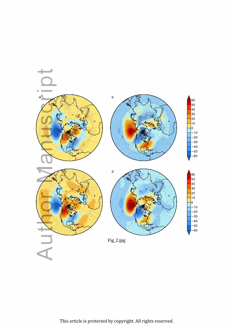
Fig_2.jpg
This article is protected by copyright. All rights reserved.

Fig_3.jpg
This article is protected by copyright. All rights reserved.

Fig_4.jpg
This article is protected by copyright. All rights reserved.