Embed Size (px)
Citation preview

1
Recent Developments in the Application
of Mathematical Programming
to Process Integration
Ignacio E. Grossmann
Center for Advanced Process Decision-making
Department of Chemical Engineering
Carnegie Mellon University
Pittsburgh, PA 15213, U.S.A.
International Process Integration
Jubilee Conference
Gothenburg, Sweden
March 18, 2013

2
Major approaches to Process Integration/Process SynthesisHeuristics (Knowledge Base)
Physical Insights (Pinch Analysis)
Enumerative Search (Means-ends Analysis, Hierarchical Decomposition)
Mathematical Programming (MINLP)
After 30 years, religion war is over!Take best of each approach and combine
Gundersen, T. and I.E. Grossmann, "Improved Optimization Strategies for Automated Heat Exchanger
Networks through Physical Insights," Computers and Chemical Engineering 14, 925 (1990).
Goal: Overview state-of-art and progress of mathematical programming techniques and their application in Process Integration
a) What progress has ben made with mathematical programming tools
(LP, MILP, NLP, MINLP, GDP)?
b) What has been their impact on Process Integration Problems?

3
Math Programming Approach
to Process Synthesis/Integration
1. Develop a superstructure of alternative designs
2. Develop an LP/NLP or (MILP/MINLP, GDP) model to
select topology and parameters of design
3. Solve LP/NLP or (MILP/MINLP, GDP) model to
extract optimum design embedded in superstructure
LP = Linear Programming
NLP = Nonlinear Programming
MILP = Mixed-integer linear programming
MINLP = Mixed-integer nonlinear programming
GBD = Generalized Disjunctive Programming

4
Mathematical Programming
MINLP: Mixed-integer nonlinear programming
mnyRx
yxg
yx hts
yxfZ
1,0,
0,
0),(..
),(min
∈∈
≤
=
=
)(
LP: f, h, g linear, only x
qnmnn RRxgRRxhRRxf →→→ :)(,:)(,:)( 1
NLP: f, h, g nonlinear, only x
MILP: f, h, g linear

5
x1
x2
x1
x2
LP: Linear Programming Kantorovich (1939), Dantzig (1947)
NLP: Nonlinear Programming Karush (1939); Kuhn, A.W.Tucker (1951)
IP: Integer Programming R. E. Gomory (1958)
y1
y2
Evolution of Mathematical Programming

6
- Interior Point Method for LP Karmarkar (1984)
- Convexification of Mixed-Integer Linear ProgramsLovacz & Schrijver (1989), Sherali & Adams (1990),
Balas, Ceria, Cornuejols (1993)
- MINLP Duran & Grossmann (1986)
- Global Optimization Floudas(1990), Sahinidis (1996)
- Logic-based optimization Hooker (1991), Raman & Grossmann (1994)
- Hybrid-systems Barton & Pantelides (1994), Bemporad & Morari (1998)
Major developments in last 30 years
- Modeling Systems GAMS, AMPL, AIMMS
- MILP codes: CPLEX, GUROBI, XPRESS
- NLP codes: MINOS, CONOPT, SNOPT, IPOPT
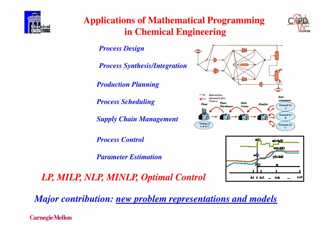
Process Design
Process Synthesis/Integration
Applications of Mathematical Programming
in Chemical Engineering
Plant
WarehousePlant Distr.
CenterRetailer
End
consumers
Material flow
Information flow
(Orders)
Demand for
A
Making of A, B & C
Demand for
B
Demands for C
Plant
WarehousePlant Distr.
CenterRetailer
End
consumers
Material flow
Information flow
(Orders)
Demand for
A
Demand for
A
Making of A, B & C
Demand for
B
Demand for
B
Demands for C
Demands for C
t-1 t+1 t+kt ......
N
u(t+k|t)
y(t+k|t)
w(t+k|t)
t-1 t+1 t+kt ......
N
u(t+k|t)
y(t+k|t)
w(t+k|t)
t-1 t+1 t+kt ......
N
u(t+k|t)
y(t+k|t)
w(t+k|t)
t-1 t+1 t+kt ......
N
u(t+k|t)
y(t+k|t)
w(t+k|t)
t-1 t+1 t+kt ......
N
u(t+k|t)
y(t+k|t)
w(t+k|t)
t-1 t+1 t+kt ......
N
u(t)
w(t)
u(t+k|t)
y(t+k|t)
y(t)
w(t+k|t)
t-1 t+1 t+kt ......
N
u(t+k|t)
y(t+k|t)
w(t+k|t)
t-1 t+1 t+kt ......
N
u(t+k|t)
y(t+k|t)
w(t+k|t)
t-1 t+1 t+kt ......
N
u(t+k|t)
y(t+k|t)
w(t+k|t)
t-1 t+1 t+kt ......
N
u(t+k|t)
y(t+k|t)
w(t+k|t)
t-1 t+1 t+kt ......
N
u(t+k|t)
y(t+k|t)
w(t+k|t)
t-1 t+1 t+kt ......
N
u(t)
w(t)
u(t+k|t)
y(t+k|t)
y(t)
w(t+k|t)
t+Nt-1 t+1 t+kt ......
N
u(t+k|t)
y(t+k|t)
w(t+k|t)
t-1 t+1 t+kt ......
N
u(t+k|t)
y(t+k|t)
w(t+k|t)
t-1 t+1 t+kt ......
N
u(t+k|t)
y(t+k|t)
w(t+k|t)
t-1 t+1 t+kt ......
N
u(t+k|t)
y(t+k|t)
w(t+k|t)
t-1 t+1 t+kt ......
N
u(t+k|t)
y(t+k|t)
w(t+k|t)
t-1 t+1 t+kt ......
N
u(t)
w(t)
u(t+k|t)
y(t+k|t)
y(t)
w(t+k|t)
t-1 t+1 t+kt ......
N
u(t+k|t)
y(t+k|t)
w(t+k|t)
t-1 t+1 t+kt ......
N
u(t+k|t)
y(t+k|t)
w(t+k|t)
t-1 t+1 t+kt ......
N
u(t+k|t)
y(t+k|t)
w(t+k|t)
t-1 t+1 t+kt ......
N
u(t+k|t)
y(t+k|t)
w(t+k|t)
t-1 t+1 t+kt ......
N
u(t+k|t)
y(t+k|t)
w(t+k|t)
t-1 t+1 t+kt ......
N
u(t)
w(t)
u(t+k|t)
y(t+k|t)
y(t)
w(t+k|t)
t+NLP, MILP, NLP, MINLP, Optimal Control
Production Planning
Process Scheduling
Supply Chain Management
Process Control
Parameter Estimation
Major contribution: new problem representations and models

8
Progress in Mixed-Integer Linear Programming
Unit-Commitment Model: California 7-Day Model
2,856 0-1 vars, 22,899 cont vars, 48,939 constr.
1999 CPLEX 7.0: 1 hr initial LP, unfinished after 8 hours
2010 Gurobi 3.0: ~3 min (195 secs) to optimality!
=> 80,000 speed-up!!
Bixby, Rothberg and Gu (2011)
CPLEX 1.2 to Gurobi 3.0
on same computer

9

NLP: Algorithms (variants of Newton's method)
Sucessive quadratic programming (SQP) (Han 1976; Powell, 1977)
Reduced gradient Interior Point Methods
Major codes: MINOS (Murtagh, Saunders, 1978, 1982)
CONOPT (Drud, 1994)
SQP: SNOPT (Murray, 1996) OPT (Biegler, 1998) KNITRO (Nocedal, 2000) IP: IPOPT (Wächter, Biegler, 2002) www.coin-or.org Typical sizes: 100,000 vars, 100,000 constr. (unstructured) 1,000,000 vars (few degrees freedom) Convergence: Good initial guess essential (Newton's) Nonconvexities: Local optima, non-convergence
Nonlinear Programming
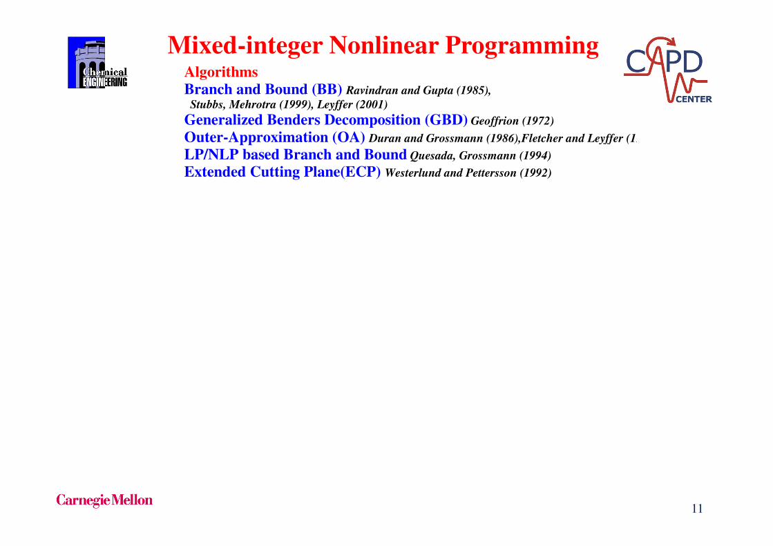
11
Algorithms Branch and Bound (BB) Ravindran and Gupta (1985),
Stubbs, Mehrotra (1999), Leyffer (2001) Generalized Benders Decomposition (GBD) Geoffrion (1972)
Outer-Approximation (OA) Duran and Grossmann (1986),Fletcher and Leyffer (1994)
LP/NLP based Branch and Bound Quesada, Grossmann (1994)
Extended Cutting Plane(ECP) Westerlund and Pettersson (1992)
Availability of New Codes: SBB GAMS simple B&B
MINLP-BB (AMPL)Fletcher and Leyffer (1999)
Bonmin (COIN-OR) Bonami et al (2006) FilMINT Linderoth and Leyffer (2006)
KNITRO Nocedal (2009)
DICOPT (GAMS) Viswanathan and Grossman (1990)
AOA (AIMSS)
α−α−α−α−ECP Westerlund and Peterssson (1996) MINOPT Schweiger and Floudas (1998)
BARON Sahinidis et al. (1998)
Couenne Belotti, Margot (2008)
Mixed-integer Nonlinear Programming
Typical sizes: up to 1000 0-1 variables, 10,000 cont. vars./constraints

12

13
(((( ))))
Ω
,0)(
0)(
)(min
1
falsetrue,Y
Rc,Rx
trueY
K k
γc
xg
Y
Jj
xs.t. r
xfc Z
jk
k
n
jkk
jk
jk
k
kk
∈∈∈∈
∈∈∈∈∈∈∈∈
====
∈∈∈∈
====
≤≤≤≤∈∈∈∈
≤≤≤≤
∑∑∑∑ ++++====
∨∨∨∨
Raman and Grossmann (1994) (Extension Balas, 1979)
Motivation: Facilitate modeling discrete/continuous problems
Codes: LOGMIP, EMP
Objective Function
Common Constraints
Continuous Variables
Boolean Variables
Logic Propositions
OR operator
Disjunction
Fixed Charges
Constraints
Generalized Disjunctive Programming (GDP)

14
Global Optimization Algorithms
Algorithms based on spatial branch and bound method
and use of underestimators/convex envelopes (Horst & Tuy, 1996)
•Nonconvex NLP/MINLP
ααααBB (Adjiman, Androulakis & Floudas, 1997; 2000)
BARON (Branch and Reduce) (Ryoo & Sahinidis, 1995,
Tawarmalani and Sahinidis, 2002)
Branch and cut (Kesavan, Allgor, Gatzke and Barton, 2004)
Branch and Contract (Zamora & Grossmann, 1999)
Transformation signomials (Bjoerk, Lindberg, Westerlund, 2002)
Couenne (COIN-OR) (Belotti & Margot, 2008)
•Nonconvex GDP
Two-level Branch and Bound (Lee & Grossmann, 2001)
Bound strengthening (Ruiz, Grossmann, 2010)
Typical sizes: up to 100 0-1 variables, 1,000 cont. vars./constraints

15
http://www.minlp.org

16
Synthesis of Heat Exchanger NetworksYee and Grossmann (1990)
H1
H1-C1
H2
H1-C1
H1-C2
H2-C1
H2-C2
H1-C2
H2-C1
H2-C2
Stage k=1 Stage k=2
C1
C2
temperature
location
k=1
temperature
location
k=2
temperature
location
k=3
H1,1t
H1,2t
C1,1tC1,2t
C1,3t
H1,3t
H2,1t
H2,2tC2,1t C2,2t
C2,3t
H2,3t
S1
S1
CW
CW
Multiple stages with potential heat exchangers zijk = 0,1
3 hot, 4 cold streams
MINLP 67 0-1, 270 cont vars, 258 constr. 3s CPU-time (DICOPT-2013)

17
18
1
2
3
4
5
6
H1
H2
H3
H4
C2
C1
QFuel
R1
R2
R3
R4
R5
QLP
QHP
2000
1800
1000
800
3600
2000
2000
3500
2000
2000
3500
3500
4700
9000
9000
2500
2500
2500
4500
3000
14500
18000
QCW
4700
10500
11600
5600
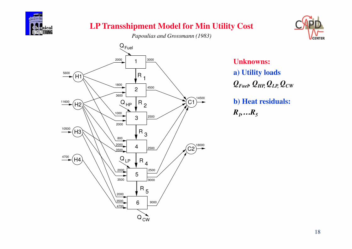
LP Transshipment Model for Min Utility CostPapoulias and Grossmann (1983)
Unknowns:
a) Utility loads
QFuel, QHP, QLP, QCW
b) Heat residuals:
R1,…R5

Transshipment Model
19
Case Study Results for Similar Fcps (Academic)
Problem Size LP Transshipment Model MILP Transshipment Model
# of Hot Streams *
# of Cold Stream
# of
Variables
# of
Constraints
CPU
Time
(seconds)
# of
Continuous
Variables
# of Binary
Variables
# of
Constraints
Optimum
Solution /
Best
Bound
LP
Relaxation
CPU Time
(seconds)
2 * 2 38 22 0.031 38 10 32 8 7 0.156
3 * 3 72 37 0.031 72 17 54 8 6.179 0.047
5 * 5 235 89 0.031 235 67 156 24 16.302 0.421
10 * 10 1057 256 0.031 1057 219 475 42 28.848 1059.309
15 * 15 2692 506 0.031 2692 421 927 57 40.149 3600*
20 * 20 6284 902 0.031 6284 778 1680 83 56.868 3600*
* Time limit
Chen, Miller, Grossmann (2013)

20
Problem Size LP Transshipment Model MILP Transshipment Model
# of Hot Streams
# of Cold Stream
# of
Variables
# of
Constraints
CPU
Time
(seconds)
# of
Continuous
Variables
# of Binary
Variables
# of
Constraints
Optimum
Solution /
Best
Bound
LP
Relaxation
CPU Time
(seconds)
2 * 2 38 22 0.047 38 12 34 9 7.650 0.187
3 * 3 72 37 0.031 72 24 61 14 11.624 0.189
5 * 5 235 89 0.031 235 67 156 26 17.931 0.311
10 * 10 1057 256 0.047 1057 196 452 39 29.194 23.104
15 * 15 2692 506 0.016 2692 392 898 55 41.258 760.583
20 * 20 6284 902 0.031 6284 712 1614 81 56.469 3600*
Transshipment Model
Case Study Results for Dissimilar Fcps (Industrial)
* Time limit
MILP Industrial Problems Easier to Solve!

21
Carnegie Mellon
Superstructure of the integrated water network
MINLP: 72 0-1 vars, 233 cont var, 251 constr
optcr=0.01 197.5 CPUsec (BARON)

22
Carnegie Mellon
Optimal design of the simplified water network
with 13 removable connections
Optimal Freshwater
Consumption
40 t/h
vs
300 t/h conventional
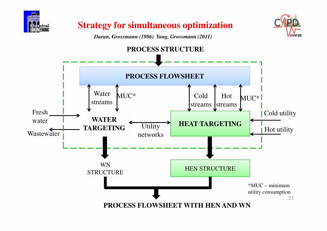
HEAT TARGETING
PROCESS FLOWSHEET
WATER
TARGETING
Cold
streams
Hot
streamsMUC*
*MUC – minimum
utility consumption
Hot utility
Cold utility
MUC*Water
streams
Wastewater
Fresh
waterUtility
networks
PROCESS STRUCTURE
WN
STRUCTUREHEN STRUCTURE
PROCESS FLOWSHEET WITH HEN AND WN23
Strategy for simultaneous optimizationDuran, Grossmann (1986) Yang, Grossmann (2011)

24
Carnegie Mellon
outin
k
j
pkp
j
i
j
piin
p
out
i
out
p
in
k
inout
i
j
k
j
in
si
ik
out
mi
iU
ji
kU
jk
out
mi
ik
pkpiPUpj
CGainFLCLossF
piPUpPF
pkPUpPF
sksiSUsjCC
skSUsFF
mkMUmjCFCF
mkMUmFF
out
in
in
∈∈∈∀∀
−=+−
∈∈∀=
∈∈∀=
∈∈∀∈∀∀=
∈∈∀=
∈∈∀∀≥
∈∈∀=
∑
∑
∑
∈
∈
∈
,,,
)()(
,
,
,,
,
,,
,s.t.
,
fwFZ =min
Splitters mass
balances
Process
unit mass
balances
Mixer mass
balances
LP Targeting model for minimum freshwater consumption
Assumes only process units (reuse, recycle)
Yang, Grossmann (2012)

25
Carnegie Mellon
SEQUENTIAL SIMULTANEOUS
Profit (1000 $/yr) 62,695 73,416
Investment cost (1000 $) 1,891 1,174
Operating parameters
electricity (KW) 6.59 1.84
freshwater (kg/s) 36.43 29.25
heating utility (109 KJ/yr) 0.293 0
cooling utility (109 KJ/yr) 67.3 72.7
Steam generated (109 kJ/yr) 2448 1965
overall conversion 0.68 0.88
Material flowrate (106 kmol/yr)
feedstock 48.04 37.13
product 10.89 10.89
Sequential vs. simultaneous result comparison
Methanol Process
from Syngas
17%
improvement
17%
improvement
LP exact target!LP exact target!

2626
Optimization of Number of Trays
Discrete variables: Number of trays, feed tray location.
Continuous variables: reflux ratio, heat loads, exchanger areas, column diameter.
No liquid on tray
No vapor on tray
Existing trays
Vapor Flow
Liquid Flow
Viswanathan & Grossmann (1993)
Non-existing tray
Non-existing tray
1=mzr
1=nzb
1,0=izb
MINLP =>
1,0=izr
Acetone-acetonitrile-water, max 25 trays, Virial-UNIQUAC
MINLP: 22 0-1 vars, 891 cont, vars, 957 const.
Number
trays
40 minutes in 1992, 10 secs in 2013!!

27
Problem Specs
Mixture: Methanol/ Ethanol/ Water
Feed composition: 0.5/ 0.3/ 0.2
Feed: 10 moles/s
Pressure: 1 atm
Max no. trays: 20 (per section)
Min purity: 95%
Ideal/Wilson models
F
methanol
ehtanol
Azeotrope
Water
ethanol
Superstructure
0.0 0.1 0.2 0.3 0.4 0.5 0.6 0.7 0.8 0.9 1.00.00.10.20.30.40.50.60.70.80.91.0Mole Fraction Methanol
Mole Fraction Ethanol
Feed Liq. Col. 1 Liq. Col. 2 Liq. Col. 3 Liq. Col. 4 Liq. Col. 5Initialization
GDP Model
Discrete Variables 210
Continuous Variables 9025
Constraints 8996
Bartfeld, Aguirre, Grossmann (2004)
Azeotropic Example

28
Product Specifications 95%
Optimal Configuration $318,400 /yr
Optimal Solution
Annual Cost ($/year) 318,400
Preprocessing (min) 6.05
Subproblems NLP (min) 36.3
Subproblems MILP (min) 3.70
Iterations 3
Total Solution Time (min) 46.01
667MHz. Pentium III PC
0.0 0.1 0.2 0.3 0.4 0.5 0.6 0.7 0.8 0.9 1.00.00.10.20.30.40.50.60.70.80.91.0
Mol
e Fr
actio
n M
etha
nol
Mole Fraction Ethanol
Fedd Liq. Col 1 Liq. Col 2 Liq. Col 3Profiles Optimal Configuration
F
PP6 = 1.292 mole/sec
95% Water
PP1 = 5.158 mole/sec
95% Methanol
PP4 = 0.836 mole/sec
95% Ethanol
39
38
35
PP5 = 2.376 mole/sec
Azeotrope
622 kW
260 kW
200 kW
4 out of 10 sections deleted
Azeotropic Example

29
A/BCDEFGH
ABCDEFGH
STATES TASKS
AB/CDEFGH
ABCD/CDEFGH
ABCDEF/CDEFGH
ABCDEF/EFGH
ABCD/EFGH
ABCDEF/GH
ABCDEFG/H
ABCDEFG
BCDEFGH
NON-SHARP
A/BCDEFG
AB/CDEFG
ABCD/CDEFG
ABCDEF/CDEFG
ABCDEF/EFG
ABCD/EFG
ABCDEF/G
B/CDEFGH
BCD/EFGH
BCD/CDEFGH
BCDEF/CDEFGH
BCDEF/EFGH
BCDEF/GH
BCDEFG/H
ABCDEF
BCDEFG
CDEFGH
A/BCDEF
AB/CDEF
ABCD/CDEF
ABCD/EF
BCDEF/G
B/CDEFG
BCD/CDEFG
BCDEF/CDEFG
BCDEF/EFG
BCD/EFG
CDEFG/H
CD/EFGH
CDEF/EFGH
CDEF/GH
BCDEF
CDEFG
ABCD
AB
BCD
EFG
CDEF
EFGH
GH
EF
CD
A
B
C
D
F
E
G
H
CD/EFG
CDEF/EFG
CDEF/G
B/CDEF
BCD/CDEF
BCD/EF
A/BCD
AB/CD
CD/EF
EF/GH
EFG/H
B/CD
EF/G
G/H
E/F
C/D
A/B
H2
CH4
C2H4
C3H6
C2H6
C3H8
C4
C5
25 states
53 separation tasks
Feed
GDP→→→→big-M MINLP: 5,800 0-1 vars, 24,500 cont. vars., 52,700 constraints ~3hrs CPU-time
Superstructure Separations Olefins Plant(Lee, Foral, Logsdon, Grossmann, 2003)
A- H2
B- CH4
C- C2H4
D- C2H6
E- C3H6
F- C3H8
G- C4
H- C5

30
Total cost: 110.82 MM$/yr
ABCDEFGH
AB
CDEFGH
EF
CD
B
A
D
C
E
F
H
G
A/B
CH4
C2H4
C3H6
C2H6
C3H8
C4
C5
H2
EFGH
Cold Box
Deethanizer
Dephlegmator
100F
480Psig
83F
160Psig
-141F
900Psig
-41F
160Psig
84F
190Psig
169F
160Psig
D
E
E
F
C
D
123F
140Psig
99F
140Psig
GH
G
H
Depropanizer
C3Splitter
226F
160Psig
compressor
heater
cooler
valve
480Psig
74F
170Psig
72F
140Psig
480Psig
-31F
140Psig
-51F
140Psig
214F
170Psig
109F
140Psig
F
G
Debutanizer
236F
140Psig
238F
140Psig
AB
CD
900Psig
Chemical Absorber
410 Mkwh/yr
valve
compressor
pump
pump
MINLP optimal solution
Dephlegmator first process
7 separation units
1 dephlegmator
1 absorber
4 distillation columns
1 cold box
1 heat exchange
20M$/yr cost saving

31
Power
Grid
CHP plantTypically multiple boilers and
turbines (steam, gas)
Chemical
plant
Fuel
Electricity
Steam at
different
pressure
levels
Raw
materials
Products
Use the flexibility
of the CHP plant to
adjust steam production
for variability
in electricity price
Electricity prices
vary on an
hourly basis
Account for
variability in
electricity prices
in production
planning1
The incentives given by utilities and grid operators to adjust power consumption/
production increase profitability, if the processes are able to cope with variability2.
HRSG
B
1
B
3
ST1 ST2B2
GT~
X
I
II
1. Mitra, S., I.E. Grossmann, J.M. Pinto and Nikhil Arora, "Optimal Production Planning under Time-sensitive Electricity Prices for
Continuous Power-intensive Processes”, Computers & Chem. Eng., 2012, 38, 171-184
2. Samad, T.; Kiliccote, S., “Smart Grid Technologies and Applications for the Industrial Sector”, Computers & Chem. Eng., 2012.
Wassick, J.M., Enterprise-wide optimization in an integrated chemical complex, Computers & Chem. Eng., 2009, 33, 1950–1963
Optimal Scheduling of Industrial Combined Heat
and Power Plants under Time-sensitive Electricity Prices
Mitra, Sun, Grossmann (2012)Demand Side Management
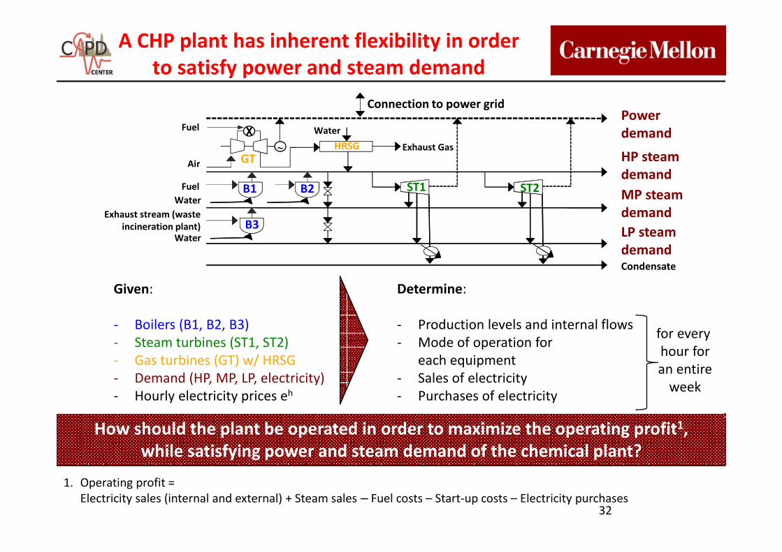
A CHP plant has inherent flexibility in order
to satisfy power and steam demand
32
Given:
- Boilers (B1, B2, B3)
- Steam turbines (ST1, ST2)
- Gas turbines (GT) w/ HRSG
- Demand (HP, MP, LP, electricity)
- Hourly electricity prices eh
Determine:
- Production levels and internal flows
- Mode of operation for
each equipment
- Sales of electricity
- Purchases of electricity
for every
hour for
an entire
week
1. Operating profit =
Electricity sales (internal and external) + Steam sales – Fuel costs – Start-up costs – Electricity purchases
MP steam
demand
LP steam
demand
HP steam
demand
Power
demand
Condensate
Exhaust stream (waste
incineration plant)
HRSG
Connection to power grid
B1
B3
ST1 ST2B2Water
Fuel
Water
Exhaust Gas
Water
GT
Fuel
~
Air
X
How should the plant be operated in order to maximize the operating profit1,
while satisfying power and steam demand of the chemical plant?

Disjunctive Programming (DP) is used as a
modeling framework to represent the CHP plant
33
Disjunction over operating modes to describe feasible region of operation2
- How to represent each component in terms of
state graph and feasible region?
Mass balances, demand constraints and additional constraints
(e.g. energy exchange with the grid, restrictions on shutdowns)
max Electricity sales (internal and external) + Steam sales
– Fuel costs – Start-up costs – Electricity purchases
Objective function:
Maximize operating profit over an entire week (7*24 hours = 168 discrete time periods)
for each
CHP plant
component
Logic constraints to model restrictions of the state graph
- How to address the previously mentioned model requirements?
Ramping constraints
1
2
3
The model has 70,009 constraints, 49,535 variables
(8,722 binaries) and can be solved within 2 minutes (CPLEX 12.4)

Weekly profiles for a case with 61% utilization1
and 2 shutdowns allowed per component
34
Steam profiles
for boilers
and gas turbine
Electricity profiles
for steam
and gas turbines
HP steam input
profiles for
steam turbines
MP, LP and
cond. output
profiles for
steam turbines
Electricity price
profile
1. Capacity utilization as percentage of maximum steam production.

35
Conclusions
1. Discrete/continuous optimization methods have had- tremendous progress in MILP
- very significant progress in MINLP/GDP
- good progress in global MINLP/GDP
3. Math Programming models used increasingly by industry
2. Mathematical Programming has significantly impacted
Process Integration- Heat Exchanger Networks
- Water Networks
- Power Systems
- Separation Systems
- Process Flowsheets
Math Programming can be successfully used in combination
with heuristics, physical insights, enumerative methods