RECOMMENDATION ITU-R S.2029 - Statistical methodology to assess

Recommendation ITU-R S.2029(12/2012)

Statistical methodology to assess time-varying interference produced by

a geostationary fixed-satellite service network of earth stations operating with

MF-TDMA schemes to geostationaryfixed-satellite service networks

S SeriesFixed-satellite service

ii Rec. ITU-R S.2029

Foreword

The role of the Radiocommunication Sector is to ensure the rational, equitable, efficient and economical use of the radio-frequency spectrum by all radiocommunication services, including satellite services, and carry out studies without limit of frequency range on the basis of which Recommendations are adopted.

The regulatory and policy functions of the Radiocommunication Sector are performed by World and Regional Radiocommunication Conferences and Radiocommunication Assemblies supported by Study Groups.

Policy on Intellectual Property Right (IPR)

ITU-R policy on IPR is described in the Common Patent Policy for ITU-T/ITU-R/ISO/IEC referenced in Annex 1 of Resolution ITU-R 1. Forms to be used for the submission of patent statements and licensing declarations by patent holders are available from http://www.itu.int/ITU-R/go/patents/en where the Guidelines for Implementation of the Common Patent Policy for ITU-T/ITU-R/ISO/IEC and the ITU-R patent information database can also be found.

Series of ITU-R Recommendations

(Also available online at http://www.itu.int/publ/R-REC/en)

Series Title

BO Satellite delivery

BR Recording for production, archival and play-out; film for television

BS Broadcasting service (sound)

BT Broadcasting service (television)

F Fixed service

M Mobile, radiodetermination, amateur and related satellite services

P Radiowave propagation

RA Radio astronomy

RS Remote sensing systems

S Fixed-satellite service

SA Space applications and meteorology

SF Frequency sharing and coordination between fixed-satellite and fixed service systems

SM Spectrum management

SNG Satellite news gathering

TF Time signals and frequency standards emissions

V Vocabulary and related subjects

Note: This ITU-R Recommendation was approved in English under the procedure detailed in Resolution ITU-R 1.

Electronic Publication Geneva, 2012

ITU 2012

All rights reserved. No part of this publication may be reproduced, by any means whatsoever, without written permission of ITU.

http://www.itu.int/ITU-R/go/patents/en

http://www.itu.int/publ/R-REC/en

Rec. ITU-R S.2029 1

RECOMMENDATION ITU-R S.2029

Statistical methodology to assess time-varying interference produced by a geostationary fixed-satellite service network of earth stations

operating with MF-TDMA schemes to geostationary fixed-satellite service networks

(Question ITU-R 208/4)

(2012)

Scope

This Recommendation provides a statistical methodology to assess time-varying interference resulting from a geostationary network of earth stations, operating with MF-TDMA schemes, over a geostationary-satellite orbit fixed-satellite service network. The methodology considers the potential interference to another GSO FSS network. Furthermore, the methodology can be used to adjust the power levels of the interfering terminals such that the performance objectives of the interfered-with satellite network are not impacted.

The ITU Radiocommunication Assembly,

considering

a) that FSS GSO satellites are well suited to provide broadband communication applications including Internet and data services;

b) that satellite networks use a variety of network topologies and multiple access schemes, including the multi-frequency time division multiple access (MF-TDMA) scheme;

c) that through the use of efficient modulation and coding, higher satellite e.i.r.p. levels, and other techniques, some networks can support full mesh (point-to-point) connectivity with small aperture terminals;

d) that it is necessary to protect networks of the FSS from any potential interference from these terminals;

e) that it would be useful to have methodologies to assess the time-varying interference from a GSO FSS network to another GSO FSS network;

f) that it would be useful to have methodologies for assessing interference levels to satellite networks resulting from earth stations operating with MF-TDMA schemes;

g) that many of the technical characteristics of these networks which affect performance and orbit spectrum/utilization have time-varying characteristics which are best modelled by stochastic processes,

noting

a) that maximum permissible levels of inter-network interference from GSO networks to GSO/FSS networks operating in the same frequency band are provided in Recommendation ITU-R S.1323;

b) that maximum permissible levels of inter-network interference and the methodology for determining this interference, from non-GSO systems and to GSO/FSS networks operating in the same frequency band are provided in Recommendation ITU-R S.1323;

c) that time invariant interference is typically estimated using the ΔT /T method, described in Recommendation ITU-R S.738;

2 Rec. ITU-R S.2029

d) that methodologies to estimate the off-axis e.i.r.p. density levels and to assess the time-varying interference towards adjacent satellites resulting from pointing errors of a vehicle mounted earth station are provided in Recommendation ITU-R S.1857,

recommends

1 that the methodology given in the Annex should be used to assess the time-varying interference due to multiple earth stations operating in a MF-TDMA scheme;

2 that the methodology provided should be used to determine the off-axis emission levels of the interfering earth stations such that these satisfy the performance objectives of the interfered-with satellite network;

3 that the methodology provided should be used so that the type of MF-TDMA networks described in this Recommendation would not create interference to other FSS networks operating in the same frequency bands beyond the level accepted by administrations;

4 that the following Notes should be regarded as part of this Recommendation.

NOTE 1 – The methodology given in the Annex provides a statistical approach to assess the potential interference impacts of an MF-TDMA network to a neighbouring co-frequency GSO FSS network.

NOTE 2 − The parameters and the examples provided in the Annex represent a hypothetical system that operates in the 20/30 GHz frequency band. However, the methodology may also be used for other frequency bands after appropriate modifications of some parameters.

NOTE 3 – The methodology of this Recommendation does not apply to networks operating with code division multiple access (CDMA) schemes.

NOTE 4 – To verify that the mathematical model described in the methodology truly represents the time-varying characteristics of an MF-TDMA network, it may be useful to obtain the statistical characteristics of operational networks.

NOTE 5 – The apportionment of short-term interference for the MF-TDMA GSO/FSS networks considered in this Recommendation may be mutually agreed through the process of coordination.

NOTE 6 – The time allowance and the short-term interference criteria for GSO/FSS networks may be a subject for further study.

Annex

Statistical methodology to assess time-varying interference produced by a geostationary fixed-satellite service network of earth stations

operating with MF-TDMA schemes to geostationary fixed-satellite service networks

1 Introduction

In recent years, the demand for satellite-based two-way Internet services has increased significantly. These services, especially for residential and small business users, are provided using small aperture satellite terminals. Typically, a single satellite network may consist of a large number of small aperture terminals deployed over a wide geographical area. According to the location within the

Rec. ITU-R S.2029 3

satellite footprint, the varying weather conditions, and the user’s data rates, these terminals may operate on a range of aperture sizes and may require different transmit power levels. To utilize network resources efficiently, these networks may employ time- and frequency-division multiple access methods. A particular characteristic of small aperture terminals is that they have large antenna beamwidths and hence may produce uplink interference towards adjacent satellites if the transmit power levels are not adjusted properly. Additionally, some small terminals mounted on air/sea vessels, trains, or ground vehicles as well as stationary terminals may produce antenna pointing errors which may result in potential interference that must be mitigated. These combined effects contribute to a time-varying interference pattern from the network of terminals to a victim receiver in another satellite network.

This Annex presents a statistical approach to determine the interference to a GSO network from another GSO network consisting of multiple terminals operating using a time-division multiple access scheme and antenna pointing errors. The Annex discusses a long-term interference criterion and criteria to satisfy the short-term performance objectives, it provides some examples to illustrate the impacts on the neighbouring satellite network, and it presents a step-by-step approach on how to compute the resulting interference. The methodology presented may be useful to determine the off-axis emission levels of the interfering terminals such that these satisfy the short-term and long-term performance objectives of the victim satellite system.

2 Long- and short-term components of interference

The interference signal at the victim receiver consists of signals that belong to a large number of transmit terminals from a single interfering network that operate using a time-division multiple access protocol. The terminals may employ antenna apertures of different sizes and may transmit at different power levels depending on their location within the footprint of the satellite beam. Additionally, these terminals may have small antenna pointing errors. Therefore, when the observation interval is sufficiently large to contain transmissions from several interfering terminals, the interference level at the victim receiver is time-varying.

In such cases, for illustrative purposes, the interference signal at the victim receiver, , may be expressed as the sum of a long-term interference component, , and a short-term interference component, , so that = + . The long-term interference component is constant over short time intervals but it may exhibit small variations when observed over long time intervals (of the order of several minutes). These variations are statistical in nature resulting from the slow changing characteristics of the transmit signals. On the other hand, the short-term interference component is due to the transmissions from different terminal types and may vary over very short time intervals, for example over fractions of a second. Note that this short-term and long-term interference components are used only for illustrative purposes; interference analysis is carried out for the total interference.

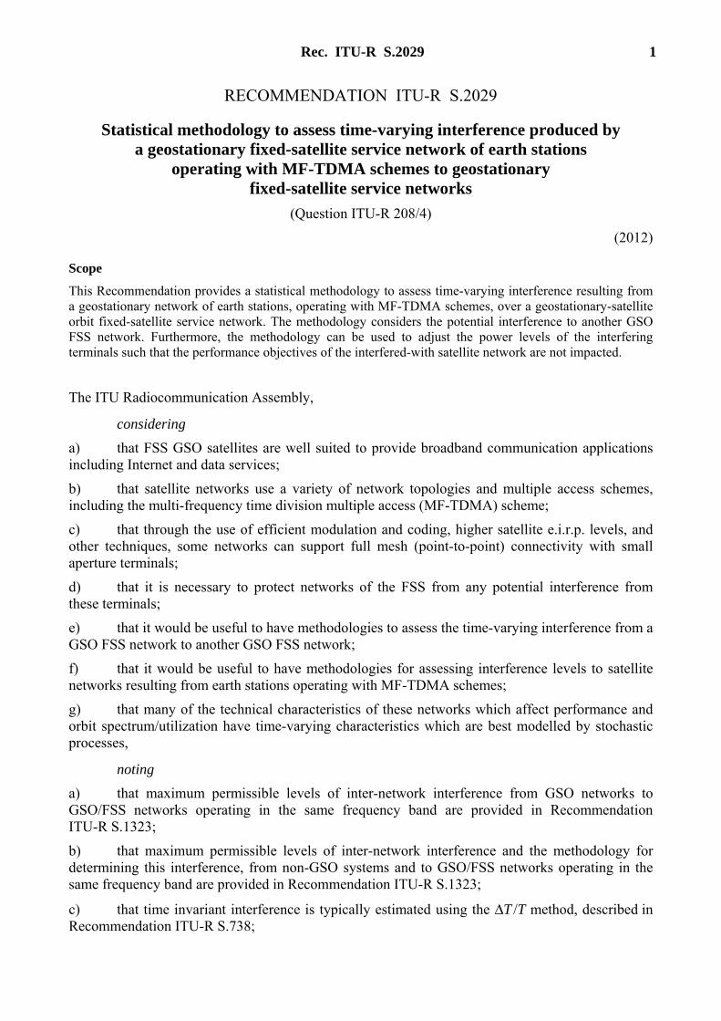
Figure 1 shows the interference levels at the victim receiver due to transmissions from Terminals T1, T2, T3, T4 and T5. In general, as shown in this figure, the interference levels and the transmission durations depend on the particular terminal. The long-term component shown here represents the average level of the interference and the short-term interference component is given by the difference between the total interference and this long-term interference component.

To quantify and limit the effects of interference, this Annex gives methods for assessing and limiting the long-term interference, short-term interference, and total interference. Specifically, long-term interference and the criteria to satisfy the short-term performance objectives are given to limit the effects of interference at the victim receiver.

4 Rec. ITU-R S.2029

FIGURE 1

Interference observed at the victim receiver due to time-division multiple access transmissions from Terminals T1, T2, T3, T4 and T5

S.2029-01

Interference signal at victim receiver

I – totalinterferencetot

T1 T2 T3 T2 T4 T5T1

I – long-termcomponentlong

Time

3 Long-term interference criterion

Assessment of time invariant interference is typically carried out using the ΔT/T method, for example as described in Recommendation ITU-R S.738. In order to make use of a similar approach consider the hypothetical situation when the interference level at the victim receiver is not time-varying: that is the e.i.r.p. density levels at the terminals are adjusted so that the interference level seen at the victim receiver is given by long-term interference level, . Also, in this case the terminals do not produce antenna pointing errors. The long-term interference criterion in this case is expressed in terms of the ΔT/T ratio as:

svvv

long

long

kI

T

T

Θγ+Θ=

Δ /

~ (1)

where is defined as the ensemble-averaged interference power spectral density computed in a bandwidth of , k is the Boltzmann constant, Θ is the victim receiver noise temperature referred to the output of its antenna, Θ is the noise temperature at the receiver of the victim satellite referred to the output of its antenna, and γ is the transmission gain from the output of the victim satellite’s input antenna to the output of the victim receiver’s antenna.

Clearly, when the ensemble-averaged power of the interference is a constant, the interference power-to-noise ratio considered in this hypothetical case is time invariant.

However, in practice, rather than the ensemble-average value the time-averaged value of the long-term interference component is generally available. This time average value may exhibit small variations when computed over different time intervals. This time-averaged value, , when computed over the long-term time interval of duration may exhibit variations because the underlying interference is a statistical process. Additionally, statistical characteristics of the terminals may change during this interval resulting in small variations about this average value. These variations can be limited by imposing constraints on the cumulative distribution function (CDF) of the variable ( )longTT /Δ as follows:

Pr

ΔT

T

long

> X%

< plong%

(2)

where X , plong and are system parameters.

For illustrative purposes, Recommendation ITU-R S.523-4 specifies an averaging interval of 10 min for computing the interference to PCM encoded Telephony systems. Moreover, Annex 1 of Recommendation ITU-R S.1432-1 specifies the maximum levels of interference-to-noise ratio (I / N) that may be exceeded in any month as: (I / N) > 0 dB for 0.005% of any month;

Rec. ITU-R S.2029 5

(I / N) > −2.4 dB for 0.03% of any month; (I / N) > −10 dB for 20% of any month; and (I / N) > −12 dB for 100% of any month.

4 Criteria to satisfy short-term performance objectives

In the preceding section, limits were imposed on the long-term interference. In this section, a criterion is presented to limit the total interference so that it meets the short-term performance objectives of the victim receiver. The total interference may exhibit variations over a few milliseconds. According to Recommendation ITU-R S.1323-2, victim links should contain sufficient link margins to overcome degradations due to the combined effects of propagation and time-varying interference. Degradations due to propagation effects should not account for more than 90% of the time allocated in the short-term performance objectives. Additionally, this Recommendation states that time-varying interference “should be responsible for at most 10% of the time allowance for the BER (or C/N value) specified in the short-term performance objectives of the desired network and corresponding to the shortest percentage of time (lowest C/N value).” In this Annex, a criterion similar to the above is presented to derive an acceptable limit for the short-term interference.

The short-term performance objectives are usually stated in terms of the bit-error-rate (BER) levels or the carrier-to-noise (C/N) ratio levels that may not be degraded for a specified time period. For example, for a given C/N ratio and time percentage pairs, ( / ) , % , = 1,2, … , ,the C/N ratio may be less than( / ) for only % of the time of any month. Similar to considering o) in Recommendation ITU-R S.1323-2, let us consider propagation effects to result in degradation of the link for at most (1 − /100) × %, = 1,2, … , , of the time of any month where represents the fraction of the time allowance specified in the short-term performance objective allocated to short-term interference (for example, = 10). Noting that the long-term interference is limited as proposed in the previous section, the proposed criteria to limit the short-term interference and comply with the short-term performance objectives are expressed as:

a) In the presence of propagation effects and the long-term interference, the C/N ratio should not be less than( / ) for more than (1 − /100) × %, = 1,2, … , , (for example, = 10)of the time of any month.

b) In the presence of short-term interference, the C/N ratio should not be less than( / ) for more than ( /100) × %of the time of any month, where j corresponds to the smallest ( / ) value.

c) In the presence of propagation effects and total interference, the C/N ratio should not be less than ( / ) for more than %, = 1,2, … , , of the time of any month.

Note that in order to comply with the above conditions, the victim link should contain a sufficient link margin to satisfy condition a) and the e.i.r.p. density level of the interferer should be limited to satisfy conditions b) and c). Also note that according to condition c), the combined impact of propagation degradation and the total interference is such that C/N ratio still meets the short-term performance objective.

4.1 Expressing the C/N ratios

The C/N ratio under clear-sky conditions, considering the long-term interference component can be expressed as:

( )longCS

CSCS IN

CNC

+=/

6 Rec. ITU-R S.2029

where is the carrier power under clear-sky conditions, noise power at the victim receiver under clear-sky conditions and is the long-term interference power component under clear-sky conditions.

Next, consider the C/N ratio under rain fading conditions. The rain attenuation factors in the uplink and downlink of the victim signal link are denoted by ↑ and ↓, respectively. The carrier power at the victim receiver under these conditions will be attenuated by the factor ( ↑, ↓) and is denoted by ( ↑, ↓). The noise power at the receiver is denoted by the function ( , ↓). This function includes the sky noise due to rain and the noise components from the wanted and adjacent satellites. Note that the attenuation factors due to rain in the downlink from adjacent satellites may not be the same as ↓. In such cases this noise function should take into account these different rain attenuation factors. Under rain fading conditions the long-term interference component is denoted by , ↓, ↑, where ↑, is the uplink rain attenuation factor from the interfering terminal to the wanted satellite. Note that when the uplink rain attenuation factors are not the same for the different interfering terminals, these different rain attenuation factors should be considered in this expression. Moreover, when the downlink rain attenuation components from the adjacent and wanted satellites are not the same, the different downlink rain attenuation factors from the adjacent satellites should be taken into account. Combining these, the C/N ratio under rain fading conditions and the long-term interference component is expressed as:

( ) ( )( ) ( )

ilongCS

CSS AAIIANN

AAFCNC

,,,,

,/

↑↓↓

↓↑

+= (3)

Finally, consider the rain attenuation in the presence of the total interference, . The C/N ratio can be expressed as:

( ) ( )( ) ( )

itotCS

CS

AAIIANN

AAFCtNC

,,,,

,/

↑↓↓

↓↑

+= (4)

where , ↓, ↑, is the total interference in the presence of rain.

4.2 Expressing the short-term performance objective criterion

In this subsection, the criteria to satisfy the short-term performance objectives stated in § 4 are expressed in the terms of the degradations of the C/N ratio. The Criterion a) above can be expressed as:

( ) ( ){ } ( ) JjppNCsNC jshortj ,...,2,1 %,100/1//Pr =×−≤<

For analysis purposes, it is convenient to consider the degradation of the C/N ratio with respect to its clear-sky values. Denote the degradations in the presence of the long-term interference

component and the total interference as = ( / )( / ) and = ( / )( / ) , respectively. Also, define the

variables = ( / )( / ) , = 1,2,… , .Then the above can be expressed in the following equivalent

form:

{ } ( ) JjppZZ jshortjS ,...,2,1 %,100/1Pr =×−≤> (5)

Similarly, the Criterion c) can be expressed as:

{ } JjpZt

Z jj ,...,2,1 %,Pr =≤> (6)

Rec. ITU-R S.2029 7

Finally, the Criterion b) can be satisfied when the victim link is designed such that the propagation effects make use of the maximum allocated time for the smallest specified C/N ratio level, which is denoted by ( / ) . Hence, Criterion b) can be expressed as:

{ } ( ) %100/1Pr jmshortjm ppZs

Z ×−=> (7)

5 List of parameters and notation

This section contains a list of parameters and the notation employed in this Annex. , (m): wavelengths in the uplink and downlink directions, respectively ϕ (degrees): antenna pointing error at : angle between the actual and desired directions of antenna boresight. ϕ , , ϕ , (degrees): antenna pointing error in the elevation and azimuth directions at : difference between actual and desired values of the elevation and azimuth angles.

ψ (degrees): off-axis angle at Ti measured from its boresight direction. ψ , , = , (degrees): angle at between its boresight direction and direction to . ψ , (degrees): angle at between its boresight direction and direction to . δ , , = , (degrees): angle at receive antenna of between its boresight direction and direction to . δ , (degrees): angle at receive antenna of between its boresight direction and direction to . η , = , (degrees): angle at transmit antenna of between its boresight direction and direction to . γ , = , : transmission gain of satellite downlink measured from receive antenna output of to receive antenna output of . θ (degrees): orbital separation between Satellites to . Θ (K): sky noise temperature due to rain at referred to the output of its receive antenna. Θ (K): system noise temperature at referred to the output of its receive antenna. Θ , = , (K): system noise temperature at referred to the output of its receive antenna. ↓: attenuation factor due to rain in the downlink from to . ↑: attenuation factor due to rain in the uplink from to . ↑, : attenuation factor due to rain in the uplink from to . , = ,v(W/Hz): boresight e.i.r.p. density at . , = ,v(W/Hz): boresight e.i.r.p. density at .

(W/Hz): carrier power spectral density under clear-sky conditions at receive antenna output of .

(W): carrier power under clear-sky conditions at receive antenna output of .

8 Rec. ITU-R S.2029

, : receive beam centres of and on the Earth surface. ( / ) : (C/N) ratio specified in the short-term objectives. The C/N ratio should not be less than % of time. ( / ) : (C/N) ratio at victim receiver under clear-sky conditions and in the presence of the long-term interference. ( / ) : (C/N) ratio at victim receiver under rain-fading conditions and in the presence of the long-term interference. ( / ) : (C/N) ratio at victim receiver under rain-fading conditions and in the presence of total interference.

E (W/Hz): off-axis e.i.r.p. density pattern at .

EIRP(ψ) (W/Hz): e.i.r.p. density in off-axis direction ψ . , : normalized transmit antenna gain at . , (0) = 1 . , : receive antenna gain at .

, , , : receive antenna gain patterns at and , respectively.

,, , , : normalized transmit antenna gain at Si and Sv, respectively.

, (0) = , (0) = 1 . (W/Hz): ensemble-averaged value of interference power spectral density at

due to all terminals .

(W): long-term interference power at due to all terminals .

(W/Hz): long-term interference power spectral density at due to all terminals .

(W): total interference power at due to all terminals .

(W/Hz): total interference power spectral density at due to all terminals . , (W/Hz): total interference power spectral density in the absence of antenna pointing errors at due to all terminals . ( ), = , (W/Hz): interference power spectral density at due to and received via .

k: Boltzmann constant. k = 1.38065 × 10–23 W/K/Hz.

: downlink path loss from or to . = (4 / ) + other losses, where is downlink range.

, , = , : uplink path loss from to . , = 4 , / + other losses, where , is uplink range. ↑ (W/Hz): noise power spectral density at at the output of receive antenna of . ↓ (W/Hz): noise power spectral density at referred to the output of its receive antenna. ↑, (W/Hz): noise power spectral density at at the output of receive antenna of .

(W): noise power under clear-sky conditions at receive antenna output of .

(W/Hz): sky noise power spectral density due to rain at the output of receive antenna of .

Rec. ITU-R S.2029 9

: probability density function (PDF) of the variable X .

: cumulative distribution function (CDF) of the variable X. ( ) : rectangular pulse such that ( ) = 1 for in (0, τ), and zero elsewhere.

R: region where interfering terminals are distributed.

r (m): location vector at measured from origin, O. : victim receive terminal. , : satellites of the interfering network and the victim link, respectively. (s): averaging interval for long-term interference.

, : interfering terminal located r and the wanted transmit terminal. (Hz): bandwidth for determining the long-term interference power spectral density. (dB): value of parameter in dB, 10 log10(X).

: = ( / )( / ) ,degradation of the C/N ratio due to rain fading in the

presence of the long-term interference component.

: = ( / )( / ) ,degradation of the C/N ratio due to rain fading in the

presence of the total interference.

6 Statistical model for the analysis of interference

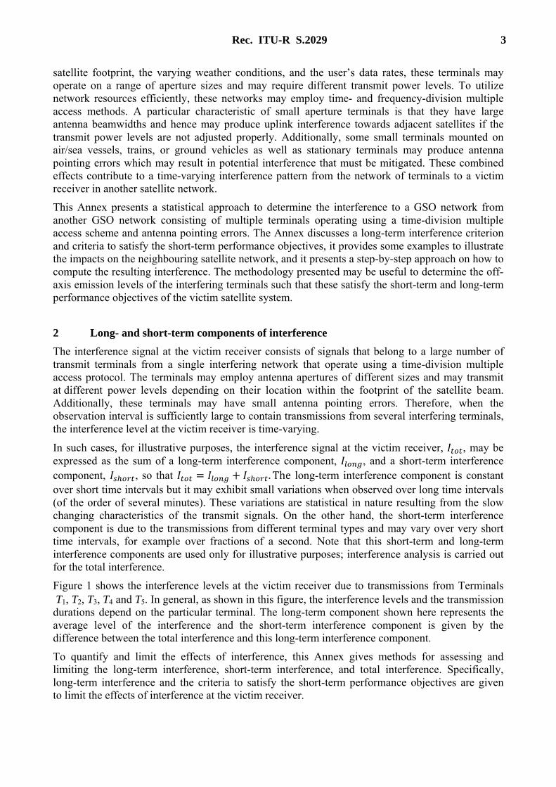
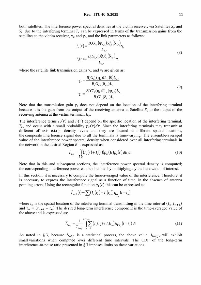
The interfering and the victim satellite networks are shown in Fig. 2. The transmit terminals of the interfering network are denoted by , , … , , as shown here. This figure shows the victim and interfering satellites, and ; wanted terminal, ; and victim receiver, . The analysis aims at quantifying the interference generated by the network of terminals , , … , , to the victim satellite network. The interfering terminals are operating in a time-division multiple access manner with only a single terminal transmitting at a particular time instant in a narrow frequency band of interest. Note that the terminals may operate in a wide frequency band and in a frequency multiple access manner; the interference in this wide frequency band is computed by summing the interference in each narrow frequency band. In Fig. 2, it is assumed that satellites and employ the same frequency translation from the uplink to the downlink.

10 Rec. ITU-R S.2029

FIGURE 2

Interference paths from Terminals T1, T2, … , Tr , to the victim receiver Rv, via Satellites Si and Sv. Ci and Cv denote the beam centres of Si and Sv on the ground; O is the origin from which the distances

to the terminal locations are measured

S.2029-02

Si – Interferingsatellite

Sv – Victimsatellite

Tr – Interferingtransmitter

Rv – Victimreceiver Tv – Wanted

transmitter

Wantedsignalδi ,r

ηi

ψr,v

Ci

Cvr

r1

r2

T1

O

ψv,i

δv, r

T2

ηv

Assuming the interfering terminals are transmitting in a random manner, the time instant at which a particular interfering terminal is transmitting can be represented by a location dependent random variable. The probability density function (PDF) of this random variable is denoted by . When all the interfering terminals are in a Region R, it follows that ( ) = 1.

The interfering terminals may consist of terminals with different antenna aperture sizes. The off-axis e.i.r.p. density pattern of a general terminal located at r is denoted by E. The PDF of the e.i.r.p. density patterns, when considered over all interfering terminals, is denoted by p . Since this is a PDF, it follows that ( ) = 1, where the integral is over all possible values of E.

The antenna pointing error at a terminal located r, which is the angle between the desired and actual directions of the antenna boresight, is denoted by ϕ . These antenna pointing errors may vary slowly and are statistically independent for different terminals. In this Annex it is assumed that elevation and azimuth components of this antenna pointing error, denoted by ϕ , and ϕ , , are available. Also, the PDFs of these antenna pointing error components, and , are assumed to be known.

In the long-term interference criterion it is necessary to compute the time-averaged value of the interference. To facilitate this it is useful to represent the time-dependent transmission pattern of the interfering terminals as shown in Fig. 1. Suppose the Terminal , located at ,transmits in the time interval ( , ). The transmission sequence of these terminals is , , ,…., and the corresponding sequence of transmission intervals are: ( , ), ( , ),( , ), …. In order to represent this denote by ( ) a unit pulse of width τ so that ( ) = 1 in the interval (0, τ), and zero outside this interval. Then the time-dependent transmission pattern of the terminals can be expressed as ∑ ( − ) where τ = ( − ). 7 Determining the long-term interference

The long-term interference is the time-averaged value, in a time interval of , of the interference in the absence of antenna pointing errors. The signal paths from the interfering terminals to the victim receiver via the interfering and victim satellites are shown in Fig. 2. As noted before, in this analysis translation between the uplink and the downlink frequencies is assumed to be the same at

Rec. ITU-R S.2029 11

both satellites. The interference power spectral densities at the victim receiver, via Satellites and , due to the interfering terminal can be expressed in terms of the transmission gains from the

satellites to the victim receiver, γ and γ , and the link parameters as follows:

( ) ( ) ( )

( ) ( ) ( )i

ru

ris

irrtri

vru

rvs

vrvrrtrv

L

GGBrI

L

GGBrI

γδ

=

γδψ

=

,

,,,

,

,,,,

0 (8)

where the satellite link transmission gains γ and γ are given as:

( )

dris

irr

ruivvrisit

si

i

dvvs

vrv

vuvrvsvt

sv

v

LGB

LGGB

LGB

LGGB

)(

)()(

)(

0)(

,,

,,,,

,,

,,,

δψη

=γ

δη

=γ

(9)

Note that the transmission gain γ does not depend on the location of the interfering terminal because it is the gain from the output of the receiving antenna at Satellite to the output of the receiving antenna at the victim terminal, .

The interference terms ( ) and ( ) depend on the specific location of the interfering terminal, , and occur with a small probability ( ) . Since the interfering terminals may transmit at

different off-axis e.i.r.p. density levels and they are located at different spatial locations, the composite interference signal due to all the terminals is time-varying. The ensemble-averaged value of the interference power spectral density when considered over all interfering terminals in the network in the desired Region R is expressed as:

( ) ( )( ) ( ) ( ) drdErpEprIrII rE

ER

ivavg ~

, += (10)

Note that in this and subsequent sections, the interference power spectral density is computed; the corresponding interference power can be obtained by multiplying by the bandwidth of interest.

In this section, it is necessary to compute the time-averaged value of the interference. Therefore, it is necessary to express the interference signal as a function of time, in the absence of antenna pointing errors. Using the rectangular function ( ) this can be expressed as:

( ) ( ) ( )( ) ( )nnn

ninvtot ttqrIrItI −τ+= ~

0,

where is the spatial location of the interfering terminal transmitting in the time interval ( , ) and = ( − ).The desired long-term interference component is the time-averaged value of the above and is expressed as:

( ) ( )( ) ( )dtttqrIrIT

IlongTt

t

nnn

ninvlong

long 1~

+

−τ+= (11)

As noted in § 3, because , is a statistical process, the above value, , will exhibit small variations when computed over different time intervals. The CDF of the long-term interference-to-noise ratio presented in § 3 imposes limits on these variations.


8 Expressing the short-term performance objective criterion

The short-term performance objective criterion in terms of the C/N ratio degradation variables was expressed in § 4.2. In this section, expressions will be given to determine these C/N ratio degradations in terms of the link variables of the satellite network shown in Fig. 2.

8.1 Degradation of the C/N ratio due to rain fading in the presence of long-term interference

The degradation of the C/N ratio due to rain fading in the presence of the long-term interference

component was expressed as = ( / )( / ) in § 4.1. In this subsection, this degradation will be

computed in terms of the specific link variables.

The C/N ratio under clear-sky conditions can be expressed as:

( )longi

csINNN

CNC ~/

,+++

=↑↑↓

(12)

where the variables , ↓, ↑ and ↑, are given by:

s

iiisvvvv

vu

vvs

vrv kNkNkNL

GBC Θγ=Θγ=Θ=γ

δ= ↑↑↓ ,

,

,, ; ; ;)(

Note that in equation (12), and later in § 8.2, the C/N ratio is expressed in terms of the carrier, noise and interference power spectral densities. The corresponding power can be obtained by multiplying these by the bandwidth of interest.

Next, consider the C/N ratio in the presence of rain fading

( ))/(

~)/11(//

//

,, ↓↑↓↓↑↓↑↓

↓↑

+−+++=

AAIANANANN

AACNC

ilongri

s (13)

Here it is assumed that the orbital separation between the satellites and is very small so that the downlink fade terms from these satellites are the same. Also, it is assumed that the uplink fade terms from the interfering terminals are approximately the same and given by ↑, . This is reasonable for a coverage area of a few hundred kilometres. If this is not the case, the last term in the denominator should be appropriately modified to account for the location-dependent rain attenuation term, ↑, ( ). The degradation of the C/N ratio in the static case is defined by = ( / )( / ) . Substituting the values

for ( / ) and ( / ) from equations (12) and (13) it can be shown that:

Zs = A↑ × (A↓d1 + d2 + d3 / A↑,i ) (14)

where the variables , and are defined as:

longi

long

longi

ri

longi

r

INNN

Id

INNN

NNNd

INNN

NNd ~

~ ;~ ;~

,

3

,

,2

,

1 +++=

+++−+

=+++

+=

↑↑↓↑↑↓

↑↑

↑↑↓

↓

Note that ( + + ) = 1. In order to express the parameters , and in terms of the satellite link variables, introduce the following variables:

↓↓↓

↑

↓

↑ ====N

Ic

N

Nc

N

Nc

N

Nc longri

~ ; ; ; 43

,21


Substituting these variables in , and above:

421

43

421

3212

421

31 1

;1

;1

1

ccc

cd

ccc

cccd

ccc

cd

+++=

+++−+=

++++=

The variables , and can be expressed in terms of the satellite link parameters as:

v

long

v

ri

v

si

vv

sv

k

Icccc

Θ=

ΘΘ=γ

ΘΘ=γ

ΘΘ=

~ ; ; ; 4321

Since the rain fades are typically available in dB units, the C/N ratio degradation variable in equation (14) can be analysed conveniently when it is expressed in logarithmic units. Expressing and the rain fades in dB units:

Z s = A↑ +10 log 10A↓/10 d1 + d2 +10−A↑,i /10 d3( )

(15)

The CDF of Zs, PZs

z( ) = Pr Zs

≤ z{ }, can be determined analytically when the PDFs of the rain

attenuation factors, A↑, A↑,i and ↓A are known. Alternatively, a Monte-Carlo simulation method may

be used to estimate the CDF of ̅ . 8.2 Degradation of the C/N ratio due to rain fading in the presence of total interference

In this section, the degradation of the C/N ratio due to rain fading in the presence of total

interference, = ( / )( / ) is determined in terms of the satellite link parameters.

The long-term interference component in § 7 was determined when the interfering terminals are transmitting without antenna pointing errors. Antenna pointing errors of the terminals are taken into consideration in this section. The antenna pointing error at is denoted by ϕ . In the presence of antenna pointing errors the interference terms in equation (8) are expressed as:

( ) ( )( ) ( )

( ) ( )( ) ( )i

ru

ris

irrirrtri

vru

rvs

vrrvrrtrv

L

GGBrI

L

GGBrI

γδϕψ

=

γδϕψ

=

,

,,,,

,

,,,,

(16)

where the dependence of the off-axis angles ψ , and ψ , on ϕ is shown explicitly. The total interference in the presence of antenna pointing errors is now = ( ) + ( ) . The antenna pointing errors are usually available in terms of their errors in the azimuth and elevation directions, ϕ , and ϕ , . Annex 1 of Recommendation ITU-R S.1857 gives a method for determining the angles ψ , (ϕ ) and ψ , (ϕ ) using the available azimuth and elevation error angles.

The C/N ratio at the victim receiver due to rain fading in the presence of total interference is expressed as:

( ))/(

~)/11(//

//

,, ↓↑↓↓↑↓↑↓

↓↑

+−+++=

AAIANANANN

AACNC

itotri

t (17)

Similar to the derivation in the preceding section, the degradation in the C/N ratio in this case,( ) ( )( )tcst NCNCZ ///10log= , is expressed as:

+++= ↑↓ −

↑ 3

10/

2110/

~~1010log10 , dIddAZ tot

AAt

i (18)


where longtottot III~

/~~~ = and the variables , and are as given in the preceding section. The CDF

of ̅ , ( ̅) = Pr ̅ ≤ ̅ , can be determined analytically when the PDFs of the rain attenuation factors and the PDFs noted in § 6 are available. Alternatively, a Monte-Carlo simulation method may be used to estimate the CDF of ̅ . 9 Increase in link degradation due to the short-term interference

The criterion for the short-term performance objectives given in § 4.2 is stated in terms of the complementary CDFs of the link C/N ratio degradation variables, ( ))(1 zP

sZ− and ( ))(1 zPtZ− .

Consider a C/N ratio degradation level of ̅ in rain fading and in the presence of the long-term interference. The link degradation, that is when ̅ exceeds ̅ , in terms of a time percentage in this

case is 1 − ̅ × 100%. Next, consider the total interference to this link.

The link degradation, for the same C/N ratio degradation level of ̅ is 1 − ̅ × 100%.

Therefore, the relative increase in the link degradation due to the presence of the short-term interference is:

%100))(1(

))(1())(1(% ×

−−−−

=jZ

jZjZS zP

zPzPR

t

st (19)

For example, suppose a satellite link is designed to operate so that the C/N ratio for the link is less than ( / ) for only % of the time. According to § 4.2 a link margin should be incorporated so that under rain fading conditions and long-term interference the degradations are limited to at most %× (1 − p /100) of the time. The link margin necessary, ̅ , to satisfy this condition can be

computed using the CDF of the degradation variable as 1 − ̅ = × (1 − /100). Then the short-term interference should be limited so that 1 − ̅ ≤ . It can be see from

equation (19) that for these values % ≤ %.

10 Increase in average interference due to antenna pointing errors

Notice that the long-term interference component, , is computed in the absence of antenna pointing errors and the total interference term, as computed in § 8.2, takes into account antenna pointing errors. The short-term variations of the interference are because of the antenna pointing errors and the time-division multiple access operation of the terminals. Variations due to the latter can be neglected if the average value of , denoted by ⟨ ⟩ and given in equation (10) as ,is considered. This value can be realized when is very large with respect to the average transmission duration of each terminal. The following measure can be used to determine the effect of antenna pointing errors on the average interference:

RL% =Itot − Ilong

Ilong

×100%

(20)

where ⟨ ⟩ is the average value of the total interference. Observe that, in the absence of antenna pointing errors ⟨ ⟩ ≈ ⟨ ⟩, so is negligible.


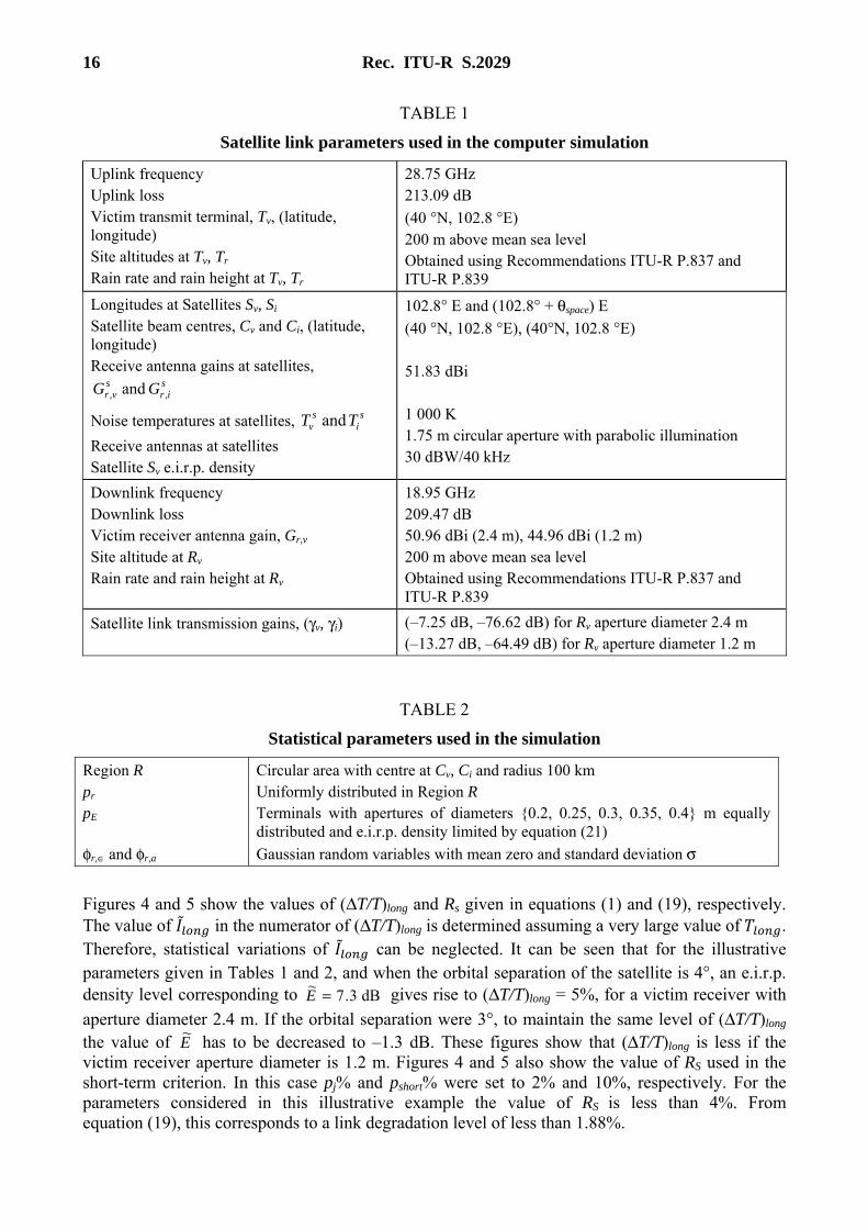
11 Simulation examples

This section provides illustrative computer simulation results obtained from the methodology presented in this Annex. Figure 3 shows the locations of the victim receiver and the interfering terminals with respect to the beam centres of the receive antennas of Si and Sv. As shown here, in this computer simulation the satellite beam centres are coincident and the victim receiver is positioned at this point. The Region R, where the interfering terminals are distributed, is obtained by distributing the transmit terminals uniformly in a circular area with centre Cv (or Ci) and a radius of 100 km. The aperture diameters of the interfering terminals are selected randomly from the set {0.2, 0.25, 0.3, 0.35, 0.4} m and their e.i.r.p. density pattern is limited by the following:

°≤ψ<°+−°≤ψ<°+ψ−

°≤ψ<°+−°≤ψ≤°+ψ−

=ψ

18048dB~

10

489.2dB~

log2522

2.97dB~

2

72dB~

log2519

)kHzW/40(dB )(EIRP

E

E

E

E

(21)

where ψ is the off-axis angle and E~

is a parameter that can be used to increase or decrease the off-axis emission levels from the terminals. Note that when = 0the off-axis emission level corresponds to that specified in recommends 4 of Recommendation ITU-R S.524-9 for earth stations operating in GSO networks in the FSS transmitting in the 27.5-30 GHz frequency band. The following simulation results are given for (ΔT/T)long, RS and RL as a function of E

~. The satellite

link parameters and the statistical parameters used in the computer simulations are given in Tables 1 and 2, respectively.

FIGURE 3

Footprints of the victim and interfering satellites and the distribution of the interfering terminals for this simulation. Here Cv and Ci are coinciding and Rv is also assumed to coincide with this point

S.2029-03

Si – Interferingsatellite

Sv – Victimsatellite

Rv – Victim receiver

C Cv i

Footprints of victimand interfering satellite

Region R:interfering terminalsuniformly distributed


TABLE 1

Satellite link parameters used in the computer simulation

Uplink frequency Uplink loss Victim transmit terminal, Tv, (latitude, longitude) Site altitudes at Tv, Tr Rain rate and rain height at Tv, Tr

28.75 GHz 213.09 dB

(40 °N, 102.8 °E) 200 m above mean sea level Obtained using Recommendations ITU-R P.837 and ITU-R P.839

Longitudes at Satellites Sv, Si Satellite beam centres, Cv and Ci, (latitude, longitude) Receive antenna gains at satellites,

sir

svr GG ,, and

Noise temperatures at satellites, si

sv TT and

Receive antennas at satellites Satellite Sv e.i.r.p. density

102.8° E and (102.8° + θspace) E

(40 °N, 102.8 °E), (40°N, 102.8 °E) 51.83 dBi 1 000 K 1.75 m circular aperture with parabolic illumination 30 dBW/40 kHz

Downlink frequency Downlink loss Victim receiver antenna gain, Gr,v Site altitude at Rv Rain rate and rain height at Rv

18.95 GHz 209.47 dB 50.96 dBi (2.4 m), 44.96 dBi (1.2 m) 200 m above mean sea level Obtained using Recommendations ITU-R P.837 and ITU-R P.839

Satellite link transmission gains, (γv, γi) (–7.25 dB, –76.62 dB) for Rv aperture diameter 2.4 m (–13.27 dB, –64.49 dB) for Rv aperture diameter 1.2 m

TABLE 2

Statistical parameters used in the simulation

Region R pr pE

φr,∈ and φr,a

Circular area with centre at Cv, Ci and radius 100 km Uniformly distributed in Region R Terminals with apertures of diameters {0.2, 0.25, 0.3, 0.35, 0.4} m equally distributed and e.i.r.p. density limited by equation (21)

Gaussian random variables with mean zero and standard deviation σ

Figures 4 and 5 show the values of (ΔT/T)long and Rs given in equations (1) and (19), respectively. The value of in the numerator of (ΔT/T)long is determined assuming a very large value of . Therefore, statistical variations of can be neglected. It can be seen that for the illustrative parameters given in Tables 1 and 2, and when the orbital separation of the satellite is 4°, an e.i.r.p. density level corresponding to dB3.7

~ =E gives rise to (ΔT/T)long = 5%, for a victim receiver with

aperture diameter 2.4 m. If the orbital separation were 3°, to maintain the same level of (ΔT/T)long the value of E

~ has to be decreased to –1.3 dB. These figures show that (ΔT/T)long is less if the

victim receiver aperture diameter is 1.2 m. Figures 4 and 5 also show the value of RS used in the short-term criterion. In this case pj% and pshort% were set to 2% and 10%, respectively. For the parameters considered in this illustrative example the value of RS is less than 4%. From equation (19), this corresponds to a link degradation level of less than 1.88%.


FIGURE 4

Variations of (ΔT/T)long and Rs with E~

in (21) for θspace = 4° and σ = 0.5°

S.2029-04

0 1 2 3 4 5 6 7 8

E (dB)˜

0

1

2

3

4

5

6

Inte

rfer

ence

no

ise

tem

p r

atio

(%

), (

T/T

)Δ

lon

g

R = 2.4 mvR = 1.2 mv

0 1 2 3 4 5 6 7 8

E (dB)˜

0

1

2

3

4

5

Sh

ort-

term

no

ise

inc

reas

e ra

tio

(%),

Rs

R = 2.4 mvR = 1.2 mv

FIGURE 5

Variations of (ΔT/T)long and Rs with E~

in (21) for θspace = 3° and σ = 0.5°

S.2029-05

–6 –5 –4 –3 –2 –1 0

E (dB)˜

0

1

2

3

4

5

6

Inte

rfer

ence

noi

se te

mp

rati

o (%

), (

T/T

)Δ

lon

g

R = 2.4 mvR = 1.2 mv

E (dB)˜

0

1

2

3

4

5Sh

ort-

term

no

ise

inc

reas

e ra

tio

(%),

Rs

R = 2.4 mvR = 1.2 mv

–6 –5 –4 –3 –2 –1 0

The value of RL used in equation (20) is shown in Fig. 6 for different values of σ. As noted before, for sufficiently large values of Tlong, the variations of RL are negligible in the absence of antenna pointing errors. This figure shows the gradual increase of RL with increasing values of σ.

FIGURE 6

Variation of RL with standard deviation of antenna pointing errors for orbital separations of 3° and 4°

S.2029-06

0 0.1 0.2 0.3 0.4 0.5 0.6

σ (degrees)

0

5

10

15

θspace = 4°θspace = 3°

R (%

) L

20

12 Conclusions

A new statistical approach to assess the interference of a time variant system consisting of a network of earth stations operating on a time division multiple access scheme was presented in


this Annex. The results served to illustrate the potential degradation on a victim satellite network and showed that the transmit levels of the interfering network terminals can be adjusted to meet the allowable interference and the performance objectives of the victim satellite system. The Appendix

to this Annex provides an illustrative step-by-step process to estimate the CDF of Δ

and RS.

Appendix

An illustrative step-by-step process to estimate the CDF of

and RS

This Appendix provides an illustrative step-by-step process to estimate the CDF of Δ

expressed in § 3 and the relative increase in degradation due to short-term interference, , as expressed in equation (19) of the Annex. These values are estimated for a given off-axis e.i.r.p. density level. The approach presented here is based on Monte-Carlo simulations.

1 Input to the estimation process

Input 1. Satellite link parameters

Uplink and downlink wavelengths λ , λ ; longitudes of , ; latitude and longitude pair at , ; receive antenna gain patterns , , , ;noise temperatures Θ ,Θ ;transmission gains γ , γ .

Noise temperature Θ .

Input 2. Interfering terminals

PDF of spatial distribution of terminals ; PDF of e.i.r.p. density distribution p . Note that the e.i.r.p. density depends on the aperture size of the terminal and the off-axis e.i.r.p. density limit considered.

Antenna pointing errors: PDFs of azimuth and elevation components of antenna pointing error, p , p .Alternatively, these components may be available as vectors of length (defined in Input 5), ϕ , , ϕ , .

Transmission pattern of the terminals: PDF of the transmission duration of the terminals, p , where τ is the transmission duration of a terminal as discussed in § 6.

Input 3. Rain parameters

Rain rate, altitude above mean seal level and rain height for locations of , ,and the representative center of Region R defined by . These parameters can be computed using Recommendations ITU-R P.837 and ITU-R P.839.

Sky noise temperature due to rain Θ .

Input 4. Parameters to compute long- and short-term interference levels


Observation interval for long-term interference, ;time percentage for link degradations in short-term performance objectives, %; and maximum time percentage for short-term interference, p %.

Input 5. Monte-Carlo simulation parameter: sample size of the random vector

2 Estimation of CDF of

Step 1. Generate the transmission times for the interfering terminals

Generate transmission times, τ , according to the PDF, , such that the sum of all

transmission times satisfies ∑ τ < ≤ ∑ τ .

Step 2. Generate the interfering transmit terminals

a) Generate the -dimensional location vector according to the PDF p .

b) Select the e.i.r.p. density of the terminal at each location point according to the PDF .

Step 3. Compute the interference terms ( ) and ( ) a) Angle ψ , . This is computed using the latitudes and longitudes at , and .

b) Angles δ , and δ , . These are computed using the latitudes and longitudes at , , , and .

c) Compute the uplink path loss , .

d) Interference signal ( ) + ( ) using equation (8). Note that , ψ , is the e.i.r.p. density in the direction of and , (0) is the e.i.r.p. density in the direction of .

The -dimensional vector obtained by computing ( ) + ( ) at all location points gives the instantaneous values of the interference in the absence of antenna pointing errors.

Step 4. Compute the long-term interference

a) Construct the interference signal, , ( ), as a function of time as described in § 7.

, ( ) = ∑ ( ) + ( ) q ( − ), where is the component of , = 0 and = ∑ τ .

b) Compute = , ( ) .

Step 5. Estimate CDF of Δ

a) Construct a -dimensional vector by repeating, times, Steps 1 to 4 above.

b) Construct the -dimensional vector ∆ using (1) and the vector.

c) Estimate the CDF of the vector ∆ .

3 Estimation of

Step 1. Generate the interfering transmit terminals

a) Generate the -dimensional location vector according to the PDF .

b) Select the e.i.r.p. density of the terminal at each location point according to the PDF .


Step 2. Compute the -dimensional interference vector ( ) + ( )

Follow Step 3 in § 2 above.

Step 3. CDF of sZ

a) Determine variables , and given in § 8.1 using the satellite link parameters and the -dimensional vector estimated in Step 5 of § 2 above.

b) Determine the variables , and using , and as shown in § 8.1. Note that ,

and are -dimensional vectors.

c) Generate the -dimensional rain attenuation vectors { }{ } { }↓↑↑ AAAi

and ,, using

Recommendation ITU-R P.618-8. Here { }i

A,↑ corresponds to a single representative

location in the Region R as defined by the PDF p .

d) For each realization of ),,(, ↓↑↑ AAAi and ( , , ), compute sZ expressed in

equation (15). This gives a -dimensional vector for sZ .

e) Estimate the CDF of ),( , zPZsZs using this vector.

Step 4. CDF of tZ

a) Generate the -dimensional antenna pointing error vector ϕ

Generate the -dimensional vectors ϕ , and ϕ , using their respective PDFs, p , p . For each realization ϕ , , ϕ , , compute ϕ using the procedure described in Annex 1 of Recommendation ITU-R S.1857.

b) Generate the -dimensional interference vector ( ) + ( ) given in equation (16)

For each realization and ϕ compute ( ) and ( ) as given in equation (16). Construct the -dimensional interference vector from this.

c) Compute the -dimensional vector tZ using this as given in equation (18).

d) Estimate the CDF of ),(, zPZtZt using this vector.

Step 5. Estimate .

a) Compute the link margin necessary under rain fading conditions and long-term interference, ̅ , such that the maximum time allowed for degradations is %× (1 − /100)

( ) ( ).100/1)(1 shortjjZ ppzPs

−×=−

b) Compute the link degradation time with total interference for this link margin, 1− PZt(zj )( ) .

c) Compute RS using equation (19).

Documents

RECOMMENDATION ITU-R S.2029 - Statistical methodology to assess