Recommender Systems Handbook || Data Mining Methods for Recommender Systems

Chapter 2Data Mining Methods for RecommenderSystems

Xavier Amatriain, Alejandro Jaimes, Nuria Oliver, and Josep M. Pujol

Abstract In this chapter, we give an overview of the main Data Mining techniquesused in the context of Recommender Systems. We first describe common prepro-cessing methods such as sampling or dimensionality reduction. Next, we review themost important classification techniques, including Bayesian Networks and SupportVector Machines. We describe the k-means clustering algorithm and discuss severalalternatives. We also present association rules and related algorithms for an effi-cient training process. In addition to introducing these techniques, we survey theiruses in Recommender Systems and present cases where they have been successfullyapplied.

2.1 Introduction

Recommender Systems (RS) typically apply techniques and methodologies fromother neighboring areas – such as Human Computer Interaction (HCI) or Informa-tion Retrieval (IR). However, most of these systems bear in their core an algorithmthat can be understood as a particular instance of a Data Mining (DM) technique.

The process of data mining typically consists of 3 steps, carried out in succes-sion: Data Preprocessing [59], Data Analysis, and Result Interpretation (see Figure2.1). We will analyze some of the most important methods for data preprocessingin Section 2.2. In particular, we will focus on sampling, dimensionality reduction,and the use of distance functions because of their significance and their role in RS.In Sections 2.3 through 2.5, we provide an overview introduction to the data miningmethods that are most commonly used in RS: classification, clustering and associa-

Xavier AmatriainTelefonica Research, Via Augusta, 122, Barcelona 08021, Spain e-mail: [email protected]

Alejandro JaimesYahoo! Research, Av.Diagonal, 177, Barcelona 08018, Spain. Work on the chapter was performedwhile the author was at Telefonica Research. e-mail: [email protected]

Nuria OliverTelefonica Research, Via Augusta, 122, Barcelona 08021, Spain e-mail: [email protected]

Josep M. PujolTelefonica Research, Via Augusta, 122, Barcelona 08021, Spain e-mail: [email protected]

F. Ricci et al. (eds.), Recommender Systems Handbook, DOI 10.1007/978-0-387-85820-3_2, © Springer Science+Business Media, LLC 2011

39

40 Xavier Amatriain, Alejandro Jaimes, Nuria Oliver, and Josep M. Pujol

tion rule discovery (see Figure 2.1 for a detailed view of the different topics coveredin the chapter).

Fig. 2.1: Main steps and methods in a Data Mining problem, with their correspon-dence to chapter sections.

This chapter does not intend to give a thorough review of Data Mining methods,but rather to highlight the impact that DM algorithms have in the RS field, and toprovide an overview of the key DM techniques that have been successfully used.We shall direct the interested reader to Data Mining textbooks (see [28, 73], forexample) or the more focused references that are provided throughout the chapter.

2.2 Data Preprocessing

We define data as a collection of objects and their attributes, where an attribute isdefined as a property or characteristic of an object. Other names for object includerecord, item, point, sample, observation, or instance. An attribute might be also bereferred to as a variable, field, characteristic, or feature.

2 Data Mining Methods for Recommender Systems 41

Real-life data typically needs to be preprocessed (e.g. cleansed, filtered, trans-formed) in order to be used by the machine learning techniques in the analysis step.In this section, we focus on three issues that are of particular importance when de-signing a RS. First, we review different similarity or distance measures. Next, wediscuss the issue of sampling as a way to reduce the number of items in very largecollections while preserving its main characteristics. Finally, we describe the mostcommon techniques to reduce dimensionality.

2.2.1 Similarity Measures

One of the preferred approaches to collaborative filtering (CF) recommenders is touse the kNN classifier that will be described in Section 2.3.1. This classificationmethod – as most classifiers and clustering techniques – is highly dependent ondefining an appropriate similarity or distance measure.

The simplest and most common example of a distance measure is the Euclideandistance:

d(x,y) =

√n

∑k=1

(xk− yk)2 (2.1)

where n is the number of dimensions (attributes) and xk and yk are the kth attributes(components) of data objects x and y, respectively.

The Minkowski Distance is a generalization of Euclidean Distance:

d(x,y) = (n

∑k=1|xk− yk|r)

1r (2.2)

where r is the degree of the distance. Depending on the value of r, the genericMinkowski distance is known with specific names: For r = 1, the city block, (Man-hattan, taxicab or L1 norm) distance; For r = 2, the Euclidean distance; For r→ ∞,the supremum (Lmax norm or L∞ norm) distance, which corresponds to computingthe maximum difference between any dimension of the data objects.

The Mahalanobis distance is defined as:

d(x,y) =√(x− y)σ−1(x− y)T (2.3)

where σ is the covariance matrix of the data.Another very common approach is to consider items as document vectors of an

n-dimensional space and compute their similarity as the cosine of the angle that theyform:

cos(x,y) =(x• y)||x||||y||

(2.4)


where • indicates vector dot product and ||x|| is the norm of vector x. This similarityis known as the cosine similarity or the L2 Norm .

The similarity between items can also be given by their correlation which mea-sures the linear relationship between objects. While there are several correlation co-efficients that may be applied, the Pearson correlation is the most commonly used.Given the covariance of data points x and y Σ , and their standard deviation σ , wecompute the Pearson correlation using:

Pearson(x,y) =Σ(x,y)σx×σy

(2.5)

RS have traditionally used either the cosine similarity (Eq. 2.4) or the Pearsoncorrelation (Eq. 2.5) – or one of their many variations through, for instance, weight-ing schemes – both Chapters 5 and 4 detail the use of different distance functionsfor CF However, most of the other distance measures previously reviewed are pos-sible. Spertus et al. [69] did a large-scale study to evaluate six different similaritymeasures in the context of the Orkut social network. Although their results might bebiased by the particular setting of their experiment, it is interesting to note that thebest response to recommendations were to those generated using the cosine similar-ity. Lathia et al. [48] also carried out a study of several similarity measures wherethey concluded that, in the general case, the prediction accuracy of a RS was not af-fected by the choice of the similarity measure. As a matter of fact and in the contextof their work, using a random similarity measure sometimes yielded better resultsthan using any of the well-known approaches.

Finally, several similarity measures have been proposed in the case of items thatonly have binary attributes. First, the M01, M10, M11, and M00 quantities are com-puted, where M01 = the number of attributes where x was 0 and y was 1, M10 =the number of attributes where x was 1 and y was 0, and so on. From those quan-tities we can compute: The Simple Matching coefficient SMC = numbero f matches

numbero f attributes =M11+M00

M01+M10+M00+M11 ; the Jaccard coefficient JC = M11M01+M10+M11 . The Extended Jac-

card (Tanimoto) coefficient, a variation of JC for continuous or count attributes thatis computed by d = x•y

∥x∥2+∥x∥2−x•y .

2.2.2 Sampling

Sampling is the main technique used in DM for selecting a subset of relevant datafrom a large data set. It is used both in the preprocessing and final data interpretationsteps. Sampling may be used because processing the entire data set is computation-ally too expensive. It can also be used to create training and testing datasets. In thiscase, the training dataset is used to learn the parameters or configure the algorithmsused in the analysis step, while the testing dataset is used to evaluate the model orconfiguration obtained in the training phase, making sure that it performs well (i.e.generalizes) with previously unseen data.


The key issue to sampling is finding a subset of the original data set that is repre-sentative – i.e. it has approximately the same property of interest – of the entire set.The simplest sampling technique is random sampling, where there is an equal prob-ability of selecting any item. However, more sophisticated approaches are possible.For instance, in stratified sampling the data is split into several partitions based ona particular feature, followed by random sampling on each partition independently.

The most common approach to sampling consists of using sampling without re-placement: When an item is selected, it is removed from the population. However, itis also possible to perform sampling with replacement, where items are not removedfrom the population once they have been selected, allowing for the same sample tobe selected more than once.

It is common practice to use standard random sampling without replacement withan 80/20 proportion when separating the training and testing data sets. This meansthat we use random sampling without replacement to select 20% of the instancesfor the testing set and leave the remaining 80% for training. The 80/20 proportionshould be taken as a rule of thumb as, in general, any value over 2/3 for the trainingset is appropriate.

Sampling can lead to an over-specialization to the particular division of the train-ing and testing data sets. For this reason, the training process may be repeated sev-eral times. The training and test sets are created from the original data set, the modelis trained using the training data and tested with the examples in the test set. Next,different training/test data sets are selected to start the training/testing process againthat is repeated K times. Finally, the average performance of the K learned mod-els is reported. This process is known as cross-validation. There are several cross-validation techniques. In repeated random sampling, a standard random samplingprocess is carried out K times. In n-Fold cross validation, the data set is divided inton folds. One of the folds is used for testing the model and the remaining n−1 foldsare used for training. The cross validation process is then repeated n times with eachof the n subsamples used exactly once as validation data. Finally, the leave-one-out(LOO) approach can be seen as an extreme case of n-Fold cross validation wheren is set to the number of items in the data set. Therefore, the algorithms are runas many times as data points using only one of them as a test each time. It shouldbe noted, though, that as Isaksson et al. discuss in [44], cross-validation may beunreliable unless the data set is sufficiently large.

A common approach in RS is to sample the available feedback from the users –e.g. in the form of ratings – to separate it into training and testing. Cross-validationis also common. Although a standard random sampling is acceptable in the generalcase, in others we might need to bias our sampling for the test set in different ways.We might, for instance, decide to sample only from most recent ratings – sincethose are the ones we would be predicting in a real-world situation. We might alsobe interested in ensuring that the proportion of ratings per user is preserved in thetest set and therefore impose that the random sampling is done on a per user basis.However, all these issues relate to the problem of evaluating RS, which is still amatter of research and discussion.


2.2.3 Reducing Dimensionality

It is common in RS to have not only a data set with features that define a high-dimensional space, but also very sparse information in that space – i.e. there arevalues for a limited number of features per object. The notions of density and dis-tance between points, which are critical for clustering and outlier detection, becomeless meaningful in highly dimensional spaces. This is known as the Curse of Di-mensionality. Dimensionality reduction techniques help overcome this problem bytransforming the original high-dimensional space into a lower-dimensionality.

Sparsity and the curse of dimensionality are recurring problems in RS. Even inthe simplest setting, we are likely to have a sparse matrix with thousands of rowsand columns (i.e. users and items), most of which are zeros. Therefore, dimension-ality reduction comes in naturally. Applying dimensionality reduction makes sucha difference and its results are so directly applicable to the computation of the pre-dicted value, that this is now considered to be an approach to RS design, rather thana preprocessing technique.

In the following, we summarize the two most relevant dimensionality reductionalgorithms in the context of RS: Principal Component Analysis (PCA) and Singu-lar Value Decomposition (SVD). These techniques can be used in isolation or as apreprocessing step for any of the other techniques reviewed in this chapter.

2.2.3.1 Principal Component Analysis

Principal Component Analysis (PCA) [45] is a classical statistical method to findpatterns in high dimensionality data sets. PCA allows to obtain an ordered list ofcomponents that account for the largest amount of the variance from the data interms of least square errors: The amount of variance captured by the first componentis larger than the amount of variance on the second component and so on. We canreduce the dimensionality of the data by neglecting those components with a smallcontribution to the variance.

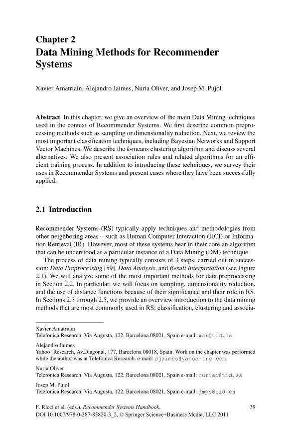
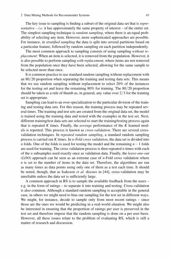
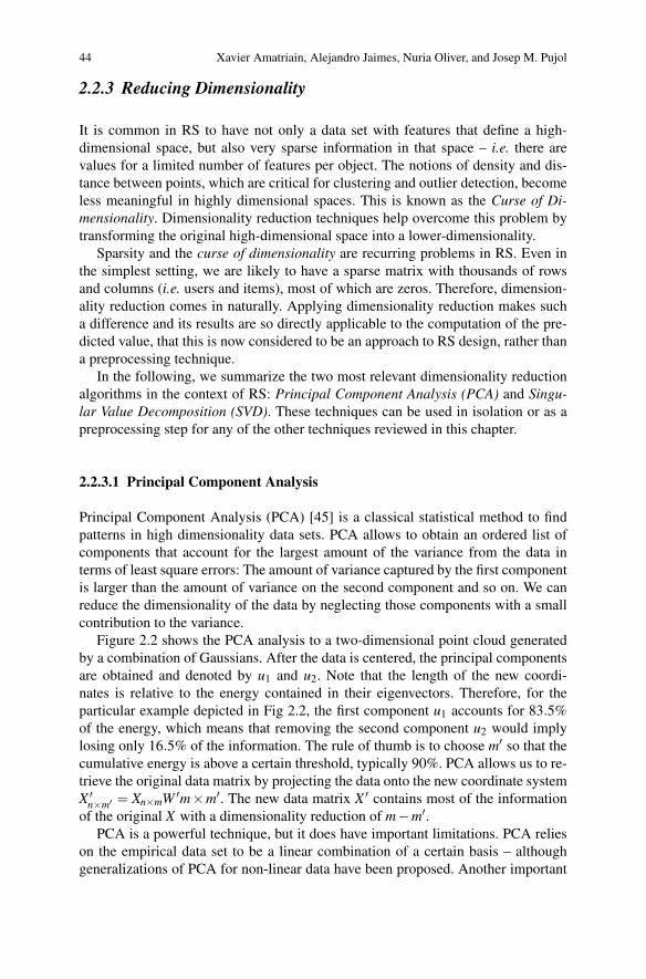
Figure 2.2 shows the PCA analysis to a two-dimensional point cloud generatedby a combination of Gaussians. After the data is centered, the principal componentsare obtained and denoted by u1 and u2. Note that the length of the new coordi-nates is relative to the energy contained in their eigenvectors. Therefore, for theparticular example depicted in Fig 2.2, the first component u1 accounts for 83.5%of the energy, which means that removing the second component u2 would implylosing only 16.5% of the information. The rule of thumb is to choose m′ so that thecumulative energy is above a certain threshold, typically 90%. PCA allows us to re-trieve the original data matrix by projecting the data onto the new coordinate systemX ′n×m′ = Xn×mW ′m×m′. The new data matrix X ′ contains most of the informationof the original X with a dimensionality reduction of m−m′.

PCA is a powerful technique, but it does have important limitations. PCA relieson the empirical data set to be a linear combination of a certain basis – althoughgeneralizations of PCA for non-linear data have been proposed. Another important


−4 −2 2 4

−2

−1

1

2

3

4

u2

u1

Fig. 2.2: PCA analysis of a two-dimensional point cloud from a combination ofGaussians. The principal components derived using PCS are u1 and u2, whose lengthis relative to the energy contained in the components.

assumption of PCA is that the original data set has been drawn from a Gaussiandistribution. When this assumption does not hold true, there is no warranty that theprincipal components are meaningful.

Although current trends seem to indicate that other matrix factorizations tech-niques such as SVD or Non-Negative Matrix Factorization are preferred, earlierworks used PCA. Goldberg et al. proposed an approach to use PCA in the contextof an online joke recommendation system [37]. Their system, known as Eigentaste 1,starts from a standard matrix of user ratings to items. They then select their gauge setby choosing the subset of items for which all users had a rating. This new matrix isthen used to compute the global correlation matrix where a standard 2-dimensionalPCA is applied.

2.2.3.2 Singular Value Decomposition

Singular Value Decomposition [38] is a powerful technique for dimensionality re-duction. It is a particular realization of the Matrix Factorization approach and it istherefore also related to PCA. The key issue in an SVD decomposition is to find alower dimensional feature space where the new features represent “concepts” andthe strength of each concept in the context of the collection is computable. Be-cause SVD allows to automatically derive semantic “concepts” in a low dimensional

1 http://eigentaste.berkeley.edu


space, it can be used as the basis of latent-semantic analysis[24], a very populartechnique for text classification in Information Retrieval .

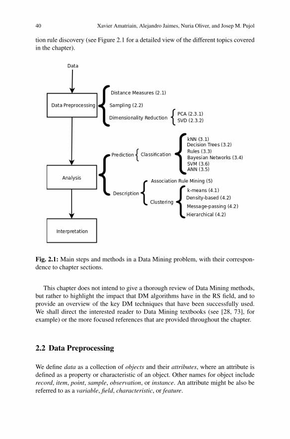
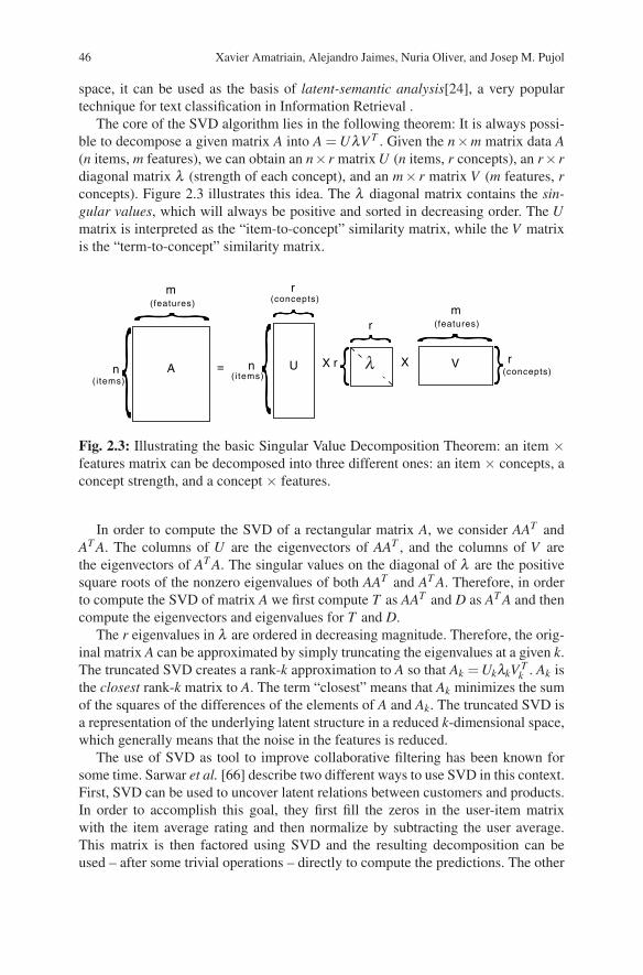
The core of the SVD algorithm lies in the following theorem: It is always possi-ble to decompose a given matrix A into A =UλV T . Given the n×m matrix data A(n items, m features), we can obtain an n× r matrix U (n items, r concepts), an r× rdiagonal matrix λ (strength of each concept), and an m× r matrix V (m features, rconcepts). Figure 2.3 illustrates this idea. The λ diagonal matrix contains the sin-gular values, which will always be positive and sorted in decreasing order. The Umatrix is interpreted as the “item-to-concept” similarity matrix, while the V matrixis the “term-to-concept” similarity matrix.

An

m

= U

r

(items)

(features) (concepts)

X

r

r X V

m

n(items)

(features)

r(concepts)

λ

Fig. 2.3: Illustrating the basic Singular Value Decomposition Theorem: an item ×features matrix can be decomposed into three different ones: an item × concepts, aconcept strength, and a concept × features.

In order to compute the SVD of a rectangular matrix A, we consider AAT andAT A. The columns of U are the eigenvectors of AAT , and the columns of V arethe eigenvectors of AT A. The singular values on the diagonal of λ are the positivesquare roots of the nonzero eigenvalues of both AAT and AT A. Therefore, in orderto compute the SVD of matrix A we first compute T as AAT and D as AT A and thencompute the eigenvectors and eigenvalues for T and D.

The r eigenvalues in λ are ordered in decreasing magnitude. Therefore, the orig-inal matrix A can be approximated by simply truncating the eigenvalues at a given k.The truncated SVD creates a rank-k approximation to A so that Ak =UkλkV T

k . Ak isthe closest rank-k matrix to A. The term “closest” means that Ak minimizes the sumof the squares of the differences of the elements of A and Ak. The truncated SVD isa representation of the underlying latent structure in a reduced k-dimensional space,which generally means that the noise in the features is reduced.

The use of SVD as tool to improve collaborative filtering has been known forsome time. Sarwar et al. [66] describe two different ways to use SVD in this context.First, SVD can be used to uncover latent relations between customers and products.In order to accomplish this goal, they first fill the zeros in the user-item matrixwith the item average rating and then normalize by subtracting the user average.This matrix is then factored using SVD and the resulting decomposition can beused – after some trivial operations – directly to compute the predictions. The other


approach is to use the low-dimensional space resulting from the SVD to improveneighborhood formation for later use in a kNN approach.

As described by Sarwar et al.[65], one of the big advantages of SVD is that thereare incremental algorithms to compute an approximated decomposition. This allowsto accept new users or ratings without having to recompute the model that had beenbuilt from previously existing data. The same idea was later extended and formal-ized by Brand [14] into an online SVD model. The use of incremental SVD methodshas recently become a commonly accepted approach after its success in the NetflixPrize 2. The publication of Simon Funk’s simplified incremental SVD method [35]marked an inflection point in the contest. Since its publication, several improve-ments to SVD have been proposed in this same context (see Paterek’s ensembles ofSVD methods [56] or Kurucz et al. evaluation of SVD parameters [47]).

Finally, it should be noted that different variants of Matrix Factorization (MF)methods such as the Non-negative Matrix Factorization (NNMF) have also beenused[74]. These algorithms are, in essence, similar to SVD. The basic idea is todecompose the ratings matrix into two matrices, one of which contains featuresthat describe the users and the other contains features describing the items. MatrixFactorization methods are better than SVD at handling the missing values by in-troducing a bias term to the model. However, this can also be handled in the SVDpreprocessing step by replacing zeros with the item average. Note that both SVDand MF are prone to overfitting. However, there exist MF variants, such as the Reg-ularized Kernel Matrix Factorization, that can avoid the issue efficiently. The mainissue with MF – and SVD – methods is that it is unpractical to recompute the fac-torization every time the matrix is updated because of computational complexity.However, Rendle and Schmidt-Thieme [62] propose an online method that allowsto update the factorized approximation without recomputing the entire model.

Chapter 5 details the use of SVD and MF in the context of the Netflix Prize andis therefore a good complement to this introduction.

2.2.4 Denoising

Data collected for data-mining purposes might be subject to different kinds of noisesuch as missing values or outliers. Denoising is a very important preprocessing stepthat aims at removing any unwanted effect in the data while maximizing its infor-mation.

In a general sense we define noise as any unwanted artifact introduced in the datacollection phase that might affect the result of our data analysis and interpretation.In the context of RS, we distinguish between natural and malicious noise [55]. Theformer refers to noise that is unvoluntarely introduced byusers when giving feedbackon their preferences. The latter refers to noise that is deliberately introduced in asystem in order to bias the results.

2 http://www.netflixprize.com


It is clear that malicious noise can affect the output of a RS. But, also, we per-formed a study that concluded that the effects of natural noise on the performanceof RS is far from being negligible [4]. In order to address this issue, we designeda denoising approach that is able to improve accuracy by asking some users to re-rate some items [5]. We concluded that accuracy improvements by investing in thispre-processing step could be larger than the ones obtained by complex algorithmoptimizations.

2.3 Classification

A classifier is a mapping between a feature space and a label space, where the fea-tures represent characteristics of the elements to classify and the labels representthe classes. A restaurant RS, for example, can be implemented by a classifier thatclassifies restaurants into one of two categories (good, bad) based on a number offeatures that describe it.

There are many types of classifiers, but in general we will talk about either su-pervised or unsupervised classification. In supervised classification, a set of labelsor categories is known in advance and we have a set of labeled examples whichconstitute a training set. In unsupervised classification, the labels or categories areunknown in advance and the task is to suitably (according to some criteria) organizethe elements at hand. In this section we describe several algorithms to learn super-vised classifiers and will be covering unsupervised classification (i.e. clustering) inSec. 2.4.

2.3.1 Nearest Neighbors

Instance-based classifiers work by storing training records and using them to pre-dict the class label of unseen cases. A trivial example is the so-called rote-learner.This classifier memorizes the entire training set and classifies only if the attributesof the new record match one of the training examples exactly. A more elaborate, andfar more popular, instance-based classifier is the Nearest neighbor classifier (kNN)[22]. Given a point to be classified, the kNN classifier finds the k closest points(nearest neighbors) from the training records. It then assigns the class label accord-ing to the class labels of its nearest-neighbors. The underlying idea is that if a recordfalls in a particular neighborhood where a class label is predominant it is becausethe record is likely to belong to that very same class.

Given a query point q for which we want to know its class l, and a trainingset X = {{x1, l1}...{xn}}, where x j is the j-th element and l j is its class label, thek-nearest neighbors will find a subset Y = {{y1, l1}...{yk}} such that Y ∈ X and∑k

1 d(q,yk) is minimal. Y contains the k points in X which are closest to the querypoint q. Then, the class label of q is l = f ({l1...lk}).


−3 −2 −1 0 1 2 3−3

−2

−1

0

1

2

3

items of cluster 1items of cluster 2item to classify

−3 −2 −1 0 1 2 3−3

−2

−1

0

1

2

3

items of cluster 1items of cluster 2item to classify

?

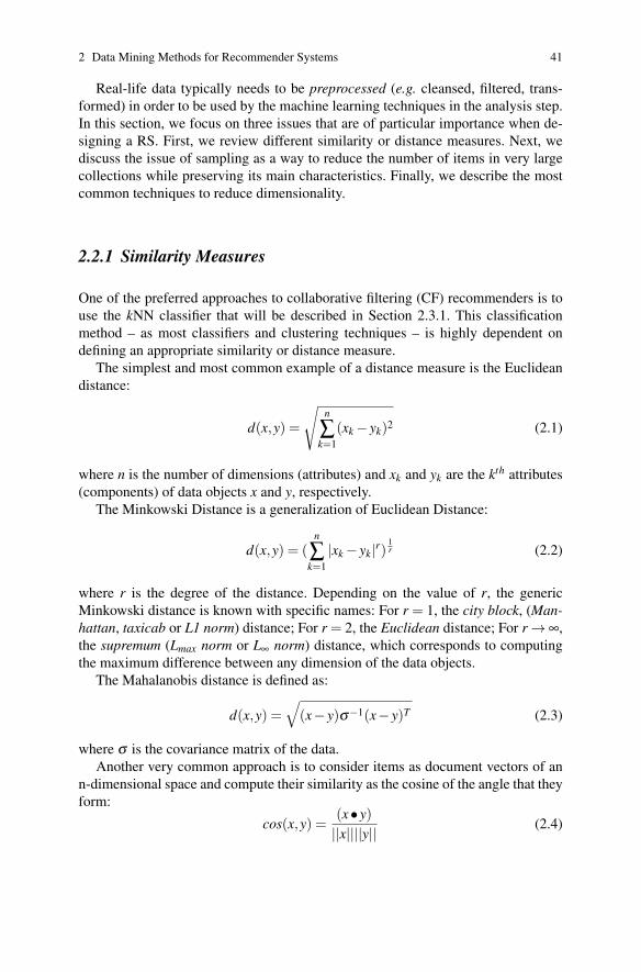
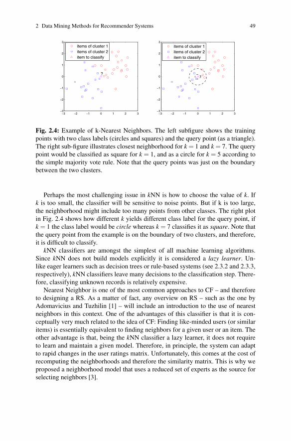
Fig. 2.4: Example of k-Nearest Neighbors. The left subfigure shows the trainingpoints with two class labels (circles and squares) and the query point (as a triangle).The right sub-figure illustrates closest neighborhood for k = 1 and k = 7. The querypoint would be classified as square for k = 1, and as a circle for k = 5 according tothe simple majority vote rule. Note that the query points was just on the boundarybetween the two clusters.

Perhaps the most challenging issue in kNN is how to choose the value of k. Ifk is too small, the classifier will be sensitive to noise points. But if k is too large,the neighborhood might include too many points from other classes. The right plotin Fig. 2.4 shows how different k yields different class label for the query point, ifk = 1 the class label would be circle whereas k = 7 classifies it as square. Note thatthe query point from the example is on the boundary of two clusters, and therefore,it is difficult to classify.

kNN classifiers are amongst the simplest of all machine learning algorithms.Since kNN does not build models explicitly it is considered a lazy learner. Un-like eager learners such as decision trees or rule-based systems (see 2.3.2 and 2.3.3,respectively), kNN classifiers leave many decisions to the classification step. There-fore, classifying unknown records is relatively expensive.

Nearest Neighbor is one of the most common approaches to CF – and thereforeto designing a RS. As a matter of fact, any overview on RS – such as the one byAdomavicius and Tuzhilin [1] – will include an introduction to the use of nearestneighbors in this context. One of the advantages of this classifier is that it is con-ceptually very much related to the idea of CF: Finding like-minded users (or similaritems) is essentially equivalent to finding neighbors for a given user or an item. Theother advantage is that, being the kNN classifier a lazy learner, it does not requireto learn and maintain a given model. Therefore, in principle, the system can adaptto rapid changes in the user ratings matrix. Unfortunately, this comes at the cost ofrecomputing the neighborhoods and therefore the similarity matrix. This is why weproposed a neighborhood model that uses a reduced set of experts as the source forselecting neighbors [3].


The kNN approach, although simple and intuitive, has shown good accuracy re-sults and is very amenable to improvements. As a matter of fact, its supremacy asthe de facto standard for CF recommendation has only been challenged recently byapproaches based on dimensionality reduction such as the ones reviewed in Section2.2.3. That said, the traditional kNN approach to CF has experienced improvementsin several directions. For instance, in the context of the Netflix Prize, Bell and Ko-ren propose a method to remove global effects such as the fact that some items mayattract users that consistently rate lower. They also propose an optimization methodfor computing interpolating weights once the neighborhood is created.

See Chapters 5 and 4 for more details on enhanced CF techniques based on theuse of neighborhoods.

2.3.2 Decision Trees

Decision trees [61, 63] are classifiers on a target attribute (or class) in the form of atree structure. The observations (or items) to classify are composed of attributes andtheir target value. The nodes of the tree can be: a) decision nodes, in these nodes asingle attribute-value is tested to determine to which branch of the subtree applies.Or b) leaf nodes which indicate the value of the target attribute.

There are many algorithms for decision tree induction: Hunts Algorithm, CART,ID3, C4.5, SLIQ, SPRINT to mention the most common. The recursive Hunt al-gorithm, which is one of the earliest and easiest to understand, relies on the testcondition applied to a given attribute that discriminates the observations by theirtarget values. Once the partition induced by the test condition has been found, thealgorithm is recursively repeated until a partition is empty or all the observationshave the same target value.

Splits can be decided by maximizing the information gain, defined as follows,

∆i = I(parent)−ki

∑j=1

N(v j)I(v j)

N(2.6)

where ki are values of the attribute i, N is the number of observations, v j is the j-th partition of the observations according to the values of attribute i. Finally, I is afunction that measures node impurity. There are different measures of impurity: GiniIndex, Entropy and misclassification error are the most common in the literature.

Decision tree induction stops once all observations belong to the same class (orthe same range in the case of continuous attributes). This implies that the impurityof the leaf nodes is zero. For practical reasons, however, most decision trees imple-mentations use pruning by which a node is no further split if its impurity measureor the number of observations in the node are below a certain threshold.

The main advantages of building a classifier using a decision tree is that it isinexpensive to construct and it is extremely fast at classifying unknown instances.Another appreciated aspect of decision tree is that they can be used to produce a set


of rules that are easy to interpret (see section 2.3.3) while maintaining an accuracycomparable to other basic classification techniques.

Decision trees may be used in a model-based approach for a RS. One possibil-ity is to use content features to build a decision tree that models all the variablesinvolved in the user preferences. Bouza et al. [12] use this idea to construct a Deci-sion Tree using semantic information available for the items. The tree is built afterthe user has rated only two items. The features for each of the items are used tobuild a model that explains the user ratings. They use the information gain of everyfeature as the splitting criteria. It should be noted that although this approach is in-teresting from a theoretical perspective, the precision they report on their system isworse than that of recommending the average rating.

As it could be expected, it is very difficult and unpractical to build a decisiontree that tries to explain all the variables involved in the decision making process.Decision trees, however, may also be used in order to model a particular part ofthe system. Cho et al. [18], for instance, present a RS for online purchases thatcombines the use of Association Rules (see Section 2.5) and Decision Trees. TheDecision Tree is used as a filter to select which users should be targeted with recom-mendations. In order to build the model they create a candidate user set by selectingthose users that have chosen products from a given category during a given timeframe. In their case, the dependent variable for building the decision tree is cho-sen as whether the customer is likely to buy new products in that same category.Nikovski and Kulev [54] follow a similar approach combining Decision Trees andAssociation Rules. In their approach, frequent itemsets are detected in the purchasedataset and then they apply standard tree-learning algorithms for simplifying therecommendations rules.

Another option to use Decision Trees in a RS is to use them as a tool for itemranking. The use of Decision Trees for ranking has been studied in several settingsand their use in a RS for this purpose is fairly straightforward [7, 17].

2.3.3 Ruled-based Classifiers

Rule-based classifiers classify data by using a collection of “if . . . then . . .” rules.The rule antecedent or condition is an expression made of attribute conjunctions.The rule consequent is a positive or negative classification.

We say that a rule r covers a given instance x if the attributes of the instancesatisfy the rule condition. We define the coverage of a rule as the fraction of recordsthat satisfy its antecedent. On the other hand, we define its accuracy as the fractionof records that satisfy both the antecedent and the consequent. We say that a clas-sifier contains mutually exclusive rules if the rules are independent of each other –i.e. every record is covered by at most one rule. Finally we say that the classifier hasexhaustive rules if they account for every possible combination of attribute values–i.e. each record is covered by at least one rule.


In order to build a rule-based classifier we can follow a direct method to extractrules directly from data. Examples of such methods are RIPPER, or CN2. On theother hand, it is common to follow an indirect method and extract rules from otherclassification models such as decision trees or neural networks.

The advantages of rule-based classifiers are that they are extremely expressivesince they are symbolic and operate with the attributes of the data without anytransformation. Rule-based classifiers, and by extension decision trees, are easy tointerpret, easy to generate and they can classify new instances efficiently.

In a similar way to Decision Tress, however, it is very difficult to build a completerecommender model based on rules. As a matter of fact, this method is not verypopular in the context of RS because deriving a rule-based system means that weeither have some explicit prior knowledge of the decision making process or thatwe derive the rules from another model such a decision tree. However a rule-basedsystem can be used to improve the performance of a RS by injecting partial domainknowledge or business rules. Anderson et al. [6], for instance, implemented a CFmusic RS that improves its performance by applying a rule-based system to theresults of the CF process. If a user rates an album by a given artist high, for instance,predicted ratings for all other albums by this artist will be increased.

Gutta et al. [29] implemented a rule-based RS for TV content. In order to do,so they first derived a C4.5 Decision Tree that is then decomposed into rules forclassifying the programs. Basu et al. [9] followed an inductive approach using theRipper [20] system to learn rules from data. They report slightly better results whenusing hybrid content and collaborative data to learn rules than when following apure CF approach.

2.3.4 Bayesian Classifiers

A Bayesian classifier [34] is a probabilistic framework for solving classificationproblems. It is based on the definition of conditional probability and the Bayes the-orem. The Bayesian school of statistics uses probability to represent uncertaintyabout the relationships learned from the data. In addition, the concept of priors isvery important as they represent our expectations or prior knowledge about what thetrue relationship might be. In particular, the probability of a model given the data(posterior) is proportional to the product of the likelihood times the prior proba-bility (or prior). The likelihood component includes the effect of the data while theprior specifies the belief in the model before the data was observed.

Bayesian classifiers consider each attribute and class label as (continuous or dis-crete) random variables. Given a record with N attributes (A1,A2, ...,AN), the goalis to predict class Ck by finding the value of Ck that maximizes the posterior prob-ability of the class given the data P(Ck|A1,A2, ...,AN). Applying Bayes’ theorem,P(Ck|A1,A2, ...,AN) ∝ P(A1,A2, ...,AN |Ck)P(Ck)

A particular but very common Bayesian classifier is the Naive Bayes Classifier.In order to estimate the conditional probability, P(A1,A2, ...,AN |Ck), a Naive Bayes


Classifier assumes the probabilistic independence of the attributes – i.e. the pres-ence or absence of a particular attribute is unrelated to the presence or absence of anyother. This assumption leads to P(A1,A2, ...,AN |Ck)=P(A1|Ck)P(A2|Ck)...P(AN |Ck).

The main benefits of Naive Bayes classifiers are that they are robust to isolatednoise points and irrelevant attributes, and they handle missing values by ignoringthe instance during probability estimate calculations. However, the independenceassumption may not hold for some attributes as they might be correlated. In thiscase, the usual approach is to use the so-called Bayesian Belief Networks (BBN)(or Bayesian Networks, for short). BBN’s use an acyclic graph to encode the de-pendence between attributes and a probability table that associates each node to itsimmediate parents. BBN’s provide a way to capture prior knowledge in a domainusing a graphical model. In a similar way to Naive Bayes classifiers, BBN’s handleincomplete data well and they are quite robust to model overfitting.

Bayesian classifiers are particularly popular for model-based RS. They are oftenused to derive a model for content-based RS. However, they have also been usedin a CF setting. Ghani and Fano [36], for instance, use a Naive Bayes classifier toimplement a content-based RS. The use of this model allows for recommendingproducts from unrelated categories in the context of a department store.

Miyahara and Pazzani [52] implement a RS based on a Naive Bayes classifier.In order to do so, they define two classes: like and don’t like. In this context theypropose two ways of using the Naive Bayesian Classifier: The Transformed DataModel assumes that all features are completely independent, and feature selectionis implemented as a preprocessing step. On the other hand, the Sparse Data Modelassumes that only known features are informative for classification. Furthermore, itonly makes use of data which both users rated in common when estimating proba-bilities. Experiments show both models to perform better than a correlation-basedCF.

Pronk et al. [58] use a Bayesian Naive Classifier as the base for incorporatinguser control and improving performance, especially in cold-start situations. In orderto do so they propose to maintain two profiles for each user: one learned from therating history, and the other explicitly created by the user. The blending of bothclassifiers can be controlled in such a way that the user-defined profile is favoredat early stages, when there is not too much rating history, and the learned classifiertakes over at later stages.

In the previous section we mentioned that Gutta et al. [29] implemented arule-based approach in a TV content RS. Another of the approaches they testedwas a Bayesian classifier. They define a two-class classifier, where the classes arewatched/not watched. The user profile is then a collection of attributes together withthe number of times they occur in positive and negative examples. This is used tocompute prior probabilities that a show belongs to a particular class and the con-ditional probability that a given feature will be present if a show is either positiveor negative. It must be noted that features are, in this case, related to both content–i.e. genre – and contexts –i.e. time of the day. The posteriori probabilities for a newshow are then computed from these.


Breese et al. [15] implement a Bayesian Network where each node correspondsto each item. The states correspond to each possible vote value. In the network, eachitem will have a set of parent items that are its best predictors. The conditional prob-ability tables are represented by decision trees. The authors report better results forthis model than for several nearest-neighbors implementations over several datasets.

Hierarchical Bayesian Networks have also been used in several settings as a wayto add domain-knowledge for information filtering [78]. One of the issues with hier-archical Bayesian networks, however, is that it is very expensive to learn and updatethe model when there are many users in it. Zhang and Koren [79] propose a varia-tion over the standard Expectation-Maximization (EM) model in order to speed upthis process in the scenario of a content-based RS.

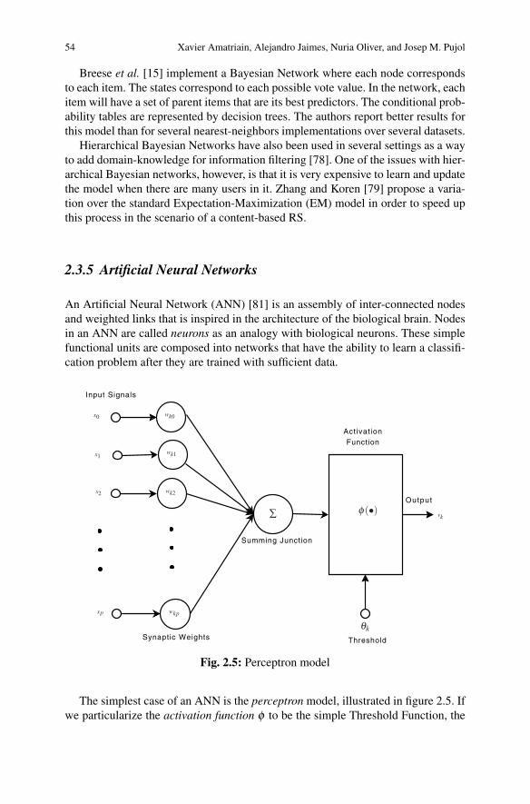
2.3.5 Artificial Neural Networks

An Artificial Neural Network (ANN) [81] is an assembly of inter-connected nodesand weighted links that is inspired in the architecture of the biological brain. Nodesin an ANN are called neurons as an analogy with biological neurons. These simplefunctional units are composed into networks that have the ability to learn a classifi-cation problem after they are trained with sufficient data.

Input Signals

Synaptic Weights

Summing Junction

ActivationFunction

Output

Threshold

wk0

wk1

wk2

wkp

x0

x1

x2

xp

∑ φ(•)

θk

vk

Fig. 2.5: Perceptron model

The simplest case of an ANN is the perceptron model, illustrated in figure 2.5. Ifwe particularize the activation function ϕ to be the simple Threshold Function, the


output is obtained by summing up each of its input value according to the weightsof its links and comparing its output against some threshold θk. The output functioncan be expressed using Eq. 2.7. The perceptron model is a linear classifier that hasa simple and efficient learning algorithm. But, besides the simple Threshold Func-tion used in the Perceptron model, there are several other common choices for theactivation function such as sigmoid, tanh, or step functions.

yk =

{1, if ∑xiwki ≥ θk

0, if ∑xiwki < θk(2.7)

An ANN can have any number of layers. Layers in an ANN are classified intothree types: input, hidden, and output. Units in the input layer respond to data thatis fed into the network. Hidden units receive the weighted output from the inputunits. And the output units respond to the weighted output from the hidden unitsand generate the final output of the network. Using neurons as atomic functionalunits, there are many possible architectures to put them together in a network. But,the most common approach is to use the feed-forward ANN. In this case, signals arestrictly propagated in one way: from input to output.

The main advantages of ANN are that – depending on the activation function– they can perform non-linear classification tasks, and that, due to their parallelnature, they can be efficient and even operate if part of the network fails. The maindisadvantage is that it is hard to come up with the ideal network topology for agiven problem and once the topology is decided this will act as a lower bound forthe classification error. ANN’s belong to the class of sub-symbolic classifiers, whichmeans that they provide no semantics for inferring knowledge – i.e. they promote akind of black-box approach.

ANN’s can be used in a similar way as Bayesian Networks to construct model-based RS’s. However, there is no conclusive study to whether ANN introduce anyperformance gain. As a matter of fact, Pazzani and Billsus [57] did a comprehen-sive experimental study on the use of several machine learning algorithms for website recommendation. Their main goal was to compare the simple naive BayesianClassifier with computationally more expensive alternatives such as Decision Treesand Neural Networks. Their experimental results show that Decision Trees performsignificantly worse. On the other hand ANN and the Bayesian classifier performedsimilarly. They conclude that there does not seem to be a need for nonlinear clas-sifiers such as the ANN. Berka et al. [31] used ANN to build an URL RS for webnavigation. They implemented a content-independent system based exclusively ontrails – i.e. associating pairs of domain names with the number of people who tra-versed them. In order to do so they used feed-forward Multilayer Perceptrons trainedwith the Backpropagation algorithm.

ANN can be used to combine (or hybridize) the input from several recommen-dation modules or data sources. Hsu et al. [30], for instance, build a TV recom-mender by importing data from four different sources: user profiles and stereo-types; viewing communities; program metadata; and viewing context. They use theback-propagation algorithm to train a three-layered neural network. Christakou and


Stafylopatis [19] also built a hybrid content-based CF RS. The content-based rec-ommender is implemented using three neural networks per user, each of them cor-responding to one of the following features: “kinds”, “stars”, and “synopsis”. Theytrained the ANN using the Resilient Backpropagation method.

2.3.6 Support Vector Machines

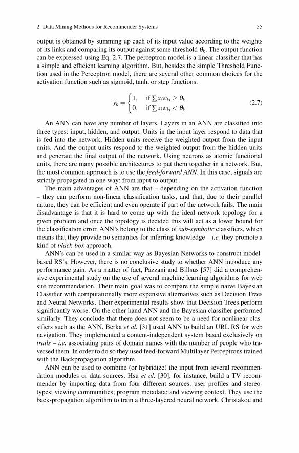
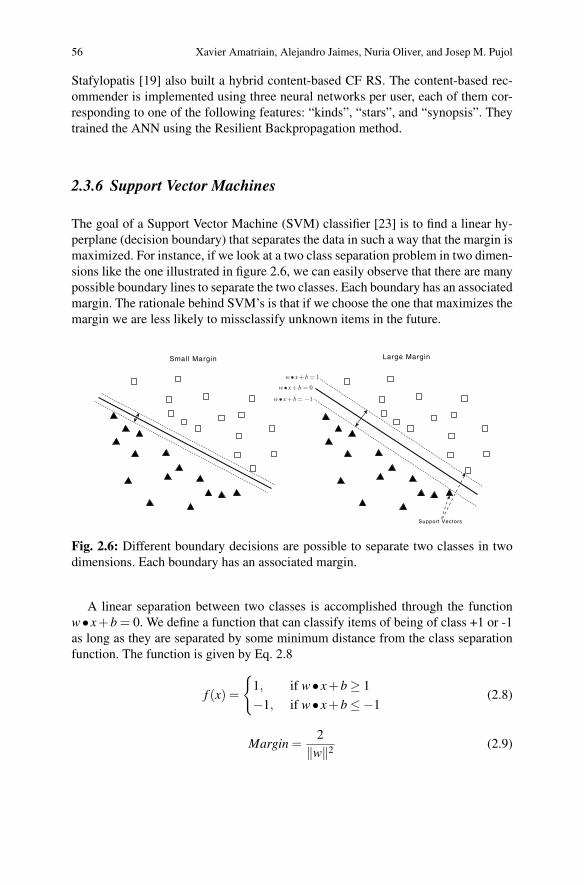
The goal of a Support Vector Machine (SVM) classifier [23] is to find a linear hy-perplane (decision boundary) that separates the data in such a way that the margin ismaximized. For instance, if we look at a two class separation problem in two dimen-sions like the one illustrated in figure 2.6, we can easily observe that there are manypossible boundary lines to separate the two classes. Each boundary has an associatedmargin. The rationale behind SVM’s is that if we choose the one that maximizes themargin we are less likely to missclassify unknown items in the future.

Large MarginSmall Margin

Support Vectors

w • x+b = 0

w • x+b = 1

w • x+b = −1

Fig. 2.6: Different boundary decisions are possible to separate two classes in twodimensions. Each boundary has an associated margin.

A linear separation between two classes is accomplished through the functionw• x+b = 0. We define a function that can classify items of being of class +1 or -1as long as they are separated by some minimum distance from the class separationfunction. The function is given by Eq. 2.8

f (x) =

{1, if w• x+b≥ 1−1, if w• x+b≤−1

(2.8)

Margin =2∥w∥2 (2.9)


Following the main rationale for SVM’s, we would like to maximize the marginbetween the two classes, given by equation 2.9. This is in fact equivalent to mini-mizing the inverse value L(w) = ∥w∥2

2 but subjected to the constraints given by f (x).This is a constrained optimization problem and there are numerical approaches tosolve it (e.g., quadratic programming).

If the items are not linearly separable we can decide to turn the svm into a softmargin classifier by introducing a slack variable. In this case the formula to mini-mize is given by equation 2.10 subject to the new definition of f (x) in equation 2.11.On the other hand, if the decision boundary is not linear we need to transform datainto a higher dimensional space . This is accomplished thanks to a mathematicaltransformation known as the kernel trick. The basic idea is to replace the dot prod-ucts in equation 2.8 by a kernel function. There are many different possible choicesfor the kernel function such as Polynomial or Sigmoid. But the most common kernelfunctions are the family of Radial Basis Function (RBF).

L(w) =∥w∥2

2+C

N

∑i=1

ε (2.10)

f (x) =

{1, if w• x+b≥ 1− ε−1, if w• x+b≤−1+ ε

(2.11)

Support Vector Machines have recently gained popularity for their performanceand efficiency in many settings. SVM’s have also shown promising recent resultsin RS. Kang and Yoo [46], for instance, report on an experimental study that aimsat selecting the best preprocessing technique for predicting missing values for anSVM-based RS. In particular, they use SVD and Support Vector Regression. TheSupport Vector Machine RS is built by first binarizing the 80 levels of available userpreference data. They experiment with several settings and report best results for athreshold of 32 – i.e. a value of 32 and less is classified as prefer and a higher valueas do not prefer. The user id is used as the class label and the positive and negativevalues are expressed as preference values 1 and 2.

Xu and Araki [76] used SVM to build a TV program RS. They used informa-tion from the Electronic Program Guide (EPG) as features. But in order to reducefeatures they removed words with lowest frequencies. Furthermore, and in order toevaluate different approaches, they used both the Boolean and the Term frequency -inverse document frequency (TFIDF) weighting schemes for features. In the former,0 and 1 are used to represent absence or presence of a term on the content. In thelatter, this is turned into the TFIDF numerical value.

Xia et al.[75] present different approaches to using SVM’s for RS in a CF set-ting. They explore the use of Smoothing Support Vector Machines (SSVM). Theyalso introduce a SSVM-based heuristic (SSVMBH) to iteratively estimate missingelements in the user-item matrix. They compute predictions by creating a classifierfor each user. Their experimental results report best results for the SSVMBH ascompared to both SSVM’s and traditional user-based and item-based CF. Finally,


Oku et al. [27] propose the use of Context-Aware Vector Machines (C-SVM) forcontext-aware RS. They compare the use of standard SVM, C-SVM and an exten-sion that uses CF as well as C-SVM. Their results show the effectiveness of thecontext-aware methods for restaurant recommendations.

2.3.7 Ensembles of Classifiers

The basic idea behind the use of ensembles of classifiers is to construct a set ofclassifiers from the training data and predict class labels by aggregating their pre-dictions. Ensembles of classifiers work whenever we can assume that the classifiersare independent. In this case we can ensure that the ensemble will produce resultsthat are in the worst case as bad as the worst classifier in the ensemble. Therefore,combining independent classifiers of a similar classification error will only improveresults.

In order to generate ensembles, several approaches are possible. The two mostcommon techniques are Bagging and Boosting. In Bagging, we perform samplingwith replacement, building the classifier on each bootstrap sample. Each sample hasprobability (1− 1

N )N of being selected – note that if N is large enough, this converges

to 1− 1e ≈ 0.623. In Boosting we use an iterative procedure to adaptively change

distribution of training data by focusing more on previously misclassified records.Initially, all records are assigned equal weights. But, unlike bagging, weights maychange at the end of each boosting round: Records that are wrongly classified willhave their weights increased while records that are classified correctly will havetheir weights decreased. An example of boosting is the AdaBoost algorithm.

The use of ensembles of classifiers is common practice in the RS field. As amatter of fact, any hybridation technique [16] can be considered an ensemble asit combines in one way or another several classifiers. An explicit example of thisis Tiemann and Pauws’ music recommender, in which they use ensemble learningmethods to combine a social and a content-base RS [70].

Experimental results show that ensembles can produce better results than anyclassifier in isolation. Bell et al. [11], for instance, used a combination of 107 differ-ent methods in their progress prize winning solution to the Netflix challenge. Theystate that their findings show that it pays off more to find substantially different ap-proaches rather than focusing on refining a particular technique. In order to blendthe results from the ensembles they use a linear regression approach and to deriveweights for each classifier, they partition the test dataset into 15 different bins andderive unique coefficients for each of the bins. Different uses of ensembles in thecontext of the Netflix prize can be tracked in other approaches such as in Schclar etal.’s [67] or Toescher et al.’s [71].

The boosting approach has also been used in RS. Freund et al., for instance,present an algorithm called RankBoost to combine preferences [32]. They apply thealgorithm to produce movie recommendations in a CF setting.


2.3.8 Evaluating Classifiers

The most commonly accepted evaluation measure for RS is the Mean Average Erroror Root Mean Squared Error of the predicted interest (or rating) and the measuredone. These measures compute accuracy without any assumption on the purpose ofthe RS. However, as McNee et al. point out [51], there is much more than accuracyto deciding whether an item should be recommended. Herlocker et al. [42] providea comprehensive review of algorithmic evaluation approaches to RS. They suggestthat some measures could potentially be more appropriate for some tasks. However,they are not able to validate the measures when evaluating the different approachesempirically on a class of recommendation algorithms and a single set of data.

A step forward is to consider that the purpose of a “real” RS is to produce a top-Nlist of recommendations and evaluate RS depending on how well they can classifyitems as being recommendable. If we look at our recommendation as a classifica-tion problem, we can make use of well-known measures for classifier evaluationsuch as precision and recall. In the following paragraphs, we will review some ofthese measures and their application to RS evaluation. Note however that learn-ing algorithms and classifiers can be evaluated by multiple criteria. This includeshow accurately they perform the classification, their computational complexity dur-ing training , complexity during classification, their sensitivity to noisy data, theirscalability, and so on. But in this section we will focus only on classification perfor-mance.

In order to evaluate a model we usually take into account the following measures:True Positives (T P): number of instances classified as belonging to class A thattruly belong to class A; True Negatives (T N): number of instances classified as notbelonging to class A and that in fact do not belong to class A; False Positives (FP):number of instances classified as class A but that do not belong to class A; FalseNegatives (FN): instances not classified as belonging to class v but that in fact dobelong to class A.

The most commonly used measure for model performance is its Accuracy de-fined as the ratio between the instances that have been correctly classified (as be-longing or not to the given class) and the total number of instances: Accuracy =(T P + T N)/(T P + T N + FP + FN). However, accuracy might be misleading inmany cases. Imagine a 2-class problem in which there are 99,900 samples of classA and 100 of class B. If a classifier simply predicts everything to be of class A,the computed accuracy would be of 99.9% but the model performance is question-able because it will never detect any class B examples. One way to improve thisevaluation is to define the cost matrix where we declare the cost of misclassifyingclass B examples as being of class A. In real world applications different types oferrors may indeed have very different costs. For example, if the 100 samples abovecorrespond to defective airplane parts in an assembly line, incorrectly rejecting anon-defective part (one of the 99,900 samples) has a negligible cost compared tothe cost of mistakenly classifying a defective part as a good part.

Other common measures of model performance, particularly in Information Re-trieval, are Precision and Recall . Precision, defined as P = T P/(T P+FP), is a


measure of how many errors we make in classifying samples as being of class A.On the other hand, recall, R = T P/(T P+FN), measures how good we are in notleaving out samples that should have been classified as belonging to the class. Notethat these two measures are misleading when used in isolation in most cases. Wecould build a classifier of perfect precision by not classifying any sample as beingof class A (therefore obtaining 0 TP but also 0 FP). Conversely, we could build aclassifier of perfect recall by classifying all samples as belonging to class A. As amatter of fact, there is a measure, called the F1-measure that combines both Preci-sion and Recall into a single measure as: F1 =

2RPR+P = 2T P

2T P+FN+FPSometimes we would like to compare several competing models rather than es-

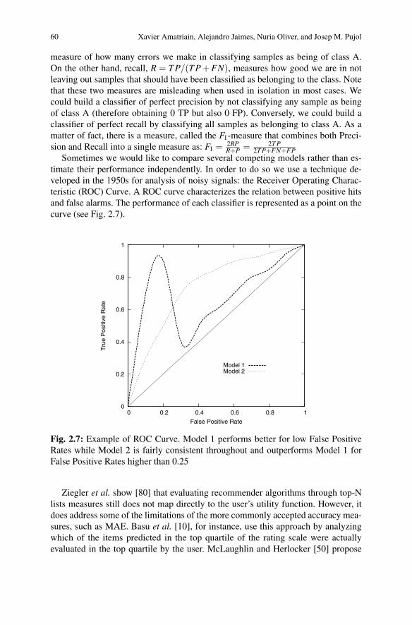
timate their performance independently. In order to do so we use a technique de-veloped in the 1950s for analysis of noisy signals: the Receiver Operating Charac-teristic (ROC) Curve. A ROC curve characterizes the relation between positive hitsand false alarms. The performance of each classifier is represented as a point on thecurve (see Fig. 2.7).

0

0.2

0.4

0.6

0.8

1

0 0.2 0.4 0.6 0.8 1

Tru

e P

ositi

ve R

ate

False Positive Rate

Model 1Model 2

Fig. 2.7: Example of ROC Curve. Model 1 performs better for low False PositiveRates while Model 2 is fairly consistent throughout and outperforms Model 1 forFalse Positive Rates higher than 0.25

Ziegler et al. show [80] that evaluating recommender algorithms through top-Nlists measures still does not map directly to the user’s utility function. However, itdoes address some of the limitations of the more commonly accepted accuracy mea-sures, such as MAE. Basu et al. [10], for instance, use this approach by analyzingwhich of the items predicted in the top quartile of the rating scale were actuallyevaluated in the top quartile by the user. McLaughlin and Herlocker [50] propose


a modified precision measure in which non-rated items are counted as not recom-mendable. This precision measure in fact represents a lower-bound of the “real”precision. Although the F-measure can be directly derived from the precision-recallvalues, it is not common to find it in RS evaluations. Huang et al. [43] and Bozzonet al. [13], and Miyahara and Pazzani [52] are some of the few examples of the useof this measure.

ROC curves have also been used in evaluating RS. Zhang et al. [64] use the valueof the area under the ROC curve as their evaluation measure when comparing theperformance of different algorithms under attack. Banerjee and Ramanathan [8] alsouse the ROC curves to compare the performance of different models.

It must be noted, though, that the choice of a good evaluation measure, even inthe case of a top-N RS, is still a matter of discussion. Many authors have proposedmeasures that are only indirectly related to these traditional evaluation schemes.Deshpande and Karypis [25], for instance, propose the use of the hit rate and theaverage reciprocal hit-rank. On the other hand, Breese et al. [15] define a measureof the utility of the recommendation in a ranked list as a function of the neutral vote.

Note that Chapter 8 details on the use of some of these evaluation measures inthe context of RS and is therefore a good place to continue if you are interested onthis topic.

2.4 Cluster Analysis

The main problem for scaling a CF classifier is the amount of operations involved incomputing distances – for finding the best k-nearest neighbors, for instance. A possi-ble solution is, as we saw in section 2.2.3, to reduce dimensionality. But, even if wereduce dimensionality of features, we might still have many objects to compute thedistance to. This is where clustering algorithms can come into play. The same is truefor content-based RS, where distances among objects are needed to retrieve simi-lar ones. Clustering is sure to improve efficiency because the number of operationsis reduced. However, and unlike dimensionality reduction methods, it is unlikelythat it can help improve accuracy. Therefore, clustering must be applied with carewhen designing a RS, measuring the compromise between improved efficiency anda possible decrease in accuracy.

Clustering [41], also referred to as unsupervised learning, consists of assigningitems to groups so that the items in the same groups are more similar than itemsin different groups: the goal is to discover natural (or meaningful) groups that existin the data. Similarity is determined using a distance measure, such as the onesreviewed in 2.2.1. The goal of a clustering algorithm is to minimize intra-clusterdistances while maximizing inter-cluster distances.

There are two main categories of clustering algorithms: hierarchical and parti-tional. Partitional clustering algorithms divide data items into non-overlapping clus-ters such that each data item is in exactly one cluster. Hierarchical clustering algo-


rithms successively cluster items within found clusters, producing a set of nestedcluster organized as a hierarchical tree.

Many clustering algorithms try to minimize a function that measures the qualityof the clustering. Such a quality function is often referred to as the objective func-tion, so clustering can be viewed as an optimization problem: the ideal clusteringalgorithm would consider all possible partitions of the data and output the partition-ing that minimizes the quality function. But the corresponding optimization problemis NP hard, so many algorithms resort to heuristics (e.g., in the k-means algorithmusing only local optimization procedures potentially ending in local minima). Themain point is that clustering is a difficult problem for which finding optimal solu-tions is often not possible. For that same reason, selection of the particular clusteringalgorithm and its parameters (e.g., similarity measure) depend on many factors, in-cluding the characteristics of the data. In the following paragraphs we describe thek-means clustering algorithm and some of its alternatives.

2.4.1 k-Means

k-Means clustering is a partitioning method. The function partitions the data set ofN items into k disjoint subsets S j that contain N j items so that they are as closeto each other as possible according a given distance measure. Each cluster in thepartition is defined by its N j members and by its centroid λ j. The centroid for eachcluster is the point to which the sum of distances from all items in that cluster isminimized. Thus, we can define the k-means algorithm as an iterative process tominimize E = ∑k

1 ∑n∈S j d(xn,λ j), where xn is a vector representing the n-th item,λ j is the centroid of the item in S j and d is the distance measure. The k-meansalgorithm moves items between clusters until E cannot be decreased further.

The algorithm works by randomly selecting k centroids. Then all items are as-signed to the cluster whose centroid is the closest to them. The new cluster centroidneeds to be updated to account for the items who have been added or removed fromthe cluster and the membership of the items to the cluster updated. This operationcontinues until there are no further items that change their cluster membership. Mostof the convergence to the final partition takes place during the first iterations of thealgorithm, and therefore, the stopping condition is often changed to “until relativelyfew points change clusters” in order to improve efficiency.

The basic k-means is an extremely simple and efficient algorithm. However, itdoes have several shortcomings: (1) it assumes prior knowledge of the data in orderto choose the appropriate k ; (2) the final clusters are very sensitive to the selection ofthe initial centroids; and (3), it can produce empty cluster. k-means also has severallimitations with regard to the data: it has problems when clusters are of differingsizes, densities, and non-globular shapes; and it also has problems when the datacontains outliers.

Xue et al. [77] present a typical use of clustering in the context of a RS by em-ploying the k-means algorithm as a pre-processing step to help in neighborhood for-


mation. They do not restrict the neighborhood to the cluster the user belongs to butrather use the distance from the user to different cluster centroids as a pre-selectionstep for the neighbors. They also implement a cluster-based smoothing technique inwhich missing values for users in a cluster are replaced by cluster representatives.Their method is reported to perform slightly better than standard kNN-based CF. Ina similar way, Sarwar et al. [26] describe an approach to implement a scalable kNNclassifier. They partition the user space by applying the bisecting k-means algorithmand then use those clusters as the base for neighborhood formation. They report adecrease in accuracy of around 5% as compared to standard kNN CF. However, theirapproach allows for a significant improvement in efficiency.

Connor and Herlocker [21] present a different approach in which, instead ofusers, they cluster items. Using the Pearson Correlation similarity measure they tryout four different algorithms: average link hierarchical agglomerative [39], robustclustering algorithm for categorical attributes (ROCK) [40], kMetis, and hMetis 3.Although clustering did improve efficiency, all of their clustering techniques yieldedworse accuracy and coverage than the non-partitioned baseline. Finally, Li et al.[60]and Ungar and Foster [72] present a very similar approach for using k-means clus-tering for solving a probabilistic model interpretation of the recommender problem.

2.4.2 Alternatives to k-means

Density-based clustering algorithms such as DBSCAN work by building up on thedefinition of density as the number of points within a specified radius. DBSCAN,for instance, defines three kinds of points: core points are those that have more thana specified number of neighbors within a given distance; border points have fewerthan the specified number but belong to a core point neighborhood; and noise pointsare those that are neither core or border. The algorithm iteratively removes noisepoints and performs clustering on the remaining points.

Message-passing clustering algorithms are a very recent family of graph-basedclustering methods. Instead of considering an initial subset of the points as centersand then iteratively adapt those, message-passing algorithms initially consider allpoints as centers – usually known as exemplars in this context. During the algorithmexecution points, which are now considered nodes in a network, exchange messagesuntil clusters gradually emerge. Affinity Propagation is an important representativeof this family of algorithms [33] that works by defining two kinds of messagesbetween nodes: “responsibility”, which reflects how well-suited receiving point isto serve as exemplar of the point sending the message, taking into account otherpotential exemplars; and “availability”, which is sent from candidate exemplar to thepoint and reflects how appropriate it would be for the point to choose the candidateas its exemplar, taking into account support from other points that are choosing thatsame exemplar. Affinity propagation has been applied, with very good results, to

3 http://www.cs.umn.edu/ karypis/metis


problems as different as DNA sequence clustering, face clustering in images, or textsummarization.

Finally, Hierarchical Clustering, produces a set of nested clusters organized asa hierarchical tree (dendogram). Hierarchical Clustering does not have to assumea particular number of clusters in advanced. Also, any desired number of clusterscan be obtained by selecting the tree at the proper level. Hierarchical clusters canalso sometimes correspond to meaningful taxonomies. Traditional hierarchical al-gorithms use a similarity or distance matrix and merge or split one cluster at a time.There are two main approaches to hierarchical clustering. In agglomerative hier-archical clustering we start with the points as individual clusters and at each step,merge the closest pair of clusters until only one cluster (or k clusters) are left. Indivisive hierarchical clustering we start with one, all-inclusive cluster, and at eachstep, split a cluster until each cluster contains a point (or there are k clusters).

To the best of our knowledge, alternatives to k-means such as the previous havenot been applied to RS. The simplicity and efficiency of the k-means algorithmshadows possible alternatives. It is not clear whether density-based or hierarchicalclustering approaches have anything to offer in the RS arena. On the other hand,message-passing algorithms have been shown to be more efficient and their graph-based paradigm can be easily translated to the RS problem. It is possible that we seeapplications of these algorithms in the coming years.

2.5 Association Rule Mining

Association Rule Mining focuses on finding rules that will predict the occurrence ofan item based on the occurrences of other items in a transaction. The fact that twoitems are found to be related means co-occurrence but not causality. Note that thistechnique should not be confused with rule-based classifiers presented in Sec. 2.3.3.

We define an itemset as a collection of one or more items (e.g. (Milk, Beer,Diaper)). A k-itemset is an itemset that contains k items. The frequency of a givenitemset is known as support count (e.g. (Milk, Beer, Diaper) = 131). And the supportof the itemset is the fraction of transactions that contain it (e.g. (Milk, Beer, Diaper)= 0.12). A frequent itemset is an itemset with a support that is greater or equal to aminsup threshold. An association rule is an expression of the form X ⇒ Y , whereX and Y are itemsets. (e.g. Milk,Diaper⇒ Beer). In this case the support of theassociation rule is the fraction of transactions that have both X and Y . On the otherhand, the confidence of the rule is how often items in Y appear in transactions thatcontain X .

Given a set of transactions T , the goal of association rule mining is to findall rules having support ≥ minsupthreshold and con f idence≥ mincon f threshold.The brute-force approach would be to list all possible association rules, computethe support and confidence for each rule and then prune rules that do not satisfyboth conditions. This is, however, computationally very expensive. For this reason,we take a two-step approach: (1) Generate all itemsets whose support ≥ minsup


(Frequent Itemset Generation); (2) Generate high confidence rules from each fre-quent itemset (Rule Generation)

Several techniques exist to optimize the generation of frequent itemsets. On abroad sense they can be classified into those that try to minimize the number of can-didates (M), those that reduce the number of transactions (N), and those that reducethe number of comparisons (NM). The most common approach though, is to reducethe number of candidates using the Apriori principle. This principle states that ifan itemset is frequent, then all of its subsets must also be frequent. This is verifiedusing the support measure because the support of an itemset never exceeds that ofits subsets. The Apriori algorithm is a practical implementation of the principle.

Given a frequent itemset L, the goal when generating rules is to find all non-empty subsets that satisfy the minimum confidence requirement. If |L| = k, thenthere are 2k2 candidate association rules. So, as in the frequent itemset generation,we need to find ways to generate rules efficiently. For the Apriori Algorithm we cangenerate candidate rules by merging two rules that share the same prefix in the ruleconsequent.

The effectiveness of association rule mining for uncovering patterns and drivingpersonalized marketing decisions has been known for a some time [2]. However, andalthough there is a clear relation between this method and the goal of a RS, they havenot become mainstream. The main reason is that this approach is similar to item-based CF but is less flexible since it requires of an explicit notion of transaction –e.g. co-occurrence of events in a given session. In the next paragraphs we presentsome promising examples, some of which indicate that association rules still havenot had their last word.

Mobasher et al. [53] present a system for web personalization based on associ-ation rules mining. Their system identifies association rules from pageviews co-occurrences based on users navigational patterns. Their approach outperforms akNN-based recommendation system both in terms of precision and coverage. Smythet al. [68] present two different case studies of using association rules for RS. In thefirst case they use the a priori algorithm to extract item association rules from userprofiles in order to derive a better item-item similarity measure. In the second case,they apply association rule mining to a conversational recommender. The goal hereis to find co-occurrent critiques – i.e. user indicating a preference over a particularfeature of the recommended item. Lin et al. [49] present a new association miningalgorithm that adjusts the minimum support of the rules during mining in order toobtain an appropriate number of significant rule therefore addressing some of theshortcomings of previous algorithms such as the a priori. They mine both associa-tion rules between users and items. The measured accuracy outperforms previouslyreported values for correlation-based recommendation and is similar to the moreelaborate approaches such as the combination of SVD and ANN.

Finally, as already mentioned in section 2.3.2, Cho et al. [18] combine DecisionTrees and Association Rule Mining in a web shop RS. In their system, associa-tion rules are derived in order to link related items. The recommendation is thencomputed by intersecting association rules with user preferences. They look for as-sociation rules in different transaction sets such as purchases, basket placement, and


click-through. They also use a heuristic for weighting rules coming from each of thetransaction sets. Purchase association rules, for instance, are weighted higher thanclick-through association rules.

2.6 Conclusions

This chapter has introduced the main data mining methods and techniques that canbe applied in the design of a RS. We have also surveyed their use in the literatureand provided some rough guidelines on how and where they can be applied.

We started by reviewing techniques that can be applied in the pre-processingstep. First, there is the choice of an appropriate distance measure, which is reviewedin Section 2.2.1. This is required by most of the methods in the following steps.The cosine similarity and Pearson correlation are commonly accepted as the bestchoice. Although there have been many efforts devoted to improving these distancemeasures, recent works seem to report that the choice of a distance function does notplay such an important role. Then, in Section 2.2.2, we reviewed the basic samplingtechniques that need to be applied in order to select a subset of an originally largedata set, or to separating a training and a testing set. Finally, we discussed the useof dimensionality reduction techniques such as Principal Component Analysis andSingular Value Decomposition in Section 2.2.3 as a way to address the curse ofdimensionality problem. We explained some success stories using dimensionalityreduction techniques, especially in the context of the Netflix prize.

In Section 2.3, we reviewed the main classification methods: namely, nearest-neighbors, decision trees, rule-based classifiers, Bayesian networks, artificial neuralnetworks, and support vector machines. We saw that, although kNN ( see Section2.3.1) CF is the preferred approach, all those classifiers can be applied in differentsettings. Decision trees ( see Section 2.3.2) can be used to derive a model basedon the content of the items or to model a particular part of the system. Decisionrules ( see Section 2.3.3) can be derived from a pre-existing decision trees, or canalso be used to introduce business or domain knowledge. Bayesian networks ( seeSection 2.3.4) are a popular approach to content-based recommendation, but canalso be used to derive a model-based CF system. In a similar way, Artificial Neu-ral Networks can be used to derive a model-based recommender but also to com-bine/hybridize several algorithms. Finally, support vector machines ( see Section2.3.6) are gaining popularity also as a way to infer content-based classifications orderive a CF model.

Choosing the right classifier for a RS is not easy and is in many senses task anddata-dependent. In the case of CF, some results seem to indicate that model-basedapproaches using classifiers such as the SVM or Bayesian Networks can slightlyimprove performance of the standard kNN classifier. However, those results are non-conclusive and hard to generalize. In the case of a content-based RS there is someevidence that in some cases Bayesian Networks will perform better than simpler


methods such as decision trees. However, it is not clear that more complex non-linear classifiers such as the ANN or SVMs can perform better.

Therefore, the choice of the right classifier for a specific recommending task stillhas nowadays much of exploratory. A practical rule-of-thumb is to start with thesimplest approach and only introduce complexity if the performance gain obtainedjustifies it. The performance gain should of course balance different dimensionssuch as prediction accuracy or computational efficiency.

We reviewed clustering algorithms in Section 2.4. Clustering is usually used inRS to improve performance. A previous clustering step, either in the user of itemspace, reduces the number of distance computations we need to perform. However,this usually comes at the price of a lower accuracy so it should be handled withcare. As a matter of fact, improving efficiency by using a dimensionality reductiontechnique such as SVD is probably a better choice in the general case. As opposedto what happens with classifiers, not so many clustering algorithms have been usedin the context of RS. The simplicity and relative efficiency of the k-means algorithm(see Section 2.4.1) make it hard to find a practical alternative. We reviewed someof them such as Hierarchical Clustering or Message-passing algorithms in Section2.4.2. Although these techniques have still not been applied for RS, they offer apromising avenue for future research.

Finally, in Section 2.5, we described association rules and surveyed their use inRS. Association rules offer an intuitive framework for recommending items when-ever there is an explicit or implicit notion of transaction. Although there exist effi-cient algorithms for computing association rules, and they have proved more accu-rate than standard kNN CF, they are still not a favored approach.

The choice of the right DM technique in designing a RS is a complex task thatis bound by many problem-specific constraints. However, we hope that the shortreview of techniques and experiences included in this chapter can help the readermake a much more informed decision. Besides, we have also uncovered areas thatare open to many further improvements, and where there is still much exciting andrelevant research to be done in the coming years.

Acknowledgments

This chapter has been written with partial support of an ICREA grant from theGeneralitat de Catalunya.

References

1. Adomavicius, G.,and Tuzhilin, A., Toward the next generation of recommender systems: Asurvey of the state-of-the-art and possible extensions. IEEE Transactions on Knowledge andData Engineering, 17(6):734–749, 2005.


2. Agrawal, R.,and Srikant, R., Fast algorithms for mining association rules in large databases.In Proceedings of the 20th International Conference on Very Large Data Bases, 1994.

3. Amatriain, X., Lathia, N., Pujol, J.M., Kwak, H., and Oliver, N., The wisdom of the few: Acollaborative filtering approach based on expert opinions from the web. In Proc. of SIGIR ’09,2009.

4. Amatriain, X., Pujol, J.M., and Oliver, N., I like it... i like it not: Evaluating user ratings noisein recommender systems. In UMAP ’09, 2009.

5. Amatriain, X., Pujol, J.M., Tintarev, N., and Oliver, N., Rate it again: Increasing recommen-dation accuracy by user re-rating. In Recys ’09, 2009.

6. Anderson, M., Ball, M., Boley, H., Greene, S., Howse, N., Lemire, D., and S. McGrath. Racofi:A rule-applying collaborative filtering system. In Proc. IEEE/WIC COLA’03, 2003.

7. Baets, B.D., Growing decision trees in an ordinal setting. International Journal of IntelligentSystems, 2003.

8. Banerjee, S.,and Ramanathan, K., Collaborative filtering on skewed datasets. In Proc. ofWWW ’08, 2008.

9. Basu, C., Hirsh, H., and Cohen, W., Recommendation as classification: Using social andcontent-based information in recommendation. In In Proceedings of the Fifteenth NationalConference on Artificial Intelligence, pages 714–720. AAAI Press, 1998.

10. Basu, C., Hirsh, H., and Cohen, W., Recommendation as classification: Using social andcontent-based information in recommendation. In AAAI Workshop on Recommender Systems,1998.

11. Bell, R.M., Koren, Y., and Volinsky, C., The bellkor solution to the netflix prize. Technicalreport, AT&T Labs Research, 2007.

12. Bouza, A., Reif, G., Bernstein, A., and Gall, H., Semtree: ontology-based decision tree algo-rithm for recommender systems. In International Semantic Web Conference, 2008.

13. Bozzon, A., Prandi, G., Valenzise, G., and Tagliasacchi, M., A music recommendation sys-tem based on semantic audio segments similarity. In Proceeding of Internet and MultimediaSystems and Applications - 2008, 2008.

14. Brand, M., Fast online svd revisions for lightweight recommender systems. In SIAM Interna-tional Conference on Data Mining (SDM), 2003.

15. Breese, J., Heckerman, D., and Kadie, C., Empirical analysis of predictive algorithms forcollaborative filtering. In Proceedings of the Fourteenth Annual Conference on Uncertainty inArtificial Intelligence, page 4352, 1998.

16. Burke, R., Hybrid web recommender systems. pages 377–408. 2007.17. Cheng, W., J. Huhn, and E. Hullermeier. Decision tree and instance-based learning for label

ranking. In ICML ’09: Proceedings of the 26th Annual International Conference on MachineLearning, pages 161–168, New York, NY, USA, 2009. ACM.

18. Cho, Y., Kim, J., and Kim, S., A personalized recommender system based on web usagemining and decision tree induction. Expert Systems with Applications, 2002.

19. Christakou, C.,and Stafylopatis, A., A hybrid movie recommender system based on neuralnetworks. In ISDA ’05: Proceedings of the 5th International Conference on Intelligent SystemsDesign and Applications, pages 500–505, 2005.

20. Cohen, W., Fast effective rule induction. In Machine Learning: Proceedings of the 12thInternational Conference, 1995.

21. Connor, M.,and Herlocker, J., Clustering items for collaborative filtering. In SIGIR Workshopon Recommender Systems, 2001.

22. Cover, T.,and Hart, P., Nearest neighbor pattern classification. Information Theory, IEEETransactions on, 13(1):21–27, 1967.

23. Cristianini, N.,and J. Shawe-Taylor. An Introduction to Support Vector Machines and OtherKernel-based Learning Methods. Cambridge University Press, March 2000.

24. Deerwester, S., Dumais, S.T., Furnas, G.W., L. T. K., and Harshman, R., Indexing by latentsemantic analysis. Journal of the American Society for Information Science, 41, 1990.

25. Deshpande, M.,and Karypis, G., Item-based top-n recommendation algorithms. ACM Trans.Inf. Syst., 22(1):143–177, 2004.


26. B. S. et al. Recommender systems for large-scale e-commerce: Scalable neighborhood forma-tion using clustering. In Proceedings of the Fifth International Conference on Computer andInformation Technology, 2002.

27. K. O. et al. Context-aware svm for context-dependent information recommendation. In Inter-national Conference On Mobile Data Management, 2006.

28. P. T. et al. Introduction to Data Mining. Addison Wesley, 2005.29. S. G. et al. Tv content recommender system. In AAAI/IAAI 2000, 2000.30. S. H. et al. Aimed- a personalized tv recommendation system. In Interactive TV: a Shared

Experience, 2007.31. T. B. et al. A trail based internet-domain recommender system using artificial neural networks.

In Proceedings of the Int. Conf. on Adaptive Hypermedia and Adaptive Web Based Systems,2002.

32. Freund, Y., Iyer, R., Schapire, R.E., and Singer, Y., An efficient boosting algorithm for com-bining preferences. Mach, J., Learn. Res., 4:933–969, 2003.

33. Frey, B.J.,and Dueck, D., Clustering by passing messages between data points. Science, 307,2007.

34. Friedman, N., Geiger, D., and Goldszmidt, M., Bayesian network classifiers. Mach. Learn.,29(2-3):131–163, 1997.

35. Funk, S., Netflix update: Try this at home, 2006.36. Ghani, R.,and Fano, A., Building recommender systems using a knowledge base of product

semantics. In In 2nd International Conference on Adaptive Hypermedia and Adaptive WebBased Systems, 2002.

37. Goldberg, K., Roeder, T., Gupta, D., and Perkins, C., Eigentaste: A constant time collaborativefiltering algorithm. Journal Information Retrieval, 4(2):133–151, July 2001.

38. Golub, G.,and Reinsch, C., Singular value decomposition and least squares solutions. Nu-merische Mathematik, 14(5):403–420, April 1970.

39. Gose, E., Johnsonbaugh, R., and Jost, S., Pattern Recognition and Image Analysis. PrenticeHall, 1996.

40. Guha, S., Rastogi, R., and Shim, K., Rock: a robust clustering algorithm for categorical at-tributes. In Proc. of the 15th Intl Conf. On Data Eng., 1999.

41. Hartigan, J.A., Clustering Algorithms (Probability & Mathematical Statistics). John Wiley &Sons Inc, 1975.

42. Herlocker, J.L., Konstan, J.A., Terveen, L.G., and Riedl, J.T., Evaluating collaborative filteringrecommender systems. ACM Trans. Inf. Syst., 22(1):5–53, 2004.

43. Huang, Z., Zeng, D., and Chen, H., A link analysis approach to recommendation under sparsedata. In Proceedings of AMCIS 2004, 2004.

44. Isaksson, A., Wallman, M., H. Goransson, and Gustafsson, M.G., Cross-validation and boot-strapping are unreliable in small sample classification. Pattern Recognition Letters, 29:1960–1965, 2008.

45. Jolliffe, I.T., Principal Component Analysis. Springer, 2002.46. Kang, H.,and Yoo, S., Svm and collaborative filtering-based prediction of user preference for

digital fashion recommendation systems. IEICE Transactions on Inf & Syst, 2007.47. Kurucz, M., Benczur, A.A., and Csalogany, K., Methods for large scale svd with missing

values. In Proceedings of KDD Cup and Workshop 2007, 2007.48. Lathia, N., Hailes, S., and Capra, L., The effect of correlation coefficients on communities of

recommenders. In SAC ’08: Proceedings of the 2008 ACM symposium on Applied computing,pages 2000–2005, New York, NY, USA, 2008. ACM.

49. Lin, W.,and Alvarez, S., Efficient adaptive-support association rule mining for recommendersystems. Data Mining and Knowledge Discovery Journal, 6(1), 2004.

50. M. R. McLaughlin and Herlocker, J.L., A collaborative filtering algorithm and evaluationmetric that accurately model the user experience. In Proc. of SIGIR ’04, 2004.

51. S. M. McNee, Riedl, J., and Konstan, J.A., Being accurate is not enough: how accuracy metricshave hurt recommender systems. In CHI ’06: CHI ’06 extended abstracts on Human factorsin computing systems, pages 1097–1101, New York, NY, USA, 2006. ACM Press.


52. Miyahara, K.,and Pazzani, M.J., Collaborative filtering with the simple bayesian classifier. InPacific Rim International Conference on Artificial Intelligence, 2000.

53. Mobasher, B., Dai, H., Luo, T., and Nakagawa, M., Effective personalization based on as-sociation rule discovery from web usage data. In Workshop On Web Information And DataManagement, WIDM ’01, 2001.

54. Nikovski, D.,and Kulev, V., Induction of compact decision trees for personalized recommen-dation. In SAC ’06: Proceedings of the 2006 ACM symposium on Applied computing, pages575–581, New York, NY, USA, 2006. ACM.

55. M. P. Omahony. Detecting noise in recommender system databases. In In Proceedings ofthe International Conference on Intelligent User Interfaces (IUI06), 29th1st, pages 109–115.ACM Press, 2006.

56. Paterek, A., Improving regularized singular value decomposition for collaborative filtering.In Proceedings of KDD Cup and Workshop 2007, 2007.

57. Pazzani, M.J.,and Billsus, D., Learning and revising user profiles: The identification of inter-esting web sites. Machine Learning, 27(3):313–331, 1997.

58. Pronk, V., Verhaegh, W., Proidl, A., and Tiemann, M., Incorporating user control into rec-ommender systems based on naive bayesian classification. In RecSys ’07: Proceedings of the2007 ACM conference on Recommender systems, pages 73–80, 2007.

59. Pyle, D., Data Preparation for Data Mining. Morgan Kaufmann, second edition edition,1999.

60. Li, B., K.Q., Clustering approach for hybrid recommender system. In Web Intelligence 03,2003.

61. Quinlan, J.R., Induction of decision trees. Machine Learning, 1(1):81–106, March 1986.62. Rendle, S.,and L. Schmidt-Thieme. Online-updating regularized kernel matrix factorization

models for large-scale recommender systems. In Recsys ’08: Proceedings of the 2008 ACMconference on Recommender Systems, 2008.

63. Rokach, L., Maimon, O., Data Mining with Decision Trees: Theory and Applications, WorldScientific Publishing (2008).

64. Zhang, J., F.S., Ouyang, Y.,and Makedon, F., Analysis of a low-dimensional linear modelunder recommendation attacks. In Proc. of SIGIR ’06, 2006.

65. Sarwar, B., Karypis, G., Konstan, J., and Riedl, J., Incremental svd-based algorithms forhighly scalable recommender systems. In 5th International Conference on Computer andInformation Technology (ICCIT), 2002.

66. Sarwar, B.M., Karypis, G., Konstan, J.A., and Riedl, J.T., Application of dimensionality re-duction in recommender systemsa case study. In ACM WebKDD Workshop, 2000.

67. Schclar, A., Tsikinovsky, A., Rokach, L., Meisels, A., and Antwarg, L., Ensemble methodsfor improving the performance of neighborhood-based collaborative filtering. In RecSys ’09:Proceedings of the third ACM conference on Recommender systems, pages 261–264, NewYork, NY, USA, 2009. ACM.

68. Smyth, B., K. McCarthy, Reilly, J., D. O‘Sullivan, L. McGinty, and Wilson, D., Case studiesin association rule mining for recommender systems. In Proc. of International Conference onArtificial Intelligence (ICAI ’05), 2005.

69. Spertus, E., Sahami, M., and Buyukkokten, O., Evaluating similarity measures: A large-scalestudy in the orkut social network. In Proceedings of the 2005 International Conference onKnowledge Discovery and Data Mining (KDD-05), 2005.

70. Tiemann, M.,and Pauws, S., Towards ensemble learning for hybrid music recommendation.In RecSys ’07: Proceedings of the 2007 ACM conference on Recommender systems, pages177–178, New York, NY, USA, 2007. ACM.

71. Toescher, A., Jahrer, M., and Legenstein, R., Improved neighborhood-based algorithms forlarge-scale recommender systems. In In KDD-Cup and Workshop 08, 2008.

72. Ungar, L.H.,and Foster, D.P., Clustering methods for collaborative filtering. In Proceedingsof the Workshop on Recommendation Systems, 2000.

73. Witten, I.H.,and Frank, E., Data Mining: Practical Machine Learning Tools and Techniques.Morgan Kaufmann, second edition edition, 2005.


74. Wu, M., Collaborative filtering via ensembles of matrix factorizations. In Proceedings ofKDD Cup and Workshop 2007, 2007.

75. Xia, Z., Dong, Y., and Xing, G., Support vector machines for collaborative filtering. In ACM-SE 44: Proceedings of the 44th annual Southeast regional conference, pages 169–174, NewYork, NY, USA, 2006. ACM.

76. Xu, J.,and Araki, K., A svm-based personal recommendation system for tv programs. InMulti-Media Modelling Conference Proceedings, 2006.

77. Xue, G., Lin,R., Yang, C., Xi, Q., Zeng, W., H.-, Yu, J., and Chen, Z., Scalable collaborativefiltering using cluster-based smoothing. In Proceedings of the 2005 SIGIR, 2005.

78. Yu, K., Tresp, V., and Yu, S., A nonparametric hierarchical bayesian framework for informa-tion filtering. In SIGIR ’04, 2004.

79. Zhang, Y.,and Koren, J., Efficient bayesian hierarchical user modeling for recommendationsystem. In SIGIR 07, 2007.

80. Ziegler, C., McNee N., S. M., Konstan, J.A., and Lausen, G., Improving recommendation liststhrough topic diversification. In Proc. of WWW ’05, 2005.

81. Zurada, J., Introduction to artificial neural systems. West Publishing Co., St. Paul, MN, USA,1992.

Documents

Recommender Systems Handbook || Data Mining Methods for Recommender Systems