Embed Size (px)
Citation preview

ReConAn v1.00 Finite Element Analysis Software
User’s Manual


ReConAn FEA v1.00 – User’s Manual
Aug, 2011 i
ReConAn v1.00 Finite Element Analysis Software
User’s Manual
This manual refers to the ReConAn v1.00 Finite Element Analysis Software.
Developer’s Details:
Assistant Professor George Markou
Faculty member of the Alhosn University of Abu Dhabi, UAE.
Ph.D. NTUA, Department of Civil Engineering, Greece.
email: [email protected]
Place of Development:
The software development took place at the National Technical University of Athens,
Institute of Structural Analysis & Antiseismic Research (ISAAR), Athens
Athens, 2006-2010
© All Rights Reserved

ReConAn FEA v1.00 – User’s Manual
Aug, 2011 ii
This Page was left blank intentionally.

ReConAn FEA v1.00 – User’s Manual
July, 2011 iii
Table of Contents
Table of Figures ........................................................................................................................ v
1. ReConAn v1.00: code features .......................................................................................... 1
2. ReConAn v1.00: code structure ......................................................................................... 3
3. Numerical Methods Incorporated in ReConAn FEA v1.00 .............................................. 9
4. Pre- and Post-processing Environment ............................................................................ 11
5. 2D Linear Analysis with Beam Elements ........................................................................ 13
5.1 Define Material and Property ........................................................................................ 13
5.2 Constructing the Mesh .................................................................................................. 15
5.3 Apply Support Constraints ............................................................................................ 17
5.4 Apply Loads .................................................................................................................. 18
5.5 Set Solution Parameters ................................................................................................ 18
5.6 Export Neutral File ........................................................................................................ 19
5.7 Analysis Procedure ........................................................................................................ 20
5.8 Importing Neutral Output File ....................................................................................... 22
5.9 Graphical Illustration of the Results .............................................................................. 22
6. 2D Nonlinear Analysis with NBCFB Elements .............................................................. 25
6.1 Cantilever Beam with One Material Rectangular Section ............................................ 25
6.2 Cantilever I-Beam (IPE200) .......................................................................................... 28
6.3 Cantilever RC-Beam ..................................................................................................... 30
7. 3D Nonlinear Analysis with NBCFB and Beam Elements ............................................. 35
7.1 Horizontal Loads According to EC8 ............................................................................. 35
7.2 Construction of the FE Mesh ........................................................................................ 37
7.3 Apply Boundary Conditions .......................................................................................... 40
7.3.1 Supports .................................................................................................................. 40
7.3.2 Linear Static Forces ................................................................................................ 41
7.3.3 Nonlinear Horizontal Loads ................................................................................... 42
7.4 Run Analysis and Visualize the Numerical Results ...................................................... 43
8. 3D Analysis with Isoparametric Hexahedral Elements ................................................... 45
8.1 Linear Analysis of a Cantilever Beam .......................................................................... 45
8.1.1 Model with 8-noded Hexahedral Elements ............................................................ 45

ReConAn FEA v1.00 – User’s Manual
July, 2011 iv
8.1.2 Model with 20-noded Hexahedral Elements .......................................................... 50
8.2 Nonlinear Analysis with Hexahedral Elements............................................................. 53
8.2.1 Model with 8-noded Hexahedral Elements ............................................................ 53
8.2.2 Model with 20-noded Hexahedral Elements .......................................................... 56
9. Detailed 3D Modeling of Reinforced Concrete Structures .............................................. 59
9.1 Simply Supported RC Beam ......................................................................................... 59
9.1.1 Models with 8-noded Hexahedral and Rod Elements ............................................ 60
9.1.2 Models with 20-noded Hexahedral and Rod Elements .......................................... 72
9.1.3 Models with 8-noded Hexahedral and NBCFB Elements ...................................... 73
9.2 RC Frame with Shear Wall ........................................................................................... 75
10. Hybrid Modeling (HYMOD) ........................................................................................... 81
10.1 Cantilever Steel Beam ................................................................................................. 82
10.2 RC Frame .................................................................................................................... 85
References ............................................................................................................................... 87

ReConAn FEA v1.00 – User’s Manual
July, 2011 v
Table of Figures
Chapter 4
Figure 4.1 Main window of Femap FEA with SMAD custom properties. ............................. 11
Chapter 5
Figure 5.1 Cantilever beam with rectangular section. ............................................................ 13
Figure 5.2 Defining a material. ............................................................................................... 14
Figure 5.3 Defining a beam property. ..................................................................................... 15
Figure 5.4 Defining the section of the beam. .......................................................................... 15
Figure 5.5 Defining the FE and its section’s orientation. ....................................................... 16
Figure 5.6 FE mesh with (a) 1 and (b) 10 elements. ............................................................... 16
Figure 5.7 SMAD custom properties tool. .............................................................................. 16
Figure 5.8 Custom properties for the case of the Beam FE. ................................................... 17
Figure 5.9 Create a constraint set. ........................................................................................... 17
Figure 5.10 Assign constraints. ............................................................................................... 18
Figure 5.11 Create load sets. ................................................................................................... 18
Figure 5.12 Final FE model with a single beam element. ...................................................... 18
Figure 5.13 Set Analysis parameters. ..................................................................................... 19
Figure 5.14 Export Femap neutral file. ................................................................................... 19
Figure 5.15 Dialog Box of Femap. Export neutral file notifications for the case of the single
beam element mesh. ............................................................................................. 20
Figure 5.16 Dialog Box of ReConAn FEA v1.00. .................................................................. 20
Figure 5.17 Dialog Box of ReConAn FEA v1.00 after the completion of the analysis. ........ 21
Figure 5.18 (a) Importing a Femap neutral file and (b) Dialog box Import Neutral File
confirmation. ........................................................................................................ 22
Figure 5.19 Deformed shapes of the cantilever beam discretized with (Up) one and (Down)
ten beam finite elements. ........................................................................................................ 22
Chapter 6
Figure 6.1 Change the custom properties of the Beam element into the NBCFB’s element. 25
Figure 6.2 Updating the nonlinear analysis parameters. ......................................................... 26
Figure 6.3 P-δ curve for a total vertical load of 100 kN. ........................................................ 27
Figure 6.4 Complete plastification of a rectangular section. .................................................. 27
Figure 6.5 P-δ curve of the cantilever beam. .......................................................................... 28
Figure 6.6 FE mesh of the I-beam cantilever. ......................................................................... 28
Figure 6.7 Property definition (Left). Shape definition of the I cross section (Right). .......... 29
Figure 6.8 Custom properties definition for the case of an I-beam. ....................................... 29
Figure 6.9 Custom properties definition for the case of an I-beam. ....................................... 30
Figure 6.10 Numerically predicted P-δ curve for the case of the I-beam. .............................. 30
Figure 6.11 Geometry and reinforcement details of a cantilever RC beam.[2]
........................ 31

ReConAn FEA v1.00 – User’s Manual
July, 2011 vi
Figure 6.12 Discretization of the rectangular RC section with fibers.[2]
................................. 31
Figure 6.13 Custom properties definition for the case of a RC beam. .................................... 32
Figure 6.14 Numerically predicted P-δ curve for the case of the RC beam. .......................... 33
Chapter 7
Figure 7.1 2-storey RC framed structure. ............................................................................... 35
Figure 7.2 Reinforcement details of the cross sections. .......................................................... 35
Figure 7.3 Custom properties of the three RC fiber cross sections. ........................................ 38
Figure 7.4 FE mesh. Columns of the 1st storey and shear wall with rigid element. ............... 39
Figure 7.5 FE mesh. (Left) Columns, shear wall and beams of the 1st storey. (Right) Finite
elements with offset and diaphragm (rigid elements in red color). ........................ 39
Figure 7.6 FE mesh of the 2-storey RC structure. (Left) 3D Frame. (Right) Finite elements
with offset and diaphragm (rigid elements in red color). ....................................... 40
Figure 7.6 FE mesh of the 2-storey RC structure. Fix constraints at the base nodes of the
model. ..................................................................................................................... 40
Figure 7.8 Creating a load set named “LoadStatic”. ............................................................... 41
Figure 7.9 Activating body loads along the negative Z-axis direction. .................................. 42
Figure 7.10 Static loads distributed at each nodal beam. A total vertical load of 198.2 kN. .. 42
Figure 7.11 Nonlinear parameters. .......................................................................................... 42
Figure 7.12 Horizontal seismic loads. ..................................................................................... 43
Figure 7.13 Computed deformed shape at load-step 25. ......................................................... 43
Figure 7.14 P-δ curves for 25 and 50 Newton-Raphson load steps. ....................................... 44
Chapter 8
Figure 8.1 Discretization with 8-noded hexahedral elements (2x5x30). ................................ 46
Figure 8.2 Hexahedral property definition. ............................................................................. 46
Figure 8.3 Material definition. ................................................................................................ 47
Figure 8.4 SMAD custom properties for the case of hexahedral elements. ............................ 47
Figure 8.5 Cantilever beam’s FE model. Discretized with hexahedral elements. .................. 47
Figure 8.6 Analysis parameters for the case of a single load step solution scheme. .............. 48
Figure 8.7 Time file for the case of the cantilever beam with 8-noded hexahedral elements. 48
Figure 8.8 Deformed shape of the cantilever beam. ............................................................... 49
Figure 8.9 Output vectors that can be visualized graphically. ................................................ 49
Figure 8.10 Deformed shape and von Mises stress contour. .................................................. 50
Figure 8.11 von Mises stress contour. Dynamic cut along the plane YZ. .............................. 50
Figure 8.12 Executing the Linear/Parabolic Order command. ............................................... 51
Figure 8.13 Updated hexahedral mesh (300 20-noded hexahedral elements, 1935 modes). .. 51
Figure 8.14 Deformed shape of the cantilever beam. 20-noded hexahedral elements. .......... 52
Figure 8.15 Time file for the case of the cantilever beam with 20-noded hexahedral elements.
.............................................................................................................................. 52
Figure 8.16 Hexahedral mesh of a RC cantilever beam supported on a shear wall. ............... 53
Figure 8.17 Editing of the material parameters....................................................................... 54
Figure 8.18 Editing the Nonlinear Analysis parameters. ........................................................ 55

ReConAn FEA v1.00 – User’s Manual
July, 2011 vii
Figure 8.19 Yielding initiation. Von Mises stress contour. .................................................... 55
Figure 8.20 Von Mises stress contour prior complete plastification. ..................................... 55
Figure 8.21 20-noded hexahedral mesh. ................................................................................. 56
Figure 8.22 P-δ curve. 20-noded hexahedral mesh. ................................................................ 56
Figure 8.23 Deformed shape prior to failure. 20-noded hexahedral mesh. ............................ 57
Figure 8.24 Shear wall-beam joint. Deformed shape prior to failure of the (a) upper and (b)
lower sectional areas. ........................................................................................... 57
Figure 8.25 TIME.dat file for the case of the 20-noded hexahedral mesh (50 load increments).
.............................................................................................................................. 58
Chapter 9
Figure 9.1 Simply supported RC beam. Geometry and reinforcement details. ...................... 59
Figure 9.2 Define concrete material C25/30. .......................................................................... 60
Figure 9.3 Define steel material S500. .................................................................................... 61
Figure 9.4 Mesh construction of the beam. ............................................................................. 61
Figure 9.5 Beam’s hexahedral mesh with metallic plates at the supports. ............................. 62
Figure 9.6 Rebar property definitions. A-B. Fi8 and C-D. Fi20. ............................................ 64
Figure 9.7 Custom properties of Hexa8_C25 (concrete hexahedral elements). ..................... 64
Figure 9.8 Custom properties of Fi8 and Fi20 reinforced properties. .................................... 65
Figure 9.9 Construction process of the embedded rebar mesh. .............................................. 67
Figure 9.10 Supports (Left) Pin and (Right) Roller. ............................................................... 67
Figure 9.11 Concentrate vertical forces on the mid-span of the beam (240 kN). ................... 68
Figure 9.12 Defining nonlinear analysis parameters. ............................................................. 68
Figure 9.13 Deformed shape and crack pattern prior to failure (P = 336 kN). ....................... 69
Figure 9.14 P-δ curve of the simply supported beam. Steel hardening modulus equal to 2.1
GPa. ...................................................................................................................... 69
Figure 9.15 P-δ curve of the simply supported beam. Steel hardening modulus equal to zero.
.............................................................................................................................. 69
Figure 9.16 ReConAn Eye main command window. ............................................................. 70
Figure 9.17 ReConAn DOS window. Entering the load increment number. ......................... 71
Figure 9.18 Crack pattern inside the beam. Load increment 33. ............................................ 71
Figure 9.19 FE mesh with metallic plates at support and loading areas. ................................ 71
Figure 9.20 Crack pattern prior to failure. FE mesh with metallic plates at support and
loading areas. ....................................................................................................... 72
Figure 9.21 Required computational time for the nonlinear analysis of 18 load increments. 72
Figure 9.22 Crack pattern prior to failure. 20-noded hexahedral FE mesh with metallic plates
at support and loading areas. ................................................................................ 72
Figure 9.23 P-δ curve of 8-noded and 20-noded hexahedral elements. Simply supported
beam with steel hardening modulus equal to zero. .............................................. 73
Figure 9.24 Deformed shape of the embedded rebar elements prior to failure. 20-noded
hexahedral FE mesh with metallic plates at support and loading areas. .............. 73
Figure 9.25 Custom properties of Fi20 with NBCFB embedded element attributes. ............. 74
Figure 9.26 Comparison of P-δ curves of the simply supported beam. Steel hardening
modulus equal to zero. ......................................................................................... 74

ReConAn FEA v1.00 – User’s Manual
July, 2011 viii
Figure 9.27 RC frame. Geometric features and reinforcement details. .................................. 75
Figure 9.28 RC frame with shear wall. 8-noded hexahedral discretization. ........................... 76
Figure 9.29 RC frame with shear wall. Initial embedded rebar elements. .............................. 76
Figure 9.30 Custom properties of Fi22 with NBCFB embedded element attributes. ............. 77
Figure 9.31 RC frame with shear wall. P-δ curve. .................................................................. 77
Figure 9.32 Crack pattern and deformed shape prior to failure A. XZ view and B. 3D view 78
Figure 9.33 RC frame with shear wall. von Mises strain contour prior to failure. A. 37th
and
B. 38th
load increments. ........................................................................................ 79
Figure 9.34 RC frame with shear wall. Numerical error and required internal iterations per
each load increment. ............................................................................................. 80
Chapter 10
Figure 10.1 Discretization of joints with detailed solid and beam elements. Reinforcement
details and fiber discretization of the beam-column sections[2]
. .......................... 81
Figure 10.2 RC Frame. Discretization schemes with different levels of model reduction[2]
. . 81
Figure 10.3 Cantilever beam. Hybrid FE mesh with A. 8-noded and B. 20-noded hexahedral
elements. ............................................................................................................... 82
Figure 10.4 Cantilever beam. Hybrid FE mesh construction procedure. ................................ 84
Figure 10.5 Rigid element definition. ..................................................................................... 84
Figure 10.6 Cantilever beam. Deformed shapes of the A. 8-noded and B. 20-noded Hybrid
FE models............................................................................................................. 85
Figure 10.7 RC frame. FE meshes. ......................................................................................... 85
Figure 10.8 RC frame. P-δ curves. .......................................................................................... 86

ReConAn FEA v1.00 – User’s Manual
Sep, 2011 Page 1
1. ReConAn v1.00: code features
It is well known that every FEM program consists of three different parts. The first
and the third parts are those that deal with the visualization of the FEM model and the
results that the second part produces. Meaning that we have a pre– and post– processing
program (first and third part respectively) for the creation (mesh generators, renumbering
etc.) and visual illustration of FEM arithmetic models (nodes, elements, material etc.) and
results (stress, strain, displacements etc.). For the arithmetic analysis procedure we need a
FEM solver which is the one responsible for the interpretation of the FEM mesh geometry
into the final arithmetical model which will be solved by using the required solution
strategy. After the arithmetic interpretation, the FEM solver will use the appropriate
solution procedure in order to generate the required results through the solution of the
model. For the creation and the visual representation of ReConAn FEM models, an
interface was developed that gives ReConAn the ability to read all required FEM
information from a neutral text type file that Femap v9.0 produce.
Femap provides comprehensive functionality in an independent environment for
modeling, simulation and review of product performance results. Geometry creation;
Import or export of several file types; Meshing; User interface; Results; API.
ReConAn uses two post-processing programs. The first one is Femap, which provides all
necessary post-processing tools that a FEM code should have, such as stress and strain
contouring, virtual animation etc. The second post-processing program is ReConAn Eye
which is encapsulated inside ReConAn main code structure. ReConAn Eye is based on
pre-build OpenGL libraries f90gl. f90gl is a public domain implementation of the
official Fortran 90 bindings for OpenGL. OpenGL is the industry's most widely used,
supported and best documented 2D/3D graphics API making it inexpensive & easy to
obtain information on implementing OpenGL in hardware and software. The need for the
creation of a second post-processor lied within the inability of Femap to illustrate
discontinuities (cracks). One of the material models that ReConAn includes in its material
libraries, is that of the 3D smeared crack material model. The smeared crack approach
gives the arithmetic ability of modeling materials that are dominated by crack phenomena
such as concrete. Due to the fact that Femap cannot illustrate 3D cracks at a Finite
Elements gauss point, the development of a visual tool that could do so was necessary.
ReConAn Eye has the ability of 3D crack visualization in addition to its basic abilities
(3D graphical FEM model illustration, deformations - animation).
The generic code of ReConAn is written in Fortran 90/95 language and the development
was done with the use of Microsoft Visual Studio. The latest Intel Fortran Compiler was

ReConAn FEA v1.00 – User’s Manual
Sep, 2011 Page 2
used for the build of the final product (Release Configuration). ReConAn FEA v1.00 was
built to run in Windows XP, Vista and 7 for 32bit and 64bit CPU systems.
ReConAn code requires further numerical testing in order to configure its numerical
advantages in correlation with other software packages. Nevertheless, all numerical
research that were conducted for this reason, showed that ReConAn combines numerical
robustness and efficiency.

ReConAn FEA v1.00 – User’s Manual
Sep, 2011 Page 3
2. ReConAn v1.00: code structure
During the development of ReConAn software, the necessity for the creation of a more
general in-core object oriented analysis code immersed. This necessity was out driven from
the fact that Finite Element Analysis codes should be easily extendable and preservable
(reusability). In addition to that, from the developers’ site of view, in order to be able to
control the numerical procedures and to have the ability to check the results produced during
the analysis phase, the structure of the code must have object oriented architecture.
Object-oriented programming (OOP) can trace its roots to the 1960s. As hardware and
software became increasingly complex, quality was often compromised. Researchers studied
ways in which software quality could be maintained. Object-oriented programming was
deployed in part as an attempt to address this problem by strongly emphasizing discrete units
of programming logic and re-usability in software. Computer programming methodology
focuses on data rather than processes, with programs composed of self-sufficient modules
(objects) containing all the information needed within its own data structure for manipulation.
Object-oriented programming may be seen as a collection of cooperating objects, as opposed
to a traditional view in which a program may be seen as a group of tasks to compute
("subroutines"). In OOP, each object is capable of receiving messages, processing data, and
sending messages to other objects. Each object can be viewed as an independent little
machine with a distinct role or responsibility. The actions or "operators" on the objects are
closely associated with the object. For example, in object oriented programming, the data
structures tend to carry their own operators around with them (or at least "inherit" them from
a similar object or "class"). The traditional approach tends to view and consider data and
behavior separately.
The development of an OOP type FEM code has many advantages such as the control of
the arithmetic flow which is a rather difficult task as the code is growing and the enrichment
of the code with new Finite Elements, Analysis Procedures, Solvers and other arithmetic
tools that can be encapsulated very fast (extendibility). Taking under consideration the above
code development strategy, ReConAn has adopted this philosophy and has all the pre
mentioned abilities. The outcome from the adoption of this code architectural type is the
evolution of ReConAn into a general FEM program that is able to use several Finite
Elements, Material Models and Solution Procedure.
Object oriented format requires the use of Data Types where for every element, material,
property, solution variables etc. we create a different Data Type. This way, each finite
element has its own property type that tells us which material model it will use during the
solution procedure and its characteristics. Therefore, two different types of elements can use
the same material model or vice-versa. Material variables have their own data types which
are used to store data that refer to material characteristics like the Young Modulus, Poisson

ReConAn FEA v1.00 – User’s Manual
Sep, 2011 Page 4
Ratio etc. Property data type contain information about each element and its characteristics
concerning the material model that this element is going to use during the analysis procedure,
the Integration Method that the stiffness procedure will use for the stiffness matrix creation
etc.
Finite Element programming can be considered by many users as a straight forward job
and it does not require any sophisticated code language. In reality this is partially true. Even
the smallest in size Finite Element simulations require a certain number of arithmetical
operations between two dimensional matrices and arrays. These matrix operations require a
certain amount of time in order to be carried out, accordingly to the number of unknowns at
hand. This means the bigger a FEM model is the more computational time and virtual
memory is required in order to be solved. Designing with FEM the last 3 decades and the
need for more accuracy in simulations, led Engineers to simulate their structures with finer
meshes and large number of nodes. CPU hardware ability enhancements were the main
reason that Engineering computational analysis had and still have an upper boundary limit
concerning the models size. This need for large scale simulations led towards two different
concepts, parallel processing and optimum dynamic usage of CPU hardware abilities through
optimum code programming. If we would like to take this question, which concept should
we be adopting; the answer would not be straight forward. The optimum choice would be a
combination of these two concepts in order to have the optimum code structure and
architecture which will lead to the optimum performance.
In order to have an optimum code structure, firstly we must choose the adequate
programming language which will provide us the necessary tools in order to create an
optimally designed code for the problems at hand. Taking under consideration the above
remarks (about the FEM arithmetical nature), one could easily say that we need a
programming language which will be able to dynamically redistribute CPU virtual memory
and handle optimally large arithmetic matrix (arrays) operations.
In computer science, dynamic memory allocation is the allocation of memory storage for
use in a computer program during its runtime. It can be seen also as a way of distributing
ownership of limited memory resources among many pieces of data and code. Dynamically
allocated memory exists until it is released either explicitly by the programmer, exiting a
block, or by the garbage collector. This is in contrast to static memory allocation, which has
a fixed duration. It is said that an object that is allocated has a dynamic lifetime (allocate -
deallocate). Programming languages like Java, Visual Basic, Pascal, Matlab, Apple etc. have
the ability of memory dynamic allocation and object oriented programming but they are
deficient in speed due to their inability in handling large arithmetic operations. This problem
immersed from the fact that the creators of these programming languages in order to make
them more user friendly they included many invisible intermediate operations that reduced
significantly the operations speed during the runtime. The best choices for our problem at
hand are C++ (or C#) and Fortran 90/95.
C++ and C# are used widely by many developers but Fortran 77 and the new Fortran
90/95 due to its simpler language style always dominated in the scientific research field in

ReConAn FEA v1.00 – User’s Manual
Sep, 2011 Page 5
terms of preference. Fortran 77 is considered to be rather “old” and antiquated since the new
features of Fortran 90/95 language were introduced.
The much delayed successor to FORTRAN 77, informally known as Fortran 90, was
finally released as an ISO standard in 1991 and an ANSI Standard in 1992. This major
revision added many new features to reflect the significant changes in programming practice
that had evolved since the 1978 standard:
Free-form source input, also with lowercase Fortran keywords
Identifiers up to 31 characters in length
Inline comments
Ability to operate on arrays (or array sections) as a whole, thus greatly simplifying
math and engineering computations.
whole, partial and masked array assignment statements and array expressions,
such as
X (1:N) = R (1:N) * COS (A (1:N)))
WHERE statement for selective array assignment
array-valued constants and expressions,
user-defined array-valued functions and array constructors.
RECURSIVE procedures
Modules, to group related procedures and data together making them available to
other program units, including the capability to limit the accessibility only to specific
parts of the module.
A vastly improved argument-passing mechanism, allowing interfaces to be checked
at compile time
User-written interfaces for generic procedures
Operator overloading
Derived/abstract data types
New data type declaration syntax, to specify the data type and other attributes of
variables
Dynamic memory allocation by means of the ALLOCATABLE attribute and the
ALLOCATE and DEALLOCATE statements
POINTER attribute, pointer assignment and NULLIFY statement to facilitate the
creation and manipulation of dynamic data structures
Structured looping constructs, with an END DO statement for loop termination, and
EXIT and CYCLE statements for "breaking out" of normal DO loop iterations in an
orderly way
SELECT . . . CASE construct for multi-way selection
Portable specification of numerical precision under the user's control
New and enhanced intrinsic procedures.
Unlike the previous revision, Fortran 90 did not delete any features. (Appendix B.1 says,
"The list of deleted features in this standard is empty.") Any standard-conforming
FORTRAN 77 program is also standard-conforming under Fortran 90 and either standard
should be usable to define its behavior.
A small set of features were identified as "obsolescent" and expected to be removed in a
future standard.

ReConAn FEA v1.00 – User’s Manual
Sep, 2011 Page 6
Obsolescent feature Example Status /
95
Arithmetic IF-statement IF (X) 10, 20, 30
Non-integer DO parameters or control
variables
DO 9 X= 1.7, 1.6, -0.1 Deleted
Shared DO-loop termination or
termination with a statement
other than END DO or CONTINUE
DO 9 J= 1, 10
DO 9 K= 1, 10
9 L= J + K
Branching to END IF
from outside a block
66 GO TO 77 ; . . .
IF (E) THEN ; . . .
77 END IF
Deleted
Alternate return CALL SUBR( X, Y *100, *200 )
PAUSE statement PAUSE 600
Deleted
ASSIGN statement
and assigned GO TO statement
100 . . .
ASSIGN 100 TO H
. . .
GO TO H . . .
Deleted
Assigned FORMAT specifiers ASSIGN F TO 606
Deleted
H edit descriptors 606 FORMAT ( 9H1GOODBYE. )
Deleted
Computed GO TO statement GO TO (10, 20, 30, 40), index
(Obso.)
Statement functions FOIL( X, Y )= X**2 + 2*X*Y +
Y**2 (Obso.)
DATA statements
among executable statements
X= 27.3
DATA A, B, C / 5.0, 12.0. 13.0
/. . .
(Obso.)
CHARACTER* form of CHARACTER
declaration
CHARACTER*8 STRING ! Use
CHARACTER(8) (Obso.)
Assumed character length functions
Fixed form source code
* Column 1 contains * or ! or C for
comments.
C Column 6 for continuation.
Table 2.1 Obsolescent features of Fortran 77.

ReConAn FEA v1.00 – User’s Manual
Sep, 2011 Page 7
Fortran 95 was a minor revision, mostly to resolve some outstanding issues from the
Fortran 90 standard. Nevertheless, Fortran 95 also added a number of extensions, notably
from the High Performance Fortran specification:
FORALL and nested WHERE constructs to aid vectorization
User-defined PURE and ELEMENTAL procedures
Pointer initialization and structure default initialization.
A number of intrinsic functions were extended (i.e. a dim argument was added to the
maxloc intrinsic). Several features noted in Fortran 90 to be deprecated were removed from
Fortran 95:
REAL and DOUBLE PRECISION DO variables
Branching to an END IF statement from outside its block
PAUSE statement
ASSIGN and assigned GOTO statement and assigned format specifiers
H edit descriptor.
An important supplement to Fortran 95 was the ISO technical report TR-15581:
Enhanced Data Type Facilities, informally known as the Allocatable TR. This specification
defined enhanced use of ALLOCATABLE arrays, prior to the availability of fully Fortran
2003-compliant Fortran compilers. Such uses include ALLOCATABLE arrays as derived
type components, in procedure dummy argument lists and as function return values.
(ALLOCATABLE arrays are preferable to POINTER-based arrays because
ALLOCATABLE arrays are guaranteed by Fortran 95 to be deallocated automatically when
they go out of scope, eliminating the possibility of memory leakage. In addition, aliasing is
not an issue for optimization of array references, allowing compilers to generate faster code
than in the case of pointers). Another important supplement to Fortran 95 was the ISO
technical report TR-15580: Floating-point exception handling, informally known as the
IEEE TR. This specification defined support for IEEE floating-point arithmetic and floating
point exception handling.
One of the most important features that Fortran 90/95 introduced was the ability to use
pure procedures and array assignments. For example if someone wants to allocate, initialize
and contact some arithmetical operation with a real double precision array that has a size of
iSize, then there are two ways to go with this. The first way is by using the standard do …
enddo format and the second is by using assignments and pure procedures.
do…enddo command Assignments and Pure Procedures
do I = 1, iSize
raArray (I) = 2.d0
raArray (I) = raArray (I)+ abs(raArray
(I) -
(raArray (I) * (-16.d0))) + 4.d0 * raArray
(I) –
(raArray (I) **(1.d0/3.d0))
enddo
raArray (1:iSize) = 2.d0
raArray = raArray + abs(raArray - (raArray
* (-16.d0))) + 4.d0 * raArray – (raArray
**(1.d0/3.d0))
Table 2.2 Example of assignments and pure procedures.
ReConAn FEA v1.00 – User’s Manual
Sep, 2011 Page 8
The first thing that comes to our attention just by looking at these two code formats is
that when assignments and pure procedures are used the code becomes automatically more
compact and it requires half of the lines that do…enddo format has. The second thing that we
achieve by using these new features is that the array elements assignment is not done directly
by using the standard do…enddo way which means that the compiler can optimize the code
by using the optimum assignment numbering. The third advantage of this language format is
that there is no need for creating additional zero subroutines. Zero subroutines were used in
order to initialize a certain array (set it equal to zero).
Another choice that the developer has to make is that of choosing the appropriate
Compiler that the developer program will use in order to convert the text written code into
machine language. Since we chose as our programming language Fortran 90/95 the choices
reduce to the latest and more advanced Fortran Compiler.
Intel® Fortran Compiler Professional Edition offers the best support for creating multi-
threaded applications. Only the Professional Edition offers the breadth of advanced
optimization, multi-threading, and processor support that includes automatic processor
dispatch, vectorization, auto-parallelization, OpenMP, data prefetching, loop unrolling,
substantial Fortran 2003 support and an optimized math processing library. The Professional
Edition combines a high performance compiler, which now includes support for Debian and
Ubuntu, with Intel® Math Kernel Library (Intel® MKL). While this library is available
separately, the Professional Edition creates a strong foundation for building robust, high
performance parallel code.
Finally, since we’ve made all the choices concerning the programming language and
compile/build procedures, we need to choose a suitable developing program which will
provide us the necessary developing and debugging tools in order to make the codes
developing task easier and controllable. The most advanced developing studio that
uses .NET technology is considered to be Visual Studio 2008 Professional Edition (SP1).
Visual Studio 2008 Professional Edition is a comprehensive set of tools that accelerates
the process of turning the developer’s vision into reality. Visual Studio 2008 Professional
Edition was engineered to support development projects that target the Web (including
ASP.NET AJAX), Windows Vista, Windows Server 2008, 2007 Microsoft Office system,
SQL Server 2008 and Windows Mobile devices. Visual Studio 2008 Professional Edition
provides the integrated toolset for addressing all the developer’s needs by providing a
superset of the functionality available in Visual Studio 2008 Standard Edition. In addition to
that, Visual Studio 2008 Professional Edition can create Fortran console applications. This is
done by simply installing the Intel® Fortran Compiler Professional Edition after the
installation of Visual Studio 2008 Professional Edition. By doing this, Visual Studio 2008
Professional Edition adds in its Project Types an additional one named Intel(R) Fortran.

ReConAn FEA v1.00 – User’s Manual
Sep, 2011 Page 9
3. Numerical Methods Incorporated in ReConAn FEA v1.00
Material Library
1. Bilinear Steel Material Model (1D, Static Nonlinear Analysis)
2. Menegotto & Pinto Steel Material Model with kinematic hardening (1D, Static Nonlinear
Analysis)
3. Kent & Park Concrete Material Model (1D, Static Nonlinear Analysis)
4. Von Misses Consistent Material Model (3D, Static Nonlinear Analysis)
5. Smeared Crack Material Models (3D, Static Nonlinear Analysis)
6. Soil Material Models (will be included in ReConAn v2.00)
Element Library
1. 3D 2noded Beam Element (12 degrees of freedom)
2. 3D 2noded Beam Column Element (BEC) with fiber approach and natural shapes
3. 3D 2noded Natural Beam-Column Force-Based Element (NBCFB) with fiber approach
and natural shapes
4. 3D 8noded Isoparametric Hexahedral Element
5. 3D 20noded Isoparametric Hexahedral Element
6. 3D 3noded Triangular Shell Element TRIC (will be included in ReConAn v2.0)
Problem Solution Library
1. Static Linear Analysis
2. Static Non-Linear Analysis (Newton-Raphson with force- and displacement control, Arc-
Length with Large Displacements)
3. Dynamic Linear Analysis (will be included in ReConAn v2.00)
4. Dynamic Non-Linear Analysis (will be included in ReConAn v2.00)
Solver Library
1. Gauss Elimination using Skyline Storage
2. Preconditioned Conjugated Gradient (PCG) using Compact Storage
(i: No Preconditioning, ii: Diagonal Preconditioning, iii: SSOR Preconditioning)

ReConAn FEA v1.00 – User’s Manual
Sep, 2011 Page 10

ReConAn FEA v1.00 – User’s Manual
Sep, 2011 Page 11
4. Pre- and Post-processing Environment
Visual illustration of the FE model and the corresponding results after the completion of
an analysis, is one of the most essential features of a FEA code for the following basic
reasons:
1. Create and check the geometry of the FE model.
2. Set or modify the material and analysis parameters.
3. Represent visually the output data in order to verify the correctness of the computed
results during the analysis procedure.
When dealing with relatively large models, the use of user friendly post-processing
software is imperative for assessing the quality of the FE models. Many researchers use text
type input file to provide the necessary information regarding the FE geometry, material
properties and analysis details. Furthermore, the usual output that results from this type of
analysis is restrained to monitoring the displacement along a specific direction of a node. It is
obvious that this leads to many uncertainties which increase as the FE increases in terms of
the dof number.
Figure 4.1 Main window of Femap FEA with SMAD custom properties.
For the above reasons, ReConAn FEA has been supplemented with the ability of reading
the required FE geometry and features from a Femap[1]
neutral file and exporting its output
data in a text file which can be imported in Femap post-processing software utilizing the user
with the ability of illustrating visually the deformations and several contour options of the
resulted stresses and strains. Additionally, ReConAn Eye post-processing software was
developed during this Dissertation so as to visualize the predicted crack patterns when the
smeared modeling command was activated. This software is OpenGL based and has the
ReConAn FEA v1.00 – User’s Manual
Sep, 2011 Page 12
ability of animating the evolution of cracking during the load history analysis of a RC
structure. The necessity of developing such a tool emerges from the fact that Femap post-
processing software does not provide the ability of crack representation, thus all figures of
this research work containing crack patterns were taken from ReConAn Eye post-processing
software.
Since Femap pre-processing software does not provide the user with the necessary tools
for entering custom made properties regarding several features of the FE models (like the
number of fibers per control section in the case of the NBCFB element), the SMAD Custom
properties software (Fig. 7.1) was used for providing any additional parameters required by
the ReConAn solver for the assemblage and solution of the numerical problem at hand. The
SMAD Custom properties software was developed by G. Stavroulakis during his Ph.D.
Thesis, which deals with soil-structure interaction problems under seismic loading with the
use of the FEM.

ReConAn FEA v1.00 – User’s Manual
Sep, 2011 Page 13
5. 2D Linear Analysis with Beam Elements
This numerical implementation will present the complete procedure of modeling,
analyzing and graphically representing the output of a single cantilever beam which is loaded
with a concentrated force at the tip (Fig. 5.1).
Figure 5.1 Cantilever beam with rectangular section.
In order to analyze this cantilever beam, the meshing of the structural member is
performed after the material definition. It is important to say here that the construction of a
finite element (FE) model follows the exact same procedure with that executed when the
Femap FEA is used for both modeling and analysis. When ReConAn is used for the analysis,
Femap is used as the pre- and post-processing tool through which the material, mesh and
analysis data are defined. The procedure that a user should follow so as to ensure that the
derived model will be correctly read by the ReConAn FEA software is the following:
I. Define materials.
II. Define properties.
III. Assign custom properties through SMAD.
IV. Create the mesh.
V. Define constraint sets. Then assign constraints.
VI. Define load sets. Then assign loads.
VII. Define Nonlinear Parameters.
VIII. Check for coincident nodes or elements (this does not apply for HYBRID models).
IX. Renumber nodes and elements.
X. Export neutral file in 9.0 version.
XI. Analyze with ReConAn FEA.
XII. Import results into Femap.
Each one of these steps will be presented analytically through this numerical example.
The construction of any other FE model follows the same procedure thus, for obvious
reasons, when presenting the rest of the numerical implementations we will focus only on the
differences that may apply on the above steps when dealing with new analysis or model
types.
5.1 Define Material and Property
Defining a material in Femap is very simple since its graphical environment is user-
friendly and the execution of its several commands simple. At this point it should be
mentioned that in this User’s Manual the Femap v10.1.1 is used. The users can construct

ReConAn FEA v1.00 – User’s Manual
Sep, 2011 Page 14
their models by using any version above v9.0. Through the main menu, the Model menu is
selected and the Material command is activated. The window in Fig. 5.2 appears where the
material properties are defined. For the case of the Beam FE, the only material properties are
defined directly through the SMAD custom properties tool, therefore in this case the material
is created so as to be able to create the corresponding beam property as it will be shown next.
Figure 5.2 Defining a material.
The most important thing that a user should always have in mind before starting the
definition of any property, are the units of the values that ReConAn uses during the analysis
procedure. All values must be given as plain number and the same unit system must be used
throughout the model. If the users decides to use MPa when defining the Young modulus
parameter (30,000 MPa = 30 GPa), then all values that refer to forces, other Young moduli,
yielding stresses, etc. should be defined in MN or MPa. Furthermore, since MPa = MN / m2,
all geometrical features should be defined in meters (m). If the FE mesh is constructed by
adopting the assumption that 1 unit in Femap equals to 1 cm and at the same time the Young
modulus is defined in kPa, then the computations will derive results that will not reflect the
desired numerical model.
The unit system that was adopted throughout this manual is the SI and specifically when
defining forces we use kN, when defining stresses kPa and for distances the unit of meters is
used. The next step is to define, through the use of the same menu list, the beam property. By
executing Model Property, the window of Fig. 5.3 appears where the different parameters
of the beam property can be set. For the case of the Beam element, the user has to choose the
Element/Property Type of Beam and press OK. Then, by pressing Shape, the definition of
the Rectangular Bar section has to be performed, where the height and width of the section
are set (Fig. 5.4). After drawing the section (define Height and Width, then press draw), the
OK button is pressed where all the required geometrical features of the section are being
computed. After the assignment of the name and the material that this property will use
during the numerical computations, the property definition is finalized by pressing OK.

ReConAn FEA v1.00 – User’s Manual
Sep, 2011 Page 15
Figure 5.3 Defining a beam property.
Figure 5.4 Defining the section of the beam.
5.2 Constructing the Mesh
The mesh of the FE model can be constructed by using all the tools provided in the
graphical environment of Femap. For this case it is chosen to construct 2 different meshes,
where the discretization assumes one and ten beam elements, respectively. The discretization
of the two meshes can be seen in Figs. 5.6a and 5.6b. It is important to note here that the
graphical illustration abilities of Femap does not provide the user with the ability to visualize
the curvature of the beam element, regardless the fact that the formulation of the beam and
during the computations all 12 degrees of freedom (dof) are accounted for, thus the bending
of the element is considered.

ReConAn FEA v1.00 – User’s Manual
Sep, 2011 Page 16
After creating the ending nodes of the first model (Model Node) the Model
Element command is executed so as to construct the beam element. As it can be seen in Fig.
5.5, the nodes of the element are required and the Vector orientation has to be defined. For
all beam finite elements that ReConAn incorporates, the Method that the user has to apply is
the Vector Global Axis (Fig. 5.5 second window). After the user’s method selection the
Direction has to be specified. In this case, we select Positive and Y Axis, since the cantilever
beam is assumed to have its longitudinal axis along the global x axis (Figs 5.6). Fig. 5.4
shows the local axis of the beam’s section. The y local axis is always parallel to the vector
specified through the “Vector Global Axis – Define Orientation Vector” window. This way
the user can specify the 3D section orientation in space.
Figure 5.5 Defining the FE and its section’s orientation.
(a) (b)
Figure 5.6 FE mesh with (a) 1 and (b) 10 elements.
The next step is to customize all the properties. This is done through the use of the
SMAD custom properties tool which is shown in Fig. 5.7. The custom properties are divided
into four general groups: a. Beam Fiber, b. Beam, c. Hexa and d. Reinforcement property.
For this numerical implementation, we double click on the property named Beam25x50 and
the Beam property is selected while the required fields are being assigned with the
appropriate values, as shown in Fig. 5.8. The value assignment is performed by double
clicking on the boxes located at the Value column (Fig. 5.8) and after the assignment
completion the Apply button has to be pressed.
Figure 5.7 SMAD custom properties tool.

ReConAn FEA v1.00 – User’s Manual
Sep, 2011 Page 17
Figure 5.8 Custom properties for the case of the Beam FE.
Fig. 5.8 shows the different parameters and flags that need to be specified. The “Type of
section” flag can only be equal to 1 since for this type of FE the section must be rectangular.
Additional sections will be available to the user in a future version of ReConAn FEA. The
“Steel Material” parameter that refers to the material model used during the analysis can be
set either to Bilinear or Menegotto & Pinto (1 or 2, respectively). Nevertheless, since this FE
incorporates a linear formulation the above material models are used to compute the elastic
stress that derives from the computed elastic strain at the beam’s section level. For this
reason the “Steel Hardening” and “Steel Fy” parameters, which refer to the hardening ration
and the yielding stress of the beam, respectively, are set to zero.
5.3 Apply Support Constraints
The next step is to create a constraint set (Fig. 5.9) and apply the boundary conditions
according to the support system of the structure’s idealized model. Each node of the beam
FE has 6 dofs thus the user can fix any dof or apply any constraint combination by fixing a a
single, a group or all the dofs of a node.
Figure 5.9 Create a constraint set.

ReConAn FEA v1.00 – User’s Manual
Sep, 2011 Page 18
Figure 5.10 Assign constraints.
As it is shown in Fig. 5.10, the TX, TY and TZ refer to the translational dofs and the RX,
RY and RZ refer to the rotational dofs along the x, y and z global axis, respectively. Given
the fact that the cantilever beam (Fig. 5.1) has its left node fixed, node 1 of both models
(Figs. 5.6a and 5.6b) are fully constrained.
5.4 Apply Loads
ReConAn FEA v1.00 has the ability of accounting for static linear and static nonlinear
concentrated forces / moments. Body loads are also accounted for when the corresponding
command is activated through the Model Load Body. For this numerical
implementation it is assumed that a static vertical concentrated load (100 kN) is applied at
the tip of the cantilever beam. In order to assign the concentrated load it is required to create
a load set by executing Model Load Create/Manage Set. A name is assigned to the new
load set and the procedure is finalized by pressing Done. Then, by executing Model Load
Nodal.
Figure 5.11 Create load sets.
Figure 5.12 Final FE model with a single beam element.
5.5 Set Solution Parameters
ReConAn is able to read all the required solution parameters from the Model Load
Nonlinear Analysis or Dynamic Analysis commands, thus the user has to specify the desired

ReConAn FEA v1.00 – User’s Manual
Sep, 2011 Page 19
analysis type and set the corresponding values. For the case of the static linear analysis, the
Nonlinear Analysis is selected and the number of Increments is set to 1. This implies that the
load will be applied in a single load increment. More analytical description on the Nonlinear
parameters of Fig. 5.13 will be presented at a later stage.
Figure 5.13 Set Analysis parameters.
It is notable to say that these parameters apply to the Load Set that was created so as to
incorporate the loads assigned at each node. There are cases where the load sets are more
than one, therefore when executing the Nonlinear Analysis command the proper Load Set
needs to be activated. This will ensure that the reading procedure will be performed
according to the user’s specifications and for the case of a nonlinear analysis, the nonlinear
parameters will be grouped with the proper load assignments.
5.6 Export Neutral File
The final step before executing the analysis is to export the Femap Neutral file, as shown
in Fig. 5.14. After executing File Export Femap Neutral, a window appears that
requires the specification of the file’s name and then the Neutral File Write Options appears
(Fig. 5.14). In this window the user must select only the Write Analysis Model and Minimize
File Size options and the 9.0 Version from the corresponding list. Then press OK.
Figure 5.14 Export Femap neutral file.
ReConAn FEA v1.00 – User’s Manual
Sep, 2011 Page 20
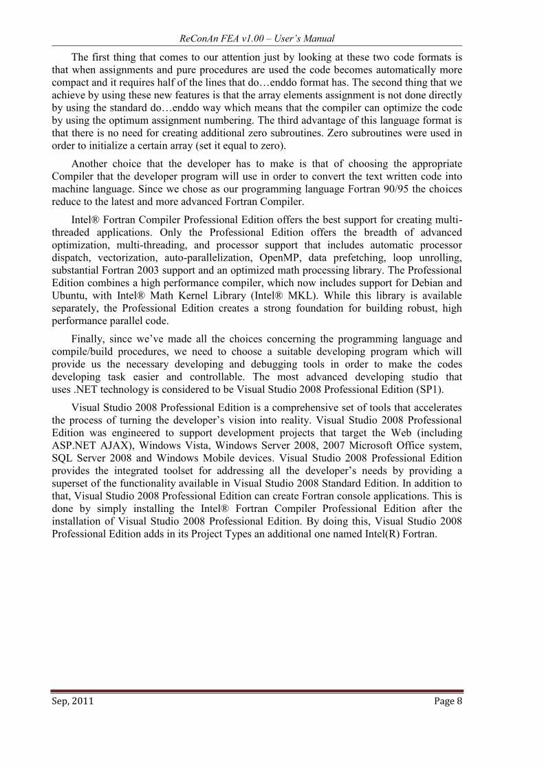
After the proper execution of the above export procedure, Femap will notify you that the
required data were exported and written in the neutral file successfully. The expected
notifications can be seen in Fig. 5.15, located in the corresponding dialog box of Femap.
Before moving to the next step, it is important to note that the name of the neutral file must
not include any spaces.
Figure 5.15 Dialog Box of Femap. Export neutral file notifications for the case of the single
beam element mesh.
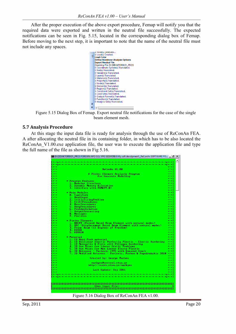
5.7 Analysis Procedure
At this stage the input data file is ready for analysis through the use of ReConAn FEA.
A after allocating the neutral file in its containing folder, in which has to be also located the
ReConAn_V1.00.exe application file, the user was to execute the application file and type
the full name of the file as shown in Fig 5.16.
Figure 5.16 Dialog Box of ReConAn FEA v1.00.

ReConAn FEA v1.00 – User’s Manual
Sep, 2011 Page 21
After typing or copy/paste the neutral file name, the next step is to press enter and the
analysis proceeds automatically. The user can read different type of warnings and
confirmation messages during the reading/initialization/solution/output procedures. Due to
the software’s optimum code design, this is feasible only when the FE models are relatively
large. For the case of this numerical model the software manages to execute all the above
procedures in less than a second. Therefore, for reading any messages the user has to scroll
the window so as to see the different notifications as they are illustrated in Figs. 5.17.
Figure 5.17 Dialog Box of ReConAn FEA v1.00 after the completion of the analysis.

ReConAn FEA v1.00 – User’s Manual
Sep, 2011 Page 22
5.8 Importing Neutral Output File
The completion of the analysis procedure is followed by the creation of the neutral
output file which contains all the output data regarding the displacements and deformations
of the FE model. The file name is the same with that of the input file containing at the end
the “_OUT” word. If the name “1ElementCantileverBeam.NEU” was assigned to the input
file, then ReConAn will automatically name the output file as
“1ElementCantileverBeam_OUT.NEU”. After executing the import command, as it is shown
in Fig. 5.18, the resulted data are now available for visual illustration in Femap.
(a) (b)
Figure 5.18 (a) Importing a Femap neutral file and (b) Dialog box Import Neutral File
confirmation.
5.9 Graphical Illustration of the Results
Femap post-processing graphical environment has many illustrational tools, which are
available to the user so as to visualize the resulted output data after the analysis completion.
Fig. 5.19a and 5.19b shows the deformed shapes of the cantilever beam when discretized
with 1 and 10 beam elements respectively. As it was mentioned previously, Femap does not
have the ability of visualizing the rotation of a single beam element thus the single FE beam
mesh appears as a straight line. This is not the case though since the derived vertical tip
displacement is the same to that computed form the 10 beam element FE mesh (0.0115 m).
Figure 5.19 Deformed shapes of the cantilever beam discretized with (Up) one and (Down) ten beam
finite elements.
Before moving to the next numerical implementation, it is necessary to state here that
even though a 2D analysis was executed, the user is not asked to constraint the dofs that
produce translations outside the cantilever’s plane (TY, RX, RZ), ReConAn managed to
solve this problem as a 2D numerical case without the need of applying any additional

ReConAn FEA v1.00 – User’s Manual
Sep, 2011 Page 23
constraints. If the user wants to constraint the TY, RX, RZ dofs, the only thing that has to be
additionally performed is to apply the above dofs constraints on the nodes that are not
considered to be fixed.

ReConAn FEA v1.00 – User’s Manual
Sep, 2011 Page 24

ReConAn FEA v1.00 – User’s Manual
Sep, 2011 Page 25
6. 2D Nonlinear Analysis with NBCFB Elements The Natural Beam-Column Forced-Based element incorporates several numerical
techniques described analytically in the Ph.D. Thesis[2]
of Markou G. (2011). The main
numerical techniques that this advanced FE incorporates are the fiber approach, which is
used to discretize each section of the beam, the natural mode method for describing the
beam’s deformations and the flexibility (or force) method for computing the stiffness matrix
of each NBCFB element.
The goal here is to discretized the cantilever beam of Fig. 5.1 with one NBCFB element
and analyze this structural member be executing a Push Over analysis with ReConAn. Since
the construction of the model follows exactly the same procedure, the only steps from the
previous numerical implementation, that require modification, are the Custom Property and
the Nonlinear Parameter definition (sections 5.1 and 5.5, respectively). After discretizing and
analyzing by assuming that the cantilever beam has a rectangular section, the same model
will be used while a steel I-beam section will be assigned to the model.
6.1 Cantilever Beam with One Material Rectangular Section
The fastest way to go is to copy/paste the existing neutral input file
(1ElementCantileverBeam.NEU) and rename it into “1ElementCantileverNBCFB.NEU”. By
double clicking on the new input file, the numerical model opens in Femap where the pre-
mentioned modifications are performed.
Figure 6.1 Change the custom properties of the Beam element into the NBCFB’s element.
Fig. 6.1 shows that by changing the custom properties group of the existing Beam25x50
property, from “Beam” to “Beam Fiber” (left window of Fig. 6.1), the custom properties
change and a new set of parameters need to be defined. For the case of the NBCFB element,
the Type of section determines whether the beam is considered to have a homogenous
material (steel) or is a RC beam. Section types 1 and 2 represent to a rectangular one material
and an I beam one material cases, thus section type 3 refers to the rectangular RC section.
For the needs of this numerical implementation, the section type 1 is selected since we

ReConAn FEA v1.00 – User’s Manual
Sep, 2011 Page 26
consider that the cantilever beam will be assumed to have a homogenous material behavior
(like steel) but its material characteristics will be those of concrete (E = 30 GPa, ν = 0.2, fc =
30 MPa and material hardening H = 0). Given the fact that the section type 1 is used and the
Menegotto & Pinto material model is selected (Steel Material = 2), the only parameters that
require being field are those of:
i. Number of fibers (this is the number that ReConAn will use so as to discretize
each section)
ii. Type of section (1: Rectangular Steel, 2: I-Beam, 3: Rectangular RC))
iii. Steel Young Modulus
iv. Poisson Ratio
v. Steel Hardening
vi. Steel Fy (Yielding Stress)
vii. iNumberOfIntegrPoints (Number of Gauss-Lobato integration points, which are
the number of control sections along the element’s longitudinal axis)
viii. Steel Material (material numerical model)
ix. Material (material flag to specify if this is a steel or a RC beam)
x. Type of Fiber Element (1: NBCFB, 2: BEC)
Do not forget to press Apply after the modification of the values. The next modification
that is required to be performed is that of the Nonlinear Analysis parameters. Through the
Model Load Nonlinear Analysis command the corresponding window is opened and
the load increments are changed from 1 to 50 (Fig. 6.2). The internal iterations per load
increment (Max Iterations / Step) is set to 25 and the number of iterations before executing a
stiffness matrix update is set to 1 (Iterations Before Update), thus the stiffness matrix is
updated at each internal iteration when plastification occurs. Finally, the Convergence
Tolerance is set to Work 10-4
which is a sufficient value for ensuring an acceptable
robustness and accuracy during the nonlinear solution procedure.
Figure 6.2 Updating the nonlinear analysis parameters.
The final step before executing the Push Over analysis is to export the new neutral input
file through the same procedure presented in section 5.6. By executing the ReConAn
application file, typing the new input file name and by pressing the enter button, ReConAn
performs all the required numerical procedures so as to read, initialize, solve and write the
output file. After the successful completion of the analysis, the import of the resulted output
file is performed as described in section 5.8 and the graphical illustration of the deformed
shape and the time-history deformation can be viewed. Furthermore, the P-δ curve can be

ReConAn FEA v1.00 – User’s Manual
Sep, 2011 Page 27
exported as described in Femap user’s manual. Fig. 6.3 shows the resulted curve, where it
can be seen that the beam behaves elastically.
The next step is to increase the vertical load in order to observe nonlinear mechanical
behavior due to the material properties degradation (when yielding occurs) and eventually
compute the maximum load that can be applied prior to failure. Fig. 6.4 shows the schematic
representation of a completely plastification of a rectangular section.
Figure 6.3 P-δ curve for a total vertical load of 100 kN.
Figure 6.4 Complete plastification of a rectangular section.
The analytical failure load is PP = 156.4 kN which can be computed through the use of
the following equations:
,P P PM F h where 2
iP y i
hF f b 6.1
PP
MP
L
6.2
Since the analytical failure load is known, the existing load is modified through the
Modify Edit Load Individual from 100 kN to 160 kN so as to exceed the computed
failure load. As it can be seen from Fig. 6.5, the analytically computed failure load coincides
with the load predicted by the FE model with the NBCFB element and 100 Newton-Raphson
load increments (Fig. 6.5). Since the formulation of this element adopts the Euler-Bernoulli
theory of the undeformed section, the analytical solution coincides with the numerical that
results from the combination of the FE method and the fiber approach. For the case of the 50
Newton-Raphson increments the solution procedure is terminated at a total load of 153.6 kN
which corresponds to the total load at load increment 48. When the nonlinear solution
0
20
40
60
80
100
120
0 0.5 1 1.5
Tip Displacement (cm)
Load
P (
kN)

ReConAn FEA v1.00 – User’s Manual
Sep, 2011 Page 28
proceeds to load increment 49, the total applied load equals to 49/50*160 = 156.8 kN which
is larger than the analytically computed failure load thus the cantilever beam fails and the
numerical procedure cannot convergence. This shows the importance of choosing the
appropriate load increment when dealing with nonlinear numerical implementations and the
role that this parameter has when trying to interpret the derived numerical results.
Figure 6.5 P-δ curve of the cantilever beam.
6.2 Cantilever I-Beam (IPE200)
The easiest way to modify and convert the previous cantilever beam by changing its section
into an IPE200 steel section is by creating a new beam property and re-assign the proper
parameters regarding the material and geometry of the section. The FEM model is shown in
Fig. 6.6 where the section of the FE is shown in 3D. The material model used in this
numerical experiment is the Menegotto – Pinto with Young modulus, tangent modulus and
yield stress equal to: E = 200 GPa, Et = 2 GPa and fy = 235 MPa, respectively.
In order to modify the rectangular section of the cantilever beam, the creation of a new
property is performed, as shown in Fig. 6.7, and the corresponding custom properties
parameters are being assigned as shown in Fig. 6.8. Thereafter, the command Modify
Update Elements Property ID (Fig. 6.9) has to be executed in order to change the current
property from Beam25x50 to IPE200. As it can be seen in Fig. 6.6, the vertical concentrated
load on the tip of the cantilever is set to 30 kN. The modification of the applied load can be
performed through the Modify Edit Load - Individual command.
Figure 6.6 FE mesh of the I-beam cantilever.

ReConAn FEA v1.00 – User’s Manual
Sep, 2011 Page 29
Figure 6.7 Property definition (Left). Shape definition of the I cross section (Right).
Figure 6.8 Custom properties definition for the case of an I-beam.

ReConAn FEA v1.00 – User’s Manual
Sep, 2011 Page 30
Figure 6.9 Custom properties definition for the case of an I-beam.
The numerically predicted mechanical behavior of the cantilever beam can be depicted
in Fig. 6.10 which illustrated the derived P-δ curve. As it can be seen the resulted curve
shows that the cantilever behaves elastically up to a load of 17 kN where nonlinearities occur
thus the plastification of the section initiates. After the complete plastification of the section
the stiffness of the cantilever beam is control by the hardening modulus which is equal to 2
GPa. The inclination of the curve’s metelastic branch is 100 times less than that of the elastic
branch, a numerical phenomenon that derives from the relations between the elastic Young
modulus and the hardening modulus (200 GPa and 2 GPa, respectively).
Figure 6.10 Numerically predicted P-δ curve for the case of the I-beam.
6.3 Cantilever RC-Beam
The last numerical implementation presented in this Chapter is that of a RC cantilever
beam with a vertical concentrated force applied in the tip. The same procedure is followed as
presented in Section 6.2, where the FE mesh is modified accordingly. For the needs of this

ReConAn FEA v1.00 – User’s Manual
Sep, 2011 Page 31
numerical example, the FE mesh of the Section 6.1 is used as a starting point, while the
geometrical features of the section and the reinforcement details that are going to be
implemented can be depicted in Fig. 6.11. ReConAn incorporates an automatic mesh-
generator for discretizing the cross section of a rectangular RC beam with fibers (Fig. 6.12).
Additional shapes will be considered in future versions. The required data for the meshing
procedure are the number of fibers (including the rebar fibers), the concrete cover, the
number of longitudinal reinforcement on the upper/lower/side of the section and the stirrups
(diameter and spacing). A typical discretization with fibers is shown in Fig. 6.12, where it
can be seen that the section is divided into two areas: a. the unconfined and b. the confined
area. These two areas are identified automatically by the mesh procedure thus the proper
material model is assigned and used during the numerical analysis. ReConAn incorporates
the Kent & Park[4]
material model for concrete, which takes into account the confinement
effect and for the steel material the bilinear and Menegotto & Pinto[5]
material model.
Figure 6.11 Geometry and reinforcement details of a cantilever RC beam.
[2]
Figure 6.12 Discretization of the rectangular RC section with fibers.
[2]
After opening the input file created in Section 6.1 (rectangular section cantilever beam)
the custom properties are modified so as to account for the RC material features. The
modifications can be seen in Fig. 6.13, where it must be noted that the steel material model
selected was the Menegotto & Pinto. The parameter “Flag Reb Put” has to do with the way
that rebar fibers are created. If this parameter is set to 1 then additional fibers are created for
modeling the reinforcement while when is set to 0 then existing concrete fibers are being
replaced by reinforcement. It is recommended to set this parameter equal to 1 since this
approach is proved to be numerically robust. Furthermore, if the user choses to use the
second approach then the number of fibers used for the discretization of the section has to be
large enough in order to assure that there is a sufficient number of concrete fibers so as to be
replaced by the number of longitudinal reinforcement. If the user sets the number of fibers to

ReConAn FEA v1.00 – User’s Manual
Sep, 2011 Page 32
10 then the number of fibers inside the confined upper area of the section will be two. If the
number of longitudinal reinforcement is 3 then the replacement procedure cannot proceed. In
addition to that the area of these two concrete fibers will much larger than the rebar area thus
the numerical implementation will result into unrealistic output.
Figure 6.13 Custom properties definition for the case of a RC beam.
Fig. 6.13 shows the selected custom properties parameters for the case of the cantilever RC
beam. The material characteristics that were used for the concrete material model were: Ec =
30 GPa and fc = 30 MPa, (Young modulus and compressive strength, respectively). The
corresponding material characteristics of the reinforcing steel bars were: Es = 210 GPa, Et =
2.1 GPa, fy = 500 MPa and hc = 0.03 m, where E, Et, fy and hc are the Young modulus, the
tangent modulus, the yielding stress and the concrete cover width, respectively. The Flag
Reb Put parameter is set to 1 and the rebar diameter to 20 mm. Note that the diameter has to
be given in mm as requested by the custom properties parameter name “rRebDiamDow
(mm)”. The “rHoopDiam (mm)” refers to the stirrup diameter in mm while the
“rHoopDistance (cm)” and “rHoopFy (MPa)” are the constant distance in centimeters
between stirrups and the yielding stress of the stirrups reinforcement in MPa, respectively.
The “RC Conf Material Model” and “RC UnConf Material Model” are always set to 3 and 4,
respectively, and they are used as material flags when the Kent & Park material model is
used during the nonlinear analysis procedure. It is reminded to press Apply after the
completion of the parameter definition so as to finalize all the applied modifications.
Before exporting the updated input file, the vertical applied concentrated force is
modified and set equal to 100 kN. The nonlinear procedure is executed and the resulted P-δ
curve is given in Fig. 6.14.

ReConAn FEA v1.00 – User’s Manual
Sep, 2011 Page 33
Figure 6.14 Numerically predicted P-δ curve for the case of the RC beam.

ReConAn FEA v1.00 – User’s Manual
Sep, 2011 Page 34

ReConAn FEA v1.00 – User’s Manual
Sep, 2011 Page 35
7. 3D Nonlinear Analysis with NBCFB and Beam Elements This chapter presents the ability of ReConAn to model 3D structures and combine the
two different beam finite elements incorporated in its FE library. To serve this purpose, the
2-storey 3D frame is considered (Fig. 7.1) for nonlinear analysis according to the EC8[3]
. For
simplicity reasons the distributed loads will be accounted for as concentrated gravity forces
applied at the structure’s beams. In addition to that, the direction that will be investigated is
only the global x-axis which is the direction where the horizontal loads will be applied.
Therefore, the next step is to compute the horizontal loads, and then construct the FE mesh
according to the idealized model shown in Fig. 7.1. The procedure of constructing the mesh
will be also presented in detail so as to illustrate the way that ReConAn accounts for
different modeling feature (i.e. diaphragm, offsets, static dead loads, etc.).
Figure 7.1 2-storey RC framed structure.
Figure 7.2 Reinforcement details of the cross sections.
7.1 Horizontal Loads According to EC8
The assumed EC8 parameters are given in Table 7.1 and the procedure for computing
the base shear force due to the design seismic excitation can be depicted in Table 7.2.
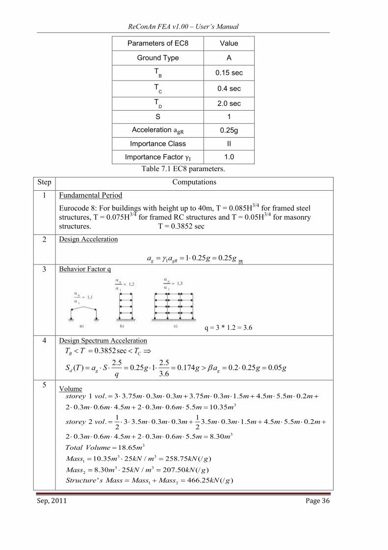
ReConAn FEA v1.00 – User’s Manual
Sep, 2011 Page 36
Parameters of EC8 Value
Ground Type Α
TB 0.15 sec
TC 0.4 sec
TD 2.0 sec
S 1
Acceleration 0.25g
Importance Class II
Importance Factor 1.0
Table 7.1 EC8 parameters.
Step Computations
1 Fundamental Period
Eurocode 8: For buildings with height up to 40m, T = 0.085H3/4
for framed steel
structures, T = 0.075H3/4
for framed RC structures and T = 0.05H3/4
for masonry
structures. T = 0.3852 sec
2 Design Acceleration
1 0.25 0.25g gRa a g g
3 Behavior Factor q
q = 3 * 1.2 = 3.6
4 Design Spectrum Acceleration
5 Volume
0.3852sec
2.5 2.5( ) 0.25 1 0.174 0.2 0.25 0.05
3.6
B C
d g g
T T T
S T a S g g a g gq
3
1 . 3 3.75 0.3 0.3 3.75 0.3 1.5 4.5 5.5 0.2
2 0.3 0.6 4.5 2 0.3 0.6 5.5 10.35
1 1 2 . 3 3.5 0.3 0.3 3.5 0.3 1.5 4.5 5.5 0.2
2 2
2 0.3 0.6 4.5 2 0.3 0.6 5
storey vol m m m m m m m m m
m m m m m m m
storey vol m m m m m m m m m
m m m m m
3
3
3 3
1
3 3
2
1 2
.5 8.30
18.65
10.35 25 / 258.75 (/ )
8.30 25 / 207.50 (/ )
' 466.25 (/ )
m m
Total Volume m
Mass m kN m kN g
Mass m kN m kN g
Structure s Mass Mass Mass kN g
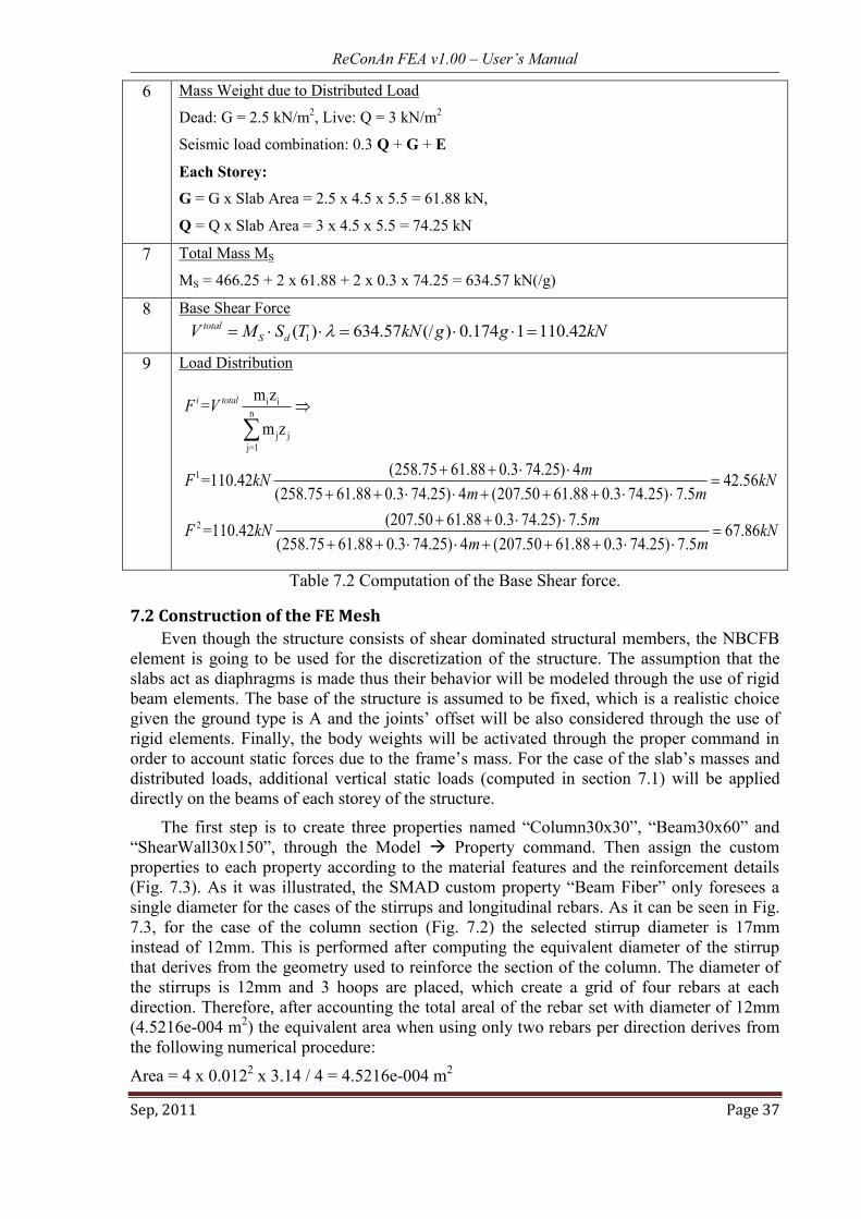
ReConAn FEA v1.00 – User’s Manual
Sep, 2011 Page 37
6 Mass Weight due to Distributed Load
Dead: G = 2.5 kN/m2, Live: Q = 3 kN/m
2
Seismic load combination: 0.3 Q + G + E
Each Storey:
G = G x Slab Area = 2.5 x 4.5 x 5.5 = 61.88 kN,
Q = Q x Slab Area = 3 x 4.5 x 5.5 = 74.25 kN
7 Total Mass MS
MS = 466.25 + 2 x 61.88 + 2 x 0.3 x 74.25 = 634.57 kN(/g)
8 Base Shear Force
9 Load Distribution
Table 7.2 Computation of the Base Shear force.
7.2 Construction of the FE Mesh
Even though the structure consists of shear dominated structural members, the NBCFB
element is going to be used for the discretization of the structure. The assumption that the
slabs act as diaphragms is made thus their behavior will be modeled through the use of rigid
beam elements. The base of the structure is assumed to be fixed, which is a realistic choice
given the ground type is A and the joints’ offset will be also considered through the use of
rigid elements. Finally, the body weights will be activated through the proper command in
order to account static forces due to the frame’s mass. For the case of the slab’s masses and
distributed loads, additional vertical static loads (computed in section 7.1) will be applied
directly on the beams of each storey of the structure.
The first step is to create three properties named “Column30x30”, “Beam30x60” and
“ShearWall30x150”, through the Model Property command. Then assign the custom
properties to each property according to the material features and the reinforcement details
(Fig. 7.3). As it was illustrated, the SMAD custom property “Beam Fiber” only foresees a
single diameter for the cases of the stirrups and longitudinal rebars. As it can be seen in Fig.
7.3, for the case of the column section (Fig. 7.2) the selected stirrup diameter is 17mm
instead of 12mm. This is performed after computing the equivalent diameter of the stirrup
that derives from the geometry used to reinforce the section of the column. The diameter of
the stirrups is 12mm and 3 hoops are placed, which create a grid of four rebars at each
direction. Therefore, after accounting the total areal of the rebar set with diameter of 12mm
(4.5216e-004 m2) the equivalent area when using only two rebars per direction derives from
the following numerical procedure:
Area = 4 x 0.0122 x 3.14 / 4 = 4.5216e-004 m
2
1( ) 634.57 (/ ) 0.174 1 110.42total
S dV M S T kN g g kN
i i
n
j j
j=1
1
2
m z=
m z
(258.75 61.88 0.3 74.25) 4=110.42 42.56
(258.75 61.88 0.3 74.25) 4 (207.50 61.88 0.3 74.25) 7.5
(207.50 61.88 0.3 74.25) 7.5=110.42
(258.75 61.88 0.3 74.25) 4 (207.5
i totalF V
mF kN kN
m m
mF kN
m
67.860 61.88 0.3 74.25) 7.5
kNm

ReConAn FEA v1.00 – User’s Manual
Sep, 2011 Page 38
2 x Dequiv.2 π / 4 = 4.5216e-004. Dequiv. = (2 x 4.5216e-004 / π)
0.5 = 0.017 m = 17mm
It is important to note at this point that shear reinforcement is taken into account through
the K coefficient that is used in the Kent & Park concrete material model so as to include the
increase in the compressive strength due to confinement.
1 ,
s y hoop
c c
c
fK f K f
f
K is a factor which takes account for the strength increase due to confinement, cf is the
concrete compressive cylinder strength in MPa, y hoopf is the yield strength of stirrups in MPa
and ρs is the ratio of the volume of hoop reinforcement to the volume of concrete core
measured outside of stirrups.
Figure 7.3 Custom properties of the three RC fiber cross sections.
The next step is to create the rigid element property and define the proper parameters so
as to create a practically undeformable FE. This is performed by creating a beam property
named “BeamRigid” and assigning a very large value for the Young modulus parameter. For
the needs of this numerical implementation it was chosen to set E = 10,000 GPa and the
section’s geometry was set to be equal to 40x40cm. As it was discussed previously, the
“Beam” custom property defines the parameters of the standard beam FE which behaves
elastically. Therefore, by defining a very large Young modulus value, through the custom
properties, a very stiff FE results which practically behaves as a rigid element.
At this point, the actual construction of the FE mesh begins. The three columns are
constructed while the discretization style chosen was to use 5 elements per structural
member. The same applies for the case of the shear wall, as it is illustrated in Fig. 7.4.
Following, the rigid elements are constructed so as to account the offsets of each joint,
especially the offset that results from the shear wall’s geometry. If the offset is not taken into
account and the beams are connected directly to the columns’ and shear walls’ nodes, the
derived numerical model would have been softer, resulting to larger displacements for the
same base shear force. This numerical phenomenon can be easily interpreted through simple

ReConAn FEA v1.00 – User’s Manual
Sep, 2011 Page 39
geometrical observations. When the beam that connects the shear wall and the column
located along the global x-axis, is constructed through the use of rigid elements, its actual
length is 4.0m, while if the end nodes of the shear wall and the column are used the
corresponding length is 4.9m (4.0m + 0.75m + 0.15m). It is obvious that the second frame
has a larger span thus its resistance to horizontal in-plane loading is smaller.
Figure 7.4 FE mesh. Columns of the 1
st storey and shear wall with rigid element.
Fig. 7.5 shows the FE mesh of the first storey of the RC structure. As it can be seen, the
exact geometry of the frame is discretized through the use of rigid elements while the
diaphragmatic behavior that the slab induces due to the corresponding assumption, is also
discretized through the X-type rigid elements shown in the right model of Fig. 7.5. The
beams are discretized with four finite elements per structural member (Fig. 7.5 Left model).
Figure 7.5 FE mesh. (Left) Columns, shear wall and beams of the 1
st storey. (Right) Finite elements
with offset and diaphragm (rigid elements in red color).
It is noteworthy to point out at this stage that this type of models must not contain any
coincident nodes, a result of the copy / past element procedure. The command Tools
Check Coincident Nodes has to be always executed at the end of each copy / past
command or at the end of the FE mesh generation. Moreover, if free nodes are present, the
solution procedure will not be able to proceed thus unrealistic numerical results will derive.
This modeling problem can be uplifted by executing the Delete Model Nodes
command, select all the nodes of the FE mesh and press OK. Femap will delete only the
nodes that are not included in the connectivity matrix of existing finite elements, whereas
deleting all free nodes. If a node has a boundary condition assigned to it (load or constraint)
then it cannot be deleted through this command. The user has to delete first the assigned
nodal boundary conditions and then proceed with the deletion of the node. After the above
steps are performed, the renumbering of the nodes and elements along the X, Y and Z axis
has to be performed, especially for the case of large scale FE meshes. This procedure will
minimize the required storage allocation size for the stiffness. If the user does not want to

ReConAn FEA v1.00 – User’s Manual
Sep, 2011 Page 40
perform the renumbering procedure for all the global directions, then at least one
renumbering has to be performed along any direction.
Fig. 7.6 shows the FE mesh after the copy / past command executed so as to reproduce
the 2nd
storey of the structure. The users have to be extremely caution when reproducing the
2nd
storey given the fact that the two floors have different heights. In order to uplift the this
geometrical problem, the length of the first finite elements is modified, which is also visible
in the model shown in Fig. 7.6.
Figure 7.6 FE mesh of the 2-storey RC structure. (Left) 3D Frame. (Right) Finite elements with offset
and diaphragm (rigid elements in red color).
7.3 Apply Boundary Conditions
Applying the boundary conditions (loading and constraints) is one of the simplest and
quickest procedures during the generation of a FE mesh. Two different procedure must be
performed in order to assign the loads and the support system selected for this numerical
model (fixed base).
7.3.1 Supports
Before assigning any nodal constraints the Model Constraint Create/Manage Set
command has to be executed so as to create a new constraint set. Then, as it was described in
Section 5.3, the four nodes of the model’s base are selected and fixed. The resulted model
can be seen in Fig. 7.7.
Figure 7.7 FE mesh of the 2-storey RC structure. Fix constraints at the base nodes of the model.

ReConAn FEA v1.00 – User’s Manual
Sep, 2011 Page 41
7.3.2 Linear Static Forces
The process followed for applying the linear static loads that result due to the mass of
the structure and the distributed loads (Dead and Live) is exactly the same as illustrated in
Section 5.4. The numerical problem that rises when trying to apply these loads together
(inside the same load set) with the horizontal nonlinear forces (Section 7.3.3) is that these
loads are also applied nonlinearly, which is not realistic. What is needed to be done, is to
apply all the linear static loads and then begin with the nonlinear solution procedure. For
uplifting this numerical problem, ReConAn has incorporated a command that is activated
according to the load set’s name. If the user wants to apply these loads at the first load step
linearly, the name of this load set has to be set to “LoadStatic”. Then apply the concentrated
loads as illustrated in Section 5.4. Fig. 7.8 shows the procedure needed to be executed so as
to create a load set named “LoadStatic”.
Figure 7.8 Creating a load set named “LoadStatic”.
The first action that needs to be performed after the creation of the load set “LoadStatic”,
is the execution of the command “Body” in order to activate the body loads that result due to
gravity. Fig. 7.9 shows the “Create Body Loads” window where the gravity loads can be
activated. The users have to define the orientation by typing the nominal value at the desired
direction (i.e. Az = -1) in order to specify the orientation of the gravity vector (g = 9.80665
m / s2). The nominal weight of concrete is set to 24 kN / m3 and the nominal weight of
structural members with RC is set to 1.03 x 24 = 24.72 kN / m3. The nominal weight of steel
structural members is set to 77 kN / m3.
Activating the gravity loads along the negative Z global axis (Fig. 7.9) the loads due to
the framing system (slabs are excluded) are accounted for automatically. The loads that
result due to the mass of the slabs and the distributed loads that apply on them need to be
computed and imposed to the frame at each storey. As it was computed in Section 7.1, the
total load per slab due to the distributed load sets according to the seismic load combination
is 61.88 + 0.3 x 74.25 = 84.16 kN. The corresponding weight of each slab is equal to 4.5 x
5.5 x 0.2 x 24.72 = 14.94 kN thus the total vertical load that will be distributed to the four
beams located at each storey equals to 84.16 + 14.94 = 99.10 kN (Fig. 7.10).

ReConAn FEA v1.00 – User’s Manual
Sep, 2011 Page 42
Figure 7.9 Activating body loads along the negative Z-axis direction.
Figure 7.10 Static loads distributed at each nodal beam. A total vertical load of 198.2 kN.
7.3.3 Nonlinear Horizontal Loads
The final step is to create the load set that will be used to impose the horizontal
nonlinear seismic loads, which were computed in Section 7.1, and define the nonlinear
parameters of the solution procedure (Fig. 7.11). The horizontal loads are distributed equally
at the two end nodes of the structural beams of each storey, as it is illustrated in Fig. 7.12.
Figure 7.11 Nonlinear parameters.

ReConAn FEA v1.00 – User’s Manual
Sep, 2011 Page 43
Figure 7.12 Horizontal seismic loads.
7.4 Run Analysis and Visualize the Numerical Results
As it can be seen in Fig. 7.11, a total number of 25 load increments was defined, which
is the number of load steps that the nonlinear static load will be imposed during the solution
procedure. After exporting the neutral file according to the guidelines given in Section 5.6,
the ReConAn application file is executed and the analysis is performed.
Figure 7.13 Computed deformed shape at load-step 25.
Fig. 7.13 shows the resulted deformed shape of the RC frame as it was predicted by the
nonlinear solver. As it can be seen, the maximum computed displacement due to the
horizontal seismic loads was 3.93 mm which shows that the load computed according to EC8
is carried with safety from the frame of the structure. Practically this numerical result can be
interpreted as over design of the structure’s frame. This is also illustrated in Fig. 7.14, where
a failure analysis is presented in the form of a P-δ curve, which derived after the increase of
the horizontal loads. The computed failure load was 1678 kN which is more than 8 times
larger than the horizontal loads computed according to the EC8 provisions. Having an one
span 3D frame which has relatively small mass, the expected inertia forces due to the seismic
accelerations are not significant, a numerical evidence that derives from the codes provisions.
Before closing the presentation of this numerical implementation, it is important to note
here that the user has to delete the old output results before importing any new analysis
results (Section 5.8). If this action is not performed, then Femap will show the results

ReConAn FEA v1.00 – User’s Manual
Sep, 2011 Page 44
imported during the last import that was performed according to this rule and not the newly
imported numerical results.
Figure 7.14 P-δ curves for 25 and 50 Newton-Raphson load steps.

ReConAn FEA v1.00 – User’s Manual
Sep, 2011 Page 45
8. 3D Analysis with Isoparametric Hexahedral Elements
ReConAn FEA v1.00 has the ability of performing linear and nonlinear analysis with
isoparametric hexahedral 8- and 20-noded finite elements. The materials that are can be used
for analysis with the hexahedral elements are:
1. Concrete Material Models combined with the Smeared Crack Approach:
1.1. Kotsovos & Pavlovic[6]
1.2. Modified Kotsovos & Pavlovic for Cyclic Loading (not available yet)
1.3. Modified Kotsovos & Pavlovic for Monotonic Loading[2]
2. Homogenous Material Models:
2.1. Linear Elastic
2.2. Isotropic von Mises with Kinematic Hardening
In this chapter we are going to present linear and nonlinear analysis of RC structures
with the assumption of elastic and elasto-plastic (von Mises) material behavior. Numerical
implementations involving hexahedral elements, embedded rebars and modeling of cracking
will be presented at a later stage.
The procedure for creating a FE model for analysis with hexahedral elements is the same
as described in Chapter 5. The main difference regarding the model development procedure,
when using hexahedral elements, is the material definition and the corresponding material
parameters. As it was described in Section 5.1, in order to create a beam property the user
needs to create a material but this was only performed so as to proceed with the creation of
the property of the corresponding element type and this is valid since the material parameters
are defined directly through the custom properties tool (SMAD custom properties). Meaning
that the material parameters, set in the material that was created in Femap, are ignored, for
the case of the beam element. This is not the case when hexahedral elements are used.
8.1 Linear Analysis of a Cantilever Beam
In this numerical example, the linear solution of the cantilever beam depicted in Fig. 5.1,
through the use of 8-noded and 20-noded hexahedral elements will be presented. It must be
noted at this point that the analysis of all the numerical implementations presented in this
tutorial was performed on a cpu system with a 1.90 GHz processor.
8.1.1 Model with 8-noded Hexahedral Elements
In order to create the input file, the user has to construct the numerical model providing
the required mesh, material and loading data. Therefore, the user needs to choose the
meshing scheme that he/she wants to apply so as to discretize the at hand geometry. When
discretizing with Femap, the default FE that is created is the 8-noded hexahedral element. In
order to use the 20-noded hexahedral element, one needs to create the 8-noded hexahedral
mesh and then upgrade the 8-noded into 20-noded hexahedral elements, as it will be
presented in a later stage.
Since the scope of this tutorial is not to discuss and analyze the FEM, the mesh depicted
in Fig. 8.1 is going to be used for presenting this numerical implementation (2x5x30 = 300
hexahedral elements, 558 nodes). It is important to note here, that before construction the
mesh, the user has to select the proper element property type, which in this case is the “solid”
element type as depicted in Fig. 8.2. Finally, Fig. 8.3 illustrates the required fields that need

ReConAn FEA v1.00 – User’s Manual
Sep, 2011 Page 46
to be filled so as to define the material parameters when defining the material used in the
corresponding property type.
Figure 8.1 Discretization with 8-noded hexahedral elements (2x5x30).
Figure 8.2 Hexahedral property definition.
As it can be seen in Fig. 8.3, the nonlinear parameter “Plasticity, Modulus, H” is set
equal to 30 GPa, which is equal to the elastic Young modulus. This way the numerical model
will behave elastically regardless the stress state. The “Compression” limit state parameter is
used to define the yield stress for the case where nonlinear analysis is performed. For the
case of linear analysis, this parameter is set to a large number and the user only needs to
define the Young modulus, the hardening modulus and the Poisson ratio, as they are depicted
in Fig. 8.3. If the user chooses to set the hardening modulus to zero, then a very large number
has to be defined as the yielding stress so as to prevent any nonlinearities due to material
yielding.
The next step is to apply the custom properties in order to specify what type of element
is going to be used during the analysis procedure. By activating the corresponding property
type, the “Hexa” property is selected from the SMAD custom property selection list. Then
we set the first value equal to 2 and click on the “Apply” button (Fig. 8.4).

ReConAn FEA v1.00 – User’s Manual
Sep, 2011 Page 47
Figure 8.3 Material definition.
Figure 8.4 SMAD custom properties for the case of hexahedral elements.
The final steps are to apply the constraint conditions and the load that is imposed at the
right tip of the beam. The left end of the beam is fixed and the vertical concentrated load
(100 kN) shown in Fig. 5.1, is distributed equally on the tip nodes of the beam (18 nodes). It
is strongly advised to perform a forces check so as to verify the total load applied was the
correct one. This can be easily executed in Femap through the command Tools Check
Sum Forces. The user can verify the applied force and make any changes if this is required
(Modify Edit Load Individual).
Figure 8.5 Cantilever beam’s FE model. Discretized with hexahedral elements.
Before exporting the neutral file, the nonlinear load definition is activated so as to set the
total Newton-Raphson load steps equal to 1, in order for the external load to be applied in a

ReConAn FEA v1.00 – User’s Manual
Sep, 2011 Page 48
single load step. The solution of the numerical problem has to be achieved in a single
internal iteration since it is linear. Therefore, the definition of the convergence criterion
tolerance is typically set to 10-4
as it can be seen in Fig. 8.6. it must be reminded at this point
that the users should never forget to check for coincident nodes and perform a renumbering
for both nodes and elements. This is vital in order for ReConAn to identify the numbering of
nodes and elements in a proper manner and optimize the required memory allocation during
the numerical model initialization and the solution procedure.
Figure 8.6 Analysis parameters for the case of a single load step solution scheme.
Figure 8.7 Time file for the case of the cantilever beam with 8-noded hexahedral elements.
After performing the solution through the use of ReConAn FEA, the results are imported
in Femap as described in section 5.8. If the user wants to measure the computational time
required for the solution procedure or any other procedures performed by ReConAn, they
have to locate the .dat file with the name “FileName_TIME.dat”, where FileName stands for
the name given to the neutral file that was exported in order to create the input file. Fig. 8.7
shows the required computational time for 8 different phases of ReConAn FEA and at the
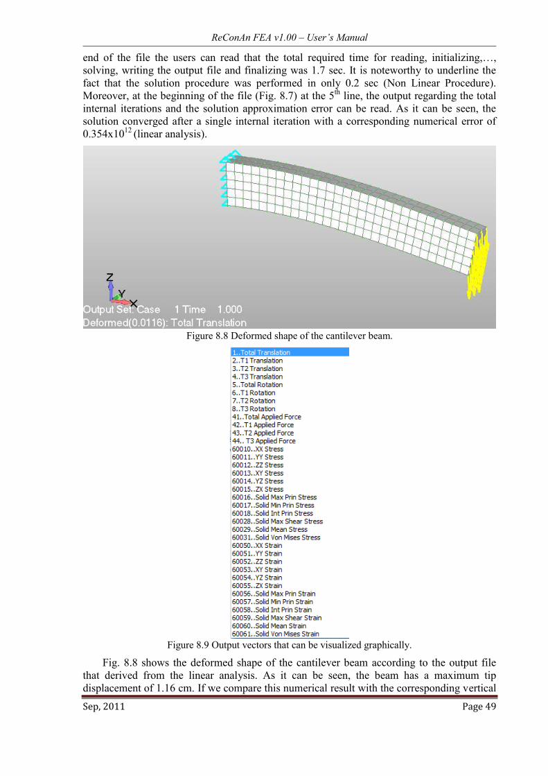
ReConAn FEA v1.00 – User’s Manual
Sep, 2011 Page 49
end of the file the users can read that the total required time for reading, initializing,…,
solving, writing the output file and finalizing was 1.7 sec. It is noteworthy to underline the
fact that the solution procedure was performed in only 0.2 sec (Non Linear Procedure).
Moreover, at the beginning of the file (Fig. 8.7) at the 5th
line, the output regarding the total
internal iterations and the solution approximation error can be read. As it can be seen, the
solution converged after a single internal iteration with a corresponding numerical error of
0.354x10¹²
(linear analysis).
Figure 8.8 Deformed shape of the cantilever beam.
Figure 8.9 Output vectors that can be visualized graphically.
Fig. 8.8 shows the deformed shape of the cantilever beam according to the output file
that derived from the linear analysis. As it can be seen, the beam has a maximum tip
displacement of 1.16 cm. If we compare this numerical result with the corresponding vertical

ReConAn FEA v1.00 – User’s Manual
Sep, 2011 Page 50
displacement that derived from the beam-element model of section 5.9 (1.15 cm), it can be
concluded that the hexahedral model results into a softer mechanical behavior due to its
numerical FE formulation. If a finer mesh is used the maximum computed tip displacement
would have increased even more, according to the mesh sensitivity phenomenon that
characterizes this type of discretizations.
When using the hexahedral element, the user is able to use several of the Femap’s
graphical illustration tools so as to visualize any resulted output. Fig. 8.9 shows the list of
choices that the user can select in order to graphically illustrate the resulted numerical output.
Fig. 8.10 shows the deformed shape and the von Mises stress contour of the cantilever
beam that resulted from the linear solution procedure. This graphical tool enables the user to
monitor and study the stress-strain distribution on the surface of any FE mesh. In addition to
that, the ability of viewing inside the mesh can be performed by executing the View
Advanced Post Dynamic Cutting command (Fig. 8.11).
Figure 8.10 Deformed shape and von Mises stress contour.
Figure 8.11 von Mises stress contour. Dynamic cut along the plane YZ.
8.1.2 Model with 20-noded Hexahedral Elements
In order to upgrade the hexahedral mesh of Fig. 8.1 from 8-noded to 20-noded, the user
has to execute the following command: Modify Update Elements Linear/Parabolic
Order (Fig. 8.12). The resulted hexahedral mesh can be depicted in Fig. 8.13 where it can be
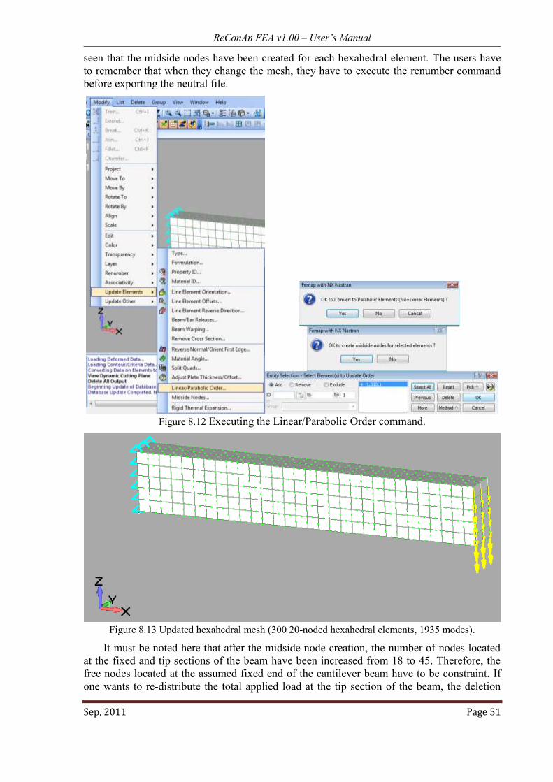
ReConAn FEA v1.00 – User’s Manual
Sep, 2011 Page 51
seen that the midside nodes have been created for each hexahedral element. The users have
to remember that when they change the mesh, they have to execute the renumber command
before exporting the neutral file.
Figure 8.12 Executing the Linear/Parabolic Order command.
Figure 8.13 Updated hexahedral mesh (300 20-noded hexahedral elements, 1935 modes).
It must be noted here that after the midside node creation, the number of nodes located
at the fixed and tip sections of the beam have been increased from 18 to 45. Therefore, the
free nodes located at the assumed fixed end of the cantilever beam have to be constraint. If
one wants to re-distribute the total applied load at the tip section of the beam, the deletion

ReConAn FEA v1.00 – User’s Manual
Sep, 2011 Page 52
and re-application of the concentrated load of 100 kN has to be performed. For our numerical
implementation, the load is re-distributed according to the above procedure and the nodes
that are located at the fixed end of the beam are constraint so as to achieve the same support
conditions with those applied for the case of the 8-noded hexahedral FE model.
After solving the linear solution problem the output file is imported in Femap and the
derived deformed shape is presented in Fig. 8.14. As it can be seen, the resulted maximum
displacement was 1.18cm, which confirms the softer numerical behavior of the 20-noded
quadratic isoparametric hexahedral element. The integration rule adopted for the case of the
20-noded hexahedral element is the 3x3x3 Gauss integration points and for the case of the 8-
noded hexahedral element is the 2x2x2 Gauss integration points.
Figure 8.14 Deformed shape of the cantilever beam. 20-noded hexahedral elements.
Figure 8.15 Time file for the case of the cantilever beam with 20-noded hexahedral elements.
Before moving to the presentation of nonlinear analysis with hexahedral elements, it
must be noted that stress-strain contouring is not available with 20-noded hexahedral
elements due to renumbering issues between Femap and ReConAn. Closing this section, the
computational performance is illustrated in Fig. 8.15 where the TIME.dat file is given.

ReConAn FEA v1.00 – User’s Manual
Sep, 2011 Page 53
8.2 Nonlinear Analysis with Hexahedral Elements
In this section, the nonlinear analysis of the previous cantilever beam will be presented.
Given the fact that the previous numerical implementation is already constructed (section
8.1.1), we are going to use its input file as a starting point while perform all the required
modifications so as to create the mesh of Fig. 8.16, define the nonlinear parameters of the
model’s material and readjust the solution algorithm’s parameters (Newton-Raphson).
8.2.1 Model with 8-noded Hexahedral Elements
As it can be seen in Fig. 8.16, it is assumed that the cantilever beam is connected to a
shear wall with a section 25x200 cm. This assumption is made so as to make the numerical
implementation more realistic and illustrate the nonlinear mechanical behavior of a full 3D
RC joint.
Figure 8.16 Hexahedral mesh of a RC cantilever beam supported on a shear wall.
After constructing the hexahedral mesh of Fig. 8.16, the next step is to set the nonlinear
material parameters to fc = 30 MPa and H = 0 GPa through the material edit tool (Figs. 8.17).
After defining the “Compression” limit stress, the “Nonlinear Type” is set to “Elasto-Plastic”
and the hardening parameter is set to 0 GPa (Fig. 8.17). The hardening parameter is set to 0
so as to illustrate the evolution of the plastification through the stress contour representation
after the nonlinear solution. As it was analyzed in section 6.1, the under study cantilever
beam section at the fixed end is completely plastified for a total load of 156.4 kN thus the
total applied load (100 kN) has to be increased. Therefore, the next step is to increase the
applied load to 200 kN by executing the command Modify Update Other Scale Load
command. After selecting all concentrated forces, the “Multiply by” factor is set to 2. This
ensures that all concentrated forces are multiplied by 1.6 and the total applied load should
result to 200 kN. This can be verified by performing the Sum Forces check through the Tools
Check menu.

ReConAn FEA v1.00 – User’s Manual
Sep, 2011 Page 54
After updating the forces array, the nonlinear parameters are updated through editing the
Nonlinear Analysis window. We select to apply the external force in 50 load increments and
the work convergence tolerance is set to 10-4
(Fig. 8.18). the final step, before exporting the
neutral file, is to check for any coincident nodes and renumber both nodes and elements by
executing the renumber command.
Figure 8.17 Editing of the material parameters.
Fig. 8.19 shows the initiation of yielding which occurs for a total applied load of 124 kN
and a corresponding tip displacement of 1.73 cm. This also complies with the numerical
findings of section 6.1, as it can be seen in the corresponding P-δ curve that derived when
using the NBCFB element (Fig. 6.5).
Fig. 8.20 shows the von Mises stress contour prior complete plastification of the fixed
end area of the cantilever beam. As it can be seen, the plastified area is approximately 1 m
thus the main nonlinearities are concentrated in the volume connected to the shear wall. It
must be noted that the 8-noded hexahedral element illustrates a stiffer behavior due to its
formulation. The 20-noded hexahedral element is the most suitable FE to analyze the
elastoplastic mechanical behavior of structures with homogenous materials (i.e. steel).

ReConAn FEA v1.00 – User’s Manual
Sep, 2011 Page 55
Figure 8.18 Editing the Nonlinear Analysis parameters.
Figure 8.19 Yielding initiation. Von Mises stress contour.
Figure 8.20 Von Mises stress contour prior complete plastification.

ReConAn FEA v1.00 – User’s Manual
Sep, 2011 Page 56
8.2.2 Model with 20-noded Hexahedral Elements
Fig. 8.21 shows the FE mesh of the 20-noded hexahedral elements after executing the
FE update command. The derived mesh is also updated (re-distribution of forces at the tip
section and fix the additional nodes at the support areas of the shear wall) and the neutral file
is created through the export neutral command. The FE mesh consists of 10,035 nodes, 1,700
elements and the total number of equations is 29,115. The total external load is 180 kN and it
is applied incrementally in 50 load steps.
Figure 8.21 20-noded hexahedral mesh.
Figure 8.22 P-δ curve. 20-noded hexahedral mesh.
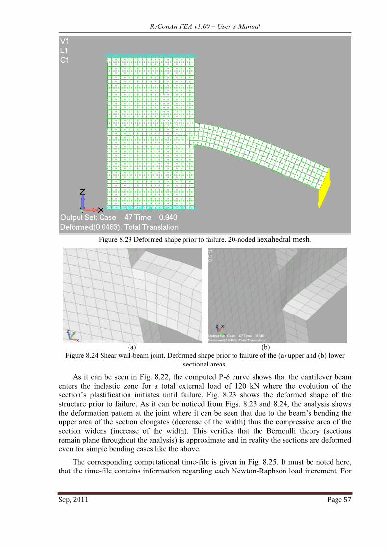
ReConAn FEA v1.00 – User’s Manual
Sep, 2011 Page 57
Figure 8.23 Deformed shape prior to failure. 20-noded hexahedral mesh.
(a) (b)
Figure 8.24 Shear wall-beam joint. Deformed shape prior to failure of the (a) upper and (b) lower
sectional areas.
As it can be seen in Fig. 8.22, the computed P-δ curve shows that the cantilever beam
enters the inelastic zone for a total external load of 120 kN where the evolution of the
section’s plastification initiates until failure. Fig. 8.23 shows the deformed shape of the
structure prior to failure. As it can be noticed from Figs. 8.23 and 8.24, the analysis shows
the deformation pattern at the joint where it can be seen that due to the beam’s bending the
upper area of the section elongates (decrease of the width) thus the compressive area of the
section widens (increase of the width). This verifies that the Bernoulli theory (sections
remain plane throughout the analysis) is approximate and in reality the sections are deformed
even for simple bending cases like the above.
The corresponding computational time-file is given in Fig. 8.25. It must be noted here,
that the time-file contains information regarding each Newton-Raphson load increment. For
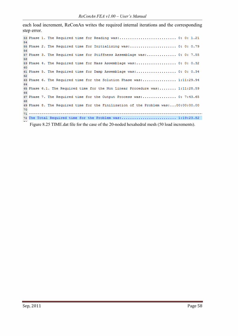
ReConAn FEA v1.00 – User’s Manual
Sep, 2011 Page 58
each load increment, ReConAn writes the required internal iterations and the corresponding
step error.
Figure 8.25 TIME.dat file for the case of the 20-noded hexahedral mesh (50 load increments).
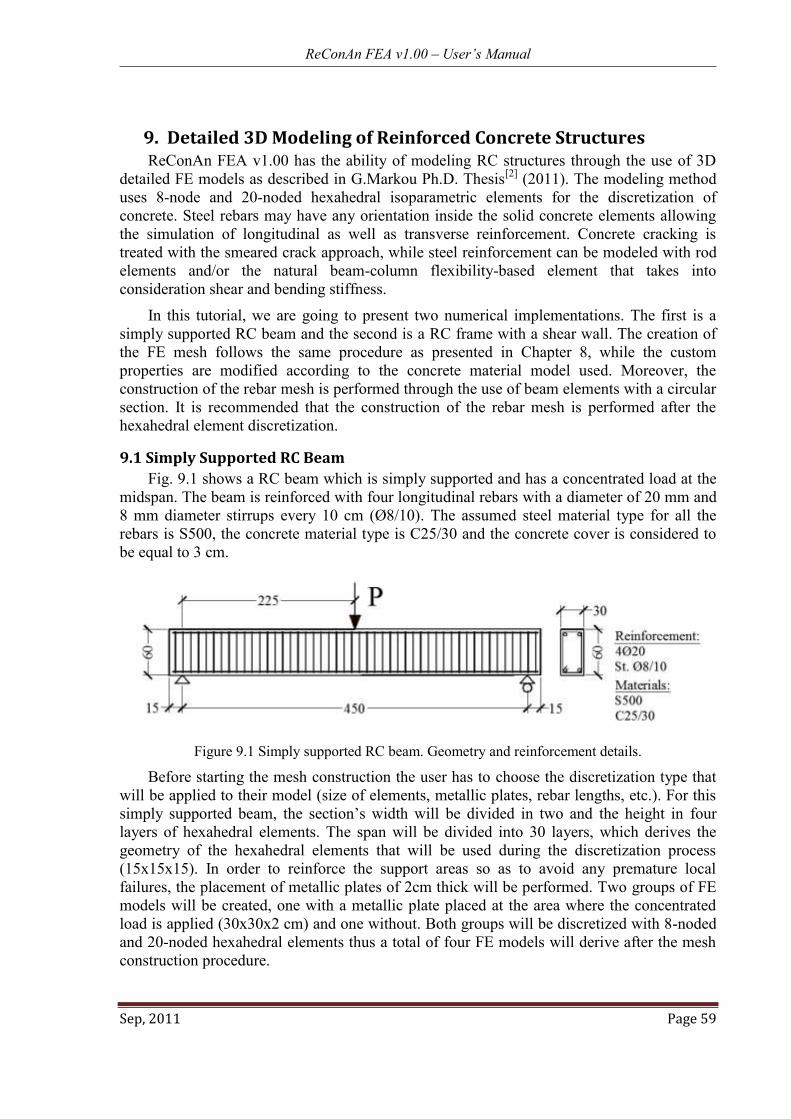
ReConAn FEA v1.00 – User’s Manual
Sep, 2011 Page 59
9. Detailed 3D Modeling of Reinforced Concrete Structures ReConAn FEA v1.00 has the ability of modeling RC structures through the use of 3D
detailed FE models as described in G.Markou Ph.D. Thesis[2]
(2011). The modeling method
uses 8-node and 20-noded hexahedral isoparametric elements for the discretization of
concrete. Steel rebars may have any orientation inside the solid concrete elements allowing
the simulation of longitudinal as well as transverse reinforcement. Concrete cracking is
treated with the smeared crack approach, while steel reinforcement can be modeled with rod
elements and/or the natural beam-column flexibility-based element that takes into
consideration shear and bending stiffness.
In this tutorial, we are going to present two numerical implementations. The first is a
simply supported RC beam and the second is a RC frame with a shear wall. The creation of
the FE mesh follows the same procedure as presented in Chapter 8, while the custom
properties are modified according to the concrete material model used. Moreover, the
construction of the rebar mesh is performed through the use of beam elements with a circular
section. It is recommended that the construction of the rebar mesh is performed after the
hexahedral element discretization.
9.1 Simply Supported RC Beam
Fig. 9.1 shows a RC beam which is simply supported and has a concentrated load at the
midspan. The beam is reinforced with four longitudinal rebars with a diameter of 20 mm and
8 mm diameter stirrups every 10 cm (Ø8/10). The assumed steel material type for all the
rebars is S500, the concrete material type is C25/30 and the concrete cover is considered to
be equal to 3 cm.
Figure 9.1 Simply supported RC beam. Geometry and reinforcement details.
Before starting the mesh construction the user has to choose the discretization type that
will be applied to their model (size of elements, metallic plates, rebar lengths, etc.). For this
simply supported beam, the section’s width will be divided in two and the height in four
layers of hexahedral elements. The span will be divided into 30 layers, which derives the
geometry of the hexahedral elements that will be used during the discretization process
(15x15x15). In order to reinforce the support areas so as to avoid any premature local
failures, the placement of metallic plates of 2cm thick will be performed. Two groups of FE
models will be created, one with a metallic plate placed at the area where the concentrated
load is applied (30x30x2 cm) and one without. Both groups will be discretized with 8-noded
and 20-noded hexahedral elements thus a total of four FE models will derive after the mesh
construction procedure.

ReConAn FEA v1.00 – User’s Manual
Sep, 2011 Page 60
9.1.1 Models with 8-noded Hexahedral and Rod Elements
For presentation reasons, only the first FE mesh will be analytically described during its
mesh development. The first step, when constructing the FE mesh, is to discretize the beam
into hexahedral elements. There are two different discretization methods that are available in
Femap. The first method is to create the geometry through lines, surfaces and volumes, while
assigning mesh attributes to the resulted geometric volumes so as to specify the element size
during the discretization procedure. The second method, which is recommended mostly for
cases where the mesh geometry is symmetric and repeats itself, the creation of nodes and
elements through the Model Node, Element and Mesh Copy Node, Element
commands.
When constructing a FE model which contains concrete hexahedral elements, a material
needs to be defined that will contain the concrete material characteristics and a steel material
for the rebars, respectively (if more than one concrete or steel materials are used then create
the required number of materials). In this numerical implementation the following
parameters will be used: fc = 25 MPa, νc = 0.2, Ec = 28 GPa, fy = 500 MPa, νs = 0.3, ES =
210 GPa and Ets = 2.1 GPa, where fc, ν, Ec, fy, ν, ES and Ets are the concrete’s cylindrical
uniaxial compressive strength, Poisson ratio, Young modulus, steel’s yielding stress, Poisson
ratio, Young modulus and hardening modulus, respectively. The concrete’s tensional
strength will be assumed to be equal to 5% of its uniaxial compressive strength. This
parameter is defined through the custom properties window. For the case of the concrete
material definition, the nonlinear parameters are not required since ReConAn incorporates all
the required data so as to proceed with the nonlinear analysis thus defining these four pre-
mentioned parameters and two additional that are related to the material type, is sufficient.
Figure 9.2 Define concrete material C25/30.
It is important to note at this point that the steel material for the case of the rebar
elements, is defined so as to be able to define the corresponding rebar element property. The
reinforcement material characteristics will be defined through the custom properties window
as it will be presented in this section. The steel material that was defined (Fig. 9.3) can be
also used by the steel hexahedral elements that will be positioned at the support and loading

ReConAn FEA v1.00 – User’s Manual
Sep, 2011 Page 61
areas of the beam for reinforcement reasons. It is strongly recommended that when users
define a material in Femap, regardless the fact whether materials are defined through the
custom properties window or not, they should always set the proper parameters. This will
help in avoiding errors when assigning the same material to multiple properties (in this case
the hexahedral property of the steel elements and the steel rebar elements).
Figure 9.3 Define steel material S500.
Figure 9.4 Mesh construction of the beam.
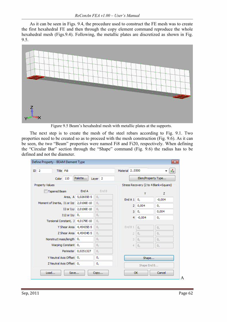
ReConAn FEA v1.00 – User’s Manual
Sep, 2011 Page 62
As it can be seen in Figs. 9.4, the procedure used to construct the FE mesh was to create
the first hexahedral FE and then through the copy element command reproduce the whole
hexahedral mesh (Figs.9.4). Following, the metallic plates are discretized as shown in Fig.
9.5.
Figure 9.5 Beam’s hexahedral mesh with metallic plates at the supports.
The next step is to create the mesh of the steel rebars according to Fig. 9.1. Two
properties need to be created so as to proceed with the mesh construction (Fig. 9.6). As it can
be seen, the two “Beam” properties were named Fi8 and Fi20, respectively. When defining
the “Circular Bar” section through the “Shape” command (Fig. 9.6) the radius has to be
defined and not the diameter.
A

ReConAn FEA v1.00 – User’s Manual
Sep, 2011 Page 63
B
C

ReConAn FEA v1.00 – User’s Manual
Sep, 2011 Page 64
D Figure 9.6 Rebar property definitions. A-B. Fi8 and C-D. Fi20.
Figure 9.7 Custom properties of Hexa8_C25 (concrete hexahedral elements).
The next step, before proceeding with the construction of the embedded rebar mesh, is to
customize the four properties related to the hexahedral and rebar elements. For the case of
the hexahedral element property, the parameters shown in Fig. 9.7 are defined. As it can be
seen in Fig. 9.7, the first parameter is set to 1 given that the numerical problem involves the

ReConAn FEA v1.00 – User’s Manual
Sep, 2011 Page 65
numerical modeling of a RC structural member. The second parameter is set to 3, which
defines the material used during the analysis (Modified Kotsovos & Pavlovic concrete
material model as it was proposed by Markou & Papadrakakis[2, 7]
). The remaining shear
factor β is set to 5% and the tensile strength to 5%. The “Elastic Limit” parameter refers to
the percentage on the concrete’s strength limit where the material is assumed to behave
elastically. When the stress exceeds this percentage the concrete material model is activated
accounting stiffness degradation according to the stress state of concrete thus for this
numerical implementation, the elastic limit is set equal to 50%, which is a recommended
value. The higher this value is the stiffer the numerical behavior of the concrete material
model. The geometric constraint parameter c refers to the mesh generation procedure[2, 8]
and
is set equal to 3. The parameter “Cracks/Internal Iteration” refers to the Kotsovos & Pavlovic
material model, which is this case does not apply and is set to 0. This parameter defines the
allowable crack openings per internal iteration.
Figure 9.8 Custom properties of Fi8 and Fi20 reinforced properties.
Fig. 9.8 shows the custom properties of the reinforcement property types which consist
of the following parameters:
1. "Slip Flag (0:NoSlip)"
2. "Type of Element for Reinf. 1:Rod 2:NBCFB(rect.) 3:NBCFB(circ.)"
3. "Number of Fibers (if NBCFB)"
4. "Number of Integ Points (if NBCFB)"
5. "Material Flag (1:Bilinear 2:Menegotto Pinto)"
6. "Flag (always 1.0)"
7. "Steel Young Modulus"
8. "Steel Poisson"
9. "Steel Hardening"
10. "Steel Fy"
11. "Steel Failure (ef = 0.12)"

ReConAn FEA v1.00 – User’s Manual
Sep, 2011 Page 66
12. "Reinforcement Flag (always 10)"
The first property parameter refers to the slip phenomenon, which in the current
ReConAn version is not taken into account, thus is set always to 0. The second parameter
provides the ability of selecting the element type that will be used for the simulation of the
reinforcement. There are three choices, the Rod element and the NBCFB element[2, 8]
with
rectangular and circular sections, respectively. As it can be seen (Fig. 9.8), the selected rebar
element type is Rod.
The third and fourth parameters refer to the case where the NBCFB element is used and
they refer to the number of fibers used to discretize the rebar section and the number of
Gauss-Lobato integration points, respectively. For the case where the circular section is used,
the default value of fibers is four. The fifth parameter sets the steel material model that is
going to be used during the nonlinear solution procedure. There are two steel material
models available, the bilinear and the Menegotto & Pinto[5]
material models. The selected
material model is the bilinear as it can be depicted in Fig. 9.8 (Flag = 1). The sixth parameter
has to be set always to 1.0.
Parameter 7-10, refer to the steel material characteristics and have to be defined by using
the same units system with that used when defining the geometrical and material
characteristics of the numerical model, which in this case is meters, kN and kPa. The values
that where defined are according to the material characteristics assumed in this numerical
implementation. The eleventh parameter also refers to a steel material characteristic which
denotes the steel’s failure strain ef. Finally, the last parameter is always set to 10 (rebar
element flag). It is noteworthy to point out at this point that the custom properties parameters
can be defined at any stage after the property definition procedure.
At this stage the model is ready to be enriched with embedded rebar elements. The
easiest way to create the embedded rebar mesh is to use the existing hexahedral nodes and
use the copy-node command so as to create the first elements.
As it can be seen in Fig. 9.9, the rebar mesh was constructed in such a way that each
initial rebar element penetrates two hexahedral elements. This is not a restraint since
parameter c can be set equal to 25 and use a single initial rebars so as to construct the
longitudinal rebar mesh. The user must have in mind that the post-processing of Femap will
use this mesh (Fig. 9.9) so as to represent graphically the numerical results thus when using a
single initial longitudinal rebar they will see a straight line that will not bend, even though
the embedded mesh generation procedure will be executed successfully. It is a graphical
hinge that can be overcome through the proper initial discretization.
The next step is to set the boundary conditions, support system and external loads. After
the definition of the appropriate constraint set, the left mid-nodes of the metallic plate are
constraint so as to behave as a 3D pin and the right mid-nodes of the support plate are
constraint so as to behave as a 3D roller (Fig. 9.10).
As Fig. 9.11 illustrates, the vertical mid-span load is distributed on the three nodes
located on the upper surface of the beam’s mid-section. The middle node is loaded with 240
kN and the two end nodes are loaded with 120 kN each (total applied load 480 kN). This
type of distribution will ensure that the phenomenon of node detachment due to local
cracking will be avoided. Following, the nonlinear analysis parameters are set, as illustrated
in Fig. 9.12. As it can be seen, the external load is applied incrementally and it is divided into
50 load increments. The corresponding work convergence tolerance is set to 10-4
. After
checking for coincident nodes and executing the renumbering command for both nodes and
elements, the neutral file is being exported and the analysis follows.

ReConAn FEA v1.00 – User’s Manual
Sep, 2011 Page 67
Figure 9.9 Construction process of the embedded rebar mesh.
Figure 9.10 Supports (Left) Pin and (Right) Roller.
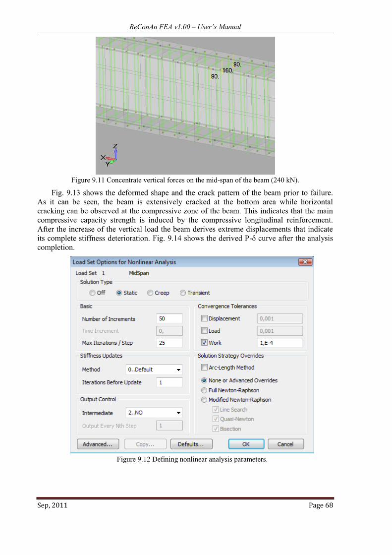
ReConAn FEA v1.00 – User’s Manual
Sep, 2011 Page 68
Figure 9.11 Concentrate vertical forces on the mid-span of the beam (240 kN).
Fig. 9.13 shows the deformed shape and the crack pattern of the beam prior to failure.
As it can be seen, the beam is extensively cracked at the bottom area while horizontal
cracking can be observed at the compressive zone of the beam. This indicates that the main
compressive capacity strength is induced by the compressive longitudinal reinforcement.
After the increase of the vertical load the beam derives extreme displacements that indicate
its complete stiffness deterioration. Fig. 9.14 shows the derived P-δ curve after the analysis
completion.
Figure 9.12 Defining nonlinear analysis parameters.

ReConAn FEA v1.00 – User’s Manual
Sep, 2011 Page 69
Figure 9.13 Deformed shape and crack pattern prior to failure (P = 336 kN).
Figure 9.14 P-δ curve of the simply supported beam. Steel hardening modulus equal to 2.1 GPa.
As it can be seen, the fact that the steel rebar elements were assumed to have a
hardening modulus equal to the 1% of the initial Young modulus, induced the required
plasticity in order for the beam to behave as high ductility structural member. If the
hardening modulus is set equal to zero for both longitudinal and stirrup reinforcement the
corresponding P-δ curve is that presented in Fig. 9.15. It is evident that the hardening
modulus plays a significant role during the nonlinear analysis, especially when yielding
occurs (P > 200 kN).
Figure 9.15 P-δ curve of the simply supported beam. Steel hardening modulus equal to zero.
After the completion of the nonlinear analysis and the output processing, ReConAn Eye
post-processing software initiates. This software was created in order to be able to illustrate
graphically the deformed shape of the FE mesh and the crack propagation according to the
nonlinear analysis. The graphical tools are all located in a pop-up window which appears
when the right button of the mouse is clicked on the screen (Fig. 9.16). When the user left

ReConAn FEA v1.00 – User’s Manual
Sep, 2011 Page 70
clicks on any command, then it is executed automatically as in any windows based software.
As it can be seen, the main commands relate to the ability of switching on/off nodes,
integration points, surface grid, solid surfaces, axis, rebar elements, etc. Moreover, there is
the ability of illustrating a specific deformed shape for a given load increment i. When the
corresponding command is executed (Draw Deformed Shape i) the program asks in the DOS
window from the user to enter the desired load step. After typing the load increment’s
number (Fig. 9.17) the enter key has to be pressed in order for the command to be executed.
In addition to that, the user can animate the deformed history of the numerical model and
visualize the crack pattern as it was computed from the FE analysis. The cracks can be
represented as circular or square planes. The command “Set Deformation Scale Factor” is
used to magnify the derived deformations and the “Set Time Step Duration (sec)” to define
the time interval between two load increments during the animation. The “Set Animation
Step” command is used so as to specify the number of load increments that will be skipped
during the animation. Meaning that if the user sets this value equal to 2, then the 1st, 3
rd,
5th
,… load increments will be used during the animation.
Figure 9.16 ReConAn Eye main command window.
All the commands that have the “>>>>>>>>” symbol in front of them refer to the
deformed state of the FE mesh and all the commands that have an asterisk “*” in front of
them refer to the embedded rebar elements. The View Modifier list contains information
regarding the use of the mouse, its wheel and keyboard arrows (zoom, pan, rotate, scale), and

ReConAn FEA v1.00 – User’s Manual
Sep, 2011 Page 71
some default view angles (XY, XZ, etc.). If the user wishes to illustrate the crack pattern
inside the beam, then by deactivating the solid surfaces the crack pattern presented in Fig.
9.18 will result.
Figure 9.17 ReConAn DOS window. Entering the load increment number.
Figure 9.18 Crack pattern inside the beam. Load increment 33.
Figure 9.19 FE mesh with metallic plates at support and loading areas.
In order to compare the computed results between the cases where a metallic plate is
used for the application of the external load the FE mesh in Fig. 9.19 is constructed. As it can
be seen, four prismatic elements (in red color) are attached at the compressive area of the
beam, while the external forces are deleted and re-defined so as to be assigned on the
corresponding nodes of the steel hexahedral elements. The hardening parameter of the steel
material is set to zero and the analysis is re-executed and derived curve is shows in Fig. 9.15,
which appears to behave slightly stiffer than the previous one. The compute crack pattern
prior to failure can be depicted in Fig. 9.20. Finally, the required computational time is given
in Fig. 9.21.

ReConAn FEA v1.00 – User’s Manual
Sep, 2011 Page 72
Figure 9.20 Crack pattern prior to failure. FE mesh with metallic plates at support and loading areas.
Figure 9.21 Required computational time for the nonlinear analysis of 18 load increments.
9.1.2 Models with 20-noded Hexahedral and Rod Elements
The last FE model that was presented in the previous section is used so as to update all
hexahedral elements into 20-noded isoparametric hexahedral elements through the
corresponding update command. The resulted FE mesh is given in Fig. 9.22 and after the
execution of the renumbering command, the exporting of the neutral file is performed.
Fig. 9.22 shows the crack pattern prior to failure as it was computed by the 20-noded
hexahedral FE mesh. The corresponding P-δ curve is compared with that resulted from the
analysis with 8-noded hexahedral elements and a metallic plate at the loading area. As it was
expected the updated mesh exhibits a softer behavior but manages to fail for a total vertical
load of 201.6 kN. This is attributed the FE formulation of the 20-noded hexahedral element
which uses 27 Gauss integration points. Fig. 9.24 shows the scaled deformed shape of the
embedded rebar elements as it was computed from the nonlinear analysis procedure.
Figure 9.22 Crack pattern prior to failure. 20-noded hexahedral FE mesh with metallic plates at
support and loading areas.

ReConAn FEA v1.00 – User’s Manual
Sep, 2011 Page 73
Figure 9.23 P-δ curve of 8-noded and 20-noded hexahedral elements. Simply supported beam with
steel hardening modulus equal to zero.
Figure 9.24 Deformed shape of the embedded rebar elements prior to failure. 20-noded hexahedral
FE mesh with metallic plates at support and loading areas.
9.1.3 Models with 8-noded Hexahedral and NBCFB Elements
It is very simple to update the current FE model with Rod embedded elements into a
model with NBCFB embedded elements. This is performed by double clicking on the rebar
property (Fi20), so as to activate it and its custom property through which the custom
properties are updated as shown in Fig. 9.25. The NBCFB embedded element with circular
section was selected and the number of fiber is set by default equal to 4 (Fig. 9.25). For this
numerical implementation the 8 mm rebar elements are modeled through the use of Rod
elements thus no custom properties update is performed. After updating the corresponding
property parameters the Apply button has to be pressed and the exporting procedure of the
neutral file has to be performed. The resulted P-δ curve is compared with the previous curves
in Fig. 9.26. It is important to note at this stage that the embedded NBCFB element can only
be combined with the 8-noded hexahedral element.

ReConAn FEA v1.00 – User’s Manual
Sep, 2011 Page 74
Figure 9.25 Custom properties of Fi20 with NBCFB embedded element attributes.
Figure 9.26 Comparison of P-δ curves of the simply supported beam. Steel hardening modulus equal
to zero.

ReConAn FEA v1.00 – User’s Manual
Sep, 2011 Page 75
9.2 RC Frame with Shear Wall
The second numerical implementation involves the nonlinear analysis of a RC frame with a
shear wall. Fig. 9.27 shows the geometrical features of the frame, which has a net span of 5
m and it consists of a shear wall (200x25 cm), a beam (25x50 cm) and a column (50x25 cm).
The frame has a total height of 3.5 m and its reinforcement details are given in Fig. 9.27. The
material properties considered for this numerical test are given in Table 9.1. Two types of
external loads are being applied: a) A vertical static linear concentrated load placed at the top
of the shear wall and column, respectively; b) a horizontal static nonlinear load on the upper
left region of the frame (Fig. 6.27).
The vertical loads V1 and V2 were assumed to be equal to the 20% of the axial capacity of
each structural member (SW and C in Fig. 9.27). These two vertical loads and the loads that
derive from the self-weight of the structure are applied entirely at the first load step. The
horizontal load H1 is divided into 40 load steps and it is applied incrementally until failure.
The work convergence tolerance, for the nonlinear analysis procedure, was set to 10-4
. It is
very important to state here that during the internal iterative procedure, the Newton-Raphson
algorithm checks if convergence is achieved at the end of each internal iteration, while if
after the 10th
iteration the solution has not yet converged, the algorithm automatically
increases the convergence tolerance by 10 (if initial tolerance 10-4
the increased tolerance
becomes 10-3
) so as to achieve convergence. This is applied only for the internal iterations
that exceed the 10th
internal iteration without achieving convergence. The user can monitor
the each internal iteration error through the DOS window of ReConAn and the TIME.dat file
which writes the final error for each load increment (Fig. 9.34).
Figure 9.27 RC frame. Geometric features and reinforcement details.
The FE mesh is shown in Figs. 9.28 and 9.29 where it can be observed that the 8-noded
hexahedral FE is used for discretizing the concrete domain and the longitudinal embedded
rebar elements are constructed so as to penetrate two hexahedral elements and the rest of the
reinforcement one initial rebar element was used. The total number of hexahedral elements is

ReConAn FEA v1.00 – User’s Manual
Sep, 2011 Page 76
576 and the total number of the embedded rebar elements is 6,608. The footings are also
modeled and their lower and side nodes are fixed (Fig. 9.28).
Material
Young
Modulus
(GPa)
Hardening
Modulus
(GPa)
Yielding
Stress
(MPa)
Compressive
Strength
(MPa)
Poisson
Ratio
Concrete 28 - - 30 0,17
Steel 190 1,9 500 - 0,3 Table 9.1 RC frame. Material details.
Figure 9.28 RC frame with shear wall. 8-noded hexahedral discretization.
Figure 9.29 RC frame with shear wall. Initial embedded rebar elements.
Seven properties are required (two solid and five beam) so as to construct the FE mesh:
1. Solid concrete property (8-noded hexahedral elements).
2. Solid steel property (8-noded hexahedral elements for the metallic plates).
3. Beam properties for the reinforcement with diameter:
I. Ø8
II. Ø12
III. Ø16

ReConAn FEA v1.00 – User’s Manual
Sep, 2011 Page 77
IV. Ø18
V. Ø22
For this numerical implementation the rebar elements with diameter of 22 mm are
modeled with NBCFB (Fig. 9.30) and the rest are modeled with the Rod element. It is very
important to organize the FE mesh especially when dealing with structures that have many
structural members thus large number of finite elements. This can be implemented through
the use of layouts, that Femap provides as an organization tool during pre- and post-
processing.
Figure 9.30 Custom properties of Fi22 with NBCFB embedded element attributes.
Figure 9.31 RC frame with shear wall. P-δ curve.

ReConAn FEA v1.00 – User’s Manual
Sep, 2011 Page 78
After the solution has completed, the derived P-δ curve is shown in Fig. 9.31, while the
computed crack pattern prior to failure can be seen in Fig. 9.32. Moreover, the von Mises
strain contour prior to failure is given in Fig. 9.33 through which the analyst can allocate the
areas of strain concentration.
A.
B. Figure 9.32 Crack pattern and deformed shape prior to failure A. XZ view and B. 3D view
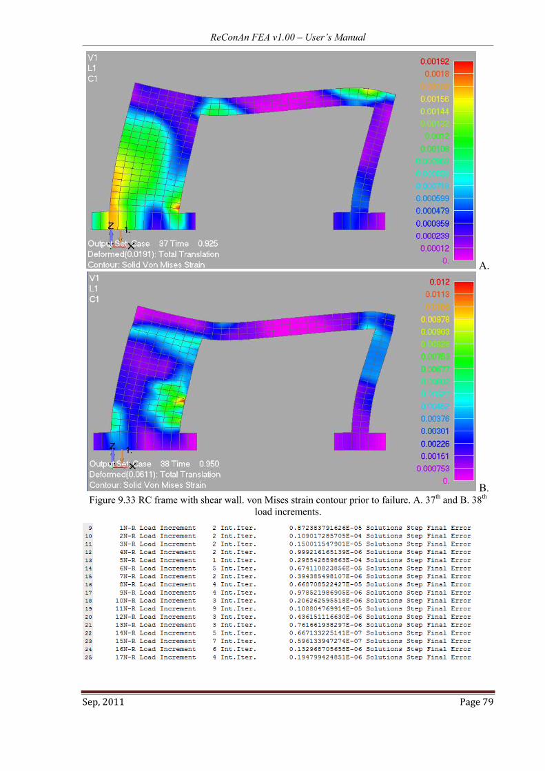
ReConAn FEA v1.00 – User’s Manual
Sep, 2011 Page 79
A.
B. Figure 9.33 RC frame with shear wall. von Mises strain contour prior to failure. A. 37
th and B. 38
th
load increments.

ReConAn FEA v1.00 – User’s Manual
Sep, 2011 Page 80
Figure 9.34 RC frame with shear wall. Numerical error and required internal iterations per each load
increment.
As it was said previously, Fig. 9.34 shows the required internal iterations per Newton-
Raphson load increment, the final load increment’s numerical error and the required
computational time. In addition to that, in lines 47 and 48 (Fig. 34) there are two warning
messages that inform the user that failure of rebar element 1 in hexahedral elements 2504
and 2505 occurred in Newton-Raphson load increment 39. The hexahedral elements’ ID are
those used in Femap but the corresponding rebar elements’ ID are referring to the local
numbering system of embedded rebar elements used in ReConAn. Finally, as it can be seen
in Fig. 9.34, the solution of 39 nonlinear steps required 1 min and 57 sec.

ReConAn FEA v1.00 – User’s Manual
Sep, 2011 Page 81
10. Hybrid Modeling (HYMOD) One of the main reasons for using the HYMOD is to reduce significantly the number of
degrees of freedom (dof) in order to be able to simulate full-scale structures with the required
accuracy at an affordable computational time. In the case of RC structures, the FE model
reduction (Fig. 10.1) requires the determination, by the user, of the length Li so that the
derived model will meet the objectives stated previously[2, 9]
. According to the parametric
investigation presented in [2], the recommended length Li can be set between H-2H, where H
is the section’s height.
Figure 10.1 Discretization of joints with detailed solid and beam elements. Reinforcement details and
fiber discretization of the beam-column sections[2]
.
Figure 10.2 RC Frame. Discretization schemes with different levels of model reduction
[2].

ReConAn FEA v1.00 – User’s Manual
Sep, 2011 Page 82
Reduction Level
of the Model Description
0 The whole structure is discretized with 3D solid elements
1
Shear dominated structural members (shear walls, junctions etc.) are
discretized with solid elements and the remaining parts of the structure with
beam elements.
2 Shear walls are discretized with solid elements and the rest of the structure
with beam elements.
3 The whole structure is discretized with beam elements. Table 10.1 Discretization with beam and solid elements. Description of the Reduction Levels
[2].
In this Chapter, two numerical implementations are going to be presented, a steel
cantilever beam and a RC frame. As it was presented in Markou & Papadrakakis[9]
(2011)
research work, when constructing a Hybrid FE mesh the user has to select the level of
reduction (Reduction Level “RL”) so as to reduce the solid FE mesh (Fig. 10.2 and Table
10.1), which is named as the RL0 case (no reduction is applied). This FE mesh description
will help the simplification on naming the derived FE meshes after the reduction of the initial
unreduced FE solid mesh.
10.1 Cantilever Steel Beam
The proposed HYMOD combines hexahedral and beam finite elements where the
coupling between them is achieved with kinematic constraints[2, 9]
. The structural members
that are shear dominated, such as shear walls and joints are discretized with 8-node or 20-
noded hexahedral elements while the rest of the structure is discretized with beam RC or/and
steel elements.
So as to illustrate the FE model construction process, the cantilever beam of section 8.1
is going to be analyzed through the use of two different Hybrid FE meshes. Both FE meshes
will assume a length Li = 1 m, which will be discretize with hexahedral elements (8-noded
and 20-noded hexahedral elements) while the rest of the beam is discretized with a single
NBCFB element (Fig. 10.3).
A. B.
Figure 10.3 Cantilever beam. Hybrid FE mesh with A. 8-noded and B. 20-noded hexahedral elements.
To construct the Hybrid FE mesh, the hexahedral discretization is performed as shown
in Fig. 10.4a. Following, the nodes of the beam type element are created (Fig. 10.4b), which
are positioned on the longitudinal axis of the cantilever beam’s geometry. An easy way to
perform the beam element’s nodes construction is to copy the middle lower node of the
interface section by using the Global Axis method 25cm along the positive direction of the z
global axis. The next step is to create the beam FE through the Model Element command
and the model in Fig. 10.4c will derives.

ReConAn FEA v1.00 – User’s Manual
Sep, 2011 Page 83
As it was described in [2, 9], several researchers proposed techniques in order to achieve
mesh coupling of different type of elements. In ReConAn FEA the coupling between the two
types of elements is treated as a kinematic constraint which considers that each hexahedral
node, located at the interface between the beam and the solid elements, will displace
according to standard kinematic relationships. In order for ReConAn FEA to acquirer the
proper data regarding the nodes located on the interface, where hexahedral nodes are
controlled by the master node of the beam, a rigid element has to be created so as to specify
the master node and the slave hexahedral nodes. This is performed through the execution of
the Model Element command, while selecting the Rigid type element (Fig. 10.5). After
defining the master node and slave nodes located on the interface, the final model derives as
shown in Fig. 10.4d. The rigid element does not require the definition of a property. It is
highly recommended to use the View Options window (f6 shortcut key) so as to extrude the
cross section of the beam type element in order to assure graphically that the section of the
beam matches the geometry of the hexahedral elements (Fig. 10.3). Finally, when
performing the check for coincident nodes the master beam node must never be merged with
a corresponding hexahedral node even in the case where these two nodes coincide.
A
B
C

ReConAn FEA v1.00 – User’s Manual
Sep, 2011 Page 84
D Figure 10.4 Cantilever beam. Hybrid FE mesh construction procedure.
Figure 10.5 Rigid element definition.
A

ReConAn FEA v1.00 – User’s Manual
Sep, 2011 Page 85
B Figure 10.6 Cantilever beam. Deformed shapes of the A. 8-noded and B. 20-noded Hybrid FE models.
After solving the linear static problem the output file is imported and the computed
deformed shapes are given in Fig. 10.6 for both models. As it can be seen the derived
displacements are 1.14 and 1.15 cm for the 8-noded and 20-noded Hybrid models,
respectively. As it was expected the behavior of the Hybrid models is slightly stiffer than
those of the unreduced model.
10.2 RC Frame
Fig. 10.7 shows the four FE models constructed for the purpose of this numerical
implementation representation. The RC frame of section 9.2 is used so as to apply the three
reduction levels as they are proposed in [2, 9]. The material characteristics used in this
numerical implementation are those depicted in Table 9.1. The hexahedral elements use to
discretize in detail the concrete volume was the 8-noded element and the embedded rebar
elements were modeled with Rod and NBCFB elements (see section 9.1). It must be noted
that the Rigid Elements shown in Fig. 10.6 are modeled with steel beam type elements with
large Young modulus values. This is performed so as to account for the joints’ offset.
Figure 10.7 RC frame. FE meshes.

ReConAn FEA v1.00 – User’s Manual
Sep, 2011 Page 86
The nonlinear solution procedure assumes that the horizontal force is applied
incrementally in 25 load steps and the convergence tolerance is set to 10-4
(work). The
derived P-δ curves are shown in Fig. 10.8.
Figure 10.8 RC frame. P-δ curves.
ReConAn FEA v1.00 – User’s Manual
Sep, 2011 Page 87
References
[1] Siemens PLM Software (2009), “World-class finite element analysis (FEA) solution for the
Windows desktop”, Siemens Product Lifecycle Management Software Inc.
[2] Markou G. (2011), “Detailed Three-Dimensional Nonlinear Hybrid Simulation for the
Analysis of Full-Scale Reinforced Concrete Structures”, Ph.D. Thesis, Institute of Structural
Analysis and Seismic Research, National Technical University of Athens.
[3] EN1998, Eurocode 8, “Design of structures for earthquake resistance”.
[4] Kent D.C. and Park R. (1971), “Flexural Members with Confined Concrete”, Journal of the
Structural Division, ASCE, Vol. 97(ST7).
[5] Menegotto M. and Pinto P.E. (1973), “Method of Analysis for Cyclically Loaded Reinforced
Concrete Plane Frames Including Changes in Geometry and Non-Elastic Behavior of Elements
under Combined Normal Force and Bending”, Proceedings, IABSE Symposium on Resistance
and Ultimate Deformability of Structures Acted on by Well Defined Repeated Loads, Lisbon,
pp.15-22.
[6] Kotsovos M.D. and Pavlovic M.N. (1995), “Structural Concrete – Finite-element analysis for
limit-state design”, Thomas Telford Publications.
[7] Markou G. and Papadrakakis M. (2010), “Detailed Three-Dimensional Modeling of
Reinforced Concrete Structures”, 9th HSTAM International Congress on Mechanics, Limassol,
Cyprus, 12-14 July.
[8] Markou G. and Papadrakakis M. (2010), “Generating Embedded Reinforcement in Hexahedral
Elements for Concrete Simulation”, 9th HSTAM International Congress on Mechanics,
Limassol, Cyprus, 12-14 July.
[9] G. Markou and M. Papadrakakis, “Non-Linear Simulation of Real-Scale RC Structures with
Detailed and Hybrid Finite Element Models”, 7th GRACM International Congress on
Computational Mechanics Athens, 30 June – 2 July 2011.