Reconciling High Food Prices with Engel and Prebisch-Singer

John Baffes jbaffes@worldbank.org

Xiaoli L. Etienne

xliao3@illinois.edu

February 21, 2014

ABSTRACT: During the past decade, food prices experienced the longest and broadest boom since World

War II. Income growth in emerging economies has been often cited as a key driver of the boom. Indeed,

low and middle income countries grew at 6.4 percent per annum during 2004-13, the highest of any 10-

year period since 1960—China and India grew nearly 10 percent during this period. Based on a reduced

form price determination model and annual data since 1960, this paper shows that income has a negative

and highly significant effect on real food commodity prices. This finding is consistent with and Engel’s

Law and Kindleberger’s thesis, the predecessor of the Prebisch-Singer hypothesis. Moreover, it is shown

that income’s negative impact on real prices operates through the manufacture price channel (the defla-

tor), thus weakening the view that income growth exerted upward pressure on food prices. Other key

drivers include (in order of importance) the role of energy costs, physical stocks, and monetary conditions. 

 

JEL CLASSIFICATTION: E31, O13, Q02, Q11, Q18 

 

KEY WORDS: Food prices, commodity price boom, Prebisch-Singer hypothesis, Engel’s Law

This paper was presented at the International Conference on Food Price Volatility: Causes and

Consequences, held in Rabat, Morocco (February 25-26, 2014). The conference was co-sponsored

by the Research Department of the International Monetary Fund, the OCP Policy Center, and

the Center for Technology and Economic Development of New York University. We would like

to thank Ataman Aksoy for comments on an earlier draft.

— 1 —

1. Introduction

During the past decade, commodity prices experienced the longest and broadest post-

World War II boom. Indeed, after declining for nearly three decades, world prices of

food commodities doubled in less than a decade. The boom took place at a time when

emerging economies experienced unprecedented growth as well. Low and middle in-

come countries grew at an annual average of 6.4 percent during 2004-13, the highest of

any 10-year period since 1960. China and India, two countries that account for more

than one third of world’s population, grew nearly 10 percent per annum during this pe-

riod.

Income growth in emerging economies has been often cited as a key driver of

past decade’s food price increases. Krugman (2008), for example, argued that the up-

ward pressure on grain prices is due to the growing number of people in emerging

economies, especially China, who are becoming wealthy enough to emulate Western

diets. Likewise, Wolf (2008) concluded that strong income growth by China, India, and

other emerging economies, which boosted demand for food commodities, was the key

factor behind the post-2007 increases in food prices. Similarly, the June 2009 issue of Na-

tional Geographic noted that demand for grains has increased because people in coun-

tries like China and India have prospered and moved up the food ladder. Other authors

have mentioned income growth as well (see, for example, Roberts and Schlenker 2013

and Hochman et al. 2011).

The above views reflect a widely held belief that income-driven demand growth

leads to price increases in food commodities, especially during the recent boom. How-

ever, historically the views on the relationship between income growth, food consump-

tion, and food prices were not so uniform. More than one and a half century ago, Engel

(1857) observed that poor families spend a greater proportion of their total expenditure

on food, thus leading to the so-called Engel’s Law of less than unitary income elasticity

of food commodities. Several decades later, Kindleberger (1943, p. 349) argued that

“[t]he terms of trade [ToT] move against agricultural and raw material countries as the

world’s standard of living increases (except in time of war) and as Engel’s Law of con-

sumption operates. The elasticity of demand for wheat, cotton, sugar, coffee, and bana-

nas is low with respect to income.” Because the income-food price relationship is

bounded by Engel’s Law and likely declines in ToT, any conclusion on its validity or

strength should be based on empirical verification.

Kindleberger’s thesis was empirically verified by Prebisch (1950) and Singer

(1950) as well as by Kindleberger (1958) himself. By many accounts, the declining ToT

views along with empirical verification (later coined as the Prebisch-Singer hypothesis)

formed the intellectual foundation on which the industrialization policies of the 1960s

and 1970s were based upon, that is heavy taxation of primary commodity sectors in fa-

— 2 —

vor of manufacture products, especially in low income countries.

This paper shows that income has a negative and highly significant effect on ToT

for food commodities, a result which is consistent with the Prebisch-Singer hypothesis.

The paper also shows that income’s impact on ToT operates mainly through the manu-

facture price channel. These results weaken the view that income growth by emerging

economies has played a key role during the past decade’s run up of food prices. The re-

sults are also consistent with the lower bound of Engel’s Law. Other key findings in-

clude the importance of energy costs, physical stocks, and (less so) monetary conditions.

The rest of the paper proceeds as follows. The next section discusses the views on

the relationship between income and commodity prices, beginning with Engel’s Law,

Kindleberger’s thesis, and Prebisch-Singer hypothesis; it also reviews the literature of

the latter. Section 3 introduces a model testing the Prebisch-Singer hypothesis by con-

trolling for the key sectoral and macroeconomic fundamentals affecting food prices.

Section 4 discusses the results on the Prebisch-Singer hypothesis and Engel’s Law, it

checks robustness with respect to various measures of income, and also discusses the

role of the remaining fundamentals. The last section concludes and discusses policy rel-

evant issues.

2. From Engel to Kindleberger and Prebisch-Singer

Based on expenditures of 153 Belgian families in 1853, Engel (1857) noted that "[t]he

poorer a family, the greater the proportion of its total expenditure that must be devoted

to the provision of food” and later concluded that “… the wealthier a nation, the smaller

the proportion of food to total expenditure.” (Quoted in Stigler 1954, p. 98). Following

Engel’s observation, at least three competing views attempted to explain and forecast

the long term behavior of the terms-of-trade faced by developing countries (Rostow

1950, Kindleberger 1958). First, a supply-side view predicted that primary commodity

prices will increase faster than manufacture prices due to resource constraints of the

former and technological improvements of the later—to a certain extent, this view was

consistent with a Malthusian path. A second view assumed that ToT will follow in-

vestment cycles. Investment expansion will induce supply response in manufacture

goods, leading to lower prices, thus increasing the ToT. Conversely, investment contrac-

tion would lead to declining ToT. Proponents of a third view argued that ToT will fol-

low a downward path because income growth leads to smaller demand increases in

primary commodities than manufacture products, an outcome which is consistent with

Engel’s Law.

While no dominant view emerged until the Second World War, the negative in-

come-ToT relationship became the prevailing position after the War. A turning point

was Kindleberger’s (1943) argument that “[i]f the agricultural and raw material coun-

tries of the world want to share the increase in the world’s productivity, including that

— 3 —

in their own products, they must join in the transfer of resources from agriculture, pas-

toral pursuits, and mining to industry.” Other authors, however, warned against such

policies. For example, Johnson (1947) argued that the agricultural sector required few

interventions. Friedman (1954) disputed the benefits of managing commodity income

variability. Johnson and Mellor (1961) severely criticized the pro-urban policies preva-

lent in many developing countries. Despite such warnings, Kindleberger’s views domi-

nated the post-war policy agenda and set the stage for the post-war industrialization

policies in developing countries.1

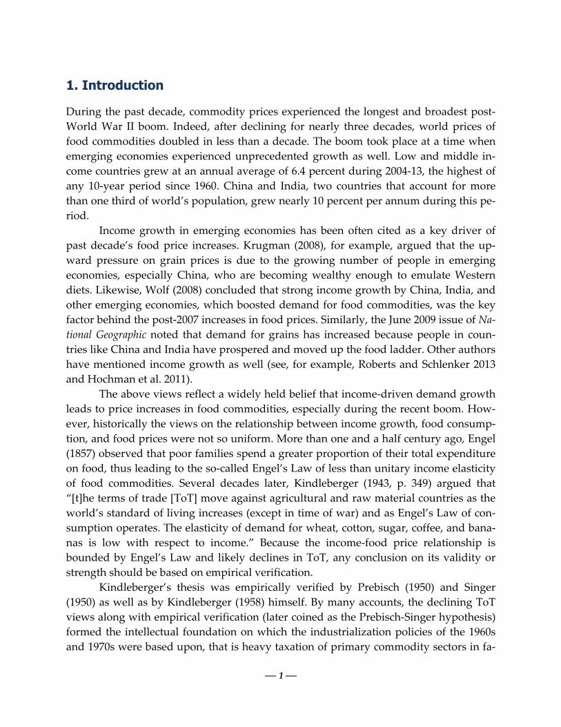
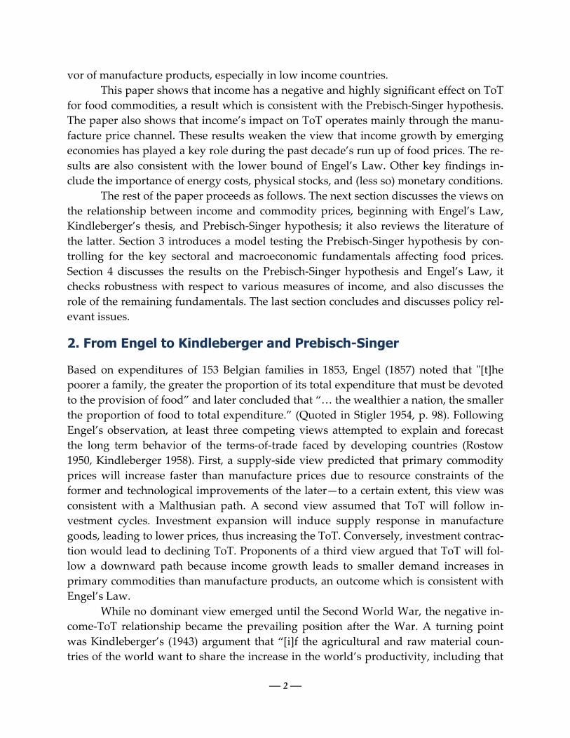
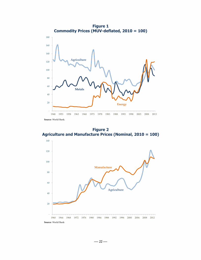
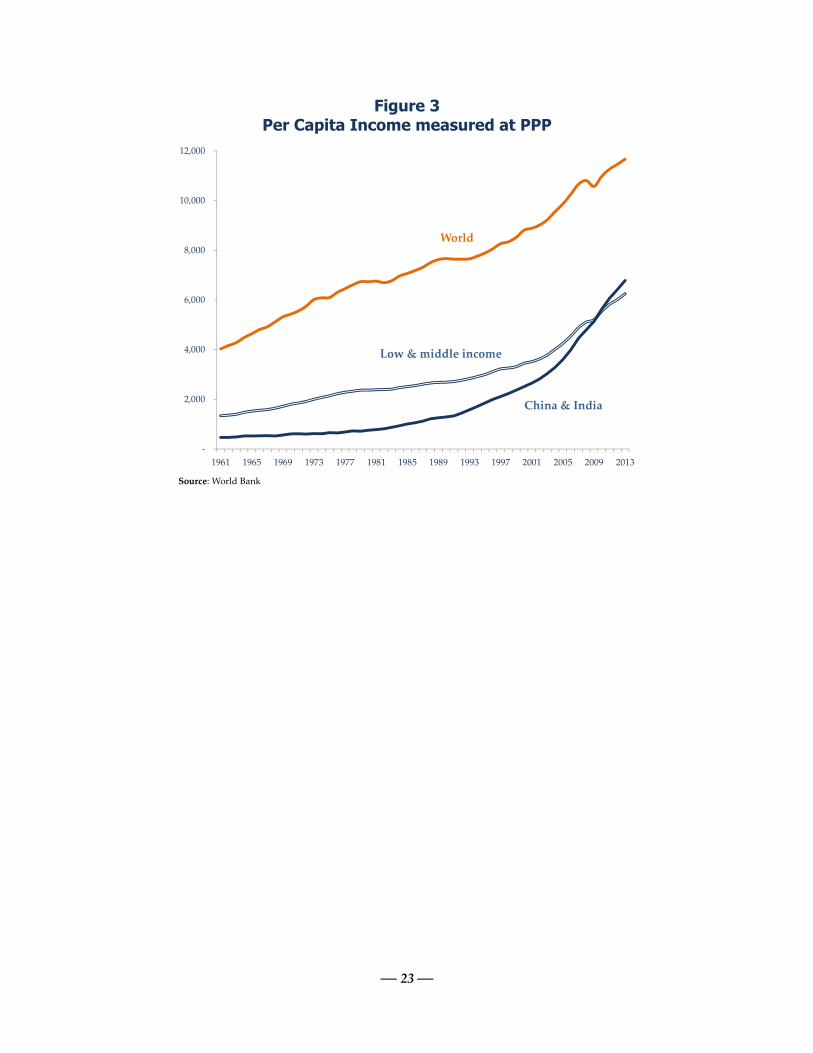
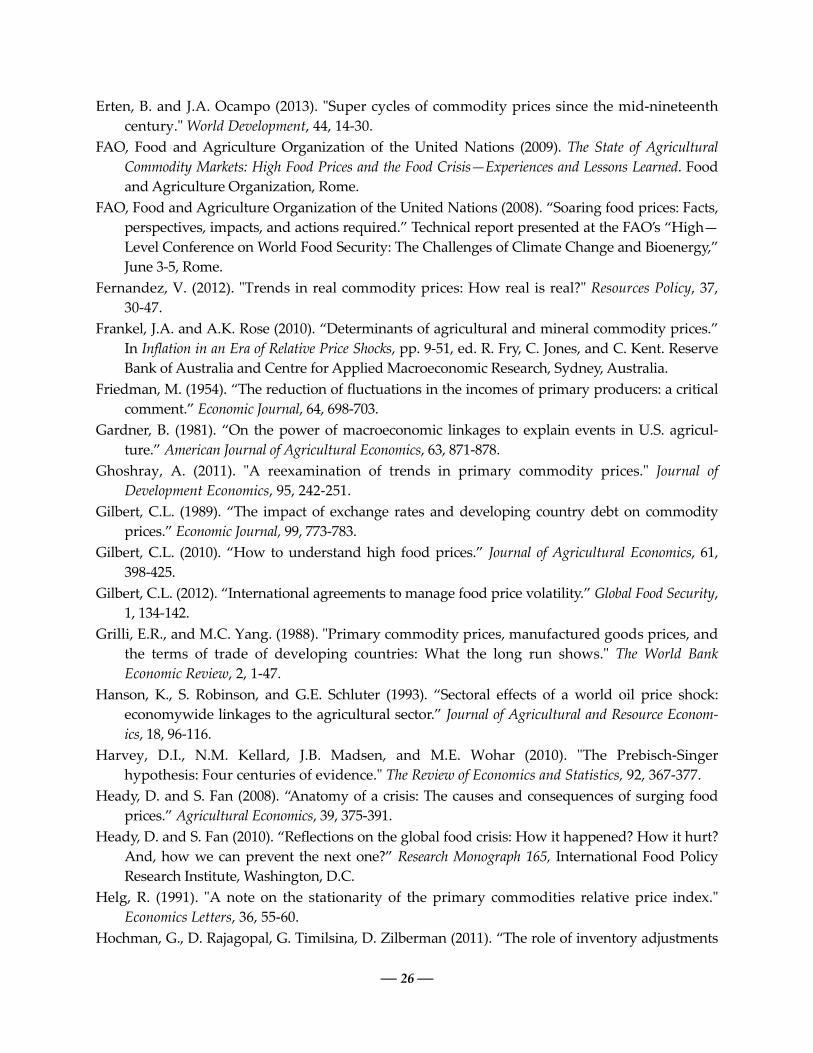
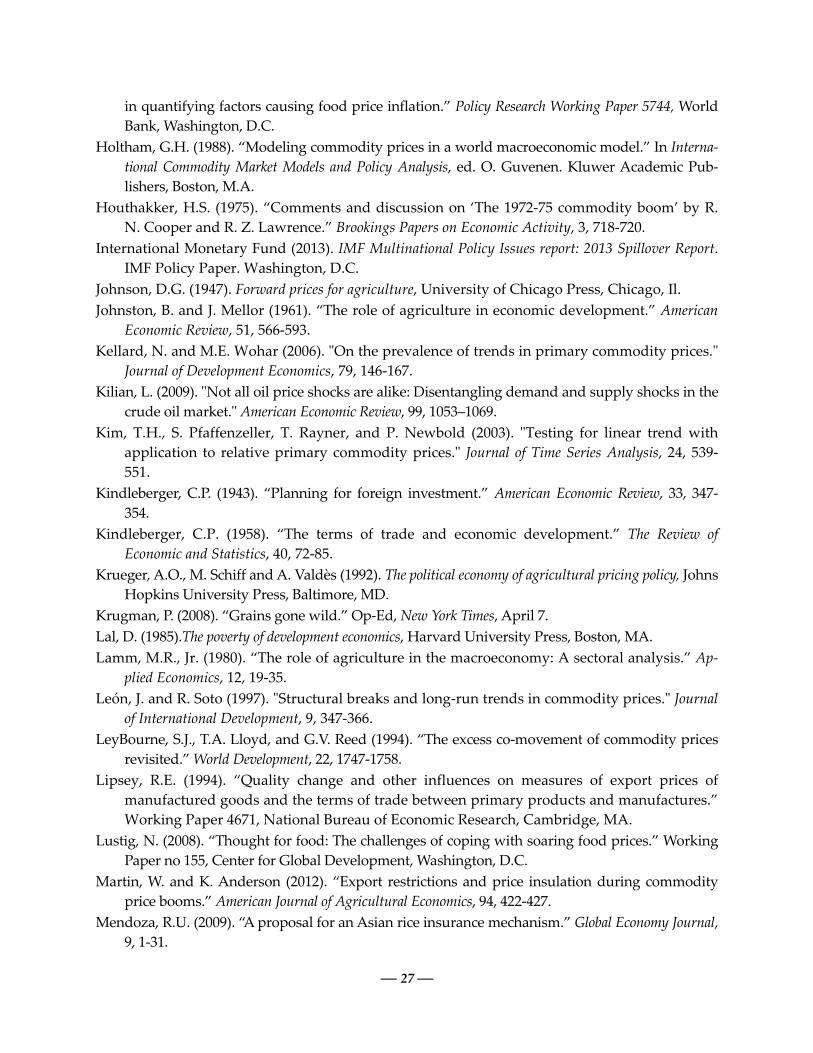
The long term behavior of ToT received renewed attention, beginning in the late

1980s. At least three reasons account for such attention. First, after the boom of the early

1970s, most commodity prices experienced large declines, subsequently stabilizing at

much lower levels (see figure 1 for the ToT of the three key indices and figure 2 for the

nominal agriculture and manufacture indices). Therefore, the Prebisch-Singer hypothe-

sis began fitting the data well. These declines are in sharp contrast to the increases dur-

ing the two decades following the war where food prices spiked on fears of a prolonged

conflict in the Korean peninsula (Korean War) while metal prices experienced sustained

boom because of Europe’s reconstruction and Japanese expansion. Second, numerous

authors began questioning the bias against primary commodity sectors. For example,

Bauer (1976) and Lal (1985) severely criticized pricing policies and marketing arrange-

ments in commodity-dependent developing countries. Bates (1981) argued that in order

for rural communities to prosper, most developing government policies concerning

markets would need to change. The tide turned against industrialization policies fol-

lowing the publication of two World Bank reports: The 1985 World Development Report

(World Bank 1995), which focused on the problems associated with policy interventions

in agricultural commodity markets, and the detailed assessment of distortions affecting

primary commodity sectors of developing countries by Krueger, Schiff and Valdès

(1992). Third, research on long term behavior of ToT was further aided by two influen-

tial papers. On the econometric side, Engle and Granger (1987) introduced improved

testing procedures that enabled researchers to distinguish between meaningful long

term relationships and spurious correlations. On the data side, Grilli and Yang (1988)

compiled a data base of 24 internationally-traded primary commodity prices since 1900

that was utilized (and updated) by numerous authors.

More than 30 papers published in academic journals have examined the

1 Kindleberger’s influence on world economic affairs should not be surprising. In addition to being a lead-

ing architect of the Marshall Plan, he voiced an early opinion on the nature of post-war development

lending operations: “If time permitted, it might be stimulating to analyze a number of knotty aspects of

an international development loan operation: how would productivity be defined in order to qualify for a

loan from the international development authority or whatever institution was created to perform that function?”

(Kindleberger 1943, p. 353, emphasis added). The Bretton Woods institutions (International Monetary

Fund and the World Bank) became operational two years later.

— 4 —

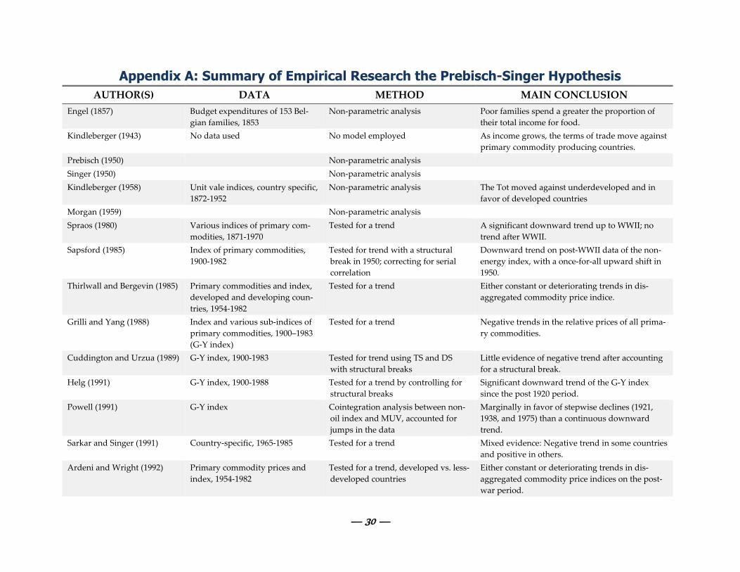
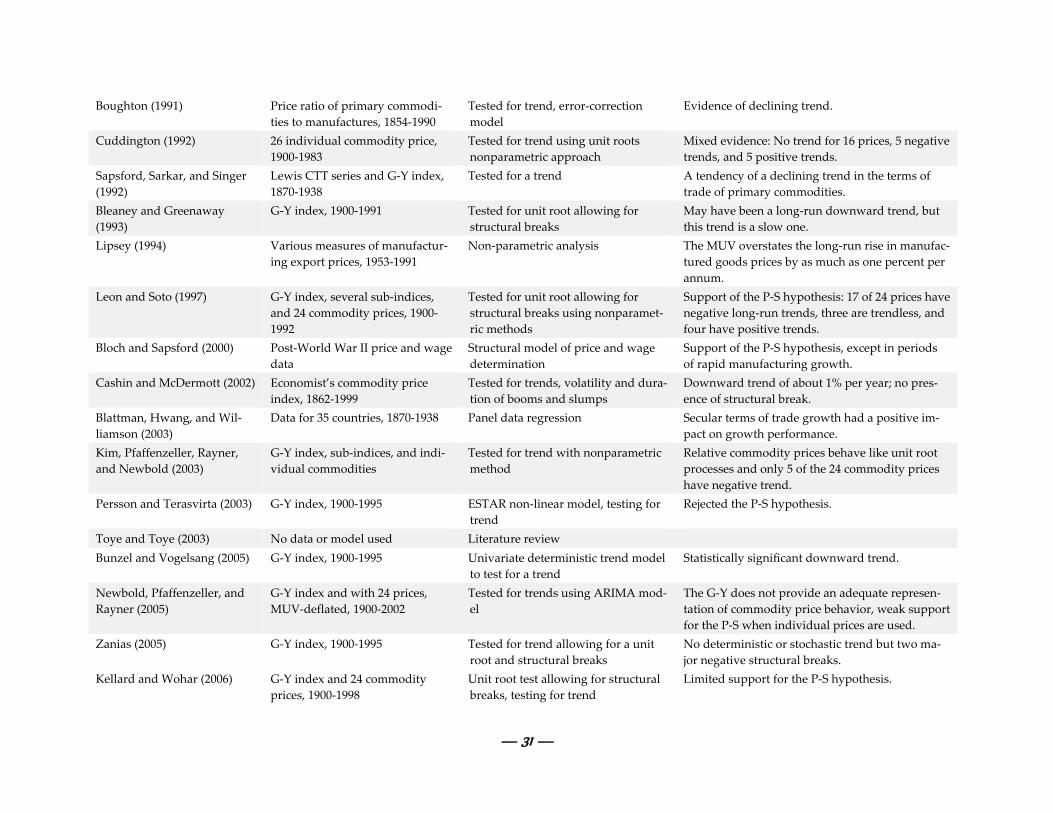
Prebisch-Singer hypothesis since the mid-1980s (see Appendix A for a detailed review).2

Taken together, the results from this research are mixed—about half of the studies find

support of the hypothesis. This should not be surprising. Not only the ratios of the three

main price indices (agriculture, metals, and energy) against manufacture prices have

followed different paths throughout the sample period, but also, depending on the pe-

riod chosen, one could arrive at different conclusions even for the same index.

3. Modeling Food Price Trends

The negative relationship between ToT and income is a straightforward result of a 2-

sector model. That is, if one sector’s—food—income elasticity is less than unity, the oth-

er sector’s income elasticity—manufacture—must be greater than unity. Therefore, from

an empirical perspective, the ToT-income relationship can be represented as follows:

log log , 1

where and denote manufacture and food prices, respectively while represents

income. Kindleberger’s thesis implies that 0.

Interestingly, almost all of the literature on the Prebisch-Singer hypothesis exam-

ined the long term behavior of ToT as a function of time, a simplified version of which

can be written as,

log , 2

where t denotes time trend.3 Equation (2) requires that 0. This paper extends the

literature on the Prebisch-Singer hypothesis in the following ways. First, it tests the hy-

pothesis on the on the basis of (1), as originally envisaged by Kindleberger, rather than

(2), which is the common practice in the literature. Second, in addition to income, it ac-

counts for the key sectoral and macroeconomic fundamentals that are expected to influ-

ence commodity prices. Third, it examines whether the income effect on ToT operates

through primary commodity prices, manufacturing prices or both, thus shedding light

on Engel’s Law.

First, we rewrite (2) as follows:

2 Although Prebisch (1950), Singer (1950), and Kindleberger (1958) arrived at similar conclusions,

Kindleberger repeatedly emphasized that the declining ToT is a reflection of low income elasticity as op-

posed to Prebisch and Singer who attributed it to monopolistic practices by developed countries.

3 Equation (2) should be viewed as an indicative test on the Prebisch-Singer hypothesis. Most empirical

studies have applied testing procedures that allow for non-linear trends, include structural breaks, use

alternative measures of deflators (e.g., total export price index or general price index), to name a few.

— 5 —

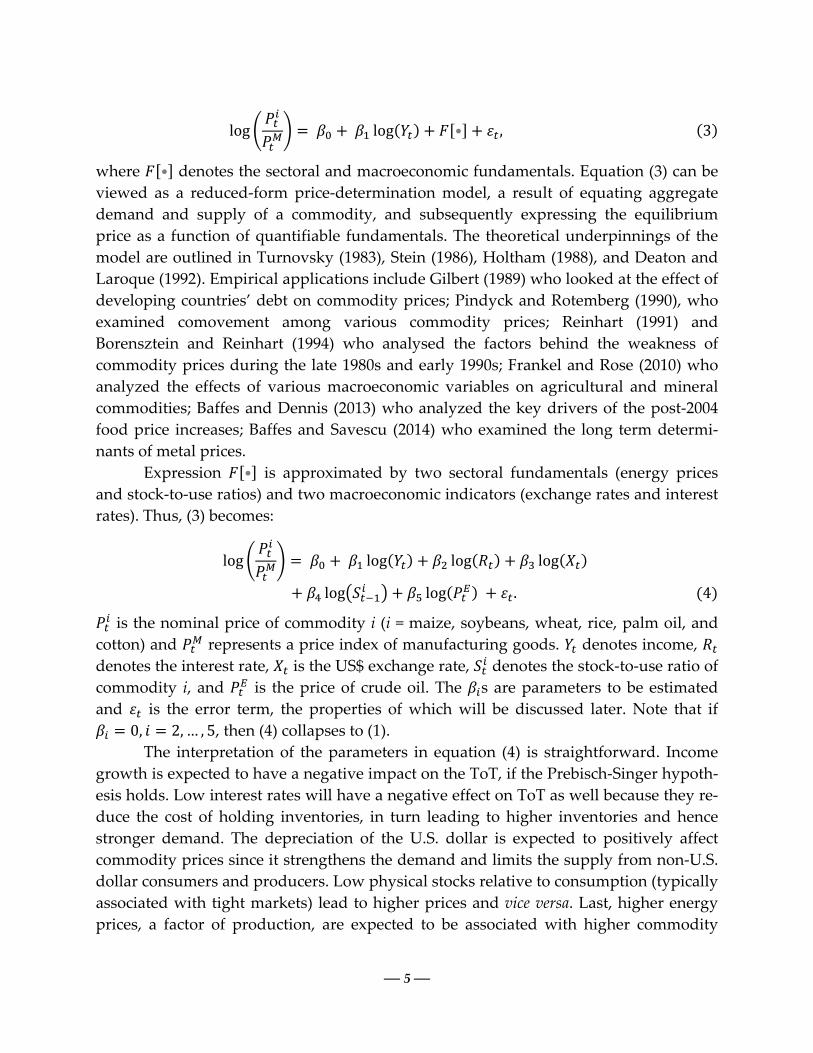
log log • , 3

where • denotes the sectoral and macroeconomic fundamentals. Equation (3) can be

viewed as a reduced-form price-determination model, a result of equating aggregate

demand and supply of a commodity, and subsequently expressing the equilibrium

price as a function of quantifiable fundamentals. The theoretical underpinnings of the

model are outlined in Turnovsky (1983), Stein (1986), Holtham (1988), and Deaton and

Laroque (1992). Empirical applications include Gilbert (1989) who looked at the effect of

developing countries’ debt on commodity prices; Pindyck and Rotemberg (1990), who

examined comovement among various commodity prices; Reinhart (1991) and

Borensztein and Reinhart (1994) who analysed the factors behind the weakness of

commodity prices during the late 1980s and early 1990s; Frankel and Rose (2010) who

analyzed the effects of various macroeconomic variables on agricultural and mineral

commodities; Baffes and Dennis (2013) who analyzed the key drivers of the post-2004

food price increases; Baffes and Savescu (2014) who examined the long term determi-

nants of metal prices.

Expression • is approximated by two sectoral fundamentals (energy prices

and stock-to-use ratios) and two macroeconomic indicators (exchange rates and interest

rates). Thus, (3) becomes:

log log log log

log log . 4

is the nominal price of commodity i (i = maize, soybeans, wheat, rice, palm oil, and

cotton) and represents a price index of manufacturing goods. denotes income,

denotes the interest rate, is the US$ exchange rate, denotes the stock-to-use ratio of

commodity i, and is the price of crude oil. The s are parameters to be estimated

and is the error term, the properties of which will be discussed later. Note that if

0, 2, … , 5, then (4) collapses to (1).

The interpretation of the parameters in equation (4) is straightforward. Income

growth is expected to have a negative impact on the ToT, if the Prebisch-Singer hypoth-

esis holds. Low interest rates will have a negative effect on ToT as well because they re-

duce the cost of holding inventories, in turn leading to higher inventories and hence

stronger demand. The depreciation of the U.S. dollar is expected to positively affect

commodity prices since it strengthens the demand and limits the supply from non-U.S.

dollar consumers and producers. Low physical stocks relative to consumption (typically

associated with tight markets) lead to higher prices and vice versa. Last, higher energy

prices, a factor of production, are expected to be associated with higher commodity

— 6 —

prices.4 Hence, the expected signs of the parameter estimates (noted as superscripts) are: , , , , .

For the second objective, that is, identifying the channel through which income

affects ToT, we relax the homogeneity assumption of manufacturing prices and re-

parameterize (4) as follows:

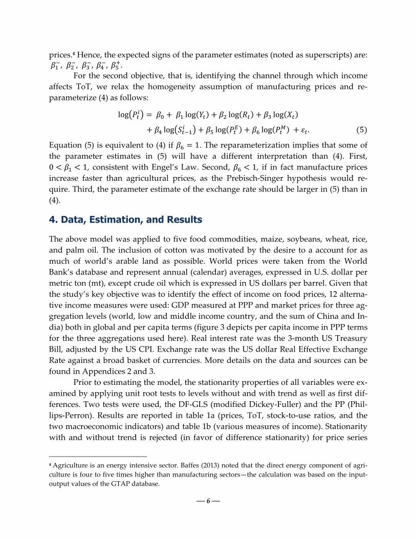
log log log log

log log log . 5

Equation (5) is equivalent to (4) if 1. The reparameterization implies that some of

the parameter estimates in (5) will have a different interpretation than (4). First,

0 1, consistent with Engel’s Law. Second, 1, if in fact manufacture prices

increase faster than agricultural prices, as the Prebisch-Singer hypothesis would re-

quire. Third, the parameter estimate of the exchange rate should be larger in (5) than in

(4).

4. Data, Estimation, and Results

The above model was applied to five food commodities, maize, soybeans, wheat, rice,

and palm oil. The inclusion of cotton was motivated by the desire to a account for as

much of world’s arable land as possible. World prices were taken from the World

Bank’s database and represent annual (calendar) averages, expressed in U.S. dollar per

metric ton (mt), except crude oil which is expressed in US dollars per barrel. Given that

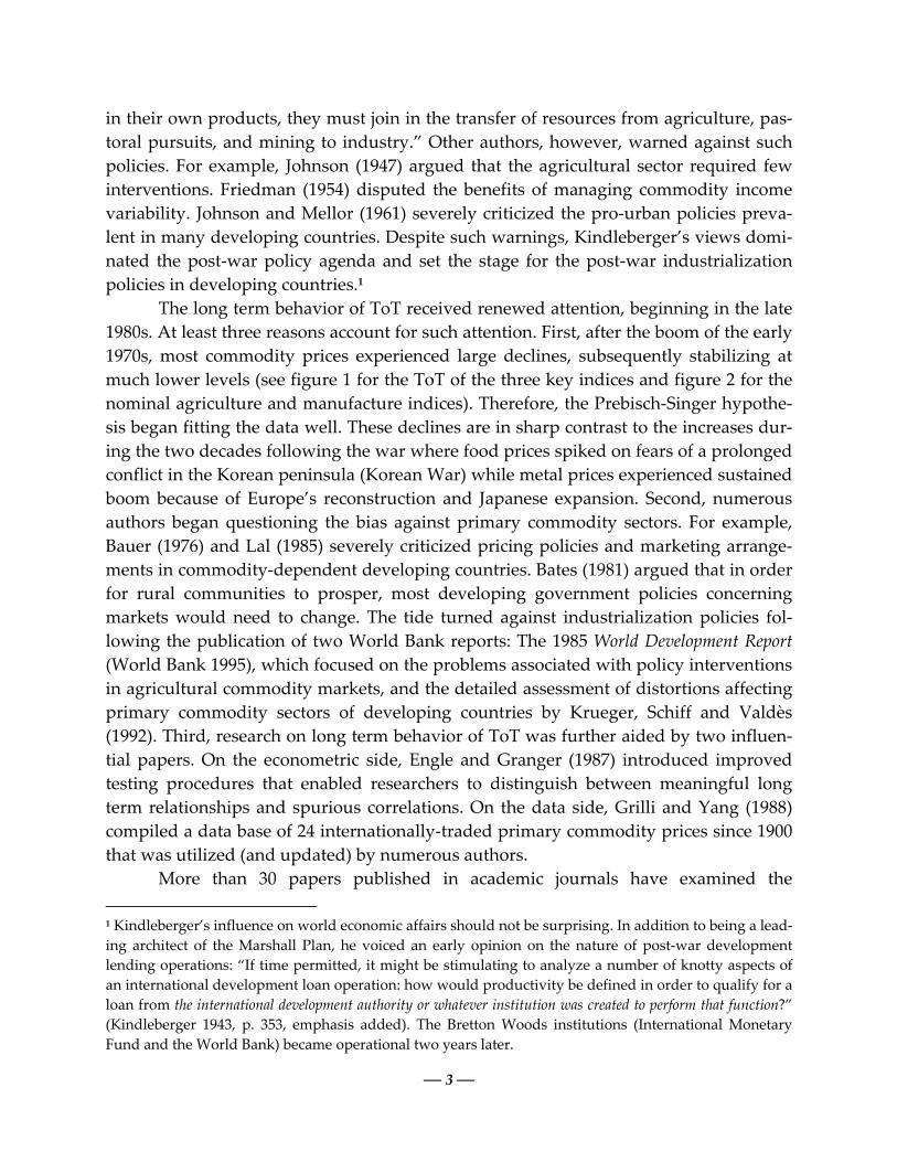
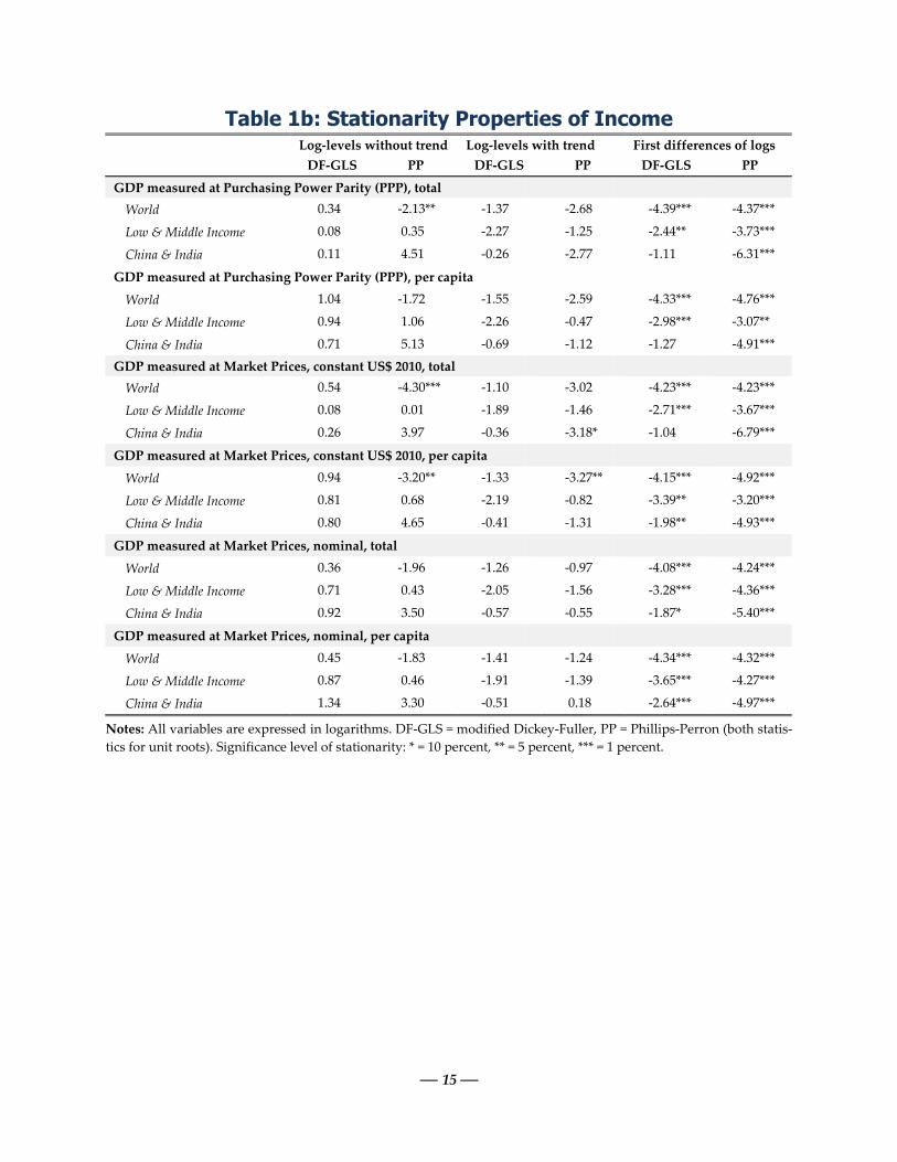
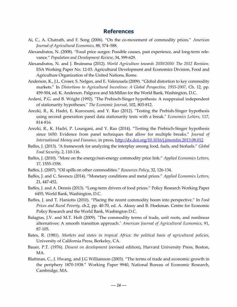
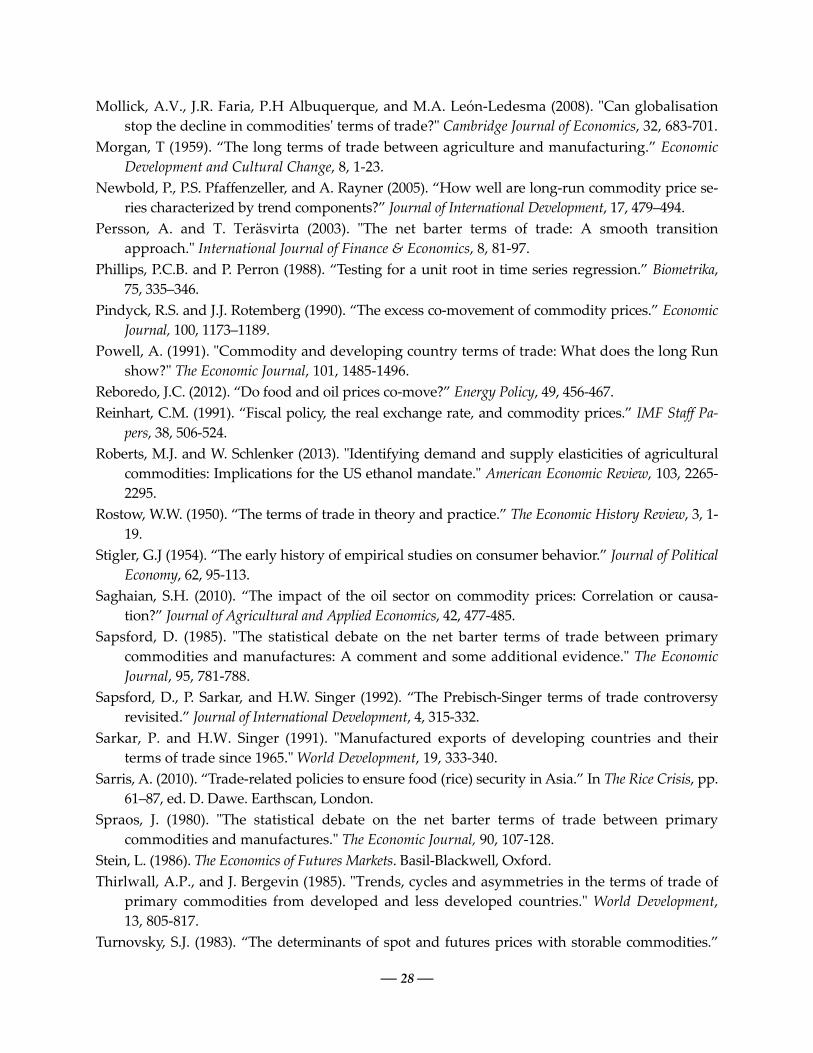
the study’s key objective was to identify the effect of income on food prices, 12 alterna-

tive income measures were used: GDP measured at PPP and market prices for three ag-

gregation levels (world, low and middle income country, and the sum of China and In-

dia) both in global and per capita terms (figure 3 depicts per capita income in PPP terms

for the three aggregations used here). Real interest rate was the 3-month US Treasury

Bill, adjusted by the US CPI. Exchange rate was the US dollar Real Effective Exchange

Rate against a broad basket of currencies. More details on the data and sources can be

found in Appendices 2 and 3.

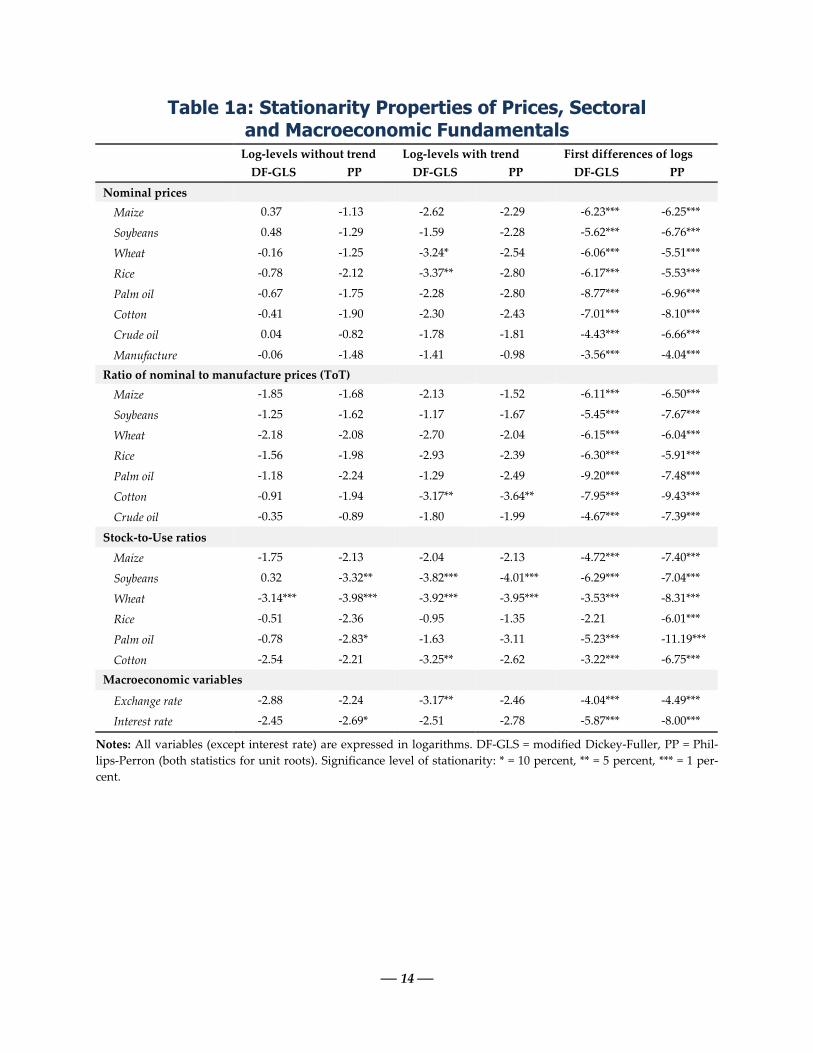
Prior to estimating the model, the stationarity properties of all variables were ex-

amined by applying unit root tests to levels without and with trend as well as first dif-

ferences. Two tests were used, the DF-GLS (modified Dickey-Fuller) and the PP (Phil-

lips-Perron). Results are reported in table 1a (prices, ToT, stock-to-use ratios, and the

two macroeconomic indicators) and table 1b (various measures of income). Stationarity

with and without trend is rejected (in favor of difference stationarity) for price series

4 Agriculture is an energy intensive sector. Baffes (2013) noted that the direct energy component of agri-

culture is four to five times higher than manufacturing sectors—the calculation was based on the input-

output values of the GTAP database.

— 7 —

regardless of whether they are expressed in nominal or ToT form.5 With the exception

of wheat (and less so soybeans), difference stationarity is confirmed for the S/U ratio

and the two macroeconomic indicators. Similar results hold for the various measures of

income.6 Thus, on the basis of unit root statistics, the performance of the models should

be judged by the stationarity properties of the error term, in addition to conventional

measures.

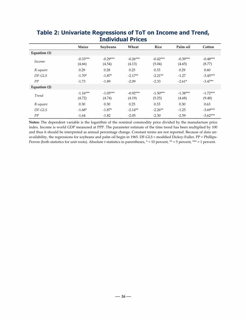
Setting the Stage We begin with a univariate regression for the ToT of the six commodities against in-

come, which is the simplest way to test the Prebisch-Singer hypothesis. The results (re-

ported in the upper panel of table 2) show that the parameter estimate of income was

negative and significantly different from zero at the 1 percent level in all six cases, with

the estimates ranging from -0.26 for wheat to -0.48 for cotton. Such result is consistent

with the Prebisch-Singer hypothesis. Moreover, with the exception of cotton, evidence

in favor of cointegration is weak, implying that income alone does not explain commod-

ity price trends. The lower panel of table 2 reports results of the price ToT on time

trend. Again, the results are remarkably similar to those of income: Negative parameter

estimate of trend with the highest and lowest for cotton and wheat, respectively along

with very weak evidence of trend stationarity, with the exception of cotton. These re-

sults, point to the following conclusions: However, the evidence on food commodities is in favor of the Prebisch-Singer hypothesis.

However, on the basis of the explanatory power (R-square) and stationarity statistics, income or

time trend alone cannot adequately explain commodity price movements.

Apart from the individual price ToT, we run the same regression for six com-

modity price indices: food (which contain the food prices used in the model), raw mate-

rials, beverages, energy, industrial metals, and precious metals. The results (reported in

5 Beyond their importance for the subsequent econometric analysis, rejection of stationarity and trend

stationarity of both nominal prices and ToT, implies that comovement between nominal food and manu-

facture prices (with unity cointegration parameter) is rejected as well, another (albeit much stricter) test

for the Prebisch-Singer hypothesis. Even more importantly, nonstationarity of prices highlights the prac-

tical difficulties with price stabilization mechanisms. Consider, for example, that the ToT for agriculture

has fluctuated between a high of 149 in 1974 (2010 = 100) and a low of 61 in 2001. More interestingly, the

path has crossed its mean, 92, only four times, three of which occurred during 1981-85. Thus, for a long

term price stabilization mechanism to work, a policy maker would have to “tax” the sector during 1960-

1981 and “subsidize” it during 1985-2008. These, admittedly simplistic, calculations point to the impossi-

bility of devising meaningful price stabilization mechanisms.

6 Of the 36 tests for stationarity for levels with trend and another 36 for levels with trend, the null of no

unit root was rejected in only 3 cases at the 5 percent level of significance. Similarly, of the 36 unit root

tests in first differences, in only 4 cases stationarity was rejected at the 5 percent level (all 4 were for DF-

GLS for India & China GDP). Thus, only seven out of 108 cases (6.5 percent) are not consistent with dif-

ference stationarity, remarkably close to the 5 percent level of significant.

— 8 —

the upper panel of table 3) give a mixed picture. The effect of income on the food, bev-

erage, and (less so) raw materials index ToT is negative and significantly different from

zero. It is virtually zero for metals and large, but positive and highly significant for en-

ergy and precious metals. Furthermore, the unit root statistics indicate very weak evi-

dence of cointegration between commodity indices ToT and income. The lower panel of

table 3 reports univariate regression results on a time trend with remarkably similar re-

sults.

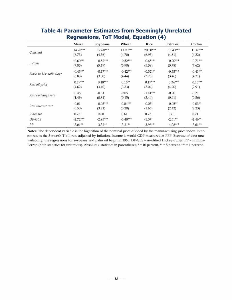
The Role of Income Table 4 reports parameter estimates consistent with equation (4). For efficiency gains,

the model was estimated as a system of seemingly unrelated regressions (SUR). The

models performed in a satisfactory manner. For example, 23 out of 30 parameter esti-

mates (excluding the β0) were significantly different from zero at the 5 percent level.

Furthermore, more than two thirds of price variability is explained by the fundamentals

and, with the single exception of the DF-GLS statistics for rice, the error term is station-

ary in all models. In all cases income had a negative and significantly different from ze-

ro parameter estimate (at the 1 percent level). The estimates range within a remarkably

tight band, from -0.52 for soybeans and rice (t-statistic = -5.19 & -5.50) to -0.71 for cotton

(t-statistic = -7.62).

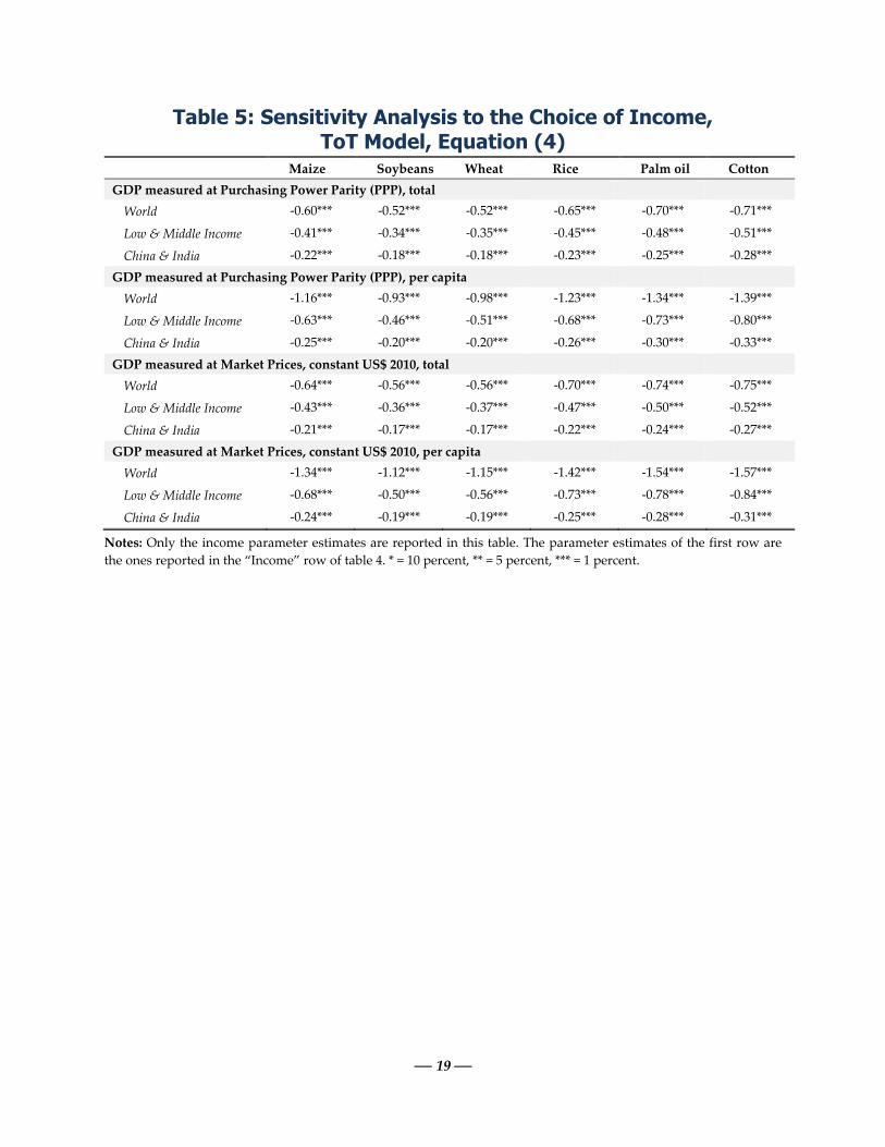
In addition to the income measure reported in table 4 (world GDP evaluated at

Purchasing Power Parity), equation (4) was re-estimated by using the 12 income

measures discussed earlier, again using SUR. Parameter estimates are reported in table

5 (to conserve space, only the income parameter estimate is reported.) The parameter

estimate of income was negative and significantly different from zero at the 1 percent

level for all 12 income measures and 6 commodity prices. Three key conclusions emerge

from these results: Results reported in table 4 and 5 confirm the Prebisch-Singer hypothesis for food commodity

prices—consistent with the univariate model.

The univariate models underestimate the negative impact of income of ToT by almost half.

The unit root-free error terms imply that fundamentals adequately explain the behavior of ToT.

These results hold regardless of the measure of income used.

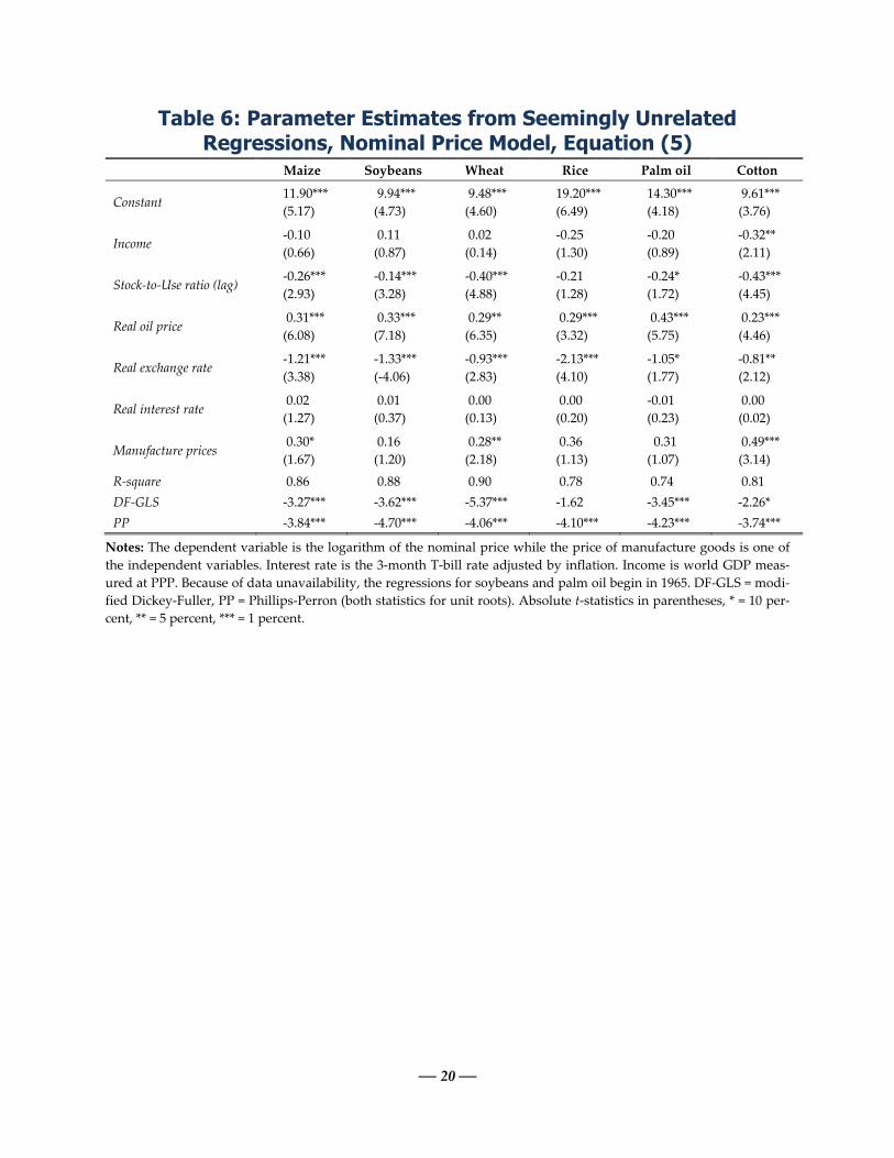
Yet, it is not clear whether income’s negative impact on ToT operates through

nominal commodity prices, , manufacture prices, , or both. To identify the trans-

mission channel, we estimate equation (5), results are of which are reported in table 6.

On the basis of the explanatory power and stationarity statistics, the nominal price

model appears to have performed much better than the ToT model.7 The R-square aver- 7 The superior performance of (5) should not be surprising because of the relaxation of the homogeneity

restriction imposed on the parameter estimate of . In fact, Houthakker (1975) argued in favor of relax-

ing such restriction on the deflator because, in addition to improving the model’s performance, the im-

pact of fundamentals on nominal prices can be assessed in a direct fashion.

— 9 —

aged 0.83, up from 0.67 in the ToT model while 10 out of 12 unit root tests confirmed

stationarity of the error term at the 1 percent level of significance—as before, exception

is the DF-GLS test for rice.

In no case income had a positive effect on nominal prices; for the five food com-

modity prices, the parameter estimate was not significantly different from zero while

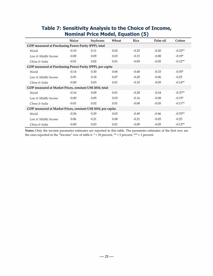
for cotton the estimate was negative and significant at the 5 percent level. As in the ToT

case the model was replicated with all 12 measures of income (results are reported in

table 7). Again, with the exception of cotton where in 7 cases the parameter estimate of

income was negative and significantly different from zero at the 5 percent level, income

appears to have no effect on nominal prices. These results point to the following conclu-

sions. Income exerted no effect on nominal prices (with the single exception of cotton where the effect

was negative), a result which is consistent with Engel’s Law.

Thus, the negative effect of income on ToT derived earlier is transmitted through manufacture,

not primary, commodity prices.

The parameter estimate of the manufacture prices is far less than unity in three cases (maize,

wheat, cotton) and zero in the remaining cases, implying that the homogeneity condition is a very

restrictive assumption. This is also evident by the explanatory power and improved cointegration

statistics of the nominal price model.

Although these results are in sharp contrast to what has been assumed or report-

ed in the literature, they should not come as surprise. If income had a strong positive

effect on food prices, that should have showed up on consumption patterns. Yet, evi-

dence that grain consumption by emerging economies has experienced growth rates

that are either high by historical standards or comparable to their income growth rates

is, at best, weak. Alexandratos (2008, p. 673) concluded that China’s and India’s com-

bined average annual increment in grain consumption was lower in 2002-08 than in

1995-2001. In a similar vein, FAO (2008, p. 12) noted that:

China and India have usually been cited as the main contributors to this sudden

change [in cereal prices] because of the size of their populations and the high

rates of economic growth they have achieved. However, since 1980, the imports

of cereals in these two countries have been trending down, on average by 4 per-

cent per year, from an average of 14.4 million tonnes in the early 1980s to 6.3 mil-

lion tonnes over the past three years. Moreover, mainland China has been a net

exporter of cereals since the late-1990s, with one exception in the 2004-05 season.

Similarly, India has been a net importer of these commodities only once, in the

2006-07 season, since the beginning of the twenty-first century.

Numerous other studies have reported similar findings, including Alexandratos and

Bruinsma (2012), Sarris (2010), Baffes and Haniotis (2010), FAO (2009), and Lustig

(2008). In fact, Deaton and Drèze (2008), based on household survey data in India found

that, despite growing incomes, there has been a downward trend in calorie intake since

— 10 —

the early 1990s. They added that although the reasons behind this trend are not clear,

one likely explanation may be that calorie requirements have declined as a result of bet-

ter health and lower physical activity levels.

The Role of Sectoral Fundamentals The discussion thus far focused on income. Yet, as evidenced by the models, it is the

remaining fundamentals that play a key role in the food price determination process. As

expected the stock-to-use ratio estimates are negative and highly significant, ranging

from a high of -0.43 for maize to a low of -0.17 for soybeans. The nominal price model

(table 6) gave similar estimates, except rice, whose estimate was not significantly differ-

ent from zero. The stock-to-use ratio elasticities estimates for the three grains reported

here are remarkably similar to findings reported elsewhere. For example, Bobenrieth,

Wright, and Zeng (2012) estimated correlation coefficients between stock-to-use ratios

and real de-trended prices for wheat, maize, and rice of -0.40, -0.50, and -0.17, respec-

tively (compared to -0.42, -0.43, and -0.32 from the ToT model or -0.26, -0.40, -0.21 from

the nominal price model.)8 Similarly, FAO (2008, p. 6, figure 3) reported correlation co-

efficients between the cereals price index and various measures of stock-to-use ratios

ranging from -0.47 and -0.65.

The estimate of the oil price elasticity was different from zero in all six regres-

sions in both specifications—the only parameter estimate significantly different from

zero at the 5 percent level across the two versions of the 6 models. The oil elasticity av-

eraged 0.20 in the ToT model and 0.31 in the nominal price model, implying that a dou-

bling in oil prices would lead to a 20 to 30 percent increase in food prices. In both mod-

els the lowest estimate was for cotton (0.15, t-statistic = 2.91 and 0.23, t-statistic = 4.46)

and the highest was for palm oil (0.34, t-statistic = 4.70 and 0.43, t-statistic = 5.75).

The strong relationship between energy and non-energy prices has been estab-

lished long before the post-2004 price boom. Gilbert (1989), for example, using quarterly

data between 1965 and 1986, estimated transmission elasticity from energy to non-

energy commodities of 0.12 and from energy to food commodities of 0.25. Hanson et al.

(1993) based on a General Equilibrium Model found a significant effect of oil price

changes to agricultural producer prices in the United States. Borensztein and Reinhart

(1994), using quarterly data from 1970 to 1992, estimated transmission elasticity to non-

8 The low and not significantly different from zero for rice (nominal price model) most likely reflects poli-

cy distortions, including the substantial quantities of rice stocks that are either handled by state trading

enterprises or heavily influenced by government policies (Alavi and others 2012). Indeed, Anderson and

others (2009, p. 489, table 12.11) estimated that during 2000-04, rice exhibited the highest level of distor-

tion (43 percent) compared to wheat (4 percent) and maize (3 percent), as measured by the trade restric-

tiveness index. Martin and Anderson (2012, p. 426) found that restrictive trade policies during the 2006-08

price spike may explain as much as 45 percent of the increase in the international rice price.

— 11 —

energy commodities of 0.11. A strong relationship between energy and non-energy

prices was found by Chaudhuri (2001) as well. Baffes (2007), using annual data from

1960 to 2005 estimated elasticities of 0.16 and 0.18 for non-energy and food commodi-

ties, respectively. In a similar model that included the recent boom, Baffes (2010) report-

ed somewhat higher elasticities. Moss et al. (2010) found that U.S. agriculture’s energy

demand is more sensitive to price changes than any other input.

Yet not all studies concur with a strong oil/non-oil price relationship. Saghaian

(2010) established strong correlation among oil and other commodity prices (including

food) but the evidence for a causal link from oil to other commodities was mixed. Gil-

bert (2010) found a correlation between the oil price and food prices both in terms of

levels and changes, but also noted that it is the result of common causation and not of a

direct causal link. Zhang et al. (2010) found no direct long-run relationship between fuel

and agricultural commodity prices and only a limited short-run relationship. Reboredo

(2012) concluded that the prices of maize, wheat, and soybeans are not driven by oil

price fluctuations. Baffes (2013) noted that, in the presence of biofuels, the mixed evi-

dence on the energy/non-energy price relationship should not be surprising. To see this,

consider an exogenous shock which pushes crude oil prices up, in turn, lowering fuel

consumption. Under a mandated ethanol/gasoline mixture ethanol and maize prices

will decline, ceteris paribus, leading to a negative relationship between food and oil pric-

es (De Gorter and Just 2008). The mixed evidence on the energy/non-energy price link

may also reflect the frequency of the data used in various models. Indeed, Zilberman et

al (2013) noted that higher frequency (and hence “noisier”) data are typically associated

with weaker correlations. The results on the effects of sectoral fundamentals on food

prices point to the following conclusions. Crude oil is the most important driver to food prices. An average elasticity of 0.25 implies that

the 200 percent increase in energy costs during the past decade could explain more than half of

the food price increases.

While crop conditions, as reflected by the stock-to-use ratios, had significant effect on food prices

(the elasticity estimate was almost twice as high compared to crude oil), the actual effect is much

smaller because the stock-to-use ratios changed much less during the boom period.

The Role of Macroeconomic Indicators Results of the effect of the exchange rate on food prices are mixed but they are highly

consistent with expectations. The parameter estimates from the nominal price model

(table 6), which are all significantly different from zero, indicate that exchange rates

matter a lot, especially in rice whose estimate is twice as high compared to other prices

(-2.13, t-statistic = -4.10). The large parameter estimate for rice is consistent with initial

expectations given that the United States does not play any significant role in that mar-

ket. These results are line with earlier literature. See, for example, Lamm (1980), Gard-

ner (1981), and Baffes and Dennis (2013) for agriculture and Gilbert (1989), Baffes (1997),

— 12 —

and Akram (2009) for metals. Estimates from the ToT model, however, indicate a con-

siderably weaker effect of exchange rate (except rice.) Again, this outcome is expected

since ToT is a currency-free unit.

Last, the results on the effect of interest rates on the ToT are mixed. Wheat had a

positive and significantly different from zero parameter estimates for soybeans, palm

oil, and cotton, the estimate was negative and significant, and zero for maize. Again, the

mixed nature of the interest rate results is consistent with the literature on the subject.

Gilbert (1989) based on an error-correction model (1965Q1–1986Q2) concluded that high

interest rates have a negative impact on the metal price index, though with considerable

lags. Baffes (1997), who used a reduced form price model for five metals (1971Q1–

1988Q4) estimated mostly negative but not significantly different from zero elasticities.

Akram (2009), based on a VAR model (1990Q1–2007Q4), concluded that commodity

prices (including metals) increase significantly in response to reduction in real interest

rates. Anzuini et al. (2010), who applied a VAR on monthly data for 1970–2009, did es-

tablish that easy monetary policy is associated with higher commodity prices but also

noted that the impact is modest. Frankel and Rose (2010) based on annual data for a

number of commodities found little support that easy monetary policy and low real in-

terest rates are an important source of upward pressure on real commodity prices. Last,

the 2013 Spillover Report (IMF, 2013) estimated that under a smooth growth-driven

normalization of monetary policy, a 100 basis points increase in short term interest rates

by the US Federal Reserve will lead to a 7% and 5% increase in energy and non-energy

commodity prices (under other scenarios, however, commodity prices would decline).

Based on the nominal price model, however, even this mixed evidence of the real ex-

change rate weakens further, implying that, as it was the case with income, the interest

rate effect operates through the manufacture, not the primary commodity, price chan-

nel. The results on the effects of macroeconomic fundamentals can be summarized as

follows. The US dollar depreciation positively affects nominal food prices, as expected; with a single excep-

tion of rice, there is no exchange rate effect on the ToT, since the latter is currency-free unit.

The effect of interest rate on the ToT is small and mixed. There is no interest rate impact on nom-

inal prices, however, implying that even the limited impact, operates through manufacture prices.

5. Summary and Conclusion

This paper reconciled the Prebisch-Singer hypothesis—which states that the ratio of

primary commodity prices over manufacture prices declines as income increases—with

the recently held view that income growth by emerging economies has been a key driv-

er of the food price increases during the past 10 years. In particular, the paper extended

the literature on the Prebisch-Singer hypothesis in three ways. First, it tested the hy-

pothesis by examining the effect of income on the ToT, as originally envisaged by

— 13 —

Kindleberger, rather than relating ToT with time, which is the common practice in the

literature. Second, in addition to income, the model accounted for the key sectoral and

macroeconomic fundamentals that are expected to influence commodity prices. Third,

the model examined whether the income effect on ToT operates through primary com-

modity prices, manufacturing prices or both.

The paper employed a reduced-form price determination model and applied it to

1960-2013 annual data for five food commodities (maize, soybeans, wheat, rice, palm

oil) and cotton. It concluded that income has a negative and highly significant effect on

real agricultural commodity prices. This finding is consistent with and Engel’s Law and

Kindleberger’s thesis, the predecessor of the Prebisch-Singer hypothesis. Moreover, it is

shown that income’s negative impact on real prices operates through the manufacturing

price channel (the deflator), thus, weakening the view that income growth by emerging

economies has played a major role during the past decade’s run up in food prices. Other

key drivers include (in order of importance) the role of energy costs, physical stocks,

and monetary conditions.

On the methodological side, the literature review showed that the research on

the Prebisch-Singer hypothesis reflects mostly concerns of primary commodity prices

not manufacturing prices. Yet, this paper showed that the negative impact of income

(and interest rates) operates mostly through the manufacturing price channel, not the

primary commodity price channel.

— 14 —

Table 1a: Stationarity Properties of Prices, Sectoral and Macroeconomic Fundamentals

Log-levels without trend Log-levels with trend First differences of logs

DF-GLS PP DF-GLS PP DF-GLS PP

Nominal prices

Maize 0.37 -1.13 -2.62 -2.29 -6.23*** -6.25***

Soybeans 0.48 -1.29 -1.59 -2.28 -5.62*** -6.76***

Wheat -0.16 -1.25 -3.24* -2.54 -6.06*** -5.51***

Rice -0.78 -2.12 -3.37** -2.80 -6.17*** -5.53***

Palm oil -0.67 -1.75 -2.28 -2.80 -8.77*** -6.96***

Cotton -0.41 -1.90 -2.30 -2.43 -7.01*** -8.10***

Crude oil 0.04 -0.82 -1.78 -1.81 -4.43*** -6.66***

Manufacture -0.06 -1.48 -1.41 -0.98 -3.56*** -4.04***

Ratio of nominal to manufacture prices (ToT)

Maize -1.85 -1.68 -2.13 -1.52 -6.11*** -6.50***

Soybeans -1.25 -1.62 -1.17 -1.67 -5.45*** -7.67***

Wheat -2.18 -2.08 -2.70 -2.04 -6.15*** -6.04***

Rice -1.56 -1.98 -2.93 -2.39 -6.30*** -5.91***

Palm oil -1.18 -2.24 -1.29 -2.49 -9.20*** -7.48***

Cotton -0.91 -1.94 -3.17** -3.64** -7.95*** -9.43***

Crude oil -0.35 -0.89 -1.80 -1.99 -4.67*** -7.39***

Stock-to-Use ratios

Maize -1.75 -2.13 -2.04 -2.13 -4.72*** -7.40***

Soybeans 0.32 -3.32** -3.82*** -4.01*** -6.29*** -7.04***

Wheat -3.14*** -3.98*** -3.92*** -3.95*** -3.53*** -8.31***

Rice -0.51 -2.36 -0.95 -1.35 -2.21 -6.01***

Palm oil -0.78 -2.83* -1.63 -3.11 -5.23*** -11.19***

Cotton -2.54 -2.21 -3.25** -2.62 -3.22*** -6.75***

Macroeconomic variables

Exchange rate -2.88 -2.24 -3.17** -2.46 -4.04*** -4.49***

Interest rate -2.45 -2.69* -2.51 -2.78 -5.87*** -8.00***

Notes: All variables (except interest rate) are expressed in logarithms. DF-GLS = modified Dickey-Fuller, PP = Phil-

lips-Perron (both statistics for unit roots). Significance level of stationarity: * = 10 percent, ** = 5 percent, *** = 1 per-

cent.

— 15 —

Table 1b: Stationarity Properties of Income Log-levels without trend Log-levels with trend First differences of logs

DF-GLS PP DF-GLS PP DF-GLS PP

GDP measured at Purchasing Power Parity (PPP), total

World 0.34 -2.13** -1.37 -2.68 -4.39*** -4.37***

Low & Middle Income 0.08 0.35 -2.27 -1.25 -2.44** -3.73***

China & India 0.11 4.51 -0.26 -2.77 -1.11 -6.31***

GDP measured at Purchasing Power Parity (PPP), per capita

World 1.04 -1.72 -1.55 -2.59 -4.33*** -4.76***

Low & Middle Income 0.94 1.06 -2.26 -0.47 -2.98*** -3.07**

China & India 0.71 5.13 -0.69 -1.12 -1.27 -4.91***

GDP measured at Market Prices, constant US$ 2010, total

World 0.54 -4.30*** -1.10 -3.02 -4.23*** -4.23***

Low & Middle Income 0.08 0.01 -1.89 -1.46 -2.71*** -3.67***

China & India 0.26 3.97 -0.36 -3.18* -1.04 -6.79***

GDP measured at Market Prices, constant US$ 2010, per capita

World 0.94 -3.20** -1.33 -3.27** -4.15*** -4.92***

Low & Middle Income 0.81 0.68 -2.19 -0.82 -3.39** -3.20***

China & India 0.80 4.65 -0.41 -1.31 -1.98** -4.93***

GDP measured at Market Prices, nominal, total

World 0.36 -1.96 -1.26 -0.97 -4.08*** -4.24***

Low & Middle Income 0.71 0.43 -2.05 -1.56 -3.28*** -4.36***

China & India 0.92 3.50 -0.57 -0.55 -1.87* -5.40***

GDP measured at Market Prices, nominal, per capita

World 0.45 -1.83 -1.41 -1.24 -4.34*** -4.32***

Low & Middle Income 0.87 0.46 -1.91 -1.39 -3.65*** -4.27***

China & India 1.34 3.30 -0.51 0.18 -2.64*** -4.97***

Notes: All variables are expressed in logarithms. DF-GLS = modified Dickey-Fuller, PP = Phillips-Perron (both statis-

tics for unit roots). Significance level of stationarity: * = 10 percent, ** = 5 percent, *** = 1 percent.

— 16 —

Table 2: Univariate Regressions of ToT on Income and Trend, Individual Prices

Maize Soybeans Wheat Rice Palm oil Cotton

Equation (1)

Income -0.33***

(4.66)

-0.29***

(4.54)

-0.26***

(4.13)

-0.42***

(5.04)

-0.39***

(4.65)

-0.48***

(8.77)

R-square 0.29 0.28 0.25 0.33 0.29 0.60

DF-GLS -1.70* -1.87* -2.17** -2.21** -1.27 -3.45***

PP -1.73 -1.89 -2.09 -2.33 -2.61* -3.47**

Equation (2)

Trend -1.16***

(4.72)

-1.05***

(4.74)

-0.92***

(4.19)

-1.50***

(5.25)

-1.38***

(4.68)

-1.72***

(9.48)

R-square 0.30 0.30 0.25 0.33 0.30 0.63

DF-GLS -1.68* -1.87* -2.14** -2.26** -1.25 -3.69***

PP -1.64 -1.82 -2.05 -2.30 -2.59 -3.62***

Notes: The dependent variable is the logarithm of the nominal commodity price divided by the manufacture price

index. Income is world GDP measured at PPP. The parameter estimate of the time trend has been multiplied by 100

and thus it should be interpreted as annual percentage change. Constant terms are not reported. Because of data un-

availability, the regressions for soybeans and palm oil begin in 1965. DF-GLS = modified Dickey-Fuller, PP = Phillips-

Perron (both statistics for unit roots). Absolute t-statistics in parentheses, * = 10 percent, ** = 5 percent, *** = 1 percent.

— 17 —

Table 3: Univariate Regressions of ToT on Income and Trend, Price Indices

Food Raw

Materials Beverages Energy Metals

Precious

Metals

Equation (1)

Income -0.27***

(4.53)

-0.10**

(2.63)

-0.38***

(4.89)

1.29***

(11.22)

-0.00

(0.01)

0.75***

(8.48)

R-square 0.28 0.12 0.32 0.71 0.00 0.58

DF-GLS -0.89 -1.26 -2.26** -1.84* -1.94* -2.23**

PP -1.56 -1.73* -2.41 -2.09 -1.89 -1.78

Equation (2)

Trend -0.94***

(4.67)

-0.29**

(2.19)

-1.41***

(5.40)

-4.33***

(10.21)

0.01

(0.04)

2.51***

(7.79)

R-square 0.30 0.08 0.36 0.67 0.00 0.54

DF-GLS -1.88 -2.75* -2.32** -1.81** -1.94* -2.16*

PP -1.49 -1.89 -2.47 -1.91 -1.89 -1.72

Notes: The dependent variable is the logarithm of the nominal commodity the nominal price index divided by the

manufacture price index. Income is world GDP measured at PPP. The parameter estimate of the time trend has been

multiplied by 100 and thus it should be interpreted as annual percentage change. Constant terms are not reported.

DF-GLS = modified Dickey-Fuller, PP = Phillips-Perron (both statistics for unit roots). Absolute t-statistics in paren-

theses, * = 10 percent, ** = 5 percent, *** = 1 percent.

— 18 —

Table 4: Parameter Estimates from Seemingly Unrelated Regressions, ToT Model, Equation (4)

Maize Soybeans Wheat Rice Palm oil Cotton

Constant 14.70***

(6.73)

12.60***

(4.56)

11.90***

(4.70)

20.60***

(6.95)

16.40***

(4.81)

11.40***

(4.32)

Income -0.60***

(7.85)

-0.52***

(5.19)

-0.52***

(5.90)

-0.65***

(5.58)

-0.70***

(5.78)

-0.71***

(7.62)

Stock-to-Use ratio (lag) -0.43***

(6.83)

-0.17***

(3.00)

-0.42***

(4.44)

-0.32***

(3.75)

-0.35***

(3.46)

-0.41***

(4.31)

Real oil price 0.19***

(4.62)

0.18***

(3.40)

0.16**

(3.33)

0.17***

(3.04)

0.34***

(4.70)

0.15***

(2.91)

Real exchange rate -0.46

(1.49)

-0.31

(0.81)

-0.05

(0.15)

-1.41***

(3.44)

-0.20

(0.41)

-0.21

(0.56)

Real interest rate -0.01

(0.50)

-0.05***

(3.21)

0.04***

(3.20)

-0.03*

(1.66)

-0.05**

(2.42)

-0.03**

(2.23)

R-square 0.75 0.60 0.61 0.73 0.61 0.71

DF-GLS -2.72*** -2.95*** -3.48*** -1.57 -2.31** -2.46**

PP -3.01** -3.32** -3.21** -3.95*** -4.08*** -3.61***

Notes: The dependent variable is the logarithm of the nominal price divided by the manufacturing price index. Inter-

est rate is the 3-month T-bill rate adjusted by inflation. Income is world GDP measured at PPP. Because of data una-

vailability, the regressions for soybeans and palm oil begin in 1965. DF-GLS = modified Dickey-Fuller, PP = Phillips-

Perron (both statistics for unit roots). Absolute t-statistics in parentheses, * = 10 percent, ** = 5 percent, *** = 1 percent.

— 19 —

Table 5: Sensitivity Analysis to the Choice of Income, ToT Model, Equation (4)

Maize Soybeans Wheat Rice Palm oil Cotton

GDP measured at Purchasing Power Parity (PPP), total

World -0.60*** -0.52*** -0.52*** -0.65*** -0.70*** -0.71***

Low & Middle Income -0.41*** -0.34*** -0.35*** -0.45*** -0.48*** -0.51***

China & India -0.22*** -0.18*** -0.18*** -0.23*** -0.25*** -0.28***

GDP measured at Purchasing Power Parity (PPP), per capita

World -1.16*** -0.93*** -0.98*** -1.23*** -1.34*** -1.39***

Low & Middle Income -0.63*** -0.46*** -0.51*** -0.68*** -0.73*** -0.80***

China & India -0.25*** -0.20*** -0.20*** -0.26*** -0.30*** -0.33***

GDP measured at Market Prices, constant US$ 2010, total

World -0.64*** -0.56*** -0.56*** -0.70*** -0.74*** -0.75***

Low & Middle Income -0.43*** -0.36*** -0.37*** -0.47*** -0.50*** -0.52***

China & India -0.21*** -0.17*** -0.17*** -0.22*** -0.24*** -0.27***

GDP measured at Market Prices, constant US$ 2010, per capita

World -1.34*** -1.12*** -1.15*** -1.42*** -1.54*** -1.57***

Low & Middle Income -0.68*** -0.50*** -0.56*** -0.73*** -0.78*** -0.84***

China & India -0.24*** -0.19*** -0.19*** -0.25*** -0.28*** -0.31***

Notes: Only the income parameter estimates are reported in this table. The parameter estimates of the first row are

the ones reported in the “Income” row of table 4. * = 10 percent, ** = 5 percent, *** = 1 percent.

— 20 —

Table 6: Parameter Estimates from Seemingly Unrelated Regressions, Nominal Price Model, Equation (5)

Maize Soybeans Wheat Rice Palm oil Cotton

Constant 11.90***

(5.17)

9.94***

(4.73)

9.48***

(4.60)

19.20***

(6.49)

14.30***

(4.18)

9.61***

(3.76)

Income -0.10

(0.66)

0.11

(0.87)

0.02

(0.14)

-0.25

(1.30)

-0.20

(0.89)

-0.32**

(2.11)

Stock-to-Use ratio (lag) -0.26***

(2.93)

-0.14***

(3.28)

-0.40***

(4.88)

-0.21

(1.28)

-0.24*

(1.72)

-0.43***

(4.45)

Real oil price 0.31***

(6.08)

0.33***

(7.18)

0.29**

(6.35)

0.29***

(3.32)

0.43***

(5.75)

0.23***

(4.46)

Real exchange rate -1.21***

(3.38)

-1.33***

(-4.06)

-0.93***

(2.83)

-2.13***

(4.10)

-1.05*

(1.77)

-0.81**

(2.12)

Real interest rate 0.02

(1.27)

0.01

(0.37)

0.00

(0.13)

0.00

(0.20)

-0.01

(0.23)

0.00

(0.02)

Manufacture prices 0.30*

(1.67)

0.16

(1.20)

0.28**

(2.18)

0.36

(1.13)

0.31

(1.07)

0.49***

(3.14)

R-square 0.86 0.88 0.90 0.78 0.74 0.81

DF-GLS -3.27*** -3.62*** -5.37*** -1.62 -3.45*** -2.26*

PP -3.84*** -4.70*** -4.06*** -4.10*** -4.23*** -3.74***

Notes: The dependent variable is the logarithm of the nominal price while the price of manufacture goods is one of

the independent variables. Interest rate is the 3-month T-bill rate adjusted by inflation. Income is world GDP meas-

ured at PPP. Because of data unavailability, the regressions for soybeans and palm oil begin in 1965. DF-GLS = modi-

fied Dickey-Fuller, PP = Phillips-Perron (both statistics for unit roots). Absolute t-statistics in parentheses, * = 10 per-

cent, ** = 5 percent, *** = 1 percent.

— 21 —

Table 7: Sensitivity Analysis to the Choice of Income, Nominal Price Model, Equation (5)

Maize Soybeans Wheat Rice Palm oil Cotton

GDP measured at Purchasing Power Parity (PPP), total

World -0.10 0.11 0.02 -0.25 -0.20 -0.32**

Low & Middle Income -0.00 0.09 0.03 -0.15 -0.08 -0.19*

China & India -0.01 0.02 0.01 -0.09 -0.05 -0.12**

GDP measured at Purchasing Power Parity (PPP), per capita

World -0.14 0.30 0.06 -0.40 -0.33 -0.55*

Low & Middle Income 0.05 0.18 0.07 -0.20 -0.06 -0.25

China & India -0.00 0.03 0.01 -0.10 -0.05 -0.14**

GDP measured at Market Prices, constant US$ 2010, total

World -0.16 0.09 0.01 -0.28 -0.24 -0.37**

Low & Middle Income -0.00 0.09 0.03 -0.16 -0.08 -0.19*

China & India -0.01 0.02 0.01 -0.08 -0.05 -0.11**

GDP measured at Market Prices, constant US$ 2010, per capita

World -0.36 0.29 0.03 -0.49 -0.46 -0.70**

Low & Middle Income 0.06 0.21 0.08 -0.21 -0.05 -0.25

China & India -0.00 0.03 0.01 -0.09 -0.05 -0.13**

Notes: Only the income parameter estimates are reported in this table. The parameter estimates of the first row are

the ones reported in the “Income” row of table 6. * = 10 percent, ** = 5 percent, *** = 1 percent.

— 22 —

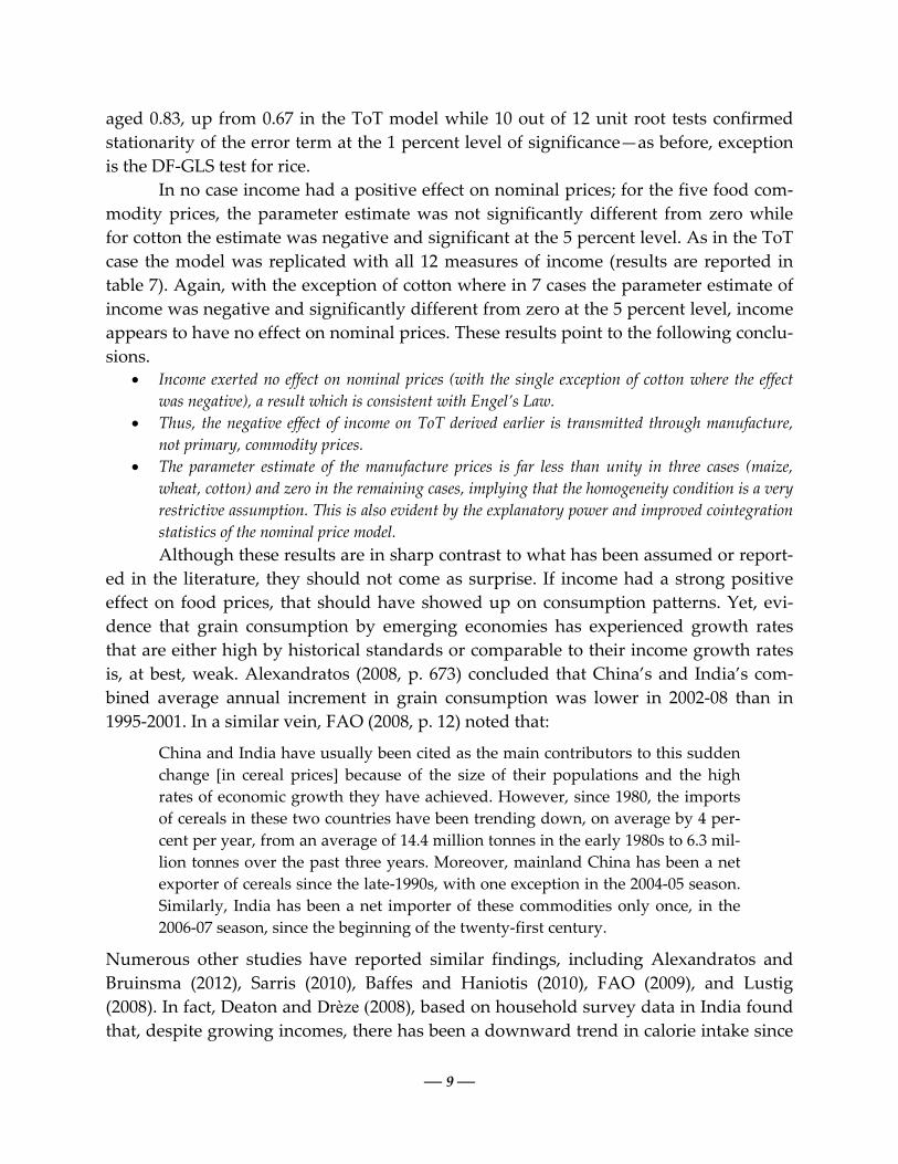
Figure 1 Commodity Prices (MUV-deflated, 2010 = 100)

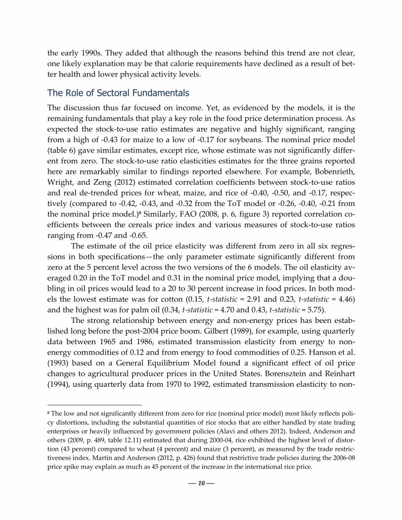
Figure 2 Agriculture and Manufacture Prices (Nominal, 2010 = 100)

-

20

40

60

80

100

120

140

160

180

1948 1953 1958 1963 1968 1973 1978 1983 1988 1993 1998 2003 2008 2013

Source: World Bank.

Agriculture

Metals

Energy

-

20

40

60

80

100

120

140

1960 1964 1968 1972 1976 1980 1984 1988 1992 1996 2000 2004 2008 2012

Source: World Bank

Agriculture

Manufacture

— 23 —

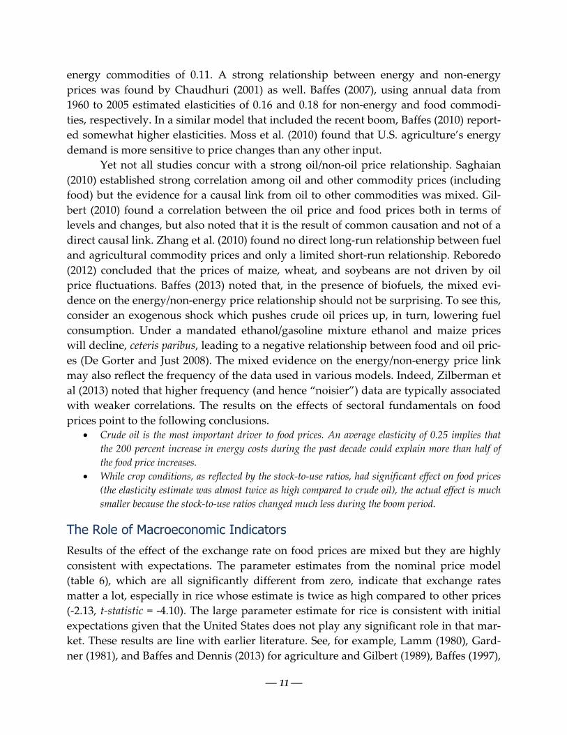
Figure 3 Per Capita Income measured at PPP

-

2,000

4,000

6,000

8,000

10,000

12,000

1961 1965 1969 1973 1977 1981 1985 1989 1993 1997 2001 2005 2009 2013

Low & middle income

Source: World Bank

China & India

World

— 24 —

References Ai, C., A. Chatrath, and F. Song (2006). “On the co-movement of commodity prices.” American

Journal of Agricultural Economics, 88, 574–588.

Alexandratos, N. (2008). “Food price surges: Possible causes, past experience, and long-term rele-

vance.” Population and Development Review, 34, 599-629.

Alexandratos, N. and J. Bruinsma (2012). World Agriculture towards 2030/2050: The 2012 Revision.

ESA Working Paper No. 12-03. Agricultural Development and Economics Division, Food and

Agriculture Organization of the United Nations, Rome.

Anderson, K., J.L. Croser, S. Nelgen, and E. Valenzuela (2009). “Global distortion to key commodity

markets.” In Distortions to Agricultural Incentives: A Global Perspective, 1955-2007, Ch. 12, pp.

459-504, ed. K. Anderson. Palgrave and McMillan for the World Bank, Washington, D.C.

Ardeni, P.G. and B. Wright (1992). "The Prebisch-Singer hypothesis: A reappraisal independent

of stationarity hypotheses." The Economic Journal, 102, 803-812.

Arezki, R., K. Hadri, E. Kurozumi, and Y. Rao (2012). "Testing the Prebish-Singer hypothesis

using second generation panel data stationarity tests with a break." Economics Letters, 117,

814-816.

Arezki, R., K. Hadri, P. Loungani, and Y. Rao (2014). “Testing the Prebisch-Singer hypothesis

since 1650: Evidence from panel techniques that allow for multiple breaks.” Journal of

International Money and Fianance, in press, http://dx.doi.org/10.1016/j.jimonfin.2013.08.012

Baffes, J. (2013). “A framework for analyzing the interplay among food, fuels, and biofuels.” Global

Food Security, 2, 110-116.

Baffes, J. (2010). “More on the energy/non-energy commodity price link.” Applied Economics Letters,

17, 1555-1558.

Baffes, J. (2007). “Oil spills on other commodities.” Resources Policy, 32, 126-134.

Baffes, J. and C. Savescu (2014). “Monetary conditions and metal prices.” Applied Economics Letters,

21, 447-452.

Baffes, J. and A. Dennis (2013). “Long-term drivers of food prices.” Policy Research Working Paper

6455, World Bank, Washington, D.C.

Baffes, J. and T. Haniotis (2010). “Placing the recent commodity boom into perspective.” In Food

Prices and Rural Poverty, ch.2, pp. 40-70, ed. A. Aksoy and B. Hoekman. Centre for Economic

Policy Research and the World Bank, Washington D.C.

Balagtas, J.V. and M.T. Holt (2009). "The commodity terms of trade, unit roots, and nonlinear

alternatives: A smooth transition approach." American Journal of Agricultural Economics, 91,

87-105.

Bates, R. (1981). Markets and states in tropical Africa: the political basis of agricultural policies,

University of California Press, Berkeley, CA.

Bauer, P.T. (1976). Dissent on development (revised edition), Harvard University Press, Boston,

MA.

Blattman, C., J. Hwang, and J.G Williamson (2003). “The terms of trade and economic growth in

the periphery 1870-1938.” Working Paper 9940, National Bureau of Economic Research,

Cambridge, MA.

— 25 —

Bleaney, M. and D. Greenaway (1993). "Long-run trends in the relative price of primary

commodities and in the terms of trade of developing countries." Oxford Economic Papers, 45,

349-363.

Bloch, H. and D. Sapsford (2000). "Whither the terms of trade? An elaboration of the Prebisch-

Singer hypothesis." Cambridge Journal of Economics, 24, 461-481.

Bobenrieth, E., B. Wright, and Z. Zeng (2012). “Stocks-to-Use ratios as indicator of vulnerability to

spikes in global cereal markets.” Paper presented at the Second Session of the Agricultural

Marketing Information System, Global Food Market Group. Food and Agriculture Organiza-

tion of the United Nations, October 3, Rome.

Borensztein, E. and C.M. Reinhart (1994). “The macroeconomic determinants of commodity pric-

es.” IMF Staff Papers, 41, 236-261.

Boughton, J.M. (1991). “Commodity and manufactures prices in the long run.” Working Paper

88/87, International Monetary Fund, Washington, D.C.

Bunzel, H. and T.J. Vogelsang (2005). "Powerful trend function tests that are robust to strong

serial correlation, with an application to the Prebisch–Singer hypothesis." Journal of Business

& Economic Statistics, 23, 381-394.

Byrne, J.P., G. Fazio, and N. Fiess (2013). “Primary commodity prices: Co-movements, common

factors and fundamentals.” Journal of Development Economics, 101, 16-26.

Cashin, P. and C.J. McDermott (2002). "The long-run behavior of commodity prices: Small

trends and big variability." IMF Staff Papers, 49, 175-199.

Cashin, P., C.J. McDermott, and A. Scott (1999). “The myth of co-moving commodity prices.”

Working Paper 169, International Monetary Fund, Washington, D.C.

Chaudhri, K. (2001). “Long-run prices of primary commodities and oil prices.” Applied Economics,

33, 531-538.

Cooper, R.N. and R.Z. Lawrence (1975). “The 1972-75 commodity boom.” Brookings Papers on Eco-

nomic Activity, 3, 672-715.

Cuddington, J.T. (1992). "Long-run trends in 26 primary commodity prices: A disaggregated

look at the Prebisch-Singer hypothesis." Journal of Development Economics, 39, 207-227.

Cuddington, J.T., and C.M. Urzúa (1989). "Trends and cycles in the net barter terms of trade: A

new approach." The Economic Journal, 99, 426-442.

Dawe, D. (2002). “The changing structure of the world rice market, 1950–2000.” Food Policy, 27, 335-

370.

Dawe, D. (2009). “The unimportance of ‘low’ world grain stocks for recent world price increases.”

ESA Working Paper No. 09-01, Agricultural Development and Economics Division, Food and

Agriculture Organization of the United Nations, Rome.

Deaton, A. and G. Laroque (1992). “On the behaviour of commodity prices.” Review of Economic

Studies, 59, 1-23.

Deaton, A. and J. Dréze (2008). “Nutrition in India: Facts and interpretations.” Economic and Political

Weekly, 44, 42-65.

Deb, P., P.K. Trivedi, and P. Varangis (1996). “The excess co-movement of commodity prices recon-

sidered.” Journal of Applied Econometrics, 11, 275–291.

— 26 —

Erten, B. and J.A. Ocampo (2013). "Super cycles of commodity prices since the mid-nineteenth

century." World Development, 44, 14-30.

FAO, Food and Agriculture Organization of the United Nations (2009). The State of Agricultural

Commodity Markets: High Food Prices and the Food Crisis—Experiences and Lessons Learned. Food

and Agriculture Organization, Rome.

FAO, Food and Agriculture Organization of the United Nations (2008). “Soaring food prices: Facts,

perspectives, impacts, and actions required.” Technical report presented at the FAO’s “High—

Level Conference on World Food Security: The Challenges of Climate Change and Bioenergy,”

June 3-5, Rome.

Fernandez, V. (2012). "Trends in real commodity prices: How real is real?" Resources Policy, 37,

30-47.

Frankel, J.A. and A.K. Rose (2010). “Determinants of agricultural and mineral commodity prices.”

In Inflation in an Era of Relative Price Shocks, pp. 9-51, ed. R. Fry, C. Jones, and C. Kent. Reserve

Bank of Australia and Centre for Applied Macroeconomic Research, Sydney, Australia.

Friedman, M. (1954). “The reduction of fluctuations in the incomes of primary producers: a critical

comment.” Economic Journal, 64, 698-703.

Gardner, B. (1981). “On the power of macroeconomic linkages to explain events in U.S. agricul-

ture.” American Journal of Agricultural Economics, 63, 871-878.

Ghoshray, A. (2011). "A reexamination of trends in primary commodity prices." Journal of

Development Economics, 95, 242-251.

Gilbert, C.L. (1989). “The impact of exchange rates and developing country debt on commodity

prices.” Economic Journal, 99, 773-783.

Gilbert, C.L. (2010). “How to understand high food prices.” Journal of Agricultural Economics, 61,

398-425.

Gilbert, C.L. (2012). “International agreements to manage food price volatility.” Global Food Security,

1, 134-142.

Grilli, E.R., and M.C. Yang. (1988). "Primary commodity prices, manufactured goods prices, and

the terms of trade of developing countries: What the long run shows." The World Bank

Economic Review, 2, 1-47.

Hanson, K., S. Robinson, and G.E. Schluter (1993). “Sectoral effects of a world oil price shock:

economywide linkages to the agricultural sector.” Journal of Agricultural and Resource Econom-

ics, 18, 96-116.

Harvey, D.I., N.M. Kellard, J.B. Madsen, and M.E. Wohar (2010). "The Prebisch-Singer

hypothesis: Four centuries of evidence." The Review of Economics and Statistics, 92, 367-377.

Heady, D. and S. Fan (2008). “Anatomy of a crisis: The causes and consequences of surging food

prices.” Agricultural Economics, 39, 375-391.

Heady, D. and S. Fan (2010). “Reflections on the global food crisis: How it happened? How it hurt?

And, how we can prevent the next one?” Research Monograph 165, International Food Policy

Research Institute, Washington, D.C.

Helg, R. (1991). "A note on the stationarity of the primary commodities relative price index."

Economics Letters, 36, 55-60.

Hochman, G., D. Rajagopal, G. Timilsina, D. Zilberman (2011). “The role of inventory adjustments

— 27 —

in quantifying factors causing food price inflation.” Policy Research Working Paper 5744, World

Bank, Washington, D.C.

Holtham, G.H. (1988). “Modeling commodity prices in a world macroeconomic model.” In Interna-

tional Commodity Market Models and Policy Analysis, ed. O. Guvenen. Kluwer Academic Pub-

lishers, Boston, M.A.

Houthakker, H.S. (1975). “Comments and discussion on ‘The 1972-75 commodity boom’ by R.

N. Cooper and R. Z. Lawrence.” Brookings Papers on Economic Activity, 3, 718-720.

International Monetary Fund (2013). IMF Multinational Policy Issues report: 2013 Spillover Report.

IMF Policy Paper. Washington, D.C.

Johnson, D.G. (1947). Forward prices for agriculture, University of Chicago Press, Chicago, Il.

Johnston, B. and J. Mellor (1961). “The role of agriculture in economic development.” American

Economic Review, 51, 566-593.

Kellard, N. and M.E. Wohar (2006). "On the prevalence of trends in primary commodity prices."

Journal of Development Economics, 79, 146-167.

Kilian, L. (2009). "Not all oil price shocks are alike: Disentangling demand and supply shocks in the

crude oil market." American Economic Review, 99, 1053–1069.

Kim, T.H., S. Pfaffenzeller, T. Rayner, and P. Newbold (2003). "Testing for linear trend with

application to relative primary commodity prices." Journal of Time Series Analysis, 24, 539-

551.

Kindleberger, C.P. (1943). “Planning for foreign investment.” American Economic Review, 33, 347-

354.

Kindleberger, C.P. (1958). “The terms of trade and economic development.” The Review of

Economic and Statistics, 40, 72-85.

Krueger, A.O., M. Schiff and A. Valdès (1992). The political economy of agricultural pricing policy, Johns

Hopkins University Press, Baltimore, MD.

Krugman, P. (2008). “Grains gone wild.” Op-Ed, New York Times, April 7.

Lal, D. (1985).The poverty of development economics, Harvard University Press, Boston, MA.

Lamm, M.R., Jr. (1980). “The role of agriculture in the macroeconomy: A sectoral analysis.” Ap-

plied Economics, 12, 19-35.

León, J. and R. Soto (1997). "Structural breaks and long-run trends in commodity prices." Journal

of International Development, 9, 347-366.

LeyBourne, S.J., T.A. Lloyd, and G.V. Reed (1994). “The excess co-movement of commodity prices

revisited.” World Development, 22, 1747-1758.

Lipsey, R.E. (1994). “Quality change and other influences on measures of export prices of

manufactured goods and the terms of trade between primary products and manufactures.”

Working Paper 4671, National Bureau of Economic Research, Cambridge, MA.

Lustig, N. (2008). “Thought for food: The challenges of coping with soaring food prices.” Working

Paper no 155, Center for Global Development, Washington, D.C.

Martin, W. and K. Anderson (2012). “Export restrictions and price insulation during commodity

price booms.” American Journal of Agricultural Economics, 94, 422-427.

Mendoza, R.U. (2009). “A proposal for an Asian rice insurance mechanism.” Global Economy Journal,

9, 1-31.

— 28 —

Mollick, A.V., J.R. Faria, P.H Albuquerque, and M.A. León-Ledesma (2008). "Can globalisation

stop the decline in commodities' terms of trade?" Cambridge Journal of Economics, 32, 683-701.

Morgan, T (1959). “The long terms of trade between agriculture and manufacturing.” Economic

Development and Cultural Change, 8, 1-23.

Newbold, P., P.S. Pfaffenzeller, and A. Rayner (2005). “How well are long-run commodity price se-

ries characterized by trend components?” Journal of International Development, 17, 479–494.

Persson, A. and T. Teräsvirta (2003). "The net barter terms of trade: A smooth transition

approach." International Journal of Finance & Economics, 8, 81-97.

Phillips, P.C.B. and P. Perron (1988). “Testing for a unit root in time series regression.” Biometrika,

75, 335–346.

Pindyck, R.S. and J.J. Rotemberg (1990). “The excess co-movement of commodity prices.” Economic

Journal, 100, 1173–1189.

Powell, A. (1991). "Commodity and developing country terms of trade: What does the long Run

show?" The Economic Journal, 101, 1485-1496.

Reboredo, J.C. (2012). “Do food and oil prices co-move?” Energy Policy, 49, 456-467.

Reinhart, C.M. (1991). “Fiscal policy, the real exchange rate, and commodity prices.” IMF Staff Pa-

pers, 38, 506-524.

Roberts, M.J. and W. Schlenker (2013). "Identifying demand and supply elasticities of agricultural

commodities: Implications for the US ethanol mandate." American Economic Review, 103, 2265-

2295.

Rostow, W.W. (1950). “The terms of trade in theory and practice.” The Economic History Review, 3, 1-

19.

Stigler, G.J (1954). “The early history of empirical studies on consumer behavior.” Journal of Political

Economy, 62, 95-113.

Saghaian, S.H. (2010). “The impact of the oil sector on commodity prices: Correlation or causa-

tion?” Journal of Agricultural and Applied Economics, 42, 477-485.

Sapsford, D. (1985). "The statistical debate on the net barter terms of trade between primary

commodities and manufactures: A comment and some additional evidence." The Economic

Journal, 95, 781-788.

Sapsford, D., P. Sarkar, and H.W. Singer (1992). “The Prebisch-Singer terms of trade controversy

revisited.” Journal of International Development, 4, 315-332.

Sarkar, P. and H.W. Singer (1991). "Manufactured exports of developing countries and their

terms of trade since 1965." World Development, 19, 333-340.

Sarris, A. (2010). “Trade-related policies to ensure food (rice) security in Asia.” In The Rice Crisis, pp.

61–87, ed. D. Dawe. Earthscan, London.

Spraos, J. (1980). "The statistical debate on the net barter terms of trade between primary

commodities and manufactures." The Economic Journal, 90, 107-128.

Stein, L. (1986). The Economics of Futures Markets. Basil-Blackwell, Oxford.

Thirlwall, A.P., and J. Bergevin (1985). "Trends, cycles and asymmetries in the terms of trade of

primary commodities from developed and less developed countries." World Development,

13, 805-817.

Turnovsky, S.J. (1983). “The determinants of spot and futures prices with storable commodities.”

— 29 —

Econometrica, 51, 1363-1387.

Webster, M.S. Paltsev, and J. Reilly (2008). “Autonomous efficiency improvement or income elas-

ticity of energy demand: Does it matter?” Energy Economics, 30, 2785-2798.

Wolf, M. (2008). “Food crisis is a chance to reform global agriculture.” Financial Times, April 27.

World Bank (2009). Global Economic Prospects: Commodities at the Crossroads. World Bank, Washing-

ton, D.C.

Yamada, H. and G. Yoon (2013). "When Grilli and Yang meet Prebisch and Singer: Piecewise

linear trends in primary commodity prices." Journal of International Money and Finance, in

press, http://dx.doi.org/10.1016/j.jimonfin.2013.08.011

Zanias, G.P. (2005). "Testing for trends in the terms of trade between primary commodities and

manufactured goods." Journal of Development Economics, 78, 49-59.

Zilberman, D., G. Hochman, D. Rajagopal, S. Sexton, and G. Timilsina (2013). “The impact of bio-

fuels on commodity food prices: Assessment of findings.” American Journal of Agricultural Eco-

nomics, 95, 275-281.

Zimmerman, C.C. (1932). “Ernst Engel’s law of expenditures for food.” Quarterly Journal of Econom-

ics, 47, 78-101.

— 30 —

Appendix A: Summary of Empirical Research the Prebisch-Singer Hypothesis AUTHOR(S) DATA METHOD MAIN CONCLUSION

Engel (1857) Budget expenditures of 153 Bel-

gian families, 1853

Non-parametric analysis Poor families spend a greater the proportion of

their total income for food.

Kindleberger (1943) No data used No model employed As income grows, the terms of trade move against

primary commodity producing countries.

Prebisch (1950) Non-parametric analysis

Singer (1950) Non-parametric analysis

Kindleberger (1958) Unit vale indices, country specific,

1872-1952 Non-parametric analysis The Tot moved against underdeveloped and in

favor of developed countries

Morgan (1959) Non-parametric analysis

Spraos (1980) Various indices of primary com-

modities, 1871-1970

Tested for a trend A significant downward trend up to WWII; no

trend after WWII.

Sapsford (1985) Index of primary commodities,

1900-1982

Tested for trend with a structural

break in 1950; correcting for serial

correlation

Downward trend on post-WWII data of the non-

energy index, with a once-for-all upward shift in

1950.

Thirlwall and Bergevin (1985) Primary commodities and index,

developed and developing coun-

tries, 1954-1982

Tested for a trend Either constant or deteriorating trends in dis-

aggregated commodity price indice.

Grilli and Yang (1988) Index and various sub-indices of

primary commodities, 1900–1983

(G-Y index)

Tested for a trend Negative trends in the relative prices of all prima-

ry commodities.

Cuddington and Urzua (1989) G-Y index, 1900-1983 Tested for trend using TS and DS

with structural breaks

Little evidence of negative trend after accounting

for a structural break.

Helg (1991) G-Y index, 1900-1988 Tested for a trend by controlling for

structural breaks

Significant downward trend of the G-Y index

since the post 1920 period.

Powell (1991) G-Y index Cointegration analysis between non-

oil index and MUV, accounted for

jumps in the data

Marginally in favor of stepwise declines (1921,

1938, and 1975) than a continuous downward

trend.

Sarkar and Singer (1991) Country-specific, 1965-1985 Tested for a trend Mixed evidence: Negative trend in some countries

and positive in others.

Ardeni and Wright (1992) Primary commodity prices and

index, 1954-1982

Tested for a trend, developed vs. less-

developed countries

Either constant or deteriorating trends in dis-

aggregated commodity price indices on the post-

war period.

— 31 —

Boughton (1991) Price ratio of primary commodi-

ties to manufactures, 1854-1990

Tested for trend, error-correction

model

Evidence of declining trend.

Cuddington (1992) 26 individual commodity price,

1900-1983

Tested for trend using unit roots

nonparametric approach

Mixed evidence: No trend for 16 prices, 5 negative

trends, and 5 positive trends.

Sapsford, Sarkar, and Singer

(1992)

Lewis CTT series and G-Y index,

1870-1938

Tested for a trend A tendency of a declining trend in the terms of

trade of primary commodities.

Bleaney and Greenaway

(1993)

G-Y index, 1900-1991 Tested for unit root allowing for

structural breaks

May have been a long-run downward trend, but

this trend is a slow one.

Lipsey (1994) Various measures of manufactur-

ing export prices, 1953-1991

Non-parametric analysis The MUV overstates the long-run rise in manufac-

tured goods prices by as much as one percent per

annum.

Leon and Soto (1997) G-Y index, several sub-indices,

and 24 commodity prices, 1900-

1992

Tested for unit root allowing for

structural breaks using nonparamet-

ric methods

Support of the P-S hypothesis: 17 of 24 prices have

negative long-run trends, three are trendless, and

four have positive trends.

Bloch and Sapsford (2000) Post-World War II price and wage

data

Structural model of price and wage

determination

Support of the P-S hypothesis, except in periods

of rapid manufacturing growth.

Cashin and McDermott (2002) Economist’s commodity price

index, 1862-1999

Tested for trends, volatility and dura-

tion of booms and slumps

Downward trend of about 1% per year; no pres-

ence of structural break.

Blattman, Hwang, and Wil-

liamson (2003)

Data for 35 countries, 1870-1938 Panel data regression Secular terms of trade growth had a positive im-

pact on growth performance.

Kim, Pfaffenzeller, Rayner,

and Newbold (2003)

G-Y index, sub-indices, and indi-

vidual commodities

Tested for trend with nonparametric

method

Relative commodity prices behave like unit root

processes and only 5 of the 24 commodity prices

have negative trend.

Persson and Terasvirta (2003) G-Y index, 1900-1995 ESTAR non-linear model, testing for

trend

Rejected the P-S hypothesis.

Toye and Toye (2003) No data or model used Literature review

Bunzel and Vogelsang (2005) G-Y index, 1900-1995 Univariate deterministic trend model

to test for a trend

Statistically significant downward trend.

Newbold, Pfaffenzeller, and

Rayner (2005)

G-Y index and with 24 prices,

MUV-deflated, 1900-2002

Tested for trends using ARIMA mod-

el

The G-Y does not provide an adequate represen-

tation of commodity price behavior, weak support

for the P-S when individual prices are used.

Zanias (2005) G-Y index, 1900-1995 Tested for trend allowing for a unit

root and structural breaks

No deterministic or stochastic trend but two ma-

jor negative structural breaks.

Kellard and Wohar (2006) G-Y index and 24 commodity

prices, 1900-1998

Unit root test allowing for structural

breaks, testing for trend

Limited support for the P-S hypothesis.

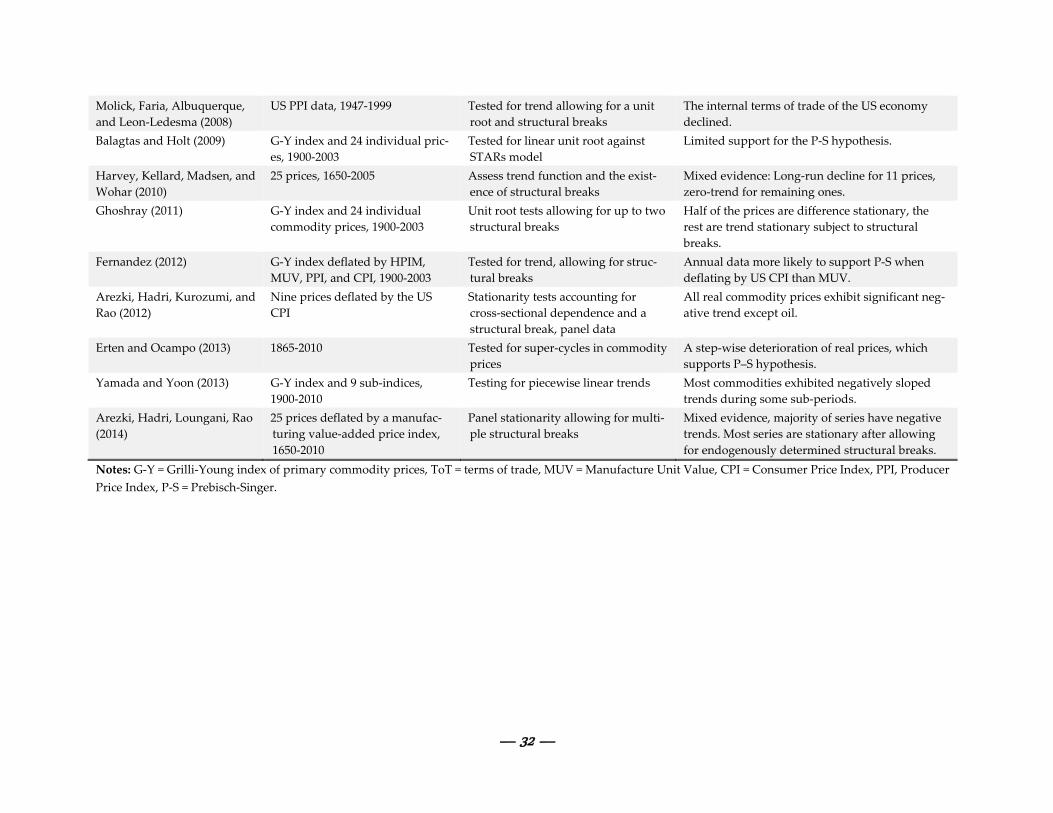
— 32 —

Molick, Faria, Albuquerque,

and Leon-Ledesma (2008)

US PPI data, 1947-1999 Tested for trend allowing for a unit

root and structural breaks

The internal terms of trade of the US economy

declined.

Balagtas and Holt (2009) G-Y index and 24 individual pric-

es, 1900-2003

Tested for linear unit root against

STARs model

Limited support for the P-S hypothesis.

Harvey, Kellard, Madsen, and

Wohar (2010)

25 prices, 1650-2005 Assess trend function and the exist-

ence of structural breaks

Mixed evidence: Long-run decline for 11 prices,

zero-trend for remaining ones.

Ghoshray (2011) G-Y index and 24 individual

commodity prices, 1900-2003

Unit root tests allowing for up to two

structural breaks

Half of the prices are difference stationary, the

rest are trend stationary subject to structural

breaks.

Fernandez (2012) G-Y index deflated by HPIM,

MUV, PPI, and CPI, 1900-2003

Tested for trend, allowing for struc-

tural breaks

Annual data more likely to support P-S when

deflating by US CPI than MUV.

Arezki, Hadri, Kurozumi, and

Rao (2012)

Nine prices deflated by the US

CPI

Stationarity tests accounting for

cross-sectional dependence and a

structural break, panel data

All real commodity prices exhibit significant neg-

ative trend except oil.

Erten and Ocampo (2013) 1865-2010 Tested for super-cycles in commodity

prices

A step-wise deterioration of real prices, which

supports P–S hypothesis.

Yamada and Yoon (2013) G-Y index and 9 sub-indices,

1900-2010

Testing for piecewise linear trends Most commodities exhibited negatively sloped

trends during some sub-periods.

Arezki, Hadri, Loungani, Rao

(2014)

25 prices deflated by a manufac-

turing value-added price index,

1650-2010

Panel stationarity allowing for multi-

ple structural breaks

Mixed evidence, majority of series have negative

trends. Most series are stationary after allowing

for endogenously determined structural breaks.

Notes: G-Y = Grilli-Young index of primary commodity prices, ToT = terms of trade, MUV = Manufacture Unit Value, CPI = Consumer Price Index, PPI, Producer

Price Index, P-S = Prebisch-Singer.

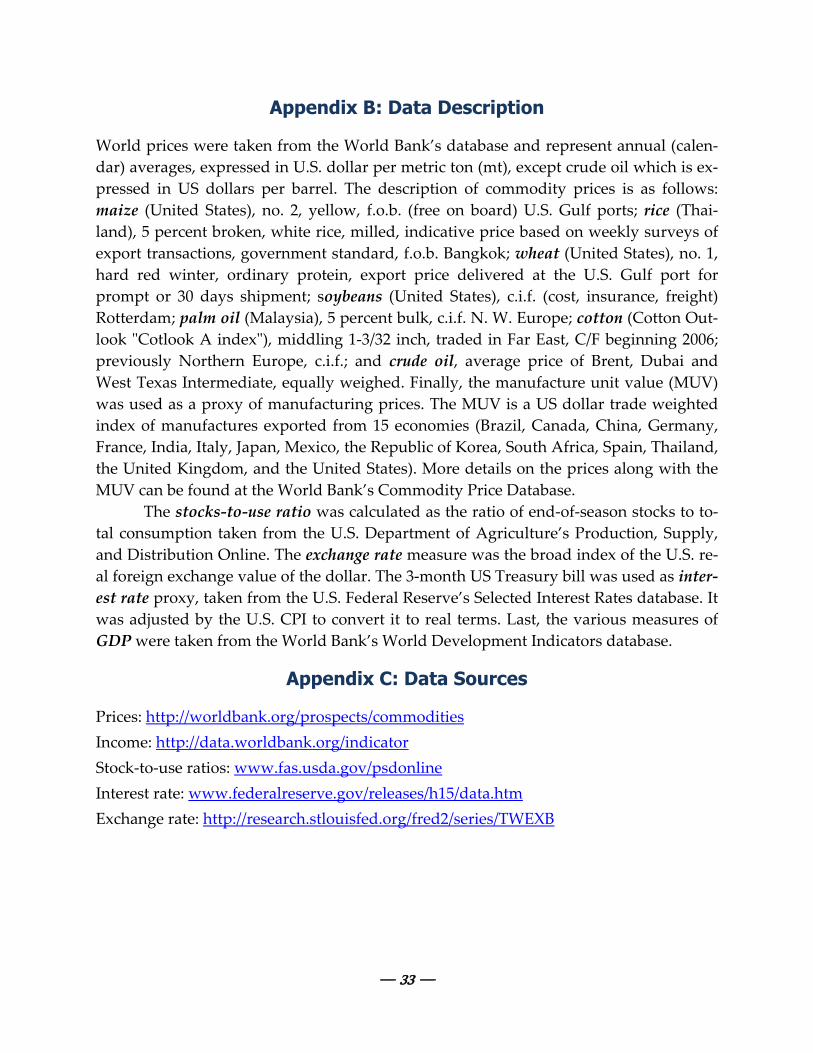
— 33 —

Appendix B: Data Description

World prices were taken from the World Bank’s database and represent annual (calen-

dar) averages, expressed in U.S. dollar per metric ton (mt), except crude oil which is ex-

pressed in US dollars per barrel. The description of commodity prices is as follows:

maize (United States), no. 2, yellow, f.o.b. (free on board) U.S. Gulf ports; rice (Thai-

land), 5 percent broken, white rice, milled, indicative price based on weekly surveys of

export transactions, government standard, f.o.b. Bangkok; wheat (United States), no. 1,

hard red winter, ordinary protein, export price delivered at the U.S. Gulf port for

prompt or 30 days shipment; soybeans (United States), c.i.f. (cost, insurance, freight)

Rotterdam; palm oil (Malaysia), 5 percent bulk, c.i.f. N. W. Europe; cotton (Cotton Out-

look "Cotlook A index"), middling 1-3/32 inch, traded in Far East, C/F beginning 2006;

previously Northern Europe, c.i.f.; and crude oil, average price of Brent, Dubai and

West Texas Intermediate, equally weighed. Finally, the manufacture unit value (MUV)

was used as a proxy of manufacturing prices. The MUV is a US dollar trade weighted

index of manufactures exported from 15 economies (Brazil, Canada, China, Germany,

France, India, Italy, Japan, Mexico, the Republic of Korea, South Africa, Spain, Thailand,

the United Kingdom, and the United States). More details on the prices along with the

MUV can be found at the World Bank’s Commodity Price Database.

The stocks-to-use ratio was calculated as the ratio of end-of-season stocks to to-

tal consumption taken from the U.S. Department of Agriculture’s Production, Supply,

and Distribution Online. The exchange rate measure was the broad index of the U.S. re-

al foreign exchange value of the dollar. The 3-month US Treasury bill was used as inter-

est rate proxy, taken from the U.S. Federal Reserve’s Selected Interest Rates database. It

was adjusted by the U.S. CPI to convert it to real terms. Last, the various measures of

GDP were taken from the World Bank’s World Development Indicators database.

Appendix C: Data Sources

Prices: http://worldbank.org/prospects/commodities

Income: http://data.worldbank.org/indicator

Stock-to-use ratios: www.fas.usda.gov/psdonline

Interest rate: www.federalreserve.gov/releases/h15/data.htm

Exchange rate: http://research.stlouisfed.org/fred2/series/TWEXB