Embed Size (px)
Citation preview
Reconfigurable Modular Mobile Robotic Platform
A Major Qualifying Project Report Submitted to the Faculty
of the
WORCESTER POLYTECHNIC INSTITUTE In partial fulfillment of the requirements for the
Degree of Bachelor of Science in Robotics Engineering
on 3/16/10
by
_______________________ _______________________ _______________________
Matt Bienia [email protected]
Dan Garcia [email protected]
Karl Wajcs [email protected]
Approved:
_______________________
TaskinPadir
Project Number: RBE-TP1-RMP1

ii
Acknowledgements We would like to thank several people for their help throughout the duration of this project,
without which this would not have been possible.
Atmel Corp. and The Fastener Source for their generous donation of electrical and mechanical components, respectively.
The Washburn Shops Faculty for the use of their time and resources.
Mike Niziol of MG Machine Co. for his generous donation of facilities and material for CNC machining.
Chip Bienia for his experience, time, and resources involving CNC manufacturing.
Ivo Dobrev for his knowledge and support in the development of robot kinematics.
Sam Kaplan and Kevin O’Brien for their dedicated work on the balance algorithm.
Professor Hugh Lauer for his expertise and instruction in distributed processing and data structures.
Professor Joseph Beck for his expertise and instruction in artificial intelligence.
And finally, Professor Taşkin Padir for continued support, ideas, and patience throughout the ups and downs that were encountered during this project.

iii
Abstract This project addresses the inflexibility of modern robotics by developing a modular robotic
platform, capable of using various modules that can be added and removed to a base unit in a short
amount of time. The scope of the project limited development of modules to a 3-DOF leg. The proof of
concept was established by developing a main communications board capable of detecting attached
peripherals, and individual leg circuit boards capable of full PID control utilizing inverse kinematics to
precisely place the end of the leg. Mechanical issues prevented the leg constructed from being fully
functional, however plans have been developed to address all issues found in the development of this
platform.
iv
Table of Contents Acknowledgements............................................................................................................................ ii
Abstract ............................................................................................................................................ iii
Table of Contents .............................................................................................................................. iv
Table of Figures: ............................................................................................................................... vi
List of Tables: ................................................................................................................................... vii
Table of Equations .......................................................................................................................... viii
Table of Code Samples .................................................................................................................... viii
Authorship........................................................................................................................................ ix
1. Introduction ...............................................................................................................................1
1.1. Background .................................................................................................................................. 2
1.2. Report Organization .................................................................................................................... 5
2. Methodology ..............................................................................................................................6
2.1. Design Specifications ................................................................................................................... 6
2.2. Robot Design: Mechanical ........................................................................................................... 7
2.2.1. Leg Design ............................................................................................................................... 8
2.2.2. Gearbox ................................................................................................................................... 9
2.2.3. Hip Joint Design ..................................................................................................................... 12
2.2.4. Static Force Analysis .............................................................................................................. 13
2.2.5. Chassis Design ....................................................................................................................... 15
2.3. Robot Design: Electrical System ................................................................................................ 16
2.3.1. Control System and Distributed Processing Overview .......................................................... 16
2.3.2. Leg Control Unit (LCU) Hardware .......................................................................................... 17
2.3.3. Main Communications Board (MCB) Hardware .................................................................... 23
2.3.4. Main Processing Unit (MPU) Hardware ................................................................................ 26
2.3.5. Miscellaneous Electrical Considerations ............................................................................... 28
2.4. Robot Design: Software and Control Systems ........................................................................... 28
2.4.1. Communications Protocol ..................................................................................................... 28
2.4.2. MPU Software & Operational Characteristics ....................................................................... 37
2.4.3. LCU Software & Operational Characteristics ........................................................................ 45
2.4.4. Software Model Diagrams ..................................................................................................... 58
3. Results ..................................................................................................................................... 63
v
3.1. Mechanical Design Revisions ..................................................................................................... 64
3.1.1. Review of the Initial Design ................................................................................................... 65
3.1.2. Goals of the Revised Design .................................................................................................. 66
3.2. Electrical System Observations.................................................................................................. 74
3.2.1. LCU PCB Construction and Issues .......................................................................................... 74
3.2.2. MCB PCB Construction and Issues ........................................................................................ 75
3.3. Software Timing and Effective Control Frequencies ................................................................. 76
3.3.1. PID Loop Timing .................................................................................................................... 77
3.3.2. Total Leg PID Loop Timing ..................................................................................................... 77
3.3.3. Inverse Kinematics Timing..................................................................................................... 78
3.3.4. Forward Kinematics Timing ................................................................................................... 79
3.3.5. Total LCU Command Process Timing ..................................................................................... 79
3.4. Budget ....................................................................................................................................... 80
3.4.1. Mechanical Budget ................................................................................................................ 80
3.4.2. Electrical Budget .................................................................................................................... 82
4. Future Work ............................................................................................................................. 84
5. Conclusion ................................................................................................................................ 85
6. References ............................................................................................................................... 86
7. Appendices............................................................................................................................... 89
7.1. LCU Schematics .......................................................................................................................... 89
7.2. MCB Schematics ........................................................................................................................ 96
7.3. MPU Schematics ...................................................................................................................... 104
vi
Table of Figures: Figure 1: Kamimura Experimental Module (1) .............................................................................................. 2Figure 2: Demonstration of Structural Disassembly and Reconstruction (3) ............................................... 3Figure 3: BigDog Robot (4) ............................................................................................................................ 4Figure 4: Conceptual ReMMRP Illustration ................................................................................................... 7Figure 5: Conceptual Leg Illustration ............................................................................................................ 8Figure 6: Conceptual Worm Gearbox Illustration ....................................................................................... 10Figure 7: Conceptual Miter Gearbox Illustration ........................................................................................ 10Figure 8: Miter Gearbox Design .................................................................................................................. 12Figure 9: Internal View of the Gearbox ....................................................................................................... 12Figure 10: Hip Joint Design .......................................................................................................................... 13Figure 11: Static Force Calculation Figure. .................................................................................................. 14Figure 12: The Robot Chassis ...................................................................................................................... 16Figure 13: Labeled Top View of the LCU ..................................................................................................... 17Figure 14: Front and Back View of a Blank LCU PCB ................................................................................... 22Figure 15: Labeled Top View of the MCB .................................................................................................... 23Figure 16: Front and Back Views of a Blank MCB PCB ................................................................................ 26Figure 17: Labeled Top View of the MPU ................................................................................................... 27Figure 18: Front and Back Views of a Blank MPU PCB ................................................................................ 28Figure 19: Single Master / Single Slave Configuration ................................................................................ 30Figure 20: Single Master / Multiple Slave Configuration ............................................................................ 30Figure 21: Master / Slave Data Transfer ..................................................................................................... 31Figure 22: SPI Initial Single Byte Data Exchange ......................................................................................... 33Figure 23: SPI Indexed Byte Transfer .......................................................................................................... 33Figure 24: Robot Coordinate Frame & Port Numbering ............................................................................. 39Figure 25: Base of Support and Robot Chassis Centroids ........................................................................... 42Figure 26: The Stabilizing Vector ................................................................................................................. 43Figure 27: Z-Constrained Leg Workspace ................................................................................................... 43Figure 28: Leg Joint Coordinate Frames ...................................................................................................... 46Figure 29: PWM vs Analog Drive ................................................................................................................. 53Figure 30: Conceptual H-Bridge Diagram .................................................................................................... 54Figure 31: Forward and Reverse Configurations of the Conceptual H-Bridge ............................................ 55Figure 32: PID Control Process Diagram ..................................................................................................... 57Figure 33: MPU Software Flow Diagram .................................................................................................... 59Figure 34: LCU Software Flow Diagram ...................................................................................................... 60Figure 35: Integrated Software Control Flow Diagram ............................................................................... 62Figure 36: Completed Robot (1 Leg) ........................................................................................................... 64Figure 37: Conceptual Illustration of Revised ReMMRP Design ................................................................. 65Figure 38: Side View Comparison of the previous gearbox (Top) and the new gearbox (Bottom) ............ 67Figure 39: Top view comparison of the previous gearbox (Left) and the new gearbox (Right) ................. 67
vii
Figure 40: Comparison between the old Thigh Plate (Top) and the new Leg Plate (Bottom) .................... 68Figure 41: Comparison View of the old HMA (Left) compared to the new design (Right) ........................ 69Figure 42: Comparison View of the Current HCB (Left) and the Revised Design (Right). ........................... 70Figure 43: Static Force Calculation for the Revised Design ......................................................................... 70Figure 44: Revised Chassis Short Plate CosmosXpress Results ................................................................... 72Figure 45: Displacement of the Revised Short Chassis Plate ...................................................................... 73Figure 46: Chassis Long Plate CosmosXpress Results ................................................................................. 73Figure 47: Resulting Displacement of the Long Chassis Plate ..................................................................... 74Figure 48: Assembled LCU Board ................................................................................................................ 75Figure 49: Assembled MCB Board ............................................................................................................... 76Figure 50: Single PID Loop timing ............................................................................................................... 77Figure 51: Total PID Loop Timing ............................................................................................................... 77Figure 52: Inverse Kinematics Loop Timing ................................................................................................ 78Figure 53: Forward Kinematics Loop Timing ............................................................................................... 79Figure 54: Complete LCU Leg Motion Command Timing ............................................................................ 79
List of Tables: Table 1: Gearbox Trade Study ..................................................................................................................... 11Table 2: Joint Motor Spec Comparison and Trade Study ............................................................................ 19Table 3: Graphic Comparison of LCU Connectors (11)(12)(13)(14)(15)(16) ............................................... 21Table 4: Comparison of ATMega164/324/644P Communication Modes ................................................... 29Table 5: Denavit-Hartenberg Parameters for ReMMRP Leg Modules ........................................................ 47Table 6: Ziegler-Nichols Ultimate Gain Equations ...................................................................................... 57Table 7: Design Specification Compliance .................................................................................................. 63Table 8: Comparison of Current and Revised Motor Torques .................................................................... 71Table 9: Mechanical Budget per Leg ........................................................................................................... 81Table 10: Single Purchase Material Budget ................................................................................................ 82Table 11: LCU Itemized budget ................................................................................................................... 83Table 12: MCB Itemized Budget .................................................................................................................. 83Table 13: MPU Itemized Budget ................................................................................................................. 84
viii
Table of Equations Equation 1: Motor 3 Torque ....................................................................................................................... 14Equation 2: Motor 2 Torque ....................................................................................................................... 14Equation 3: Motor 1 Torque ....................................................................................................................... 15Equation 4: Minimum Joint 2 Angle for Horizontal Movement .................................................................. 15Equation 5: Choose Function ...................................................................................................................... 41Equation 6: Total Possible Leg Configurations of ReMMRP ....................................................................... 41Equation 7: Area of a Polygon ..................................................................................................................... 42Equation 8: Polygon Centroid Equations (7) ............................................................................................... 42Equation 9: Denavit-Hartenberg Homogeneous Transformation .............................................................. 46Equation 10: Parameterized Sequential Homogenous Transformation Matrices ...................................... 47Equation 11: Homogeneous Transformation from Coordinate Frame 0 to Coordinate Frame 3 .............. 47Equation 12: Transformation from Leg Coordinate Frame to Robot Coordinate Frame ........................... 48Equation 13: Angular Position of the Horizontal Hip Joint ......................................................................... 50Equation 14: Angular Position of the Vertical Hip Joint .............................................................................. 51Equation 15: Angular Position of the Knee Joint ........................................................................................ 51Equation 16: Linear Interpolation ............................................................................................................... 55Equation 17: Motor 3 Torque in Revised Leg .............................................................................................. 71Equation 18: Motor 2 Torque in Revised Leg .............................................................................................. 71Equation 19: Motor 1 Torque in Revised Leg .............................................................................................. 71
Table of Code Samples Code Sample 1: Slave SBDE Communication Routine ................................................................................ 36Code Sample 2: Master SBDE Communication Routine ............................................................................. 37Code Sample 3: Forward Kinematics .......................................................................................................... 50Code Sample 4: Inverse Kinematics ............................................................................................................ 52Code Sample 5: PID Control ........................................................................................................................ 58
ix
Authorship Introduction……………………………………………………………………………………………………………….. All
Background………………………………………………………………………………………………………………… KW
Methodology
Robot Design: Mechanical………………………………………………………………………………. KW
Robot Design: Electrical System ……………………………………………………………………… MB
Robot Design: Software and Control Systems…………………………………………………. DG
Results
Mechanical Design Revisions………………………………………………………………………….. KW
Electrical System Observation………………………………………………………………………….. MB
Software Timing and Effective Control Frequencies………………………………………….. DG
Budget………………………………………………………………………………………………………………. MB & KW
Future Work……………………………………………………………………………………………………………….. MB & KW
Conclusion………………………………………………………………………………………………………………….. All
1
1. Introduction The development and control of (self-)reconfigurable and modular robotic platforms have
emerged as a new research area in robotics within the past two decades. The field addresses new
challenges that come with the design, modeling, implementation and control of autonomous robots
whose kinematic structures can vary over time depending on the physical environment that they are in.
The reconfigurable modular robots have two important features which make them desirable in
applications; flexibility and robustness. They can adapt their shape and form with respect to changes in
their environments and they can accommodate failures within modules provided that they possess
redundancy.
A limitation to the field of robotics is that robots are designed to accomplish a specific task; this
limits the versatility of these machines. The development of a modular robotics platform, specifically
intended for rapid prototyping of autonomous systems, would promote the marketing of more products
as well as the creation of more jobs in the assembly and testing of various configurations of the
platform. Creation of various specialized units from a base of modular components would also allow
any of these units to be quickly and easily repaired or reconfigured in the field.
The goal of this project is to design, construct, and demonstrate a reconfigurable mobile
platform that addresses, at least in part, the issues outlined above. The project outcome will be a proof
of concept for future development and commercialization of a reconfigurable mobile robot.
Within the scope of this project, the terms “reconfigurable,” “mobile,” and “modular” are
defined as follows:
A reconfigurable robot is one that is capable of attaining various configurations by the addition
or removal of peripheral attachments (leg, arm, sensor, etc.) to predefined connection points
existing on the robot chassis.
A mobile robot is one that is capable of autonomous or controlled locomotion to change its
relative position and orientation with respect to a global coordinate frame.
A modular robot is one that is built using a variety of peripheral units employing standardized
electrical and mechanical connections and communications.
2
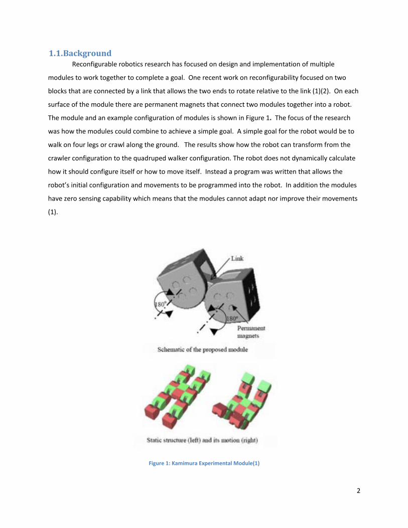
1.1. Background Reconfigurable robotics research has focused on design and implementation of multiple
modules to work together to complete a goal. One recent work on reconfigurability focused on two
blocks that are connected by a link that allows the two ends to rotate relative to the link (1)(2). On each
surface of the module there are permanent magnets that connect two modules together into a robot.
The module and an example configuration of modules is shown in Figure 1. The focus of the research
was how the modules could combine to achieve a simple goal. A simple goal for the robot would be to
walk on four legs or crawl along the ground. The results show how the robot can transform from the
crawler configuration to the quadruped walker configuration. The robot does not dynamically calculate
how it should configure itself or how to move itself. Instead a program was written that allows the
robot’s initial configuration and movements to be programmed into the robot. In addition the modules
have zero sensing capability which means that the modules cannot adapt nor improve their movements
(1).
Figure 1: Kamimura Experimental Module(1)
3
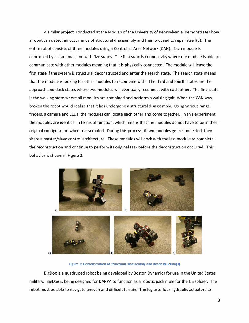
A similar project, conducted at the Modlab of the University of Pennsylvania, demonstrates how
a robot can detect an occurrence of structural disassembly and then proceed to repair itself(3). The
entire robot consists of three modules using a Controller Area Network (CAN). Each module is
controlled by a state machine with five states. The first state is connectivity where the module is able to
communicate with other modules meaning that it is physically connected. The module will leave the
first state if the system is structural deconstructed and enter the search state. The search state means
that the module is looking for other modules to recombine with. The third and fourth states are the
approach and dock states where two modules will eventually reconnect with each other. The final state
is the walking state where all modules are combined and perform a walking gait. When the CAN was
broken the robot would realize that it has undergone a structural disassembly. Using various range
finders, a camera and LEDs, the modules can locate each other and come together. In this experiment
the modules are identical in terms of function, which means that the modules do not have to be in their
original configuration when reassembled. During this process, if two modules get reconnected, they
share a master/slave control architecture. These modules will dock with the last module to complete
the reconstruction and continue to perform its original task before the deconstruction occurred. This
behavior is shown in Figure 2.
Figure 2: Demonstration of Structural Disassembly and Reconstruction(3)
BigDog is a quadruped robot being developed by Boston Dynamics for use in the United States
military. BigDog is being designed for DARPA to function as a robotic pack mule for the US soldier. The
robot must be able to navigate uneven and difficult terrain. The leg uses four hydraulic actuators to

4
control the position and movement. BigDog must be able to determine how it is interacting with its
environment, how it is positioned in space and how to position its legs to achieve balance and the
desired gait.
BigDog uses kinematics and the ground reaction forces generated by the robot as the basis for
its control systems. BigDog uses 50 sensors to measure leg positions, accelerations and the various
forces exerted and experienced by the robot. BigDog has different algorithms to handle different types
of terrain like mud, snow or sand as well as handling different inclines. The robot must be able to uses
its sensors to determine which type of algorithm to use and how to apply it. Although BigDog is
controlled by a human, this is only used to give it a direction and speed of travel, all calculations for leg
placement and balance is handled by the robot.
Figure 3: BigDog Robot(4)
The aforementioned robotic systems demonstrate reconfigurability, modularity, and mobility
and illustrate the benefits of each idea as it applies to the advancing frontier of the robotics industry.
The Reconfigurable Modular Mobile Robotics Platform (ReMMRP) takes the next logical step in
innovation and combines these concepts into a robust, adaptive, plug-and-play robotic system. This
report details the development of this platform and the integration of the mechanical, electrical, and
software subsystems that make up the ReMMRP.
5
1.2. Report Organization This report is broken down into the following sections:
Methodology, separated into the following components: o mechanical o electrical o software
Results Future Work Conclusions
6
2. Methodology The ReMMRP explores the integration of the concepts of reconfigurability, modularity, and
mobility in a single robotic platform. In order to achieve this goal, the robot must be able to accept
peripheral leg modules, recognize their presence and location, and coordinate their actions. The
ReMMRP must have:
a base unit, or chassis, that serves as a common connection hub for all peripheral modules.
leg modules capable of supporting the robot chassis and allowing mobility in three dimensions.
the ability to detect addition or removal of peripheral modules in real time.
the ability to control peripheral modules in real time.
the ability to determine if the present configuration is balanceable, and if so balance.
2.1. Design Specifications In order to meet the requirements outlined in Section 2, specifications for the mechanical,
electrical, and software systems of the leg modules and chassis must be as follows:
Chassis:
o The chassis will have 12 connection points – 2 on each short side, 4 on each long side.
o The chassis must contain a centralized power distribution and communications hub.
o The chassis must contain a processor responsible for coordinating the actions of all
peripheral modules, referred to as the Main Processing Unit (MPU).
o The MPU must be interchangeable.
o MPU software must determine actions for all peripheral modules and delegate
commands to them in real time.
o The chassis must have a dedicated processor responsible for detecting the addition or
removal of peripheral modules in real time independently of the MPUs operation,
referred to as the STATUS processor.
o STATUS processor software must operate in real time, allowing MPU to have immediate
knowledge of attached peripherals at any given time.
Leg Modules:
o The legs modules will have 3 degrees of freedom (DOF)
o The leg must operate in 3-dimensional space.
7
o The leg must have position sensors integrated into each joint.
o The joint motors must be mounted internally in each leg link.
o Each leg module must have self-contained control system, referred to as a Leg Control
Unit (LCU).
o The LCU must have a processor capable of handling the software controls.
o The LCU must distribute power to joint motors and read joint position sensors.
o The LCU must be able to relay signals to the main control system.
o LCU software must respond to commands from MPU with higher priority than any other
task inherent to LCU software.
o Communications protocol must exist for data transfer among the MPU, STATUS
processor, and LCUs).
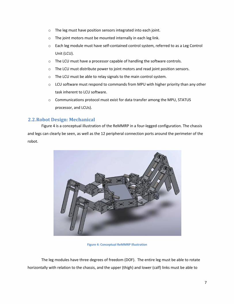
2.2. Robot Design: Mechanical Figure 4 is a conceptual illustration of the ReMMRP in a four-legged configuration. The chassis
and legs can clearly be seen, as well as the 12 peripheral connection ports around the perimeter of the
robot.
Figure 4: Conceptual ReMMRP Illustration
The leg modules have three degrees of freedom (DOF). The entire leg must be able to rotate
horizontally with relation to the chassis, and the upper (thigh) and lower (calf) links must be able to
8
rotate vertically with relation to the chassis. The robot must be able to determine each link’s position,
therefore the leg must have sensors integrated into the design. The chassis will have 12 connection
points around its perimeter. There will be two ports on each short side, and four on each long side. The
long side of the chassis will be twice the length of the short side.
In order to provide the legs the greatest movement possible and to reduce collisions, the joint
motors must be mounted internally in each leg link. However to achieve this specification, the motors
will be perpendicular to the axis of rotation. In order to transfer the motor’s rotation to the leg joint a
gearbox is necessary.
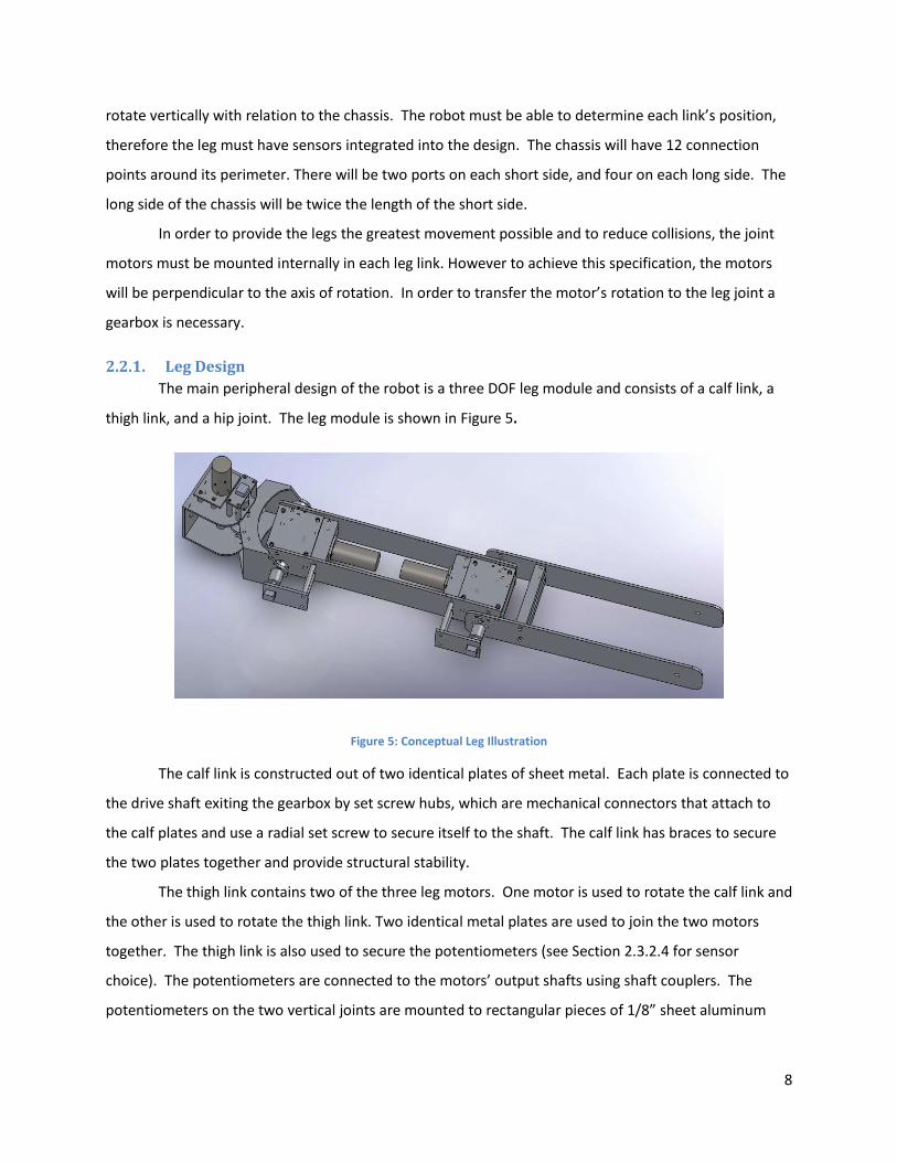
2.2.1. Leg Design The main peripheral design of the robot is a three DOF leg module and consists of a calf link, a
thigh link, and a hip joint. The leg module is shown in Figure 5.
Figure 5: Conceptual Leg Illustration
The calf link is constructed out of two identical plates of sheet metal. Each plate is connected to
the drive shaft exiting the gearbox by set screw hubs, which are mechanical connectors that attach to
the calf plates and use a radial set screw to secure itself to the shaft. The calf link has braces to secure
the two plates together and provide structural stability.
The thigh link contains two of the three leg motors. One motor is used to rotate the calf link and
the other is used to rotate the thigh link. Two identical metal plates are used to join the two motors
together. The thigh link is also used to secure the potentiometers (see Section 2.3.2.4 for sensor
choice). The potentiometers are connected to the motors’ output shafts using shaft couplers. The
potentiometers on the two vertical joints are mounted to rectangular pieces of 1/8” sheet aluminum
9
which are secured to the thigh link by two #6-32 screws which use spacers to set the potentiometer at
the correct distance from the thigh link.
The hip joint of the leg module is constructed from two machined pieces of aluminum tube
stock. One piece is connected to the robot chassis and has the port connector. This piece allows for the
horizontal rotation of the leg. The other piece connects the thigh link to the hip joint. This piece allows
for the vertical rotation of the leg from the hip.
2.2.2. Gearbox Commercial gearboxes fall into two distinct categories. The first are those designed for
industrial applications, and the second are those designed for robotic hobbyists. The industrial
gearboxes are typically large, weigh several pounds, and are designed for higher torque applications
than required by the ReMMRP. The hobbyist gearboxes are designed for simple robots and made of
cheap plastic. The gearboxes would break under the loads of this robot and are therefore unsuitable. As
a result, ReMMRP uses a custom gearbox. Due to the fact that the gearboxes are a custom design, the
leg will be designed around this gearbox. There are two types of gears that can be used for the gearbox:
a worm gear and a miter gear. Each gear type has advantages and disadvantages as will be discussed
below.
2.2.2.1. Worm Gearbox The first gearbox design considered for the project is a worm gear system. The primary reason
for the use of the worm gears is to make the legs non-backdriveable. The non-backdriveability would
require less power to be consumed by the motors as the motors would not have to constantly be
correcting the leg position of the robot. Worm gears typically have a high gear ratio, meaning that a
weaker motor could be chosen when compared to a gear train with little or no gearing down.
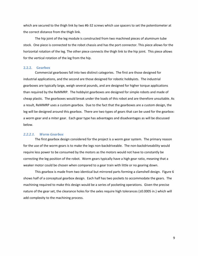
This gearbox is made from two identical but mirrored parts forming a clamshell design. Figure 6
shows half of a conceptual gearbox design. Each half has two pockets to accommodate the gears. The
machining required to make this design would be a series of pocketing operations. Given the precise
nature of the gear set, the clearance holes for the axles require high tolerances (±0.0005 in.) which will
add complexity to the machining process.
10
Figure 6: Conceptual Worm Gearbox Illustration
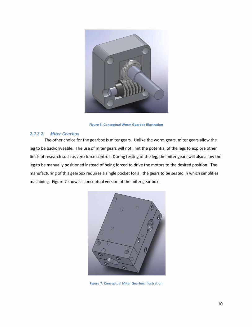
2.2.2.2. Miter Gearbox The other choice for the gearbox is miter gears. Unlike the worm gears, miter gears allow the
leg to be backdriveable. The use of miter gears will not limit the potential of the legs to explore other
fields of research such as zero force control. During testing of the leg, the miter gears will also allow the
leg to be manually positioned instead of being forced to drive the motors to the desired position. The
manufacturing of this gearbox requires a single pocket for all the gears to be seated in which simplifies
machining. Figure 7 shows a conceptual version of the miter gear box.
Figure 7: Conceptual Miter Gearbox Illustration
11
2.2.2.3. Gearbox Selection In order to select the best type of gear for the design a trade study is conducted as shown in
Table 1. The trade study has three categories for each gearbox type to be rated on. The categories are
cost, torque and ease of manufacturing. Each of these categories is given a weight of 1-5 based on their
importance. The two gearbox types are then given a rating on each category. The rating and the weight
are multiplied together for the final score. These scores are then added together.
Worm Gearbox Miter Gearbox
Cost (2) 2 * 2 = 4 3 * 2 = 6
Torque (3) 4 * 3 = 12 3 * 3 = 9
Manufacturability (4) 2 * 4 = 8 3 * 4 = 12
Total 24 27
Table 1: Gearbox Trade Study
According to the trade study, the miter gear is the better gear choice for the gearbox. Both
types of gears are close in price. The worm gear can have high gear ratio, but miter gears can also
increase their torque output with a modified gear ratio. Manufacturing a miter gear box is also easier to
do. Therefore, the miter gearbox will be used to construct the leg modules.
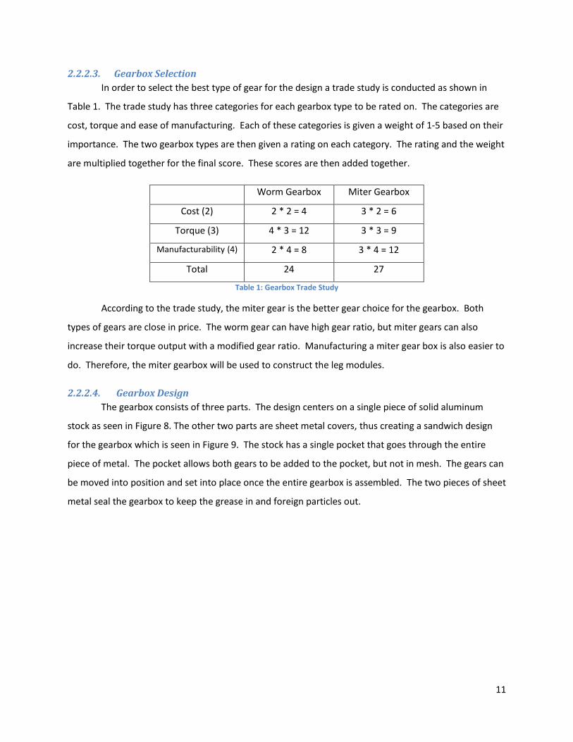
2.2.2.4. Gearbox Design The gearbox consists of three parts. The design centers on a single piece of solid aluminum
stock as seen in Figure 8. The other two parts are sheet metal covers, thus creating a sandwich design
for the gearbox which is seen in Figure 9. The stock has a single pocket that goes through the entire
piece of metal. The pocket allows both gears to be added to the pocket, but not in mesh. The gears can
be moved into position and set into place once the entire gearbox is assembled. The two pieces of sheet
metal seal the gearbox to keep the grease in and foreign particles out.
12
Figure 8: Miter Gearbox Design
Figure 9: Internal View of the Gearbox
This gearbox has several advantages. The screw pattern on the top and bottom face of the
gearbox gas only 4 screws for easy attachment of cover plates. The sizes of the screws are standardized
to a single size of 6-32, which minimizes the number of different tools necessary to machine and
assemble the part. The pocket of the gearbox also relies on looser tolerances. Often end-mill cutters will
undercut the pocket which has the potential of forcing the gears out of their meshed position. By
increasing the dimensions of the pocket it reduces the impact undercutting will have and decrease
machining time. The gearbox design utilizes press fit ball bearings for easy manufacturing and assembly.
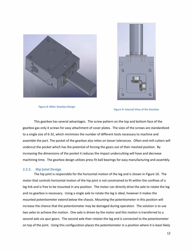
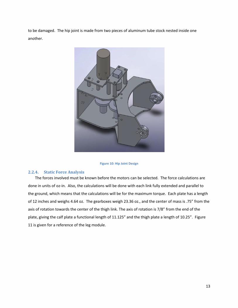
2.2.3. Hip Joint Design The hip joint is responsible for the horizontal motion of the leg and is shown in Figure 10. The
motor that controls horizontal motion of the hip joint is not constrained to fit within the confines of a
leg link and is free to be mounted in any position. The motor can directly drive the axle to rotate the leg
and no gearbox is necessary. Using a single axle to rotate the leg is ideal, however it makes the
mounted potentiometer extend below the chassis. Mounting the potentiometer in this position will
increase the chance that the potentiometer may be damaged during operation. The solution is to use
two axles to achieve the motion. One axle is driven by the motor and this motion is transferred to a
second axle via spur gears. The second axle then rotates the leg and is connected to the potentiometer
on top of the joint. Using this configuration places the potentiometer in a position where it is least likely
13
to be damaged. The hip joint is made from two pieces of aluminum tube stock nested inside one
another.
Figure 10: Hip Joint Design
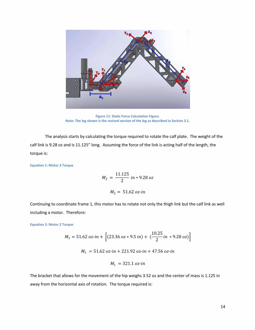
2.2.4. Static Force Analysis The forces involved must be known before the motors can be selected. The force calculations are
done in units of oz-in. Also, the calculations will be done with each link fully extended and parallel to
the ground, which means that the calculations will be for the maximum torque. Each plate has a length
of 12 inches and weighs 4.64 oz. The gearboxes weigh 23.36 oz., and the center of mass is .75” from the
axis of rotation towards the center of the thigh link. The axis of rotation is 7/8” from the end of the
plate, giving the calf plate a functional length of 11.125” and the thigh plate a length of 10.25”. Figure
11 is given for a reference of the leg module.
14
Figure 11: Static Force Calculation Figure. Note: The leg shown is the revised version of the leg as described in Section 3.1.
The analysis starts by calculating the torque required to rotate the calf plate. The weight of the
calf link is 9.28 oz and is 11.125” long. Assuming the force of the link is acting half of the length, the
torque is:
Equation 1: Motor 3 Torque
𝑀𝑀2 = 11.125
2 𝑖𝑖𝑖𝑖 ∗ 9.28 𝑜𝑜𝑜𝑜
𝑀𝑀2 = 51.62 𝑜𝑜𝑜𝑜-𝑖𝑖𝑖𝑖
Continuing to coordinate frame 1, this motor has to rotate not only the thigh link but the calf link as well
including a motor. Therefore:
Equation 2: Motor 2 Torque
𝑀𝑀1 = 51.62 𝑜𝑜𝑜𝑜-𝑖𝑖𝑖𝑖 + �(23.36 𝑜𝑜𝑜𝑜 ∗ 9.5 𝑖𝑖𝑖𝑖) + (10.25
2𝑖𝑖𝑖𝑖 ∗ 9.28 𝑜𝑜𝑜𝑜)�
𝑀𝑀1 = 51.62 𝑜𝑜𝑜𝑜-𝑖𝑖𝑖𝑖 + 221.92 𝑜𝑜𝑜𝑜-𝑖𝑖𝑖𝑖 + 47.56 𝑜𝑜𝑜𝑜-𝑖𝑖𝑖𝑖
𝑀𝑀1 = 321.1 𝑜𝑜𝑜𝑜-𝑖𝑖𝑖𝑖
The bracket that allows for the movement of the hip weighs 3.52 oz and the center of mass is 1.125 in
away from the horizontal axis of rotation. The torque required is:
15
Equation 3: Motor 1 Torque
𝑀𝑀0 = 321.1 𝑜𝑜𝑜𝑜-𝑖𝑖𝑖𝑖 + [(3.125 𝑖𝑖𝑖𝑖 ∗ 23.36 𝑜𝑜𝑜𝑜) + (1.125 𝑖𝑖𝑖𝑖 ∗ 3.52 𝑜𝑜𝑜𝑜)]
𝑀𝑀0 = 321.1 𝑜𝑜𝑜𝑜-𝑖𝑖𝑖𝑖 + 73 𝑜𝑜𝑜𝑜-𝑖𝑖𝑖𝑖 + 3.96 𝑜𝑜𝑜𝑜-𝑖𝑖𝑖𝑖
𝑀𝑀0 = 398.06 𝑜𝑜𝑜𝑜-𝑖𝑖𝑖𝑖
Based on the calculations performed, the Lynxmotion PGHM-04 is used. The motor selection is
discussed in detail in Section 2.3.2.2. The motor is rated at 341.76 oz-in of torque and weighs 3.59 oz.
Although this torque is below the maximum calculated torque for the thigh link, the specifications state
that the leg does not have to be able to rotate the leg at maximum torque.
In order for the entire leg to be rotated the thigh and calf links must be at some angle with
respect to the horizontal axis. Assuming that the calf and the thigh links are in line with each other and
the motor is 85% efficient, which gives the motor a torque rating of 289.85 oz-in. The angle required is
as follows:
Equation 4: Minimum Joint 2 Angle for Horizontal Movement
289.85 𝑜𝑜𝑜𝑜-𝑖𝑖𝑖𝑖 = 3.96 𝑜𝑜𝑜𝑜-𝑖𝑖𝑖𝑖 + (394.1 𝑜𝑜𝑜𝑜-𝑖𝑖𝑖𝑖 ∗ cos𝜃𝜃)
285.89 𝑜𝑜𝑜𝑜-𝑖𝑖𝑖𝑖 = 394.1 𝑜𝑜𝑜𝑜-𝑖𝑖𝑖𝑖 ∗ cos𝜃𝜃
285.89394.1
= cos𝜃𝜃
cos𝜃𝜃 = .725
𝜃𝜃 = 43.5
2.2.5. Chassis Design The chassis, shown in Figure 12, is made up of four plates of aluminum connected by four angle
brackets. There are two short sides containing two ports each and two long sides containing four ports
each. Each port contains one connector, two holes to secure the connector, and four holes to mount
each peripheral module. The holes used to mount the modules are ¼-20 threaded screw holes. The
chassis has to be able to withstand the forces exerted on it by each leg, therefore the chassis is made
out of .25” thick aluminum.

16
Figure 12: The Robot Chassis
Power and control signals must be distributed to the peripherals by an electrical subsystem, as discussed next.
2.3. Robot Design: Electrical System The general specifications for the electrical system are outlined in Section 2.1. Here we will
discuss the theory, design, and construction of the electrical system in detail, including component
comparison and selection.
2.3.1. Control System and Distributed Processing Overview In order to fully understand the electrical system, a brief overview of the control systems is
necessary so that the need for certain components is clear. The control systems in ReMMRP are based
on distributed processing. By utilizing multiple processors, the computational power needed for the
robot to function, calculate kinematics, and control joints can be performed more efficiently through
parallelization. Within this framework, the system can effectively work as well as be able to utilize using
cheaper and less powerful microprocessors. This distributed processing also makes the programming
modular, allowing the same code to be used in several processors.
Two structures for the tiered processing have been considered: a 2-tier and 3-tier approach. In
the preliminary design, a 3-tier processing system is utilized. A processor on the main body (Tier-1) gives
instructions all of the peripheral units. Each peripheral unit (Tier-2) has a communications and control
processor. Each peripheral control processor directs its joint control modules (Tier-3). This design utilizes
Serial Peripheral Interface (SPI) communication between Tier-1 and Tier-2, and uses serial
17
communication between Tiers 2 and 3. This structure effectively separates the two communication
loops and prevents any cross-communication.
However, serial communications are not available on the processors that would be used in the
Tier-3 modules, which would make it necessary to use ‘over-qualified’ processors for the Tier-3 modules
to construct this system. Using SPI on both levels has been explored; however doing so requires the use
of an elaborate gate system to prevent cross-communication between the Tiers. For this reason, a 2-Tier
system is used in the final design. Tier-2 now functions as both the communications processor and the
control unit for all three joints of the leg.
In the ReMMRP, every peripheral device has its own integrated processor. This allows the
processing for that component to be confined to its own board, allowing the Main Processing Unit
(MPU, Section 2.3.4) to do less work. Every peripheral chip must be capable of SPI communications for
transfer of data between the MPU and the peripheral. The only peripheral unit currently being
developed is a 3-DOF leg.
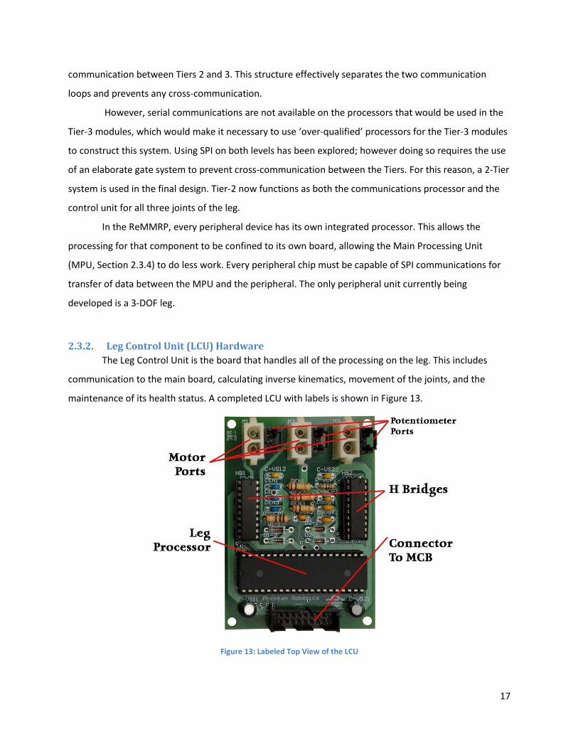
2.3.2. Leg Control Unit (LCU) Hardware The Leg Control Unit is the board that handles all of the processing on the leg. This includes
communication to the main board, calculating inverse kinematics, movement of the joints, and the
maintenance of its health status. A completed LCU with labels is shown in Figure 13.
Figure 13: Labeled Top View of the LCU
18
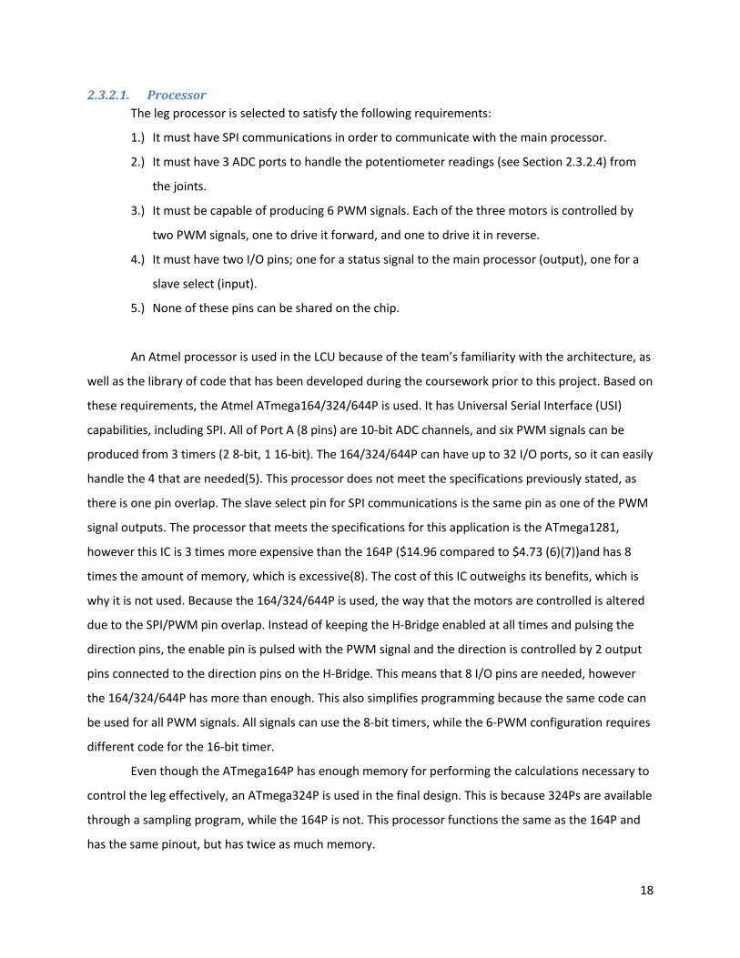
2.3.2.1. Processor The leg processor is selected to satisfy the following requirements:
1.) It must have SPI communications in order to communicate with the main processor.
2.) It must have 3 ADC ports to handle the potentiometer readings (see Section 2.3.2.4) from
the joints.
3.) It must be capable of producing 6 PWM signals. Each of the three motors is controlled by
two PWM signals, one to drive it forward, and one to drive it in reverse.
4.) It must have two I/O pins; one for a status signal to the main processor (output), one for a
slave select (input).
5.) None of these pins can be shared on the chip.
An Atmel processor is used in the LCU because of the team’s familiarity with the architecture, as
well as the library of code that has been developed during the coursework prior to this project. Based on
these requirements, the Atmel ATmega164/324/644P is used. It has Universal Serial Interface (USI)
capabilities, including SPI. All of Port A (8 pins) are 10-bit ADC channels, and six PWM signals can be
produced from 3 timers (2 8-bit, 1 16-bit). The 164/324/644P can have up to 32 I/O ports, so it can easily
handle the 4 that are needed(5). This processor does not meet the specifications previously stated, as
there is one pin overlap. The slave select pin for SPI communications is the same pin as one of the PWM
signal outputs. The processor that meets the specifications for this application is the ATmega1281,
however this IC is 3 times more expensive than the 164P ($14.96 compared to $4.73 (6)(7))and has 8
times the amount of memory, which is excessive(8). The cost of this IC outweighs its benefits, which is
why it is not used. Because the 164/324/644P is used, the way that the motors are controlled is altered
due to the SPI/PWM pin overlap. Instead of keeping the H-Bridge enabled at all times and pulsing the
direction pins, the enable pin is pulsed with the PWM signal and the direction is controlled by 2 output
pins connected to the direction pins on the H-Bridge. This means that 8 I/O pins are needed, however
the 164/324/644P has more than enough. This also simplifies programming because the same code can
be used for all PWM signals. All signals can use the 8-bit timers, while the 6-PWM configuration requires
different code for the 16-bit timer.
Even though the ATmega164P has enough memory for performing the calculations necessary to
control the leg effectively, an ATmega324P is used in the final design. This is because 324Ps are available
through a sampling program, while the 164P is not. This processor functions the same as the 164P and
has the same pinout, but has twice as much memory.
19
2.3.2.2. Motors and Motor Driver The PWM signals that are output from the processor cannot source enough current to directly
run the motors, nor are the signals the correct voltage. The maximum ratings for the I/O pins on the
ATmega164P are 5V at 40mA. Therefore, a motor driver is necessary.
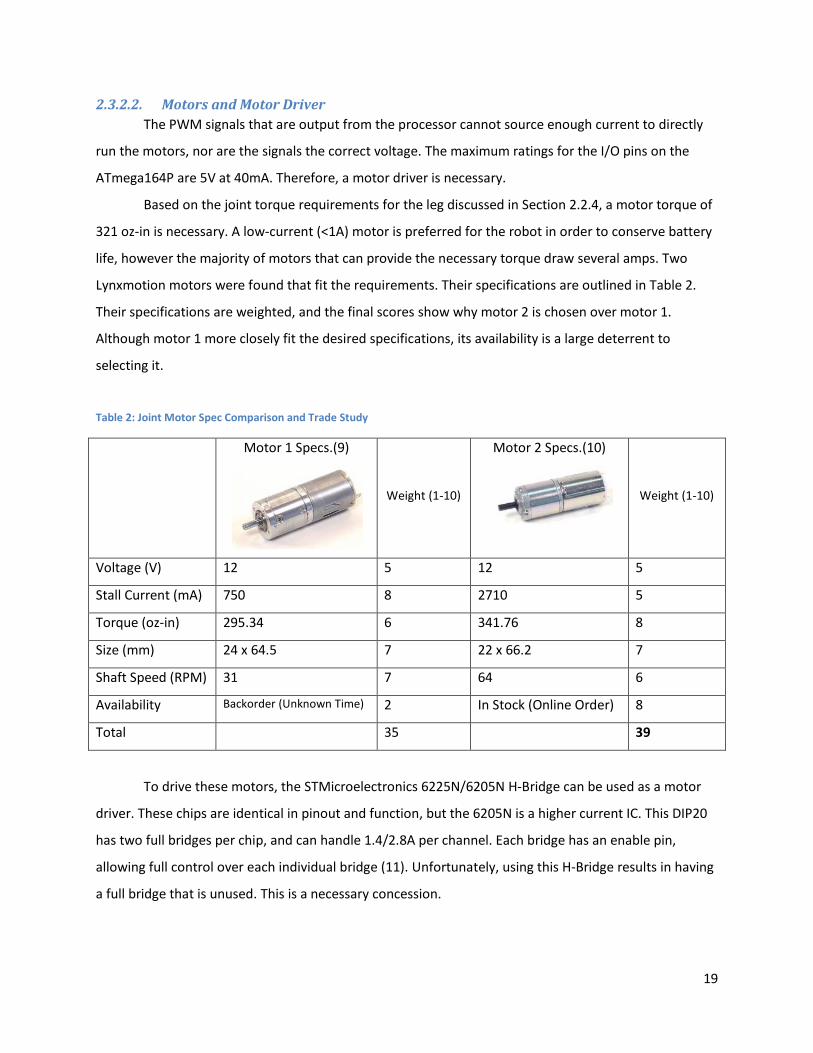
Based on the joint torque requirements for the leg discussed in Section 2.2.4, a motor torque of
321 oz-in is necessary. A low-current (<1A) motor is preferred for the robot in order to conserve battery
life, however the majority of motors that can provide the necessary torque draw several amps. Two
Lynxmotion motors were found that fit the requirements. Their specifications are outlined in Table 2.
Their specifications are weighted, and the final scores show why motor 2 is chosen over motor 1.
Although motor 1 more closely fit the desired specifications, its availability is a large deterrent to
selecting it.
Table 2: Joint Motor Spec Comparison and Trade Study
Motor 1 Specs.(9)
Weight (1-10)
Motor 2 Specs.(10)
Weight (1-10)
Voltage (V) 12 5 12 5
Stall Current (mA) 750 8 2710 5
Torque (oz-in) 295.34 6 341.76 8
Size (mm) 24 x 64.5 7 22 x 66.2 7
Shaft Speed (RPM) 31 7 64 6
Availability Backorder (Unknown Time) 2 In Stock (Online Order) 8
Total 35 39
To drive these motors, the STMicroelectronics 6225N/6205N H-Bridge can be used as a motor
driver. These chips are identical in pinout and function, but the 6205N is a higher current IC. This DIP20
has two full bridges per chip, and can handle 1.4/2.8A per channel. Each bridge has an enable pin,
allowing full control over each individual bridge (11). Unfortunately, using this H-Bridge results in having
a full bridge that is unused. This is a necessary concession.
20
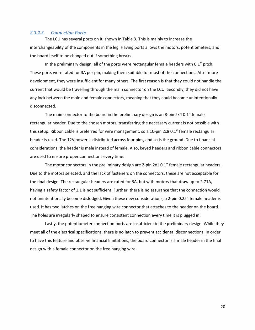
2.3.2.3. Connection Ports The LCU has several ports on it, shown in Table 3. This is mainly to increase the
interchangeability of the components in the leg. Having ports allows the motors, potentiometers, and
the board itself to be changed out if something breaks.
In the preliminary design, all of the ports were rectangular female headers with 0.1” pitch.
These ports were rated for 3A per pin, making them suitable for most of the connections. After more
development, they were insufficient for many others. The first reason is that they could not handle the
current that would be travelling through the main connector on the LCU. Secondly, they did not have
any lock between the male and female connectors, meaning that they could become unintentionally
disconnected.
The main connector to the board in the preliminary design is an 8-pin 2x4 0.1” female
rectangular header. Due to the chosen motors, transferring the necessary current is not possible with
this setup. Ribbon cable is preferred for wire management, so a 16-pin 2x8 0.1” female rectangular
header is used. The 12V power is distributed across four pins, and so is the ground. Due to financial
considerations, the header is male instead of female. Also, keyed headers and ribbon cable connectors
are used to ensure proper connections every time.
The motor connectors in the preliminary design are 2-pin 2x1 0.1” female rectangular headers.
Due to the motors selected, and the lack of fasteners on the connectors, these are not acceptable for
the final design. The rectangular headers are rated for 3A, but with motors that draw up to 2.71A,
having a safety factor of 1.1 is not sufficient. Further, there is no assurance that the connection would
not unintentionally become dislodged. Given these new considerations, a 2-pin 0.25” female header is
used. It has two latches on the free hanging wire connector that attaches to the header on the board.
The holes are irregularly shaped to ensure consistent connection every time it is plugged in.
Lastly, the potentiometer connection ports are insufficient in the preliminary design. While they
meet all of the electrical specifications, there is no latch to prevent accidental disconnections. In order
to have this feature and observe financial limitations, the board connector is a male header in the final
design with a female connector on the free hanging wire.
21
Table 3: Graphic Comparison of LCU Connectors (12)(13)(14)(15)(16)(17)
Motor Connector Potentiometer Connector Main Connector
Preliminary
Final
2.3.2.4. Joint Position Sensing Each joint on the leg module needs a sensor to determine the location of the joint so that it can
be moved to the appropriate location. There are two main options for absolute position sensing. The
first is an absolute encoder. This sensor uses either optical or magnetic sensors to determine its angular
position based on a binary code inside the sensor. The downside to this sensor is that it is very expensive
to use at 10 bits of resolution, which is what the ATmega164/324/644P converts analog signals to using
its ADC.
The other option is a potentiometer. This is an analog sensor that acts as a variable resistor,
varying the output voltage linearly as the angular position changes. They also tend to be less expensive,
and can be more accurate, depending on the quality of the potentiometer. For primarily the cost
benefits, it was decided to use potentiometers.
22
High resistance potentiometers are used so that the current draw is minimized, conserving
battery life. Also, a high quality potentiometer is desired for precision position sensing. Lastly, a small
form factor is necessary so that it does not protrude very far from the leg.
For these reasons, a 10K, 20%, 1-Turn, 53 Series potentiometer from Bourns, Inc. is used on the
leg module. It is in a small package, only 0.521" L x 0.492" W x 0.350" H (18). This potentiometer
functions very well on the leg module.
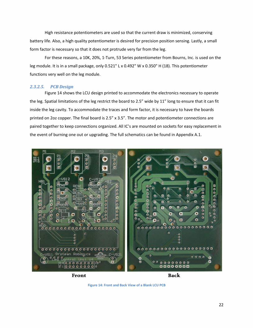
2.3.2.5. PCB Design Figure 14 shows the LCU design printed to accommodate the electronics necessary to operate
the leg. Spatial limitations of the leg restrict the board to 2.5” wide by 11” long to ensure that it can fit
inside the leg cavity. To accommodate the traces and form factor, it is necessary to have the boards
printed on 2oz copper. The final board is 2.5” x 3.5”. The motor and potentiometer connections are
paired together to keep connections organized. All IC’s are mounted on sockets for easy replacement in
the event of burning one out or upgrading. The full schematics can be found in Appendix A.1.
Figure 14: Front and Back View of a Blank LCU PCB
23
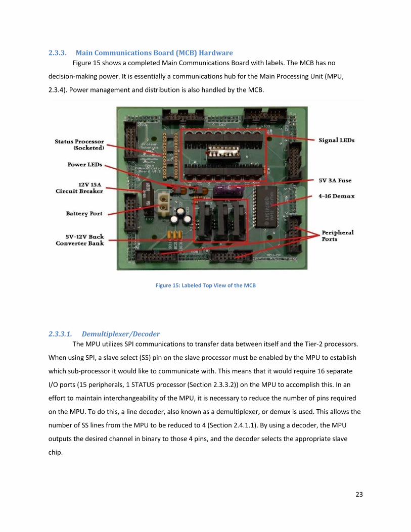
2.3.3. Main Communications Board (MCB) Hardware Figure 15 shows a completed Main Communications Board with labels. The MCB has no
decision-making power. It is essentially a communications hub for the Main Processing Unit (MPU,
2.3.4). Power management and distribution is also handled by the MCB.
Figure 15: Labeled Top View of the MCB
2.3.3.1. Demultiplexer/Decoder The MPU utilizes SPI communications to transfer data between itself and the Tier-2 processors.
When using SPI, a slave select (SS) pin on the slave processor must be enabled by the MPU to establish
which sub-processor it would like to communicate with. This means that it would require 16 separate
I/O ports (15 peripherals, 1 STATUS processor (Section 2.3.3.2)) on the MPU to accomplish this. In an
effort to maintain interchangeability of the MPU, it is necessary to reduce the number of pins required
on the MPU. To do this, a line decoder, also known as a demultiplexer, or demux is used. This allows the
number of SS lines from the MPU to be reduced to 4 (Section 2.4.1.1). By using a decoder, the MPU
outputs the desired channel in binary to those 4 pins, and the decoder selects the appropriate slave
chip.
24
The SN74154N from Texas Instruments is used as the decoder for the ReMMRP. It is a 4-16
decoder. It is also a 5V IC, which is the operating voltage of the other processors, and has a maximum
current draw of 1µA, meaning low power consumption (19).
This decoder allows for the selection of one of 15 peripherals or the STATUS chip, for a total of
16 slaves. 12 of these peripherals will be along the outer edge of the body, and the remaining three will
be available for Internal Connection Ports (ICP), intended for use with sensors internal to the chassis,
such as inertial navigation sensors.
2.3.3.2. STATUS Processor The STATUS (STatus of Attached UnitS) processor is responsible for enumerating peripheral
modules attached to the system and reporting any changes to the MPU. It also is used in the
initialization sequence of the robot to establish which ports have peripherals attached. This processor
has three requirements.
1.) It must have SPI communications for conveying data to the MPU.
2.) It must have 17 I/O ports; 15 for status inputs form the peripherals, one for slave select, and
one for a status change pin to the MPU.
3.) None of these pins can be shared on the chip.
Due to the fact that 22 pins are necessary, a processor with extraneous features must be
selected so that the requisite number of pins are available. The Atmel ATtiny48 meets the requirements
outlined above, and is used as the STATUS chip. It has 24 I/O pins, and has SPI that does not interfere
with the I/O ports for the status inputs (20).
2.3.3.3. Power Management The motors will be running at 12 volts DC, so a 12V DC battery will be used as the power source
for the robot. All of the ICs run at 5V DC, so power must be converted for these chips. The converter
must:
1.) be efficient to conserve the battery life.
2.) be able to provide enough current to run the chips and potentiometers.
3.) reduce the voltage from 12v DC to 5v DC.
25
Using a step-down DC-DC (also known as buck) converter will help with the efficiency. A voltage
regulator is very inefficient because it sheds the excess voltage as heat (21). For the ReMMRP, voltage
will be reduced to 5V from 12V. Assuming the current is constant, a linear regulator operates at the
following efficiency:
5𝑉𝑉12𝑉𝑉
= 41.6%
The IV1205DA from XP Power is used for the power conversion in the preliminary design. It
operates at 74% efficiency, and can supply up to 200mA of current (22). This specification meets the
power to supply requirements by all of the ICs and the leg potentiometers. The leg potentiometers in a
12-leg configuration would consume 18 mA.
In order to account for future peripherals, three 1A DC-DC converters are used in parallel in the
final design. This will allow for high draw peripherals to be developed without having to worry about not
being able to source the necessary current. The Texas Instruments 5101N DC-DC converter is used on
the MCB. It is 90%+ efficient, and can supply 1A of current and has very simple required external
circuitry (23).
Both the 12-volt and the 5-volt lines have current protection. The 12-volt line has a 15A circuit
breaker, and the 5V line has a 3A fuse. A fuse is used for the 5-volt line because it is much less likely that
this line will have a surge of current. The 15A breaker is used because stalling motors can draw large
amounts of current that could damage the board, and using a circuit breaker instead of a fuse saves
time and money by not having to replace it every time it trips.
2.3.3.4. Connection Ports The peripheral ports on the MCB need to meet the same requirements as the 16-pin keyed
rectangular male pin headers on the LCU, and use the same component (Section 2.3.2.3). All 15 of the
peripheral connection ports use this 16-pin header. The port to the MPU will be a 12x1 female header
with 0.1” pitch. This header contains both power and communications lines. The battery connection
port is identical to the one being used for the motors – a 0.25” 2-pin connector with two fastening
latches. This can be used for the battery and the motors because it exceeds the current requirements
for the motor application.
2.3.3.5. Signal LEDs There are 18 signal LEDs on the MPU. These are used to display information to the user. 16 are
status LEDs from peripherals. These are arranged in four 4-LED banks, using a bussed 10K resistor bank
26
as a pull-up resistor. An individual resistor had to be used for the 16th LED as a DIP16 resistor bank only
has 15 available resistors. These LEDs are connected to the status lines from each peripheral port. This
will tell the user which ports have connected peripherals. The other two LEDs are power LEDs, signaling
whether the 5- and 12-volt lines are functioning properly. These also have 10K resistors as pull-up
resistors.
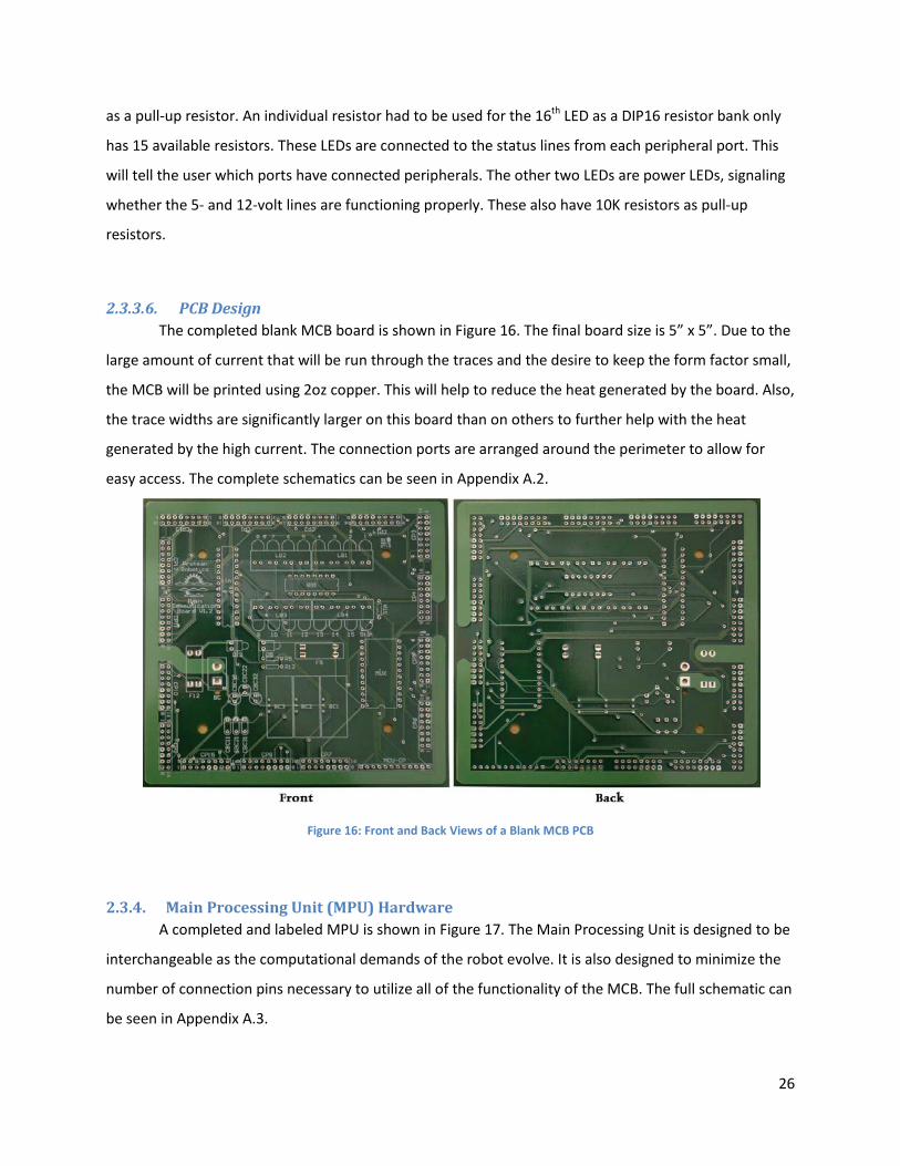
2.3.3.6. PCB Design The completed blank MCB board is shown in Figure 16. The final board size is 5” x 5”. Due to the
large amount of current that will be run through the traces and the desire to keep the form factor small,
the MCB will be printed using 2oz copper. This will help to reduce the heat generated by the board. Also,
the trace widths are significantly larger on this board than on others to further help with the heat
generated by the high current. The connection ports are arranged around the perimeter to allow for
easy access. The complete schematics can be seen in Appendix A.2.
Figure 16: Front and Back Views of a Blank MCB PCB
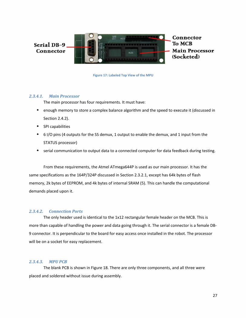
2.3.4. Main Processing Unit (MPU) Hardware A completed and labeled MPU is shown in Figure 17. The Main Processing Unit is designed to be
interchangeable as the computational demands of the robot evolve. It is also designed to minimize the
number of connection pins necessary to utilize all of the functionality of the MCB. The full schematic can
be seen in Appendix A.3.
27
Figure 17: Labeled Top View of the MPU
2.3.4.1. Main Processor The main processor has four requirements. It must have:
enough memory to store a complex balance algorithm and the speed to execute it (discussed in
Section 2.4.2).
SPI capabilities
6 I/O pins (4 outputs for the SS demux, 1 output to enable the demux, and 1 input from the
STATUS processor)
serial communication to output data to a connected computer for data feedback during testing.
From these requirements, the Atmel ATmega644P is used as our main processor. It has the
same specifications as the 164P/324P discussed in Section 2.3.2.1, except has 64k bytes of flash
memory, 2k bytes of EEPROM, and 4k bytes of internal SRAM (5). This can handle the computational
demands placed upon it.
2.3.4.2. Connection Ports The only header used is identical to the 1x12 rectangular female header on the MCB. This is
more than capable of handling the power and data going through it. The serial connector is a female DB-
9 connector. It is perpendicular to the board for easy access once installed in the robot. The processor
will be on a socket for easy replacement.
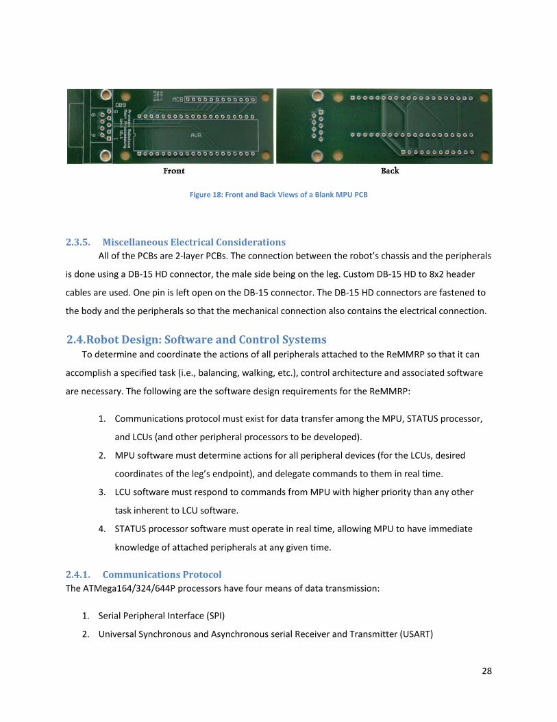
2.3.4.3. MPU PCB The blank PCB is shown in Figure 18. There are only three components, and all three were
placed and soldered without issue during assembly.
28
Figure 18: Front and Back Views of a Blank MPU PCB
2.3.5. Miscellaneous Electrical Considerations All of the PCBs are 2-layer PCBs. The connection between the robot’s chassis and the peripherals
is done using a DB-15 HD connector, the male side being on the leg. Custom DB-15 HD to 8x2 header
cables are used. One pin is left open on the DB-15 connector. The DB-15 HD connectors are fastened to
the body and the peripherals so that the mechanical connection also contains the electrical connection.
2.4. Robot Design: Software and Control Systems To determine and coordinate the actions of all peripherals attached to the ReMMRP so that it can
accomplish a specified task (i.e., balancing, walking, etc.), control architecture and associated software
are necessary. The following are the software design requirements for the ReMMRP:
1. Communications protocol must exist for data transfer among the MPU, STATUS processor,
and LCUs (and other peripheral processors to be developed).
2. MPU software must determine actions for all peripheral devices (for the LCUs, desired
coordinates of the leg’s endpoint), and delegate commands to them in real time.
3. LCU software must respond to commands from MPU with higher priority than any other
task inherent to LCU software.
4. STATUS processor software must operate in real time, allowing MPU to have immediate
knowledge of attached peripherals at any given time.
2.4.1. Communications Protocol The ATMega164/324/644P processors have four means of data transmission:
1. Serial Peripheral Interface (SPI)
2. Universal Synchronous and Asynchronous serial Receiver and Transmitter (USART)
29
3. USART in SPI mode
4. Two Wire Interface (TWI)
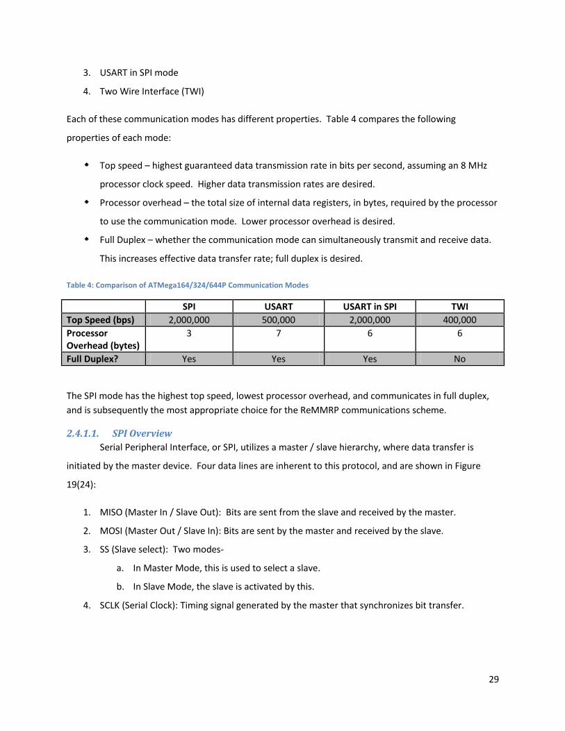
Each of these communication modes has different properties. Table 4 compares the following
properties of each mode:
Top speed – highest guaranteed data transmission rate in bits per second, assuming an 8 MHz
processor clock speed. Higher data transmission rates are desired.
Processor overhead – the total size of internal data registers, in bytes, required by the processor
to use the communication mode. Lower processor overhead is desired.
Full Duplex – whether the communication mode can simultaneously transmit and receive data.
This increases effective data transfer rate; full duplex is desired.
Table 4: Comparison of ATMega164/324/644P Communication Modes
SPI USART USART in SPI TWI Top Speed (bps) 2,000,000 500,000 2,000,000 400,000 Processor Overhead (bytes)
3 7 6 6
Full Duplex? Yes Yes Yes No
The SPI mode has the highest top speed, lowest processor overhead, and communicates in full duplex, and is subsequently the most appropriate choice for the ReMMRP communications scheme.
2.4.1.1. SPI Overview Serial Peripheral Interface, or SPI, utilizes a master / slave hierarchy, where data transfer is
initiated by the master device. Four data lines are inherent to this protocol, and are shown in Figure
19(24):
1. MISO (Master In / Slave Out): Bits are sent from the slave and received by the master.
2. MOSI (Master Out / Slave In): Bits are sent by the master and received by the slave.
3. SS (Slave select): Two modes-
a. In Master Mode, this is used to select a slave.
b. In Slave Mode, the slave is activated by this.
4. SCLK (Serial Clock): Timing signal generated by the master that synchronizes bit transfer.
30
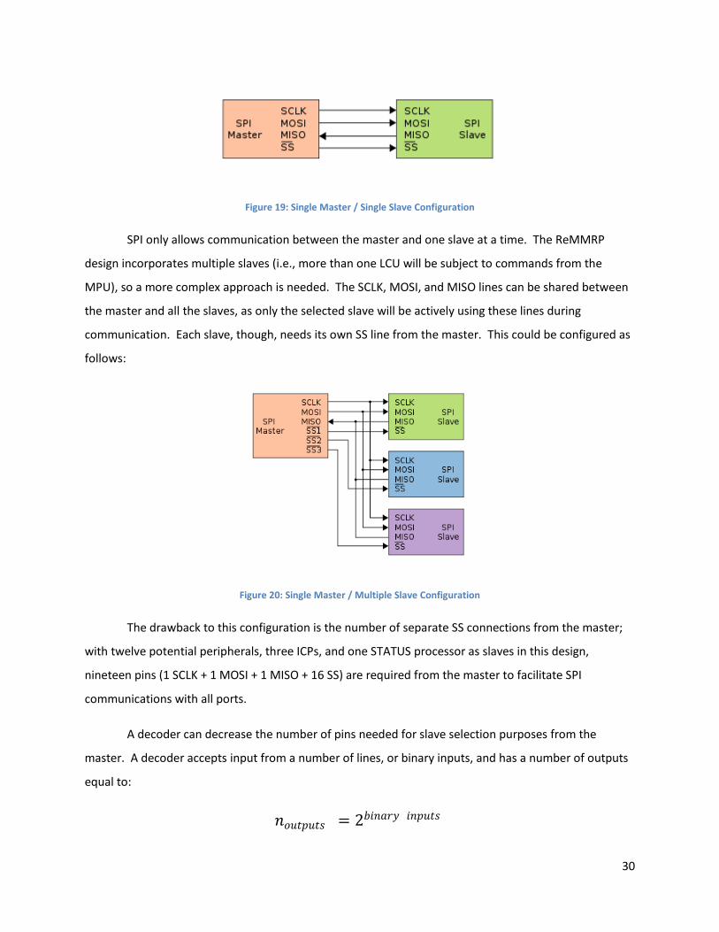
Figure 19: Single Master / Single Slave Configuration
SPI only allows communication between the master and one slave at a time. The ReMMRP
design incorporates multiple slaves (i.e., more than one LCU will be subject to commands from the
MPU), so a more complex approach is needed. The SCLK, MOSI, and MISO lines can be shared between
the master and all the slaves, as only the selected slave will be actively using these lines during
communication. Each slave, though, needs its own SS line from the master. This could be configured as
follows:
Figure 20: Single Master / Multiple Slave Configuration
The drawback to this configuration is the number of separate SS connections from the master;
with twelve potential peripherals, three ICPs, and one STATUS processor as slaves in this design,
nineteen pins (1 SCLK + 1 MOSI + 1 MISO + 16 SS) are required from the master to facilitate SPI
communications with all ports.
A decoder can decrease the number of pins needed for slave selection purposes from the
master. A decoder accepts input from a number of lines, or binary inputs, and has a number of outputs
equal to:
𝑖𝑖𝑜𝑜𝑜𝑜𝑜𝑜𝑜𝑜𝑜𝑜𝑜𝑜𝑜𝑜 = 2𝑏𝑏𝑖𝑖𝑖𝑖𝑏𝑏𝑏𝑏𝑏𝑏 𝑖𝑖𝑖𝑖𝑜𝑜𝑜𝑜𝑜𝑜𝑜𝑜
31
The decoder selected for this design (Section 2.3.3.1) has sixteen outputs, and will activate the
output that corresponds to the value of the 4-bit input signal. This way, a four line signal can be used to
activate one of sixteen peripherals, reducing the master’s SPI pin requirements to seven (1 SCLK + 1
MOSI + 1 MISO + 4 Binary Signal to Decoder).
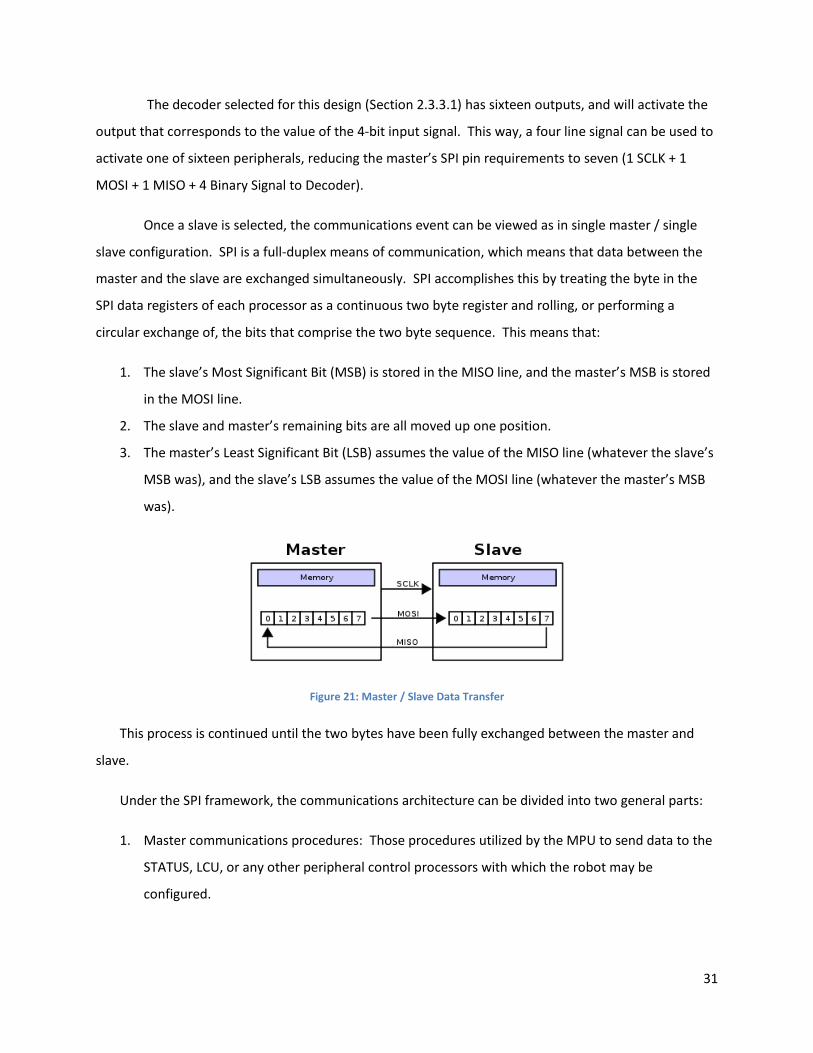
Once a slave is selected, the communications event can be viewed as in single master / single
slave configuration. SPI is a full-duplex means of communication, which means that data between the
master and the slave are exchanged simultaneously. SPI accomplishes this by treating the byte in the
SPI data registers of each processor as a continuous two byte register and rolling, or performing a
circular exchange of, the bits that comprise the two byte sequence. This means that:
1. The slave’s Most Significant Bit (MSB) is stored in the MISO line, and the master’s MSB is stored
in the MOSI line.
2. The slave and master’s remaining bits are all moved up one position.
3. The master’s Least Significant Bit (LSB) assumes the value of the MISO line (whatever the slave’s
MSB was), and the slave’s LSB assumes the value of the MOSI line (whatever the master’s MSB
was).
Figure 21: Master / Slave Data Transfer
This process is continued until the two bytes have been fully exchanged between the master and
slave.
Under the SPI framework, the communications architecture can be divided into two general parts:
1. Master communications procedures: Those procedures utilized by the MPU to send data to the
STATUS, LCU, or any other peripheral control processors with which the robot may be
configured.
32
2. Slave communications procedures: Those procedures utilized by the STATUS, LCU, or any other
peripheral control processors with which the robot may be configured, to send data to and
receive data from the master processor.
Since SPI utilizes a full-duplex communications mode with a clock, sending and receiving are done
not only simultaneously but also synchronously. The data exchange is quantified on the byte level, and
initiated only by the master. Therefore, the above generalization defines a communication session as:
1. Master communications procedures:
a. Select slave
b. Choose byte to send
c. Send byte, receive byte from slave
d. Unselect slave
2. Slave communications procedures:
a. Wait for selection from master
b. Exchange current stored byte with incoming byte from master
In an episodic sense, these procedures do not appear to be an effective means of transferring
information. Since communication between the master and slave at a given time involves the transfer
of multiple bytes, an additional layer of abstraction over the SPI communication protocol is
implemented.
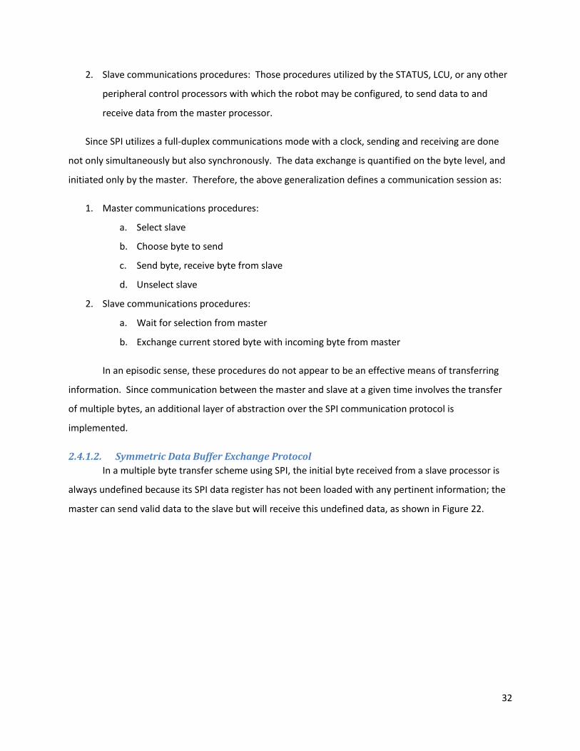
2.4.1.2. Symmetric Data Buffer Exchange Protocol In a multiple byte transfer scheme using SPI, the initial byte received from a slave processor is
always undefined because its SPI data register has not been loaded with any pertinent information; the
master can send valid data to the slave but will receive this undefined data, as shown in Figure 22.
33
Figure 22: SPI Initial Single Byte Data Exchange
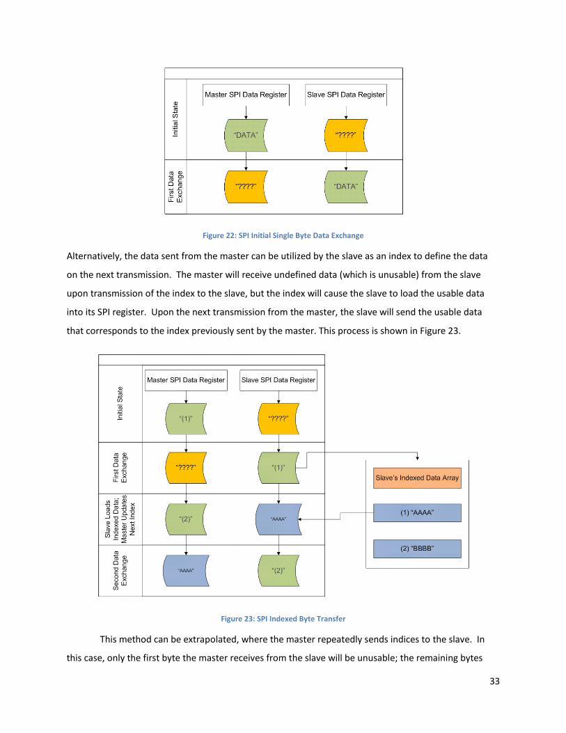
Alternatively, the data sent from the master can be utilized by the slave as an index to define the data
on the next transmission. The master will receive undefined data (which is unusable) from the slave
upon transmission of the index to the slave, but the index will cause the slave to load the usable data
into its SPI register. Upon the next transmission from the master, the slave will send the usable data
that corresponds to the index previously sent by the master. This process is shown in Figure 23.
Figure 23: SPI Indexed Byte Transfer
This method can be extrapolated, where the master repeatedly sends indices to the slave. In
this case, only the first byte the master receives from the slave will be unusable; the remaining bytes
34
received will be pertinent information from the slave. The last byte the master sends does not need any
particular value in order to receive the last byte of indexed data from the slave. Note that this process
results in a data offset between the master and slave; the master is always one byte behind the slave in
terms of the byte sequence.
The indices sent from the master are useful in requesting data from the slave, but have no
particular meaning to the overall operation of the robot other than to ensure the proper data is received
from the slave processor. The communications session would be better exploited if more pertinent data
were exchanged as often as possible. To accomplish this, data buffers must exist on both the master
and slave processors in the following manner:
1. Each element in the data buffer must be a single byte, commensurate with the size of the SPI
register.
2. The data buffers present on the slave must be known by the master and each buffer must have
an index that explicitly identifies it.
3. The size of the data buffers on both processors must be known by the master before
transmission begins. The data buffers to be exchanged must be of equal size; this criterion is
fundamental to the symmetric aspect of this protocol.
4. One buffer is chosen on each processor as a “send” buffer, and one buffer is chosen on each
processor as a “receive” buffer.
With these rules in place, the master and slave can simultaneously transfer information blocks of
equal size. This process will be referred to as Symmetric Data Buffer Exchange (SDBE).
In the following example, the MPU simultaneously sends the LCU new coordinates and receives
from the LCU its last known coordinates using SDBE. The assumption will be made that both processors
have a data buffer called “Command Coordinates,” and the LCU has an additional buffer called “Current
Coordinates.” The data exchange will occur as follows:
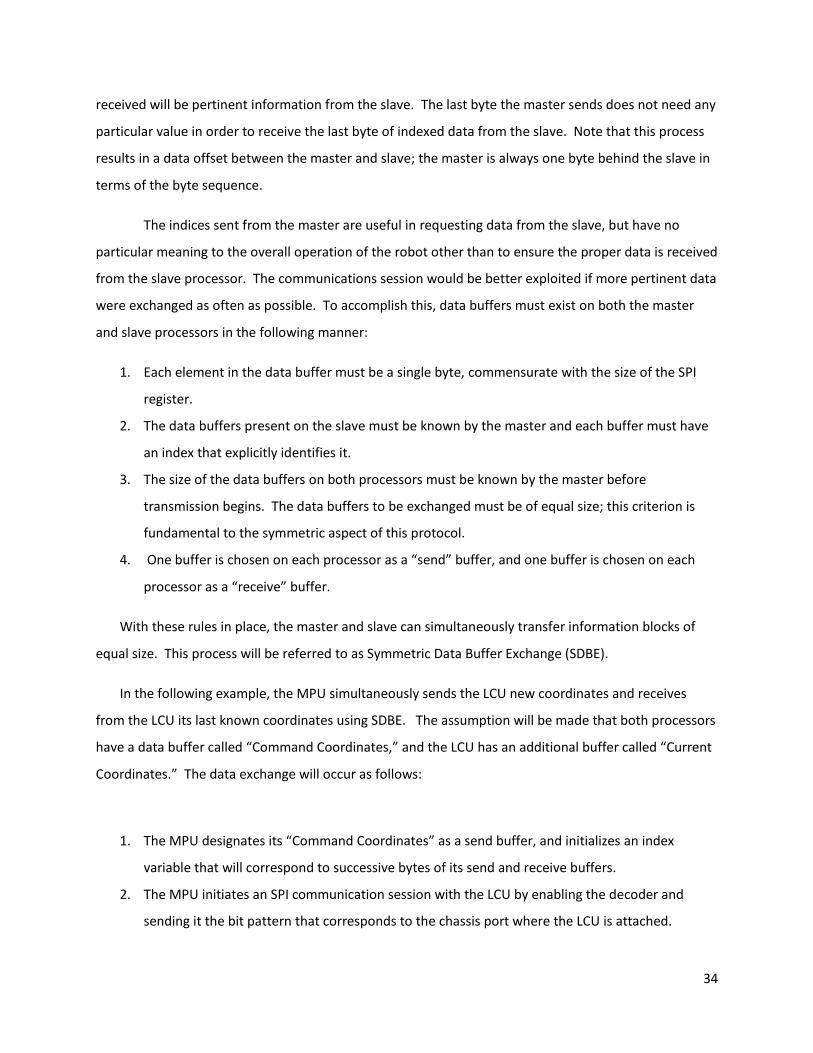
1. The MPU designates its “Command Coordinates” as a send buffer, and initializes an index
variable that will correspond to successive bytes of its send and receive buffers.
2. The MPU initiates an SPI communication session with the LCU by enabling the decoder and
sending it the bit pattern that corresponds to the chassis port where the LCU is attached.
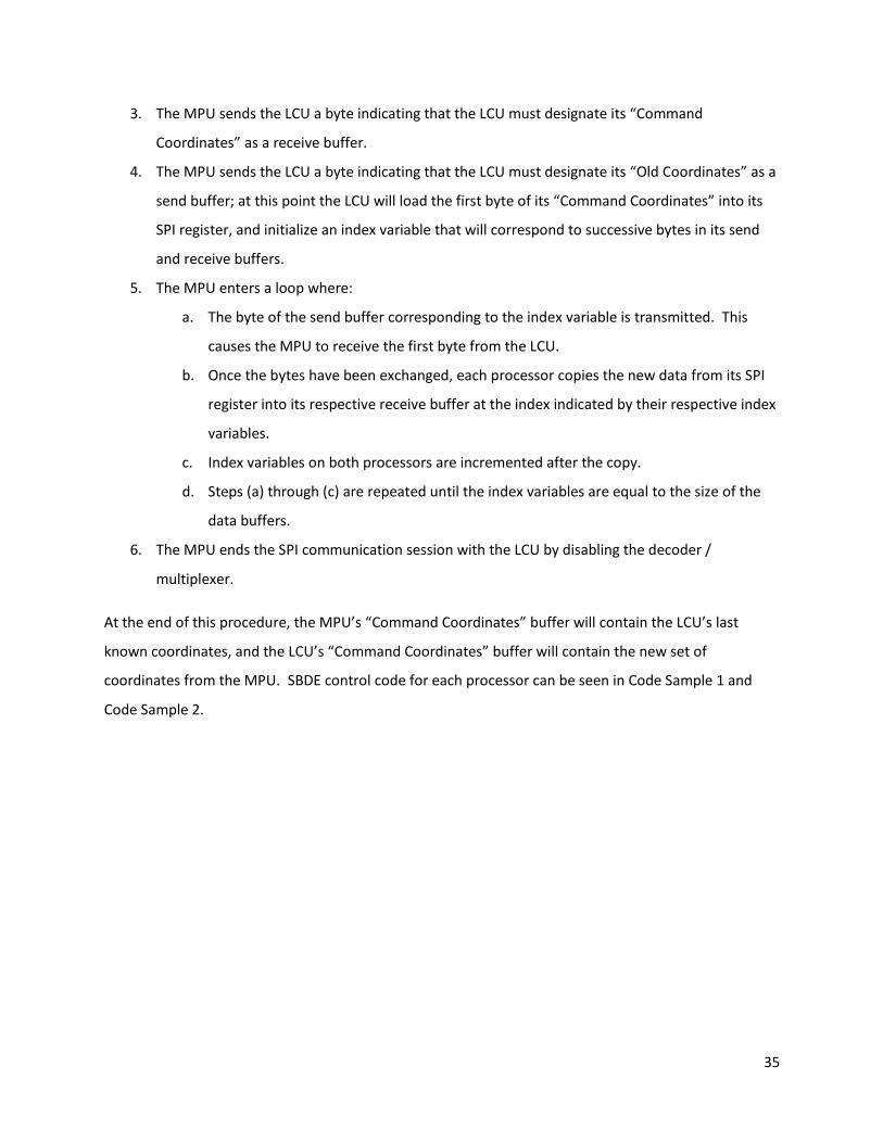
35
3. The MPU sends the LCU a byte indicating that the LCU must designate its “Command
Coordinates” as a receive buffer.
4. The MPU sends the LCU a byte indicating that the LCU must designate its “Old Coordinates” as a
send buffer; at this point the LCU will load the first byte of its “Command Coordinates” into its
SPI register, and initialize an index variable that will correspond to successive bytes in its send
and receive buffers.
5. The MPU enters a loop where:
a. The byte of the send buffer corresponding to the index variable is transmitted. This
causes the MPU to receive the first byte from the LCU.
b. Once the bytes have been exchanged, each processor copies the new data from its SPI
register into its respective receive buffer at the index indicated by their respective index
variables.
c. Index variables on both processors are incremented after the copy.
d. Steps (a) through (c) are repeated until the index variables are equal to the size of the
data buffers.
6. The MPU ends the SPI communication session with the LCU by disabling the decoder /
multiplexer.
At the end of this procedure, the MPU’s “Command Coordinates” buffer will contain the LCU’s last
known coordinates, and the LCU’s “Command Coordinates” buffer will contain the new set of
coordinates from the MPU. SBDE control code for each processor can be seen in Code Sample 1 and
Code Sample 2.
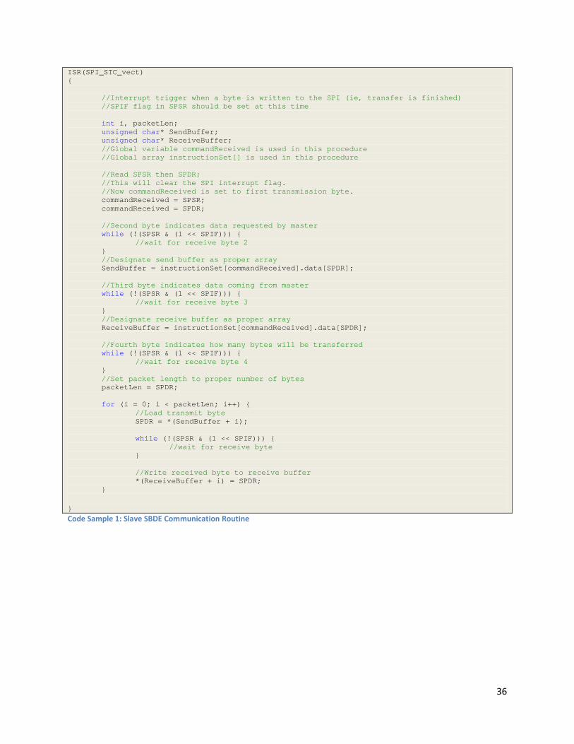
36
ISR(SPI_STC_vect) { //Interrupt trigger when a byte is written to the SPI (ie, transfer is finished) //SPIF flag in SPSR should be set at this time int i, packetLen; unsigned char* SendBuffer; unsigned char* ReceiveBuffer; //Global variable commandReceived is used in this procedure //Global array instructionSet[] is used in this procedure //Read SPSR then SPDR; //This will clear the SPI interrupt flag. //Now commandReceived is set to first transmission byte. commandReceived = SPSR; commandReceived = SPDR; //Second byte indicates data requested by master while (!(SPSR & (1 << SPIF))) { //wait for receive byte 2 } //Designate send buffer as proper array SendBuffer = instructionSet[commandReceived].data[SPDR]; //Third byte indicates data coming from master while (!(SPSR & (1 << SPIF))) { //wait for receive byte 3 } //Designate receive buffer as proper array ReceiveBuffer = instructionSet[commandReceived].data[SPDR]; //Fourth byte indicates how many bytes will be transferred while (!(SPSR & (1 << SPIF))) { //wait for receive byte 4 } //Set packet length to proper number of bytes packetLen = SPDR; for (i = 0; i < packetLen; i++) { //Load transmit byte SPDR = *(SendBuffer + i); while (!(SPSR & (1 << SPIF))) { //wait for receive byte } //Write received byte to receive buffer *(ReceiveBuffer + i) = SPDR; } } Code Sample 1: Slave SBDE Communication Routine
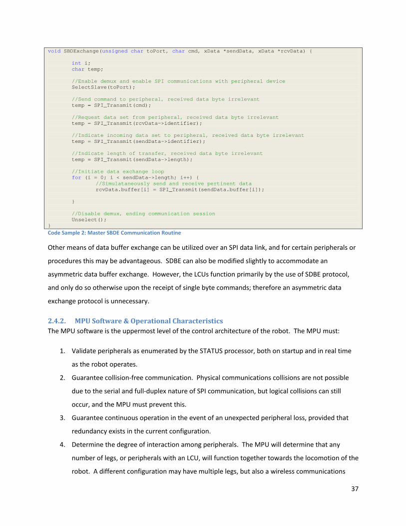
37
void SBDExchange(unsigned char toPort, char cmd, xData *sendData, xData *rcvData) { int i; char temp; //Enable demux and enable SPI communications with peripheral device SelectSlave(toPort); //Send command to peripheral, received data byte irrelevant temp = SPI_Transmit(cmd); //Request data set from peripheral, received data byte irrelevant temp = SPI_Transmit(rcvData->identifier); //Indicate incoming data set to peripheral, received data byte irrelevant temp = SPI_Transmit(sendData->identifier); //Indicate length of transfer, received data byte irrelevant temp = SPI_Transmit(sendData->length); //Initiate data exchange loop for (i = 0; i < sendData->length; i++) { //Simulataneously send and receive pertinent data rcvData.buffer[i] = SPI_Transmit(sendData.buffer[i]); } //Disable demux, ending communication session Unselect(); } Code Sample 2: Master SBDE Communication Routine
Other means of data buffer exchange can be utilized over an SPI data link, and for certain peripherals or
procedures this may be advantageous. SDBE can also be modified slightly to accommodate an
asymmetric data buffer exchange. However, the LCUs function primarily by the use of SDBE protocol,
and only do so otherwise upon the receipt of single byte commands; therefore an asymmetric data
exchange protocol is unnecessary.
2.4.2. MPU Software & Operational Characteristics The MPU software is the uppermost level of the control architecture of the robot. The MPU must:
1. Validate peripherals as enumerated by the STATUS processor, both on startup and in real time
as the robot operates.
2. Guarantee collision-free communication. Physical communications collisions are not possible
due to the serial and full-duplex nature of SPI communication, but logical collisions can still
occur, and the MPU must prevent this.
3. Guarantee continuous operation in the event of an unexpected peripheral loss, provided that
redundancy exists in the current configuration.
4. Determine the degree of interaction among peripherals. The MPU will determine that any
number of legs, or peripherals with an LCU, will function together towards the locomotion of the
robot. A different configuration may have multiple legs, but also a wireless communications
38
beacon. In this situation the MPU must still determine the cooperative relationship that the legs
share, but also determine that the wireless peripheral has a separate and independent function.
5. Control peripherals at their degree of interaction.
The above functions will now be discussed in further detail.
2.4.2.1. Peripheral Validation On startup, the MPU must wait for a “ready” signal from the STATUS processor. After receiving
this signal, the MPU can poll the STATUS processor for information regarding what ports on the robot
chassis have peripheral devices attached to them. Once the MPU is aware of which ports are active, it
can then poll these ports for information.
Every peripheral device will have a serial number written directly into its memory, either as a
constant term in the embedded software, or stored in its permanent EEPROM memory. This serial
number identifies the peripheral as a particular type of device, and the MPU will have a list of every
possible peripheral. The MPU will initially request this information from each peripheral, and create a
data structure for each port that corresponds to the device that is attached there.
2.4.2.2. Communications The MPU acts as the master in communications with all other processors in the robot
architecture. As such, it is responsible for initiating any and all communications. In a multiprocessor
environment, care must be taken to avoid collisions in data transfer. The primary type of data collision
in computer networking is a physical collision; this occurs when data transfer occurs simultaneously
between more than two processors (25). The SPI protocol is free from this concern in a single master /
multiple slave environment.
A secondary type of collision will be referred to hereafter as a logical collision. This is likely
inherent to other architectures, but for the purposes of this paper it will pertain solely to the robotic
design of this project. Logical collision potential exists when the MPU attempts to exchange data with a
peripheral before that peripheral has utilized the most recent data that was exchanged.
In the case of the SDBE protocol, this might occur if:
The MPU exchanges a number of bytes of data with an LCU, indicating a set of coordinates.
The LCU begins using this new data, but the master sends another set of coordinates half way
through the LCU’s procedures having to do with said data.
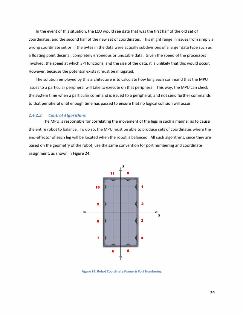
39
In the event of this situation, the LCU would see data that was the first half of the old set of
coordinates, and the second half of the new set of coordinates. This might range in issues from simply a
wrong coordinate set or, if the bytes in the data were actually subdivisions of a larger data type such as
a floating point decimal, completely erroneous or unusable data. Given the speed of the processors
involved, the speed at which SPI functions, and the size of the data, it is unlikely that this would occur.
However, because the potential exists it must be mitigated.
The solution employed by this architecture is to calculate how long each command that the MPU
issues to a particular peripheral will take to execute on that peripheral. This way, the MPU can check
the system time when a particular command is issued to a peripheral, and not send further commands
to that peripheral until enough time has passed to ensure that no logical collision will occur.
2.4.2.3. Control Algorithms The MPU is responsible for correlating the movement of the legs in such a manner as to cause
the entire robot to balance. To do so, the MPU must be able to produce sets of coordinates where the
end-effector of each leg will be located when the robot is balanced. All such algorithms, since they are
based on the geometry of the robot, use the same convention for port numbering and coordinate
assignment, as shown in Figure 24:
Figure 24: Robot Coordinate Frame & Port Numbering
40
The robot coordinate frame’s origin is positioned at the geometric center of the robot chassis,
with the long edges parallel to the y-axis, and the short edges parallel to the x-axis, as viewed from
above the robot. Using the right-hand rule, the z-axis extends skyward from the robot chassis center.
The ports are numbered beginning with “0” at the topmost right in this orientation and increasing
clockwise until “11”. Any positional coordinate of the robot’s peripherals can ultimately be expressed in
terms of this system, and the balancing algorithms described below use that fact advantageously.
Combined Static Stability and Mobility (CoSSMo) Balancing Method
This method of balancing is done without the benefit of accelerometers or gyroscopic devices. The
only data utilized is the number of legs attached to the robot and where they are. The following
assumptions are then made:
The center of gravity of the robot is the geometric center of the chassis.
The robot is on a flat surface.
The robot is not in motion.
The robot has been commanded to a set height. This will fix the z-coordinate of the robot
chassis, and calculate a configuration for the robot to stand at the desired height.
This balancing algorithm has two separate goals. These are:
Maximize Stability: Determine most stable configuration as defined by the area of the base of
support, or the polygon made by defining each leg’s end-effector as the vertex of a polygon in
the x-y plane, and the position of the robot’s center of gravity, or mass centroid, when projected
onto this polygon.
Maximize Mobility: Determine the greatest potential for motion from the balanced
configuration, i.e., how much each end-effector is able to move within its workspace from the
balanced position.
The mobility and stability of the robot both depend on the position of the end-effectors, but in most
cases improving one will tend to worsen the other. Therefore the algorithm must find a compromise
between the stability and mobility metrics, where a configuration is found in which the robot is both
statically balanced and has some ability to move each leg in any direction.
One approach to this involves calculating and storing optimal or sufficient solutions for each possible
configuration. However, even with the presumption that the robot cannot balance with less than three
41
legs, the possible configurations can be numbered using the “choose” function. The function �𝑖𝑖𝑥𝑥�, read
as “n choose x,” determines the number of ways that x elements from an equal or larger set of n
elements can be arranged. This function is calculated as follows:
Equation 5: Choose Function
�𝑖𝑖𝑥𝑥� =𝑖𝑖!
𝑥𝑥! (𝑖𝑖 − 𝑥𝑥)!
Since the ReMMRP has a twelve-port chassis, n will always be fixed to 12 (the number of ports
cannot be changed). The variable x will denote how many legs are attached in a given configuration.
The robot cannot physically balance with less than 3 legs attached; therefore 1 and 2 leg configurations
will not be explored.
In the interest of examining search space for the algorithm, the choose function can be utilized
to express the number of configurations the robot can have with different numbers of legs. Beginning
with the least allowable number of legs, the number of different configurations possible can be stated as
“12 choose 3,” and calculated as:
�123 � =
12!3! (12 − 3)!
= 220
Extrapolating this to the remaining possible number of legs (4 through 12) and summing the
results, the total configurations possible for the range 3 to 12 legs is:
Equation 6: Total Possible Leg Configurations of ReMMRP
��12𝑖𝑖 �
12
𝑖𝑖=3
= �12!
𝑖𝑖! (12 − 𝑖𝑖)!
12
𝑖𝑖=3
= 4017
Pre-calculating, optimizing, and storing this amount of possible configurations would still be a
heavily time consuming and storage intensive task. The robot uses an 8MHz main processor with 4K of
RAM, so the space and time complexity of the algorithm must remain very small in order to function at
all. Therefore, the candidate algorithm must be small enough to fit in the 64K of processor memory, and
fast enough to calculate a “good” balance scheme in a small amount of time, with a processor that is
very slow by modern standards. The CoSSMo algorithm is a rudimentary but effective solution to the
compromise between stability and mobility.
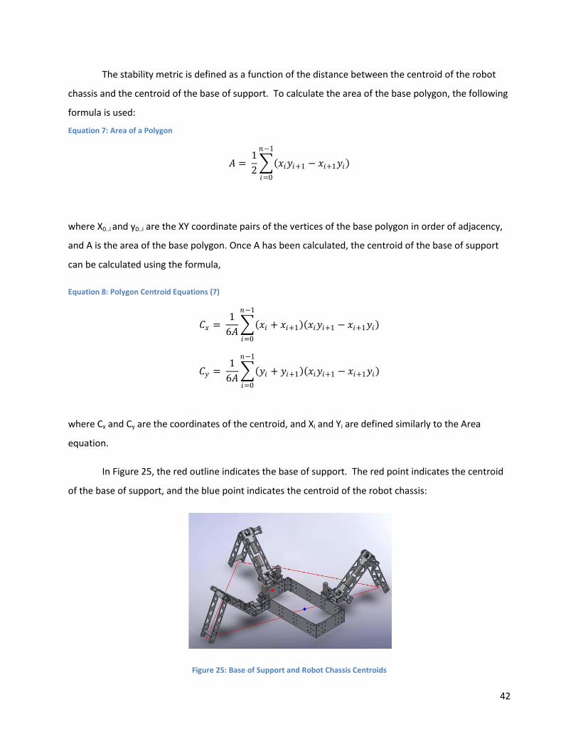
42
The stability metric is defined as a function of the distance between the centroid of the robot
chassis and the centroid of the base of support. To calculate the area of the base polygon, the following
formula is used:
Equation 7: Area of a Polygon
𝐴𝐴 = 12�(𝑥𝑥𝑖𝑖𝑏𝑏𝑖𝑖+1 − 𝑥𝑥𝑖𝑖+1𝑏𝑏𝑖𝑖)𝑖𝑖−1
𝑖𝑖=0
where X0..i and y0..i are the XY coordinate pairs of the vertices of the base polygon in order of adjacency,
and A is the area of the base polygon. Once A has been calculated, the centroid of the base of support
can be calculated using the formula,
Equation 8: Polygon Centroid Equations (7)
𝐶𝐶𝑥𝑥 = 1
6𝐴𝐴�(𝑥𝑥𝑖𝑖 + 𝑥𝑥𝑖𝑖+1)(𝑥𝑥𝑖𝑖𝑏𝑏𝑖𝑖+1 − 𝑥𝑥𝑖𝑖+1𝑏𝑏𝑖𝑖)𝑖𝑖−1
𝑖𝑖=0
𝐶𝐶𝑏𝑏 = 1
6𝐴𝐴�(𝑏𝑏𝑖𝑖 + 𝑏𝑏𝑖𝑖+1)(𝑥𝑥𝑖𝑖𝑏𝑏𝑖𝑖+1 − 𝑥𝑥𝑖𝑖+1𝑏𝑏𝑖𝑖)𝑖𝑖−1
𝑖𝑖=0
where Cx and Cy are the coordinates of the centroid, and Xi and Yi are defined similarly to the Area
equation.
In Figure 25, the red outline indicates the base of support. The red point indicates the centroid
of the base of support, and the blue point indicates the centroid of the robot chassis:
Figure 25: Base of Support and Robot Chassis Centroids
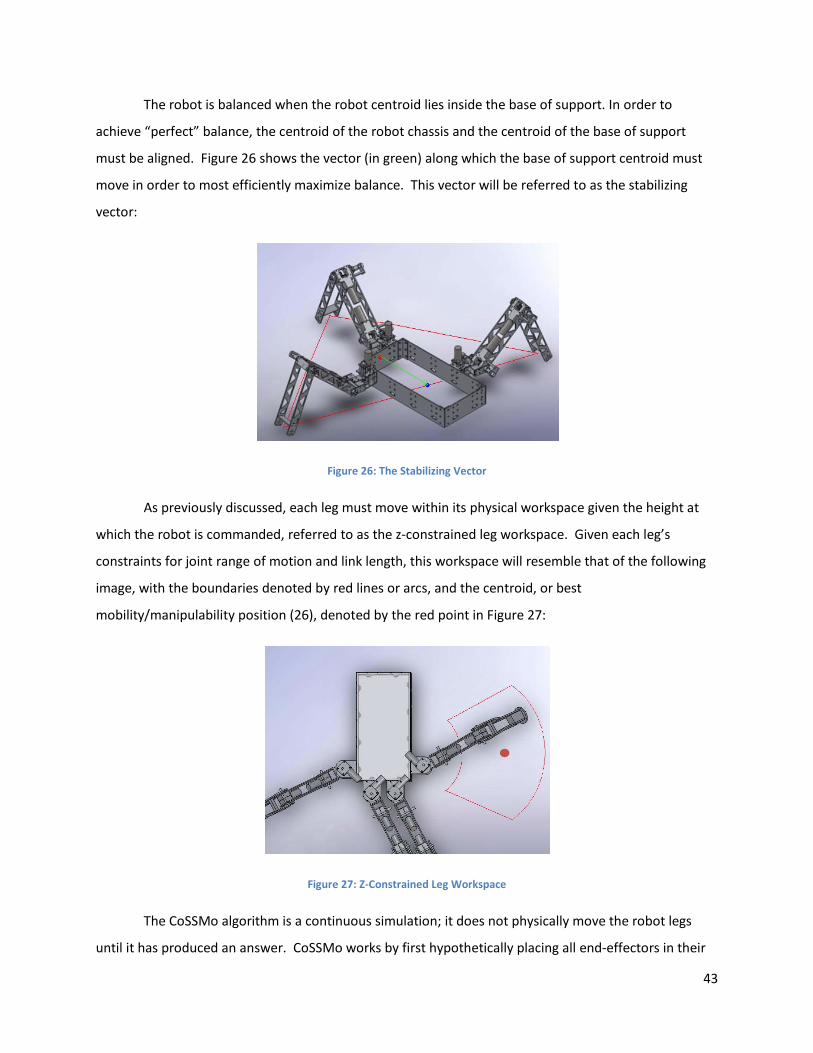
43
The robot is balanced when the robot centroid lies inside the base of support. In order to
achieve “perfect” balance, the centroid of the robot chassis and the centroid of the base of support
must be aligned. Figure 26 shows the vector (in green) along which the base of support centroid must
move in order to most efficiently maximize balance. This vector will be referred to as the stabilizing
vector:
Figure 26: The Stabilizing Vector
As previously discussed, each leg must move within its physical workspace given the height at
which the robot is commanded, referred to as the z-constrained leg workspace. Given each leg’s
constraints for joint range of motion and link length, this workspace will resemble that of the following
image, with the boundaries denoted by red lines or arcs, and the centroid, or best
mobility/manipulability position (26), denoted by the red point in Figure 27:
Figure 27: Z-Constrained Leg Workspace
The CoSSMo algorithm is a continuous simulation; it does not physically move the robot legs
until it has produced an answer. CoSSMo works by first hypothetically placing all end-effectors in their
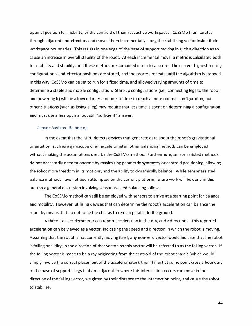
44
optimal position for mobility, or the centroid of their respective workspaces. CoSSMo then iterates
through adjacent end-effectors and moves them incrementally along the stabilizing vector inside their
workspace boundaries. This results in one edge of the base of support moving in such a direction as to
cause an increase in overall stability of the robot. At each incremental move, a metric is calculated both
for mobility and stability, and these metrics are combined into a total score. The current highest scoring
configuration’s end-effector positions are stored, and the process repeats until the algorithm is stopped.
In this way, CoSSMo can be set to run for a fixed time, and allowed varying amounts of time to
determine a stable and mobile configuration. Start-up configurations (i.e., connecting legs to the robot
and powering it) will be allowed larger amounts of time to reach a more optimal configuration, but
other situations (such as losing a leg) may require that less time is spent on determining a configuration
and must use a less optimal but still “sufficient” answer.
Sensor Assisted Balancing
In the event that the MPU detects devices that generate data about the robot’s gravitational
orientation, such as a gyroscope or an accelerometer, other balancing methods can be employed
without making the assumptions used by the CoSSMo method. Furthermore, sensor assisted methods
do not necessarily need to operate by maximizing geometric symmetry or centroid positioning, allowing
the robot more freedom in its motions, and the ability to dynamically balance. While sensor assisted
balance methods have not been attempted on the current platform, future work will be done in this
area so a general discussion involving sensor assisted balancing follows.
The CoSSMo method can still be employed with sensors to arrive at a starting point for balance
and mobility. However, utilizing devices that can determine the robot’s acceleration can balance the
robot by means that do not force the chassis to remain parallel to the ground.
A three-axis accelerometer can report acceleration in the x, y, and z directions. This reported
acceleration can be viewed as a vector, indicating the speed and direction in which the robot is moving.
Assuming that the robot is not currently moving itself, any non-zero vector would indicate that the robot
is falling or sliding in the direction of that vector, so this vector will be referred to as the falling vector. If
the falling vector is made to be a ray originating from the centroid of the robot chassis (which would
simply involve the correct placement of the accelerometer), then it must at some point cross a boundary
of the base of support. Legs that are adjacent to where this intersection occurs can move in the
direction of the falling vector, weighted by their distance to the intersection point, and cause the robot
to stabilize.
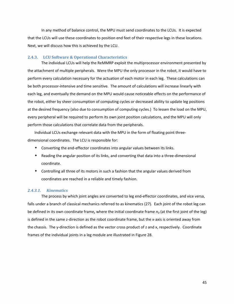
45
In any method of balance control, the MPU must send coordinates to the LCUs. It is expected
that the LCUs will use these coordinates to position end feet of their respective legs in these locations.
Next, we will discuss how this is achieved by the LCU.
2.4.3. LCU Software & Operational Characteristics The individual LCUs will help the ReMMRP exploit the multiprocessor environment presented by
the attachment of multiple peripherals. Were the MPU the only processor in the robot, it would have to
perform every calculation necessary for the actuation of each motor in each leg. These calculations can
be both processor-intensive and time sensitive. The amount of calculations will increase linearly with
each leg, and eventually the demand on the MPU would cause noticeable effects on the performance of
the robot, either by sheer consumption of computing cycles or decreased ability to update leg positions
at the desired frequency (also due to consumption of computing cycles.) To lessen the load on the MPU,
every peripheral will be required to perform its own joint position calculations, and the MPU will only
perform those calculations that correlate data from the peripherals.
Individual LCUs exchange relevant data with the MPU in the form of floating point three-
dimensional coordinates. The LCU is responsible for:
Converting the end-effector coordinates into angular values between its links.
Reading the angular position of its links, and converting that data into a three-dimensional
coordinate.
Controlling all three of its motors in such a fashion that the angular values derived from
coordinates are reached in a reliable and timely fashion.
2.4.3.1. Kinematics The process by which joint angles are converted to leg end-effector coordinates, and vice versa,
falls under a branch of classical mechanics referred to as kinematics (27). Each joint of the robot leg can
be defined in its own coordinate frame, where the initial coordinate frame n0 (at the first joint of the leg)
is defined in the same z-direction as the robot coordinate frame, but the x-axis is oriented away from
the chassis. The y-direction is defined as the vector cross product of z and x, respectively. Coordinate
frames of the individual joints in a leg module are illustrated in Figure 28.
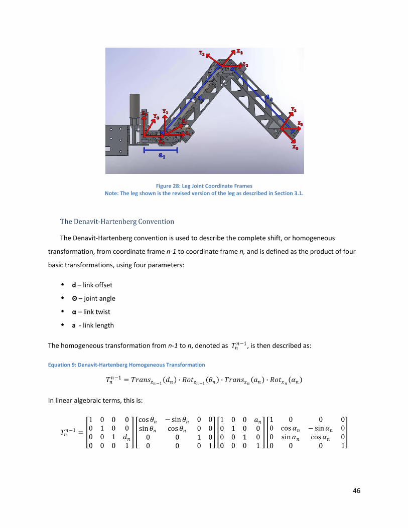
46
Figure 28: Leg Joint Coordinate Frames Note: The leg shown is the revised version of the leg as described in Section 3.1.
The Denavit-Hartenberg Convention
The Denavit-Hartenberg convention is used to describe the complete shift, or homogeneous
transformation, from coordinate frame n-1 to coordinate frame n, and is defined as the product of four
basic transformations, using four parameters:
d – link offset
Θ – joint angle
α – link twist
a - link length
The homogeneous transformation from n-1 to n, denoted as 𝑇𝑇𝑖𝑖𝑖𝑖−1, is then described as:
Equation 9: Denavit-Hartenberg Homogeneous Transformation
𝑇𝑇𝑖𝑖𝑖𝑖−1 = 𝑇𝑇𝑏𝑏𝑏𝑏𝑖𝑖𝑜𝑜𝑜𝑜𝑖𝑖−1 (𝑑𝑑𝑖𝑖) ∙ 𝑅𝑅𝑜𝑜𝑜𝑜𝑜𝑜𝑖𝑖−1 (𝜃𝜃𝑖𝑖) ∙ 𝑇𝑇𝑏𝑏𝑏𝑏𝑖𝑖𝑜𝑜𝑥𝑥𝑖𝑖 (𝑏𝑏𝑖𝑖) ∙ 𝑅𝑅𝑜𝑜𝑜𝑜𝑥𝑥𝑖𝑖 (𝛼𝛼𝑖𝑖)
In linear algebraic terms, this is:
𝑇𝑇𝑖𝑖𝑖𝑖−1 = �
1 0 0 00 1 0 00 0 1 𝑑𝑑𝑖𝑖0 0 0 1
� �
cos𝜃𝜃𝑖𝑖 − sin𝜃𝜃𝑖𝑖 0 0sin𝜃𝜃𝑖𝑖 cos𝜃𝜃𝑖𝑖 0 0
0 0 1 00 0 0 1
� �
1 0 0 𝑏𝑏𝑖𝑖0 1 0 00 0 1 00 0 0 1
� �
1 0 0 00 cos𝛼𝛼𝑖𝑖 − sin𝛼𝛼𝑖𝑖 00 sin𝛼𝛼𝑖𝑖 cos𝛼𝛼𝑖𝑖 00 0 0 1
�
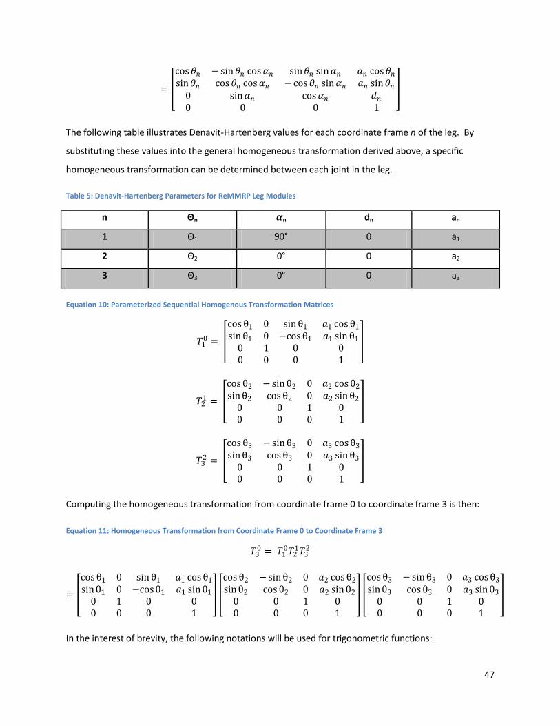
47
= �
cos𝜃𝜃𝑖𝑖 − sin𝜃𝜃𝑖𝑖 cos𝛼𝛼𝑖𝑖 sin𝜃𝜃𝑖𝑖 sin𝛼𝛼𝑖𝑖 𝑏𝑏𝑖𝑖 cos𝜃𝜃𝑖𝑖sin𝜃𝜃𝑖𝑖 cos𝜃𝜃𝑖𝑖 cos𝛼𝛼𝑖𝑖 − cos𝜃𝜃𝑖𝑖 sin𝛼𝛼𝑖𝑖 𝑏𝑏𝑖𝑖 sin𝜃𝜃𝑖𝑖
0 sin𝛼𝛼𝑖𝑖 cos𝛼𝛼𝑖𝑖 𝑑𝑑𝑖𝑖0 0 0 1
�
The following table illustrates Denavit-Hartenberg values for each coordinate frame n of the leg. By
substituting these values into the general homogeneous transformation derived above, a specific
homogeneous transformation can be determined between each joint in the leg.
Table 5: Denavit-Hartenberg Parameters for ReMMRP Leg Modules
n Θn 𝜶𝜶n dn an
1 Θ1 90° 0 a1
2 Θ2 0° 0 a2
3 Θ3 0° 0 a3
Equation 10: Parameterized Sequential Homogenous Transformation Matrices
𝑇𝑇10 = �
cosθ1 0 sinθ1 𝑏𝑏1 cosθ1sinθ1 0 −cosθ1 𝑏𝑏1 sinθ1
0 1 0 00 0 0 1
�
𝑇𝑇21 = �
cosθ2 − sinθ2 0 𝑏𝑏2 cosθ2sinθ2 cosθ2 0 𝑏𝑏2 sinθ2
0 0 1 00 0 0 1
�
𝑇𝑇32 = �
cosθ3 − sinθ3 0 𝑏𝑏3 cosθ3sinθ3 cosθ3 0 𝑏𝑏3 sinθ3
0 0 1 00 0 0 1
�
Computing the homogeneous transformation from coordinate frame 0 to coordinate frame 3 is then:
Equation 11: Homogeneous Transformation from Coordinate Frame 0 to Coordinate Frame 3
𝑇𝑇30 = 𝑇𝑇1
0𝑇𝑇21𝑇𝑇3
2
= �
cosθ1 0 sinθ1 𝑏𝑏1 cosθ1sinθ1 0 −cosθ1 𝑏𝑏1 sinθ1
0 1 0 00 0 0 1
� �
cosθ2 − sinθ2 0 𝑏𝑏2 cosθ2sinθ2 cosθ2 0 𝑏𝑏2 sinθ2
0 0 1 00 0 0 1
� �
cosθ3 − sinθ3 0 𝑏𝑏3 cosθ3sinθ3 cosθ3 0 𝑏𝑏3 sinθ3
0 0 1 00 0 0 1
�
In the interest of brevity, the following notations will be used for trigonometric functions:
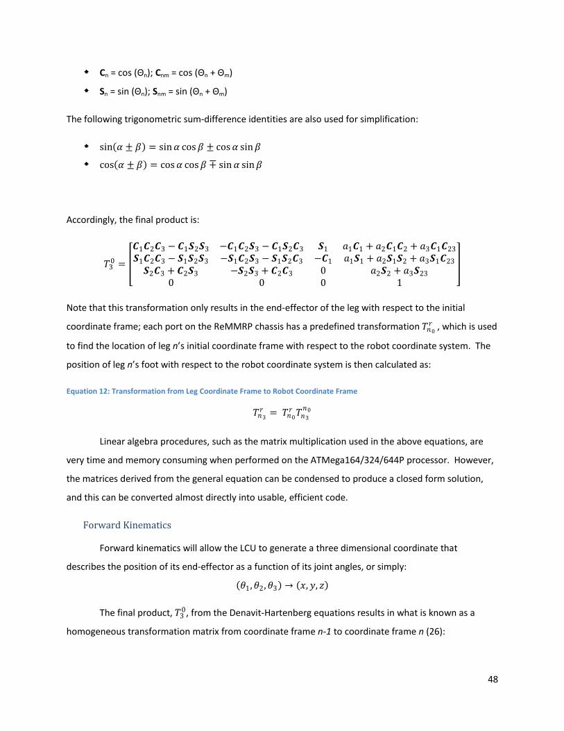
48
Cn = cos (Θn); Cnm = cos (Θn + Θm)
Sn = sin (Θn); Snm = sin (Θn + Θm)
The following trigonometric sum-difference identities are also used for simplification:
sin(𝛼𝛼 ± 𝛽𝛽) = sin𝛼𝛼 cos𝛽𝛽 ± cos𝛼𝛼 sin𝛽𝛽
cos(𝛼𝛼 ± 𝛽𝛽) = cos𝛼𝛼 cos𝛽𝛽 ∓ sin𝛼𝛼 sin𝛽𝛽
Accordingly, the final product is:
𝑇𝑇30 = �
𝑪𝑪1𝑪𝑪2𝑪𝑪3 − 𝑪𝑪1𝑺𝑺2𝑺𝑺3 −𝑪𝑪1𝑪𝑪2𝑺𝑺3 − 𝑪𝑪1𝑺𝑺2𝑪𝑪3 𝑺𝑺1 𝑏𝑏1𝑪𝑪1 + 𝑏𝑏2𝑪𝑪1𝑪𝑪2 + 𝑏𝑏3𝑪𝑪1𝑪𝑪23𝑺𝑺1𝑪𝑪2𝑪𝑪3 − 𝑺𝑺1𝑺𝑺2𝑺𝑺3 −𝑺𝑺1𝑪𝑪2𝑺𝑺3 − 𝑺𝑺1𝑺𝑺2𝑪𝑪3 −𝑪𝑪1 𝑏𝑏1𝑺𝑺1 + 𝑏𝑏2𝑺𝑺1𝑺𝑺2 + 𝑏𝑏3𝑺𝑺1𝑪𝑪23𝑺𝑺2𝑪𝑪3 + 𝑪𝑪2𝑺𝑺3 −𝑺𝑺2𝑺𝑺3 + 𝑪𝑪2𝑪𝑪3 0 𝑏𝑏2𝑺𝑺2 + 𝑏𝑏3𝑺𝑺23
0 0 0 1
�
Note that this transformation only results in the end-effector of the leg with respect to the initial
coordinate frame; each port on the ReMMRP chassis has a predefined transformation 𝑇𝑇𝑖𝑖0𝑏𝑏 , which is used
to find the location of leg n’s initial coordinate frame with respect to the robot coordinate system. The
position of leg n’s foot with respect to the robot coordinate system is then calculated as:
Equation 12: Transformation from Leg Coordinate Frame to Robot Coordinate Frame
𝑇𝑇𝑖𝑖3𝑏𝑏 = 𝑇𝑇𝑖𝑖0
𝑏𝑏 𝑇𝑇𝑖𝑖3𝑖𝑖0
Linear algebra procedures, such as the matrix multiplication used in the above equations, are
very time and memory consuming when performed on the ATMega164/324/644P processor. However,
the matrices derived from the general equation can be condensed to produce a closed form solution,
and this can be converted almost directly into usable, efficient code.
Forward Kinematics
Forward kinematics will allow the LCU to generate a three dimensional coordinate that
describes the position of its end-effector as a function of its joint angles, or simply:
(𝜃𝜃1,𝜃𝜃2,𝜃𝜃3) → (𝑥𝑥,𝑏𝑏, 𝑜𝑜)
The final product, 𝑇𝑇30, from the Denavit-Hartenberg equations results in what is known as a
homogeneous transformation matrix from coordinate frame n-1 to coordinate frame n (26):
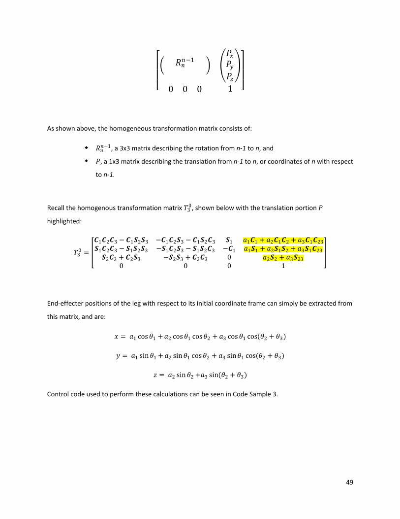
49
⎣⎢⎢⎡�
𝑅𝑅𝑖𝑖𝑖𝑖−1
� �𝑃𝑃𝑥𝑥𝑃𝑃𝑏𝑏𝑃𝑃𝑜𝑜�
0 0 0 1 ⎦⎥⎥⎤
As shown above, the homogeneous transformation matrix consists of:
𝑅𝑅𝑖𝑖𝑖𝑖−1, a 3x3 matrix describing the rotation from n-1 to n, and
𝑃𝑃, a 1x3 matrix describing the translation from n-1 to n, or coordinates of n with respect
to n-1.
Recall the homogenous transformation matrix 𝑇𝑇30, shown below with the translation portion 𝑃𝑃
highlighted:
𝑇𝑇30 = �
𝑪𝑪1𝑪𝑪2𝑪𝑪3 − 𝑪𝑪1𝑺𝑺2𝑺𝑺3 −𝑪𝑪1𝑪𝑪2𝑺𝑺3 − 𝑪𝑪1𝑺𝑺2𝑪𝑪3 𝑺𝑺1 𝑏𝑏1𝑪𝑪1 + 𝑏𝑏2𝑪𝑪1𝑪𝑪2 + 𝑏𝑏3𝑪𝑪1𝑪𝑪23𝑺𝑺1𝑪𝑪2𝑪𝑪3 − 𝑺𝑺1𝑺𝑺2𝑺𝑺3 −𝑺𝑺1𝑪𝑪2𝑺𝑺3 − 𝑺𝑺1𝑺𝑺2𝑪𝑪3 −𝑪𝑪1 𝑏𝑏1𝑺𝑺1 + 𝑏𝑏2𝑺𝑺1𝑺𝑺2 + 𝑏𝑏3𝑺𝑺1𝑪𝑪23𝑺𝑺2𝑪𝑪3 + 𝑪𝑪2𝑺𝑺3 −𝑺𝑺2𝑺𝑺3 + 𝑪𝑪2𝑪𝑪3 0 𝑏𝑏2𝑺𝑺2 + 𝑏𝑏3𝑺𝑺23
0 0 0 1
�
End-effecter positions of the leg with respect to its initial coordinate frame can simply be extracted from
this matrix, and are:
𝑥𝑥 = 𝑏𝑏1 cos𝜃𝜃1 +𝑏𝑏2 cos𝜃𝜃1 cos𝜃𝜃2 + 𝑏𝑏3 cos𝜃𝜃1 cos(𝜃𝜃2 + 𝜃𝜃3)
𝑏𝑏 = 𝑏𝑏1 sin𝜃𝜃1 +𝑏𝑏2 sin𝜃𝜃1 cos𝜃𝜃2 + 𝑏𝑏3 sin𝜃𝜃1 cos(𝜃𝜃2 + 𝜃𝜃3)
𝑜𝑜 = 𝑏𝑏2 sin𝜃𝜃2 +𝑏𝑏3 sin(𝜃𝜃2 + 𝜃𝜃3)
Control code used to perform these calculations can be seen in Code Sample 3.
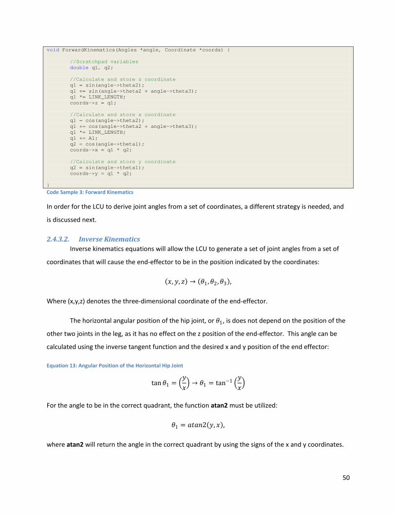
50
void ForwardKinematics(Angles *angle, Coordinate *coords) { //Scratchpad variables double q1, q2; //Calculate and store z coordinate q1 = sin(angle->theta2); q1 += sin(angle->theta2 + angle->theta3); q1 *= LINK_LENGTH; coords->z = q1; //Calculate and store x coordinate q1 = cos(angle->theta2); q1 += cos(angle->theta2 + angle->theta3); q1 *= LINK_LENGTH; q1 += A1; q2 = cos(angle->theta1); coords->x = q1 * q2; //Calculate and store y coordinate q2 = sin(angle->theta1); coords->y = q1 * q2; } Code Sample 3: Forward Kinematics
In order for the LCU to derive joint angles from a set of coordinates, a different strategy is needed, and
is discussed next.
2.4.3.2. Inverse Kinematics Inverse kinematics equations will allow the LCU to generate a set of joint angles from a set of
coordinates that will cause the end-effector to be in the position indicated by the coordinates:
(𝑥𝑥,𝑏𝑏, 𝑜𝑜) → (𝜃𝜃1,𝜃𝜃2,𝜃𝜃3),
Where (x,y,z) denotes the three-dimensional coordinate of the end-effector.
The horizontal angular position of the hip joint, or 𝜃𝜃1, is does not depend on the position of the
other two joints in the leg, as it has no effect on the z position of the end-effector. This angle can be
calculated using the inverse tangent function and the desired x and y position of the end effector:
Equation 13: Angular Position of the Horizontal Hip Joint
tan𝜃𝜃1 = �𝑏𝑏𝑥𝑥� → 𝜃𝜃1 = tan−1 �
𝑏𝑏𝑥𝑥�
For the angle to be in the correct quadrant, the function atan2 must be utilized:
𝜃𝜃1 = 𝑏𝑏𝑜𝑜𝑏𝑏𝑖𝑖2(𝑏𝑏, 𝑥𝑥),
where atan2 will return the angle in the correct quadrant by using the signs of the x and y coordinates.
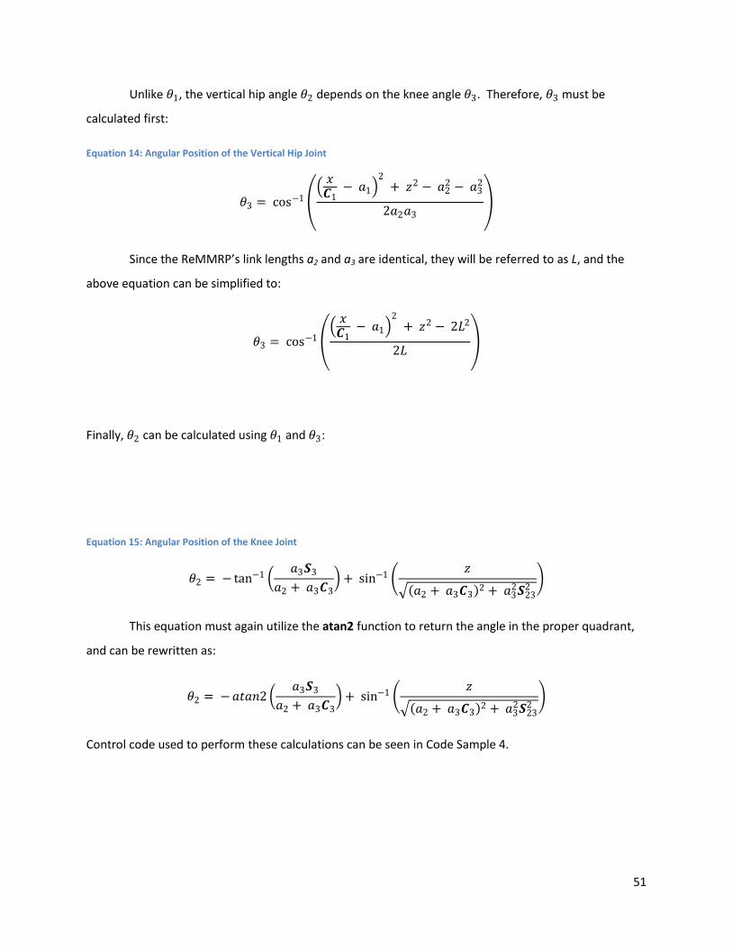
51
Unlike 𝜃𝜃1, the vertical hip angle 𝜃𝜃2 depends on the knee angle 𝜃𝜃3. Therefore, 𝜃𝜃3 must be
calculated first:
Equation 14: Angular Position of the Vertical Hip Joint
𝜃𝜃3 = cos−1 �� 𝑥𝑥𝑪𝑪1
− 𝑏𝑏1�2
+ 𝑜𝑜2 − 𝑏𝑏22 − 𝑏𝑏3
2
2𝑏𝑏2𝑏𝑏3�
Since the ReMMRP’s link lengths a2 and a3 are identical, they will be referred to as L, and the
above equation can be simplified to:
𝜃𝜃3 = cos−1 �� 𝑥𝑥𝑪𝑪1
− 𝑏𝑏1�2
+ 𝑜𝑜2 − 2𝐿𝐿2
2𝐿𝐿 �
Finally, 𝜃𝜃2 can be calculated using 𝜃𝜃1 and 𝜃𝜃3:
Equation 15: Angular Position of the Knee Joint
𝜃𝜃2 = − tan−1 �𝑏𝑏3𝑺𝑺3
𝑏𝑏2 + 𝑏𝑏3𝑪𝑪3� + sin−1 �
𝑜𝑜
�(𝑏𝑏2 + 𝑏𝑏3𝑪𝑪3)2 + 𝑏𝑏32𝑺𝑺23
2�
This equation must again utilize the atan2 function to return the angle in the proper quadrant,
and can be rewritten as:
𝜃𝜃2 = −𝑏𝑏𝑜𝑜𝑏𝑏𝑖𝑖2 �𝑏𝑏3𝑺𝑺3
𝑏𝑏2 + 𝑏𝑏3𝑪𝑪3�+ sin−1 �
𝑜𝑜
�(𝑏𝑏2 + 𝑏𝑏3𝑪𝑪3)2 + 𝑏𝑏32𝑺𝑺23
2�
Control code used to perform these calculations can be seen in Code Sample 4.
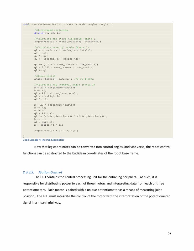
52
void InverseKinematics(Coordinate *coords, Angles *angle) { //Scratchpad variables double q1, q2, b; //Calculate and store hip angle (theta 1) angle->theta1 = atan2(coords->y, coords->x); //Calculate knee (y) angle (theta 3) q2 = (coords->x / cos(angle->theta1)); q2 -= A1; q2 *= q2; q2 += (coords->z * coords->z); q2 -= (2.000 * LINK_LENGTH * LINK_LENGTH); q1 = 2.000 * LINK_LENGTH * LINK_LENGTH; q2 /= q1; //Store theta3 angle->theta3 = acos(q2); //2-26 4:38pm //Calculate hip vertical angle (theta 2) b = A3 * cos(angle->theta3); b += A2; q1 = A3 * sin(angle->theta3); q2 = atan2(q1, b); q2 *= -1; b = A3 * cos(angle->theta3); b += A2; b *= b; q1 = A3 * A3; q1 *= (sin(angle->theta3) * sin(angle->theta3)); b += q1; q1 = sqrt(b); b = coords->z / q1; angle->theta2 = q2 + asin(b); } Code Sample 4: Inverse Kinematics
Now that leg coordinates can be converted into control angles, and vice versa, the robot control
functions can be abstracted to the Euclidean coordinates of the robot base frame.
2.4.3.3. Motion Control The LCU contains the central processing unit for the entire leg peripheral. As such, it is
responsible for distributing power to each of three motors and interpreting data from each of three
potentiometers. Each motor is paired with a unique potentiometer as a means of measuring joint
position. The LCU must integrate the control of the motor with the interpretation of the potentiometer
signal in a meaningful way.
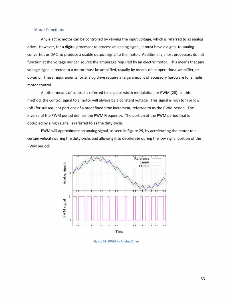
53
Motor Functions
Any electric motor can be controlled by varying the input voltage, which is referred to as analog
drive. However, for a digital processor to process an analog signal, it must have a digital-to-analog
converter, or DAC, to produce a usable output signal to the motor. Additionally, most processors do not
function at the voltage nor can source the amperage required by an electric motor. This means that any
voltage signal directed to a motor must be amplified, usually by means of an operational amplifier, or
op-amp. These requirements for analog drive require a large amount of accessory hardware for simple
motor control.
Another means of control is referred to as pulse width modulation, or PWM (28). In this
method, the control signal to a motor will always be a constant voltage. This signal is high (on) or low
(off) for subsequent portions of a predefined time increment, referred to as the PWM period. The
inverse of the PWM period defines the PWM Frequency. The portion of the PWM period that is
occupied by a high signal is referred to as the duty cycle.
PWM will approximate an analog signal, as seen in Figure 29, by accelerating the motor to a
certain velocity during the duty cycle, and allowing it to decelerate during the low signal portion of the
PWM period:
Figure 29: PWM vs Analog Drive
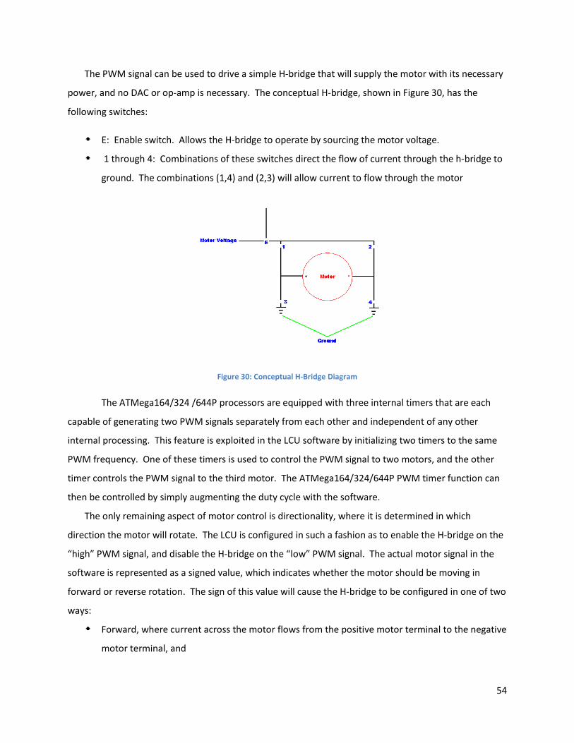
54
The PWM signal can be used to drive a simple H-bridge that will supply the motor with its necessary
power, and no DAC or op-amp is necessary. The conceptual H-bridge, shown in Figure 30, has the
following switches:
E: Enable switch. Allows the H-bridge to operate by sourcing the motor voltage.
1 through 4: Combinations of these switches direct the flow of current through the h-bridge to
ground. The combinations (1,4) and (2,3) will allow current to flow through the motor
Figure 30: Conceptual H-Bridge Diagram
The ATMega164/324 /644P processors are equipped with three internal timers that are each
capable of generating two PWM signals separately from each other and independent of any other
internal processing. This feature is exploited in the LCU software by initializing two timers to the same
PWM frequency. One of these timers is used to control the PWM signal to two motors, and the other
timer controls the PWM signal to the third motor. The ATMega164/324/644P PWM timer function can
then be controlled by simply augmenting the duty cycle with the software.
The only remaining aspect of motor control is directionality, where it is determined in which
direction the motor will rotate. The LCU is configured in such a fashion as to enable the H-bridge on the
“high” PWM signal, and disable the H-bridge on the “low” PWM signal. The actual motor signal in the
software is represented as a signed value, which indicates whether the motor should be moving in
forward or reverse rotation. The sign of this value will cause the H-bridge to be configured in one of two
ways:
Forward, where current across the motor flows from the positive motor terminal to the negative
motor terminal, and
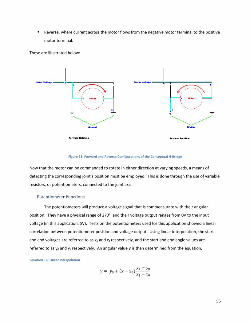
55
Reverse, where current across the motor flows from the negative motor terminal to the positive
motor terminal.
These are illustrated below:
Figure 31: Forward and Reverse Configurations of the Conceptual H-Bridge
Now that the motor can be commanded to rotate in either direction at varying speeds, a means of
detecting the corresponding joint’s position must be employed. This is done through the use of variable
resistors, or potentiometers, connected to the joint axis.
Potentiometer Functions
The potentiometers will produce a voltage signal that is commensurate with their angular
position. They have a physical range of 270°, and their voltage output ranges from 0V to the input
voltage (in this application, 5V). Tests on the potentiometers used for this application showed a linear
correlation between potentiometer position and voltage output. Using linear interpolation, the start
and end voltages are referred to as x0 and x1 respectively, and the start and end angle values are
referred to as y0 and y1 respectively. An angular value y is then determined from the equation,
Equation 16: Linear Interpolation
𝑏𝑏 = 𝑏𝑏0 + (𝑥𝑥 − 𝑥𝑥0)𝑏𝑏1 − 𝑏𝑏0
𝑥𝑥1 − 𝑥𝑥0

56
This still renders an analog voltage; the resulting value must be converted into one that can be used by
the ATMega164/324/644P processor.
The ATMega164/324/644P processors have a built-in analog to digital converter, or ADC. The
ADC functions by approximating a voltage input to a certain resolution; on the ATMega164/324/644P
this resolution is 10 bits. The input voltage is converted into a digital value in the range of 0 to
(2resolution)-1, or 0 to 1023.
The same linear interpolation can be used by replacing the voltage range of 0V to 5V with the
digital range of 0 to 1023.
2.4.3.4. PID Control In order to control the motor to arrive and stay at a given angle, a continuous means of control
must be implemented. Simply running the motor until it reaches a certain point will not work, since the
inertia of the motor and leg will continue to carry the axis past the desired point after the motor is shut
off. A controller must be used that monitors the relationship between the desired joint position and the
actual joint position, the difference in which is referred to as the error, and adjusts the motor’s behavior
to minimize the error.
Proportional-Integral-Derivative (PID) control uses the summation of three terms to monitor and
control the signal to a motor (29):
1. Proportional Term: the difference between the current motor position and the desired position.
Greater errors will cause a larger control signal to the motor. Proportional control alone is
typically subject to oscillations in the motor output.
2. Integral Term: the sum of the positional errors over time. The role of the integral term is to
decrease the oscillation caused by the Proportional control. By using the Integral control the
arm will eventually settle into the desired position.
3. Derivative Control: the rate of change in the error, used to balance the Integral control by
dampening the decaying oscillations from proportional-integral control.
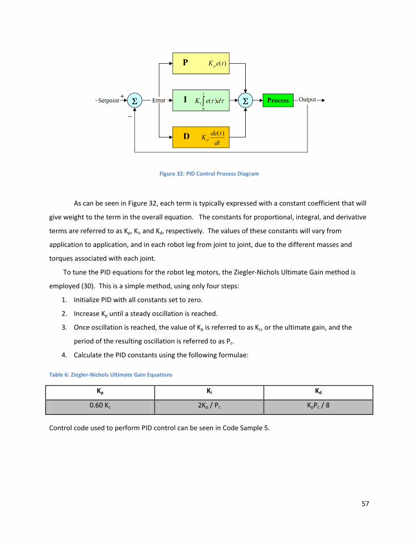
57
Figure 32: PID Control Process Diagram
As can be seen in Figure 32, each term is typically expressed with a constant coefficient that will
give weight to the term in the overall equation. The constants for proportional, integral, and derivative
terms are referred to as Kp, Ki, and Kd, respectively. The values of these constants will vary from
application to application, and in each robot leg from joint to joint, due to the different masses and
torques associated with each joint.
To tune the PID equations for the robot leg motors, the Ziegler-Nichols Ultimate Gain method is
employed (30). This is a simple method, using only four steps:
1. Initialize PID with all constants set to zero.
2. Increase Kp until a steady oscillation is reached.
3. Once oscillation is reached, the value of Kp is referred to as Kc, or the ultimate gain, and the
period of the resulting oscillation is referred to as Pc.
4. Calculate the PID constants using the following formulae:
Table 6: Ziegler-Nichols Ultimate Gain Equations
Kp Ki Kd
0.60 Kc 2Kp / Pc KpPc / 8
Control code used to perform PID control can be seen in Code Sample 5.
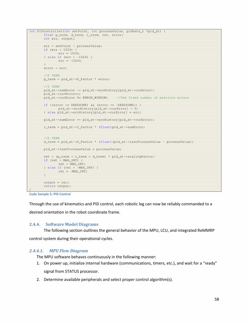
58
int PIDController(int setPoint, int processValue, pidData_t *pid_st) { float p_term, d_term, i_term, ret, error; int err, output; err = setPoint - processValue; if (err > 1024) { err = 1024; } else if (err < -1024) { err = -1024; } error = err; //P TERM p_term = pid_st->P_Factor * error; //I TERM pid_st->sumError -= pid_st->errHistory[pid_st->curError]; pid_st->curError++; pid_st->curError %= ERROR_WINDOW; //Use fixed number of previous errors if ((error <= DEADZONE) && (error >= -DEADZONE)) { pid_st->errHistory[pid_st->curError] = 0; } else pid_st->errHistory[pid_st->curError] = err; pid_st->sumError += pid_st->errHistory[pid_st->curError]; i_term = pid_st->I_Factor * (float)pid_st->sumError; //D TERM d_term = pid_st->D_Factor * (float)(pid_st->lastProcessValue - processValue); pid_st->lastProcessValue = processValue; ret = (p_term + i_term + d_term) * pid_st->scalingFactor; if (ret > MAX_INT) { ret = MAX_INT; } else if (ret < -MAX_INT) { ret = -MAX_INT; } output = ret; return output; } Code Sample 5: PID Control
Through the use of kinematics and PID control, each robotic leg can now be reliably commanded to a
desired orientation in the robot coordinate frame.
2.4.4. Software Model Diagrams The following section outlines the general behavior of the MPU, LCU, and integrated ReMMRP
control system during their operational cycles.
2.4.4.1. MPU Flow Diagram The MPU software behaves continuously in the following manner: 1. On power up, initialize internal hardware (communications, timers, etc.), and wait for a “ready”
signal from STATUS processor.
2. Determine available peripherals and select proper control algorithm(s).
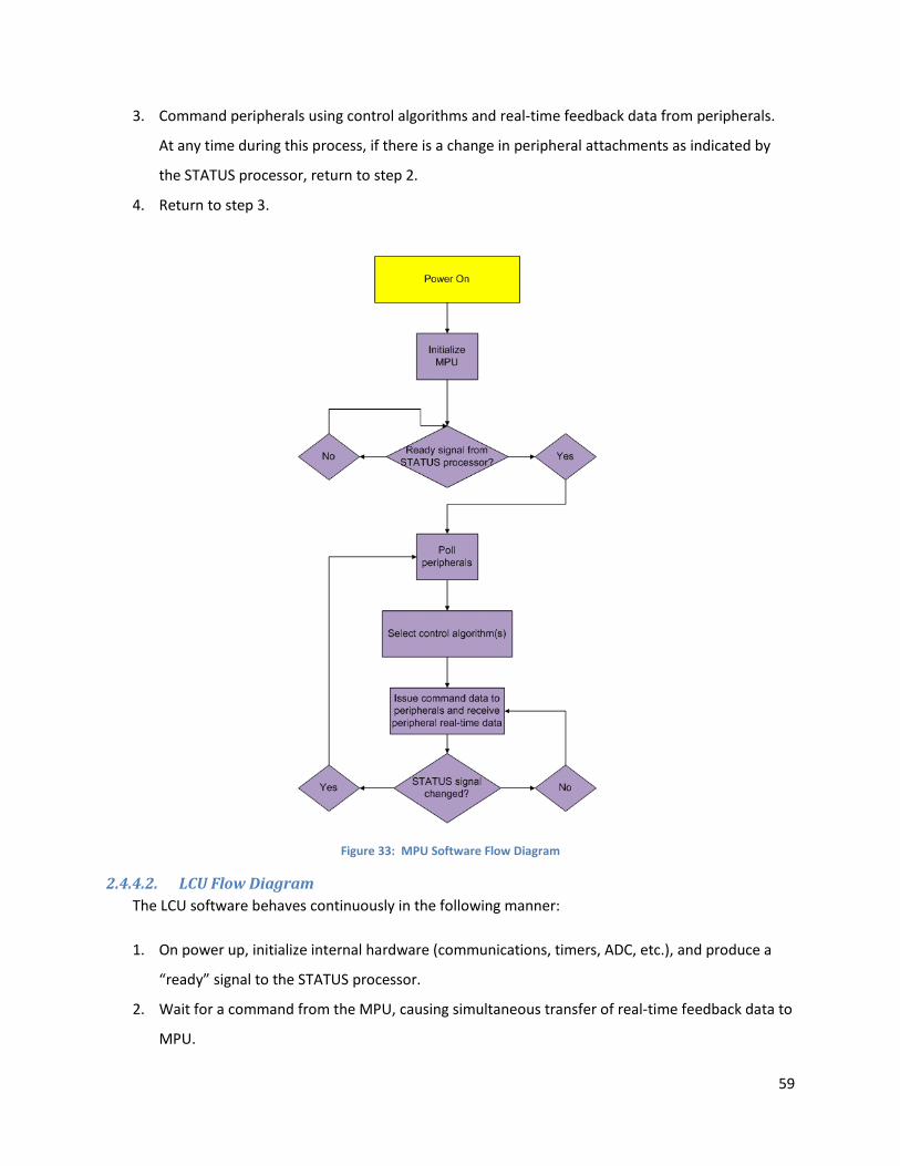
59
3. Command peripherals using control algorithms and real-time feedback data from peripherals.
At any time during this process, if there is a change in peripheral attachments as indicated by
the STATUS processor, return to step 2.
4. Return to step 3.
Figure 33: MPU Software Flow Diagram
2.4.4.2. LCU Flow Diagram The LCU software behaves continuously in the following manner:
1. On power up, initialize internal hardware (communications, timers, ADC, etc.), and produce a
“ready” signal to the STATUS processor.
2. Wait for a command from the MPU, causing simultaneous transfer of real-time feedback data to
MPU.
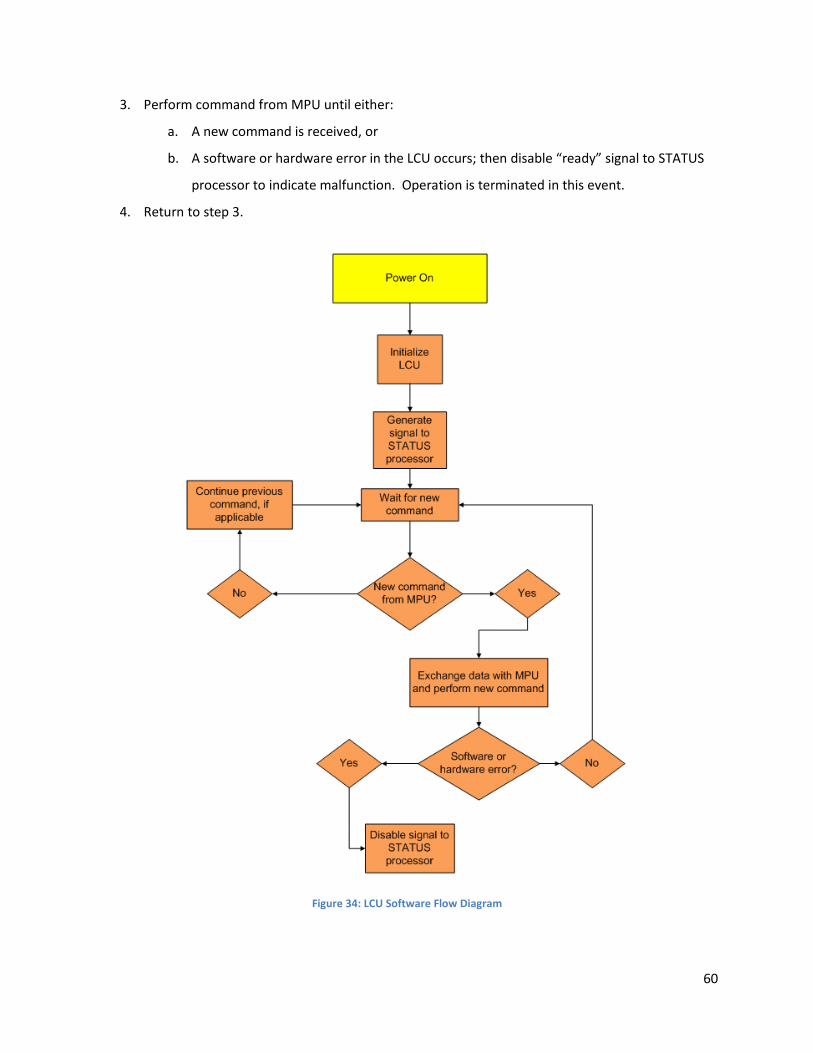
60
3. Perform command from MPU until either:
a. A new command is received, or
b. A software or hardware error in the LCU occurs; then disable “ready” signal to STATUS
processor to indicate malfunction. Operation is terminated in this event.
4. Return to step 3.
Figure 34: LCU Software Flow Diagram
61
2.4.4.3. Integrated Flow Diagram The complete software model of the robot behaves continuously in the following manner:
1. On power up, MPU, LCUs, and STATUS processors initialize.
2. LCUs (and other peripherals) send “ready” signal to the STATUS processor.
3. STATUS processor determines which ports have attached peripherals, or active ports, and
communicates this information to the MPU.
4. MPU polls active ports for identification information and creates a list of peripheral devices
based on type.
5. MPU groups similar peripherals and selects control algorithm to employ accordingly.
6. MPU utilizes control algorithm(s) to generate command data for peripherals.
7. Command data is distributed to peripherals while real-time configuration data is simultaneously
returned to the MPU.
8. Real-time peripheral configuration data is fed into the control algorithm(s) on the MPU to
generate new command data for the peripheral devices.
9. In the event of a change in peripherals, go to step 3.
10. Return to step 5.
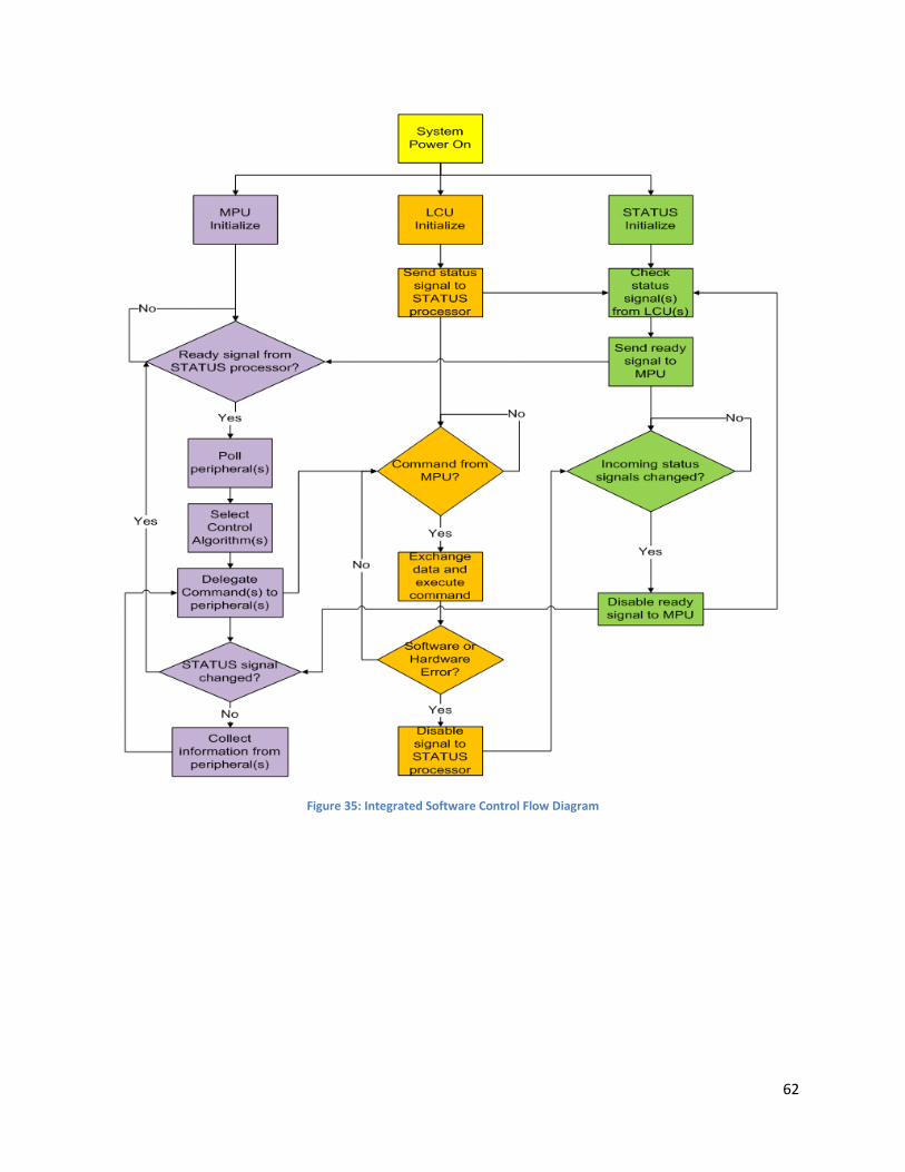
62
Figure 35: Integrated Software Control Flow Diagram
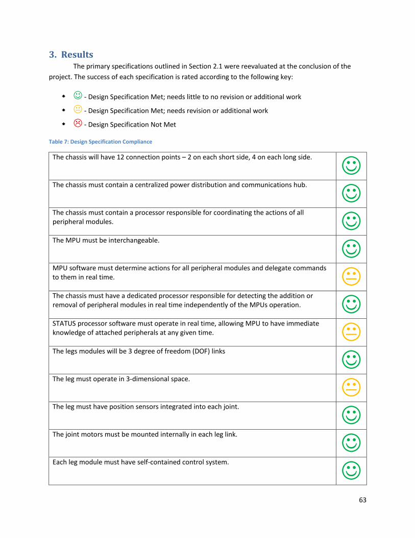
63
3. Results The primary specifications outlined in Section 2.1 were reevaluated at the conclusion of the
project. The success of each specification is rated according to the following key:
- Design Specification Met; needs little to no revision or additional work
- Design Specification Met; needs revision or additional work
- Design Specification Not Met
Table 7: Design Specification Compliance
The chassis will have 12 connection points – 2 on each short side, 4 on each long side.
The chassis must contain a centralized power distribution and communications hub.
The chassis must contain a processor responsible for coordinating the actions of all peripheral modules.
The MPU must be interchangeable.
MPU software must determine actions for all peripheral modules and delegate commands to them in real time.
The chassis must have a dedicated processor responsible for detecting the addition or removal of peripheral modules in real time independently of the MPUs operation.
STATUS processor software must operate in real time, allowing MPU to have immediate knowledge of attached peripherals at any given time.
The legs modules will be 3 degree of freedom (DOF) links
The leg must operate in 3-dimensional space.
The leg must have position sensors integrated into each joint.
The joint motors must be mounted internally in each leg link.
Each leg module must have self-contained control system.
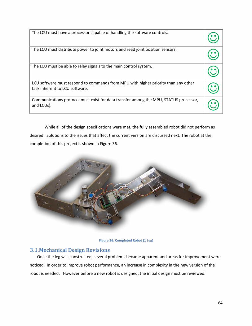
64
The LCU must have a processor capable of handling the software controls.
The LCU must distribute power to joint motors and read joint position sensors.
The LCU must be able to relay signals to the main control system.
LCU software must respond to commands from MPU with higher priority than any other task inherent to LCU software.
Communications protocol must exist for data transfer among the MPU, STATUS processor, and LCUs).
While all of the design specifications were met, the fully assembled robot did not perform as
desired. Solutions to the issues that affect the current version are discussed next. The robot at the
completion of this project is shown in Figure 36.
Figure 36: Completed Robot (1 Leg)
3.1. Mechanical Design Revisions Once the leg was constructed, several problems became apparent and areas for improvement were
noticed. In order to improve robot performance, an increase in complexity in the new version of the
robot is needed. However before a new robot is designed, the initial design must be reviewed.
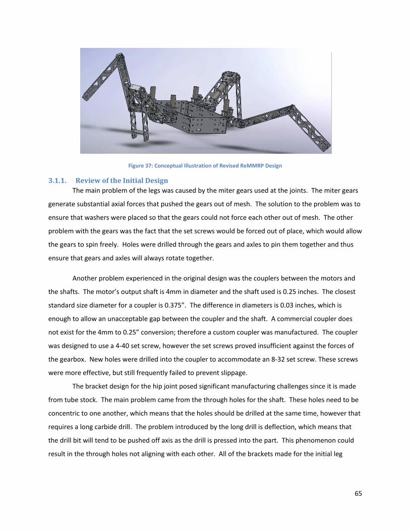
65
Figure 37: Conceptual Illustration of Revised ReMMRP Design
3.1.1. Review of the Initial Design The main problem of the legs was caused by the miter gears used at the joints. The miter gears
generate substantial axial forces that pushed the gears out of mesh. The solution to the problem was to
ensure that washers were placed so that the gears could not force each other out of mesh. The other
problem with the gears was the fact that the set screws would be forced out of place, which would allow
the gears to spin freely. Holes were drilled through the gears and axles to pin them together and thus
ensure that gears and axles will always rotate together.
Another problem experienced in the original design was the couplers between the motors and
the shafts. The motor’s output shaft is 4mm in diameter and the shaft used is 0.25 inches. The closest
standard size diameter for a coupler is 0.375”. The difference in diameters is 0.03 inches, which is
enough to allow an unacceptable gap between the coupler and the shaft. A commercial coupler does
not exist for the 4mm to 0.25” conversion; therefore a custom coupler was manufactured. The coupler
was designed to use a 4-40 set screw, however the set screws proved insufficient against the forces of
the gearbox. New holes were drilled into the coupler to accommodate an 8-32 set screw. These screws
were more effective, but still frequently failed to prevent slippage.
The bracket design for the hip joint posed significant manufacturing challenges since it is made
from tube stock. The main problem came from the through holes for the shaft. These holes need to be
concentric to one another, which means that the holes should be drilled at the same time, however that
requires a long carbide drill. The problem introduced by the long drill is deflection, which means that
the drill bit will tend to be pushed off axis as the drill is pressed into the part. This phenomenon could
result in the through holes not aligning with each other. All of the brackets made for the initial leg
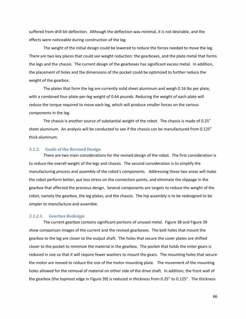
66
suffered from drill bit deflection. Although the deflection was minimal, it is not desirable, and the
effects were noticeable during construction of the leg.
The weight of the initial design could be lowered to reduce the forces needed to move the leg.
There are two key places that could see weight reduction: the gearboxes, and the plate metal that forms
the legs and the chassis. The current design of the gearboxes has significant excess metal. In addition,
the placement of holes and the dimensions of the pocket could be optimized to further reduce the
weight of the gearbox.
The plates that form the leg are currently solid sheet aluminum and weigh 0.16 lbs per plate,
with a combined four-plate-per-leg weight of 0.64 pounds. Reducing the weight of each plate will
reduce the torque required to move each leg, which will produce smaller forces on the various
components in the leg.
The chassis is another source of substantial weight of the robot. The chassis is made of 0.25”
sheet aluminum. An analysis will be conducted to see if the chassis can be manufactured from 0.125”
thick aluminum.
3.1.2. Goals of the Revised Design There are two main considerations for the revised design of the robot. The first consideration is
to reduce the overall weight of the legs and chassis. The second consideration is to simplify the
manufacturing process and assembly of the robot’s components. Addressing these two areas will make
the robot perform better, put less stress on the connection points, and eliminate the slippage in the
gearbox that affected the previous design. Several components are targets to reduce the weight of the
robot, namely the gearbox, the leg plates, and the chassis. The hip assembly is to be redesigned to be
simpler to manufacture and assemble.
3.1.2.1. Gearbox Redesign The current gearbox contains significant portions of unused metal. Figure 38 and Figure 39
show comparison images of the current and the revised gearboxes. The bolt holes that mount the
gearbox to the leg are closer to the output shaft. The holes that secure the cover plates are shifted
closer to the pocket to minimize the material in the gearbox. The pocket that holds the miter gears is
reduced in size so that it will require fewer washers to mount the gears. The mounting holes that secure
the motor are moved to reduce the size of the motor mounting plate. The movement of the mounting
holes allowed for the removal of material on either side of the drive shaft. In addition, the front wall of
the gearbox (the topmost edge in Figure 39) is reduced in thickness from 0.25” to 0.125”. The thickness
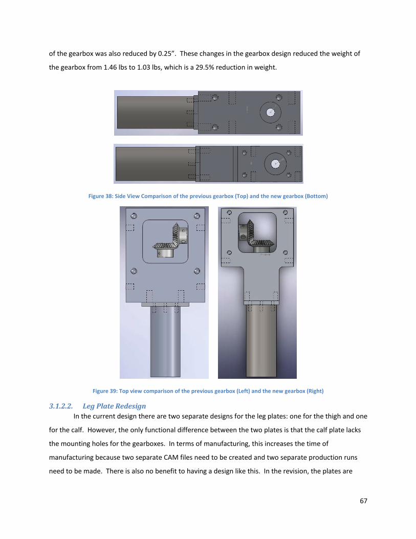
67
of the gearbox was also reduced by 0.25”. These changes in the gearbox design reduced the weight of
the gearbox from 1.46 lbs to 1.03 lbs, which is a 29.5% reduction in weight.
Figure 38: Side View Comparison of the previous gearbox (Top) and the new gearbox (Bottom)
Figure 39: Top view comparison of the previous gearbox (Left) and the new gearbox (Right)
3.1.2.2. Leg Plate Redesign In the current design there are two separate designs for the leg plates: one for the thigh and one
for the calf. However, the only functional difference between the two plates is that the calf plate lacks
the mounting holes for the gearboxes. In terms of manufacturing, this increases the time of
manufacturing because two separate CAM files need to be created and two separate production runs
need to be made. There is also no benefit to having a design like this. In the revision, the plates are
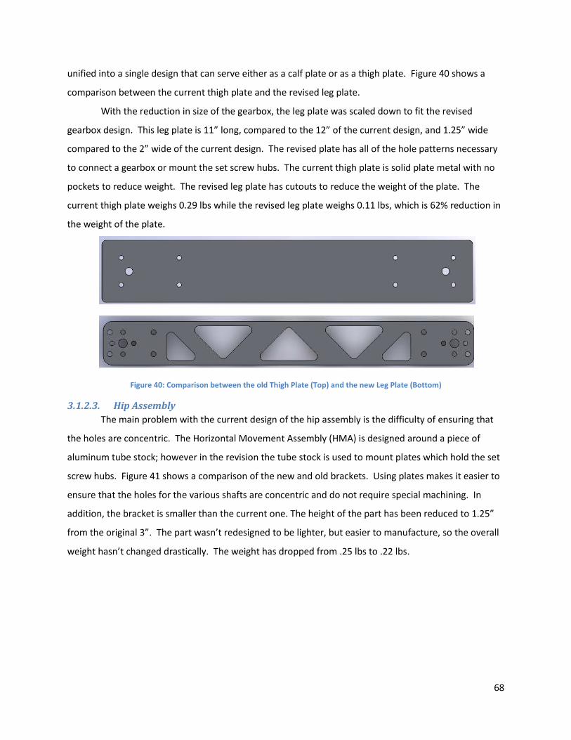
68
unified into a single design that can serve either as a calf plate or as a thigh plate. Figure 40 shows a
comparison between the current thigh plate and the revised leg plate.
With the reduction in size of the gearbox, the leg plate was scaled down to fit the revised
gearbox design. This leg plate is 11” long, compared to the 12” of the current design, and 1.25” wide
compared to the 2” wide of the current design. The revised plate has all of the hole patterns necessary
to connect a gearbox or mount the set screw hubs. The current thigh plate is solid plate metal with no
pockets to reduce weight. The revised leg plate has cutouts to reduce the weight of the plate. The
current thigh plate weighs 0.29 lbs while the revised leg plate weighs 0.11 lbs, which is 62% reduction in
the weight of the plate.
Figure 40: Comparison between the old Thigh Plate (Top) and the new Leg Plate (Bottom)
3.1.2.3. Hip Assembly The main problem with the current design of the hip assembly is the difficulty of ensuring that
the holes are concentric. The Horizontal Movement Assembly (HMA) is designed around a piece of
aluminum tube stock; however in the revision the tube stock is used to mount plates which hold the set
screw hubs. Figure 41 shows a comparison of the new and old brackets. Using plates makes it easier to
ensure that the holes for the various shafts are concentric and do not require special machining. In
addition, the bracket is smaller than the current one. The height of the part has been reduced to 1.25”
from the original 3”. The part wasn’t redesigned to be lighter, but easier to manufacture, so the overall
weight hasn’t changed drastically. The weight has dropped from .25 lbs to .22 lbs.
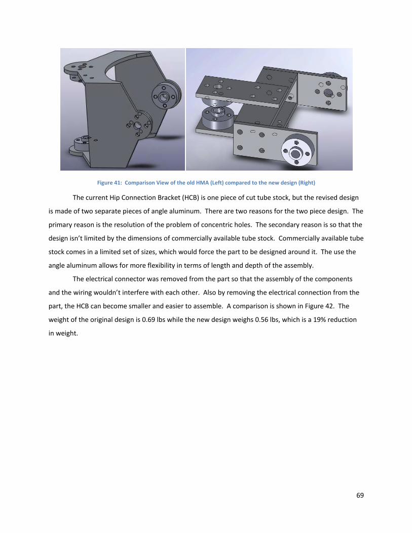
69
Figure 41: Comparison View of the old HMA (Left) compared to the new design (Right)
The current Hip Connection Bracket (HCB) is one piece of cut tube stock, but the revised design
is made of two separate pieces of angle aluminum. There are two reasons for the two piece design. The
primary reason is the resolution of the problem of concentric holes. The secondary reason is so that the
design isn’t limited by the dimensions of commercially available tube stock. Commercially available tube
stock comes in a limited set of sizes, which would force the part to be designed around it. The use the
angle aluminum allows for more flexibility in terms of length and depth of the assembly.
The electrical connector was removed from the part so that the assembly of the components
and the wiring wouldn’t interfere with each other. Also by removing the electrical connection from the
part, the HCB can become smaller and easier to assemble. A comparison is shown in Figure 42. The
weight of the original design is 0.69 lbs while the new design weighs 0.56 lbs, which is a 19% reduction
in weight.
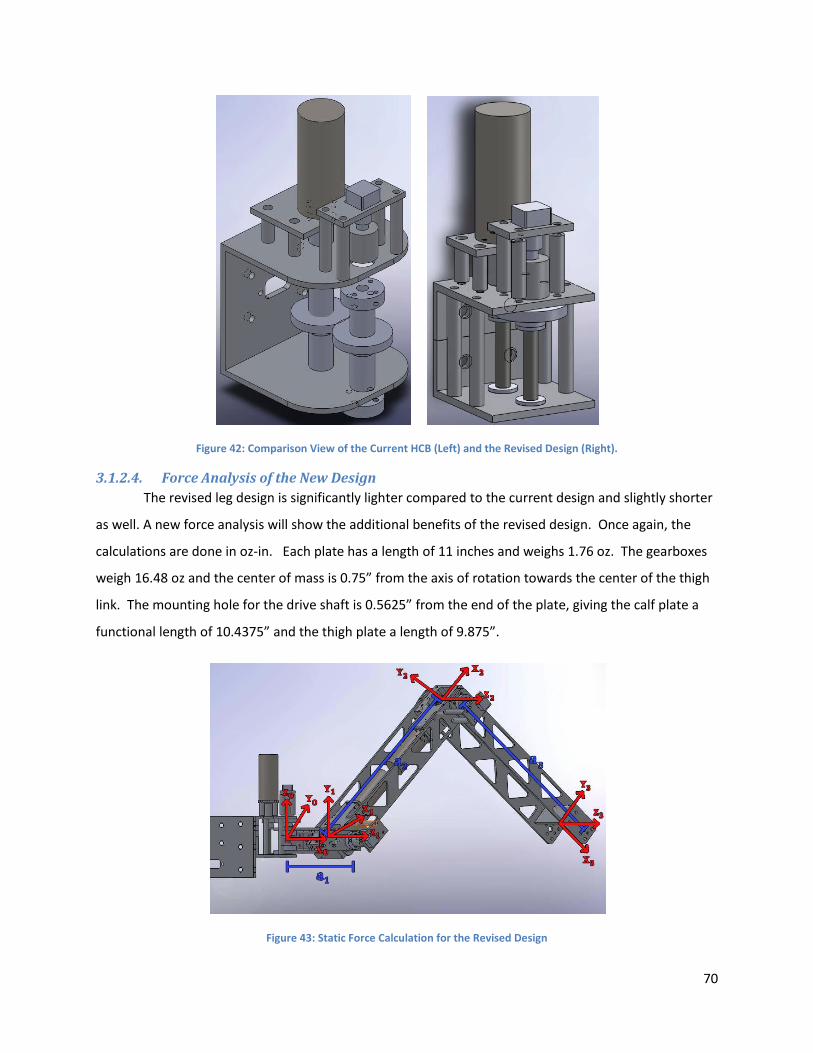
70
Figure 42: Comparison View of the Current HCB (Left) and the Revised Design (Right).
3.1.2.4. Force Analysis of the New Design The revised leg design is significantly lighter compared to the current design and slightly shorter
as well. A new force analysis will show the additional benefits of the revised design. Once again, the
calculations are done in oz-in. Each plate has a length of 11 inches and weighs 1.76 oz. The gearboxes
weigh 16.48 oz and the center of mass is 0.75” from the axis of rotation towards the center of the thigh
link. The mounting hole for the drive shaft is 0.5625” from the end of the plate, giving the calf plate a
functional length of 10.4375” and the thigh plate a length of 9.875”.
Figure 43: Static Force Calculation for the Revised Design
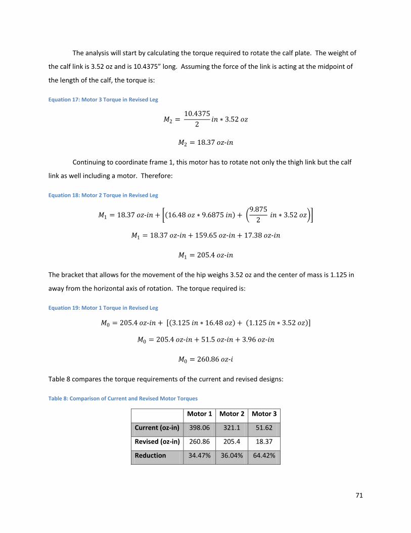
71
The analysis will start by calculating the torque required to rotate the calf plate. The weight of
the calf link is 3.52 oz and is 10.4375” long. Assuming the force of the link is acting at the midpoint of
the length of the calf, the torque is:
Equation 17: Motor 3 Torque in Revised Leg
𝑀𝑀2 = 10.4375
2𝑖𝑖𝑖𝑖 ∗ 3.52 𝑜𝑜𝑜𝑜
𝑀𝑀2 = 18.37 𝑜𝑜𝑜𝑜-𝑖𝑖𝑖𝑖
Continuing to coordinate frame 1, this motor has to rotate not only the thigh link but the calf
link as well including a motor. Therefore:
Equation 18: Motor 2 Torque in Revised Leg
𝑀𝑀1 = 18.37 𝑜𝑜𝑜𝑜-𝑖𝑖𝑖𝑖 + �(16.48 𝑜𝑜𝑜𝑜 ∗ 9.6875 𝑖𝑖𝑖𝑖) + �9.875
2 𝑖𝑖𝑖𝑖 ∗ 3.52 𝑜𝑜𝑜𝑜��
𝑀𝑀1 = 18.37 𝑜𝑜𝑜𝑜-𝑖𝑖𝑖𝑖 + 159.65 𝑜𝑜𝑜𝑜-𝑖𝑖𝑖𝑖 + 17.38 𝑜𝑜𝑜𝑜-𝑖𝑖𝑖𝑖
𝑀𝑀1 = 205.4 𝑜𝑜𝑜𝑜-𝑖𝑖𝑖𝑖
The bracket that allows for the movement of the hip weighs 3.52 oz and the center of mass is 1.125 in
away from the horizontal axis of rotation. The torque required is:
Equation 19: Motor 1 Torque in Revised Leg
𝑀𝑀0 = 205.4 𝑜𝑜𝑜𝑜-𝑖𝑖𝑖𝑖 + [(3.125 𝑖𝑖𝑖𝑖 ∗ 16.48 𝑜𝑜𝑜𝑜) + (1.125 𝑖𝑖𝑖𝑖 ∗ 3.52 𝑜𝑜𝑜𝑜)]
𝑀𝑀0 = 205.4 𝑜𝑜𝑜𝑜-𝑖𝑖𝑖𝑖 + 51.5 𝑜𝑜𝑜𝑜-𝑖𝑖𝑖𝑖 + 3.96 𝑜𝑜𝑜𝑜-𝑖𝑖𝑖𝑖
𝑀𝑀0 = 260.86 𝑜𝑜𝑜𝑜-𝑖𝑖
Table 8 compares the torque requirements of the current and revised designs:
Table 8: Comparison of Current and Revised Motor Torques
Motor 1 Motor 2 Motor 3
Current (oz-in) 398.06 321.1 51.62
Revised (oz-in) 260.86 205.4 18.37
Reduction 34.47% 36.04% 64.42%
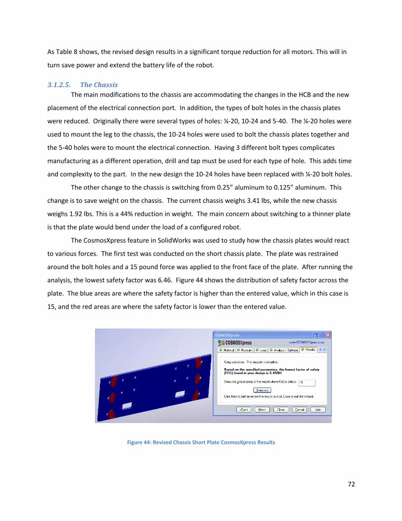
72
As Table 8 shows, the revised design results in a significant torque reduction for all motors. This will in
turn save power and extend the battery life of the robot.
3.1.2.5. The Chassis The main modifications to the chassis are accommodating the changes in the HCB and the new
placement of the electrical connection port. In addition, the types of bolt holes in the chassis plates
were reduced. Originally there were several types of holes: ¼-20, 10-24 and 5-40. The ¼-20 holes were
used to mount the leg to the chassis, the 10-24 holes were used to bolt the chassis plates together and
the 5-40 holes were to mount the electrical connection. Having 3 different bolt types complicates
manufacturing as a different operation, drill and tap must be used for each type of hole. This adds time
and complexity to the part. In the new design the 10-24 holes have been replaced with ¼-20 bolt holes.
The other change to the chassis is switching from 0.25” aluminum to 0.125” aluminum. This
change is to save weight on the chassis. The current chassis weighs 3.41 lbs, while the new chassis
weighs 1.92 lbs. This is a 44% reduction in weight. The main concern about switching to a thinner plate
is that the plate would bend under the load of a configured robot.
The CosmosXpress feature in SolidWorks was used to study how the chassis plates would react
to various forces. The first test was conducted on the short chassis plate. The plate was restrained
around the bolt holes and a 15 pound force was applied to the front face of the plate. After running the
analysis, the lowest safety factor was 6.46. Figure 44 shows the distribution of safety factor across the
plate. The blue areas are where the safety factor is higher than the entered value, which in this case is
15, and the red areas are where the safety factor is lower than the entered value.
Figure 44: Revised Chassis Short Plate CosmosXpress Results
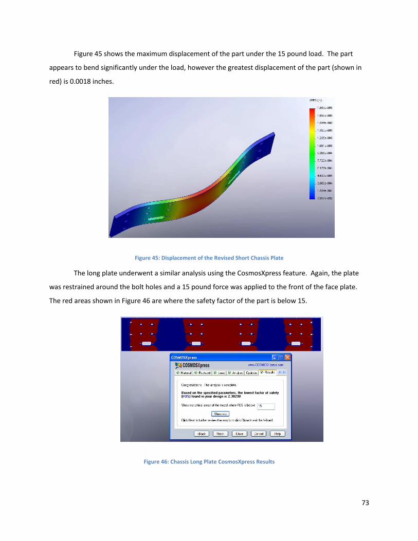
73
Figure 45 shows the maximum displacement of the part under the 15 pound load. The part
appears to bend significantly under the load, however the greatest displacement of the part (shown in
red) is 0.0018 inches.
Figure 45: Displacement of the Revised Short Chassis Plate
The long plate underwent a similar analysis using the CosmosXpress feature. Again, the plate
was restrained around the bolt holes and a 15 pound force was applied to the front of the face plate.
The red areas shown in Figure 46 are where the safety factor of the part is below 15.
Figure 46: Chassis Long Plate CosmosXpress Results
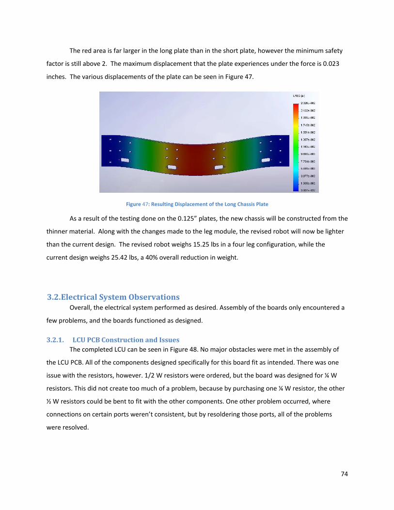
74
The red area is far larger in the long plate than in the short plate, however the minimum safety
factor is still above 2. The maximum displacement that the plate experiences under the force is 0.023
inches. The various displacements of the plate can be seen in Figure 47.
Figure 47: Resulting Displacement of the Long Chassis Plate
As a result of the testing done on the 0.125” plates, the new chassis will be constructed from the
thinner material. Along with the changes made to the leg module, the revised robot will now be lighter
than the current design. The revised robot weighs 15.25 lbs in a four leg configuration, while the
current design weighs 25.42 lbs, a 40% overall reduction in weight.
3.2. Electrical System Observations Overall, the electrical system performed as desired. Assembly of the boards only encountered a
few problems, and the boards functioned as designed.
3.2.1. LCU PCB Construction and Issues The completed LCU can be seen in Figure 48. No major obstacles were met in the assembly of
the LCU PCB. All of the components designed specifically for this board fit as intended. There was one
issue with the resistors, however. 1/2 W resistors were ordered, but the board was designed for ¼ W
resistors. This did not create too much of a problem, because by purchasing one ¼ W resistor, the other
½ W resistors could be bent to fit with the other components. One other problem occurred, where
connections on certain ports weren’t consistent, but by resoldering those ports, all of the problems
were resolved.
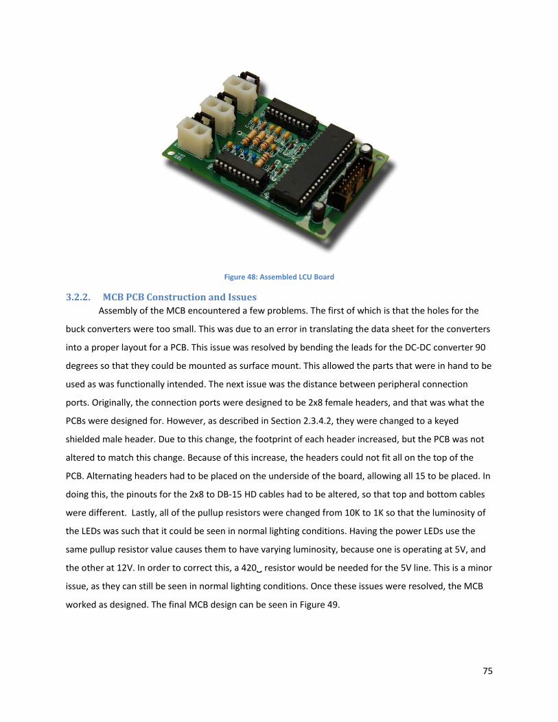
75
Figure 48: Assembled LCU Board
3.2.2. MCB PCB Construction and Issues Assembly of the MCB encountered a few problems. The first of which is that the holes for the
buck converters were too small. This was due to an error in translating the data sheet for the converters
into a proper layout for a PCB. This issue was resolved by bending the leads for the DC-DC converter 90
degrees so that they could be mounted as surface mount. This allowed the parts that were in hand to be
used as was functionally intended. The next issue was the distance between peripheral connection
ports. Originally, the connection ports were designed to be 2x8 female headers, and that was what the
PCBs were designed for. However, as described in Section 2.3.4.2, they were changed to a keyed
shielded male header. Due to this change, the footprint of each header increased, but the PCB was not
altered to match this change. Because of this increase, the headers could not fit all on the top of the
PCB. Alternating headers had to be placed on the underside of the board, allowing all 15 to be placed. In
doing this, the pinouts for the 2x8 to DB-15 HD cables had to be altered, so that top and bottom cables
were different. Lastly, all of the pullup resistors were changed from 10K to 1K so that the luminosity of
the LEDs was such that it could be seen in normal lighting conditions. Having the power LEDs use the
same pullup resistor value causes them to have varying luminosity, because one is operating at 5V, and
the other at 12V. In order to correct this, a 420 resistor would be needed for the 5V line. This is a minor
issue, as they can still be seen in normal lighting conditions. Once these issues were resolved, the MCB
worked as designed. The final MCB design can be seen in Figure 49.
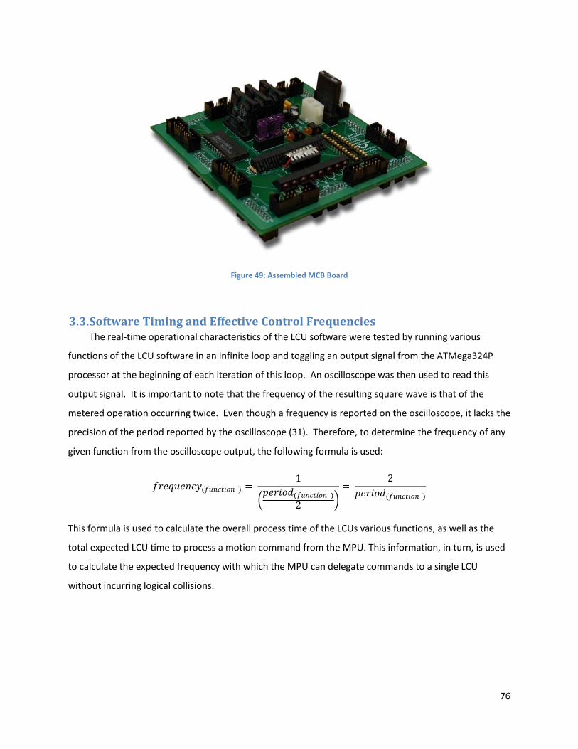
76
Figure 49: Assembled MCB Board
3.3. Software Timing and Effective Control Frequencies The real-time operational characteristics of the LCU software were tested by running various
functions of the LCU software in an infinite loop and toggling an output signal from the ATMega324P
processor at the beginning of each iteration of this loop. An oscilloscope was then used to read this
output signal. It is important to note that the frequency of the resulting square wave is that of the
metered operation occurring twice. Even though a frequency is reported on the oscilloscope, it lacks the
precision of the period reported by the oscilloscope (31). Therefore, to determine the frequency of any
given function from the oscilloscope output, the following formula is used:
𝑓𝑓𝑏𝑏𝑓𝑓𝑓𝑓𝑜𝑜𝑓𝑓𝑖𝑖𝑓𝑓𝑏𝑏(𝑓𝑓𝑜𝑜𝑖𝑖𝑓𝑓𝑜𝑜𝑖𝑖𝑜𝑜𝑖𝑖 ) = 1
�𝑜𝑜𝑓𝑓𝑏𝑏𝑖𝑖𝑜𝑜𝑑𝑑(𝑓𝑓𝑜𝑜𝑖𝑖𝑓𝑓𝑜𝑜𝑖𝑖𝑜𝑜𝑖𝑖 )
2 �=
2𝑜𝑜𝑓𝑓𝑏𝑏𝑖𝑖𝑜𝑜𝑑𝑑(𝑓𝑓𝑜𝑜𝑖𝑖𝑓𝑓𝑜𝑜𝑖𝑖𝑜𝑜𝑖𝑖 )
This formula is used to calculate the overall process time of the LCUs various functions, as well as the
total expected LCU time to process a motion command from the MPU. This information, in turn, is used
to calculate the expected frequency with which the MPU can delegate commands to a single LCU
without incurring logical collisions.
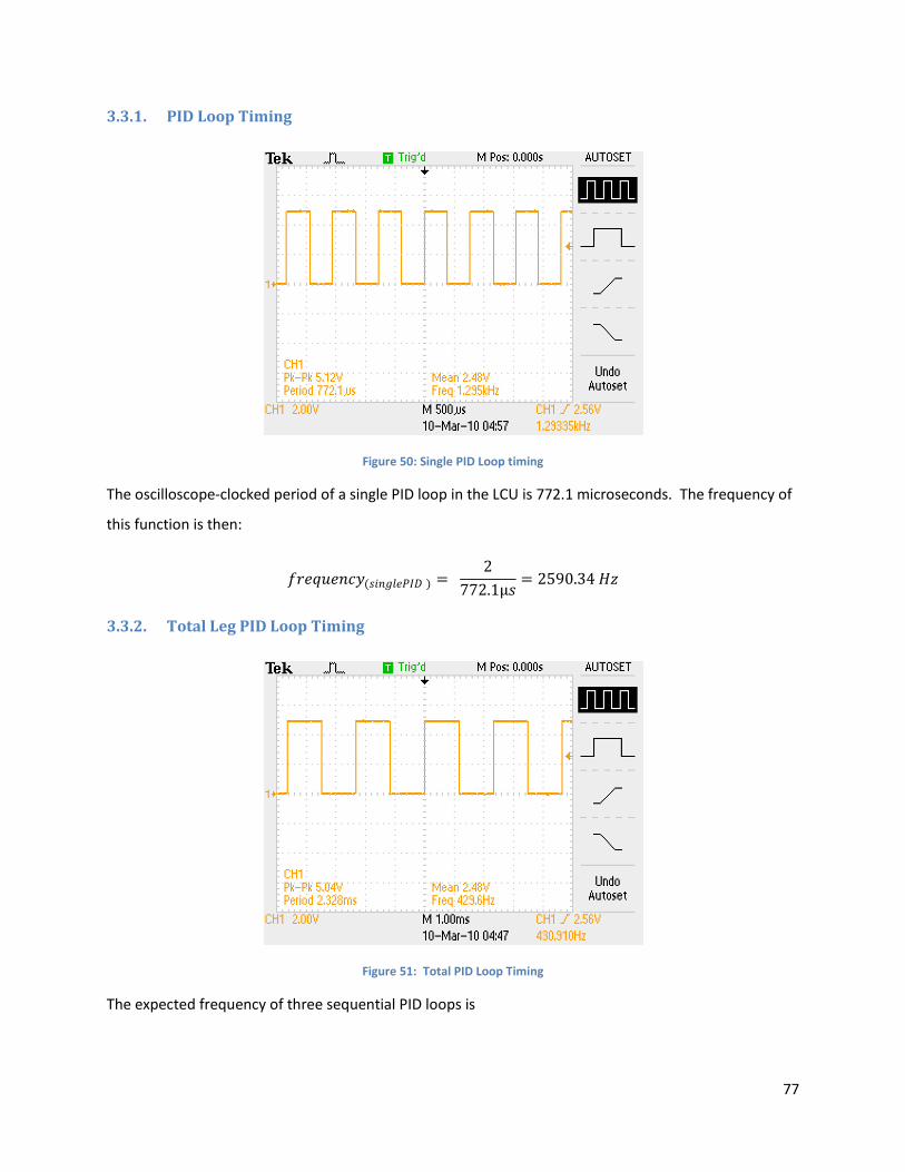
77
3.3.1. PID Loop Timing
Figure 50: Single PID Loop timing
The oscilloscope-clocked period of a single PID loop in the LCU is 772.1 microseconds. The frequency of
this function is then:
𝑓𝑓𝑏𝑏𝑓𝑓𝑓𝑓𝑜𝑜𝑓𝑓𝑖𝑖𝑓𝑓𝑏𝑏(𝑜𝑜𝑖𝑖𝑖𝑖𝑠𝑠𝑠𝑠𝑓𝑓𝑃𝑃𝑠𝑠𝑠𝑠 ) = 2
772.1µ𝑜𝑜= 2590.34 𝐻𝐻𝑜𝑜
3.3.2. Total Leg PID Loop Timing
Figure 51: Total PID Loop Timing
The expected frequency of three sequential PID loops is
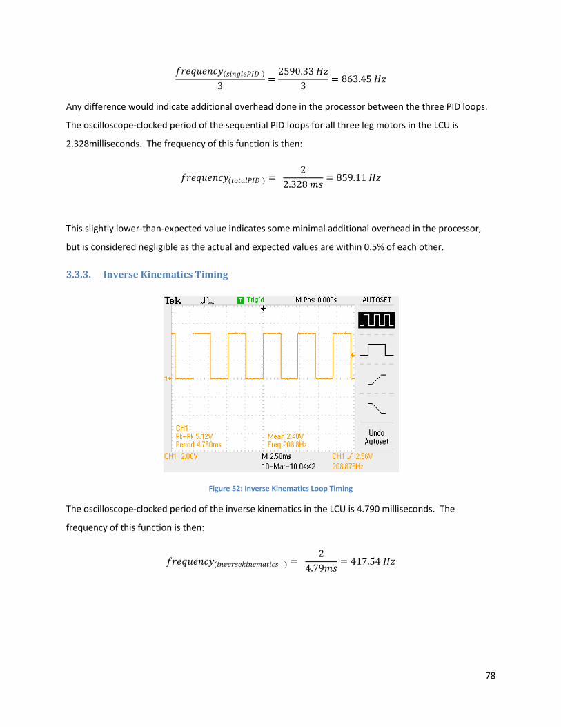
78
𝑓𝑓𝑏𝑏𝑓𝑓𝑓𝑓𝑜𝑜𝑓𝑓𝑖𝑖𝑓𝑓𝑏𝑏(𝑜𝑜𝑖𝑖𝑖𝑖𝑠𝑠𝑠𝑠𝑓𝑓𝑃𝑃𝑠𝑠𝑠𝑠 )
3=
2590.33 𝐻𝐻𝑜𝑜3
= 863.45 𝐻𝐻𝑜𝑜
Any difference would indicate additional overhead done in the processor between the three PID loops.
The oscilloscope-clocked period of the sequential PID loops for all three leg motors in the LCU is
2.328milliseconds. The frequency of this function is then:
𝑓𝑓𝑏𝑏𝑓𝑓𝑓𝑓𝑜𝑜𝑓𝑓𝑖𝑖𝑓𝑓𝑏𝑏(𝑜𝑜𝑜𝑜𝑜𝑜𝑏𝑏𝑠𝑠𝑃𝑃𝑠𝑠𝑠𝑠 ) = 2
2.328 𝑚𝑚𝑜𝑜= 859.11 𝐻𝐻𝑜𝑜
This slightly lower-than-expected value indicates some minimal additional overhead in the processor,
but is considered negligible as the actual and expected values are within 0.5% of each other.
3.3.3. Inverse Kinematics Timing
Figure 52: Inverse Kinematics Loop Timing
The oscilloscope-clocked period of the inverse kinematics in the LCU is 4.790 milliseconds. The
frequency of this function is then:
𝑓𝑓𝑏𝑏𝑓𝑓𝑓𝑓𝑜𝑜𝑓𝑓𝑖𝑖𝑓𝑓𝑏𝑏(𝑖𝑖𝑖𝑖𝑖𝑖𝑓𝑓𝑏𝑏𝑜𝑜𝑓𝑓𝑖𝑖𝑖𝑖𝑖𝑖𝑓𝑓𝑚𝑚𝑏𝑏𝑜𝑜𝑖𝑖𝑓𝑓𝑜𝑜 ) = 2
4.79𝑚𝑚𝑜𝑜= 417.54 𝐻𝐻𝑜𝑜
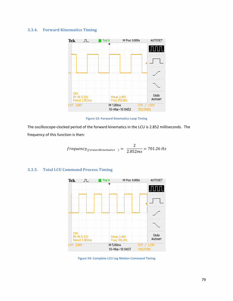
79
3.3.4. Forward Kinematics Timing
Figure 53: Forward Kinematics Loop Timing
The oscilloscope-clocked period of the forward kinematics in the LCU is 2.852 milliseconds. The
frequency of this function is then:
𝑓𝑓𝑏𝑏𝑓𝑓𝑓𝑓𝑜𝑜𝑓𝑓𝑖𝑖𝑓𝑓𝑏𝑏(𝑓𝑓𝑜𝑜𝑏𝑏𝑓𝑓𝑏𝑏𝑏𝑏𝑑𝑑𝑖𝑖𝑖𝑖𝑖𝑖𝑓𝑓𝑚𝑚𝑏𝑏𝑜𝑜𝑖𝑖𝑓𝑓𝑜𝑜 ) = 2
2.852𝑚𝑚𝑜𝑜= 701.26 𝐻𝐻𝑜𝑜
3.3.5. Total LCU Command Process Timing
Figure 54: Complete LCU Leg Motion Command Timing
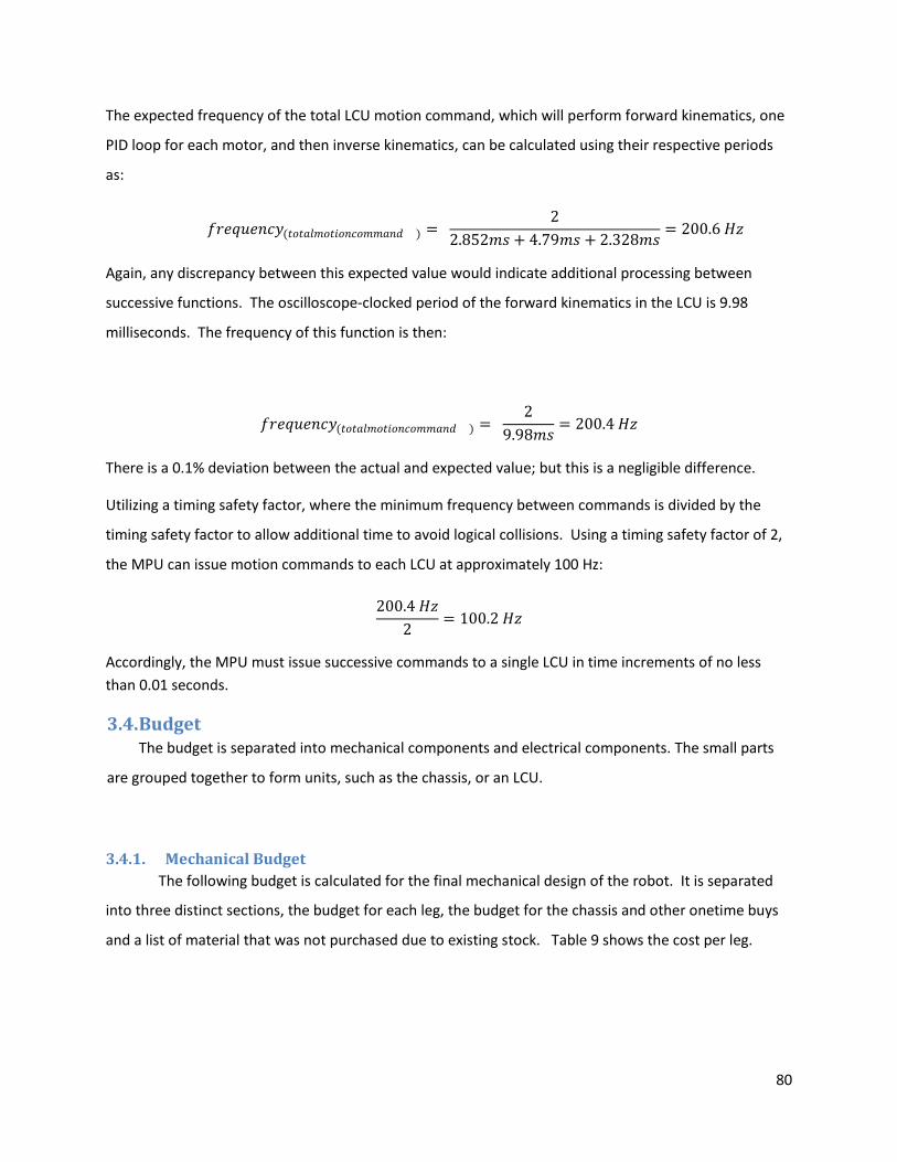
80
The expected frequency of the total LCU motion command, which will perform forward kinematics, one
PID loop for each motor, and then inverse kinematics, can be calculated using their respective periods
as:
𝑓𝑓𝑏𝑏𝑓𝑓𝑓𝑓𝑜𝑜𝑓𝑓𝑖𝑖𝑓𝑓𝑏𝑏(𝑜𝑜𝑜𝑜𝑜𝑜𝑏𝑏𝑠𝑠𝑚𝑚𝑜𝑜𝑜𝑜𝑖𝑖𝑜𝑜𝑖𝑖𝑓𝑓𝑜𝑜𝑚𝑚𝑚𝑚𝑏𝑏𝑖𝑖𝑑𝑑 ) = 2
2.852𝑚𝑚𝑜𝑜 + 4.79𝑚𝑚𝑜𝑜 + 2.328𝑚𝑚𝑜𝑜= 200.6 𝐻𝐻𝑜𝑜
Again, any discrepancy between this expected value would indicate additional processing between
successive functions. The oscilloscope-clocked period of the forward kinematics in the LCU is 9.98
milliseconds. The frequency of this function is then:
𝑓𝑓𝑏𝑏𝑓𝑓𝑓𝑓𝑜𝑜𝑓𝑓𝑖𝑖𝑓𝑓𝑏𝑏(𝑜𝑜𝑜𝑜𝑜𝑜𝑏𝑏𝑠𝑠𝑚𝑚𝑜𝑜𝑜𝑜𝑖𝑖𝑜𝑜𝑖𝑖𝑓𝑓𝑜𝑜𝑚𝑚𝑚𝑚𝑏𝑏𝑖𝑖𝑑𝑑 ) = 2
9.98𝑚𝑚𝑜𝑜= 200.4 𝐻𝐻𝑜𝑜
There is a 0.1% deviation between the actual and expected value; but this is a negligible difference.
Utilizing a timing safety factor, where the minimum frequency between commands is divided by the
timing safety factor to allow additional time to avoid logical collisions. Using a timing safety factor of 2,
the MPU can issue motion commands to each LCU at approximately 100 Hz:
200.4 𝐻𝐻𝑜𝑜2
= 100.2 𝐻𝐻𝑜𝑜
Accordingly, the MPU must issue successive commands to a single LCU in time increments of no less than 0.01 seconds.
3.4. Budget The budget is separated into mechanical components and electrical components. The small parts
are grouped together to form units, such as the chassis, or an LCU.
3.4.1. Mechanical Budget The following budget is calculated for the final mechanical design of the robot. It is separated
into three distinct sections, the budget for each leg, the budget for the chassis and other onetime buys
and a list of material that was not purchased due to existing stock. Table 9 shows the cost per leg.
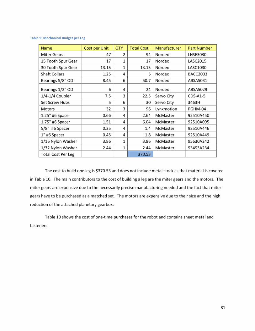
81
Table 9: Mechanical Budget per Leg
Name Cost per Unit QTY Total Cost Manufacturer Part Number Miter Gears 47 2 94 Nordex LHSE3030 15 Tooth Spur Gear 17 1 17 Nordex LASC2015 30 Tooth Spur Gear 13.15 1 13.15 Nordex LASC1030 Shaft Collars 1.25 4 5 Nordex BACC2003 Bearings 5/8" OD 8.45 6 50.7 Nordex ABSA5031
Bearings 1/2" OD 6 4 24 Nordex ABSA5029 1/4-1/4 Coupler 7.5 3 22.5 Servo City CDS-A1-5 Set Screw Hubs 5 6 30 Servo City 3463H Motors 32 3 96 Lynxmotion PGHM-04 1.25" #6 Spacer 0.66 4 2.64 McMaster 92510A450 1.75" #6 Spacer 1.51 4 6.04 McMaster 92510A095 5/8" #6 Spacer 0.35 4 1.4 McMaster 92510A446 1" #6 Spacer 0.45 4 1.8 McMaster 92510A449 1/16 Nylon Washer 3.86 1 3.86 McMaster 95630A242 1/32 Nylon Washer 2.44 1 2.44 McMaster 93493A234 Total Cost Per Leg 370.53
The cost to build one leg is $370.53 and does not include metal stock as that material is covered
in Table 10. The main contributors to the cost of building a leg are the miter gears and the motors. The
miter gears are expensive due to the necessarily precise manufacturing needed and the fact that miter
gears have to be purchased as a matched set. The motors are expensive due to their size and the high
reduction of the attached planetary gearbox.
Table 10 shows the cost of one-time purchases for the robot and contains sheet metal and
fasteners.
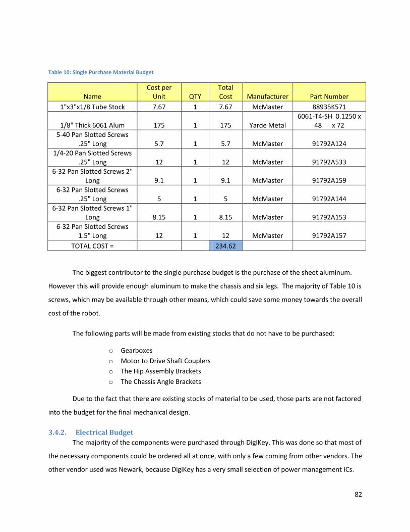
82
Table 10: Single Purchase Material Budget
Name Cost per
Unit QTY Total Cost Manufacturer Part Number
1"x3"x1/8 Tube Stock 7.67 1 7.67 McMaster 88935K571
1/8" Thick 6061 Alum 175 1 175 Yarde Metal 6061-T4-SH 0.1250 x
48 x 72 5-40 Pan Slotted Screws
.25" Long 5.7 1 5.7 McMaster 91792A124 1/4-20 Pan Slotted Screws
.25" Long 12 1 12 McMaster 91792A533 6-32 Pan Slotted Screws 2"
Long 9.1 1 9.1 McMaster 91792A159 6-32 Pan Slotted Screws
.25" Long 5 1 5 McMaster 91792A144 6-32 Pan Slotted Screws 1"
Long 8.15 1 8.15 McMaster 91792A153 6-32 Pan Slotted Screws
1.5" Long 12 1 12 McMaster 91792A157 TOTAL COST = 234.62
The biggest contributor to the single purchase budget is the purchase of the sheet aluminum.
However this will provide enough aluminum to make the chassis and six legs. The majority of Table 10 is
screws, which may be available through other means, which could save some money towards the overall
cost of the robot.
The following parts will be made from existing stocks that do not have to be purchased:
o Gearboxes o Motor to Drive Shaft Couplers o The Hip Assembly Brackets o The Chassis Angle Brackets
Due to the fact that there are existing stocks of material to be used, those parts are not factored
into the budget for the final mechanical design.
3.4.2. Electrical Budget The majority of the components were purchased through DigiKey. This was done so that most of
the necessary components could be ordered all at once, with only a few coming from other vendors. The
other vendor used was Newark, because DigiKey has a very small selection of power management ICs.
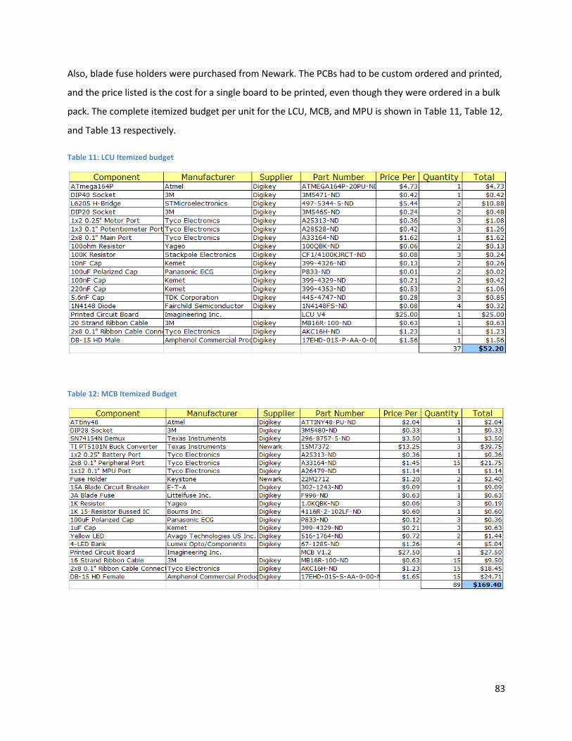
83
Also, blade fuse holders were purchased from Newark. The PCBs had to be custom ordered and printed,
and the price listed is the cost for a single board to be printed, even though they were ordered in a bulk
pack. The complete itemized budget per unit for the LCU, MCB, and MPU is shown in Table 11, Table 12,
and Table 13 respectively.
Table 11: LCU Itemized budget
Table 12: MCB Itemized Budget

84
Table 13: MPU Itemized Budget
4. Future Work Given the modular design of the robot, there are many potential areas for future work. The
most immediate task would be the construction of the final robot design including multiple leg modules.
Plans to complete this are already slated to be started following the submission of this project. The
balancing algorithm can be tested to show that the robot can identify its current configuration and
balance itself. From there, further work can be conducted to refine the algorithm and make it more
complex. For example, the algorithm can be developed to allow the robot to balance itself regardless of
the surface that the robot is standing on. The ultimate goal for the leg modules would be to allow the
robot to walk using any leg configuration.
Other possible areas of future work would be the development of new modules for the robot.
These modules can be generalized to include, but are not limited to, movement, manipulators and
sensors. Movement modules could come in the form of wheels to enable the robot travel at fast
speeds along roads, or treads for maneuvering through sand. Manipulators could come in the form of
an arm, a claw or gripper module. Sensors could be range finders, localization sensors or thermal
sensors. Other miscellaneous possible devices include a GPS sensor, which could be used to send the
robot to a predetermined location. Also, a RF receiver module could be created to add remote control
functionality to the robot. As long as the new modules follow the connection and communication
protocol, there is no limit to the modules that can be created. The only thing that must be done to
accommodate new modules is to program into the main processor how to handle this new module. The
robot can be developed for any task with the development of new modules.
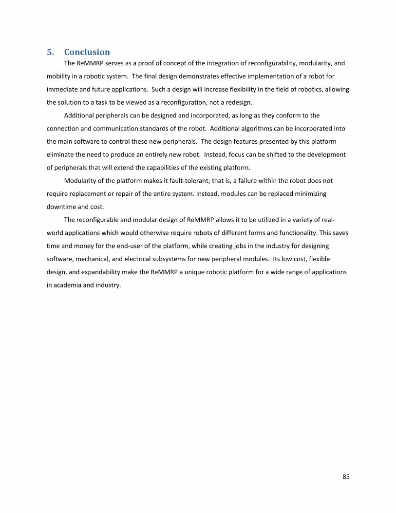
85
5. Conclusion The ReMMRP serves as a proof of concept of the integration of reconfigurability, modularity, and
mobility in a robotic system. The final design demonstrates effective implementation of a robot for
immediate and future applications. Such a design will increase flexibility in the field of robotics, allowing
the solution to a task to be viewed as a reconfiguration, not a redesign.
Additional peripherals can be designed and incorporated, as long as they conform to the
connection and communication standards of the robot. Additional algorithms can be incorporated into
the main software to control these new peripherals. The design features presented by this platform
eliminate the need to produce an entirely new robot. Instead, focus can be shifted to the development
of peripherals that will extend the capabilities of the existing platform.
Modularity of the platform makes it fault-tolerant; that is, a failure within the robot does not
require replacement or repair of the entire system. Instead, modules can be replaced minimizing
downtime and cost.
The reconfigurable and modular design of ReMMRP allows it to be utilized in a variety of real-
world applications which would otherwise require robots of different forms and functionality. This saves
time and money for the end-user of the platform, while creating jobs in the industry for designing
software, mechanical, and electrical subsystems for new peripheral modules. Its low cost, flexible
design, and expandability make the ReMMRP a unique robotic platform for a wide range of applications
in academia and industry.
86
6. References 1. Self-Reconfigurable Modular Robot -Experiments on Reconfiguration and Locomotion. Kamimura, Akiya, et al. 2001. International Conference on Intellegent Robots and Systems.
2. A Motion Planning Method for a Self-Reconfigurable Modular Robot. Kamimura, Akiya, et al. Maui, Hawaii : s.n., 2003. Internatioanl Conference on Intelligent Robots and Systems.
3. Towards Robotic Self-reassembly After Explosion. Dugan, Mike, et al. 2007. IEEE/RSJ International Conference on Intelligent Robots and Systems (IROS). pp. 2767-2772.
4. Blankespor, Kevin, et al. BigDog, the Rough-Terrain Quaduped Robot. 2008.
5. Atmel Corporation. ATmega 164P/324P/644P. [Datasheet] San Jose, CA : s.n., 2009.
6. Digi-Key Corporation. Digi-Key ATMEGA1281-16AU-ND (Manufacturer - ATMEGA1281-16AU). DigiKey Corp. | Electronic Components Distributor | United States Home Page. [Online] Digi-Key Corporation. [Cited: November 18, 2009.] http://search.digikey.com/scripts/DkSearch/dksus.dll?Detail&name=ATMEGA1281-16AU-ND.
7. —. Digi-Key - ATMEGA164PV-10PU-ND (Manufacturer - ATMEGA164PV-10PU). DigiKey Corp. | Electronic Components Distributor | United States Home Page. [Online] Digi-Key Corporation. [Cited: November 18, 2009.] http://search.digikey.com/scripts/DkSearch/dksus.dll?Detail&name=ATMEGA164PV-10PU-ND.
8. Atmel Corporation. ATmega640V/1280V/1281V/2560V/2561V. [Datasheet] San Jose, California : s.n., 2007.
9. Lynxmotion, Inc. Planetary Gear Motor - 12vdc 189:1 31rpm (4mm shaft). Lynxmotion Robotic Kits. [Online] Lynxmotion, Inc. [Cited: November 26, 2009.] http://www.lynxmotion.com/Product.aspx?productID=308&CategoryID=71.
10. —. Planetary Gear Motor - 12.0vdc 1:231 64rpm (4mm shaft). Lynxmotion Robot Kits. [Online] Lynxmotion, Inc. [Cited: December 12, 2009.] http://www.lynxmotion.com/Product.aspx?productID=580&CategoryID=71.
11. STMicroelectronics. L6205N DMOS Dual Full Bridge Driver. [Datasheet] Geneva, Switzerland : s.n., 2003.
12. Digi-Key Corporation. DigiKey Corp. | Electronic Components Distributor | United States Home Page. [Online] [Cited: March 11, 2010.] http://media.digikey.com/photos/Tyco%20Amp%20Photos/HEADER%202%20CIRC%20FIG%201A.jpg.
13. —. DigiKey Corp. | Electronic Components Distributor | United States Home Page. [Online] [Cited: March 11, 2010.] http://media.digikey.com/photos/Tyco%20Amp%20Photos/103639-2.jpg.
87
14. —. DigiKey Corp. | Electronic Components Distributor | United States Home Page. [Online] [Cited: March 11, 2010.] http://media.digikey.com/photos/Tyco%20Amp%20Photos/5103309-3.jpg.
15. —. DigiKey Corp. | Electronic Components Distributor | United States Home Page. [Online] [Cited: March 11, 2010.] http://media.digikey.com/photos/Tyco%20Amp%20Photos/534237-1.jpg.
16. —. DigiKey Corp. | Electronic Components Distributor | United States Home Page. [Online] [Cited: March 11, 2010.] http://media.digikey.com/photos/Tyco%20Amp%20Photos/534237-6.jpg.
17. —. DigiKey Corp. | Electronic Components Distributor | United States Home Page. [Online] [Cited: March 11, 2010.] http://media.digikey.com/photos/Sullins%20Photos/PPTC021LFBN-RC.jpg.
18. Bourns, Incorporated. 51/53 - Sealed 1/2” (12.5 mm) Square Control. [Datasheet] Riverside, California : s.n., 2009.
19. Texas Instruments. SN54154, SN74154 4-Line To16-Line Decoders/Demultiplexers. [Datasheet] Dallas, Texas : s.n., 1998.
20. Atmel Corporation. ATtiny48/88. [Datasheet] San Jose, CA : s.n., 2009.
21. Aivaka. Linear or LDO Regulators & Step-Down Switching Regulators. [Datasheet] San Jose, CA : s.n., 2007.
22. XP Power. DC-DC 1 Watt IV Series. [Datasheet] Sunnyvale, California : s.n., 2009.
23. Texas Instruments. PT 5100 Series 1-A Positive Step-Down Integrated Switching Regulator. [Datasheet] Dallas, Texas : s.n., 2001.
24. Kugelstadt, Thomas. Understanding the SPI bus' structure, operation. EETimes-India. [Online] July 28, 2009. [Cited: October 19, 2009.] http://www.eetindia.co.in/STATIC/PDF/200907/EEIOL_2009JUL29_INTD_EMS_TA_01.pdf?SOURCES=DOWNLOAD.
25. Reed, Kenneth D. Introduction to Networking. Arvada, CO : WestNet Learning Technologies, 2001.
26. Spong, Mark W., Hutchinson, Seth and Vidyasagar, M. Robot Modeling and Control. Hoboken, NJ : John Wiley & Sons, Inc., 2006.
27. Craig, John J. Intorduction to Robotics. Upper Saddle River : Pearson Education, Inc., 2005.
28. Lathi, B. P. Linear Systems and Signals. New York, NY : Oxford University Press, Inc., 2005.
29. Kaiser, David. Fundamentals of Servo Motion Control. Rohnert Park, CA : s.n., July 11, 2001.
30. Optimum Settings for Automatic Controllers. Ziegler, J. G. and Nichols, N. B. 1942, Transactions of the American Society of Mechanical Engineers, pp. 759-768.
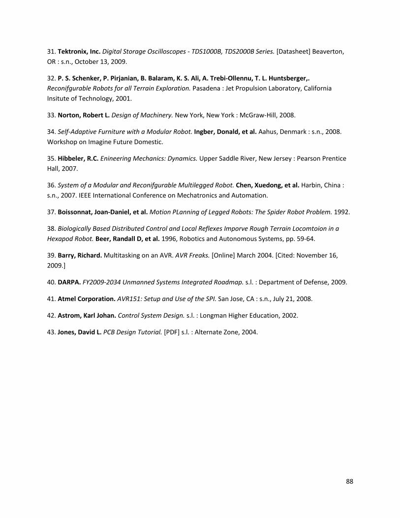
88
31. Tektronix, Inc. Digital Storage Oscilloscopes - TDS1000B, TDS2000B Series. [Datasheet] Beaverton, OR : s.n., October 13, 2009.
32. P. S. Schenker, P. Pirjanian, B. Balaram, K. S. Ali, A. Trebi-Ollennu, T. L. Huntsberger,. Reconifgurable Robots for all Terrain Exploration. Pasadena : Jet Propulsion Laboratory, California Insitute of Technology, 2001.
33. Norton, Robert L. Design of Machinery. New York, New York : McGraw-Hill, 2008.
34. Self-Adaptive Furniture with a Modular Robot. Ingber, Donald, et al. Aahus, Denmark : s.n., 2008. Workshop on Imagine Future Domestic.
35. Hibbeler, R.C. Enineering Mechanics: Dynamics. Upper Saddle River, New Jersey : Pearson Prentice Hall, 2007.
36. System of a Modular and Reconifgurable Multilegged Robot. Chen, Xuedong, et al. Harbin, China : s.n., 2007. IEEE International Conference on Mechatronics and Automation.
37. Boissonnat, Joan-Daniel, et al. Motion PLanning of Legged Robots: The Spider Robot Problem. 1992.
38. Biologically Based Distributed Control and Local Reflexes Imporve Rough Terrain Locomtoion in a Hexapod Robot. Beer, Randall D, et al. 1996, Robotics and Autonomous Systems, pp. 59-64.
39. Barry, Richard. Multitasking on an AVR. AVR Freaks. [Online] March 2004. [Cited: November 16, 2009.]
40. DARPA. FY2009-2034 Unmanned Systems Integrated Roadmap. s.l. : Department of Defense, 2009.
41. Atmel Corporation. AVR151: Setup and Use of the SPI. San Jose, CA : s.n., July 21, 2008.
42. Astrom, Karl Johan. Control System Design. s.l. : Longman Higher Education, 2002.
43. Jones, David L. PCB Design Tutorial. [PDF] s.l. : Alternate Zone, 2004.

89
7. Appendices
7.1. LCU Schematics
(Beginning on the following page)
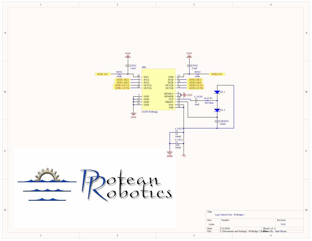
1
1
2
2
3
3
4
4
D D
C C
B B
A A
Title
Number RevisionSize
Letter
Date: 2/15/2010 Sheet ofFile: C:\Documents and Settings\..\H-Bridge 1.SchDocDrawn By:
IN1A1
IN2A2
SENSEA 3
OUT1A4
GND5
GND6
OUT1B 7
SENSEB 8
IN1B 9
IN2B 10
ENB 11
VBOOT 12
OUT2B 13
VSB 14
GND15
GND16 VSA 17
OUT2A18
VCP 19
ENA20
HB1
L6205 H-Bridge
GND
MTR2-EN
MTR1-SIG1 MTR2-SIG1MTR2-SIG2MTR1-SIG2
MTR1-EN
MTR1-OUTAMTR1-OUTB
MTR2-OUTAMTR2-OUTB
100K
REN2
100K
REN15.6nFCEN2
5.6nFCEN1
GNDGND
10nF
C-VCP1
100 Ohm
R-VCP1
D1-1
D1-2
220nFCBOOT1
GND
100nF
C-VS12
100uF
C-VS11
+12GND
Leg Control Unit - H-Bridge 1
V4.0
2 4Matt Bienia
PIC0VCP101 PIC0VCP102
COC0VCP1
PIC0VS1101PIC0VS1102
COC0VS11
PIC0VS1201 PIC0VS1202
COC0VS12
PICBOOT101
PICBOOT102COCBOOT1
PICEN101
PICEN102COCEN1
PICEN201
PICEN202COCEN2
PID10101PID10102
COD101
PID10201PID10202
COD102
PIHB101
PIHB102
PIHB103
PIHB104
PIHB105
PIHB106
PIHB107
PIHB108
PIHB109
PIHB1010
PIHB1011
PIHB1012
PIHB1013
PIHB1014
PIHB1015
PIHB1016 PIHB1017
PIHB1018
PIHB1019
PIHB1020
COHB1
PIR0VCP101 PIR0VCP102COR0VCP1
PIREN101 PIREN102COREN1
PIREN201 PIREN202COREN2
POMTR10EN
POMTR10OUTAPOMTR10OUTB
POMTR10SIG1POMTR10SIG2
POMTR20EN
POMTR20OUTAPOMTR20OUTB
POMTR20SIG1POMTR20SIG2
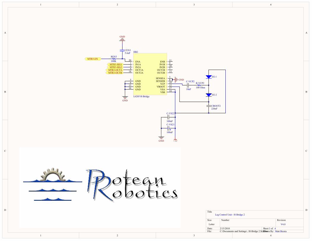
1
1
2
2
3
3
4
4
D D
C C
B B
A A
Title
Number RevisionSize
Letter
Date: 2/15/2010 Sheet ofFile: C:\Documents and Settings\..\H-Bridge 2.SchDocDrawn By:
GND
MTR3-EN
MTR3-SIG1MTR3-SIG2
MTR3-OUTAMTR3-OUTB
100K
REN35.6nFCEN3
GND
IN1A1
IN2A2
SENSEA 3
OUT1A4
GND5
GND6
OUT1B 7
SENSEB 8
IN1B 9
IN2B 10
ENB 11
VBOOT 12
OUT2B 13
VSB 14
GND15
GND16 VSA 17
OUT2A18
VCP 19
ENA20
HB2
L6205 H-Bridge
10nF
C-VCP2
100 Ohm
R-VCP2
D2-1
D2-2
220nFCBOOT2
GND
100nF
C-VS22
100uF
C-VS21
+12GND
Leg Control Unit - H-Bridge 2
V4.0
3 4Matt Bienia
PIC0VCP201 PIC0VCP202
COC0VCP2
PIC0VS2101PIC0VS2102
COC0VS21
PIC0VS2201 PIC0VS2202
COC0VS22
PICBOOT201
PICBOOT202COCBOOT2
PICEN301
PICEN302COCEN3
PID20101PID20102
COD201
PID20201PID20202
COD202
PIHB201
PIHB202
PIHB203
PIHB204
PIHB205
PIHB206
PIHB207
PIHB208
PIHB209
PIHB2010
PIHB2011
PIHB2012
PIHB2013
PIHB2014
PIHB2015
PIHB2016 PIHB2017
PIHB2018
PIHB2019
PIHB2020
COHB2
PIR0VCP201 PIR0VCP202COR0VCP2
PIREN301 PIREN302COREN3
POMTR30EN
POMTR30OUTAPOMTR30OUTB
POMTR30SIG1POMTR30SIG2
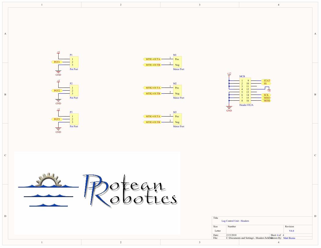
1
1
2
2
3
3
4
4
D D
C C
B B
A A
Title
Number RevisionSize
Letter
Date: 2/15/2010 Sheet ofFile: C:\Documents and Settings\..\Headers.SchDocDrawn By:
123
P1
Pot Port
123
P2
Pot Port
123
P3
Pot Port
GND
GND
+5
+5
+5
POT1
POT2
POT3
GNDMOSIMISOSCK
SSSTAT
+5
MTR3-OUTA
MTR3-OUTB
MTR2-OUTA
MTR2-OUTB
MTR1-OUTA
MTR1-OUTB
Pos1
Neg2
M1
Motor Port
Pos1
Neg2
M2
Motor Port
Pos1
Neg2
M3
Motor Port
Leg Control Unit - Headers
V4.0
4 4Matt Bienia
12345678
910111213141516
MCB
Header 8X2A
GND
+12
PIM101
PIM102
COM1
PIM201
PIM202
COM2
PIM301
PIM302
COM3
PIMCB01
PIMCB02
PIMCB03
PIMCB04
PIMCB05
PIMCB06
PIMCB07
PIMCB08
PIMCB09
PIMCB010
PIMCB011
PIMCB012
PIMCB013
PIMCB014
PIMCB015
PIMCB016
COMCB
PIP101
PIP102
PIP103
COP1
PIP201
PIP202
PIP203
COP2
PIP301
PIP302
PIP303
COP3
POMISOPOMOSI
POMTR10OUTA
POMTR10OUTB
POMTR20OUTA
POMTR20OUTB
POMTR30OUTA
POMTR30OUTB
POPOT1
POPOT2
POPOT3
POSCK
POSSPOSTAT
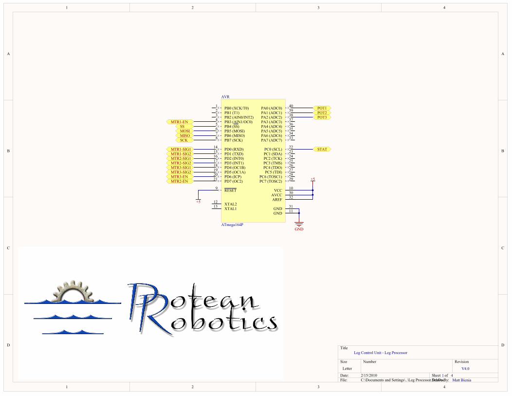
1
1
2
2
3
3
4
4
D D
C C
B B
A A
Title
Number RevisionSize
Letter
Date: 2/15/2010 Sheet ofFile: C:\Documents and Settings\..\Leg Processor.SchDocDrawn By:
PB0 (XCK/T0)1
PB1 (T1)2
PB2 (AIN0/INT2)3
PB3 (AIN1/OC0)4
PB4 (SS)5
PB5 (MOSI)6
PB6 (MISO)7
PB7 (SCK)8
RESET9
PD0 (RXD)14
PD1 (TXD)15
PD2 (INT0)16
PD3 (INT1)17
PD4 (OC1B)18
PD5 (OC1A)19
PD6 (ICP)20
PD7 (OC2)21
XTAL212
XTAL113
GND 11
PC0 (SCL) 22
PC1 (SDA) 23
PC2 (TCK) 24
PC3 (TMS) 25
PC4 (TDO) 26
PC5 (TDI) 27
PC6 (TOSC1) 28
PC7 (TOSC2) 29
AREF 32AVCC 30
GND 31
PA7 (ADC7) 33PA6 (ADC6) 34PA5 (ADC5) 35PA4 (ADC4) 36PA3 (ADC3) 37PA2 (ADC2) 38PA1 (ADC1) 39PA0 (ADC0) 40
VCC 10
AVR
ATmega164PGND
+5
SSMOSIMISOSCK
POT1POT2POT3
MTR1-EN
MTR2-ENMTR3-EN
MTR1-SIG1
MTR2-SIG1MTR2-SIG2MTR3-SIG1MTR3-SIG2
MTR1-SIG2STAT
Leg Control Unit - Leg Processor
V4.0
1 4Matt Bienia
+5
PIAVR01
PIAVR02
PIAVR03
PIAVR04
PIAVR05
PIAVR06
PIAVR07
PIAVR08
PIAVR09 PIAVR010
PIAVR011
PIAVR012
PIAVR013
PIAVR014
PIAVR015
PIAVR016
PIAVR017
PIAVR018
PIAVR019
PIAVR020
PIAVR021
PIAVR022
PIAVR023
PIAVR024
PIAVR025
PIAVR026
PIAVR027
PIAVR028
PIAVR029
PIAVR030
PIAVR031
PIAVR032
PIAVR033
PIAVR034
PIAVR035
PIAVR036
PIAVR037
PIAVR038
PIAVR039
PIAVR040
COAVR
POMISOPOMOSI
POMTR10EN
POMTR10SIG1POMTR10SIG2
POMTR20EN
POMTR20SIG1POMTR20SIG2
POMTR30EN
POMTR30SIG1POMTR30SIG2
POPOT1POPOT2POPOT3
POSCK
POSS
POSTAT
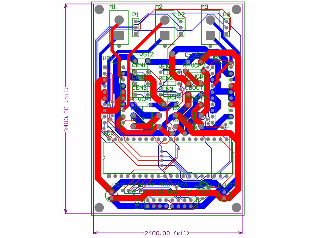
CO
PAAVR01 PAAVR02 PAAVR03 PAAVR04 PAAVR05 PAAVR06 PAAVR07 PAAVR08 PAAVR09 PAAVR010 PAAVR011 PAAVR012 PAAVR013 PAAVR014 PAAVR015 PAAVR016 PAAVR017 PAAVR018 PAAVR019 PAAVR020
PAAVR040 PAAVR039 PAAVR038 PAAVR037 PAAVR036 PAAVR035 PAAVR034 PAAVR033 PAAVR032 PAAVR031 PAAVR030 PAAVR029 PAAVR028 PAAVR027 PAAVR026 PAAVR025 PAAVR024 PAAVR023 PAAVR022 PAAVR021
COAVR
PAC0VCP102PAC0VCP101
COC0VCP1
PAC0VCP202PAC0VCP201
COC0VCP2
PAC0VS1101
PAC0VS1102
COC0VS11
PAC0VS1202 PAC0VS1201
COC0VS12
PAC0VS2101
PAC0VS2102
COC0VS21
PAC0VS2202PAC0VS2201
COC0VS22
PACBOOT102PACBOOT101
COCBOOT1
PACBOOT202PACBOOT201
COCBOOT2
PACEN102PACEN101
COCEN1
PACEN202PACEN201
COCEN2
PACEN302PACEN301
COCEN3
PAD10102PAD10101
COD101
PAD10202PAD10201
COD102PAD20101 PAD20102
COD201
PAD20201 PAD20202
COD202
PAHB101
PAHB102
PAHB103
PAHB104
PAHB105
PAHB106
PAHB107
PAHB108
PAHB109
PAHB1010
PAHB1020
PAHB1019
PAHB1018
PAHB1017
PAHB1016
PAHB1015
PAHB1014
PAHB1013
PAHB1012
PAHB1011
COHB1
PAHB201
PAHB202
PAHB203
PAHB204
PAHB205
PAHB206
PAHB207
PAHB208
PAHB209
PAHB2010
PAHB2020
PAHB2019
PAHB2018
PAHB2017
PAHB2016
PAHB2015
PAHB2014
PAHB2013
PAHB2012
PAHB2011
COHB2
PAM101
PAM102
PAM103
COM1
PAM201
PAM202
PAM203
COM2
PAM301
PAM302
PAM303
COM3
PAMCB01 PAMCB02 PAMCB03 PAMCB04 PAMCB05 PAMCB06 PAMCB07 PAMCB08
PAMCB09 PAMCB010 PAMCB011 PAMCB012 PAMCB013 PAMCB014 PAMCB015 PAMCB016COMCB
PAP101
PAP102
PAP103
COP1
PAP201
PAP202
PAP203
COP2
PAP301
PAP302
PAP303
COP3
PAR0VCP102 PAR0VCP101
COR0VCP1
PAR0VCP202PAR0VCP201
COR0VCP2
PAREN102PAREN101
COREN1
PAREN202PAREN201
COREN2
PAREN302PAREN301
COREN3
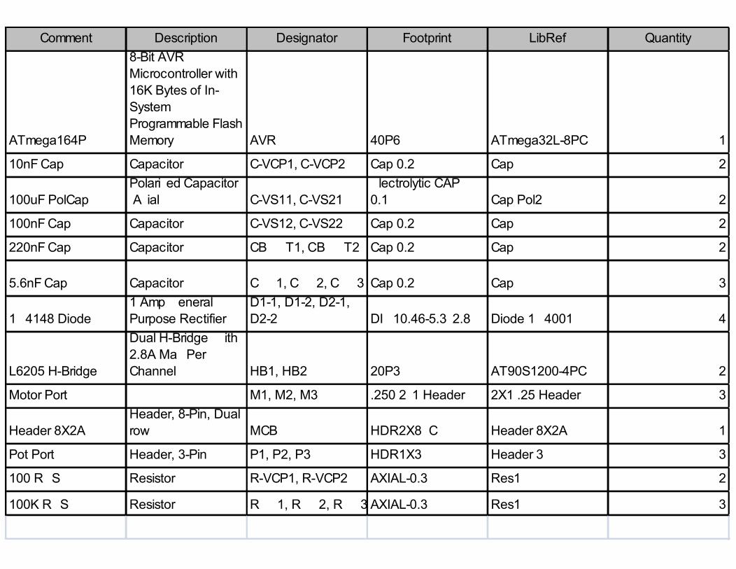
Comment Description Designator Footprint LibRef Quantity
ATmega164P
8-Bit AVR Microcontroller with 16K Bytes of In-System Programmable Flash Memory AVR 40P6 ATmega32L-8PC 1
10nF Cap Capacitor C-VCP1, C-VCP2 Cap 0.2" Cap 2
100uF PolCapPolarized Capacitor (Axial) C-VS11, C-VS21
Electrolytic CAP 0.1" Cap Pol2 2
100nF Cap Capacitor C-VS12, C-VS22 Cap 0.2" Cap 2
220nF Cap Capacitor CBOOT1, CBOOT2 Cap 0.2" Cap 2
5.6nF Cap Capacitor CEN1, CEN2, CEN3 Cap 0.2" Cap 3
1N4148 Diode1 Amp General Purpose Rectifier
D1-1, D1-2, D2-1, D2-2 DIO10.46-5.3x2.8 Diode 1N4001 4
L6205 H-Bridge
Dual H-Bridge With 2.8A Max Per Channel HB1, HB2 20P3 AT90S1200-4PC 2
Motor Port M1, M2, M3 .250 2x1 Header 2X1 .25 Header 3
Header 8X2AHeader, 8-Pin, Dual row MCB HDR2X8_CEN Header 8X2A 1
Pot Port Header, 3-Pin P1, P2, P3 HDR1X3 Header 3 3
100 RES Resistor R-VCP1, R-VCP2 AXIAL-0.3 Res1 2
100K RES Resistor REN1, REN2, REN3 AXIAL-0.3 Res1 3

96
7.2. MCB Schematics
(Beginning on the following page)
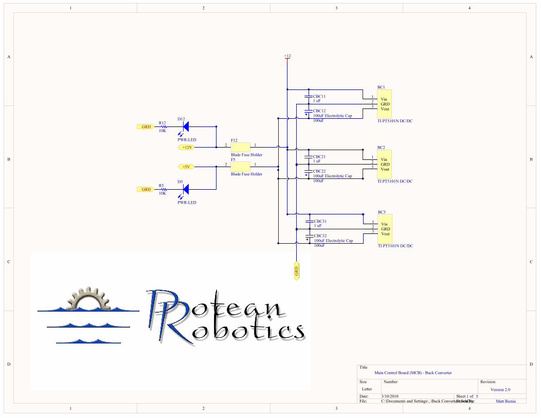
1
1
2
2
3
3
4
4
D D
C C
B B
A A
Title
Number RevisionSize
Letter
Date: 3/10/2010 Sheet ofFile: C:\Documents and Settings\..\Buck Converters.SchDocDrawn By:
+12
+12V
+5V
Main Control Board (MCB) - Buck Converter
Version 2.01 5
Matt Bienia
10K
R12
10K
R5
GRD
GRD
Vin1
GRD2
Vout3
BC1
TI PT5101N DC/DC
Vin1
GRD2
Vout3
BC2
TI PT5101N DC/DC
Vin1
GRD2
Vout3
BC3
TI PT5101N DC/DC
D12
PWR-LED
D5
PWR-LED
12F12
Blade Fuse Holder
12F5
Blade Fuse Holder
GR
D
1 uFCBC21
100uF
CBC22100uF Electrolytic Cap
1 uFCBC11
100uF
CBC12100uF Electrolytic Cap
1 uFCBC31
100uF
CBC32100uF Electrolytic Cap
PIBC101
PIBC102
PIBC103
COBC1
PIBC201
PIBC202
PIBC203
COBC2
PIBC301
PIBC302
PIBC303
COBC3
PICBC1101
PICBC1102COCBC11
PICBC1201
PICBC1202COCBC12
PICBC2101
PICBC2102COCBC21
PICBC2201
PICBC2202COCBC22
PICBC3101
PICBC3102COCBC31
PICBC3201
PICBC3202COCBC32
PID501PID502
COD5
PID1201PID1202
COD12
PIF501PIF502
COF5
PIF1201PIF1202
COF12
PIR501 PIR502COR5
PIR1201 PIR1202COR12
PIBC101
PIBC201
PIBC301
PICBC1102
PICBC2102
PICBC3102
PIF1201
PID1202PIR1202 PID1201
PIF1202PO012V
PID502PIR502 PID501
PIF502PO05V
PIBC103
PIBC203
PIBC303
PICBC1201
PICBC2201
PICBC3201
PIF501
PIBC102
PIBC202
PIBC302
PICBC1101PICBC1202
PICBC2101PICBC2202
PICBC3101PICBC3202
PIR501
PIR1201POGRD
PO05V
PO012V
POGRD
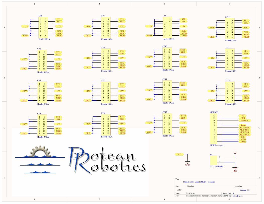
1
1
2
2
3
3
4
4
D D
C C
B B
A A
Title
Number RevisionSize
Letter
Date: 3/10/2010 Sheet ofFile: C:\Documents and Settings\..\Headers.SchDocDrawn By:
Main Control Board (MCB) - Headers
Version 1.25 5
Matt Bienia
SS1
SS2
SS3
ST1
ST2
ST3
SS4
SS5
SS6
SS7
SS8
SS9
ST4
ST5
ST6
ST7
ST8
ST9
SS10
SS11
SS12
ST10
ST11
ST12
SS13ST13
SS14ST14
SS15ST15
Status
MOSIMISOSCK
+5V
MOSIMISOSCK
+5V
MOSIMISOSCK
+5V
MOSIMISOSCK
+5V
MOSIMISOSCK
+5V
MOSIMISOSCK
+5V
MOSIMISOSCK
+5V
MOSIMISOSCK
+5V
MOSIMISOSCK
+5V
MOSIMISOSCK
+5V
MOSIMISOSCK
+5V
MOSIMISOSCK
+5V
MOSIMISOSCK
+5V
MOSIMISOSCK
+5V
MOSIMISOSCK
GRD
+5V+12V
MCU-SSAMCU-SSBMCU-SSCMCU-SSD
MOSIMISOSCK
GND
+12
+5V
GRD
GND
123456789
101112
MCU-CP
MCU Connector
GRDMUXEN
1
2
BC
2X1 .25 Header
12345678
910111213141516
CP1
Header 8X2A
12345678
910111213141516
CP3
Header 8X2A
12345678
910111213141516
CP4
Header 8X2A
12345678
910111213141516
CP5
Header 8X2A
12345678
910111213141516
CP6
Header 8X2A
12345678
910111213141516
CP7
Header 8X2A
12345678
910111213141516
CP8
Header 8X2A
12345678
910111213141516
CP9
Header 8X2A
12345678
910111213141516
CP10
Header 8X2A
12345678
910111213141516
CP11
Header 8X2A
12345678
910111213141516
CP12
Header 8X2A
12345678
910111213141516
CP13
Header 8X2A
12345678
910111213141516
CP14
Header 8X2A
12345678
910111213141516
CP15
Header 8X2A
12345678
910111213141516
CP2
Header 8X2A
GRD
+12V
GRD
+12V
GRD
+12V
GRD
+12V
GRD
+12V
GRD
+12V
GRD
+12V
GRD
+12V
GRD
+12V
GRD
+12V
GRD
+12V
GRD
+12V
GRD
+12V
GRD
+12V
PIBC01
PIBC02
COBC
PICP101
PICP102
PICP103
PICP104
PICP105
PICP106
PICP107
PICP108
PICP109
PICP1010
PICP1011
PICP1012
PICP1013
PICP1014
PICP1015
PICP1016
COCP1
PICP201
PICP202
PICP203
PICP204
PICP205
PICP206
PICP207
PICP208
PICP209
PICP2010
PICP2011
PICP2012
PICP2013
PICP2014
PICP2015
PICP2016
COCP2
PICP301
PICP302
PICP303
PICP304
PICP305
PICP306
PICP307
PICP308
PICP309
PICP3010
PICP3011
PICP3012
PICP3013
PICP3014
PICP3015
PICP3016
COCP3
PICP401
PICP402
PICP403
PICP404
PICP405
PICP406
PICP407
PICP408
PICP409
PICP4010
PICP4011
PICP4012
PICP4013
PICP4014
PICP4015
PICP4016
COCP4
PICP501
PICP502
PICP503
PICP504
PICP505
PICP506
PICP507
PICP508
PICP509
PICP5010
PICP5011
PICP5012
PICP5013
PICP5014
PICP5015
PICP5016
COCP5
PICP601
PICP602
PICP603
PICP604
PICP605
PICP606
PICP607
PICP608
PICP609
PICP6010
PICP6011
PICP6012
PICP6013
PICP6014
PICP6015
PICP6016
COCP6
PICP701
PICP702
PICP703
PICP704
PICP705
PICP706
PICP707
PICP708
PICP709
PICP7010
PICP7011
PICP7012
PICP7013
PICP7014
PICP7015
PICP7016
COCP7
PICP801
PICP802
PICP803
PICP804
PICP805
PICP806
PICP807
PICP808
PICP809
PICP8010
PICP8011
PICP8012
PICP8013
PICP8014
PICP8015
PICP8016
COCP8
PICP901
PICP902
PICP903
PICP904
PICP905
PICP906
PICP907
PICP908
PICP909
PICP9010
PICP9011
PICP9012
PICP9013
PICP9014
PICP9015
PICP9016
COCP9
PICP1001
PICP1002
PICP1003
PICP1004
PICP1005
PICP1006
PICP1007
PICP1008
PICP1009
PICP10010
PICP10011
PICP10012
PICP10013
PICP10014
PICP10015
PICP10016
COCP10
PICP1101
PICP1102
PICP1103
PICP1104
PICP1105
PICP1106
PICP1107
PICP1108
PICP1109
PICP11010
PICP11011
PICP11012
PICP11013
PICP11014
PICP11015
PICP11016
COCP11
PICP1201
PICP1202
PICP1203
PICP1204
PICP1205
PICP1206
PICP1207
PICP1208
PICP1209
PICP12010
PICP12011
PICP12012
PICP12013
PICP12014
PICP12015
PICP12016
COCP12
PICP1301
PICP1302
PICP1303
PICP1304
PICP1305
PICP1306
PICP1307
PICP1308
PICP1309
PICP13010
PICP13011
PICP13012
PICP13013
PICP13014
PICP13015
PICP13016
COCP13
PICP1401
PICP1402
PICP1403
PICP1404
PICP1405
PICP1406
PICP1407
PICP1408
PICP1409
PICP14010
PICP14011
PICP14012
PICP14013
PICP14014
PICP14015
PICP14016
COCP14
PICP1501
PICP1502
PICP1503
PICP1504
PICP1505
PICP1506
PICP1507
PICP1508
PICP1509
PICP15010
PICP15011
PICP15012
PICP15013
PICP15014
PICP15015
PICP15016
COCP15
PIMCU0CP01
PIMCU0CP02
PIMCU0CP03
PIMCU0CP04
PIMCU0CP05
PIMCU0CP06
PIMCU0CP07
PIMCU0CP08
PIMCU0CP09
PIMCU0CP010
PIMCU0CP011
PIMCU0CP012
COMCU0CP
PIBC01
PIBC02
PICP105
PICP106
PICP107
PICP108
PICP205
PICP206
PICP207
PICP208
PICP305
PICP306
PICP307
PICP308
PICP405
PICP406
PICP407
PICP408
PICP505
PICP506
PICP507
PICP508
PICP605
PICP606
PICP607
PICP608
PICP705
PICP706
PICP707
PICP708
PICP805
PICP806
PICP807
PICP808
PICP905
PICP906
PICP907
PICP908
PICP1005
PICP1006
PICP1007
PICP1008
PICP1105
PICP1106
PICP1107
PICP1108
PICP1205
PICP1206
PICP1207
PICP1208
PICP1305
PICP1306
PICP1307
PICP1308
PICP1405
PICP1406
PICP1407
PICP1408
PICP1505
PICP1506
PICP1507
PICP1508
PIMCU0CP011
POGRD
PIMCU0CP010 POMUXENPIMCU0CP09
PIMCU0CP08 POStatusPIMCU0CP07 POMCU0SSDPIMCU0CP06 POMCU0SSCPIMCU0CP05 POMCU0SSBPIMCU0CP04 POMCU0SSA
PICP1016
PICP2016
PICP3016
PICP4016
PICP5016
PICP6016
PICP7016
PICP8016
PICP9016
PICP10016
PICP11016
PICP12016
PICP13016
PICP14016
PICP15016
PIMCU0CP01
POMOSI
PICP1015
PICP2015
PICP3015
PICP4015
PICP5015
PICP6015
PICP7015
PICP8015
PICP9015
PICP10015
PICP11015
PICP12015
PICP13015
PICP14015
PICP15015
PIMCU0CP02
POMISO
PICP1014
PICP2014
PICP3014
PICP4014
PICP5014
PICP6014
PICP7014
PICP8014
PICP9014
PICP10014
PICP11014
PICP12014
PICP13014
PICP14014
PICP15014
PIMCU0CP03
POSCKPICP15013
PICP1012
PICP2012
PICP3012
PICP4012
PICP5012
PICP6012
PICP7012
PICP8012
PICP9012
PICP10012
PICP11012
PICP12012
PICP13012
PICP14012
PICP15012
PIMCU0CP012
PO05VPICP15011
PICP15010 POSS15PICP1509 POST15
PICP101
PICP102
PICP103
PICP104
PICP201
PICP202
PICP203
PICP204
PICP301
PICP302
PICP303
PICP304
PICP401
PICP402
PICP403
PICP404
PICP501
PICP502
PICP503
PICP504
PICP601
PICP602
PICP603
PICP604
PICP701
PICP702
PICP703
PICP704
PICP801
PICP802
PICP803
PICP804
PICP901
PICP902
PICP903
PICP904
PICP1001
PICP1002
PICP1003
PICP1004
PICP1101
PICP1102
PICP1103
PICP1104
PICP1201
PICP1202
PICP1203
PICP1204
PICP1301
PICP1302
PICP1303
PICP1304
PICP1401
PICP1402
PICP1403
PICP1404
PICP1501
PICP1502
PICP1503
PICP1504PO012V
PICP14013
PICP14011
PICP14010 POSS14PICP1409 POST14
PICP13013
PICP13011
PICP13010 POSS13PICP1309 POST13
PICP12013
PICP12011
PICP12010 POSS12PICP1209 POST12
PICP11013
PICP11011
PICP11010 POSS11PICP1109 POST11
PICP10013
PICP10011
PICP10010 POSS10PICP1009 POST10
PICP9013
PICP9011
PICP9010 POSS9PICP909 POST9
PICP8013
PICP8011
PICP8010 POSS8PICP809 POST8
PICP7013
PICP7011
PICP7010 POSS7PICP709 POST7
PICP6013
PICP6011
PICP6010 POSS6PICP609 POST6
PICP5013
PICP5011
PICP5010 POSS5PICP509 POST5
PICP4013
PICP4011
PICP4010 POSS4PICP409 POST4
PICP3013
PICP3011
PICP3010 POSS3PICP309 POST3
PICP2013
PICP2011
PICP2010 POSS2PICP209 POST2
PICP1013
PICP1011
PICP1010 POSS1PICP109 POST1
PO05VPO012V
POGRD
POMCU0SSAPOMCU0SSBPOMCU0SSCPOMCU0SSD
POMISOPOMOSI
POMUXEN
POSCK
POSS1
POSS2
POSS3
POSS4
POSS5
POSS6
POSS7
POSS8
POSS9
POSS10
POSS11
POSS12
POSS13
POSS14
POSS15
POST1
POST2
POST3
POST4
POST5
POST6
POST7
POST8
POST9
POST10
POST11
POST12
POST13
POST14
POST15
POSTATUS
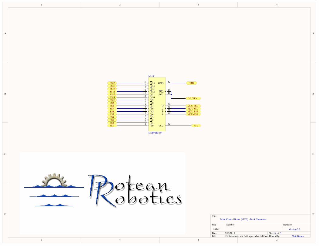
1
1
2
2
3
3
4
4
D D
C C
B B
A A
Title
Number RevisionSize
Letter
Date: 3/10/2010 Sheet ofFile: C:\Documents and Settings\..\Mux.SchDoc Drawn By:
Y01 Y12 Y23 Y34 Y45 Y56 Y67 Y78 Y89 Y910 Y1011
GND 12
Y1113 Y1214 Y1315 Y1416 Y1517
OE1 18OE2 19
D 20
C 21
B 22
A 23
VCC 24
MUX
MM74HC154
SS16SS15SS14SS13SS12SS11SS10
SS2
SS9SS8SS7SS6SS5SS4SS3
SS1 +5V
MCU-SSAMCU-SSBMCU-SSCMCU-SSD
Main Control Board (MCB) - Buck Converter
Version 2.03 5
Matt Bienia
MUXEN
GRD
PIMUX01
PIMUX02
PIMUX03
PIMUX04
PIMUX05
PIMUX06
PIMUX07
PIMUX08
PIMUX09
PIMUX010
PIMUX011
PIMUX012
PIMUX013
PIMUX014
PIMUX015
PIMUX016
PIMUX017
PIMUX018
PIMUX019
PIMUX020
PIMUX021
PIMUX022
PIMUX023
PIMUX024
COMUX
PIMUX024 PO05V
PIMUX023 POMCU0SSAPIMUX022 POMCU0SSBPIMUX021 POMCU0SSCPIMUX020 POMCU0SSD
PIMUX018
PIMUX019
POMUXEN
PIMUX017POSS16PIMUX016POSS15PIMUX015POSS14PIMUX014POSS13PIMUX013POSS12
PIMUX012 POGRD
PIMUX011POSS11PIMUX010POSS10PIMUX09POSS9PIMUX08POSS8PIMUX07POSS7PIMUX06POSS6PIMUX05POSS5PIMUX04POSS4PIMUX03POSS3PIMUX02POSS2PIMUX01POSS1 PO05V
POGRD
POMCU0SSAPOMCU0SSBPOMCU0SSCPOMCU0SSD
POMUXEN
POSS1POSS2POSS3POSS4POSS5POSS6POSS7POSS8POSS9POSS10POSS11POSS12POSS13POSS14POSS15POSS16
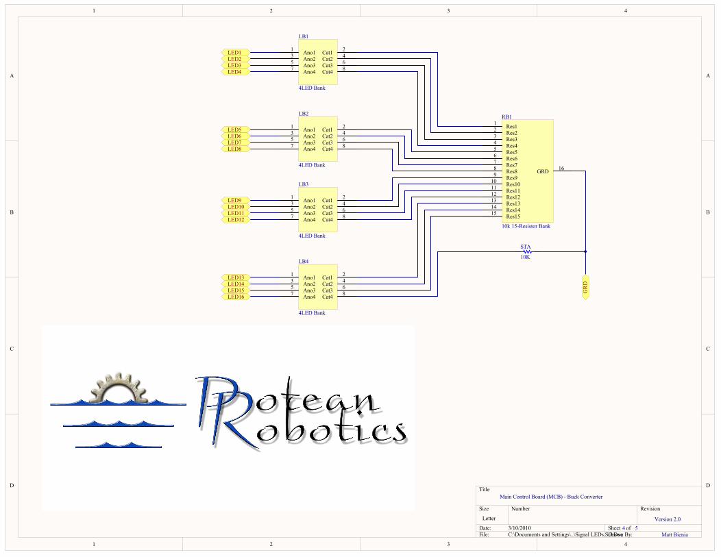
1
1
2
2
3
3
4
4
D D
C C
B B
A A
Title
Number RevisionSize
Letter
Date: 3/10/2010 Sheet ofFile: C:\Documents and Settings\..\Signal LEDs.SchDocDrawn By:
Res11
Res22
Res33
Res44
Res55
Res66
Res77
Res88
Res99
Res1010
Res1111
Res1212
Res1313
Res1414
Res1515
GRD 16
RB1
10k 15-Resistor Bank
LED1LED2LED3LED4
LED5LED6LED7
LED15
LED8
LED9LED10LED11LED12
LED13LED14
LED16
10K
STA
Ano11
Ano23
Ano35
Ano47
Cat1 2
Cat2 4
Cat3 6
Cat4 8
LB1
4LED Bank
Ano11
Ano23
Ano35
Ano47
Cat1 2
Cat2 4
Cat3 6
Cat4 8
LB2
4LED Bank
Ano11
Ano23
Ano35
Ano47
Cat1 2
Cat2 4
Cat3 6
Cat4 8
LB3
4LED Bank
Ano11
Ano23
Ano35
Ano47
Cat1 2
Cat2 4
Cat3 6
Cat4 8
LB4
4LED Bank
GR
D
Main Control Board (MCB) - Buck Converter
Version 2.04 5
Matt Bienia
PILB101 PILB102
PILB103 PILB104
PILB105 PILB106
PILB107 PILB108
COLB1
PILB201 PILB202
PILB203 PILB204
PILB205 PILB206
PILB207 PILB208
COLB2
PILB301 PILB302
PILB303 PILB304
PILB305 PILB306
PILB307 PILB308
COLB3
PILB401 PILB402
PILB403 PILB404
PILB405 PILB406
PILB407 PILB408
COLB4
PIRB101
PIRB102
PIRB103
PIRB104
PIRB105
PIRB106
PIRB107
PIRB108
PIRB109
PIRB1010
PIRB1011
PIRB1012
PIRB1013
PIRB1014
PIRB1015
PIRB1016
CORB1
PISTA01 PISTA02COSTA
PIRB1016
PISTA02
POGRDPILB408
PISTA01
PILB407POLED16PILB406
PIRB1015
PILB405POLED15PILB404
PIRB1014
PILB403POLED14PILB402
PIRB1013
PILB401POLED13
PILB308
PIRB1012
PILB307POLED12PILB306
PIRB1011
PILB305POLED11PILB304
PIRB1010
PILB303POLED10PILB302
PIRB109
PILB301POLED9
PILB208
PIRB108
PILB207POLED8PILB206
PIRB107
PILB205POLED7PILB204
PIRB106
PILB203POLED6PILB202
PIRB105
PILB201POLED5
PILB108
PIRB104
PILB107POLED4PILB106
PIRB103
PILB105POLED3PILB104
PIRB102
PILB103POLED2PILB102
PIRB101
PILB101POLED1
POGRD
POLED1POLED2POLED3POLED4
POLED5POLED6POLED7POLED8
POLED9POLED10POLED11POLED12
POLED13POLED14POLED15POLED16
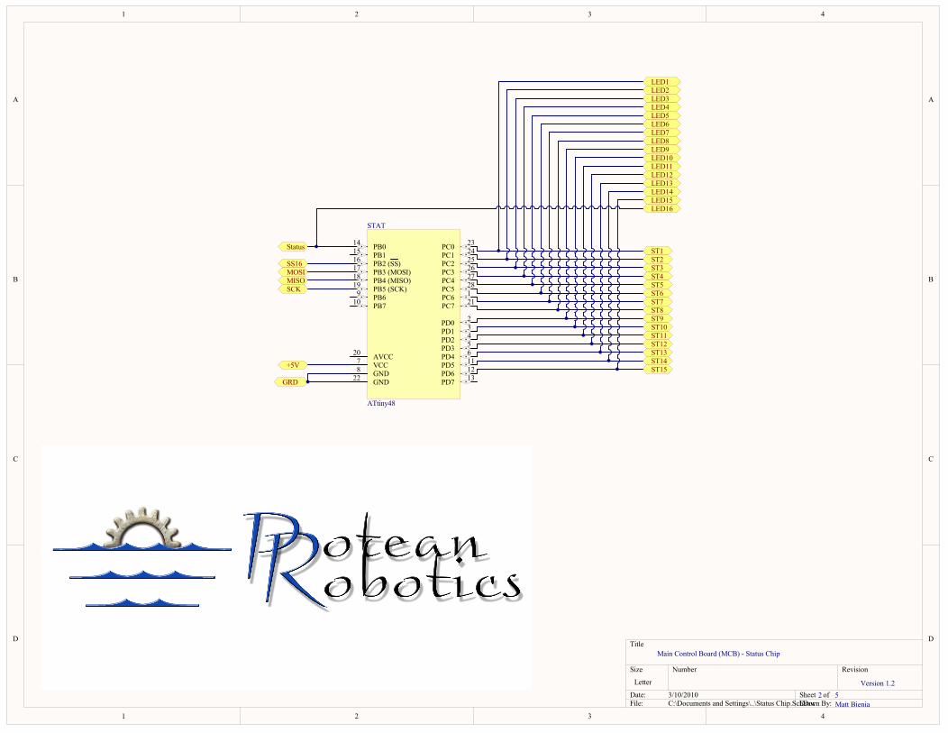
1
1
2
2
3
3
4
4
D D
C C
B B
A A
Title
Number RevisionSize
Letter
Date: 3/10/2010 Sheet ofFile: C:\Documents and Settings\..\Status Chip.SchDocDrawn By:
PC6 1
PD0 2
PD1 3
PD2 4
PD3 5
PD4 6
VCC7
GND8
PB69
PB710
PD5 11
PD6 12
PD7 13
PB014
PB115
PB2 (SS)16
PB3 (MOSI)17
PB4 (MISO)18
PB5 (SCK)19
AVCC20
PC7 21
GND22
PC0 23
PC1 24
PC2 25
PC3 26
PC4 27
PC5 28
STAT
ATtiny48
ST1ST2ST3ST4ST5ST6ST7
ST15
ST8ST9ST10ST11ST12ST13ST14
SS16
+5V
Status
MOSIMISOSCK
Main Control Board (MCB) - Status Chip
Version 1.22 5
Matt Bienia
LED1LED2LED3LED4LED5LED6LED7
LED15
LED8LED9LED10LED11LED12LED13LED14
LED16
GRD
PISTAT01
PISTAT02
PISTAT03
PISTAT04
PISTAT05
PISTAT06
PISTAT07
PISTAT08
PISTAT09
PISTAT010
PISTAT011
PISTAT012
PISTAT013
PISTAT014
PISTAT015
PISTAT016
PISTAT017
PISTAT018
PISTAT019
PISTAT020
PISTAT021
PISTAT022
PISTAT023
PISTAT024
PISTAT025
PISTAT026
PISTAT027
PISTAT028
COSTAT
PISTAT028
POLED6
POST6
PISTAT027
POLED5
POST5
PISTAT026
POLED4
POST4
PISTAT025
POLED3
POST3
PISTAT024
POLED2
POST2
PISTAT023
POLED1
POST1
PISTAT021
POLED8
POST8
PISTAT020
PISTAT019POSCKPISTAT018POMISOPISTAT017POMOSIPISTAT016POSS16PISTAT015
PISTAT014
POLED16
POStatus
PISTAT013
PISTAT012
POLED15
POST15PISTAT011
POLED14
POST14
PISTAT010
PISTAT09
PISTAT08
PISTAT022POGRD
PISTAT07PO05VPISTAT06
POLED13
POST13PISTAT05
POLED12
POST12PISTAT04
POLED11
POST11PISTAT03
POLED10
POST10PISTAT02
POLED9
POST9
PISTAT01
POLED7
POST7
PO05V
POGRD
POLED1POLED2POLED3POLED4POLED5POLED6POLED7POLED8POLED9POLED10POLED11POLED12POLED13POLED14POLED15POLED16
POMISOPOMOSI
POSCK
POSS16
POST1POST2POST3POST4POST5POST6POST7POST8POST9POST10POST11POST12POST13POST14POST15
POSTATUS
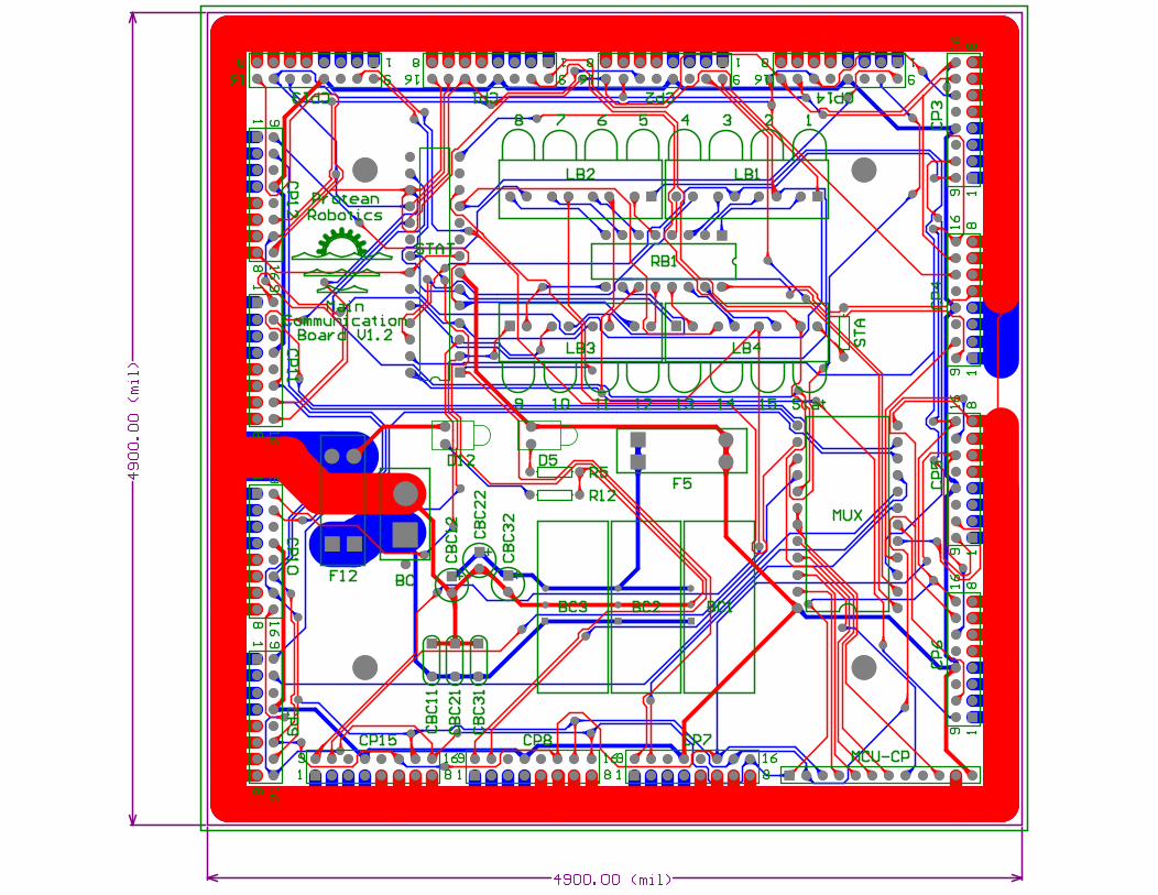
PABC01
PABC02
PABC03COBC
PABC101
PABC103
PABC102 COBC1PABC201
PABC203
PABC202 COBC2PABC301
PABC303
PABC302 COBC3
PACBC1101
PACBC1102
COCBC11
PACBC1202
PACBC1201
COCBC12
PACBC2101
PACBC2102
COCBC21
PACBC2202
PACBC2201
COCBC22
PACBC3101
PACBC3102
COCBC31
PACBC3202
PACBC3201
COCBC32
PACP101PACP102PACP103PACP104PACP105PACP106PACP107PACP108
PACP109PACP1010PACP1011PACP1012PACP1013PACP1014PACP1015PACP1016
COCP1
PACP201PACP202PACP203PACP204PACP205PACP206PACP207PACP208
PACP209PACP2010PACP2011PACP2012PACP2013PACP2014PACP2015PACP2016
COCP2
PACP301
PACP302
PACP303
PACP304
PACP305
PACP306
PACP307
PACP308
PACP309
PACP3010
PACP3011
PACP3012
PACP3013
PACP3014
PACP3015
PACP3016
COCP3
PACP401
PACP402
PACP403
PACP404
PACP405
PACP406
PACP407
PACP408
PACP409
PACP4010
PACP4011
PACP4012
PACP4013
PACP4014
PACP4015
PACP4016
COCP4
PACP501
PACP502
PACP503
PACP504
PACP505
PACP506
PACP507
PACP508
PACP509
PACP5010
PACP5011
PACP5012
PACP5013
PACP5014
PACP5015
PACP5016
COCP5
PACP601
PACP602
PACP603
PACP604
PACP605
PACP606
PACP607
PACP608
PACP609
PACP6010
PACP6011
PACP6012
PACP6013
PACP6014
PACP6015
PACP6016
COCP6
PACP701 PACP702 PACP703 PACP704 PACP705 PACP706 PACP707 PACP708
PACP709 PACP7010 PACP7011 PACP7012 PACP7013 PACP7014 PACP7015 PACP7016
COCP7
PACP801 PACP802 PACP803 PACP804 PACP805 PACP806 PACP807 PACP808
PACP809 PACP8010 PACP8011 PACP8012 PACP8013 PACP8014 PACP8015 PACP8016
COCP8
PACP901
PACP902
PACP903
PACP904
PACP905
PACP906
PACP907
PACP908
PACP909
PACP9010
PACP9011
PACP9012
PACP9013
PACP9014
PACP9015
PACP9016
COCP9
PACP1001
PACP1002
PACP1003
PACP1004
PACP1005
PACP1006
PACP1007
PACP1008
PACP1009
PACP10010
PACP10011
PACP10012
PACP10013
PACP10014
PACP10015
PACP10016
COCP10
PACP1101
PACP1102
PACP1103
PACP1104
PACP1105
PACP1106
PACP1107
PACP1108
PACP1109
PACP11010
PACP11011
PACP11012
PACP11013
PACP11014
PACP11015
PACP11016
COCP11
PACP1201
PACP1202
PACP1203
PACP1204
PACP1205
PACP1206
PACP1207
PACP1208
PACP1209
PACP12010
PACP12011
PACP12012
PACP12013
PACP12014
PACP12015
PACP12016
COCP12
PACP1301PACP1302PACP1303PACP1304PACP1305PACP1306PACP1307PACP1308
PACP1309PACP13010PACP13011PACP13012PACP13013PACP13014PACP13015PACP13016
COCP13
PACP1401PACP1402PACP1403PACP1404PACP1405PACP1406PACP1407PACP1408
PACP1409PACP14010PACP14011PACP14012PACP14013PACP14014PACP14015PACP14016
COCP14
PACP1501 PACP1502 PACP1503 PACP1504 PACP1505 PACP1506 PACP1507 PACP1508
PACP1509 PACP15010 PACP15011 PACP15012 PACP15013 PACP15014 PACP15015 PACP15016
COCP15
PAD502
PAD501
COD5PAD1202
PAD1201
COD12
CODesignator2
PAF501B
PAF502PAF501
PAF502B
COF5
PAF1201B
PAF1202
PAF1201
PAF1202B
COF12
PALB101PALB102PALB103PALB104PALB105PALB106PALB107PALB108
COLB1
PALB201PALB202PALB203PALB204PALB205PALB206PALB207PALB208
COLB2
PALB301 PALB302 PALB303 PALB304 PALB305 PALB306 PALB307 PALB308
COLB3
PALB401 PALB402 PALB403 PALB404 PALB405 PALB406 PALB407 PALB408
COLB4
PAMCU0CP01 PAMCU0CP02 PAMCU0CP03 PAMCU0CP04 PAMCU0CP05 PAMCU0CP06 PAMCU0CP07 PAMCU0CP08 PAMCU0CP09 PAMCU0CP010 PAMCU0CP011 PAMCU0CP012
COMCU0CP
PAMUX024
PAMUX023
PAMUX022
PAMUX021
PAMUX020
PAMUX019
PAMUX018
PAMUX017
PAMUX016
PAMUX015
PAMUX014
PAMUX013 PAMUX012
PAMUX011
PAMUX010
PAMUX09
PAMUX08
PAMUX07
PAMUX06
PAMUX05
PAMUX04
PAMUX03
PAMUX02
PAMUX01
COMUX
PAR501PAR502 COR5
PAR1201PAR1202 COR12
PARB1016PARB1015PARB1014PARB1013PARB1012PARB1011PARB1010PARB109
PARB108 PARB107 PARB106 PARB105 PARB104 PARB103 PARB102 PARB101
CORB1
PASTA01
PASTA02
COSTAPASTAT01
PASTAT02
PASTAT03
PASTAT04
PASTAT05
PASTAT06
PASTAT07
PASTAT08
PASTAT09
PASTAT010
PASTAT011
PASTAT012
PASTAT013
PASTAT014
PASTAT028
PASTAT027
PASTAT026
PASTAT025
PASTAT024
PASTAT023
PASTAT022
PASTAT021
PASTAT020
PASTAT019
PASTAT018
PASTAT017
PASTAT016
PASTAT015
COSTAT
PABC101PABC201PABC301
PABC01
PACBC1102 PACBC2102 PACBC3102
PAF1201PAF1201B
PABC102PABC202PABC302
PABC02
PACBC1101
PACBC1202
PACBC2101
PACBC2202
PACBC3101
PACBC3202
PACP105PACP106PACP107PACP108 PACP205PACP206PACP207PACP208
PACP305
PACP306
PACP307
PACP308
PACP405
PACP406
PACP407
PACP408
PACP505
PACP506
PACP507
PACP508
PACP605
PACP606
PACP607
PACP608
PACP705 PACP706 PACP707 PACP708PACP805 PACP806 PACP807 PACP808
PACP905
PACP906
PACP907
PACP908
PACP1005
PACP1006
PACP1007
PACP1008
PACP1105
PACP1106
PACP1107
PACP1108
PACP1205
PACP1206
PACP1207
PACP1208
PACP1305PACP1306PACP1307PACP1308 PACP1405PACP1406PACP1407PACP1408
PACP1505 PACP1506 PACP1507 PACP1508 PAMCU0CP011
PAMUX012
PAR501
PAR1201
PARB1016
PASTA02
PASTAT08
PASTAT022
PABC103PABC203PABC303PACBC1201
PACBC2201
PACBC3201
PAF501
PAF501B
PACP101PACP102PACP103PACP104 PACP201PACP202PACP203PACP204
PACP301
PACP302
PACP303
PACP304
PACP401
PACP402
PACP403
PACP404
PACP501
PACP502
PACP503
PACP504
PACP601
PACP602
PACP603
PACP604
PACP701 PACP702 PACP703 PACP704PACP801 PACP802 PACP803 PACP804
PACP901
PACP902
PACP903
PACP904
PACP1001
PACP1002
PACP1003
PACP1004
PACP1101
PACP1102
PACP1103
PACP1104
PACP1201
PACP1202
PACP1203
PACP1204
PACP1301PACP1302PACP1303PACP1304 PACP1401PACP1402PACP1403PACP1404
PACP1501 PACP1502 PACP1503 PACP1504
PAD1201
PAF1202PAF1202B
PACP109
PALB101
PASTAT023
PACP1010
PAMUX01
PACP1012 PACP2012
PACP3012
PACP4012
PACP5012
PACP6012
PACP7012PACP8012
PACP9012
PACP10012
PACP11012
PACP12012
PACP13012 PACP14012
PACP15012
PAD501
PAF502
PAF502B
PAMCU0CP012
PAMUX024
PASTAT07
PACP1014 PACP2014
PACP3014
PACP4014
PACP5014
PACP6014
PACP7014PACP8014
PACP9014
PACP10014
PACP11014
PACP12014
PACP13014 PACP14014
PACP15014
PAMCU0CP03
PASTAT019
PACP1015 PACP2015 PACP3015
PACP4015
PACP5015
PACP6015
PACP7015PACP8015PACP9015
PACP10015
PACP11015
PACP12015
PACP13015 PACP14015
PACP15015
PAMCU0CP02
PASTAT018
PACP1016 PACP2016
PACP3016
PACP4016
PACP5016
PACP6016
PACP7016PACP8016
PACP9016
PACP10016
PACP11016
PACP12016
PACP13016 PACP14016
PACP15016
PAMCU0CP01
PASTAT017
PACP209
PALB103
PASTAT024
PACP2010
PAMUX02
PACP309
PALB105
PASTAT025
PACP3010
PAMUX03
PACP409
PALB107
PASTAT026 PACP4010
PAMUX04
PACP509
PALB201
PASTAT027
PACP5010
PAMUX05
PACP609
PALB203
PASTAT028
PACP6010
PAMUX06
PACP709
PALB205
PASTAT01
PACP7010
PAMUX07
PACP809
PALB207
PASTAT021
PACP8010
PAMUX08
PACP909
PALB301
PASTAT02
PACP9010
PAMUX09
PACP1009
PALB303PASTAT03
PACP10010
PAMUX010
PACP1109
PALB305PASTAT04PACP11010
PAMUX011
PACP1209
PALB307
PASTAT05
PACP12010
PAMUX013
PACP1309
PALB401
PASTAT06
PACP13010
PAMUX014
PACP1409
PALB403
PASTAT011
PACP14010
PAMUX015
PACP1509
PALB405
PASTAT012
PACP15010
PAMUX016
PAD502
PAR502
PAD1202
PAR1202
PALB102
PARB101
PALB104
PARB102
PALB106
PARB103
PALB108
PARB104
PALB202
PARB105
PALB204
PARB106
PALB206
PARB107
PALB208
PARB108
PALB302
PARB109
PALB304
PARB1010
PALB306
PARB1011
PALB308
PARB1012
PALB402
PARB1013
PALB404
PARB1014
PALB406
PARB1015
PALB407
PAMCU0CP08
PASTAT014
PALB408
PASTA01
PAMCU0CP04
PAMUX023
PAMCU0CP05
PAMUX022
PAMCU0CP06
PAMUX021
PAMCU0CP07
PAMUX020
PAMCU0CP010
PAMUX018
PAMUX019
PAMUX017
PASTAT016
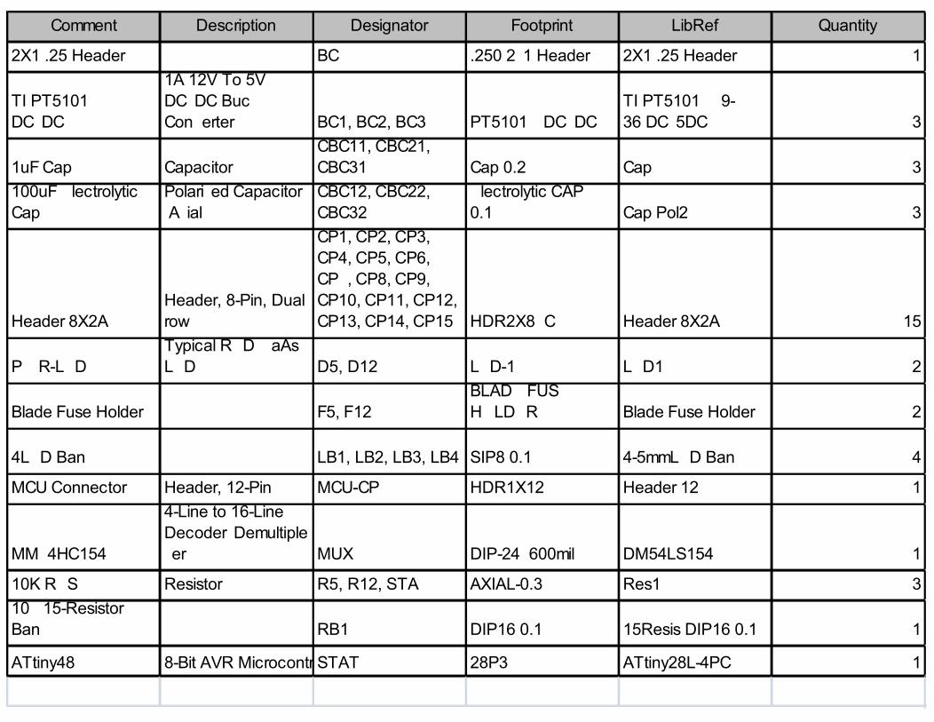
Comment Description Designator Footprint LibRef Quantity
2X1 .25 Header BC .250 2x1 Header 2X1 .25 Header 1
TI PT5101N DC/ DC
1A 12V To 5V DC/ DC Buck Converter BC1, BC2, BC3 PT5101N DC/ DC
TI PT5101N (9-36)DC/ 5DC 3
1uF Cap CapacitorCBC11, CBC21, CBC31 Cap 0.2" Cap 3
100uF Electrolytic Cap
Polarized Capacitor (Axial)
CBC12, CBC22, CBC32
Electrolytic CAP 0.1" Cap Pol2 3
Header 8X2AHeader, 8-Pin, Dual row
CP1, CP2, CP3, CP4, CP5, CP6, CP7, CP8, CP9, CP10, CP11, CP12, CP13, CP14, CP15 HDR2X8_CEN Header 8X2A 15
PWR-LEDTypical RED GaAs LED D5, D12 LED-1 LED1 2
Blade Fuse Holder F5, F12BLADE FUSE HOLDER Blade Fuse Holder 2
4LED Bank LB1, LB2, LB3, LB4 SIP8 0.1" 4-5mmLED Bank 4
MCU Connector Header, 12-Pin MCU-CP HDR1X12 Header 12 1
MM74HC154
4-Line to 16-Line Decoder/ Demultiplexer MUX DIP-24 (600mil) DM54LS154J 1
10K RES Resistor R5, R12, STA AXIAL-0.3 Res1 310k 15-Resistor Bank RB1 DIP16 0.1" 15Resis DIP16 0.1" 1
ATtiny48 8-Bit AVR Microcontroller with 4K Bytes of Flash MemorySTAT 28P3 ATtiny28L-4PC 1

104
7.3. MPU Schematics
(Beginning on the following page)
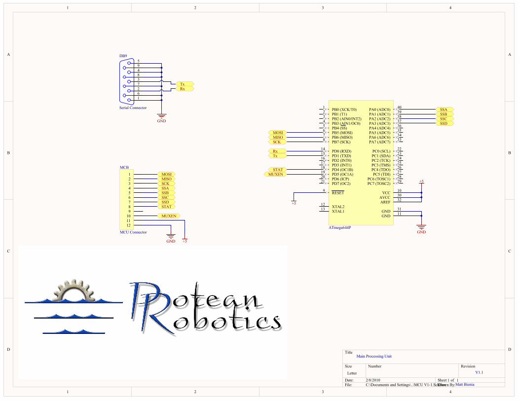
1
1
2
2
3
3
4
4
D D
C C
B B
A A
Title
Number RevisionSize
Letter
Date: 2/8/2010 Sheet ofFile: C:\Documents and Settings\..\MCU V1-1.SchDocDrawn By:
PB0 (XCK/T0)1
PB1 (T1)2
PB2 (AIN0/INT2)3
PB3 (AIN1/OC0)4
PB4 (SS)5
PB5 (MOSI)6
PB6 (MISO)7
PB7 (SCK)8
RESET9
PD0 (RXD)14
PD1 (TXD)15
PD2 (INT0)16
PD3 (INT1)17
PD4 (OC1B)18
PD5 (OC1A)19
PD6 (ICP)20
PD7 (OC2)21
XTAL212
XTAL113
GND 11
PC0 (SCL) 22
PC1 (SDA) 23
PC2 (TCK) 24
PC3 (TMS) 25
PC4 (TDO) 26
PC5 (TDI) 27
PC6 (TOSC1) 28
PC7 (TOSC2) 29
AREF 32AVCC 30
GND 31
PA7 (ADC7) 33PA6 (ADC6) 34PA5 (ADC5) 35PA4 (ADC4) 36PA3 (ADC3) 37PA2 (ADC2) 38PA1 (ADC1) 39PA0 (ADC0) 40
VCC 10
ATmega644P
123456789
101112
MCB
MCU Connector
MOSIMISOSCKSSASSBSSCSSDSTAT
MUXEN
MOSIMISOSCK
SSASSBSSCSSD
STATMUXEN
+5GND
GND
+5
1
2
3
4
5
6
7
8
9
DB9
Serial Connector
GND
RxTx
RxTx
Main Processing Unit
V1.1
1 1Matt Bienia
+5
PIAVR01
PIAVR02
PIAVR03
PIAVR04
PIAVR05
PIAVR06
PIAVR07
PIAVR08
PIAVR09 PIAVR010
PIAVR011
PIAVR012
PIAVR013
PIAVR014
PIAVR015
PIAVR016
PIAVR017
PIAVR018
PIAVR019
PIAVR020
PIAVR021
PIAVR022
PIAVR023
PIAVR024
PIAVR025
PIAVR026
PIAVR027
PIAVR028
PIAVR029
PIAVR030
PIAVR031
PIAVR032
PIAVR033
PIAVR034
PIAVR035
PIAVR036
PIAVR037
PIAVR038
PIAVR039
PIAVR040
COAVRPIDB901
PIDB902
PIDB903
PIDB904
PIDB905
PIDB906
PIDB907
PIDB908
PIDB909
CODB9
PIMCB01
PIMCB02
PIMCB03
PIMCB04
PIMCB05
PIMCB06
PIMCB07
PIMCB08
PIMCB09
PIMCB010
PIMCB011
PIMCB012
COMCB
POMISOPOMOSI
POMUXEN
PORX
POSCK
POSSAPOSSBPOSSCPOSSD
POSTAT
POTX
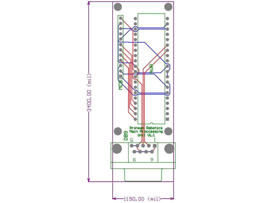
PAAVR01
PAAVR02
PAAVR03
PAAVR04
PAAVR05
PAAVR06
PAAVR07
PAAVR08
PAAVR09
PAAVR010
PAAVR011
PAAVR012
PAAVR013
PAAVR014
PAAVR015
PAAVR016
PAAVR017
PAAVR018
PAAVR019
PAAVR020
PAAVR040
PAAVR039
PAAVR038
PAAVR037
PAAVR036
PAAVR035
PAAVR034
PAAVR033
PAAVR032
PAAVR031
PAAVR030
PAAVR029
PAAVR028
PAAVR027
PAAVR026
PAAVR025
PAAVR024
PAAVR023
PAAVR022
PAAVR021
COAVR
PADB9011 PADB9010PADB901
PADB906
PADB902
PADB907
PADB903
PADB908
PADB904
PADB909
PADB905
CODB9
PAMCB012
PAMCB011
PAMCB010
PAMCB09
PAMCB08
PAMCB07
PAMCB06
PAMCB05
PAMCB04
PAMCB03
PAMCB02
PAMCB01
COMCB
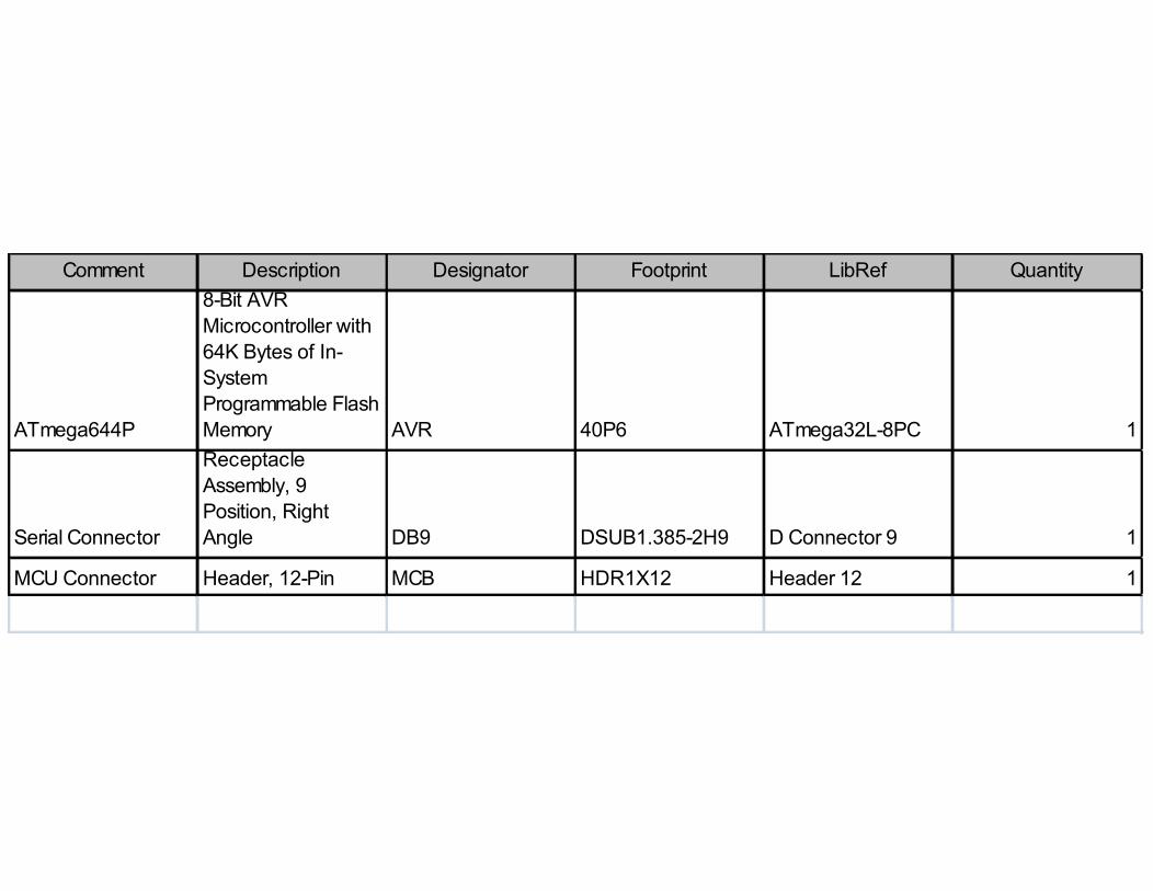
Comment Description Designator Footprint LibRef Quantity
ATmega644P
8-Bit AVR Microcontroller with 64K Bytes of In-System Programmable Flash Memory AVR 40P6 ATmega32L-8PC 1
Serial Connector
Receptacle Assembly, 9 Position, Right Angle DB9 DSUB1.385-2H9 D Connector 9 1
MCU Connector Header, 12-Pin MCB HDR1X12 Header 12 1