Reconsidering Business Cycles of Credit Constraints

Reconsidering Business Cycles of Credit Constraints

─　　─101

Abstract

　　This paper reconsiders the amplification and propagation mechanism of the credit-

constrained economy by highlighting the elasticity of substitution between capital and an asset

used for collateral. We develop a generalized version of the Kiyotaki and Moore (1997, hereafter

KM) model in which capital and land are combined in production with a constant elasticity of

substitution (CES). The substitutability/complementarity between capital and land plays a crucial

role in amplifying quantitative effects of the TFP shock. When the elasticity of substitution is

unity as in the Cobb-Douglas production function, the amplification is small. On the other hand,

when it is small and sufficiently less than unity, credit constraints amplify movements of real

variables. The adjustment cost of investment, combined with the small elasticity of substitution,

strengthens the amplification effect and yields an interesting propagation mechanism among the

holding of land by debtors and investment.

JEL classification number: E32, E44, E23

Keywords: Collateral constraints, Business cycles, Elasticity of substitution, Adjustment cost

跡見学園女子大学マネジメント学部紀要　第 16 号　（2013 年 9 月 10 日）

Reconsidering Business Cycles of Credit Constraints*

Yukie SAKURAGAWA

───────────────────* This work was supported by Overseas Research Program of Atomi University, 2012. We are grateful to Mario Criccini, Kazuo Ogawa, Keiichiro Kobayashi, Shinichi Fukuda, Masaharu Hanazaki, Mototsugu Shintani, Takayuki Tsuruga, Kevin Won, Vu Tuan Khai, Daisuke Miyakawa, and participants of seminars held in Vanderbilt University, Keio University, Asahikawa, Kobe, and development bank of Japan, and the meetings of the Japanese Economic Association and Asia Pacific Economic Association held in Busan University for valuable and insightful comments and discussions.

brought to you by COREView metadata, citation and similar papers at core.ac.uk

https://core.ac.uk/display/229235762?utm_source=pdf&utm_medium=banner&utm_campaign=pdf-decoration-v1

跡見学園女子大学マネジメント学部紀要　第 16 号　2013

─　　─102

1．Introduction

　Ever since Fischer (1933), Kindleberger (1978), and Minsky (1986), huge literature on “credit

channel” and “financial accelerator” has addressed the significant role of the credit channel in

the boom and bust of the aggregate economy. Recently, an increasing literature has applied

credit-constrained models developed by Bernanke and Gertler (1989), Kiyotaki and Moore (1997),

Carlstrom and Fuerst (1997), and Bernanke, Gertler and Gilchrist (1999) to the quantitative

analysis to explain the observed movements of real variables.

　Many researchers have attempted to identify the technology shock as the driving force of

business fluctuations involving credit expansion and contraction, but the existing literature can

only partially explain the observed movements (see, for example, Christiano, Motto and

Rostagno, 2009). Kocherlakota (2000) and Cordoba and Ripoll (2004) added the asset price

channel to the credit-constrained models, but the results are even unsatisfactory.

　One direction of research seems to have taken a turn for identifying shocks that are the

driving force of credit expansion/contraction. Christiano, Eichenbaum and Evans (2005),

Iacoviello (2005), and Christensen and Dib (2008) introduce the monetary shock, and Christiano,

Motto and Rostagno (2009), Jermann and Quardini (2009), and others do the financial shock to

improve the explanation power for the observed variation in real and financial variables.

　Another direction of research is to reconsider the model that explains large amplification

through the channel of borrowers’ balance sheet⑴. The question is whether the existing credit-

constrained models could exploit the transmission mechanism of the interaction between

technology and finance. The behavior of financially-constrained firms that we observe in the

credit boom and bust will be complicated than is supposed. For example, when facing the

appreciation of the asset used as collateral, firms will have a strong motive of “precautionary

saving”, that is, of purchasing the collateralizable asset against the future borrowing limit as

well as purchasing investment goods within the current borrowing limit. The existing models

focus on the balance sheet channel through the asset price change, but are fairly indifferent to

the effect through the change in the distribution of the collateralizable asset between creditors

and debtors.

───────────────────⑴　One direction of modeling is represented by Gertler and Kiyotaki (2011) that incorporate financial

intermediation into the model of financial fractions, where financial intermediaries face the borrowing constraints as well as non-financial borrowers.


─　　─103

　The aim of this paper is to reconsider the transmission mechanism of the credit-constrained

economy by highlighting the interaction between finance and technology captured by the

elasticity of substitution between capital and an asset used for collateral. In particular, we

develop the generalized version of the Kiyotaki and Moore (1997, hereafter KM) model in which

capital and land are combined in production with the constant elasticity of substitution (CES).

　The substitutability/complementarity between capital and land plays a crucial role in

amplifying quantitative effects of the TFP shock. The Cobb-Douglas technology broadly used in

the literature implicitly assumes that entrepreneurs find it easy to substitute capital by other

inputs. Indeed, it is doubtful whether they replace land by capital as quickly as they do labor

by capital. Capital and land are more complementary in production than capital and labor at

least in the short run. The estimation in the Japanese data reports that the elasticity of

substitution is significantly less than unity, supporting the use of the CES-type function with

the small elasticity (see Sakuragawa, 2012).

　We focus on three aspects that interact with the elasticity of substitution in magnifying

movements of real variables. The first is the holding of land by credit-constrained

entrepreneurs, which is determined by the allocation between them and credit-unconstrained

households. When credit-constrained entrepreneurs face the asset price boom, whether they

buy land to increase the future debt capacity or sell land and buy cheaper capital depends on

the elasticity of substitution between capital and land.

　The second is the adjustment cost of investment. When entrepreneurs find it difficult to

invest in capital quickly, they have the motive of buying more land in earlier periods to

enhance the future debt capacity. This precautionary saving of the collateralizable asset

increases the net worth over time and magnifies movements of real variables.

　The third is the adjustment cost of trading land. It will capture the impacts of the liquidity/

illiquidity of the collateralizable asset. Further, the experiment will answer a question if the

adjustment cost and substitutability/complementarity in production have similar or different

implications on the quantitative analysis.

　This paper is related to a number of other works that investigates the quantitative analysis

of the KM model. Kocherlakota (2000), Arias (2003), Cordoba and Ripoll (2004), and Liu, Wang

and Zha (2010) use the standard production technology including the Cobb-Douglas form,

reporting small effects of the technology shock⑵. On the other hand, Iacoviello (2005) reports

significant effects of the monetary and housing preference shocks, and Liu, Wang and Zha

(2010) report significant effects of the collateral and housing preference shocks.


─　　─104

　This paper is related also to the literature that casts doubt on the use of the Cobb-Douglas

technology. Choi and Rios-Rull (2008) study business cycles by focusing on the observed

changeable labor share. Antras (2004) reports that, allowing for biased technological change, the

elasticity of substitution is significantly less than unity in the US aggregate production function.

　This paper is related to the literature that attempts to explain the instability of the credit-

constrained economy. Mendoza (2010) identifies financial crashes followed by severe recessions

of emerging countries by using a nonlinear global approach that deals with both binding and

non-binding credit constraints. Kocherlakota (2010) develops models of land overvaluation by

introducing regulations and/or bubbles.

　This paper is organized as follows. In Section 2 we set up the basic model. In Section 3 we

evaluate the quantitative effects of the developed model. Section 4 concludes.

2．Model

　We consider an economy with one final good, labor, and land. There are two types of

continuum of infinitely-lived patient households and impatient entrepreneurs. The term

“patient/impatient” captures the assumption that impatient agents have a higher subjective

discount rate than patient ones.

　Households consume, work, and demand land for residential use. Entrepreneurs produce the

final good by hiring labor, physical capital, and land. Measures of households and entrepreneurs

are both unity. All markets are perfectly competitive.

A．Households

　Households maximize a lifetime utility given by

(1) 00

[log log ( ) ]tt t t

t

BE c h N

vb fv

where E0 is the expectation operator, b (0, 1) is the discount factor, ct is consumption, ht

denotes the holding of housing, N t is the amount of labor supply, and f, v, and B are positive

───────────────────⑵　Kocherlakota (2000) uses Cobb-Douglas production function that use capital and land, and reports that

the quantitative significance of the amplification is negligible when shares of capital and land sum to less than 40 percent effect, as is approximately true in the U.S. and Japan.


─　　─105

constants. Households lend bt (or borrow bt ) and receive back Rt1bt1, where Rt1 is the real

interest rate on lending between t1 and t. Letting q1 denote the land price, and wt the wage

rate, the flow of funds is

(2) 1 1 1( ) .t t t t t t t t tc q h h w N R b b

Optimum conditions for consumption, housing, and labor are

(3) 1

1 ,ttt t

REc c

b

(4) 1

1,t t

tt t t

q qEc h c

f b and

(5) 1( ) .tt

t

w B Nc

v

B．Entrepreneurs

　Entrepreneurs produce the final good Yt by employing labor Nt , capital Kt1, and land Lt1.

Labor and the “composite capital” are combined with the Cobb-Douglas form, where the

composite capital consists of capital and land, which are combined with the constant elasticity

of substitution (CES). The constant elasticity of substitution between capital and land is

motivated to capture the situation where entrepreneurs will react to the short-run shock by

changing the capital/land ratio less quickly over the business cycle. We consider the following

quasi-CES type technology;

(6) 1 1

1 11 1[ (1 ) ] ,t t t t tY AN K L

s s saa s s sg g

　where At is the total factor productivity (TFP), s is the elasticity of substitution between

capital and land, and g is the weight attached to capital and 1g is the weight attached to land.

A larger s implies greater substitutability. The case for s1 corresponds to the Cobb-Douglas

function, given by . Then ga is the output share of capital and (1g )a is

the output share of land. The case for s0 corresponds to the Leontief technology in which

capital and land are completely complementary⑶.

　Capital evolves as , where It is investment. Following

1 (1 )1 1t t t t tY AN K L a ga g a1 (1 )1 1t t t t tY AN K L a ga g a

1 1(1 ) (1 )t t t t t tK K I K K I d d1 1(1 ) (1 )t t t t t tK K I K K I d d

───────────────────⑶　KM uses the Leontief-type technology that uses capital and land in the same proportion.


─　　─106

Cristiano, Eichenbaum and Evans (2005), the process of transforming investment in equipment

into capital ready for production involves installation and adjustment costs, which increases in

the rate of investment growth, . This form of function is used to

derive the hump-shaped response of investment, which is empirically relevant. Following

Iacoviello (2005), the trade of land may also involve the adjustment cost, a

, due to the market thinness of the land market, regulations, and/or tax

distortion. As studied later, the adjustment cost of trading land measures the liquidity/

illiquidity of the collateralizable asset.

　We assume that there is no enforcement mechanism to fulfill financial contracts between

debtors and creditors. In this society, lenders cannot enforce on borrowers to repay their debt

unless the debts are secured. In order to secure their debt, creditors can only collect land that

the debtor holds⑷. Anticipating the possibility of the borrower’s strategic default, the creditor

limits the amount of credit so that the value of debt will not exceed the value of land that the

borrower holds. Creditors cannot seize capital of their debtors⑸.

　The borrowing constraint that the entrepreneur faces is then typically expressed as

(7) 1( / ),t t t t tb mE q L R

　where m1 is the parameter of the borrowing limit, which is motivated by the notion that

some fraction of the value of land is dissipated in the process of bankruptcy procedure⑹.

　Let the discount factor of entrepreneurs be qb, with q1 so that entrepreneurs are less

patient than households. Entrepreneurs maximize , subject to the technology (6),

the borrowing constraint (7), and the following flow of funds;

(8) 1 1 1 1 1( , ) ( ) ( , , ) .Et t K t t t t t L t t t t t t t t tc I S I I q L L S L q L Y b R b w N

Define ht as the time t shadow value of the borrowing constraint. The first-order conditions for

an optimum are the Euler equation for consumption, the demand functions for labor, land, and

capital:

21

1( , ) ( 1)

2tK

K t t tt

IS I I II

x 2

11

( , ) ( 1)2

tKK t t t

t

IS I I II

x

1 1( , , )L t tS L q L 1 1( , , )L t tS L q L

211

1( )

2t tL

t tt

L L q LL

x 211

1( )

2t tL

t tt

L L q LL

x

0 ( ) lnt EtE c qb0 ( ) lnt EtE c qb

───────────────────⑷　Real estate, such as housing, building, and land, is an asset that has a high liquidation value because it

has many potential buyers across industries (e.g., Shleifer and Vishny, 1992). “Asset liquidity creates debt capacity because liquid assets are in effect better collateral (Shleifer and Vishny, 1992, p.1358)”.

⑸　Almost capital goods do not have well organized secondary markets, and sell for a high discount relative to replacement costs. Ramey and Shapiro (2001) report significant sectoral specificity of physical capital in moving them into new use using equipment-level data in the aerospace industry.

⑹　The bank monitoring may be compatible with the borrowing constraint. Ogawa (2003) reports the evidence of the complementary role of collateral with bank monitoring.


─　　─107

(9) 1

1 ,tt tE E

t t

REc c

qb h

(10) (1 ) ,ttt

YwN

a

(11) , , 11 11

1 1

1 1[ ] [ ] [ ],L t L tt tt t t t tE E

t t t tt t

S Sq Yq m E E qL R L Lc c

h qb and

(12) , , 1 , 221

1 2

1 1 1(1 ) ( ) [ 1 ] ( ) .K t K t K ttt tE E E

t t t tt t t

S S SYE EK K K Kc c c

qb d qb

The demand functions for labor (10) and capital (12) are standard, but the Euler equation for

consumption (9) and the demand function for land (11) are not standard. In each of the latter

two, the multiplier on the borrowing constraint ht is added. In (11) the first term of the RHS

expresses the “down-payment effect” that captures the reduction in the effective land price.

　The assumption q1 guarantees that entrepreneurs are constrained by the borrowing

constraint at least around steady state. In fact, it follows from (3) and (9) that the multiplier is

strictly positive at the steady state; . Therefore, the borrowing constraint will

hold with equality at least around the steady state;

(13) 1 1( / ).t t t tb mE q L R

Finally, we describe the evolutions of the TFP, At , as

(14a) 1ln (1 ) ln ln ,t t tA A A r r e

with et being an observable shock and with the coefficient of autocorrelation r. The value at

the stady-sate of At is denoted by A. Assume that the variance is sufficiently small that the

borrowing constraint is always binding with equality for both positive and negative shocks.

C．Equilibrium

　The equilibrium is a sequence , together with the

sequence of values , satisfying equations (2)-(6), (8)-(13), and four market clearing

conditions, for labor, for land, for loans, and a

for the good, and the sequence of productivity shock (14),

together with the relevant transversally conditions and . To solve the dynamics

numerically, we log-linealize the system around the steady state using the method proposed by

(1 ) 0Ec b qh (1 ) 0Ec b qh

{ } 0, , , , , , , , , ,Et t t t t t t t t t t tY K N N L h c c b b A

{ } 0, , , , , , , , , ,Et t t t t t t t t t t tY K N N L h c c b b A

{ } 0, , ,t t t t tw q R h{ } 0, , ,t t t t tw q R h

t tN N t tN N t th L L t th L L 0t tb b 0t tb b Et t t tY c c K Et t t tY c c K

1 1 , 1(1 ) ( , ) ( , )t K t L t t tK S I I S L q L d 1 1 , 1(1 ) ( , ) ( , )t K t L t t tK S I I S L q L d

{ }1 1 1, ,t t tK L b { }1 1 1, ,t t tK L b


─　　─108

Uhlig (1999).

　Absent shocks, the model has steady state equilibria in which entrepreneurs face the

borrowing constraint. The steady state is described as 10 variables a

, satisfying 10 equations;

(S1) ,h L L

(S2) ,EY c c K d

(S3) 1 ,R b

(S4) (1 ) ,qc h

fb

(S5) ( ) (1 )tB N c Y v a

(S6) 1 1

1 1[ (1 ) ] ,Y AN K L

s s as

a s s sg g

(S7) 1 1 1

1(1 ) ( ), with (1 ) [ (1 ) ] .q Y Yq m R q Y K L LR L L

s ss s sqb qb g a g g

(S8) 1 1 1

11 ( )( 1 ), with [ (1 ) ] .Y Y Y K L KK K

s ss s sqb d ga g g

(S9) / .b mqL R

(S10) (1 ) .Ec K R b Y d a

3．Simulation Results

　In this section we investigate the short-run responses of shocks on macroeconomic

fluctuations.

A．Parameters

　We choose parameter values following the Japanese economy. In the post-war period of

{ , , , , , , , ,Eh L N Y c c K b { , , , , , , , ,Eh L N Y c c K b

},q R},q R


─　　─109

Japan, external finance has been highly dependent on bank loans that were secured by putting

up land as collateral. A number of empirical researches report the important role of the

collateral channel in the financial accelerator, including Ogawa, et al. (1996), Ogawa and

Kitasaka (1998), and Ogawa and Suzuki (1998). Sakuragawa and Sakuragawa (2007) report the

VAR-based response functions of aggregate variables including the land price, finding the

important role of land collateral channel in propagating business fluctuations in Japan. Kwon

(1998) and Bayoumi (2001) argue the important role of land collateral in the monetary

transmission in their VAR analysis.

　The time period is one quarter. We set the discount factor for patient households at b0.995,

which implies the steady-state annualized real interest rate of 2 percent. We set the value of q

at 0.995, implying that the discount factor for entrepreneurs qb to be 0.99. We set parameters

for the labor supply function, B and v to be unity and 1.01. We set the weight for housing at

f0.1. We calculate it by substituting the ratio of expenditure to housing to consumption in

the household sector taken from the National Account into (S4)⑺.

　Next, we consider the value of the elasticity of substitution between capital and land.

According to Sakuragawa (2012), the elasticity from the Japanese annual data is 0.365⑻. The

estimate from the quarterly data would be better because the time period is one quarter in

simulation, but we give up it due to the limitation of the data availability. However, we may

safely judge that the estimate is the upper bound of the real value. We can guess that the

estimate based on the annual data will be greater than the estimate that would be made on the

quarterly data. Then we choose s1/3, and for comparison 1/2, and 1 (the Cobb-Douglas case)

for the elasticity of substitution of land and capital.

　We set the “statistical” capital income share at a0.35, which is the value used in Braun and

Waki (2006), for example. Note that the statistical capital income includes income from both

capital and land, but the parameter g is attributed only to “real” capital. We set g to meet K/Y

4.7, which is the average of the quarterly data for the period 1980-2007, taken from the

National Account. We set g0.85 in case of s1/3.

　We set the entrepreneur’s “loan-to-land-value ratio at m0.7, which reflects the business

───────────────────⑺　Iacoviello (2005) uses the same value for the US economy.⑻　Few researches have estimated the elasticity. Kiyotaki and West (2006) do not estimate but infer the

elasticity to be a little greater than one in their VAR estimation using Japanese aggregate data. Ogawa (2011) estimates the cost function of Japanese manufacturing firms during the bubbly period, and reports that the elasticity between capital and land is far smaller than the one between capital and labor in many industries.


─　　─110

practice and tradition in the Japanese banking industry.

　We set the depreciation rate on capital at d0.02. We set the parameter on the adjustment

cost of investment xK at 0 or 0.5, the value of which is extensively used in the business cycle

literature. The appropriate parameter on the adjustment cost of trading land is difficult to

obtain, and so we use this parameter as a shift parameter. The coefficient of the autocorrelation

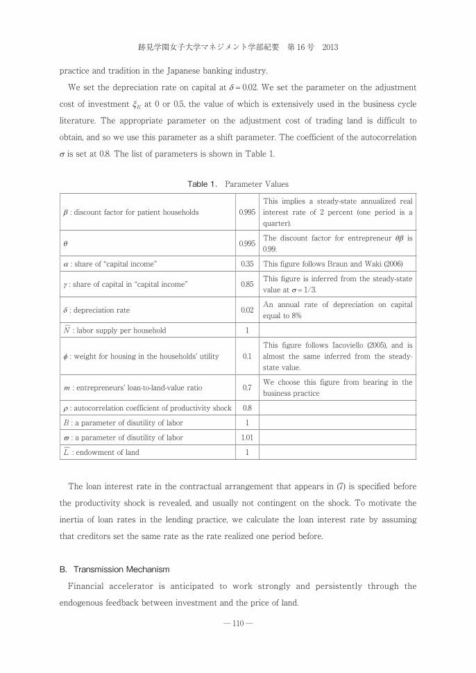
s is set at 0.8. The list of parameters is shown in Table 1.

　The loan interest rate in the contractual arrangement that appears in (7) is specified before

the productivity shock is revealed, and usually not contingent on the shock. To motivate the

inertia of loan rates in the lending practice, we calculate the loan interest rate by assuming

that creditors set the same rate as the rate realized one period before.

B．Transmission Mechanism

　Financial accelerator is anticipated to work strongly and persistently through the

endogenous feedback between investment and the price of land.

Table 1.　Parameter Values

b : discount factor for patient households 0.995This implies a steady-state annualized real interest rate of 2 percent (one period is a quarter).

q 0.995The discount factor for entrepreneur qb is 0.99.

a : share of “capital income” 0.35 This figure follows Braun and Waki (2006)

g : share of capital in “capital income” 0.85This figure is inferred from the steady-state value at s1/3.

d : depreciation rate 0.02An annual rate of depreciation on capital equal to 8%

N─ : labor supply per household 1

f : weight for housing in the households’ utility 0.1This figure follows Iacoviello (2005), and is almost the same inferred from the steady-state value.

m : entrepreneurs’ loan-to-land-value ratio 0.7We choose this figure from hearing in the business practice

r : autocorrelation coefficient of productivity shock 0.8

B : a parameter of disutility of labor 1

v : a parameter of disutility of labor 1.01

L─ : endowment of land 1


─　　─111

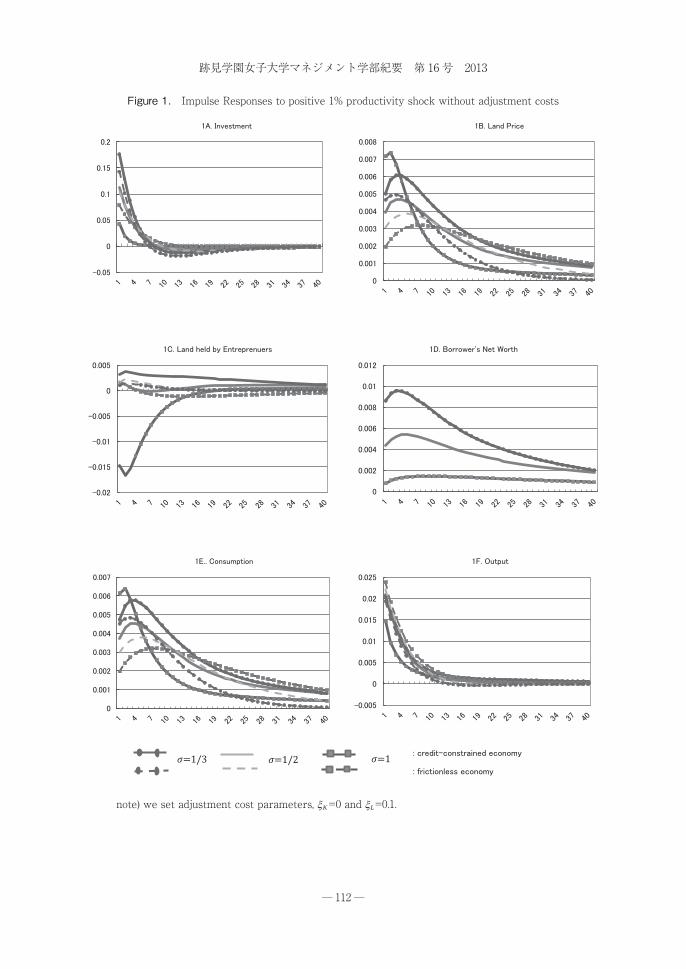
　Figures 1A-E illustrate the effects of a one percent positive technology shock on investment,

the land price, entrepreneurs’ land holding, entrepreneurs’ net worth, consumption, and output.

Entrepreneurs incur neither adjustment cost of investment nor land⑼. Solid impulses represent

the credit-constrained economy, and dotted ones the frictionless economy. The lines with circle,

no marker, and square indicate the response of the economies with s1/3, 1/2 and unity. In

Figure 1A, investment responds more sharply as the elasticity of substitution declines from 1

to 1/2 and to 1/3. Financial friction depresses investment in the Cobb-Douglas case (s1), but

stimulates investment in cases of small elasticity, s1/2 and s1/3.

　In Figure 1B, the land price react more sharply in early periods for all cases, and over the

almost whole periods in cases of s1/2 and s1/3, compared to the frictionless economy.

However, the magnitude of the rise in the price is small even at peak.

　Figure 1C illustrates the impulses of land allocation. Entrepreneurs purchase land in cases of

s1/2 and 1/3, as the steady state analysis has predicted, but sell land in case of s1 . In the

Cobb-Douglas case, entrepreneurs find it easy to substitute land by capital, and choose to sell

land to gain the cash flow to finance investment in capital in the transition. By contrast, in

cases of s1/2 and 1/3, entrepreneurs find it difficult to substitute land by capital, and rather

choose to hold and buy land to serve as collateral.

　In Figure 1D, entrepreneurs’ net worth reacts less for s1, but more for s1/2, and even

more for 1/3. The impulses of net worth reflect the land holding of entrepreneurs more than

the behavior of the land price. Figure 1E illustrates the impulses of consumption, which are

similar to those of the land price⑽. In cases of s1/2 and 1/3, consumption responds more

when there are financial frictions. Figure 1F illustrates the impulses of output. Output reacts

less relative to investment and consumption. In cases of s1/2 and 1/3, investment and

consumption responds more when financial friction exists, but output does not.

　As the elasticity of substitution varies, the quantitative impacts on fluctuations are quite

different when there is financial friction. This experiment suggests that the Cobb-Douglas

function featuring the large elasticity of substitution is the source of the small amplification

effect of the credit-constrained model. In particular, the strength of amplification effect seems

to depend on how the holding of land changes as well as how the price reacts to the shock. In

the small-elasticity cases, the response of the price is moderate, but the holding of land by

entrepreneurs increases (particularly in the case for s1/3), while in the Cobb-Douglas case, ───────────────────⑼　We set the parameter of the adjustment cost of trading land at xL0.1 for MATLAB calculation.⑽　Consumption represents the aggregate consumption of entrepreneurs and households.


─　　─112

note) we set adjustment cost parameters, xK=0 and xL=0.1.

Figure 1.　Impulse Responses to positive 1% productivity shock without adjustment costs


─　　─113

the response of the price is highest at peak, but the holding of land by entrepreneurs decreases.

Consequently, the responses of net worth and thus investment are small.

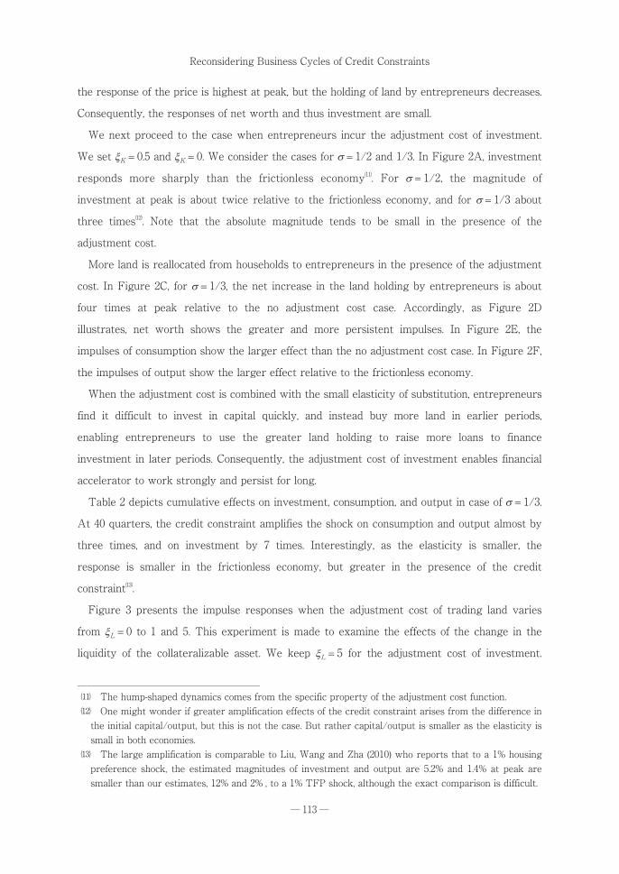
　We next proceed to the case when entrepreneurs incur the adjustment cost of investment.

We set xK0.5 and xK0. We consider the cases for s1/2 and 1/3. In Figure 2A, investment

responds more sharply than the frictionless economy⑾. For s1/2, the magnitude of

investment at peak is about twice relative to the frictionless economy, and for s1/3 about

three times⑿. Note that the absolute magnitude tends to be small in the presence of the

adjustment cost.

　More land is reallocated from households to entrepreneurs in the presence of the adjustment

cost. In Figure 2C, for s1/3, the net increase in the land holding by entrepreneurs is about

four times at peak relative to the no adjustment cost case. Accordingly, as Figure 2D

illustrates, net worth shows the greater and more persistent impulses. In Figure 2E, the

impulses of consumption show the larger effect than the no adjustment cost case. In Figure 2F,

the impulses of output show the larger effect relative to the frictionless economy.

　When the adjustment cost is combined with the small elasticity of substitution, entrepreneurs

find it difficult to invest in capital quickly, and instead buy more land in earlier periods,

enabling entrepreneurs to use the greater land holding to raise more loans to finance

investment in later periods. Consequently, the adjustment cost of investment enables financial

accelerator to work strongly and persist for long.

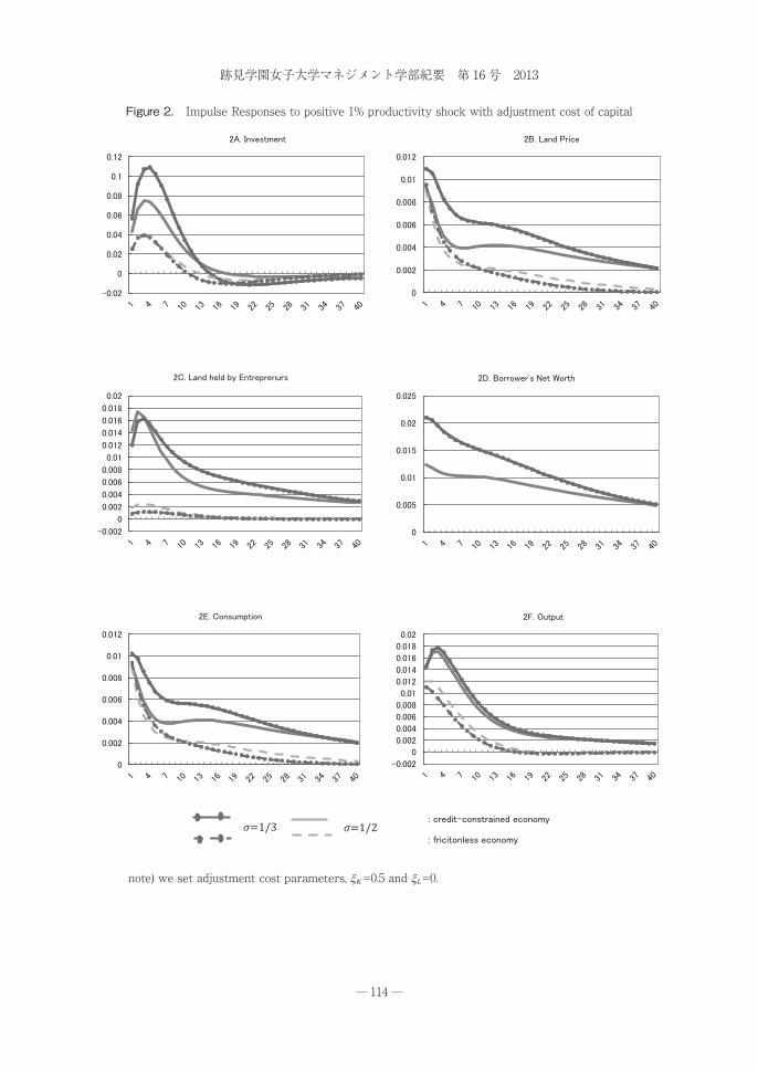
　Table 2 depicts cumulative effects on investment, consumption, and output in case of s1/3.

At 40 quarters, the credit constraint amplifies the shock on consumption and output almost by

three times, and on investment by 7 times. Interestingly, as the elasticity is smaller, the

response is smaller in the frictionless economy, but greater in the presence of the credit

constraint⒀.

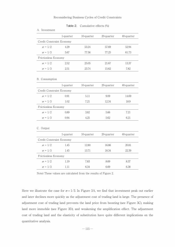
　Figure 3 presents the impulse responses when the adjustment cost of trading land varies

from xL0 to 1 and 5. This experiment is made to examine the effects of the change in the

liquidity of the collateralizable asset. We keep xL5 for the adjustment cost of investment.

───────────────────⑾　The hump-shaped dynamics comes from the specific property of the adjustment cost function.⑿　One might wonder if greater amplification effects of the credit constraint arises from the difference in

the initial capital/output, but this is not the case. But rather capital/output is smaller as the elasticity is small in both economies.

⒀　The large amplification is comparable to Liu, Wang and Zha (2010) who reports that to a 1% housing preference shock, the estimated magnitudes of investment and output are 5.2% and 1.4% at peak are smaller than our estimates, 12% and 2% , to a 1% TFP shock, although the exact comparison is difficult.


─　　─114

note) we set adjustment cost parameters, xK=0.5 and xL=0.

Figure 2.　Impulse Responses to positive 1% productivity shock with adjustment cost of capital


─　　─115

Here we illustrate the case for s1/3. In Figure 3A, we find that investment peak out earlier

and later declines more quickly as the adjustment cost of trading land is large. The presence of

adjustment cost of trading land prevents the land price from boosting (see Figure 3C), making

land more immobile (see Figure 3D), and weakening the amplification effect. The adjustment

cost of trading land and the elasticity of substitution have quite different implications on the

quantitative analysis.

Table 2.　Cumulative effects (%)A. Investment

1-quarter 10-quarter 20-quarter 40-quarter

Credit Constraint Economy

s = 1/2 4.29 53.24 57.69 52.94

s = 1/3 5.67 77.56 77.25 61.73

Frictionless Economy

s = 1/2 2.52 25.05 21.67 13.37

s = 1/3 2.51 23.74 15.62 7.82

B. Consumption



s = 1/2 0.91 5.11 9.09 14.69

s = 1/3 1.02 7.21 12.34 18.9


s = 1/2 0.89 3.82 5.66 7.21

s = 1/3 0.94 4.25 5.62 6.21

C. Output



s = 1/2 1.45 12.80 16.86 20.81

s = 1/3 1.45 13.71 18.34 22.39


s = 1/2 1.19 7.83 8.69 8.37

s = 1/3 1.11 6.34 6.69 6.38

Note) These values are calculated from the results of Figure 2.


─　　─116

note) we set adjustment cost parameter, xK=0.5.

Figure 3.　Impulse Responses to positive 1% productivity shock for various xL

xL xL xL s


─　　─117

4．Conclusion

　We have reconsidered the amplification and propagation mechanism of the credit-constrained

economy by highlighting the interaction of finance and technology captured by the elasticity of

substitution between capital and land in production. The magnitude of amplification depends on

whether credit-constrained entrepreneurs hold the greater (smaller) amount of land in the

boom (bust), which is in turn determined by the elasticity of substitution.

　The distribution of the collateralizable asset between creditors and debtors will become a

significant channel for the quantitative evaluation of the credit boom and bust. Furthermore,

allowing for various production functions beyond the Cobb-Douglas function may be a direction

of research in the field of the quantitative analysis of macroeconomics⒁.

　Our findings provide a number of implications for economic policies. First, the strong

expansion and contraction of credit arise from the large swing of asset prices in the collateral-

dependent economy. Avoiding economic instability will require establishing an alternative

financial system that does not rely on asset collateral. Second, the impact of enhancing liquidity

of assets that serve for collateral is perverse. Policymakers should take into consideration the

fact that enhancing liquidity magnifies macroeconomic fluctuations in the credit-constrained

economy.

References

Antras, P., 2004, “Is the U.S. aggregate production function Cobb-Douglas? New estimates of the elasticity

of substitution,” Contributions to Macroeconomics, vol. 4, issue 1, article 4.

Arias, A.F., 2003, “Quantitative implications of the credit constraint in the Kiyotaki-Moore (1997) setup,”

Documento CEDE 2003-28, ISSN 1657-7191.

Bayoumi, T., 2001, “The morning after: explaining the slowdown in Japanese growth in the 1990s,” Journal

of International Economics, vol. 53, 241-259.

Bernanke, B. S., and M. Gertler, 1989, “Agency costs, net worth, and business fluctuations,” American

Economic Review, vol. 79, 14-31.

Bernanke, B. S., M. Gertler, and S. Gilchrist, 1999, “The financial accelerator in a quantitative business

───────────────────⒁　Sakuragawa and Sakuragawa (2009) extend KM to the endogenous growth model that involves the

Romer-type production function with externalities, and demonstrate that the credit constraint amplifies movements of real variables under most plausible parameter values.


─　　─118

cycle framework,” in Handbook of Macroeconomics, vol. 1, edited by Taylor J. B. and M. Woodford,

Elsevier Science, ch. 21, 1341-1393.

Braun, A., and Y. Waki, 2006, “Monetary policy during Japan’s Lost Decade,” Japanese Economic Review,

vol. 57, 324-344.

Carlstrom, C. T. and T. S. Fuerst, 1997, “Agency costs, net worth, and business fluctuations: a computable

general equilibrium analysis,” American Economic Review, vol. 87, 893-910.

Choi S. and Rios-Rull J.-V., 2008, “Understanding the dynamics of labor share: the role of noncompetitive

factor prices,” Annals of Economics and Statistics, 2009, 251-278.

Christensen, I., and A. Dib., 2008, “The financial accelerator in an estimated New Keynesian model”,

Review of Economic Dynamics, vol. 11, 155-78.

Christiano, L. J., M. Eichenbaum, and C. L. Evans, 2005, “Nominal rigidities and the dynamic effects of a

shock to monetary policy”, Journal of Political Economy, vol. 113, 1-44.

Christiano, L., R. Motto, and M. Rosagno, 2009, “Financial factors in economic fluctuations,” manuscript,

Northwestern University.

Cordoba, J. C. and M. Ripoll, 2004, “Credit cycles redux,” International Economic Review, vol. 45, 1011-1046.

Davis, M. A., 2009, “The price and quantity of land by legal form of organization in the United States,”

Regional Science and Urban Economics, vol. 39, 350-359.

Dickey, D. A. and W. A. Fuller, 1979, “Distribution of the estimation for autoregressive time series with a

unit root,” Journal of the American Statistical Association, vol. 79, 355-376.

Engle R., and C. Granger, 1987, “Co-integration and error correction: representation, estimation, and

testing,” Econometrica, vol. 55, 251-276.

Fisher, I., 1933, “The debt-deflation theory of Great Depression,” Econometrica, vol. 1, 337-357.

Gertler, M., and N. Kiyotaki, 2010, “Financial intermediation and credit policy in business cycle analysis,” in

Handbook of Monetary Economics, vol. 3A, edited by Friedman, B. M., and M. Woodford, North-

Holland, ch. 11, 547-600.

Hayashi, F., 1990, “Taxes and corporate investment in Japanese manufacturing,” in Productivity Growth in

Japan and the United States, edited by Hulten, C. R., University of Chicago Press, ch. 10, 295-316.

Iacoviello. M., 2005, “House prices, borrowing constraints, and monetary policy in the business cycle”,

American Economic Review, Vol. 95, 739-764.

Jermann, U., and V. Quardini, 2009, “Macroeconomic effects of financial shocks,” NBER Working Paper

No. 15338.

Johansen, S., 1991, “Estimation and hypothesis testing of cointegration vectors in Gaussian vector

autoregressive models,” Econometrica, vol. 59, 1551-1580.


─　　─119

　Johansen, S., 1995, Likelihood-based Inference in Cointegrated Vector Autoregressive Models, Oxford

University Press.

Kindleberger, C, P., 1978, Manias, Panics, and Crashes, A history of Financial Crises, 3ed edition, 1996,

Macmillan.

Kiyotaki, N, and J. Moore, 1997, “Credit cycles”, Journal of Political Economy, vol. 105, 211-248.

Kiyotaki, N., and K.D. West, 1996, “Business fixed investment and the recent business cycle in Japan,” in

NBER Macroeconomics Annual, edited by Bernanke, B., and J. Rotemberg, MIT press, 277-323.

Kiyotaki, N., and K. D. West, 2006, “Land prices and business fixed investment in Japan,” in Long-run

Growth and Short-run Stabilization; essays in memory of Albert Ando, edited by Klein, L. R., Edward

Elgar Pub, ch. 12, 303-336.

Kocherlakota, N. R., 2000, “Creating business cycles through credit constraints, Federal Reserve Bank of

Minneapolis Quarterly Review, Vol. 24, No. 3, 2-10.

Kwon, E., 1998, “Monetary policy, land prices, and collateral effects on economic fluctuations: evidence

from Japan,” Journal of the Japanese and International Economies, vol. 12, 175-203.

Liu, Z., P. Wang, and T. Zha, 2010, “Do credit constraints amplify macroeconomic fluctuations?” Working

paper 2010-1, FRB of Atlanta

MacKinnon J. G., 1996, “Numerical distribution functions for unit root and cointegration tests,” Journal of

Applied Econometrics, vol. 11, 601-618.

MacKinnon J. G., A. A. Haug and L. Michelis, 1999, “Numerical distribution functions of likelihood ratio

tests for cointegration,” Journal of Applied Econometrics, vol. 14, 563-577.

Mendoza, E. G., 2010, “Sudden stops, financial crises, and leverage,” American Economic Review, vol. 100,

1941-1966.

Minsky, H., 1986, Stabilizing an Unstable Economy, Yale University Press.

Ogawa, K, 2003, Daifukyo no Keizai Bunseki (in Japanese), Nippon Keizai Shinbun Sha.

Ogawa, K., 2011, “Why are concavity conditions not satisfied in the cost function? The case of Japanese

manufacturing firms during the bubble period,” Oxford Bulletin of Economics and Statistics, vol. 73,

556-580.

Ogawa, K. and S. Kitasaka, 1998, Sisan Shijyou to Keiki Hendou (in Japanese), Nippon Keizai Shinbun Sha.

Ogawa, K., S. Kitasaka, H. Yamaoka and Y. Iwata, 1996, “Borrowing constraints and the role of land asset

in Japanese corporate investment decision”, Journal of the Japanese and International Economics,

vol. 10, 122-149.

Ogawa, K. and K. Suzuki, 1998, “Land value and corporate investment: evidence from Japanese panel

data”, Journal of the Japanese and International Economics, vol. 12, 232-249.


─　　─120

Phillips, P. C. B. and S. Ouliaris, 1990, “Asymptotic properties of residual based tests for cointegration,”

Econometrica, vol. 58, 165-193.

Phillips, P. C. B. and P. Perron, 1988, “Testing for a unit root in time series regression,” Biometrika, vol. 75,

335-346.

Ramey, V. A., and M. D. Shapiro, 2001, “Displaced capital: a study of aerospace plant closings,” Journal of

Political Economy, vol. 109, 958-992.

Sakuragawa, M., and Y. Sakuragawa, 2007, “Land prices and business fluctuations in Japan (in Japanese),”

Mita Journal of Economics, vol. 100, no. 2, 71(507)-93(529).

Sakuragawa, M., and Y. Sakuragawa, 2009, “Land price, collateral, and economic growth,” The Japanese

Economic Review, vol. 60, No. 4, 473-89.

Sakuragawa, Y., 2012, “Technological Substitution between Capital and land,” Journal of Atomi University

Faculty of Management, vol. 14, pp. 125-140.

Shleifer, A., and R. Vishny, 1992, “Liquidation values and debt capacity: a market equilibrium approach,”

Journal of Finance, vol. 47, 1343-1366.

Uhlig, H., 1999, “A toolkit for analyzing nonlinear dynamic stochastic models easily,” in Marimon and Scot,

eds., Computational Methods for the Study of Dynamic Economics. Oxford University Press, 30-61.

Documents

Reconsidering Business Cycles of Credit Constraints