Embed Size (px)
Citation preview
Reconstructing Ancestral Character States Under Wagner Parsimony
DAVID L. SWOFFORD
Srctrotl of Fuunistic Surveys and Insect Identification,
Illrm~rs Naturul Hutor?/ Survey. Champugn, Illinois 61820
AND
WAYNE P. MADDISON
Museum of Compururive Zoo/o,: Hurvurd Liniversity,
Combridge. Massuchusetts 01_738
Recerved 14 November 1986; revised 11 August 1987
ABSTRACT
The problem of assigning optimal character states to the hypothetical ancestors of an
evolutionary tree under the Wagner parsimony criterion is examined. A proof is provided
for the correctness of Farris’s well-known, but previously unproven, algorithm for solving
this problem. However, the solution is not, in general, unique, and Farris’s method obtains
only a subset (generally only one) of the possible solutions. Algorithms that discover other
solutions and that resolve ambiguities through the imposition of ancillary criteria are
developed and discussed. A method for determining the optimal length of a given tree
without actually assigning character states lo hypothetical ancestors is described.
1. INTRODUCTION
Several numerical methods have been developed for estimating phylo- genetic trees under the principle of maximum parsimony [14]. These methods share the goal of finding minimum-length trees: those that minimize the total amount of evolutionary change needed to explain the variation in a given set of data. In the “Wagner method” for inferring phylogenies, character states are measured on an interval scale and no a priori restrictions are imposed either on the reversibility of character changes or on the number of times in which particular character-state transitions may occur [7, 211. Algorithms that strive to optimize Wagner parsimony have achieved
Please address correspondence to David L. Swofford, Illinois Natural Histoly Survey,
607 E. Peabody Drive, Champaign, Illinois 61820.
MATHEMATICAL BIOSCIENCES 87:199-229 (1987)
OElsevier Science Publishing Co., Inc., 1987 52 Vanderbilt Ave., New York, NY 10017
199
0025-5564/87/$3.50
200 DAVID L. SWOFFORD AND WAYNE P. MADDISON
widespread popularity in phylogenetic analysis, largely because of their presumed freedom from assumptions about the nature of the evolutionary process. We will not address the validity of this presumption here; see Felsenstein [14] and Sober [27] for an interesting discussion on the use of parsimony in phylogenetic analysis.
Farris [7] described an algorithm for assigning optimal character states to each of the hypothetical ancestors (interior nodes) on a tree so as to minimize the tree length under the Wagner parsimony criterion. Since this procedure minimizes the totuf amount of change, it also minimizes the amount of extra change or homoplasy: character-state transitions that occur independently in different regions of the tree (parallelisms) and transitions that reflect a reversal in the evolutionary tendency of a character (reversals). When all characters are fully consistent on a tree (i.e., they can evolve on the tree with no homoplasy), Fan-is’s procedure yields a unique solution: only one possible set of character-state assignments will be optimal for the specified tree topology. However, in the presence of homoplasy, there are often many different sets of character-state assignments that minimize the tree length [l, 12, 20,22,23], only some of which will be found by Farris’s [7] method. If we are interested only in estimating the branching pattern of the tree, this ambiguity poses no particular problem, for any of the optimal solutions minimizes the length required for a given topology, and alternative topologies may be evaluated by comparing their optimized lengths. Fre- quently, however, we are interested not only in the branching pattern but also in the evolutionary hypothesis [9]: a phylogeny coupled with the reconstructed states of the characters in the hypothetical ancestors. This evolutionary hypothesis permits us to interpret branch lengths as minimal amounts of evolutionary change and to make inferences about the evolution
of the characters themselves (e.g., [29]). When multiple, equally parsimonious character-state reconstructions ex-
ist, we must be careful in interpreting any one solution. In this paper, we first describe a method for finding all equally parsimonious reconstructions and then introduce several procedures for reducing the arbitrariness in choosing among them. The implications of these results for actual biological studies will be expanded upon in a subsequent paper.
2. BASIC CONCEPTS
We are given a set of n operational taxonomic units (OTUs) whose phylogenetic relationships are summarized by an evolutionary tree or clado- gram. The tree can be described mathematically (e.g., [16, 171) as a con- nected acyclic graph comprising an ordered pair of sets (I’, E), where I/ is a nonempty, finite set of nodes (vertices) and E is a set of unordered pairs { u, , u, }, u, , u, E V, representing branches (edges). (Because some biologists
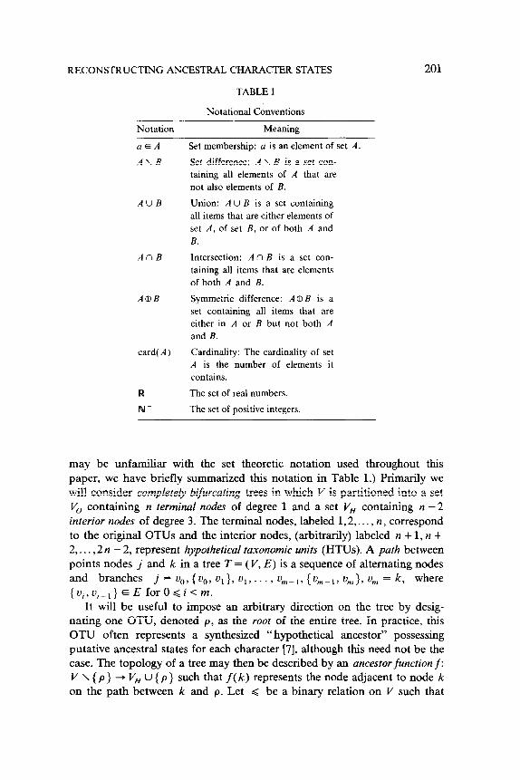
RECONSTRUCTING ANCESTRAL CHARACTER STATES
TABLE 1
Notational Conventions
Notation Meaning
201
UEA
A\B
AUB
AnB
A@B
card(A)
R
Pd+
Set membership: u is an element of set A.
Set difference: A \ B is a set con-
taining all elements of A that are
not also elements of B.
Union: A u B is a set containing
all items that are either elements of
set A, of set B, or of both A and
B.
Intersection: A n B is a set con-
taining all items that are elements
of both A and B.
Symmetric difference: A@ B is a
set containing all items that are
either in A or B but not both A
and B.
Cardinality: The cardinality of set
A is the number of elements it
contains.
The set of real numbers.
The set of positive integers.
may be unfamiliar with the set theoretic notation used throughout this paper, we have briefly summarized this notation in Table 1.) Primarily we will consider completely bifurcating trees in which V is partitioned into a set Vo containing n terminal nodes of degree 1 and a set V, containing n - 2 interior nodes of degree 3. The terminal nodes, labeled 1,2,. . , n, correspond to the original OTUs and the interior nodes, (arbitrarily) labeled n + 1, n +
2,. . . ,2 n - 2, represent hypothetical taxonomic units (HTUs). A path between points nodes j and k in a tree T = (V, E) is a sequence of alternating nodes and branches j = uO, {Q, ul}, ul,. , urn-I, {u,,~~, urn}, u, = k, where
{vi?u,+l }~EforO<i<m.
It will be useful to impose an arbitrary direction on the tree by desig- nating one OTU, denoted p, as the root of the entire tree. In practice, this OTU often represents a synthesized “hypothetical ancestor” possessing putative ancestral states for each character [7], although this need not be the case. The topology of a tree may then be described by an ancestor function f: V \ { p } + V, U { p} such that f(k) represents the node adjacent to node k on the path between k and p. Let Q be a binary relation on V such that
202 DAVID L. SWOFFORD AND WAYNE P. MADDISON
v, Q v, if and only if either v, and v, are coincident or v, lies on the path from v, to p. Since < is reflexive, antisymmetric, and transitive, it repre- sents a partial order on V. The ancestor function f can easily be transformed into the descendant functions g and h. For any interior node k, g(k) and h(k) represent the two immediate descendants, respectively, of k [i.e., f( g( k)) = f( h( k)) = k]. The decision as to which descendant represents g(k) can be made arbitrarily; all results below are invariant to this selection.
We define a subtree T, as the subgraph ( Vk , Ek) of T, where Vk = { v, E
Vlv, Q k} and EL = {{v,,f(v,)} E Elv, < k}. (Biologists refer to a rooted subtree as a monophyletic section of a tree.) A subtree consisting of a single terminal node k, k # p, is called trivial, in which case Ek = 0. The full tree T may then be described as the triple (T,, p, e,,), where 6 represents the interior node adjacent to p (coinciding with the initial bifurcation of the tree) and esP is the basal branch connecting nodes 6 and p. The data consist of a pair (T, X), where T is a tree and X is a rectangular matrix that assigns a character state x,, to each OTU i for each character j. Originally, X is of dimension n by c, where c is the total number of characters. Our task is to assign states for all characters to each of the n - 2 interior nodes (HTUs), augmenting X to (2n -2) X c. A reconstruction on tree T for character j is then given by the pair R(,, = (T,x(,,), where xc,) is a vector con- sisting of the original states x1.,, x2 ,,,. ., x,,, followed by the states X ,1+1,,, X,,+2,,‘,..‘XZn-Z., chosen for the interior nodes. We will denote a reconstruction on the subtree Tk for character j as RCJlk. The length associated with each branch of the tree in this reconstruction is then given by the Manhattan distance D between its incident nodes, where in general
D(k,I) = c h., - %,,I j=l
for any pair of nodes k and 1. The total length L(R) of the reconstruction is simply the sum of the lengths of the branches:
L(R) = c D[i,f(i>] rcv\p
= c c lx,,, - x,c,,,,l iGv\pJ=l
(24
= c c IX!,, - X/(,).,1. (2b)
Note that the equality of statements (2a) and (2b) allows us to treat each character independently; indeed, this independence among characters is a
RECONSTRUCTING ANCESTRAL CHARACTER STATES 203
crucial assumption of the Wagner method. Consequently, to simplify the presentation, we will usually consider only a single character, dropping unnecessary subscripts wherever possible.
In analogy to L(R), the length L(R,) of the reconstruction R, is defined as the sum of the lengths of the 2 nk - 2 branches included in the subtree rooted at k, where nk is the number of terminal nodes in Tk. L*(T) and L*(T,) represent the minimum possible lengths of reconstructions for the tree T and the subtree Tk, respectively. If Tk is trivial, then xk must be assigned the state observed in the data, and both L(R,) and L*(T,) equal zero. A most parsimonious reconstruction (MPR) for tree T is a reconstruc- tion R for which L(R) = L*(T). As noted by Farris [7], when character states take only integer values, the minimum length of a reconstruction can be thought of as the number of steps required by the tree.
In addition to the Manhattan distance function D, we will also refer to the distance d between closed intervals in R, the set of real numbers. Let S,={y(a,<y<b,}=[a,,b,] and S,={yla,<ygbj}=[aj,b,]. The dis- tance between S, and S, is the smallest possible value of ]xi - x,] where x, E S, and x, E S,. This distance can also be written
d(S,,S,)=max(a,-b,,ai-b,,O).
Similarly, the distance between a real number z and an interval S, is defined as the smallest possible value of ]z - xi], where x, E S,:
d(z,S,)=max(z-b;,a,-z,O).
The element of S, closest to z is the median of z, ai, and b,, where a, and b, are greatest lower and least upper bounds, respectively, of S,. Thus, d( z, S, ) can also be computed as
d(z,S,) -It-median(z,aj,bi)).
3. STATE SETS AND FARRIS OPTIMIZATION
Farris’s [7] method for assigning HTU character states so as to obtain the minimum tree length required for a given topology consists of an initial pass during which state sets are computed for all interior nodes on the tree and a final pass in which nonsingleton state sets are replaced by singletons. This procedure has been referred to as “Farris optimization” [25] to distinguish it from “Fitch optimization” [15, 181 in which character states are unordered and any state may transform directly into any other state.
The state set S; is a closed interval in Cp; the smallest and largest elements in this interval place lower and upper bounds, respectively, on the state xi
204 DAVID L. SWOFFORD AND WAYNE P. MADDISON
that will eventually be assigned to an interior node i by Farris’s method. He provides two rules for computing set S, from the state sets of the im- mediately descendant nodes, S,(;, and Shci). The first rule (R-l) dictates that S, = S,(;, I-I S,,(i) if this intersection is not empty. If Sgci) and Shci) are disjoint, Farris’s second rule (R-2) states that S, is the smallest closed interval of the form [a, b] or [b, a], where a E Sgci) and b E Shci).
It will be convenient to define the operator 0 for the “state set operation”: the definition of a state set from two pre-existing state sets according to R-l and R-2. Hereafter, a, and bj will represent the smallest and largest elements, respectively, of the state set S,; that is, S, = { x(ui < x < bi} = [a,, bi]. Farris’s two rules can be expressed jointly as
S,os,=u\(S;@s,),
where U = { x]min( u,, a,) < x < max( b,, b,)}. A convenient computational formula is
S,os,=[min(r,z),max(y,z)l, (3)
where y = median(u,, b,, uj) and z = median( bi, uj, b,). State sets for all nodes on the tree are computed according to the following two steps:
1) For each terminal node i E V, , let S, = { xi }. 2) Visit an interior node k for which Sk has not been defined but for
which the state sets of the two immediate descendants, Sgck) and Shck), have been defined. Compute Sk = Sgck) 0 Shck) using Equation (3). Repeat step 2 until state sets have been assigned to each of the n - 2 interior nodes.
Step 2 is best performed as a postorder traversal of T, (proceeding from the tips of the tree toward the initial bifurcation), ensuring that Sgck) and S,,,, will have been defined prior to consideration of node k. Hereafter, state sets computed in the above manner will be referred to as Furris intervals. Note that the Farris interval calculated for an interior node depends on which OTU was designated p; subsequent redirection of a tree requires a corre- sponding redefinition of its Farris intervals.
After having computed Farris intervals (state sets) for all nodes on the tree steps 1 and 2 above, a final pass over the tree proceeds as follows:
3) For all interior nodes k whose Farris intervals are singleton, let
xk=uk( =bk)
4) Visit an interior node k for which Sk is nonsingleton but for which the state set of its ancestor, S,(k,, is singleton. Let xk equal
median(xf(k)? a,‘, bk). Replace Sk with { xk }. Repeat step 4 until all state sets are singleton.
RECONSTRUCTING ANCESTRAL CHARACTER STATES 205
Step 4 is best performed as a preorder traversal of Tk (proceeding from the initial bifurcation toward the tips), as this ensures that S,Ckj will be singleton prior to consideration of node k.’
Farris’s [7] method was presented without proof. To provide his proce- dure with a more rigorous foundation and to aid in the development and proof of our new algorithms, we now state several useful properties and implications of Farris intervals.
THE BASIC LEMMA
Let TA be a subtree of T rooted at an interior node k. If k’s immediate
ancestor, f(k), is assigned a state x,(~, = y, then
min {Wk)-tl Xk ER
xk-Yl} =L*(T,)+d(Y,S,), (4
where S, is the Farris interval for node k.
Proof. We must show that (a) for any state assignment xk E R to node k,
(5)
(b) there exists at least one reconstruction for Tk such that
L(Rk)+lXk -YI=L*(T,)+d(Y,&). (6)
Let 9 be the set of rooted subtrees contained in Tk such that T,,, E Y iff U, 6 k. Define the poset { .Y, < } where for all T, , To, E .?, T, G T, iff v, < vj. The proof proceeds by induction on the part& order of k. As/ the basis, consider the situation when Tk is trivial, in which case we must assign to node k the corresponding state xk from the data matrix. By definition,
L(R,) = L*(T,) = 0 and Sk = { xk }. Since Sk is singleton, d( y, Sk) = Ixk - y 1, so that Equation (6) is always satisfied.
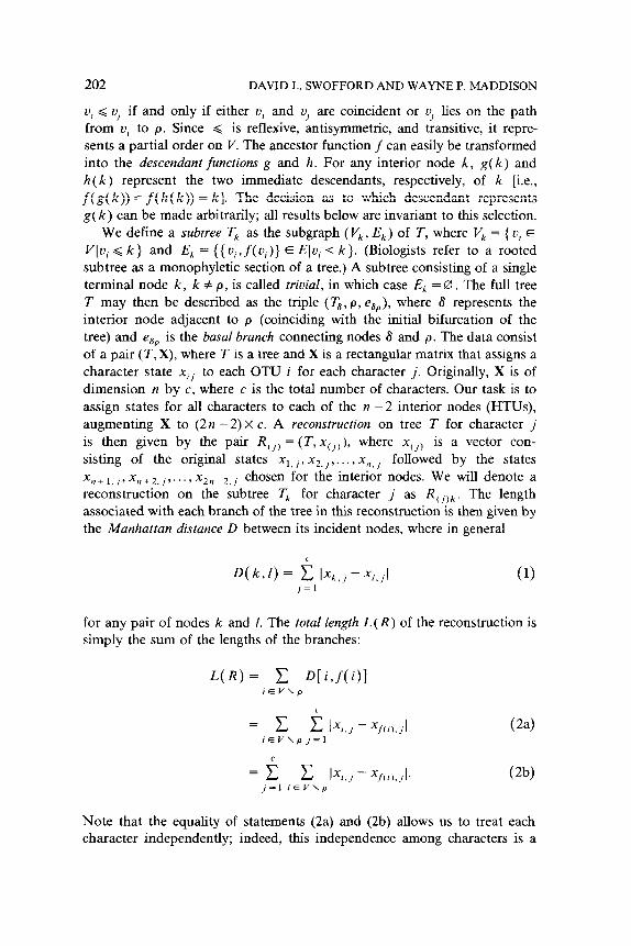
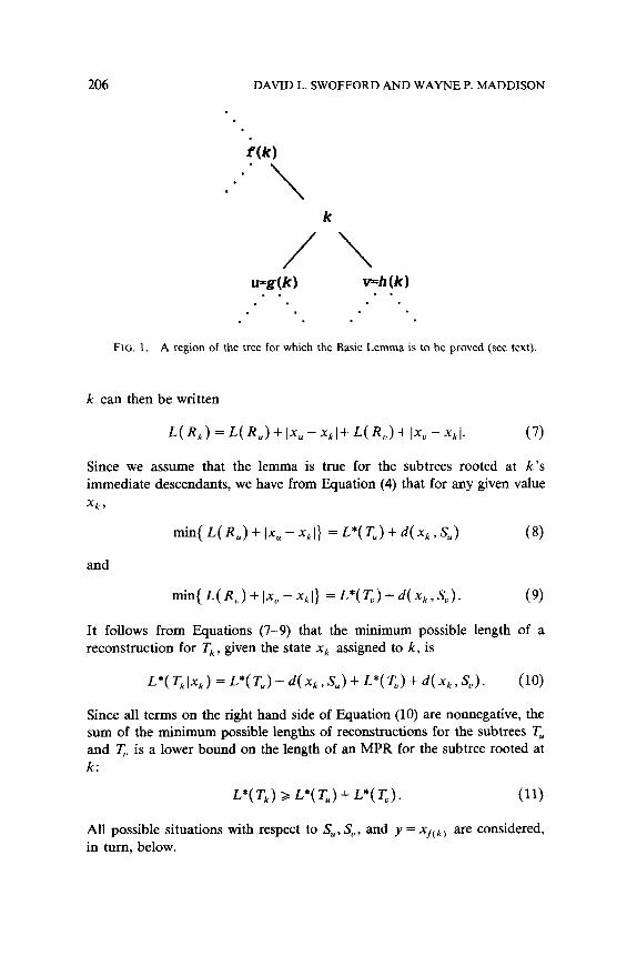
To complete the proof, we must show that Equation (4) is true when k is an interior node, assuming that the lemma holds for TgCkj and ThCkj. Without loss of generality, we can denote nodes g(k) and h(k) as u and v such that a, =G a,. For example, if agCkj <a,,(,), the situation can be depicted graphically as shown in Fig. 1. The length of the subtree rooted at
‘Actually, Farris’s [7] algorithm specifies that for all nodes k having nonsingleton
Farris intervals, xk is obtained as Sk n S,ckj (rule “R-3”). The substitution of our step 4
results in state assignments identical to those obtained using Farris’s rule when Sk n S,ckj
is not empty, but also handles the case that sometimes arises where k = 6 and Sk and S,(k)
are disjoint.
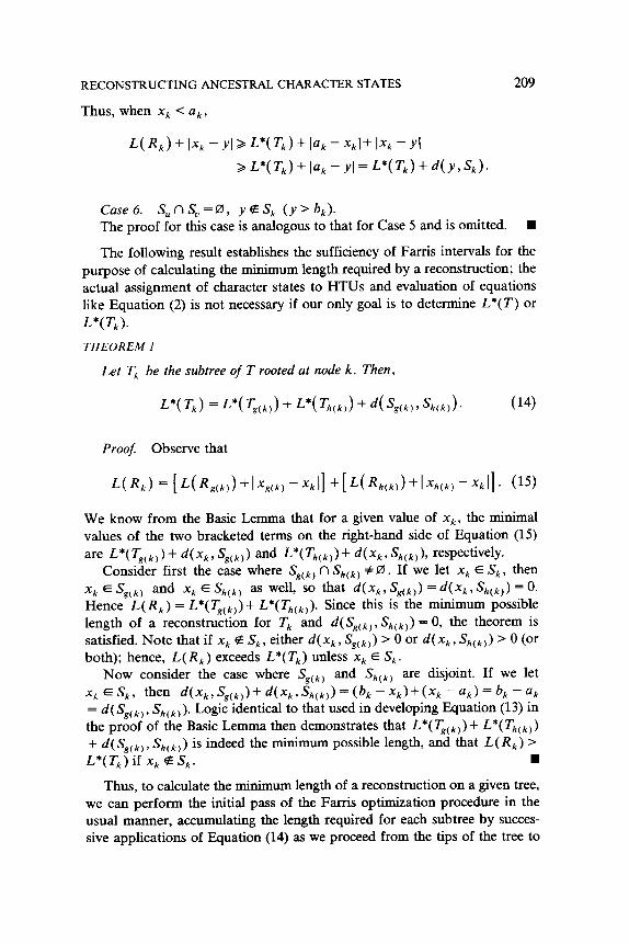
206 DAVID L. SWOFFORD AND WAYNE P. MADDISON
. .
f(k) . . . -\
/*\ u=gW v+(k)
. . . . . * . . . . . . . .
FIG. 1. A region of the tree for which the Basic Lemma is to be proved (see text).
k can then be written
L(h) =L(Ru)+I xu - +I+ L(R) + IX” - %I. (7)
Since we assume that the lemma is true for the subtrees rooted at k’s immediate descendants, we have from Equation (4) that for any given value
xh 7
min{ L( R,) + Ix, - xkl} = L*( T,) + d( xk , S,) (8)
and
min{L(RU)+Ix,-x,1} =L*(T,)+d(x,,S,). (9)
It follows from Equations (7-9) that the minimum possible length of a reconstruction for Tk, given the state xk assigned to k, is
L*(T,lx,) =L*(T,)+d(x,,S,)+L*(T,)+d(x,,S,). (10)
Since all terms on the right hand side of Equation (10) are nonnegative, the sum of the minimum possible lengths of reconstructions for the subtrees T, and q, is a lower bound on the length of an MPR for the subtree rooted at k:
L*(T,) >L*(T,)+L*(T,). (11)
All possible situations with respect to S,,, S,, and y = x,(~, are considered, in turn, below.
RECONSTRUCTING ANCESTRAL CHARACTER STATES 207
Cusel. S,nS,#0, YES,. Let xk = y. Observe that xk E Sk, Sk G S, and Sk c S,; hence, d( xk , S,)
= d(x,, S,) = 0. Then from Equation (lo), L*(T,lx, = y) = L*(T,) + L*(T,), which is the (unconditional) minimum possible length of a recon- struction for Tk[ = L*(T,)]. Since Jxk - yl = d(y, Sk) = 0, Equation (6) is satisfied. If we let xk f y, the minimum value of L( Rk) + (xk - yl exceeds L*(T,)+ d(y, S,), for even if L(R,) = L*(T,), Ixk - yl> 0 = d(y, Sk).
Case2. s,ns,z0, y+ZS, (~<a,). Let xk = ak. Note that ak E Sk, S, 5 S, and Sk c S,; hence d(x,, S,,) =
4-x,, S,) = 0. Then from Equation (lo), L*(Tk(xk = uk) = L*(T,)+ L*(q), which is the (unconditional) minimum possible length of a reconstruction for T, [Inequality (ll)]. Observe that d(y,S,) = uk - y = (xk - yJ, so that Equation (6) is satisfied. To establish Inequality (5) as well, we must show that L( Rk) + (xk - yl can be minimized by letting xk = uk. Suppose instead that we let xk B ak. Even if L( Rk) = L*(T,), xk - y exceeds ak - y, so
that L(R,)+ Ixk - yl> L*(T,)+ (uk - yl. Alternatively, suppose that we let
xk < uk. Note that since uk E [a,,b,]n[a,, b,] and a, 4 a,, uk = a,. Thus,
4x,, S,) = a, - xk = ak - xk = (uk - xkI. Substituting into Equation (10)
and recalling Inequality (ll),
L*(T,lx,<a,)=L*(T,)+d(x,,S,)+L*(~,)+la,-x~I
> L*( T,) + lak - xk(.
Thus, when xk ( a,,
L(h) + lxx -~l~L*(T,)+la,-~~l+l~~-~l.
Applying the triangle inequality,
Case 3. S, n S,, f 0 , y P Sk ( y > b, ). The proof for this case is analogous to that for Case 2 and is omitted.
Case4. s,ns,,=0, ysS,.
Since S, and S,, are disjoint, 4, <b,, < a,, < b,, and Sk = [b,,a,,]. If
Xh ES, then d(x,, S,,) = xk -b, and d(xk,St,)=a,-x,. Then from Equation (lo),
L*(Tklx,~Sk)=L*(Tu)+L*(T,,)+(xk-bu)+(a,-x,)
=L*(T,)+L*(T,)+(a,-b,). (12)
Equation (12) represents the minimum value of L( R,) + Ixk - y 1, subject to
208 DAVID L. SWOFFORD AND WAYNE P. h4ADDISON
xk E Sk, as we can reduce both terms of this expression to their minimum possible (conditional) values by letting xk = y. Since d(y, S,) is then zero, Inequality (5) and Equation (6) are satisfied iff L*(T,Ix, +% Sk) a L*(T,( xk E Sk). Suppose that we let xk < b,. Substituting into Equation (lo),
L*(T,(~,-+,)=L*(T,)+L*(T,)+~(~,,s,)+(~,-x,)
3 L*(T,)+ L*(q,)+(a, -xk)
=L*(T,)+L*(T,)+(a,-b,)+(b,-xk)
>L*(T,)+L*(T,)+(a,,-b,)
=L*(TkIxk=Sk).
Likewise, if we let xk > a,,, then L( Rk) exceeds the value of Equation (12) by at least (xk - a,,). Thus, not only have we established the lemma for this
case, but also we have proven that
L*( Tk) = L*( T,) + L*( T,) +( a, - b,), (13)
when S,nS,,=D and u,,>b,,.
Case5 S,flS,=0, YES, (y<u,). As for Case 4, S, = [b,, a,,]. Let xk = uk( = b,). Then d(x,, S,,) = 0 and
d( xk, s,,) = a,, - xk = u,, - b,. Substituting into Equation (10) and recalling
Equation (13)
L*(TkIxk=uk)=L*(Tu)+L*(q,)+(uU-bU)
= L*(T,).
Observe that d(y, S,) = uk - y = xk - y = Ixk - y(, hence Equation (6) is satisfied. To establish Inequality (5) as well, we must show that L( R, ) + Jxk - yJ can be minimized by letting xk = uk. If instead we let xk > uk, then even if L(R,) = L*(T,), Ixk - yI exceeds d(y, S,) = uk - y.
Alternatively, suppose that we let xk < 0,‘. Then d( xk, s,) = a, - +. Substituting into Equation (lo),
L*(TkIxk<uk) =L*(T,)+L*(T,)+d(X,,&,)+(U,-X,)
> L*( T,) + L*( T,) +( a, - xk)
=L*(T,)+L*(T,)+(u,-b,)+(b,-x,)
=L*(T,)+(b,-x,)=L*(T,)+lu,-x,J
RECONSTRUCTING ANCESTRAL CHARACTER STATES
Thus, when xk < ak,
L(R,) + 1.~ - YI > L*(G) + Ia, - xkl+ 1% -A ~L*(T,)+la,-yl=L*(T,)+d(y,S,).
209
Case6. S,f?S,=0, YES, (y>b,). The proof for this case is analogous to that for Case 5 and is omitted. n
The following result establishes the sufficiency of Farris intervals for the purpose of calculating the minimum length required by a reconstruction; the actual assignment of character states to HTUs and evaluation of equations like Equation (2) is not necessary if our only goal is to determine L*(T) or
L*(T, ).
THEOREM I
Let TA be the subtree of T rooted at node k. Then,
L*(G) =L*(T,(k,)+L*(T,(,,)+d(S,(,,,S,(,,). (14
Proof. Observe that
L(Rk)=~L(R,o,)+IXg(k)-XkI]+[L(Rh(k))+IXh(k)-XkI]. (15)
We know from the Basic Lemma that for a given value of xk, the minimal values of the two bracketed terms on the right-hand side of Equation (15)
are L*(Tgo,)+ d(x,, Sg& and L*(T,,&+ d(xkr+)), respectively. Consider first the case where Sgck) n S,,,,, # 0. If we let xk E S,, then
xh E Sg(k) and xk E h(k) as well, so that d(x,, Sgck,) = d(x,, S,,ckj) = 0. Hence L(R,) = L*(Tgckj)+ L*(Thckj). Since this is the minimum possible length of a reconstruction for Tk and d(S,,,, , Shtkj) = 0, the theorem is satisfied. Note that if xk e Sk, either d(x,, Sgckj) > 0 or d(x,, Sh(kj) > 0 (or both); hence, L(R,) exceeds L*(T,) unless xk E Sk.
Now consider the case where Sg( k) and Shck) are disjoint. If we let
x,, ESk, then d(x,, &(k,> + 4 Xk,Sh(k))=(bk-Xk)+(Xk-ak)=bk-ak
= d&o,, Shckj). Logic identicat to that used in developing Equation (13) in the proof of the Basic Lemma then demonstrates that L*(Tgck,) + L*( Thckj)
+ d(S,(,,, sh,k,) is indeed the minimum possible length, and that L(R,) > L*(T,) if Xk e Sk. n
Thus, to calculate the minimum length of a reconstruction on a given tree, we can perform the initial pass of the Farris optimization procedure in the usual manner, accumulating the length required for each subtree by succes- sive applications of Equation (14) as we proceed from the tips of the tree to
210 DAVID L. SWOFFORD AND WAYNE P. MADDISON
the initial bifurcation. When we arrive at node 6 (the initial bifurcation), we can obtain the minimum length of a reconstruction for the full tree as
L*(T) =L*(~)+d(x,&). (16)
The Basic Lemma guarantees that Equation (16) obtains the minimum value of L(R) = L(R,)+ 1x6 - xp]. Elimination of the final pass saves time when comparing the lengths of alternative tree topologies.
Explicit in the proof of Theorem 1 is the following corollary, which is a generalization of the “root proposition” of Maddison et al. [24]:
COROLLARY 1.1. AN MPR FOR Tk IS POSSIBLE IF AND ONLY IF xk E Sk.
This result establishes that to obtain an MPR for any subtree, it is both necessary and sufficient that the state assignment for the root node of the subtree be selected from the Farris interval computed for that node.
We are now in a position to prove that Farris optimization does indeed obtain an MPR. From the corollary above, we know that an MPR for the subtree T, is possible if xg is chosen from the interval S, as defined during step 2 of the initial pass. Therefore we can obtain an MPR for the full tree by choosing x8 E S, so that the length of the basal branch, Ix8 - xp], is minimized. This length is minimal when x8 = median(x,, as, bs) according to step 4 of the algorithm. [The Basic Lemma guarantees that L(R,)+
1x8 - xp] cannot be reduced further by letting x8 E S,.] Having established that there exists an MPR with x8 chosen according to Farris’s final pass, we now can show by induction that further application of Farris’s method indeed does obtain state assignments that yield an MPR. That is, for any node k, if an MPR exists with f(k) assigned a state x,(~) according to Farris’s final pass, then an MPR also exists with xk assigned according to the algorithm. This induction step follows directly from the Basic Lemma and the fact that choosing xk = median( ak , b, , xrck,) minimizes d( x,(,), S,).
4. MULTIPLE SOLUTIONS
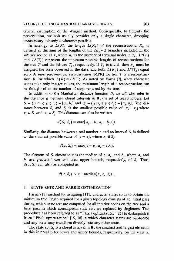
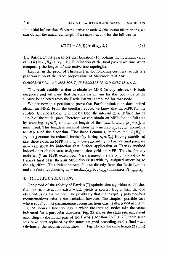
The proof of the validity of Farris’s [7] optimization algorithm establishes that no reconstruction exists which yields a shorter length than the one obtained using his method. The possibility that other equally parsimonious reconstructions exist is not excluded, however. The simplest possible case where equally most parsimonious reconstructions exist is illustrated in Fig. 2. Fig. 2A shows a tree topology in which the terminal nodes take the states indicated for a particular character. Fig. 2B shows the state sets calculated according to the initial pass of the Farris algorithm. In Fig. 2C, these state sets have been replaced by the states assigned according to the final pass. Obviously, the reconstruction shown in Fig. 2D has the same length (2 steps)
RECONSTRUCTING ANCESTRAL CHARACTER STATES 211
A B
(1) (1) (0) 1 2 3
c D I3
O\ 0 0
\ \
/ l\ O\ l\ /l\ / /O\ / /O\
1 1 0 1 1 0 1 1 0
(2 steps) (2 steps) (3 steps)
FIG. 2. An example illustrating the existence of alternative equally most parsimonious
reconstructions. A: States taken by OTUs l-4 are shown in parentheses, node labels in
boldface. B: State sets assigned according to Fanis’s rules. C: Reconstruction obtained
using Farris optimization. D: Another reconstruction requiring the same length as C. E: A
less parsimonious reconstruction,
as that of Fig. 2C. This example makes clear the reason for the failure of Farris’s [7] algorithm to find all MPRs. Although L(R,) is minimal only if x6 = 1 (Corollary l.l), we can permit a less parsimonious reconstruction for T, if the difference can be made up elsewhere, in this case the branch connecting HTU 6 to OTU 4. If the direction of the tree in this example is not arbitrary (i.e., if we have assumed that state 0 is plesiomorphic), the two reconstructions lead to very different interpretations of the mode of evolu- tion of the character: Fig. 2C implies a reversal from state 1 to state 0, whereas Fig. 2D implies parallel transformations from state 0 to state 1. Of course, this is not a novel point; numerous authors have recognized the existence of alternative equally most parsimonious reconstructions (e.g., [l, 2, 6, 12, 20, 221).
212 DAVID L. SWOFFORD AND WAYNE P. MADDISON
Unfortunately, the discovery of equally parsimonious reconstructions is seldom as easy as the example above might indicate, particularly when characters are not binary (0,l). One approach to recognizing the existence of alternative MPRs is to determine, for each interior node k on the tree, the set of states that might be assigned to k in at least one MPR. We will denote this set .Yk and will refer to it informally as k’s MPR-set. If 8 is singleton for all interior nodes i on the tree, the reconstruction is unique. Otherwise, alternative MPRs exist. Faith [6] described an algorithm for discovering “equivocal” character state assignments for binary data (actually a special case of Fitch’s [15] method for unordered multistate characters), but this method does not apply to the general case where characters are measured on an interval scale. Nonetheless, any character with linearly ordered states can be decomposed into a set of additive binary characters that, for our pur- poses, are jointly equivalent to the original single character [13]. Thus we could, at least in principle, use Fitch’s method on the binary-coded data and obtain the MPR-sets for the original character by backtransforming the resulting single-character MPR-sets. However, this approach is both tedious and unnecessary; the methods we describe below apply equally well to binary and (linearly ordered) multistate character data. Furthermore, operat- ing directly on the ordered characters removes a potentially confusing transformation and adds a simpler geometric interpretation, aiding compre-
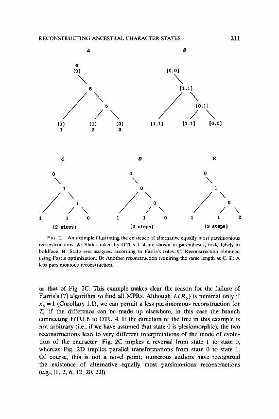
hension of the algorithms. Suppose that we are interested in determining the MPR-set for some
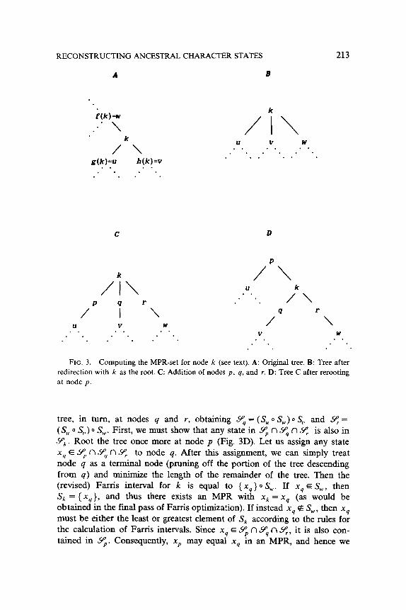
interior node k (Fig. 3A). To simplify the notation to follow, let u = g(k), u = h(k), and w = f( k). We can reroot the tree so that node k is the ancestor of the entire tree, producing a basal trichotomy in the otherwise bifurcating tree (Fig. 3B). Now calculate the Farris intervals S,, S, , and S, by performing the initial pass of Farris optimization on the three subtrees descending from node k. The following result then provides a simple method
for calculating Y;, .
THEOREM .?
The set 9, of states xk that may be assigned to node k in an MPR is
Proof Let us create the new nodes p, q, and r as shown in Fig. 3C. Consider the problem of finding all possible states that might be assigned to node p in an MPR. We can do this by rooting the tree at p (Fig. 3D) and calculating the resulting Farris interval Sp = (S, 0 S,) 0 S,. By Corollary 1.1, S, contains all states that may be assigned to p in at least one MPR (regardless of the tree direction), so that S‘ = Yp. Likewise, we can reroot the
RECONSTRUCTING ANCESTRAL CHARACTER STATES 213
A B
f(k)=w
:. \
/k\
A\ U V W . . . . . . . . . . .
g(k)=u h(k)=v . . . .
. . . . . . I .
. .
C D
A P 4
/ I U V
. * . . . . . .
. .
r
\ W . .
. .
P
/
U
/ V
. .
\ k
/ 9
\ c
\ W . .
. .
FIG. 3. Computing the MPR-set for node k (see text). A: Original tree. B: Tree after
redirection with k as the root. C: Addition of nodes p, q, and r. D: Tree C after rerooting at node p.
tree, in turn, at nodes q and r, obtaining $ = (S, 0 S,,,) 0 S, and 9: = (S, 0 S,,) 0 SW. First, we must show that any state in Yp n Y4 n 9, is also in ~9’~. Root the tree once more at node p (Fig. 3D). Let us assign any state xy E 9, n Yq n Yr to node q. After this assignment, we can simply treat node q as a terminal node (pruning off the portion of the tree descending from q) and minimize the length of the remainder of the tree. Then the (revised) Farris interval for k is equal to { xq } 0 S,,,. If xq E SW, then Sk = ( xq}, and thus there exists an MPR with xk = xq (as would be obtained in the final pass of Farris optimization). If instead xg e S,,,, then xq must be either the least or greatest element of Sk according to the rules for the calculation of Farris intervals. Since xq E $ n 9, n Yr, it is also con-
tained in Yp. Consequently, xp may equal xq in an MPR, and hence we
214 DAVID L. SWOFFORD AND WAYNE P. MADDISON
may also assign xq to node k (again according to the final pass of Farris optimization). Thus any xq E 9” n Y4 fl q can be assigned to k in an MPR.
Next, we must show that any state in Y;, is also in Z$ n 9, n sll,. Consider Fig. 3C. Suppose xk is any element of Yk and we have an MPR with xk, xp, xq, and x, assigned to nodes k, p, q, and r, respectively. The state xk must be the median of xp, xq, and x, [7]. Let us take the case where xp Q xg = xk < x,; other cases can be argued analogously. There exists another MPR having the same state assignments as this one for all nodes other than p and r, but with p and r assigned xk as well (any increase in ]xp - x,] is exactly countered by a decrease in Ix,, - xk] and likewise for
(x, - xk( and Ix, - xw]). Consequently, there exists an MPR with xk as- signed to nodes p, q, r; hence, xk E Yp”,, xk E Yq, and xk E 8. n
By examining all possible cases with respect to the intersection of Yp, Yq, and sPr, we can show that Y;, may also be calculated as follows. Choose a pair of intervals from S,, S,, and S, that are maximally distant (breaking ties arbitrarily). If, for example, d(S,, 5’“) is maximal, then Yk = (S,, 0 S,,) 0 S,,,; calculation of the other two terms in (17) is unnecessary. While recognizing the most distant pair of intervals and applying the appropriate sequence of state set operations is easier for hand computations, application of Theorem 2 is more efficient in computer implementations,
since it avoids the need to evaluate max[ d( S,, , S,), d( S,, S,,,), d( S, , S,,,)] and then branch to separate instructions for computing Yk.
A COMPUTATIONAL ALGORITHM
To obtain the MPR-sets for all interior nodes, we could visit each interior node in turn and appiy Theorem 2 to each. However, this approach would require considerable duplication of effort (in calculating the Farris intervals); the following two-pass algorithm is much more efficient. Note in particular that only the original direction of the tree need be considered; successive rerooting and recomputation of Farris intervals for each rooting is unneces-
sary. The first pass is identical to the initial pass of Farris optimization, visiting
the interior nodes in a postorder traversal. After completing this pass we will have computed the Farris intervals Sk for each of the n - 2 interior nodes k. Then a second pass is performed as follows:
1) Let S{ = ( xp }. Let k = 6. 2) Let SLtkj = Shckj 0 SL and S&k) = Ssckj 0 SL. Note that SL, which will
have been defined in either step 1 or a previous performance of step 2, is equivalent to the Farris interval that would be calculated for node f(k) if the tree had instead been rooted at k.
3) Y;, is then obtained as
~=(Sg(k)~S~~k))n(Sh(k)OSh~k))n(S,oS~).
RECONSTRUCTING ANCESTRAL CHARACTER STATES 215
4) If Sq has been computed for all interior nodes i, stop. Otherwise let k
equal the next interior node in a preorder traversal of the tree and go to 2.
The reader can easily verify that the above procedure is equivalent to successively rerooting the tree at each interior node k and defining yk according to Theorem 2.
5. OBTAINING A RECONSTRUCTION
Although definition of the MPR-sets is useful, these definitions do not lead immediately to a reconstruction unless all of the sets 9’;, are singleton. When ambiguity exists, we cannot freely assign a state xk E Y;, for each node k, as the state assignment made to one node usually places constraints on the states eligible for assignment to other nodes. That these constraints occur is clarified by the example of Fig. 2, where 9s = 9e = [O,l]. For any combination of states y, z E [O,l], there exists at least one MPR where x5 = y and at least one MPR in which xg = z. Yet in this example, xs must equal x6; for instance, we cannot simultaneously let x5 = 0 and x6 =l and still obtain an MPR (Fig. 2E).
Although enumeration of all possible MPRs occasionally may be of interest, it generally will not be feasible, for if the MPR-set for even one interior node is nonsingleton, an infinite number of state assignments could be made. However, if we add the restriction that states assigned to the interior nodes must come from some predefined finite set (e.g., the character states actually observed in the data), we can enumerate all possibilities via a recursive algorithm that recalculates the set of permissible states for each interior node given the state already assigned to its ancestor. By following the implications of every possible assignment at each stage further from the root, we guarantee the discovery of all MPRs.
AN EXAMPLE
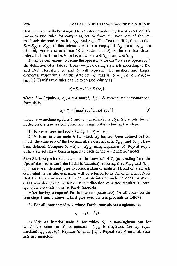
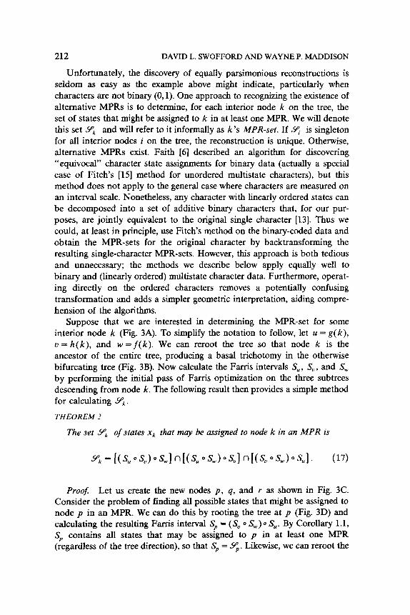
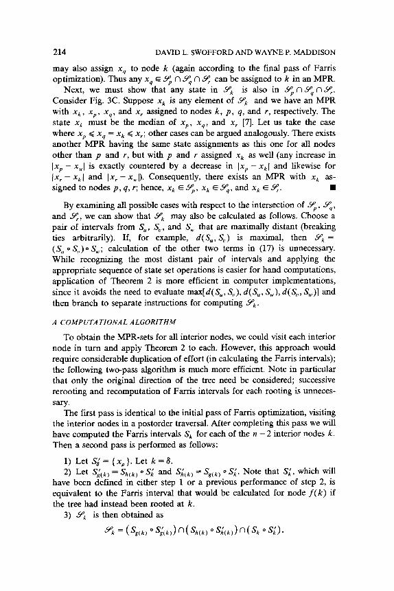
At this point an example will be useful to clarify the points made thus far and to introduce the final segment of the paper. Consider the tree shown in Fig. 4A, where the character states observed in OTUs 1 through 7 take values from the interval [0,6] as indicated. Suppose that we are interested only in determining 9’i,,, the set of states that may be assigned to HTU 10 in at least one MPR. First, we reroot the tree at HTU 10 and compute the
Farris intervals SE, S,, and S,, as [2,4], [5,6], and [l,l], respectively, as shown in Fig. 4B. Using Theorem 2, we calculate the MPR-set for node 10 as
%= KWW~121 Wv~,,>~~,l n[Cv~,,)~~,l
= (1431 o[l,ll> n([I,21 o[5,61) n([l,5]+,4])
= [1,41 n[2,51 n[2,4]
= [2,4].
216
A
DAVID L. SWOFFORD AND WAYNE P. MADDISON
B
A \ 12
/
/lo\ \ T\ /Q\ /ll\ (2) (4) (5) (2) (0) (2) 12345 2
10
/ I \ [2:41
12 (1)
/\/\ /\
(2) (4) (5) (6) (1) 123 4 ‘I z31
/ \
(01 (3) 5 6
FIG. 4. A: Tree topology, node labelings (boldface), and character-state data (in
parentheses) for examples discussed in text. B: Farris intervals after rerooting at HTU 10.
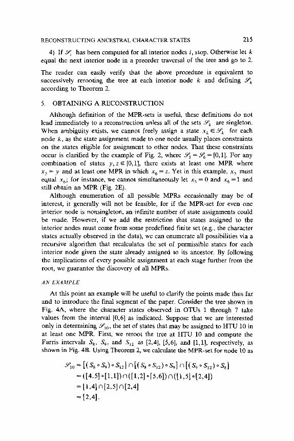
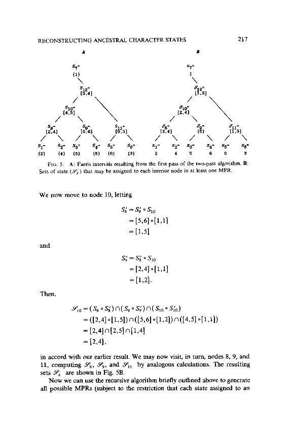
Now suppose we are interested in defining the complete family {Y;, }s G k G 12. We can use the two-pass algorithm for this purpose. The first pass consists of defining the Farris intervals Sk for each interior node k (Fig. 5A). We then let S;, = [l,l] and begin the second pass, first considering node 12.
Following step 2 of the algorithm, we let
S’ g(l2) = &,12, o s;z
s;, = Sll Q s;,
= LO,31 o[Lll
= [1,11
and
S&12, = Sg(12) o siz
s;, = Sl, 0 s;*
= [4,51 o[Lll
= [1,4].
We can now compute YIz as
RECONSTRUCTING ANCESTRAL CHARACTER STATES
A B
%= (1)
\
%2= r3.41
/ %0-
r4.51
/ \ \
X7’ 1
-\ %2= P.31
/
[%
/ \ \
217
IX, Y9- {5)
%= [lo31
/\/\/\ X1’ X2’ X3= X4’ X5’ %’
2 4 5 6 0 3
FIG. 5. A: Farris intervals resulting from the first pass of the two-pass algorithm. B: Sets of state (Y; ) that may be assigned to each interior node in at least one MPR.
We now move to node 10, letting
s,l = s; 0 s,,
= [5,6] +,ll = [1,5]
and
s,l = s,l 0 s,,
= [2,4] #,11 = [1,2].
Then,
sp,o=(~s~~~)n(~,~~~)n(~lo~~~o) = ([2,41~[1,51)n(~5,61~[1~21)~7(~4~51 o[Lll) = [2,4]n[2,5ln[1,41 = t2,4l,
in accord with our earlier result. We may now visit, in turn, nodes 8, 9, and 11, computing A@*, $, and YII by analogous calculations. The resulting sets Yk are shown in Fig. 5B.
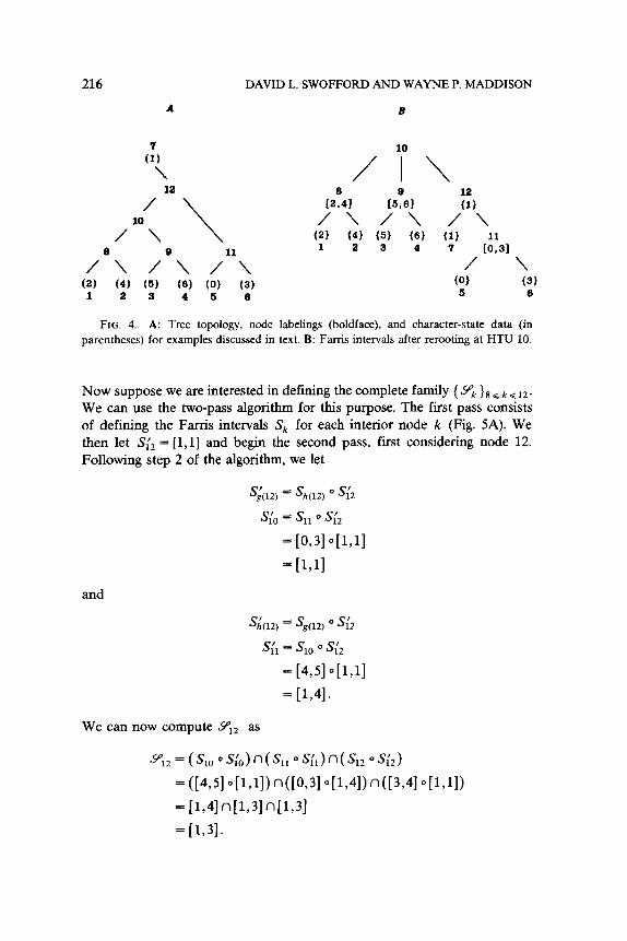
Now we can use the recursive algorithm briefly outlined above to generate all possible MPRs (subject to the restriction that each state assigned to an
218 DAVID L. SWOFFORD AND WAYNE P. h4ADDISON
interior node must be observed in at least one OTU). Initially, we observe that any of the states 1, 2, or 3 may be assigned to node 12. We first let xi1 = 1 and then recalculate the states that may be assigned to nodes 10 and 11, given this assignment. For example, we can temporarily reroot the tree at node k =ll and let u = 5, u = 6, w =12, and Si2 = (1). Substituting into
(17),
%411(X12 =l) =(~0,0]~[3,3])~[1,1]n([0,0]~[1,1])~[3,3]
n([3,31 o[l,ll) o[O,O]
= LO,31 o[l,l] n[0,1] 0[3,3] n[1,3] o[O,O]
= [1,11~[1,3]~[0,1]
= [l,l].
Thus, having made the decision to assign xi2 =l, we must also assign xi, = 1. Now we must consider the possibilities for node 10 given the assignment xi* = 1. Again we temporarily reroot the tree, this time at node k = 10, letting u = 8, u = 9, w = 12, and (as before) S,, = (1). Substituting into (17),
3°K x12 =l) =([2~41~[5,61)~[1,1]n([2,4]~[1,1])~[5,6]
n(W+[L1l)~[2~4l
= [4,5] #,l] n[l,2] 0[5,6] n[l,5] +2,4]
= [1,4] 0[2,5] 0[2,4]
= [2,4].
In this case, no further restrictions were placed on the permissible states for node 10 given that xi* =l. Therefore we must consider, in turn, the
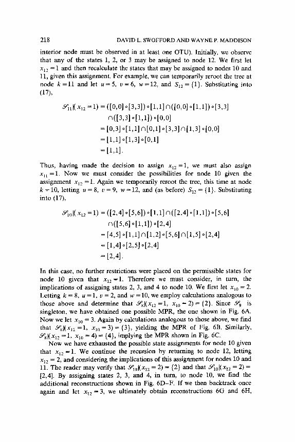
implications of assigning states 2, 3, and 4 to node 10. We first let xi0 = 2. Letting k = 8, u = 1, u = 2, and w = 10, we employ calculations analogous to those above and determine that Ys](xiz = 1, xi0 = 2) = {2}. Since 9s is singleton, we have obtained one possible MPR, the one shown in Fig. 6A. Now we let xi0 = 3. Again by calculations analogous to those above, we find that YK](xii =l, xi0 = 3) = {3}, yielding the MPR of Fig. 6B. Similarly,
%I(%2 = 1, xi0 = 4) = {4}, implying the MPR shown in Fig. 6C. Now we have exhausted the possible state assignments for node 10 given
that xiz = 1. We continue the recursion by returning to node 12, letting xi2 = 2, and considering the implications of this assignment for nodes 10 and 11. The reader may verify that Yii I( xi2 = 2) = { 2) and that Sq, I( xi2 = 2) = [2,4]. By assigning states 2, 3, and 4, in turn, to node 10, we find the additional reconstructions shown in Fig. 6D-F. If we then backtrack once again and let xi2 = 3, we ultimately obtain reconstructions 6G and 6H,
RECONSTRUCTING ANCESTRAL CHARACTER STATES
A B
219
1 1 \ \
1 1 /
/ \ \
/
2 3 / \ \
2 5 1 3 5 1 /\/\/\ / \ / \ / \
2 4 5 6 0 3 2 4 5 6 0 3
C D
1 1 \ \
1 2 /
4 / \ \
/
2 / \ \
4 5 1 2 5 2 /\/\/\ /\I\/\
2 4 5 6 0 3 2 4 5 6 0 3
B P
1 1 \ \
2 2 /
3 / \ \
/
4 / \ \
3 5 2 4 5 2 /\/\/\ /\I\/\
2 4 5 6 0 3 2 4 5 6 0 3
G
1 \
3 /
3 / \ \
3 5 3 /\/\/\
2 4 5 6 0 3
H
1 \
3 /
4 / \ \
4 5 3 / \ / \ / \
2 4 5 6 0 3
FIG. 6. MPRs for example discussed in text.
220 DAVID L. SWOFFORD AND WAYNE P. MADDISON
completing the search for all MPRs under the constraint that all character states assigned to interior nodes are observed in the input data matrix.
6. DEALING WITH AMBIGUITY
Although characters used in actual biological studies are seldom as homoplastic as the one in the example above, a potential dilemma is suggested nonetheless. The example considered a single character, but in real data sets, of course, there will be a number of characters, each of which may yield a nonunique set of optimal character-state assignments. How are we to choose from among the potentially vast array of suitable reconstructions? Several approaches to the resolution of the ambiguity created by the ex- istence of alternative MPRs are described below. The specific method chosen in practical applications will depend ultimately on the investigator’s willing- ness to make assumptions, the nature of the data, and the purpose of the study.
In many studies, certain assumptions regarding the nature of character evolution may be reasonable. For example, the transformation 0 + 1 may seem less probable than the transformation 1 + 0 for a binary character in which 0 means “absence” and 1 means “presence” (i.e., losses are more probable than gains). Thus, for a character such as the one shown in Fig. 2, reconstruction 2C (requiring one 0 +l transformation) would be preferred over that of reconstruction 2D (two 0 + 1 transformations), despite their being “equally parsimonious” in requiring 2 units of change. Evolutionary changes such as those shown in Fig. 2C usually are called reversals, while Fig. 2D exemplifies parallelism. Of course, if the researcher is able to develop a specific model that assigns probabilities to the various events, a maximum likelihood method tailored specifically to these assumptions would provide a better framework for reconstructing ancestral character-state dis- tributions. For certain extreme cases, heuristic alternatives to full maximum likelihood estimation may provide satisfactory results. For example, if the probability of a gain-loss sequence is much greater than the probability of parallel gains, the “Do110 method” [lo], in which multiple gains are expressly
prohibited, may be employed [4]. Similarly, if parallelisms are much more likely than reversals, the method of Camin and Sokal [3], which does not allow reversals, is appropriate.
In most cases, however, alternatives to unrestricted parsimony are inap- propriate or simply not available. The requirement for a meaningful prob- ability model often excludes the use of maximum likelihood methods. Camin-Sokal and Do110 methods may be far too strict in their prohibitions of reversals and parallel gains, respectively. Nonetheless, it may be desirable to use the relative amounts of parallelism and convergence as an ancillary criterion in choosing among competing MPRs. A more complete presenta- tion of this point may be found in Swofford (in preparation).
RECONSTRUCTING ANCESTRAL CHARACTER STATES 221
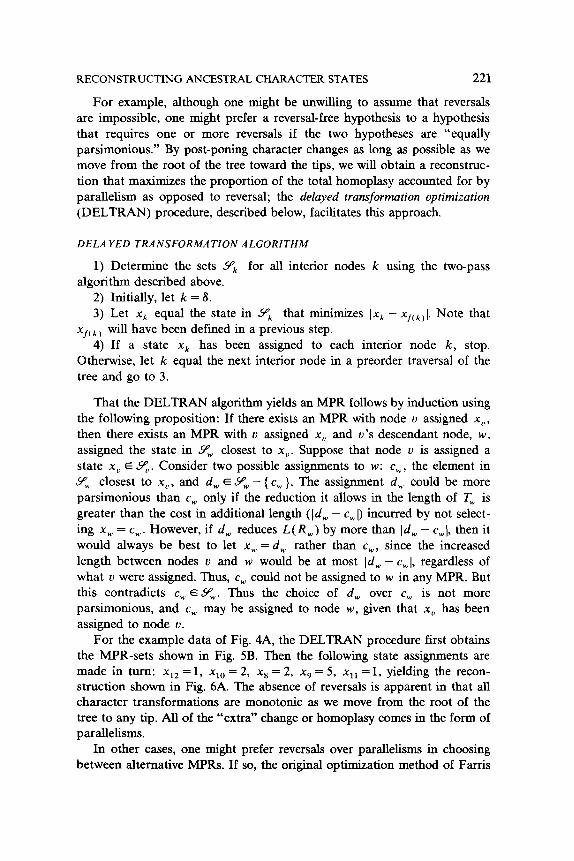
For example, although one might be unwilling to assume that reversals are impossible, one might prefer a reversal-free hypothesis to a hypothesis that requires one or more reversals if the two hypotheses are “equally parsimonious.” By post-poning character changes as long as possible as we move from the root of the tree toward the tips, we will obtain a reconstruc- tion that maximizes the proportion of the total homoplasy accounted for by parallelism as opposed to reversal; the delayed transformation optimization (DELTRAN) procedure, described below, facilitates this approach.
DELAYED TRANSFORMATION ALGORITHM
1) Determine the sets 5$ for all interior nodes k using the two-pass algorithm described above.
2) Initially, let k = 8. 3) Let xk equal the state in Y;, that minimizes Ixk - x,(~,I. Note that
x,( k ) will have been defined in a previous step. 4) If a state xk has been assigned to each interior node k, stop.
Otherwise, let k equal the next interior node in a preorder traversal of the tree and go to 3.
That the DELTRAN algorithm yields an MPR follows by induction using the following proposition: If there exists an MPR with node u assigned x,, then there exists an MPR with v assigned x, and v’s descendant node, w, assigned the state in YW closest to x,. Suppose that node v is assigned a state x,, E q,. Consider two possible assignments to w: c,, the element in Sp,, closest to x,,, and d, E Yw - { c, }. The assignment d, could be more parsimonious than c, only if the reduction it allows in the length of T, is greater than the cost in additional length (Id, - cwD incurred by not select- ing x, = c,. However, if d, reduces L(R,) by more than (d, - c,J, then it would always be best to let x, = d, rather than c,,,, since the increased length between nodes v and w would be at most (d, - c,I, regardless of what v were assigned. Thus, c, could not be assigned to w in any MPR. But this contradicts c, E 9,. Thus the choice of d, over c, is not more parsimonious, and c, may be assigned to node w, given that x, has been assigned to node v.
For the example data of Fig. 4A, the DELTRAN procedure first obtains the MPR-sets shown in Fig. 5B. Then the following state assignments are made in turn: xi2 = 1, xi0 = 2, x8 = 2, x9 = 5, xii = 1, yielding the recon- struction shown in Fig. 6A. The absence of reversals is apparent in that all character transformations are monotonic as we move from the root of the tree to any tip. All of the “extra” change or homoplasy comes in the form of parallelisms.
In other cases, one might prefer reversals over parallelisms in choosing between alternative MPRs. If so, the original optimization method of Farris
222 DAVID L. SWOFFORD AND WAYNE P. h4ADDISON
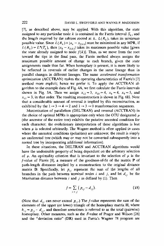
[7], as described above, may be applied. With this algorithm, the state assigned to any particular node k is contained in the Farris interval S, , and the length required by the subtree rooted at k, L(R,), takes its minimum possible value. Since L( Rk) + Ixk - xrck,l must be minimized in any MPR, if
-V&) = L*(q), then IG - x,(~)I takes its maximum possible value [given the state already assigned to node f(k)]. Thus, as we move from the root toward the tips in the final pass, the Farris method always assigns the maximum possible amount of change to each branch, given the state assignments made thus far. When homoplasy is present, it is more likely to be reflected in reversals of earlier changes in the same lineage than in parallel changes in different lineages. The name accelerated transformation
optimization (ACCTRAN) makes the operating characteristics of Farris’s [7] method more explicit; hence we prefer it. To apply the ACCTRAN al- gorithm to the example data of Fig. 4A, we first calculate the Farris intervals shown in Fig. 5A. Then we assign xl2 = 3, xl0 = 4, xs = 4, x9 = 5, and x1, = 3, in that order. The resulting reconstruction is shown in Fig. 6H. Note that a considerable amount of reversal is implied by this reconstruction, as exhibited by the 1 -) 3 + 4 + 2 and 1 + 3 4 0 transformation sequences.
Maximization of parallelism (DELTRAN) and reversal (ACCTRAN) in the choice of optimal MPRs is appropriate only when the OTU designated p (the ancestor of the entire tree) exhibits the putative ancestral condition for each character; the evolutionary interpretation of these algorithms is lost when p is selected arbitrarily. The Wagner method is often applied in cases where the ancestral conditions (polarities) are unknown; the result is simply an undirected tree (which may or may not be converted subsequently into a rooted tree by incorporating additional information).
In these situations, the DELTRAN and ACCTRAN algorithms would have the undesirable property of being dependent on the arbitrary selection of p. An optimality criterion that is invariant to the selection of p is the f-value of Farris [8], a measure of the goodness-of-fit of the matrix P of path-length distances implied by a reconstruction to the original distance matrix D. Specifically, let P,~ represent the sum of the lengths of all branches in the path between terminal nodes i and j, and let djj be the Manhattan distance between i and j as defined by (1). Then
f= C (Pi,-di,). i > j
(18)
(Note that dij can never exceed P,~.) The f-value represents the sum of the elements of the upper (or lower) triangle of the homoplasy matrix H, where h,, = pij - d,,, and therefore sometimes is referred to as the total (pairwise) homoplasy. Other measures, such as the F-value of Prager and Wilson [26] and the “deviation ratio” (DR) used in Fan-is’s Wagner 78 program are
RECONSTRUCTINGANCESTRALCHARACTERSTATES 223
A
(!I t:, cx, (:I
I I I I I I A(O)-0-0-0-1-1-l-(1)H
A(O)-1-1-1-l-1-1-(1)H
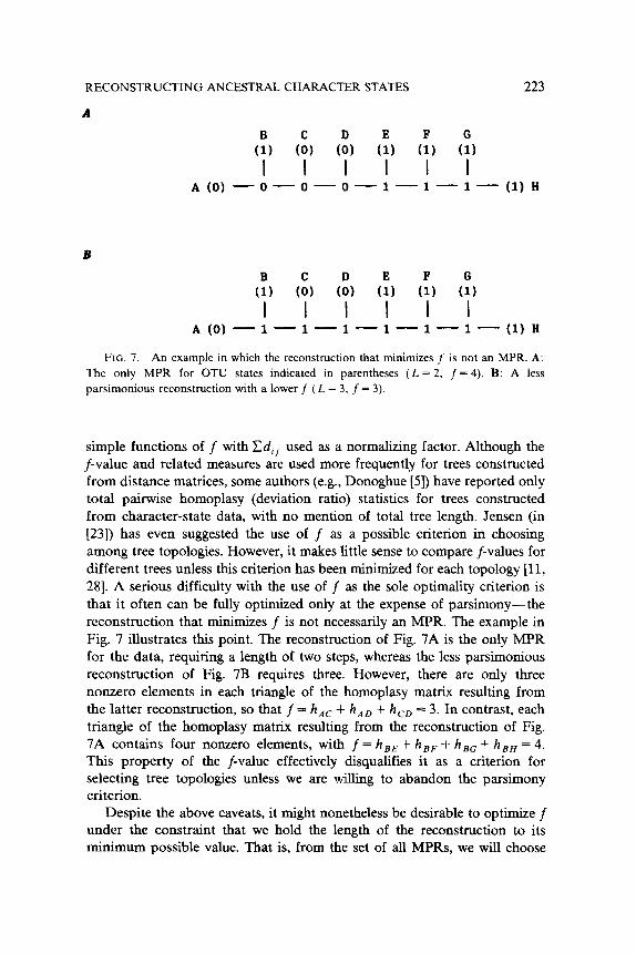
FIG. 7. An example in which the reconstruction that minimizes f is not an MPR. A: The only MPR for OTU states indicated in parentheses (L = 2, f= 4). B: A less parsimonious reconstruction with a lower f (L = 3, f = 3).
simple functions of f with U,, used as a normalizing factor. Although the f-value and related measures are used more frequently for trees constructed from distance matrices, some authors (e.g., Donoghue [5]) have reported only total pairwise homoplasy (deviation ratio) statistics for trees constructed from character-state data, with no mention of total tree length. Jensen (in [23]) has even suggested the use of f as a possible criterion in choosing among tree topologies. However, it makes little sense to compare f-values for different trees unless this criterion has been minimized for each topology [ll, 281. A serious difficulty with the use of f as the sole optimality criterion is that it often can be fully optimized only at the expense of parsimony-the reconstruction that minimizes f is not necessarily an MPR. The example in Fig. 7 illustrates this point. The reconstruction of Fig. 7A is the only MPR for the data, requiring a length of two steps, whereas the less parsimonious reconstruction of Fig. 7B requires three. However, there are only three nonzero elements in each triangle of the homoplasy matrix resulting from the latter reconstruction, so that f = h,, + h,, + h,, = 3. In contrast, each triangle of the homoplasy matrix resulting from the reconstruction of Fig. 7A contains four nonzero elements, with f = h,, + h,, + h,, + h,, = 4. This property of the f-value effectively disqualifies it as a criterion for selecting tree topologies unless we are villing to abandon the parsimony criterion.
Despite the above caveats, it might nonetheless be desirable to optimize f under the constraint that we hold the length of the reconstruction to its minimum possible value. That is, from the set of all MPRs, we will choose
224 DAVID L. SWOFFORD AND WAYNE P. MADDISON
the one(s) with the smallest f. We can rewrite (18) as
f= c P,,- cd.,
i>j i,j 'J'
Since Cd,, is constant for a particular data set, minimizing Cpij is equiv- alent to minimizing f. Furthermore, ZpiJ is simply a weighted function of the branch lengths, where the weights are given by the number of times each branch length is included in the calculation of Cpjj over all distinct pairs of terminal nodes (i, j). Since a branch length is included in the calculation of p,, if and only if it lies on the path between i and j, we can define the weighting function w : E --) WI + as
w(ek) = nk(n - nk),
where e, = (k,f(k)), nk is the total number of OTUs included in k’s subtree ( =l if k is terminal) and n is the total number of OTUs. We will abbreviate w(ek) to wk. An algorithm for finding all MPRs that minimize f (subject to the restriction that states assigned to interior nodes must have been observed in at least one OTU) follows:
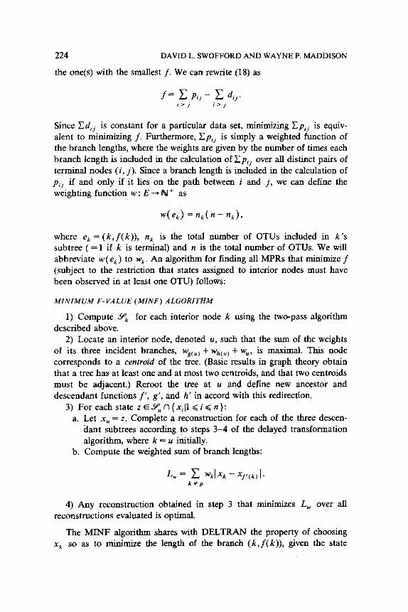
MINIMUM F-VALUE (MINF) ALGORITHM
1) Compute 9” for each interior node k using the two-pass algorithm
described above. 2) Locate an interior node, denoted u, such that the sum of the weights
of its three incident branches, wsc”, + whcu, + w,, is maximal. This node corresponds to a centroid of the tree. (Basic results in graph theory obtain that a tree has at least one and at most two centroids, and that two centroids must be adjacent.) Reroot the tree at u and define new ancestor and descendant functions f’, g’, and h’ in accord with this redirection.
3) ForeachstatezEYun{xill<i<n}: a. Let x, = z. Complete a reconstruction for each of the three descen-
dant subtrees according to steps 3-4 of the delayed transformation algorithm, where k = u initially.
b. Compute the weighted sum of branch lengths:
L= c wklxk-x,~(k)I~ k+p
4) Any reconstruction obtained in step 3 that minimizes L, over all reconstructions evaluated is optimal.
The MINF algorithm shares with DELTRAN the property of choosing xk so as to minimize the length of the branch (k, f( k)), given the state
RECONSTRUCTING ANCESTRAL CHARACTER STATES 225
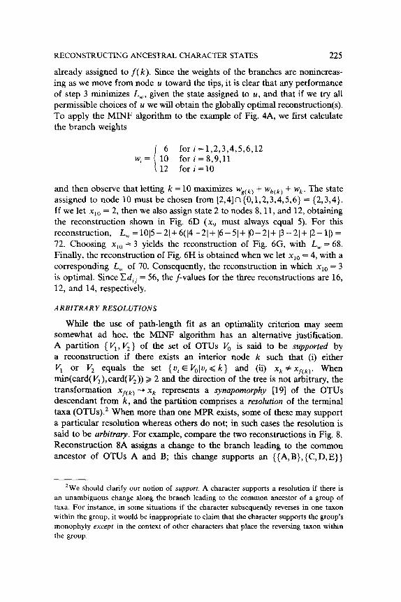
already assigned to f(k). Since the weights of the branches are nonincreas- ing as we move from node u toward the tips, it is clear that any performance of step 3 minimizes L,, given the state assigned to u, and that if we try all permissible choices of u we will obtain the globally optimal reconstruction(s). To apply the MINF algorithm to the example of Fig. 4A, we first calculate the branch weights
i
6 for i =1,2,3,4,5,6,12 w,= 10 fori=8,9,11
12 for i=lO
and then observe that letting k =lO maximizes wgck, + whck, + wk. The state assigned to node 10 must be chosen from [2,4]n{0,1,2,3,4,5,6} = {2,3,4}.
If we let xi0 = 2, then we also assign state 2 to nodes 8,11, and 12, obtaining the reconstruction shown in Fig. 6D (xg must always equal 5). For this reconstruction, L, =1015-2(+6(14-21+ )6-51+ (o-2)+ (3-2)+ 12-11) = 72. Choosing xi0 = 3 yields the reconstruction of Fig. 6G, with L, = 68.
Finally, the reconstruction of Fig. 6H is obtained when we let xi0 = 4, with a corresponding L, of 70. Consequently, the reconstruction in which xi,, = 3 is optimal. Since Cd,, = 56, the f-values for the three reconstructions are 16, 12, and 14, respectively.
ARBITRARY RESOLUTIONS
While the use of path-length fit as an optimality criterion may seem somewhat ad hoc, the MINF algorithm has an alternative justification. A partition { Vi, V, } of the set of OTUs V, is said to be supported by a reconstruction if there exists an interior node k such that (i) either Vi or V, equals the set {ul E VOlvi < k} and (ii) xk + xfck). When min(card( Vi), card( V,)) > 2 and the direction of the tree is not arbitrary, the transformation xrck, -+ xk represents a synupomorphy [19] of the OTUs descendant from k, and the partition comprises a resolution of the terminal taxa (OTUS).~ When more than one MPR exists, some of these may support a particular resolution whereas others do not; in such cases the resolution is said to be arbitrary. For example, compare the two reconstructions in Fig. 8. Reconstruction 8A assigns a change to the branch leading to the common ancestor of OTUs A and B; this change supports an { {A,B}, {C,D,E}}
*We should clarify our notion of support. A character supports a resolution if there is
an unambiguous change along the branch leading to the common ancestor of a group of
taxa. For instance, in some situations if the character subsequently reverses in one taxon
within the group, it would be inappropriate to claim that the character supports the group’s
monophyly except in the context of other characters that place the reversing taxon within
the group.
226 DAVID L. SWOFFORD AND WAYNE P. MADDISON
A B
E E 0 0
0 0 1 1 0 0 1 1 A B c D A B C D
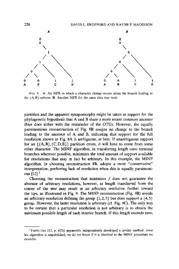
FIG. 8. A: An MPR in which a character change occurs along the branch leading to
the (A.B)-subtree. B: Another MPR for the same data (see text).
partition and the apparent synapomorphy might be taken as support for the phylogenetic hypothesis that A and B share a more recent common ancestor than does either with the remainder of the OTUs. However, the equally parsimonious reconstruction of Fig. 8B assigns no change to the branch leading to the ancestor of A and B, indicating that support for the full resolution shown in Fig. 8A is ambiguous, at best. If unambiguous support for an { {A,B}, {C,D,E}} partition exists, it will have to come from some other character. The MINF algorithm, in transferring length onto terminal branches wherever possible, minimizes the total amount of support available for resolutions that may in fact be arbitrary. In this example, the MINF algorithm, in choosing reconstruction 8B, adopts a more “conservative” interpretation, preferring lack of resolution when this is equally parsimoni- ous [12].3
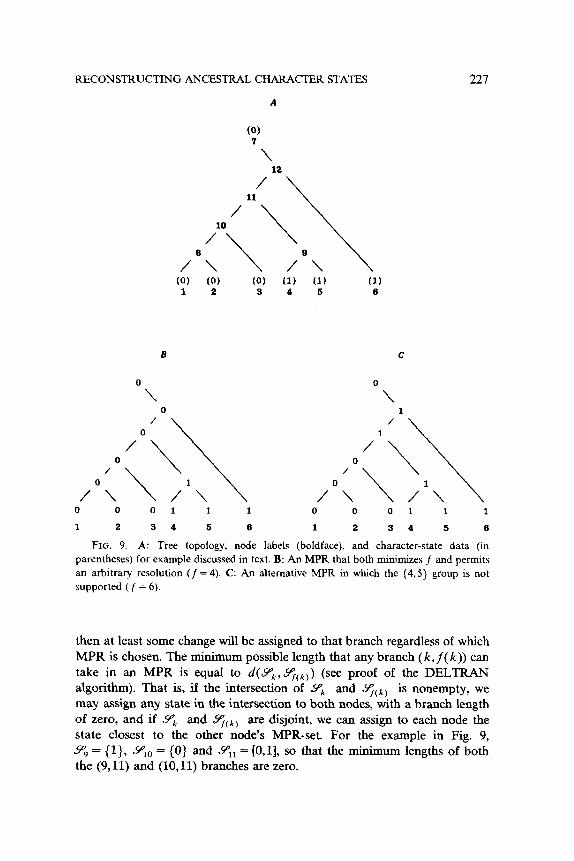
Choosing the reconstruction that minimizes f does not guarantee the absence of arbitrary resolutions, however, as length transferred from the center of the tree may result in an arbitrary resolution further toward the tips, as illustrated in Fig. 9. The MINF reconstruction (Fig. 9B) avoids an arbitrary resolution defining the group {1,2,3} but does support a {4,5} group. However, the latter resolution is arbitrary (cf. Fig. 9C). The only way to be certain that a particular resolution is not arbitrary is to obtain the minimum possible length of each interior branch. If this length exceeds zero,
3Farris (see [12, p. 4251) apparently independently developed a similar method; since
his algorithm is unpublished, we do not know if it is identical to the MINF procedure we
describe.
RECONSTRUCTING ANCESTRAL CHARACTER STATES 227
A
(0)
‘1 12 /
7 /‘“\ \\
A (0) (0) 1 2
\ /Q\ \ (0) (1) (1) (1) 3 4 5 6
B
O\ 0 /
/O 0 \\
C
0
\
/
7 0 \\
/OL\ A\ /Ok\ A\ 0 0 0 1 1 1 0 0 0 1 1 1
1 2 3 4 5 6 1 2 3 4 5 6
FIG. 9. A: Tree topology, node labels (boldface), and character-state data (in
parentheses) for example discussed in text. B: An MPR that both minimizes f and permits
an arbitrary resolution (/ = 4). C: An alternative MPR in which the (4,5} group is not
supported ( f = 6).
then at least some change will be assigned to that branch regardless of which MPR is chosen. The minimum possible length that any branch (k, f( k)) can take in an MPR is equal to d(SP,, qCk)) (see proof of the DELTRAN algorithm). That is, if the intersection of Y;, and qCk) is nonempty, we may assign any state in the intersection to both nodes, with a branch length of zero, and if Y;, and Y;Ck) are disjoint, we can assign to each node the state closest to the other node’s MPR-set. For the example in Fig. 9, 9, = {l}, YIo = (0) and Sq, = [O,l], so that the minimum lengths of both the (9,ll) and (10,ll) branches are zero.
228 DP.VID L. SWOFFORD AND WAYNE P. M4DDISON
The amount of potential support for a given resolution is also of interest. Whenever Yk # 5$( k ), at least one reconstruction will support the resolution, as we can assign to at least one node a state from the symmetric difference of the two MPR-sets. To determine the maximum support available for the resolution, we can calculate the maximum possible length of the branch (k,f( k)) in an MPR by rerooting the tree at a point p between k and f(k) = u and calculating the Farris intervals for k and u after the redirec- tion. From Theorem 1, L*( T,) = L*( Tk) + L*( T,) + d( Sk, S,). It follows that d( Sk, S,,) is the maximum possible value of Ixk - xpl + Ix, - xpl =
1% - x,(~)(, the length of the (k, f(k)) branch. An easy way to compute maximum lengths for all branches of the tree is to note that the sets Sk and S, are equivalent to Sk and S; as defined in the computational algorithm for obtaining all of the MPR-sets. The maximum possible length of each
branch (k, f( k)) is simply d( S, , SL).
7. COMPUTER PROGRAMS
All of the algorithms described above (with the exception of exhaustive enumeration of all possible MPRs) are contained in the PAUP (Phylogenetic Analysis Using Parsimony) program, available from the first author. The program MacClade, available from the second author, contains the main algorithm finding Y for all nodes and allows the user to set the state at selected nodes and thus to examine any MPR. Both PAUP and MacClade contain a number of other phylogenetic algorithms and capabilities.
The authors express their thanks to Joseph Felsenstein, David Maddison,
and David Penny for helpful discussions and to Ian Henderson and an anony- mow reviewer for extremely useful comments on the manuscript. Travel support
for WPM was provided by Harvard University.
REFERENCES
J. W. Archie, Prediction = parsimony or partitions?, in Numerical Taxonomy (J.
Felsenstein, Ed.). NATO AS1 Series Vol Gl, Springer-Verlag, Berlin, 1983, pp.
102-106.
S. H. Berlocher, Insect molecular systematics, Ann. Rev. Enromol. 29:403-433 (1983).
J. H. Camin and R. R. Sokal, A method for deducing branching sequences in
phylogeny, Evolution 19:311-326 (1965).
R. W. DeBry and N. A. Slade, Cladistic analysis of restriction endonuclease cleavage
maps within a maximum-likelihood framework, Sysr. 2001. 34:21-34 (1985).
M. J. Donoghue, A preliminary analysis of phylogenetic relationships in Viburnum
(Caprifoliaceae s.l.), Sysr. Eat. 8:45-58 (1983).
D. P. Faith, Information content and most parsimonious trees, in Numerical Taxon-
0rn.v (J. Felsenstein, Ed.). NATO AS1 Series Vol. Gl, Springer-Verlag, Berlin, 1983,
pp. 107-111.
RECONSTRUCTING ANCESTRAL CHARACTER STATES 229
J. S. Far+, Methods for computing Wagner trees, Syst. Zoo/. 19:83-92 (1970).
8 J. S. Farris, Estimating phylogenetic trees from distance matrices, Am. Nar.
106:645-668 (1972).
9 J. S. Fart%, A probability model for inferring evolutionary trees, Sysr. Zool. 22:250-256
(1973).
10 J. S. Far&, Phylogenetic analysis under Dollo’s Law, Syst. Zool. 26:77-88 (1977).
11 J. S. Farris, Distance data in phylogenetic analysis, in Aduances in Cladistics. Proceed-
ings of the First Meeting of the Willi Hennig Society (V. A. Funk and D. R. Brooks,
Eds.). New York Botanical Garden, Bronx, New York, 1981, pp. 3-23.
12 J. S. Farris, Simplicity and informativeness in systematics and phylogeny, Syst. Zoo/.
31:413-444 (1982).
13 J. S. Far&, A. G. Kluge, and M. J. Eckardt, A numerical approach to phylogenetic
systematics, Syst. Zoo/. 19:172-191 (1970).
14 J. Felsenstein, Parsimony in systematics: biological and statistical issues, Ann. Reu.
Ecol. S.vst. 14:313-333 (1983).
15
16
17
18
19
20
21
22
23
24
25
26
27
28
29
W. M. Fitch, Toward defining the course of evolution: minimal change for a specific
tree topology, Syst. Zoo/. 20:406-416 (1971).
R. L. Graham and L. R. Foulds, Unlikelihood that minimal phylogenies for a realistic
biological study can be constructed in reasonable computational time, Math. Biosci.
60:133-142 (1982).
F. Harary, Gruph Theory, Addison-Wesley, Reading, Massachusetts, 1969.
J. A. Hartigan, Minimum mutation fits to a given tree, Biometrics 29:53-65 (1973).
W. Hennig, Phylogenetic Systemntics, Univ. of Illinois Press, Urbana, 1966.
R. J. Jensen, Wagner networks and Wagner trees: a presentation of methods for
estimating most parsimonious solutions, Taxon 30:576-590 (1981).
A. G. Kluge and J. S. Farris, Quantitative phyletics and the evolution of anurans, Syst.
Zoo/. 18:1-32 (1969).
J. G. Lundberg, Wagner networks and ancestors, Syst. Zoo/. 18:1-32 (1972).
J. McNeill, Report on the fifteenth annual Numerical Taxonomy Conference, Syst.
Zoo/. 31:197-201 (1982).
W. P. Maddison, M. J. Donoghue, and D. R. Maddison, Outgroup analysis and
parsimony, Syst. Zoo/. 33:83-103 (1984).
M. F. Mickevich, Transformation series analysis, Sysf. Zool. 31:461-478 (1982).
E. M. Prager and A. C. Wilson, Construction of phylogenetic trees for proteins and
nucleic acids: empirical evaluation of alternative matrix methods, J. Mol. Euol.
11:129-142 (1978).
E. Sober, Parsimony in systematics: Philosophical issues. Ann. Rev. Sysr. Ecol.
14:335-357 (1983).
D. L. Swofford, On the utility of the distance Wagner procedure, in Advances in
Cladistics. Proceedings of the First Meeting of the Willi Hennig Society (V. A. Funk and
D. R. Brooks, Eds.), New York Botanical Garden, Bronx, New York, 1981, pp. 25-43.
D. A. Young, Are the angiosperms primitively vesselless? Syst. Bat. 6:313-330 (1981).