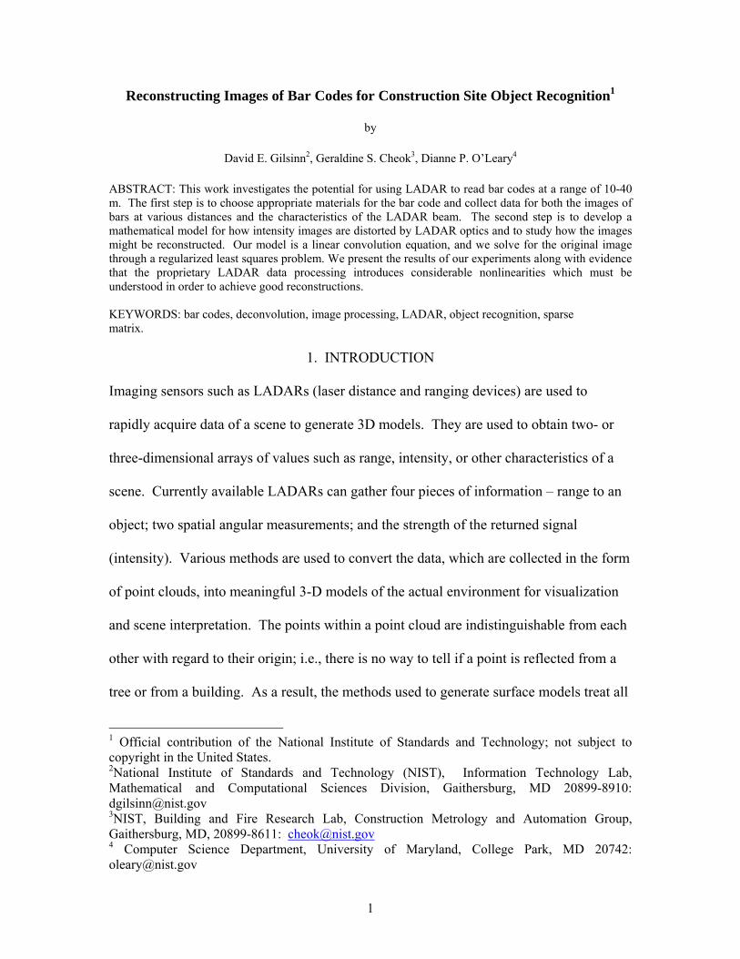
Reconstructing Images of Bar Codes for Construction Site Object Recognition1

by

David E. Gilsinn2, Geraldine S. Cheok3, Dianne P. O’Leary4

ABSTRACT: This work investigates the potential for using LADAR to read bar codes at a range of 10-40 m. The first step is to choose appropriate materials for the bar code and collect data for both the images of bars at various distances and the characteristics of the LADAR beam. The second step is to develop a mathematical model for how intensity images are distorted by LADAR optics and to study how the images might be reconstructed. Our model is a linear convolution equation, and we solve for the original image through a regularized least squares problem. We present the results of our experiments along with evidence that the proprietary LADAR data processing introduces considerable nonlinearities which must be understood in order to achieve good reconstructions. KEYWORDS: bar codes, deconvolution, image processing, LADAR, object recognition, sparse matrix.

1. INTRODUCTION

Imaging sensors such as LADARs (laser distance and ranging devices) are used to

rapidly acquire data of a scene to generate 3D models. They are used to obtain two- or

three-dimensional arrays of values such as range, intensity, or other characteristics of a

scene. Currently available LADARs can gather four pieces of information – range to an

object; two spatial angular measurements; and the strength of the returned signal

(intensity). Various methods are used to convert the data, which are collected in the form

of point clouds, into meaningful 3-D models of the actual environment for visualization

and scene interpretation. The points within a point cloud are indistinguishable from each

other with regard to their origin; i.e., there is no way to tell if a point is reflected from a

tree or from a building. As a result, the methods used to generate surface models treat all

1 Official contribution of the National Institute of Standards and Technology; not subject to copyright in the United States. 2National Institute of Standards and Technology (NIST), Information Technology Lab, Mathematical and Computational Sciences Division, Gaithersburg, MD 20899-8910: dgilsinn@nist.gov 3NIST, Building and Fire Research Lab, Construction Metrology and Automation Group, Gaithersburg, MD, 20899-8611: cheok@nist.gov4 Computer Science Department, University of Maryland, College Park, MD 20742: oleary@nist.gov

1

points identically and the results are indistinguishable “humps/bumps” in the scene

surface. Current surface generation methods, using LADAR data, require intensive

manual intervention to recognize, replace, and/or remove objects within a scene. As a

result, aids to object identification have been recognized by the end users as a highly

desirable feature and a high priority area of research.

The use of bar codes or UPC (Universal Product Code) symbols has become the universal

method for the rapid identification of objects ranging from produce to airplane parts. The

same method could also be used to identify objects within a construction scene. This

would involve using the LADAR to “read” a bar code. The concept is to use the intensity

data from the LADAR to distinguish the bar pattern. The advantage of this concept is

that no additional hardware or other sensor data is required to gather the additional data.

The basis for this concept lies in the high intensity values obtained from highly reflective

materials.

The challenges are the ability to read the bar code from 100 m or greater, distinguish bar

code points from the other points in the scene, capture a sufficient number of points to

define the bar code for correct identification, and the ability to read bar codes that are

skewed.

At ISARC 2001 [1] methods of determining the appropriate material for the bar codes

and determining if the use of bar codes was viable were reported. The results from these

efforts showed that at distances beyond 20 m (Figures 1 and 2), the intensity images were

too blurred to be readable and that image processing techniques were necessary to

2

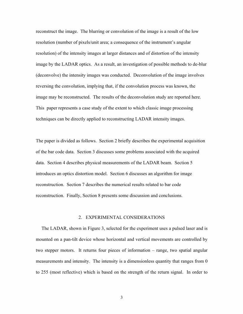
reconstruct the image. The blurring or convolution of the image is a result of the low

resolution (number of pixels/unit area; a consequence of the instrument’s angular

resolution) of the intensity images at larger distances and of distortion of the intensity

image by the LADAR optics. As a result, an investigation of possible methods to de-blur

(deconvolve) the intensity images was conducted. Deconvolution of the image involves

reversing the convolution, implying that, if the convolution process was known, the

image may be reconstructed. The results of the deconvolution study are reported here.

This paper represents a case study of the extent to which classic image processing

techniques can be directly applied to reconstructing LADAR intensity images.

The paper is divided as follows. Section 2 briefly describes the experimental acquisition

of the bar code data. Section 3 discusses some problems associated with the acquired

data. Section 4 describes physical measurements of the LADAR beam. Section 5

introduces an optics distortion model. Section 6 discusses an algorithm for image

reconstruction. Section 7 describes the numerical results related to bar code

reconstruction. Finally, Section 8 presents some discussion and conclusions.

2. EXPERIMENTAL CONSIDERATIONS

The LADAR, shown in Figure 3, selected for the experiment uses a pulsed laser and is

mounted on a pan-tilt device whose horizontal and vertical movements are controlled by

two stepper motors. It returns four pieces of information – range, two spatial angular

measurements and intensity. The intensity is a dimensionless quantity that ranges from 0

to 255 (most reflective) which is based on the strength of the return signal. In order to

3

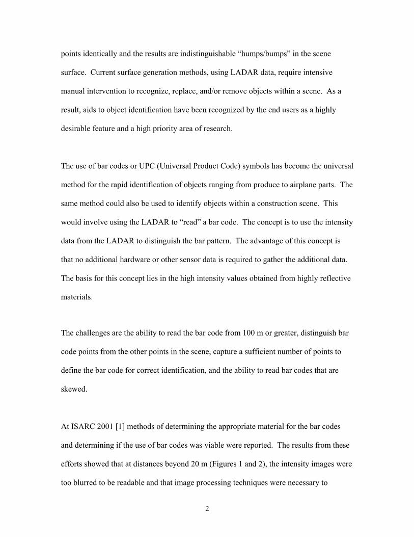
“read” the bar code, its existence has to be first established. To establish its existence,

the bar code has to have a unique feature or characteristic so that it is easily identifiable.

Therefore, the bar code would have to be made of a material that makes it easily

distinguishable from any background material based on the returned intensity value. A

good candidate material would be one that that would return an intensity that was both

much higher than any other material commonly found at a construction site and

Figure 1: Photograph of one set of the bar codes.

4

10 m 40 m20 m10 m 40 m20 m

Figure 2: LADAR images of the bar codes at three distances. Note the distorting of the image with distance.

that was consistently high for distances of 0 m to 150 m, i.e., intensity did not drop off

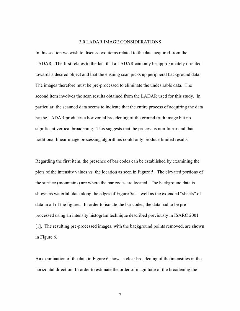
with distance. A reflective sheeting, that is a highly reflective prismatic lens sheeting

used for traffic signage, was used to construct the bar codes of Figure 1. This material

was chosen as it was readily available, durable, and would reflect light even if skewed

away from the light source. Sample photographs of the sheeting material are shown in

Figure 4. Figure 4 b shows that the sheeting is made of an array of prisms, each of which

has the capability of reflecting light in the direction from which it entered the prism.

5

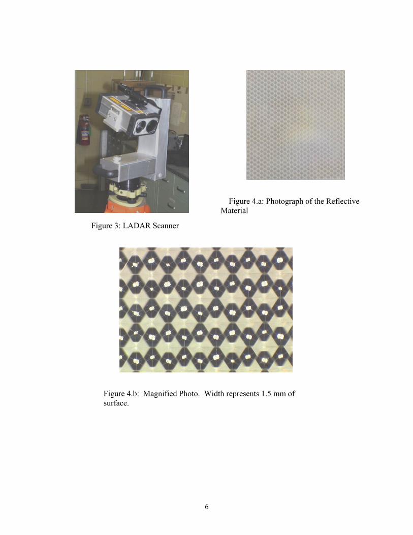
Figure 3: LADAR Scanner

Figure 4.b: Magnified Photo. Widsurface.

6

Figure 4.a: Photograph of the Reflective Material

th represents 1.5 mm of

3.0 LADAR IMAGE CONSIDERATIONS

In this section we wish to discuss two items related to the data acquired from the

LADAR. The first relates to the fact that a LADAR can only be approximately oriented

towards a desired object and that the ensuing scan picks up peripheral background data.

The images therefore must be pre-processed to eliminate the undesirable data. The

second item involves the scan results obtained from the LADAR used for this study. In

particular, the scanned data seems to indicate that the entire process of acquiring the data

by the LADAR produces a horizontal broadening of the ground truth image but no

significant vertical broadening. This suggests that the process is non-linear and that

traditional linear image processing algorithms could only produce limited results.

Regarding the first item, the presence of bar codes can be established by examining the

plots of the intensity values vs. the location as seen in Figure 5. The elevated portions of

the surface (mountains) are where the bar codes are located. The background data is

shown as waterfall data along the edges of Figure 5a as well as the extended “sheets” of

data in all of the figures. In order to isolate the bar codes, the data had to be pre-

processed using an intensity histogram technique described previously in ISARC 2001

[1]. The resulting pre-processed images, with the background points removed, are shown

in Figure 6.

An examination of the data in Figure 6 shows a clear broadening of the intensities in the

horizontal direction. In order to estimate the order of magnitude of the broadening the

7

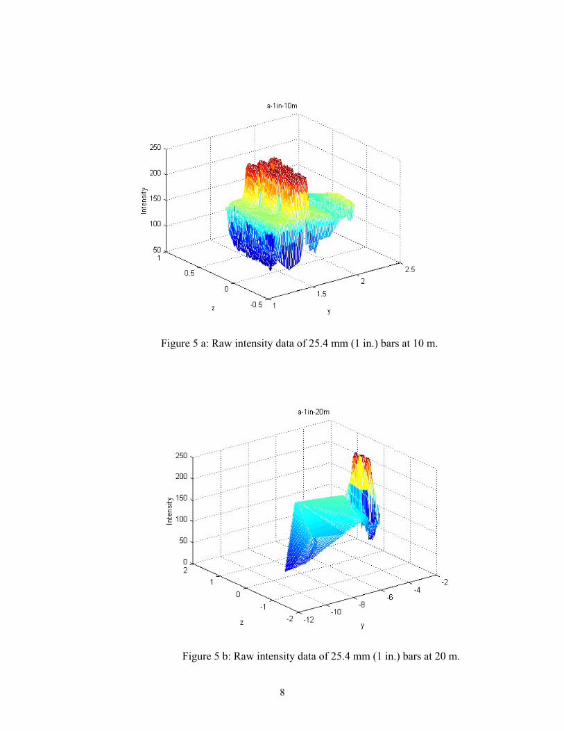
Figure 5 a: Raw intensity data of 25.4 mm (1 in.) bars at 10 m.

Figure 5 b: Raw intensity data of 25.4 mm (1 in.) bars at 20 m.

8

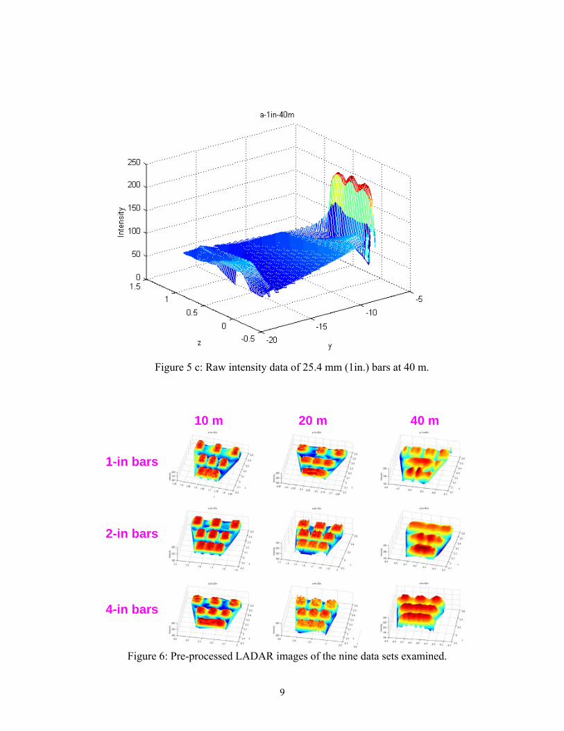
Figure 5 c: Raw intensity data of 25.4 mm (1in.) bars at 40 m.

10 m 20 m 40 m

1-in bars

2-in bars

4-in bars

Figure 6: Pre-processed LADAR images of the nine data sets examined.

9

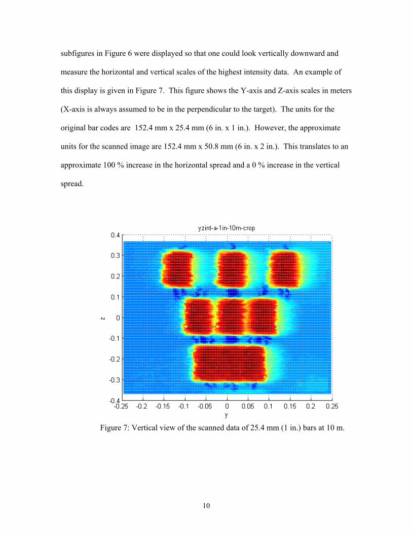
subfigures in Figure 6 were displayed so that one could look vertically downward and

measure the horizontal and vertical scales of the highest intensity data. An example of

this display is given in Figure 7. This figure shows the Y-axis and Z-axis scales in meters

(X-axis is always assumed to be in the perpendicular to the target). The units for the

original bar codes are 152.4 mm x 25.4 mm (6 in. x 1 in.). However, the approximate

units for the scanned image are 152.4 mm x 50.8 mm (6 in. x 2 in.). This translates to an

approximate 100 % increase in the horizontal spread and a 0 % increase in the vertical

spread.

Figure 7: Vertical view of the scanned data of 25.4 mm (1 in.) bars at 10 m.

10

4. BEAM SIZE AND DIVERGENCE ESTIMATION

In order to develop a model for image reconstruction it was necessary to understand the

divergence of the laser beam, i.e., how the laser beam changed as a function of distance.

The data for determining the beam size was obtained by measuring the dimensions of the

laser beam outline as projected on a white target. An infrared viewer was necessary to

see the projection of the laser on the target so that an outline of the beam could be drawn.

The outline of the beam was drawn by two or more observers and the measurements were

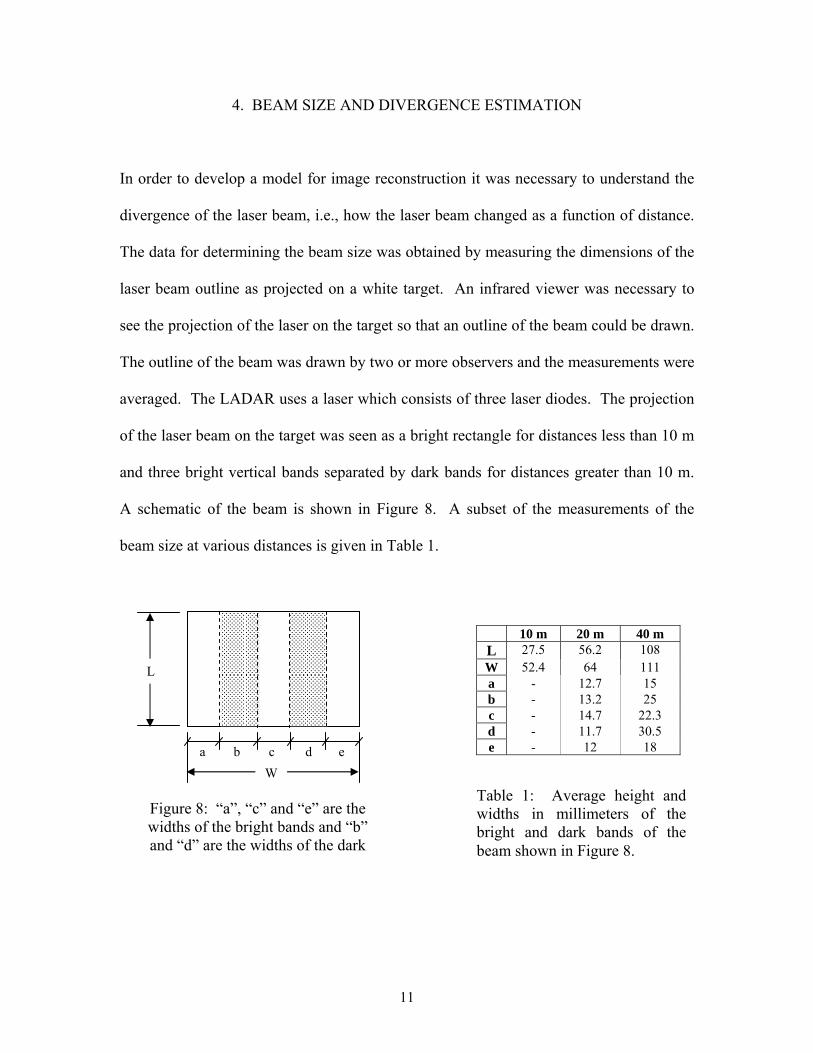
averaged. The LADAR uses a laser which consists of three laser diodes. The projection

of the laser beam on the target was seen as a bright rectangle for distances less than 10 m

and three bright vertical bands separated by dark bands for distances greater than 10 m.

A schematic of the beam is shown in Figure 8. A subset of the measurements of the

beam size at various distances is given in Table 1.

L

10 m 20 m 40 m L 27.5 56.2 108 W 52.4 64 111 a - 12.7 15 b - 13.2 25 c - 14.7 22.3 d - 11.7 30.5 e - 12 18

Table 1: Average height and widths in millimeters of the bright and dark bands of the beam shown in Figure 8.

d ea b c

W

Figure 8: “a”, “c” and “e” are the widths of the bright bands and “b” and “d” are the widths of the dark

11

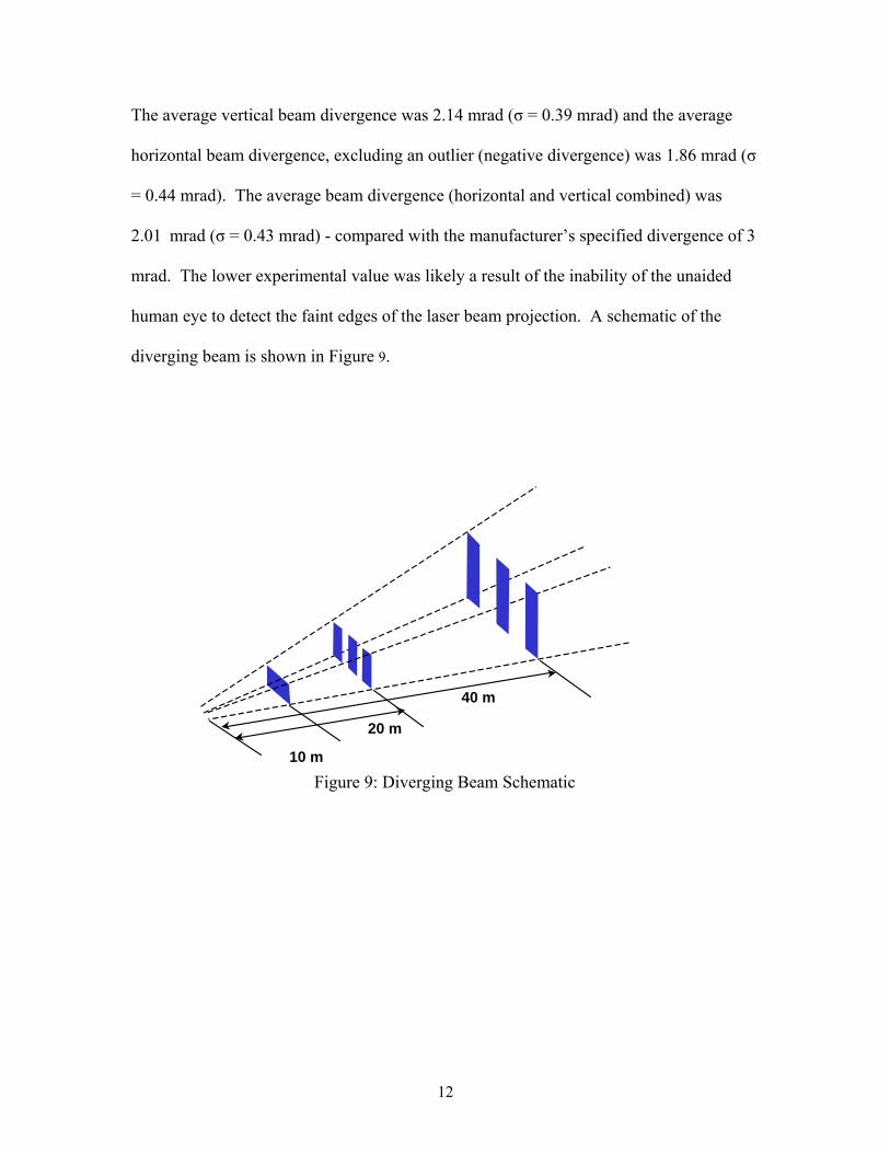
The average vertical beam divergence was 2.14 mrad (σ = 0.39 mrad) and the average

horizontal beam divergence, excluding an outlier (negative divergence) was 1.86 mrad (σ

= 0.44 mrad). The average beam divergence (horizontal and vertical combined) was

2.01 mrad (σ = 0.43 mrad) - compared with the manufacturer’s specified divergence of 3

mrad. The lower experimental value was likely a result of the inability of the unaided

human eye to detect the faint edges of the laser beam projection. A schematic of the

diverging beam is shown in Figure 9.

10 m

20 m

40 m

Figure 9: Diverging Beam Schematic

12

5. OPTICS MODEL FOR BEAM DISTORTION

For the purpose of developing an optics model of the distortion process involved with

LADAR imaging, we assume that there exists a data set representing bar codes on a 1 m

by 1 m board with intensity levels ranging from 0 to 255. This data set will be called the

ground truth. We will discretize the ground truth image by defining: 0 = y1 < y2 < … < ynf

= 1, 0 = z1 < z2 < … < znf = 1, y∆ i = yi+1- yi, = ∆ zj = zj+1- zj. = ∆ . The intensity at patch

y∆ i∆ zj is given by f(yi*, zj

*) y∆ i∆ zj where f is a function of (y, z) expressing the intensity

response at some point (yi*, zj

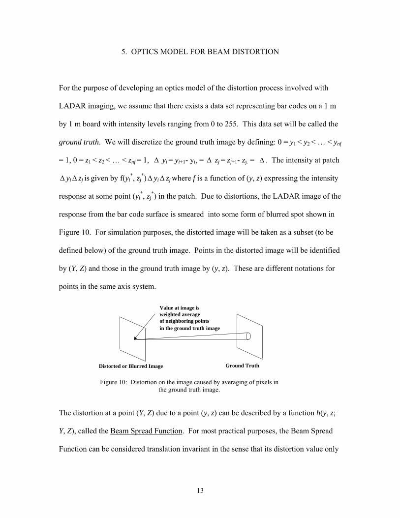
*) in the patch. Due to distortions, the LADAR image of the

response from the bar code surface is smeared into some form of blurred spot shown in

Figure 10. For simulation purposes, the distorted image will be taken as a subset (to be

defined below) of the ground truth image. Points in the distorted image will be identified

by (Y, Z) and those in the ground truth image by (y, z). These are different notations for

points in the same axis system.

The distort

Y, Z), calle

Function c

Ground TruthDistorted or Blurred Image

Value at image isweighted averageof neighboring pointsin the ground truth image

Figure 10: Distortion on the image caused by averaging of pixels inthe ground truth image.

ion at a point (Y, Z) due to a point (y, z) can be described by a function h(y, z;

d the Beam Spread Function. For most practical purposes, the Beam Spread

an be considered translation invariant in the sense that its distortion value only

13

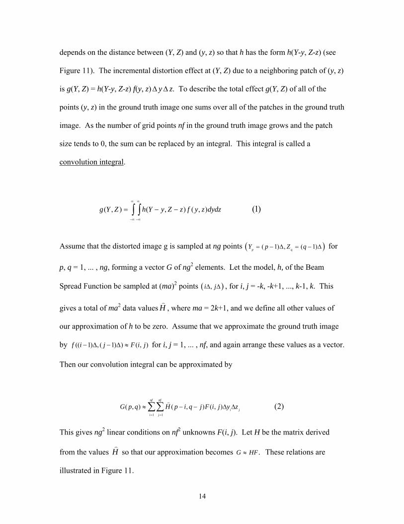
depends on the distance between (Y, Z) and (y, z) so that h has the form h(Y-y, Z-z) (see

Figure 11). The incremental distortion effect at (Y, Z) due to a neighboring patch of (y, z)

is g(Y, Z) = h(Y-y, Z-z) f(y, z) y∆ ∆ z. To describe the total effect g(Y, Z) of all of the

points (y, z) in the ground truth image one sums over all of the patches in the ground truth

image. As the number of grid points nf in the ground truth image grows and the patch

size tends to 0, the sum can be replaced by an integral. This integral is called a

convolution integral.

( , ) ( , ) ( , ) (1)∞ ∞

−∞ −∞

= − −∫ ∫g Y Z h Y y Z z f y z dydz

Assume that the distorted image g is sampled at ng points ( )( 1) , ( 1)p qY p Z q= − ∆ = − ∆ for

p, q = 1, ... , ng, forming a vector G of ng2 elements. Let the model, h, of the Beam

Spread Function be sampled at (ma)2 points ( ),i j∆ ∆ , for i, j = -k, -k+1, ..., k-1, k. This

gives a total of ma2 data values H , where ma = 2k+1, and we define all other values of

our approximation of h to be zero. Assume that we approximate the ground truth image

by (( 1) , ( 1) ) ( , )f i j F i− ∆ − ∆ ≈ j for i, j = 1, ... , nf, and again arrange these values as a vector.

Then our convolution integral can be approximated by

1 1

( , ) ( , ) ( , ) (2)= =

≈ − − ∆ ∆∑∑nf nf

i ji j

G p q H p i q j F i j y z

This gives ng2 linear conditions on nf2 unknowns F(i, j). Let H be the matrix derived

from the values H so that our approximation becomes .G HF≈ These relations are

illustrated in Figure 11.

14

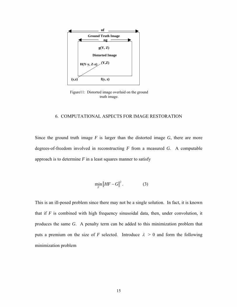
Ground Truth Image

Distorted Image

g(Y, Z)

(Y,Z)

(y,z) f(y, z)

H(Y-y, Z-z)

nf

ng

Figure11: Distorted image overlaid on the ground truth image.

6. COMPUTATIONAL ASPECTS FOR IMAGE RESTORATION

Since the ground truth image F is larger than the distorted image G, there are more

degrees-of-freedom involved in reconstructing F from a measured G. A computable

approach is to determine F in a least squares manner to satisfy

2min . (3)−F

HF G

This is an ill-posed problem since there may not be a single solution. In fact, it is known

that if F is combined with high frequency sinusoidal data, then, under convolution, it

produces the same G. A penalty term can be added to this minimization problem that

puts a premium on the size of F selected. Introduce λ > 0 and form the following

minimization problem

15

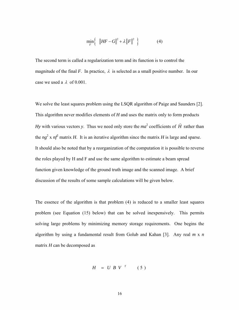
{ }2 2min (4)λ− +F

HF G F

The second term is called a regularization term and its function is to control the

magnitude of the final F. In practice, λ is selected as a small positive number. In our

case we used a λ of 0.001.

We solve the least squares problem using the LSQR algorithm of Paige and Saunders [2].

This algorithm never modifies elements of H and uses the matrix only to form products

Hy with various vectors y. Thus we need only store the ma2 coefficients of H rather than

the ng2 x nf2 matrix H. It is an iterative algorithm since the matrix H is large and sparse.

It should also be noted that by a reorganization of the computation it is possible to reverse

the roles played by H and F and use the same algorithm to estimate a beam spread

function given knowledge of the ground truth image and the scanned image. A brief

discussion of the results of some sample calculations will be given below.

The essence of the algorithm is that problem (4) is reduced to a smaller least squares

problem (see Equation (15) below) that can be solved inexpensively. This permits

solving large problems by minimizing memory storage requirements. One begins the

algorithm by using a fundamental result from Golub and Kahan [3]. Any real m x n

matrix H can be decomposed as

( 5 )= TH U B V

16

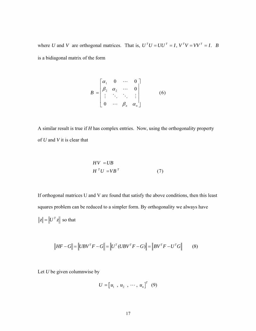
where U and V are orthogonal matrices. That is, B

is a bidiagonal matrix of the form

., IVVVVIUUUU TTTT ====

1

2 2

0 00

(6)

0 n n

B

αβ α

β α

⎡ ⎤⎢ ⎥⎢ ⎥=⎢ ⎥⎢ ⎥⎣ ⎦

A similar result is true if H has complex entries. Now, using the orthogonality property

of U and V it is clear that

(7)T T

HV UBH U VB

=

=

If orthogonal matrices U and V are found that satisfy the above conditions, then this least

squares problem can be reduced to a simpler form. By orthogonality we always have

zUz T= so that

( )T T T T THF G UBV F G U UBV F G BV F U G− = − = − = − (8)

Let U be given columnwise by

[ ]1 2, , , (9TnU u u u= )

17

where

1 (10)GuG

=

Then since U is orthogonal

11

21 1 1

10 0

(11)

0 0

T

TT

Tn

u Gu G

U G e

u G

β

β β

⎡ ⎤ ⎡ ⎤ ⎡ ⎤⎢ ⎥ ⎢ ⎥ ⎢ ⎥⎢ ⎥ ⎢ ⎥ ⎢ ⎥= = = =⎢ ⎥ ⎢ ⎥ ⎢ ⎥⎢ ⎥ ⎢ ⎥ ⎢ ⎥⎢ ⎥ ⎣ ⎦ ⎣ ⎦⎣ ⎦

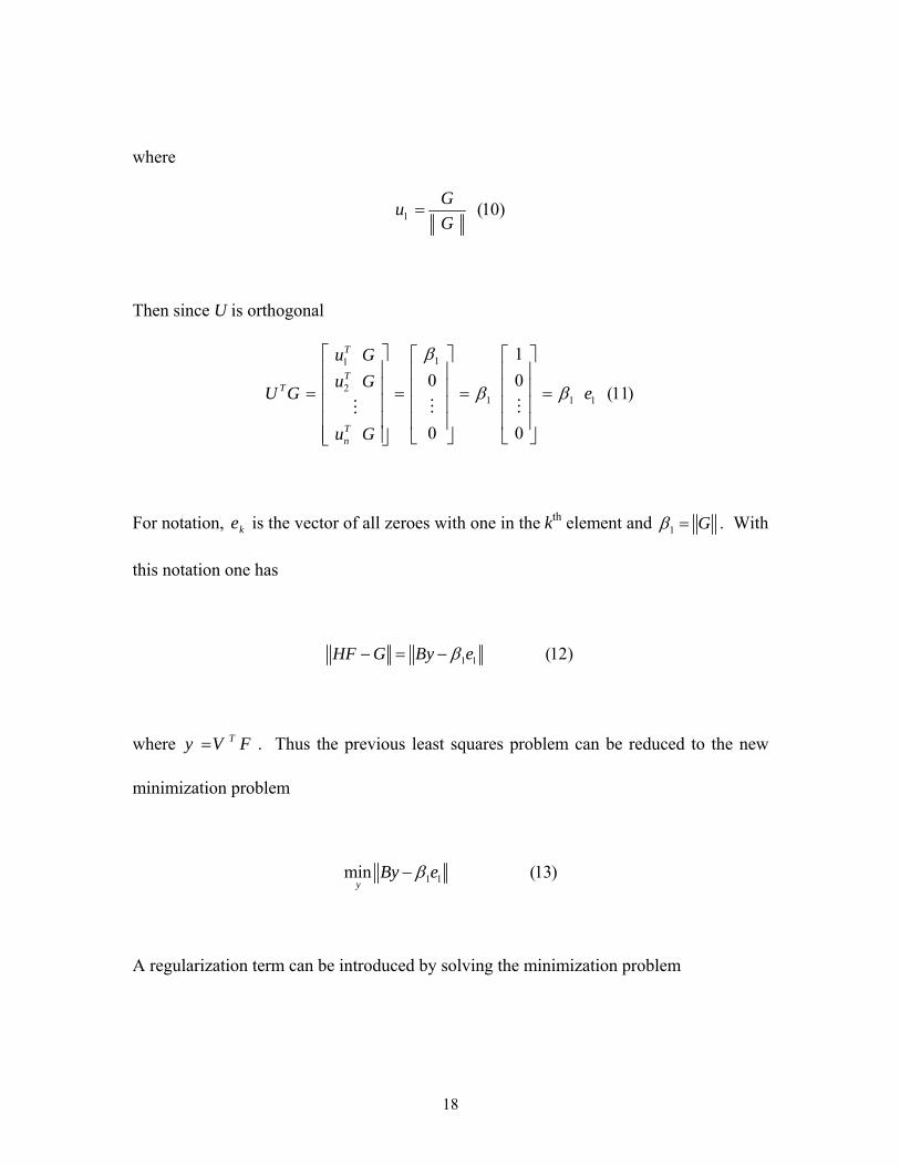
For notation, is the vector of all zeroes with one in the kke th element and 1β = G . With

this notation one has

1 1 (12)HF G By eβ− = −

where . Thus the previous least squares problem can be reduced to the new

minimization problem

Ty V F=

1 1min (13)y

By eβ−

A regularization term can be introduced by solving the minimization problem

18

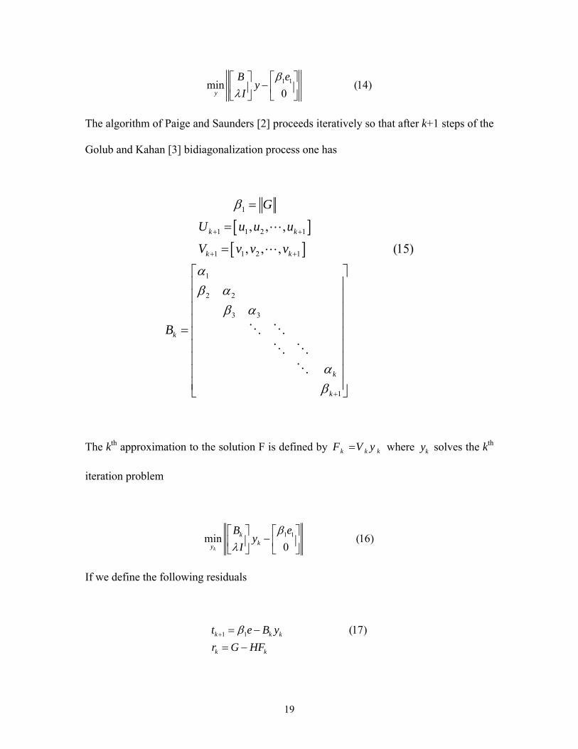
1 1min (14)0y

B ey

Iβ

λ⎡ ⎤ ⎡ ⎤

−⎢ ⎥ ⎢ ⎥⎣ ⎦ ⎣ ⎦

The algorithm of Paige and Saunders [2] proceeds iteratively so that after k+1 steps of the

Golub and Kahan [3] bidiagonalization process one has

[ ][ ]

1

1 1 2 1

1 1 2 1

1

2 2

3 3

1

, , ,

, , , (15)k k

k k

k

k

k

G

U u u u

V v v v

B

β

αβ α

β α

αβ

+ +

+ +

+

=

=

=

⎡ ⎤⎢ ⎥⎢ ⎥⎢ ⎥⎢ ⎥= ⎢ ⎥⎢ ⎥⎢ ⎥⎢ ⎥⎢ ⎥⎣ ⎦

The kth approximation to the solution F is defined by k kF V y k= where solves the kky th

iteration problem

1 1min (16)0k

kky

B ey

Iβ

λ⎡ ⎤ ⎡ ⎤

−⎢ ⎥ ⎢ ⎥⎣ ⎦ ⎣ ⎦

If we define the following residuals

1 1 (17)k k k

k k

t e B yr G HF

β+ = −= −

19

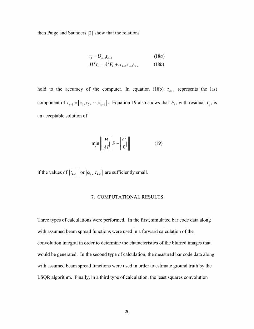
then Paige and Saunders [2] show that the relations

1 12

1 1 1

(18 )

(18 )k k k

Tk k k k k

r U t a

H r F vλ α τ+ +

+ + +

=

= + b

hold to the accuracy of the computer. In equation (18b) 1kτ + represents the last

component of [ ]1 1 2 1, , ,k kτ τ τ+ += kF krt . Equation 19 also shows that , with residual , is

an acceptable solution of

min (19)0x

H GF

Iλ⎡ ⎤ ⎡ ⎤

−⎢ ⎥ ⎢ ⎥⎣ ⎦ ⎣ ⎦

if the values of 1kt + or 1 1k kα τ+ + are sufficiently small.

7. COMPUTATIONAL RESULTS

Three types of calculations were performed. In the first, simulated bar code data along

with assumed beam spread functions were used in a forward calculation of the

convolution integral in order to determine the characteristics of the blurred images that

would be generated. In the second type of calculation, the measured bar code data along

with assumed beam spread functions were used in order to estimate ground truth by the

LSQR algorithm. Finally, in a third type of calculation, the least squares convolution

20

problem was re-written in such a fashion that the a beam function could be estimated

based on knowledge of the ground truth data and the measured bar code data.

In all of these calculations several classes of beam spread functions were used in the

numerical experiments. These included, for the 10 m data, a constant value over a

rectangular area, called an averaging filter. For the 20 m and 40 m data, beam spread

functions composed of three separate bars of constant values with zero assumed in

between the bars were used. These latter spread functions were developed in order to

simulate the splitting of the beam into three separate beams beyond 10 m. All of the

calculations, of course, had to be done for each of the three widths of the bar codes.

Measurements of spot data, used to simulate spike functions, were also used to construct

Beam Spread Functions (see Section 7.2 for more details on these functions).

7.1 Developing Simulated Bar Codes for Ground Truth

Determining ground truth for LADAR scans is not a well-defined process, which makes

it difficult to know whether a reconstruction is acceptable. For example, several issues

arise in comparing results to a photograph of the board on which the bar codes were

mounted. How far away from the camera should the board be placed in order to

construct the proper bar widths and heights? How can we minimize blurring caused by

the camera flash against the reflective material? How is a submatrix of greyscale pixels

extracted with reasonable ease from the dense digital image generated in a format such as

JPEG?

21

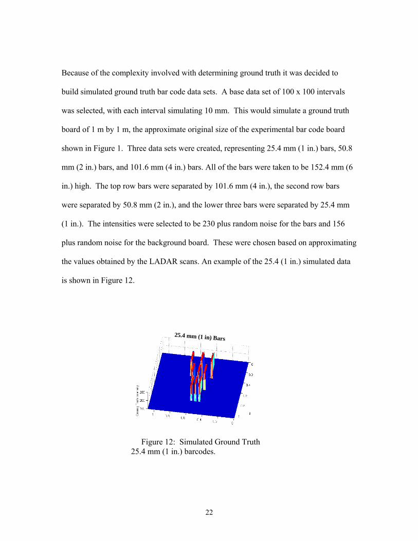
Because of the complexity involved with determining ground truth it was decided to

build simulated ground truth bar code data sets. A base data set of 100 x 100 intervals

was selected, with each interval simulating 10 mm. This would simulate a ground truth

board of 1 m by 1 m, the approximate original size of the experimental bar code board

shown in Figure 1. Three data sets were created, representing 25.4 mm (1 in.) bars, 50.8

mm (2 in.) bars, and 101.6 mm (4 in.) bars. All of the bars were taken to be 152.4 mm (6

in.) high. The top row bars were separated by 101.6 mm (4 in.), the second row bars

were separated by 50.8 mm (2 in.), and the lower three bars were separated by 25.4 mm

(1 in.). The intensities were selected to be 230 plus random noise for the bars and 156

plus random noise for the background board. These were chosen based on approximating

the values obtained by the LADAR scans. An example of the 25.4 (1 in.) simulated data

is shown in Figure 12.

Figure 12: Simulated Ground Truth 25.4 mm (1 in.) barcodes.

25.4 mm (1 in) Bars

22

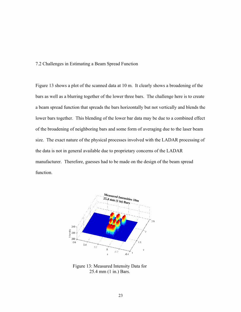
7.2 Challenges in Estimating a Beam Spread Function

Figure 13 shows a plot of the scanned data at 10 m. It clearly shows a broadening of the

bars as well as a blurring together of the lower three bars. The challenge here is to create

a beam spread function that spreads the bars horizontally but not vertically and blends the

lower bars together. This blending of the lower bar data may be due to a combined effect

of the broadening of neighboring bars and some form of averaging due to the laser beam

size. The exact nature of the physical processes involved with the LADAR processing of

the data is not in general available due to proprietary concerns of the LADAR

manufacturer. f the beam spread

function.

Therefore, guesses had to be made on the design o

Measured Intensities 10m 25.4 mm (1 in) Bars

Figure 13: Measured Intensity Data for

25.4 mm (1 in.) Bars.

23

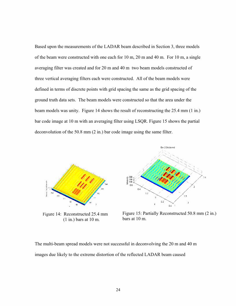
Based upon the measurements of the LADAR beam described in Section 3, three models of the beam were constructed with one each for 10 m, 20 m and 40 m. For 10 m, a single averaging filter was created and for 20 m and 40 m two beam models constructed of three vertical averaging filters each were constructed. All of the beam models were defined in terms of discrete points with grid spacing the same as the grid spacing of the ground truth data sets. The beam models were constructed so that the area under the beam models was unity. Figure 14 shows the bar code image at 10 m with an averaging filte deconvolution of the 50.8 mm (2 in.) bar code

Figure 14: Reconstructed 25.4 mm

(1 in.) bars at 10 m.

The multi-beam spread models were not succe

images due likely to the extreme distortion of

24

result of reconstructing the 25.4 mm (1 in.)

r using LSQR. Figure 15 shows the partial

image using the same filter.

Figure 15: Partially Reconstructed 50.8 mm (2 in.) bars at 10 m.

ssful in deconvolving the 20 m and 40 m

the reflected LADAR beam caused

potentially by beam interference or cross-talk, although this would have to be verified

through some form of calibration procedure.

Another class of beam spread function models was constructed. In classic optics, a point

spread function for a camera is usually developed by focusing the camera at a small

“point” of light in order to simulate as close as possible the effect of a light spike on the

camera. This is possible since the camera is a passive instrument in the sense that it

gathers light onto its backplane. The LADAR, however, is active in the sense that it

produces a beam that is scattered off of a target and then gathers the reflected light into

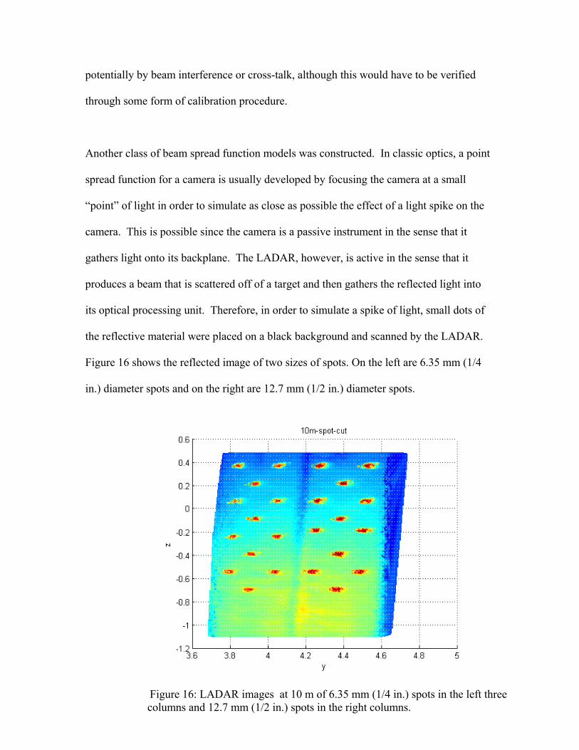
its optical processing unit. Therefore, in order to simulate a spike of light, small dots of

the reflective

Figure 16 sh

in.) diameter

material were placed on a black background and scanned by the LADAR.

ows the reflected image of two sizes of spots. On the left are 6.35 mm (1/4

spots and on the right are 12.7 mm (1/2 in.) diameter spots.

25

Figure 16: LADAR images at 10 m of 6.35 mm (1/4 in.) spots in the left three columns and 12.7 mm (1/2 in.) spots in the right columns.

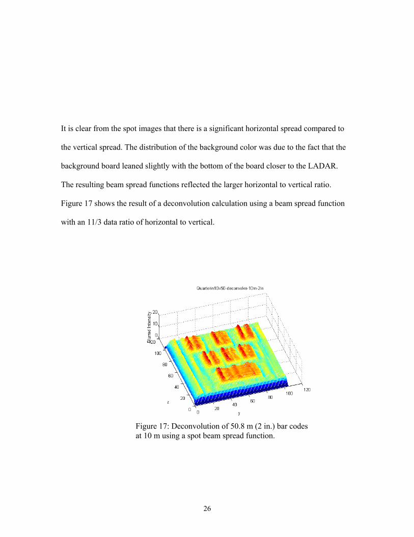
It is clear from the spot images that there is a significant horizontal spread compared to

the vertical spread. The distribution of the background color was due to the fact that the

background board leaned slightly with the bottom of the board closer to the LADAR.

The resulting beam spread functions reflected the larger horizontal to vertical ratio.

Figure 17 shows the result of a deconvolution calculation using a beam spread function

with an 11/3 data ratio of horizontal to vertical.

Figure 17: Deconvolution of 50.8 m (2 in.) bar codes at 10 m using a spot beam spread function.

26

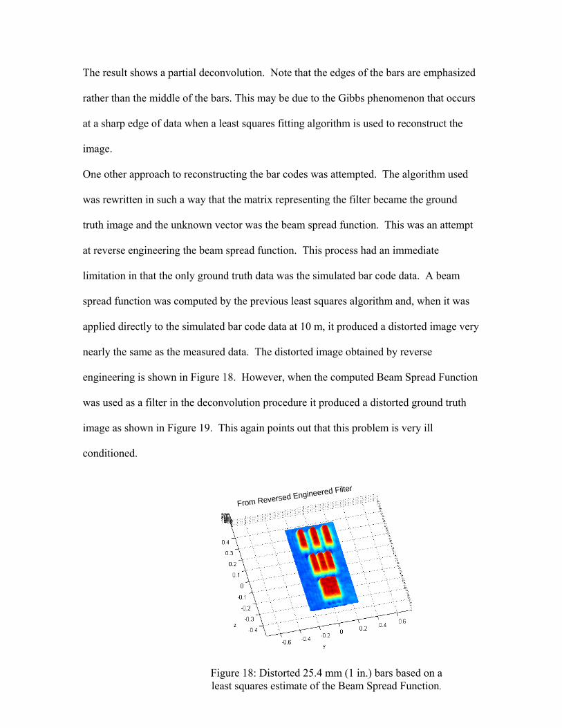
The result shows a partial deconvolution. Note that the edges of the bars are emphasized

rather than the middle of the bars. This may be due to the Gibbs phenomenon that occurs

at a sharp edge of data when a least squares fitting algorithm is used to reconstruct the

image.

One other approach to reconstructing the bar codes was attempted. The algorithm used

was rewritten in such a way that the matrix representing the filter became the ground

truth image and the unknown vector was the beam spread function. This was an attempt

at reverse engineering the beam spread function. This process had an immediate

limitation in that the only ground truth data was the simulated bar code data. A beam

spread function was computed by the previous least squares algorithm and, when it was

applied directly to the simulated bar code data at 10 m, it produced a distorted image very

nearly the same as the measured data. The distorted image obtained by reverse

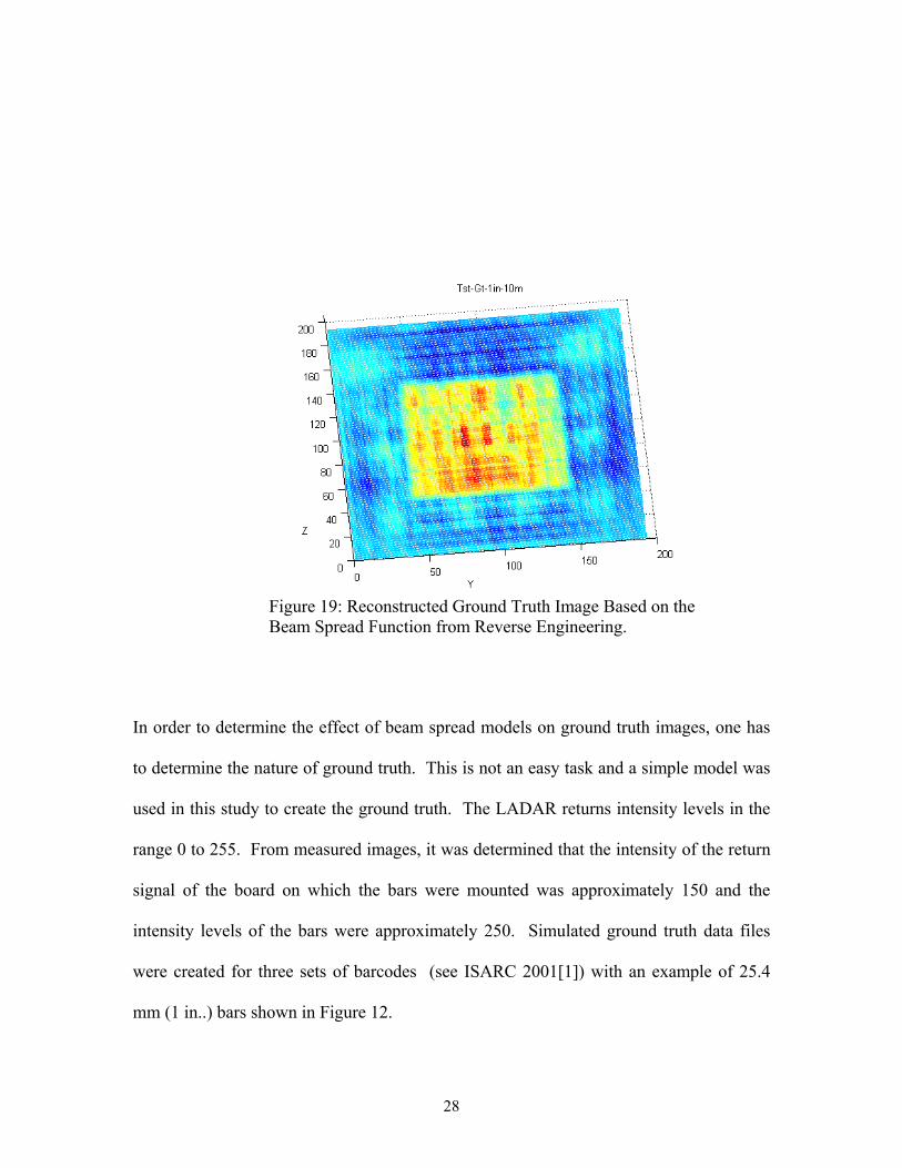
engineering is shown in Figure 18. However, when the computed Beam Spread Function

was used as a filter in the deconvolution procedure it produced a distorted ground truth

image as shown in Figure 19. This again points out that this problem is very ill

conditioned.

27

From Reversed Engineered Filter

Figure 18: Distorted 25.4 mm (1 in.) bars based on a least squares estimate of the Beam Spread Function.

In order to determ

to determine the n

used in this study

range 0 to 255. F

signal of the boa

intensity levels of

were created for t

mm (1 in..) bars sh

8. DISCUSSION AND CONCLUSIONS

Figure 19: Reconstructed Ground Truth Image Based on the Beam Spread Function from Reverse Engineering.

ine the effect of beam spread models on ground truth images, one has

ature of ground truth. This is not an easy task and a simple model was

to create the ground truth. The LADAR returns intensity levels in the

rom measured images, it was determined that the intensity of the return

rd on which the bars were mounted was approximately 150 and the

the bars were approximately 250. Simulated ground truth data files

hree sets of barcodes (see ISARC 2001[1]) with an example of 25.4

own in Figure 12.

28

Based upon the measurements of the beam spread function, three beam matrices were

created to represent the spread function at 10 m, 20 m, and 40 m. Since it was difficult to

obtain a precise measurement of the beam spread function, matrices representing the

three spatial beam spread configurations were created. They were defined in such a

manner that the area representing the dark regions was set to zero and the constant value

assigned to the light areas was chosen so that the volume under the bright bars summed to

unity. With the simulated barcodes and the simulated beam spread functions given,

convolution calculations were performed in order to determine how close the simulated

distorted images compared to the measured images. The simulated distorted images did

not reproduce the horizontal spread distortion observed in the measured images.

Although both the ground truth and beam spread images were simulated, it is likely that

the lack of prediction was caused mainly by poorly understood beam spread functions.

Since the preliminary measurements of the beam spread functions using an infrared scope

were crude, this is not surprising. Further study of the physical processes involved with

LADAR beams is needed.

As expected, the beam spread function changes at different distances. What was

surprising, though, was that a beam spread function could only partially reconstruct

different bar codes at the same distance. Thus, the beam spread function computed at 10

m for a given bar code size could not be used to deconvolve the image of the same bar

code size obtained at 20 m, but also could not be used to fully reconstruct 50.8 mm (2 in.)

bar codes at 10 m. The simulated beam spread function for 10 m was used to recover the

29

ground truth image, and the result is shown in Figure 14. An attempt was then made to

reconstruct the ground truth image for the 50.8 mm (2 in.) bars at 10 m with the same

simulated beam spread function. Figure 15 shows that the full reconstruction was not

completely obtained. This suggests that the beam spread function might be influenced by

the individual image being deconvolved, especially in the presence of noise. It, therefore,

is clear that the nature of the beam spread function and its relation to the image being

deconvolved is significant.

An attempt was then made to construct the beam spread function using the least squares

algorithm by setting the matrix H to be the ground truth image and the unknown F to be

the unknown beam spread matrix. Figure 18 shows the distorted image created for 25.4

mm (1 in.) bars using the best fit Beam Spread matrix. It is very close to the actual data

measured for the same bars as given in Figure 13. However, when used for

reconstruction it clearly fails as shown in Figure 19. All of the results, though, point to

the fact that reconstructing ground truth from distorted LADAR images is critically

dependent on knowledge of the Beam Spread Function and how it relates to individual

images.

The partial success obtained from the reconstruction of some bar codes at a distance of 10

m indicates that object identification from LADAR scans is potentially viable. However,

to be successful the object identification procedures appear to require some fundamental

physical knowledge that is lacking, such as the nature of LADAR beams, the divergence

of the beam, and the scattering characteristics of the scanned target. The internal

30

processing of the returned signal is another unknown since the information may not be

available for proprietary reasons. Coarse beam resolution also makes distinguishing fine

image elements difficult, if not impossible. This implies that the bar code size and

spacing play crucial roles in image reconstruction.

9. REFERENCES

1. W. C. Stone, G. S. Cheok, K. M. Furlani, D. E. Gilsinn, “Object Identification Using

Bar Codes Based on LADAR Intensity”, Proc. of the 18th IAARC / CIB / IEEE / IFAC

International Symposium on Automation and Robotics in Construction, ISARC 2001,

10-12 September, 2001, Krakow, Poland.

2. C. C. Paige, M. A. Saunders, ‘Algorithm 583: LSQR: Sparse Linear Equations and

Least Squares Problems’. ACM-Trans. Math. Software, Vol. 8, No. 2, Jun. 1982, pp.

195-209

3. G. Golub, W. Kahan, ‘Calculating the singular values and pseudo-inverse of a

matrix’, J. SIAM Numer. Anal., Ser. B, Vol. 2, No. 2, 1965, pp. 205-224.

31