Forschungsinstitut zur Zukunft der ArbeitInstitute for the Study of Labor

DI

SC

US

SI

ON

P

AP

ER

S

ER

IE

S

Recovery from Work and the Productivity ofWorking Hours

IZA DP No. 10103

July 2016

John Pencavel

Recovery from Work and the

Productivity of Working Hours

John Pencavel Stanford University

and IZA

Discussion Paper No. 10103 July 2016

IZA

P.O. Box 7240 53072 Bonn

Germany

Phone: +49-228-3894-0 Fax: +49-228-3894-180

E-mail: iza@iza.org

Any opinions expressed here are those of the author(s) and not those of IZA. Research published in this series may include views on policy, but the institute itself takes no institutional policy positions. The IZA research network is committed to the IZA Guiding Principles of Research Integrity. The Institute for the Study of Labor (IZA) in Bonn is a local and virtual international research center and a place of communication between science, politics and business. IZA is an independent nonprofit organization supported by Deutsche Post Foundation. The center is associated with the University of Bonn and offers a stimulating research environment through its international network, workshops and conferences, data service, project support, research visits and doctoral program. IZA engages in (i) original and internationally competitive research in all fields of labor economics, (ii) development of policy concepts, and (iii) dissemination of research results and concepts to the interested public. IZA Discussion Papers often represent preliminary work and are circulated to encourage discussion. Citation of such a paper should account for its provisional character. A revised version may be available directly from the author.

IZA Discussion Paper No. 10103 July 2016

ABSTRACT

Recovery from Work and the Productivity of Working Hours Observations on munition workers are organized to examine the relationship between their output each week, their working hours and days each week, and their working hours and days in adjacent weeks. The hypothesis is that workers need to recover from work and a long working week results in greater fatigue and stress and yet provides insufficient time for recuperation before the next week’s work opens. Workers require time off the job to restore their physical, mental, and emotional capacities and, if a long working week provides inadequate time to repair, their subsequent work performance suffers. JEL Classification: J24, J22, N34 Keywords: working hours, output, productivity, recovery Corresponding author: John Pencavel Department of Economics Stanford University Stanford, CA 94305-6072 USA E-mail: pencavel@stanford.edu

RECOVERY FROM WORK AND THE PRODUCTIVITY OF WORKING HOURS

John Pencavel*

Long hours and days of work injure workers’ health and impair individuals’ productivity at

their place of work.1 For instance, in one case, weeks during which workers were required to work

all seven days yielded about ten per cent less output than weeks in which the same number of hours

were allocated over six days; in short, seven days labor produces only six days’ output.2 The

hypothesis examined in this paper is that a long working week increases the need for workers to

recover from fatigue and stress, but a long working week may not leave enough restorative and

regenerative time for full recuperation for the following week’s work. The empirical research

reported below investigates whether a work schedule of continuous long working weeks has

measurable consequences for workers’ output.

Occupational health psychologists have presented evidence attesting to workers’ need to

recover from work and they have examined factors that frustrate and that expedite that recovery.

A necessary element of recovery is time not at work, time at the end of the working day and at the

end of the working week. Non-work time is essential but not sufficient for recovery because what

* I acknowledge with thanks helpful comments on an earlier draft from Jed DeVaro, Frank Wolak,

and two anonymous referees. I received excellent research assistance from Katy Bergstrom and

Monica Bhole.

1 On hours and health, among many studies, see Hulst (2003) and Conway et al.(2016). On hours

and worker productivity, see the references in Golden (2012).

2 See Pencavel (2015). The adage is cited in the Health of Munition Workers Committee (1919,

page 44 of Section VII).

2

appears to matter is how that non-work time is spent.3 By building on a previous investigation into

the productivity of working hours (Pencavel (2015)), this paper determines whether insufficient time

for workers to recover from a schedule of long working weeks impairs their performance at work.

Whereas much of the research in psychology relies upon self-reported well-being and psychological

feelings, the research here makes use of well-defined measures of time at work and the output of

piece-rate workers.

The setting for the empirical work that follows is the production of munitions in Britain

during the First World War, the Great War. The military’s demand for munitions was almost

insatiable and claims had circulated of a shell shortage, that the military lacked the matériel to fight

effectively. Men had volunteered in large numbers for the armed forces and their places in the

factories were taken by women, older men, and youths. Accompanying appeals that “A munition

worker is as important as the soldier in the trenches and on her his life depends”, women entered the

munition factories to such an extent that, by the end of the War, the majority of workers in munitions

production in Britain were women.

To produce the armaments demanded by the military, the working week was extended and

many regulations on employment set aside for the War’s duration. The long working weeks and

reports of unhealthy and unsafe conditions of production induced the government to set up an

3 A survey of over 12,000 workers employed in 45 companies in the Netherlands reported “some

degree of need for recovery from work....in nearly all employees” (Jansen, Kant, and Brandt (2002,

p. 322)). Time with family and friends and time devoted to physical activity appear to provide

effective renewal while time lost to poor sleep hinders restoration. These findings appear in Fritz

et al. (2010), Jacobsen et al.(2014), and Sonnentag and Zijlstra (2006), among others.

3

advisory group, the Health of Munition Workers Committee (HMWC), to recommend ways to

enhance the well-being and efficiency of munition workers.

The work undertaken on behalf of the HMWC included investigations by Dr. Horace M.

Vernon, M.D., Fellow of Magdalen College, Oxford into the weekly hours and days of work and the

weekly output of various groups of workers at a Midlands munitions factory from November 1915

to December 1916. Information on piece-rate workers’ output was gathered from payroll records;

the workers were unaware their work performance was being analysed. The HMWC’s inferences

and recommendations rested, in part, on Vernon’s data and a subset of these observations forms the

basis of the empirical work below.

I. OBSERVATIONS USED IN THIS ANALYSIS

Hours of Work

The observations on hours of work are not those set by the employer nor those reported by

the employees, but those observed and calculated by Vernon, the investigator. From watt-meters that

recorded the electric power supplied to various work stations, Vernon gauged “broken time” as the

sum of the minutes taken before starting work in the morning and after lunch, the minutes used in

stopping work before lunch and before finishing at the end of the day, and the minutes over the day

when work slackened.4 Any changes in the length of work breaks are reflected in broken time.

To “broken time” was added time due to absences and time of those putting in “short weeks”

4 Vernon writes, “The machinery is started running shortly before work begins, and as the operatives

get going, one after another, the power consumption steadily rises to a maximum, which is attained

when all operatives have started. By means of these power records the rate of starting and stopping

work can easily be ascertained” (¶ 29 of HMWC 1916).

4

to arrive at total “lost time”. This was subtracted from scheduled hours (or what Vernon called

“nominal” hours) to determine actual hours at work. These calculations were conducted for each

week and for each group of workers. Clearly, Vernon went to uncommon lengths to take account

of time not worked. The association between output and hours measured in this paper uses actual

hours worked, not scheduled hours, although the correspondence between movements in scheduled

weekly hours and in actual weekly hours is high: relative variations in scheduled hours map one-for-

one into relative variations in actual hours worked.5

Other Inputs in Production

During the period of observation from the autumn of 1915 to the end of 1916, Vernon states

that “....there were no changes whatever in the conditions of production of the articles, such as the

character of the machinery and its speed, and in the nature and quality of the articles produced”

(Vernon (1921, p. 38)). There were changes in hours and days worked: after eighteen months from

the opening of the war, there was a decline in weekly hours of work because of the realisation that

“long hours did not pay” (Vernon (1921, p.34)).

As for the skills of the workers, Vernon reports that, as “the great majority of munition

workers during the war” had not been employed in these activities before the war, to allow them

to gain experience, he did not use observations on the workers early in their tenure and he waited

until

5 If H j t denotes actual hours worked by workers belonging to group j in week t and if (H j t )SC is

scheduled hours, then the least-squares regression of the logarithm of actual hours on the logarithm

of scheduled hours for the 102 observations used below yields the following estimates:

log[ H j t ] = -0.180 + 1.013 log[( Hj t )SC ] , R 2 = 0.944 .

5

they had reached their full and steady output.6 There was a little turnover “....although the majority

of the workers at the beginning were present at the end” (Vernon (1921, p.21)). Consequently,

physical capital and workers’ skills are taken as fixed over the weeks that constitute the observation

period.

Interpretation

When relating the average weekly output of a group of workers to their time worked, whose

behavior is being described - the behavior of the workers or that of the employer? In the absence

of a body such as a trade union and within the limits set by any enforced statutory regulation, the

employer sets the work schedule, the starting and ending times, and the days worked. These

scheduled hours are in response to the demand for the factory’s product and reflect the employer’s

understanding of the hours required of employees to yield the desired output.7 Weekly variations

6 “Since most of their work was of a comparatively simple repetition character, they soon attained

a steady output....my method was to study the output of a group of experienced women for several

months, and at the end of that time to replenish the reduced numbers [through turnover] by the

addition of comparatively fresh workers....It was found that the fresh workers (provided they had

had one month’s experience) achieved as great an output as experienced workers of five months’

service so the introduction of the fresh blood did not appreciably alter output” (Vernon (1921,

p.39)).

7 Before the war, at a time when working hours were often greater than ten hours a day for six or

more days each week, many employers opposed proposals to reduce working hours. Hicks (1932,

p. 107 ) doubted that the typical employer understood the relationship between working hours and

employees’ output. Also see Nyland (1989).

6

in scheduled hours of work arose from the military’s preparations for major offensives such as the

Battle of the Somme.8 They also arose from customary shorter weeks at times such as Christmas

and Easter. Two weeks record shorter hours because of a temporary shortage of material.

Vernon states there were no group restrictions on output in which case the individual worker

determines her effort each hour in a given week and this will change with variations in the

(pecuniary and non-pecuniary) returns to effort and with variations in her energy and disposition.

The workers were paid on piece-rates but Vernon does not report any movements or differences in

these rates beyond the statement that they were high enough to enable the worker to enjoy higher

take-home pay than before the war. In short, it seems reasonable to take variations in hours worked

as set by the employer whereas variations in effort and, consequently, in output are chosen by

workers according to their capacities and proclivities.

Selecting the Observations

The goal of this analysis is to determine whether work performance is associated not only

with current input levels but also with inputs in other periods. Vernon’s data offer an opportunity

to address this because most of his weekly observations relate to adjacent weeks: of the 122 weekly

observations analysed previously (Pencavel (2015)) on hours and output for four groups of workers,

106 of these observations relate to contiguous weeks for three of the four groups of workers; that

is, for 87 per cent of the 122 weeks, we know not only how many hours and days were worked in

a week but also how many hours and days were worked in the preceding week. Thus, sixteen

observations will be omitted from the set of 122 weekly observations for lack of information about

8 For the bombardment of enemy lines preceding the British infantry’s advance on 1 July 1916,

“.....nearly three million shells” were stockpiled (Keegan (1999), p. 291).

7

the previous week’s work.

Four observations record the previous week’s working hours and days to be zero: these

weeks were holidays. At first sight, the presence of holidays would seem to provide an excellent

opportunity to consider the restorative effects of fewer hours and days of work. Indeed,

contemporary research has investigated the effects of holidays on subsequent work performance.9

However, in this case, four observations provide very little information to examine this connection

and, although an effort was made to measure an association between a holiday one week and output

the following week, little of economic and statistical significance came from these efforts. Because

retaining these four observations would require methods for dealing with distinct outliers,10 a simpler

and less contentious procedure is simply to drop these four observations from the estimating sample.

Hence from the earlier set of 122 weekly observations, 16 observations were dropped by

necessity because of the absence of information on the previous week’s working hours and days and

another 4 observations were dropped because the previous week was not a working week. The

remaining 102 observations constitute the basic sample to which estimating equations were fitted.

Descriptive statistics on the 102 weekly observations are given in the upper panel of Table 1 where

X j t denotes the average weekly output of group j workers in the week ending t , H j t stands for the

hours worked by group j workers in week ending t , and S j t is a dichotomous variable that takes the

value of unity when group j workers worked on a Sunday in week t and of zero otherwise. Sunday

9 For instance, see Fritz and Sonnentag (2006) and Westman and Etzion (2001).

10 The lowest (positive) value of a previous week’s working hours is 24 so zero working hours (in

the previous week because of a holiday) would constitute an evident outlier.

8

work is taken to mean that a seven day week was worked.11 Most of the seven day weeks were

worked in 1915 and in the first half of 1916. Weekly hours of work range from 24 hours to almost

72.12

There are three groups of workers contained in these 102 weekly observations: 53 of the

observations are on 100 women turning fuze bodies, 22 observations are on 40 women milling a

screw thread, and 27 observations are on 56 men sizing fuze bodies. Each group of workers has its

distinct output and the investigator converted this to an index number. Any differences in the base

value of the index will be absorbed in estimation in group fixed effects. These 102 observations will

be used to relate the average output of these workers in each week t to hours and days worked during

week t and also to hours and days worked in previous weeks.

11 A week around a holiday may have entailed Sunday work in lieu of work on another day though

Vernon (1921, p. 115) observes that “the weekly day of rest is almost always taken on Sunday”.

Naturally, hours of work tend to be longer in weeks involving seven work days: the average value

of H j t is 45.3 when S j t = 0 whereas the average value of H j t is 58.2 when S j t = 1 . In these data,

S j t is never a fraction between zero and unity which would occur if some members of a group

worked seven days and others worked fewer.

12 The unusual 24 hour week (for the women turning fuze bodies) arises because the government

called for four days of holiday in the week ending 30 September 1916 as compensation for the loss

of holidays over the summer. The women milling a screw thread worked 26.4 hours and the men

sizing fuze bodies worked 28.2 hours this week.

9

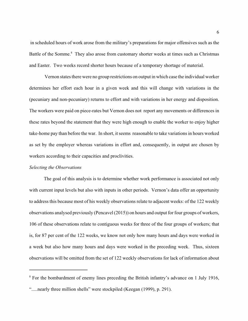
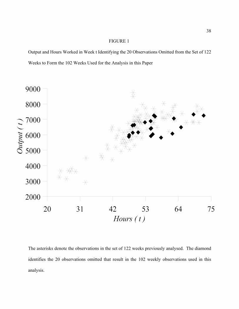
Figure 1 provides a visual impression of the relation between week t’s output and week t’s

hours with the twenty observations omitted from the earlier 122 observations identified by a

diamond; an asterisk distinguishes the remaining 102 observations. Clearly those observations

omitted from the set of 122 weeks tended to be those weeks where hours of work are long. In

moving from the set of 122 observations to the 102 observations that constitute the set to which the

equations in this paper are fitted, no observation corresponding to fewer than 46 working hours is

omitted. Sixteen of the twenty observations omitted from the set of 122 have values of weekly hours

greater than 49. The observations used in the work reported in this paper are more heavily weighted

towards shorter hours than the previous set. This may imply that aspects of the relationships fitted

in this paper will not replicate those reported in earlier work.

Notwithstanding the non-random loss of observations, is the relation between output and

labour established in previous research (Pencavel (2015)) that analysed 122 weeks also evident in

the 102 observations studied here? Previous research documented a nonlinear relationship between

weekly output and weekly hours of work: approximately, output rises with hours but the increase

in output falls as hours increase. In addition, a seven day working week reduces weekly output

holding hours constant. To assess whether this pattern is evident in the 102 weekly observations

analysed in this paper, the following production function is specified:

(1) X j t = α 0 + α 1 H j t + α 2 ( H j t ) 2 + η S j t + ω j + ε 1 j t

where the fixed number of workers, plant, equipment, and production speed are contained in the

equation’s intercept, group-specific fixed effects are represented by ω j and other influences on

10

output are gathered in an assumed well-behaved error term, ε 1 j t .

The least-squares estimates of equation (1) are in column (1a) of Table 2 from which it is

evident that, as in earlier research using 122 observations, output rises with hours but at a decreasing

rate signifying that, at all hours, the marginal product of hours falls as hours increase. One

difference from previous research is that equation (1a) implies that output reaches a maximum at

longer hours than those implied in the earlier research (holding days worked constant). The loss in

output from denying workers a day of rest is twelve per cent when evaluating the estimated

coefficient on S j t at the mean value of output. This estimate is close to that reported from using all

122 observations.

II. EFFECTS OF HOURS AND DAYS WORKED IN THE PREVIOUS WEEK

The research presented in this paper is directed toward determining whether a long working

week provides inadequate time for workers to restore their physical, mental, and emotional reserves

before the subsequent working week opens. If recovery from the week’s work is incomplete, the

workers’ performance in the subsequent week may suffer. This suggests that output in week t

depends not only on hours and days worked in week t , but also on the previous week’s working

hours and days, H j t - 1 and S j t - 1, respectively.

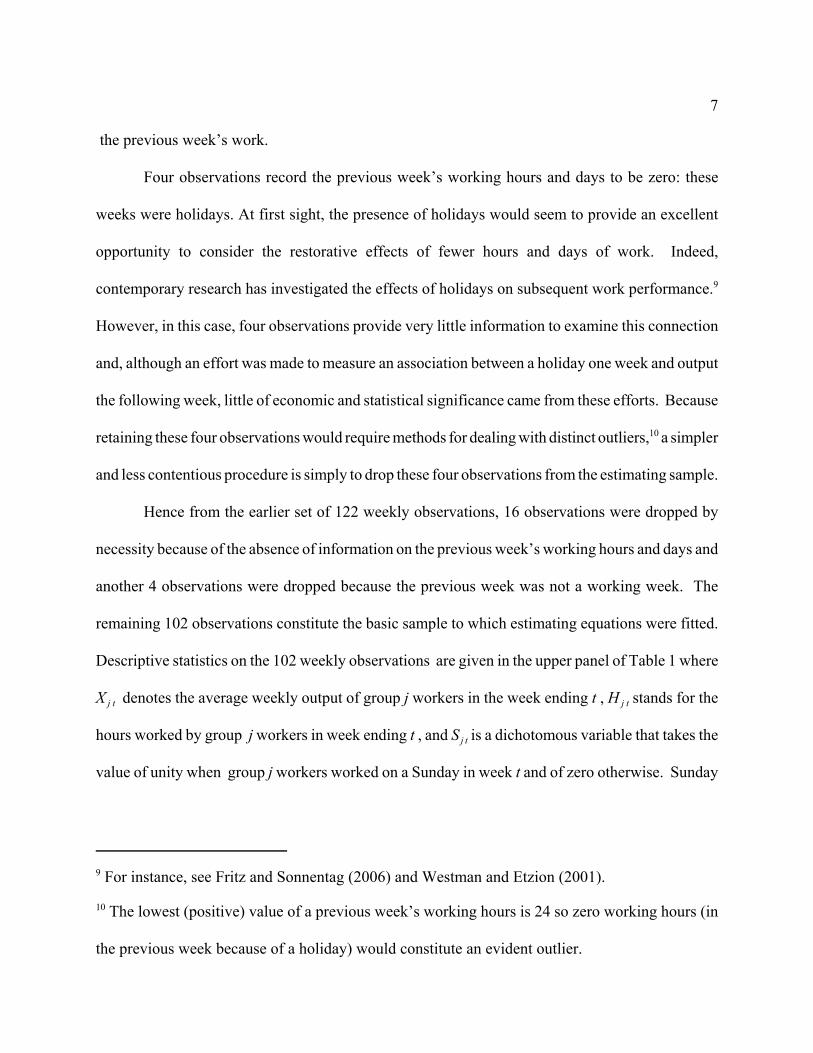
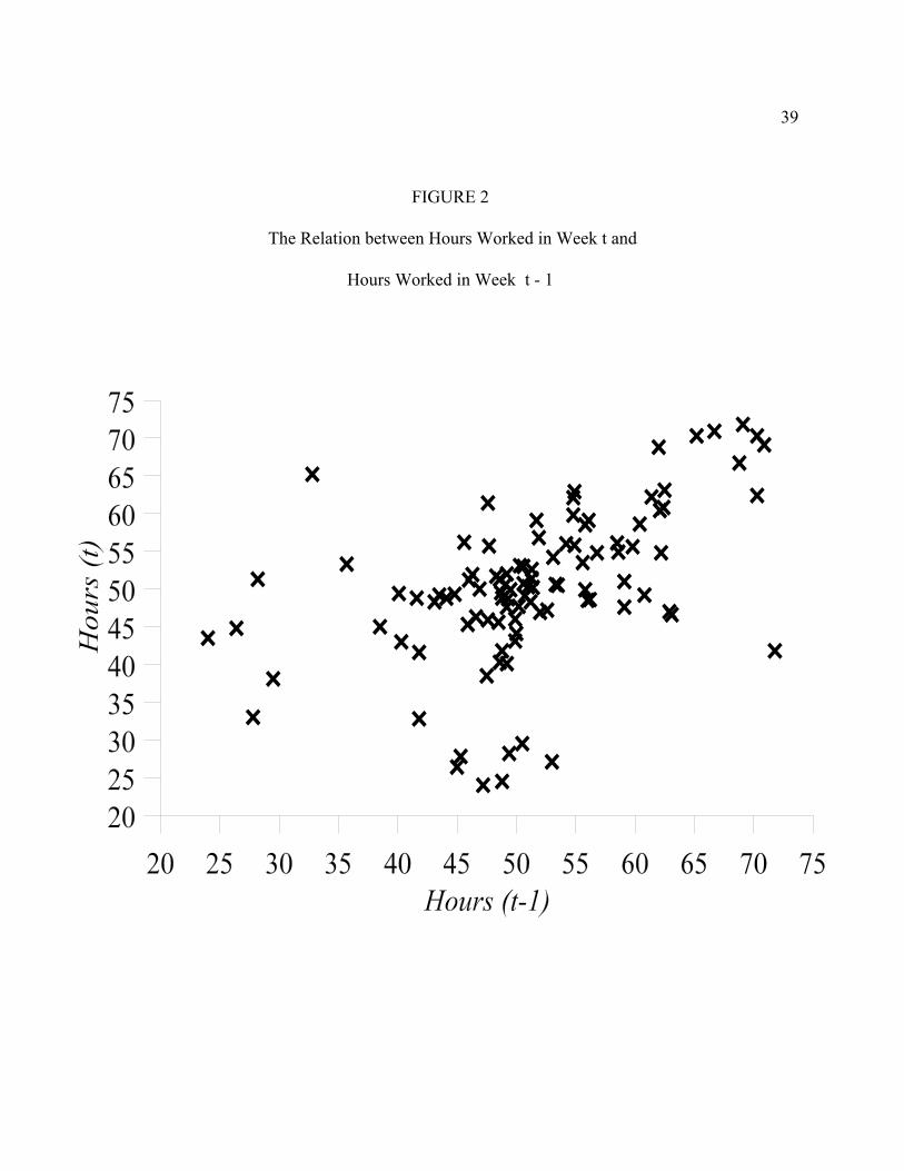
The correspondence between H j t and H j t - 1 is pictured in Figure 2 from which a positive

association is evident. The simple correlation coefficient between H j t and H j t - 1 for these 102

observations is + 0.504. Of the 50 weeks with H j t longer than 50 hours, 78 percent were preceded

by weeks also longer than 50 hours. The positive serial correlation in hours suggests a working

schedule that does not compensate for a long work week in one week with a shorter working week

11

in the following week. On the contrary, there is persistence in weekly hours of work, the

consequences of which are examined below.

The hypothesis that a long working week in week t-1 affects output in week t requires

determining the hours that constitute a long working week. The procedure is to specify a flexible

relationship between X j t and H j t-1 that permits the consequences of long working hours to be

revealed. To this effect, conditional upon the output-labour relationship in week t taking the form

of equation (1), write the weekly production function as a quadratic spline function in H j t-1 :

(2) X j t = α 0 + α 1 H j t + α 2 ( H j t ) 2 + η S j t + [ β 0 + β 1 (H j t - 1 - H o ) + β 2 ( H j t - 1 - H o )

2] K 1 j t - 1

+ [ β 3 + β 4 (H j t - 1 - H K ) + β 5 ( H j t - 1 - H K ) 2] K 2 j t - 1 + μ S j t - 1 + ω j + ε 2 j t .

In fitting equation (2) , the observations are sorted into two regimes based on hours worked in week

t - 1: the shorter hours regime consists of observations for which hours are less than the knot H K and

the longer hours regime consists of observations where hours are equal to or greater than H K. Within

each regime, the output-hours relation follows its own quadratic-in-hours pattern and they are

estimated under the constraint that the two expressions meet smoothly at the knot. This constraint

at the knot places restrictions on the coefficients in the two regimes. K 1 j t takes the value of unity

for observations on H j t - 1 in the shorter hours regime and of zero otherwise while K 2 j t is unity for

observations on H j t - 1 in the longer hours regime and is zero otherwise. ε 2 j t is a stochastic

disturbance embodying omitted factors. Group-specific fixed effects are again represented by ω j.

12

The effect on output in week t of a seven day working week in t - 1 holding H j t and H j t - 1 constant

is measured by μ . In all cases, the value of H o is set to 24 hours, the lowest value of hours observed

in these data. Equation (2) is estimated by least-squares setting different values for the knot H K

between 45 hours and 60 hours and the estimates in column (2a ) of Table 3 correspond to a knot

of 53 hours. Higher and lower values of the knot did not improve explanatory power although there

are small differences in the fitted equation when other knots are specified. There are 39 weekly

observations in the longer hours regime and 63 observations in the shorter hours regime. The

estimates in column (2a ) correspond to an equation in which lagged hours of work take a quadratic

form in both the shorter and the longer hours regime, but those corresponding to the shorter hours

regime are imprecisely estimated. This prompts the question of whether the shorter hours regime

may be characterised more parsimoniously than the quadratic specified.

In particular, consider the hypothesis that, holding hours and days worked in week t constant,

output in week t is independent of hours worked in week t - 1 provided hours in week t - 1 are less

than or equal to the knot of 53 hours whereas output in week t is responsive to hours longer than 53

in week t - 1. In terms of equation (2), the parameters β 1 and β 2 are constrained to zero and the

relation in the longer hours regime remains a quadratic in H j t-1 . If the spline continues to require

that the relation in the shorter hours regime meets the relation in the longer hours regime smoothly,

then when β 1 and β 2 are zero, so is β 4 and equation (2) takes the contracted form of

(3) X j t = α 0 + α 1 H j t + α 2 ( H j t ) 2 + η S j t + β 5 ( H j t - 1 - H K ) 2 K 2 j t - 1 + μ S j t - 1 + ω j + ε 3 j t .

13

Can this restricted form of equation (2) be rejected by these observations? The answer is “no”: the

estimates of equation (3) when fitted to the 102 observations are reported in column (3a ) of Table

3 where the goodness of fit statistics indicate the estimates of equation (3) involve virtually no loss

in explanatory power notwithstanding fewer right-hand side variables. A formal F test is consistent

with this.

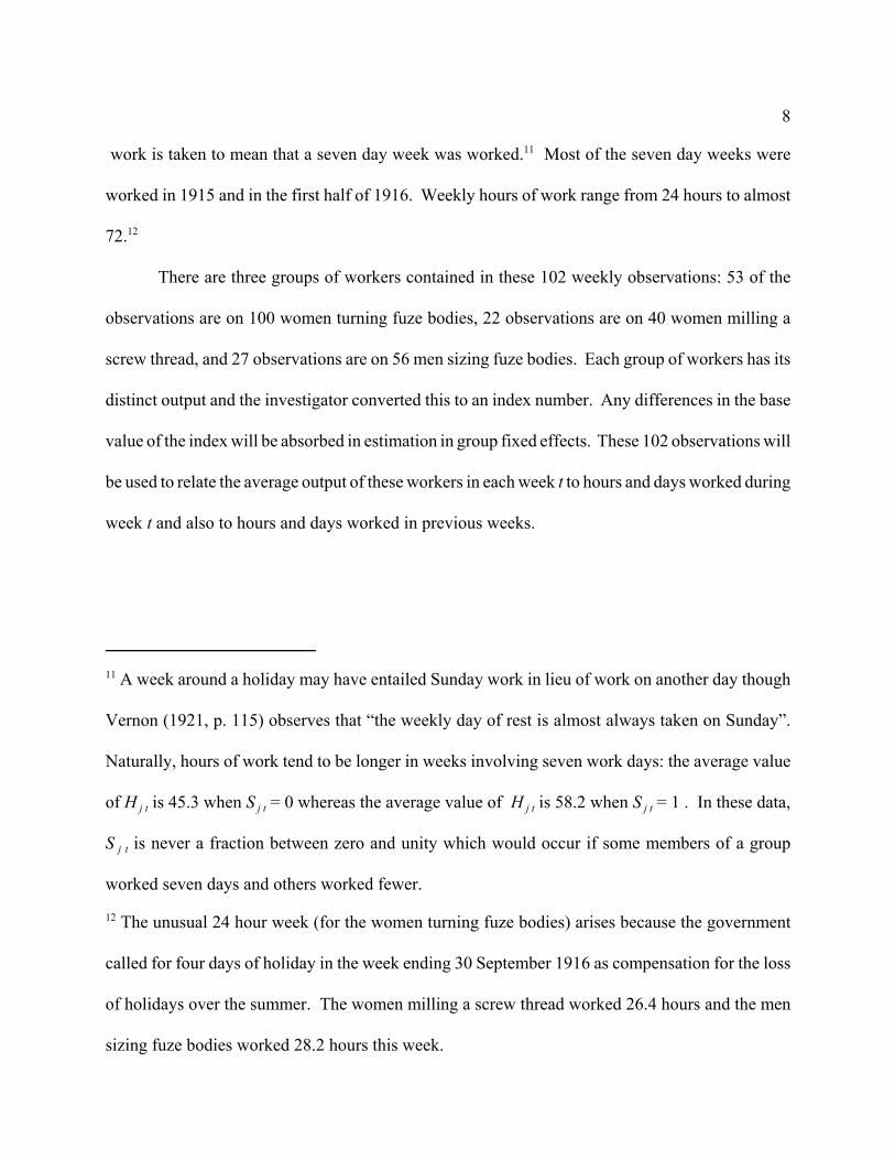
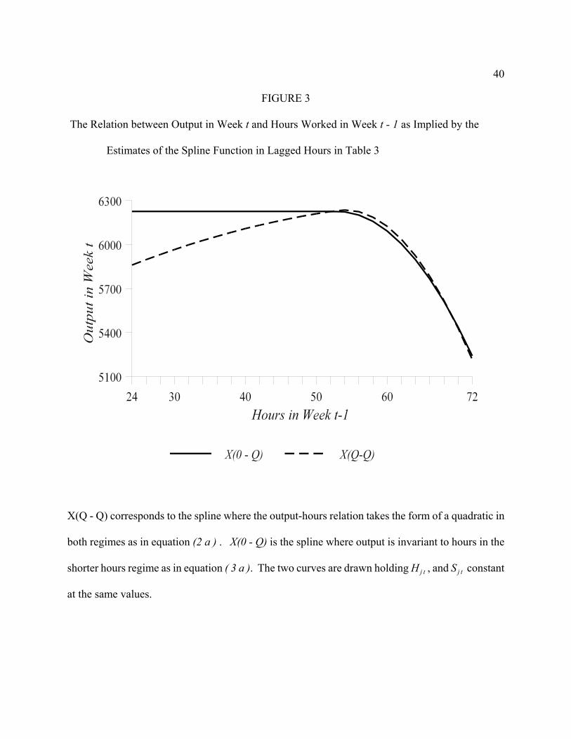
A visual comparison of the relation between X j t and H j t -1 implied by the estimates in

columns ( 2a ) and ( 3a ) of Table 3 is provided in Figure 3: the relation between X j t and H j t -1

implied by the estimates of equation (2 a) are given by the dashed curve X( Q - Q ) whereas those

implied by the estimates of equation (3 a) are given by the solid curve X(0 - Q) according to which

output in week t is independent of the previous week’s hours until H j t -1 reaches 53 hours after

which output declines unmistakably and monotonically.13 In short, only long hours worked in week

t - 1 damage output in week t .

The estimates of equation (3 a) imply that output in week t rises with hours worked in week

t, but the magnitude of the rise decreases as hours increase; output is predicted to reach a maximum

when H j t equals 99 hours, a value considerably above the highest value of hours observed in these

data. The hours of maximum output are also greater than those reported in Pencavel (2015) that

used 122 weekly observations.14

13 Given the specification of equations (2) and (3), of course, the shape of the implied relation

between X j t and H j t -1 is independent of which group of workers are examined and of the number

of days worked.

14 As noted earlier, the 102 weekly observations used in the research in this paper tend to omit more

of those weeks with very long hours (see Figure 1) so that relatively more information is lost in

14

The implied relation between X j t and H j t described in the previous paragraph holds lagged

hours H j t - 1 constant. In fact, as noted above, in this munition factory, the employer scheduled work

such that working hours are positively correlated from week to week. For instance, in these

observations, the weekly hours scheduled for the women turning fuze bodies were between 75 and

77.3 hours for five weeks from the third week of November 1915 to the third week of December

1915. There are 50 weeks when hours of work exceeded 50 hours (most of them early in 1916) and,

of these 50 weeks, 39 of them (that is, 78 percent of these weeks) were preceded by weeks of longer

than 50 hours.

When a version of this policy is simulated using equation (3a ), the implied output-hours

relation differs from that described in the preceding paragraph. In particular, setting H j t = H j t-1 and

imputing output in week t using the estimates of equation (3a), the implied output rises with hours

worked but at a strongly decreasing rate such that output reaches a maximum at 67 hours, hours

considerably less than the previous simulation that held H j t -1 constant. As noted below, this

simulation where H j t = H j t-1 is sometimes called the permanent or long-run effect of hours on week

t’s output.

Now consider the effects on output in week t of the length of work in the current week t

relative to the effects on output in week t of the length of work in the previous week t - 1 . For this

purpose, suppose a long working week is one in which 70 hours are worked over seven days

whereas a short working week is one in which 40 hours are worked over six days. Then the entries

in Table 4 use the estimates of equation (3a) to simulate the output implications of these working

schedules.

measuring the effects of very long hours on output.

15

The lowest output obtains when week t is a short working week and week t - 1 is a long

working week and the highest output corresponds to week t being long and week t - 1 being short.

Output in week t is more than twice as sensitive to changes in the length of week t as to changes in

the length of week t - 1 . This pattern is evident also in the effects measured for a seven day working

week: the estimated coefficients attached to the dichotomous variables S j t and S j t - 1 in Table 3

suggest statistically significant negative effects of a seven day working week on current output with

the effects larger in absolute value for the current week’s length than for the previous week’s length.

In what follows, equation (3) will be augmented with other variables.

III. A LONGER LAG ?

In research that organises observations by calendar time and that investigates the effects of

lagged values of a variable on the outcomes of another variable, the lag is not always restricted to

one period. Analogously, in the effect of working hours on current output for these munition

workers, consider whether evidence exists of a lag longer than one week. To determine whether

long working hours two weeks prior to the current week affect the current week’s output requires

two and three contiguous weeks and, unfortunately, to achieve this, more weekly observations must

be omitted from the set of 122 weeks. From the 102 observations used to this point, seven weeks

lack observations on hours and days worked a fortnight before week t. Hence, the equations

estimated in this section will be fitted to 95 weekly observations. Descriptive statistics on these 95

observations are given in the middle panel (identified as 95LAG ) of Table 1.

Before proceeding, consider whether the findings above that are based on the 102 weekly

observations are revealed in this smaller set of 95 observations. To this effect, when fitted to the 95

observations analysed in this section, the estimates of equation (1) and equation (3) are reported in

16

column (1b) of Table 2 and column (3b) of Table 3, respectively. The key features of the

relationships of equations (1) and (3) are replicated in the 95 observations used to investigate the

existence of lags of a fortnight in length.

In exploring the effects of H j t - 2 (hours worked two weeks before the current working week)

on output in week t , the procedure mirrors that used in Section II in examining the effects of hours

worked in the week immediately preceding the current week. That is, each observation is allocated

to one of two regimes on the basis of its value of H j t - 2 : the shorter hours regime consists of those

observations whose value of H j t - 2 is less than the knot H M and the longer hours regime is made up

of those observations where H j t - 2 is equal to or is more than H M . A quadratic function in H j t - 2 is

estimated in each regime under the constraint that the two quadratic expressions meet smoothly at

the knot holding constant working hours and days in weeks t and t - 1. Equations are fitted with

knots varying between 50 and 65 hours.

As was the case in Section II with H j t - 1 , the relation between X j t and H j t - 2 is weak in the

shorter hours regime and, when it is estimated under the restriction that X j t is independent of

H j t - 2 in the shorter hours regime, the restriction cannot be rejected by conventional statistical

yardsticks. Hence the production function may be written

(4) X j t = α 0 + α 1 H j t + α 2 ( H j t )2 + η S j t + β 5 [ ( ΔK Hj t - 1 ).K j t -1 ] + μ S j t - 1

+ δ [ ( Δ M Hj t - 2 ).M j t -2 ] + ρ S j t - 2 + ω j + ε 4 j t

where ΔK Hj t - 1 = ( H j t - 1 - 53 ) 2 and K j t -1 = 1 if H j t - 1 $ 53 and is zero otherwise; and

Δ M Hj t - 2 = ( H j t - 2 - H M ) 2 and M j t -2 = 1 if Hj t - 2 $ H M and is zero otherwise.

17

The estimates below report the consequences of estimating equation (4) allowing four different

values for the knot, namely, H M = 50, 55, 60, and 65.

The roles of current working hours H j t and once lagged working hours H j t - 1 in equation (4)

build on earlier findings and their presence and form are maintained. Hence equation (4) expresses

output in week t as a function of hours of work and days of work in three contiguous weeks: the

current week, the previous week, and two weeks previously. This distributed lag specification in

equation (4) embodies a distinction between the effects of temporary and the effects of permanent

differences in the length of work on output. The coefficients α 1 and α 2 attached to H j t relate to the

temporary effect of additional hours worked in the current week on output in the current week and

they hold constant hours worked in previous weeks. This effect is sometimes called the short-run

effect of hours on output. Similarly, the coefficient η measures the effect on output in week t of

seven working days in week t holding constant the number of days worked in previous weeks. It

is the short-run effect of working seven days on output in week t .

A different effect examines the consequence of a permanent difference in hours or days

worked, a change that endures for several weeks. If hours are reduced by a given amount in week

t and hours remain at this level for two more weeks, t + 1 and t + 2 , the effect of this type of

reduction in hours will involve assessment of α 1 , α 2 , β 5, and δ (provided hours in t - 1 and in

t - 2 exceed their threshold levels, H K and H M , respectively). This effect is the permanent or long-

run effect of changes in hours on output. By the same reasoning, a move to change the days worked

in a week permanently requires consideration of η , μ , and ρ .

18

Least-squares estimates of equation (4) corresponding to values of H M of 50, 55, 60, and 65

are reported in columns (4 a ) , (4 b ) , (4 c ) , and (4 d ) of Table 5. These estimates suggest that the

best fitting equation among these four occurs when the threshold in H j t - 2 is 55 hours although the

explanatory variance differs little among these values of H M. The hypothesis that the estimates in

column (4 b ) do not significantly improve the explanatory variance of X j t over the estimates in

column (3 b ) of Table 3 which make no use of variables two weeks ago is comfortably rejected.

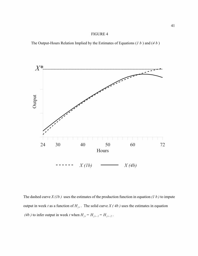
The output implications of lagged hours of work may be illustrated by comparing the

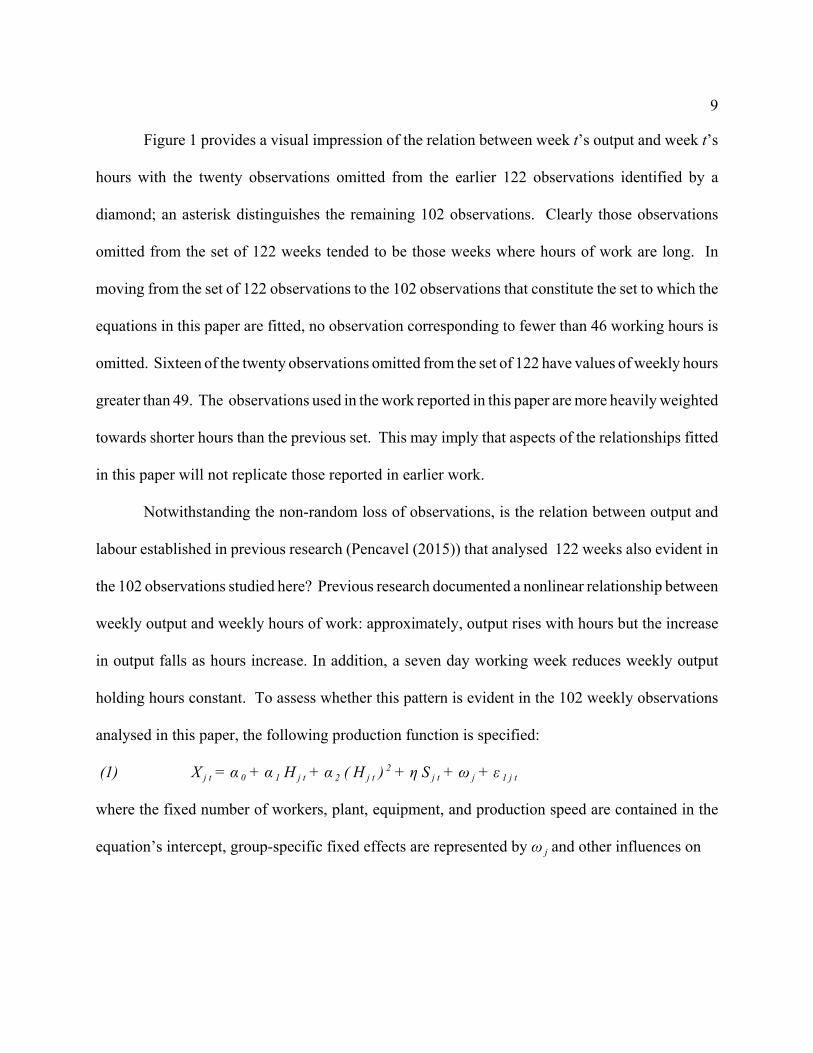
simulations of output using the estimates of equation (1b) with those of equation (4b). If a plant

manager used only contemporaneous observations on hours of work and output to infer the effects

of working hours on current output (after controlling for S j t ) and if the effects of long working

hours in previous weeks were neglected, he would use equation (1b) in Table 2 and this is graphed

in Figure 4 by the dashed curve X(1b). In Figure 4, if an output of X* were desired, the manager

would set the work schedule so that the employees would work about 70 hours. On the other hand,

if X* is the desired output for several successive weeks and if the employees worked 70 hours over

these weeks, then the relevant production function is X(4b) in Figure 4 which is the output-hours

simulation using equation (4b) when H j t = H j t-1 = H j t-2.15 When workers work at 70 hours for three

weeks and output follows the output-hours relation given by X(4b) in Figure 4, output is about 10

percent below that implied by the temporary relation graphed by X(1b).

15 In drawing the two curves in Figure 4, other variables have been held constant at the same values.

19

According to the simulation of equation X (4b), output reaches a maximum at 64 weekly

hours, a value closer to those reported in earlier research. At hours less than 64, the imputed output

corresponding to the permanent output-hours function X(4b) is little different from the

contemporaneous relation X(1b), but for hours of 64 or more the negative impact of long working

hours in previous weeks causes the predicted output of X(4b ) to lie below that of X(1b ), the gap

rising as hours increase. The use of equation (1b) to schedule hours suffers, of course, from myopia

in that the future consequences of long working hours are ignored. Compared with the permanent

output-hours relation as embodied in equation X(4b), the short-run relationship overestimates output

at 64 or more hours. The marginal product of permanent weekly hours embodied in the production

function equation (4b) declines at all hours. The average product of hours reaches a maximum at

46 hours.

To illustrate the relative effects on output in week t of the length of the working week in t

and the length of the working week in previous weeks, suppose a “long” working week is defined

as one in which 70 hours are worked in seven days while a “short” working week in one in which

40 hours are worked over six working days. The estimates reported in column (4b) of Table 5 are

used to compare the output consequences of long and short working weeks. These are reported in

the lower panel of Table 4. They resemble those reported in the upper panel of Table 4 that are

based on the estimates of equation (3a) which ignored the effects of working hours and days two

weeks earlier. Again, output in week t is more responsive to changes in the length of week t than

to variations in the lengths of weeks t - 1 and t - 2 .

20

IV. INFERENTIAL ISSUES

Previous Weeks

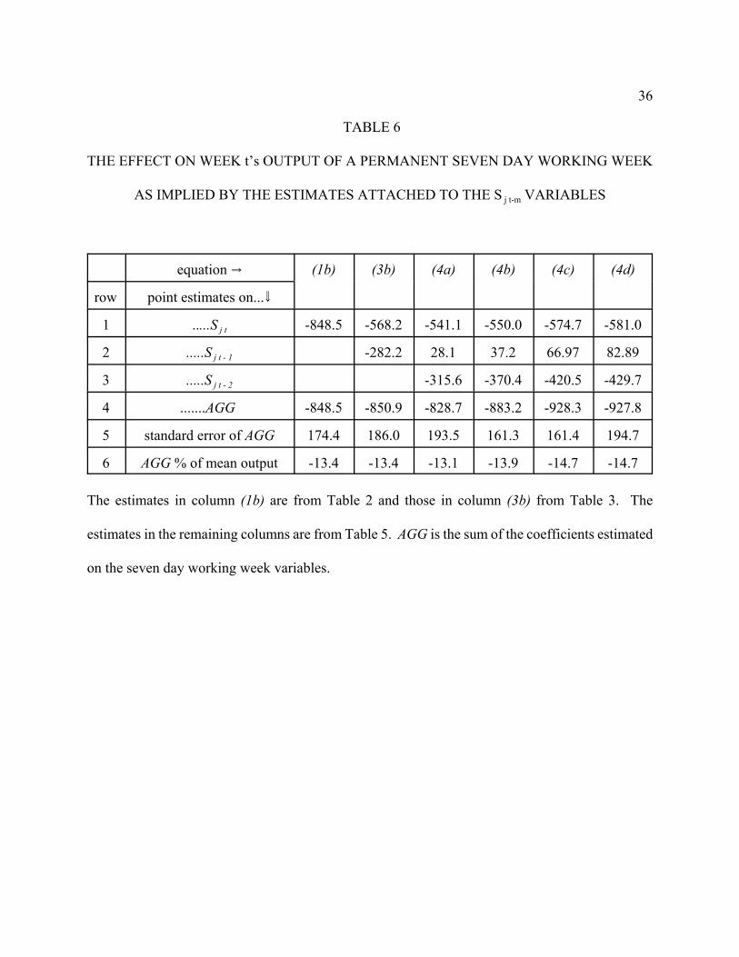
The discussion of the estimates of equation (4) in the previous section reported the joint

significance of Hj t - 2 and S j t - 2 but avoided drawing inferences about the magnitude of the effects

of individual variables. In fact, in a number of instances the coefficients attached to the variables

describing work in week t - 1 would not be judged as significantly less than zero on conventional

tests. Is it credible to accept the notion implied by the estimates of μ and ρ in Table 5 that a seven

day working week two weeks ago has more damaging effects on current output than a seven day

working week one week ago? To address these issues, consider how these values of hours and days

of work are determined.

As explained in the discussion of hours worked in Section I, weekly variations in hours

worked are proportionate to weekly variations in hours scheduled and, of course, the employer also

schedules the days of work. Therefore, it is work schedules to which we must turn to understand

the proximate determination of hours and days of work.

In this munition factory, work schedules are similar from one week to the next and, given

the necessary correlation between days and hours within each week, there is a high degree of

correlation among the right-hand side variables in equation (4). As evidence of collinearity, in these

95 weekly observations, 27 of them record S j t = S j t - 1 = S j t - 2 = 1 and 48 of them record S j t = S

j t - 1 = S j t - 2 = 0 . This high inter-correlation among the right-hand side variables is not unusual in

studies of distributed lags and, to help reduce the consequences of multicollinearity, it is common

to introduce extraneous information such as restrictions on the relative magnitudes of the

coefficients on the

21

lagged variables. Without such restrictions, unconstrained estimates are often imprecisely estimated

and result in point estimates that tend to be sensitive to small changes in equation specification.

A signal of high collinearity is provided by the point estimates on S j t - 1 that, after strongly

negative estimated coefficients in equations (2 a ) , (3 a ) , and (3 b ) of Table 3 become positive

with estimated standard errors greater than their estimated regression coefficients once variables

measuring the length of the working week in week t - 2 are introduced. However, consider a

permanent working schedule of seven working days each week so that S j t = S j t - 1 = S j t - 2 = 1 . The

effect on output in week t (other things unchanged) of a permanent seven day working schedule is

given by the sum of the coefficients on S j t , S j t - 1 , and S j t - 2 . These are reported as AGG in the

fourth row of Table 6 . Even though the separate coefficients fluctuate a good deal from row to row

in Table 6, the sum of these coefficients expressed as a percentage of mean output (in row 6)

displays less variation. The impact of a permanent change in the days of the working week is

measured with less variation than the allocation of this aggregate impact among the three weeks.

The aggregate effect is unambiguously negative and represents about 13 or 14 percent of mean

output.

Subsequent Weeks

The distinction between the temporary and permanent effects of hours and days of work on

output is not simply relevant to the interpretation of regression coefficients. It is also relevant to the

way in which hours and days of work are determined. As already noted, work schedules are not

changed frequently so that hours and days worked are similar in adjacent weeks. In these

circumstances, a permanent schedule of long hours and seven days of work with little time at the end

of the day and week to recover from work results in cumulative fatigue such that the productivity

22

of working hours and days is lower for all weeks on this schedule. If this is the case, in fitting the

production function, output in week t may be related to almost any single week on this schedule to

demonstrate an effect of long hours and days on output. To implement this hypothesis, consider the

relation between output in week t and hours and days worked in the subsequent week.

For this purpose, from the set of 122 weekly observations, another set of 95 weekly

observations is constructed that contains information on X j t , H j t , H j t + 1 , H j t + 2 , S j t , S j t + 1 , and

S j t + 2 . This is not the same set of weeks on the dependent variable as the 95 weeks that contained

information on H j t , H j t - 1 , H j t - 2 , S j t , S j t - 1 , and S j t - 2 although the two sets intersect : of the 95

weekly observations with information on hours and days worked in weeks t , t + 1 , and t + 2, 81

of them also appear in the 95 observations with information on work in weeks t , t - 1 , and t - 2 .

To help distinguish the two sets of observations, those used in the previous section using hours and

days worked in t - 1 and t - 2 are denoted 95LAG and those used immediately below with hours and

days in weeks t + 1 and t + 2 are called 95LEAD. Descriptive statistics on 95LEAD are provided

in the bottom panel of Table 1. The weeks constituting observations on H j t - 1 and S j t - 1 in 95LAG

are the same as those weeks constituting H j t + 1 and S j t + 1 in 95LEAD though the weeks that make

up the observations on X j t are different.

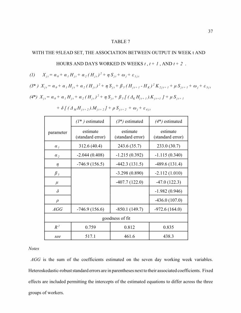
First, with the observations in 95LEAD, equation (1) was estimated; this relates output in

week t to hours and days worked in week t . The least-squares estimates are given in the column

headed “(1 ) estimated” of Table 7 and they yield similar inferences to those in the set of 95LAG.

23

Now estimate equation (3) with H t - 1 replaced by H t + 1 and with S t - 1 replaced by S t + 1 :

(3* ) X j t = α 0 + α 1 H j t + α 2 ( H j t ) 2 + η S j t + β 5 ( H j t + 1 - H K ) 2 K 2 j t + 1 + μ S j t + 1 + ω j + ε 3 j t

where, as before, the knot H K is set to 53 and K 2 j t + 1 equals unity when H j t + 1 $53 and is zero

otherwise.

Also estimate equation (4) with H t - 1 replaced by H t + 1, H t - 2 replaced by H t + 2 , S t - 1

replaced by S t + 1 , and S t - 2 replaced by S t + 2 :

(4* ) X j t = α 0 + α 1 H j t + α 2 ( H j t )2 + η S j t + β 5 [ ( ΔK Hj t + 1 ).K j t +1 ] + μ S j t + 1

+ δ [ ( Δ M Hj t + 2 ).M j t +2 ] + ρ S j t + 2 + ω j + ε 4 j t

where ΔK Hj t + 1 = ( H j t + 1 - 53 ) 2 and K j t +1 = 1 if H j t + 1 $ 53 and is zero otherwise; and

Δ M Hj t + 2 = ( H j t + 2 - 55 ) 2 and M j t +2 = 1 if Hj t + 2 $ 55 and is zero otherwise.

The least-squares estimates of equations (3*) and (4* ) are given in columns headed “(3*)

estimated” and “(4*) estimated” respectively in Table 7. The estimates of equations (3*) and (4*)

in Table 7 in which output is related to hours and days worked in weeks t , t +1 , and t + 2 are

similar to those of equation (3b) of Table 3 and (4b) of Table 5. Why should this be the case?

Because adjacent weeks differ little in their length and, given a well-defined production

function with other inputs constant, working weeks of similar length will yield similar outputs.

Adjacent weeks are similar in length because work schedules change infrequently.

As examples, for the 100 women turning fuze bodies, consider the weeks between the

beginning of February to early June in 1916: there are 14 working weeks in this period not counting

the Easter break (and two weeks where hours were cut because of a shortage of raw material) and,

of these 14 weeks, 10 of them schedule a working week of exactly 66.5 hours (ten hours a day for

six days and the remainder on Sunday). Then, from early September to mid-December 1916, there

24

are 16 working weeks and 10 of them schedule a working week of 58.5 hours (ten hours a day, the

remainder on Saturday with no Sunday work). Every week from November 1915 to the end of April

1916 was a seven day working week and every week from mid-August to end December 1916 was

a six day working week. In circumstances such as these, a sequence of weeks with long work

schedules result in cumulative fatigue at work and in inadequate time to recuperate from work so

the damaging effects of long working weeks is exhibited in any single week.

V. CONCLUSION

Using the equivalent of almost two years of weekly observations, this paper has presented

evidence suggesting that the damaging effects for workers’ performance of long hours and days

extend beyond the week in which these hours and days are worked. When a succession of long

working weeks or days are scheduled and adequate time for rejuvenation denied, cumulative fatigue

is apt to result.

What constitutes a long working week? In the particular setting of these munition workers,

other things constant, seven days of work and hours beyond 53 weekly hours in the previous week

have negative consequences for output in the following week. Indeed, there is evidence of damaging

effects on a week’s output of a long working week hours (in this study, weekly hours beyond 55 and

a seven day week) two weeks previously. These thresholds are approximate and have not been

estimated precisely. They may well be different for other workers and other jobs.

Just as machines tend to depreciate with use over time and need repair and maintenance to

ensure their value in production so also labor requires repair and recovery from work to maintain

its productivity at the workplace : a long working week calls for a longer time for repair, but a

continuous schedule of long working weeks in succession does not permit workers the necessary

25

restoration and, without repair, ultimately, health and work productivity may suffer.16

The importance for output of the elimination of a seven day work week speaks to the

distinction between the effects of a shorter work day and the impact of an entire day of rest. There

is some suggestion in the writings of the investigators of the Health of Munition Workers Committee

that not only were there immediate benefits to shorter hours but also longer run advantages as

workers fully adjusted to a shorter working week that involved a restorative day of rest. That is, lags

in the effects of hours reductions on output have been reported in cases where many weeks of

successive long hours required correspondingly many weeks of shorter hours before the full effects

on increased output were revealed.17 In the words of one economist, “It takes time for the beneficial

effects of an hours reduction upon the productivity of workers to appear in a company’s profit

account” (Lester, 1941, p.70). This gives rise to intertemporal relations in the production function

such that the extent to which an input is used in one period has consequences for output in another

period.

This link between a succession of long working weeks and output in these weeks would not

surprise some earlier observers. For instance, in calling for shorter hours of work, the Health of

Munition Workers Committee (1919, ¶ 162, p. 40) recognised that, not only would this have

16 Long hours of work have adverse effects not only on productivity in the workplace but also on the

quality of home life. See White et al. (2003).

17 An example is provided by a four year study of open-hearth steel furnaces: after two years of

observation of workers on a twelve hours a day schedule, hours were cut to eight hours. Although

monthly output per hour started to rise immediately, the full maximum recovery in output was not

reached until 13 months after the initial hours reduction. See Vernon (1921, pp. 36-8).

26

desirable effects on the employer’s costs, but also “....a longer period is left for recovery, for the

enjoyment of adequate sleep and rest, and for the necessary opportunity for recreation, exercise, and

the discharge of the ordinary duties of citizenship and domestic life.”

The relevance of the need for recovery from work may help to explain the comparative work

performance of night work and day work. The Health of Munition Workers Committee determined

that the output of workers employed each and every week on night shifts was “very unfavourable”

to that of day workers because night work required workers to sleep and recuperate during the day

and such recovery was more difficult to obtain at that time. However, when workers were on a

discontinuous system alternating between one week on a day schedule and the following week on

a night schedule, the Committee found there was “no significant difference between the rate of

output in night and day shifts........If there be any difference, it would seem that the output is slightly

better by night for the particular class of work involved.”18

This slight superiority of night work on the discontinuous system might reflect the

incomplete recovery that day workers realised from last week’s night work. That is, if the

Committee are correct in maintaining that night work allows for less sleep and recovery from work

than day work, then this week’s night workers were working during the day last week and recovered

more fully from last week’s work.

It is obvious that the circumstances and setting of the observations examined in this paper

are unusual. Whether the findings in this paper can be extended to other workplaces in more recent

settings is a topic for future research. The principal hypothesis to be examined is that a work

18 The composition of the night workers and the day workers on these discontinuous shifts was,

therefore, the same. See HMWC (1916, pp. 26-40).

27

schedule that involves a sequence of long working weeks or days and that allows little time for

recovery from work tends to result in immoderate fatigue that affects work performance.

28

REFERENCES

CONWAY, S.H., L.POMPEII, R.E.ROBERTS, J.L.FOLLIS, and GIMENO, D. (2016). Dose-

response relation between work hours and cardiovascular disease risk. Journal of Occupational and

Environmental Medicine, 58 (3) , 221-26.

FRITZ, C. and SONNENTAG., S.(2006). Recovery, well-being, and performance-related outcomes:

the role of workload and vacation experiences. Journal of Applied Psychology, 91(4), 936-45.

FRITZ, C., SONNENTAG, S., SPECTOR,P. and MCINROE, J. (2010). The weekend matters:

relationships between stress recovery and affective experiences. Journal of Organizational

Behavior, 31 , 1137-62.

GOLDEN, L. (2012). The effects of working time on productivity and firm performance: a research

synthesis paper. Conditions of Work and Employment Branch, Series No. 33, International Labour

Office: Geneva.

HEALTH OF MUNITION WORKERS COMMITTEE (GREAT BRITAIN MINISTRY OF

MUNITIONS) (1916) Memorandum No. 12 Statistical Information Concerning Output in Relation

to Hours of Work. London Cd. 8344

___ (1919). Final Report. London: Cmd. 9065

29

HICKS, J.R. (1932). The Theory of Wages. London: Macmillan.

HULST, M. van der (2003). Long workhours and health. Scandinavian Journal of Work,

Environment and Health, 29(3): 171-88.

JACOBSEN, H. B., REME, S.E., SEMBAJWE, G., HOPCIA, K., STILES, T.C., SORENSEN, G.,

PORTER, J.H., MARINO, M. and BUXTON, O.M. (2014) . Work stress, sleep deficiency, and

predicted 10-year cardiometabolic risk in a female patient care worker population. American

Journal of Industrial Medicine 57(8) , 940-49.

JANSEN, N. , KANT, I. and VAN DEN BRANDT, P.A. (2002). Need for recovery in the working

population: description and associations with fatigue and psychological distress. International

Journal of Behavioral Medicine, 94(4), 322-40.

KEEGAN, J. (1999) The First World War New York: Alfred A. Knopf.

LESTER, R. (1941) Economics of Labor New York: Macmillan.

NYLAND, C. (1989). Reduced worktime and the management of production. Cambridge:

Cambridge University Press.

30

PENCAVEL, J. (2015).The productivity of working hours. The Economic Journal 125(589), 2052-

76.

SONNENTAG, S. and ZIJLSTRA, F.(2006) Job characteristics and off-job activities as predictors

of need for recovery, well-being, and fatigue. Journal of Applied Psychology 91 (2), 330-50.

VERNON, H.M. (1921) Industrial fatigue and efficiency. London: George Routledge.

WESTMAN, M., and ETZION, D., (2001). The impact of vacation and job stress on burnout and

absenteeism. Psychology and Health 16 (5), 595-606.

WHITE, M. HILL, S., MCGOVERN, P., MILLS, C. and SMEATON, D. (2003). High Performance

Management Practices, Working Hours and Work-Life Balance. British Journal of Industrial

Relations 41 (2), 175-95.

31

TABLE 1

DESCRIPTIVE STATISTICS ON THREE SETS OF WEEKLY OBSERVATIONS CONTAINING

INFORMATION ON HOURS AND DAYS OF WORK IN ADJACENT WEEKS

mean minimum 1st quartile median 3rd quartile maximum standard

deviation

102 weekly observations on weeks t and t - 1

X (j , t ) 6,333 2,919 5,708 6,696 7,092 8,735 1,210

H (j, t ) 50.3 24.0 46.0 50.1 55.8 71.8 10.1

H (j, t-1 ) 51.4 24.0 47.5 50.6 56.1 71.8 9.4

The mean value of S( j , t ) is 0.37 and that of S( j , t - 1 ) is 0.40.

95 weekly observations on weeks t, t - 1, and t-2 ; 95LAG

X (j , t ) 6,329 2,919 5,708 6,521 7,135 8,735 1,225

H (j, t ) 50.0 24.0 46.0 49.9 55.6 71.8 10.1

H (j, t-1 ) 51.2 24.0 46.9 50.6 56.1 71.8 9.5

H (j, t-2 ) 52.0 24.0 47.6 50.7 56.2 71.8 8.9

The mean value of S( j , t ) is 0.36, that of S( j , t - 1 ) is 0.40, and that of S( j , t - 2) is 0.41.

95 weekly observations on weeks t , t + 1 , and t + 2 ; 95LEAD

X (j , t ) 6,482 2,919 5,985 6,783 7,092 8,491 1,025

H (j, t ) 52.0 24.0 47.6 50.7 56.2 71.8 8.9

H (j, t+1) 51.2 24.0 46.9 50.6 56.1 71.8 9.5

H (j, t+2) 50.0 24.0 46.0 49.9 55.6 71.8 10.1

The mean value of S( j , t ) is 0.41, that of S( j , t + 1 ) is 0.39, and that of S( j , t + 2) is 0.36.

32

TABLE 2

ESTIMATED EFFECTS OF WEEK t’s WORKING HOURS AND DAYS ON OUTPUT IN t

(1) X j t = α 0 + α 1 H j t + α 2 ( H j t ) 2 + η S j t + ω j + ε j t

( 1 a ) ( 1 b )

nobs 102 95

parameter estimate (standard error) estimate (standard error)

α 1 282.0 (30.6) 271.1 (30.4)

α 2 -1.745 (0.346) -1.616 (0.350)

η - 784.5 (168.3) -848.5 (174.5)

goodness of fit statistics

R2 0.803 0.803

see 551.5 558.7

Notes

Estimated standard errors in parentheses are heteroskedastic-robust. see is the standard error of

estimate of the fitted equation. Fixed effects are included that allow the intercepts of the fitted

equations to be different for the three groups of workers. nobs means number of observations.

33

TABLE 3

ESTIMATED EFFECTS OF LAGGED HOURS & DAYS OF WORK ON CURRENT OUTPUT

(2) X j t = α 0 + α 1 H j t + α 2 ( H j t ) 2 + η S j t + [ β 0 + β 1 (H j t - 1 - H o ) + β 2 ( H j t - 1 - H o )

2] K 1 j t - 1

+ [ β 3 + β 4 (H j t - 1 - H K ) + β 5 ( H j t - 1 - H K ) 2] K 2 j t - 1 + μ S j t - 1 + ω j + ε 2 j t

(3) X j t = α 0 + α 1 H j t + α 2 ( H j t ) 2 + η S j t + β 5 ( H j t - 1 - H K ) 2 K 2 j t - 1 + μ S j t - 1 + + ω j + ε 3 j t

equation (2) estimated equation (3) estimated

( 2 a ) ( 3 a ) ( 3 b )

nobs 102 102 95

parameter estimate (standard error) estimate (standard error) estimate (standard error)

α 1 233.9 (29.4) 238.6 (28.8) 222.7 (27.4)

α 2 -1.184 (0.338) -1.203 (0.333) -1.032 (0.320)

η -537.2 (167.1) -518.2 (164.7) -568.2 (172.2)

β 1 18.9 (28.5) 0 0

β 2 -0.21 (0.81) 0 0

β 4 6.76 (20.4) 0 0

β 5 -3.17 (1.35) -2.73 (0.64) -2.91 (0.65)

μ -309.4 (141.9) -282.2 (121.6) -282.6 (137.3)

R2 0.832 0.828 0.831

see 520.0 519.6 523.6

Notes Estimated standard errors in parentheses are heteroskedastic-robust. see is the standard error

of estimate of the fitted equation. Fixed effects are included that allow the intercepts of the fitted

equations to be different for the three groups of workers. nobs means number of observations. In

these estimates, H o is 24 hours and the knot H K is 53 hours. In columns (3a) and ( 3b ), there is no

effect of hours in week t - 1 on output in week t until H j t - 1 exceeds the knot.

34

TABLE 4

CONSEQUENCES FOR THE CURRENT WEEK’S OUTPUT OF CURRENT AND LAGGED

SHORT AND LONG WORKING WEEKS AS IMPLIED BY EQUATIONS (3a) AND (4b)

Using Equation (3 a)

current week

short long Δ

previous

week

short 100 135 } 35long 86 121

Δ -14

Using Equation (4 b)

current week

short long Δ

previous

weeks

short 100 142.8 } 42.8long 79 121.8

Δ -21

Notes

Δ denotes the difference in output between a “long” working week and a “short” working week.

A short working week (both current and previous) is defined as one when H = 40 and S = 0.

A long working week (both current and previous) is defined as one when H = 70 and S = 1 . The

output corresponding to the case in which both week t and the previous weeks t - 1 and t-2 are short

working weeks constitutes the reference output with which the other outputs are compared.

35

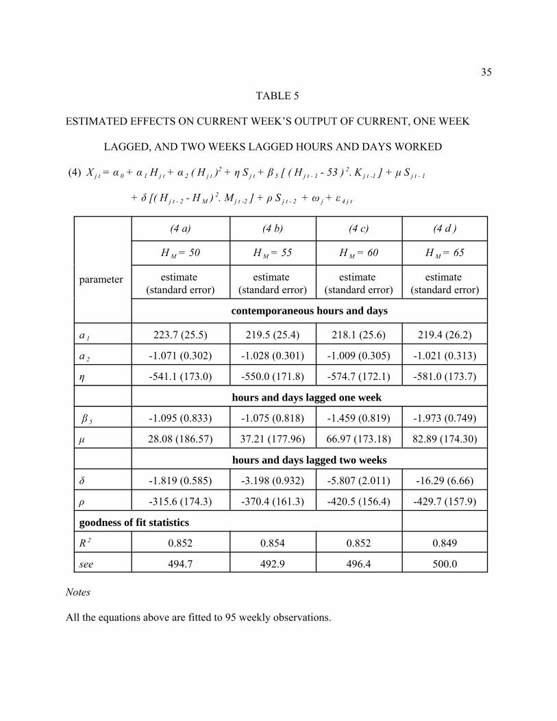
TABLE 5

ESTIMATED EFFECTS ON CURRENT WEEK’S OUTPUT OF CURRENT, ONE WEEK

LAGGED, AND TWO WEEKS LAGGED HOURS AND DAYS WORKED

(4) X j t = α 0 + α 1 H j t + α 2 ( H j t )2 + η S j t + β 5 [ ( H j t - 1 - 53 ) 2. K j t -1 ] + μ S j t - 1

+ δ [( H j t - 2 - H M ) 2. M j t -2 ] + ρ S j t - 2 + ω j + ε 4 j t

parameter

(4 a) (4 b) (4 c) (4 d )

H M = 50 H M = 55 H M = 60 H M = 65

estimate (standard error)

estimate (standard error)

estimate (standard error)

estimate (standard error)

contemporaneous hours and days

a 1 223.7 (25.5) 219.5 (25.4) 218.1 (25.6) 219.4 (26.2)

a 2 -1.071 (0.302) -1.028 (0.301) -1.009 (0.305) -1.021 (0.313)

η -541.1 (173.0) -550.0 (171.8) -574.7 (172.1) -581.0 (173.7)

hours and days lagged one week

β 5 -1.095 (0.833) -1.075 (0.818) -1.459 (0.819) -1.973 (0.749)

μ 28.08 (186.57) 37.21 (177.96) 66.97 (173.18) 82.89 (174.30)

hours and days lagged two weeks

δ -1.819 (0.585) -3.198 (0.932) -5.807 (2.011) -16.29 (6.66)

ρ -315.6 (174.3) -370.4 (161.3) -420.5 (156.4) -429.7 (157.9)

goodness of fit statistics

R 2 0.852 0.854 0.852 0.849

see 494.7 492.9 496.4 500.0

Notes

All the equations above are fitted to 95 weekly observations.

36

TABLE 6

THE EFFECT ON WEEK t’s OUTPUT OF A PERMANENT SEVEN DAY WORKING WEEK

AS IMPLIED BY THE ESTIMATES ATTACHED TO THE S j t-m VARIABLES

equation Y (1b) (3b) (4a) (4b) (4c) (4d)

row point estimates on...\

1 .....S j t -848.5 -568.2 -541.1 -550.0 -574.7 -581.0

2 .....S j t - 1 -282.2 28.1 37.2 66.97 82.89

3 .....S j t - 2 -315.6 -370.4 -420.5 -429.7

4 .......AGG -848.5 -850.9 -828.7 -883.2 -928.3 -927.8

5 standard error of AGG 174.4 186.0 193.5 161.3 161.4 194.7

6 AGG % of mean output -13.4 -13.4 -13.1 -13.9 -14.7 -14.7

The estimates in column (1b) are from Table 2 and those in column (3b) from Table 3. The

estimates in the remaining columns are from Table 5. AGG is the sum of the coefficients estimated

on the seven day working week variables.

37

TABLE 7

WITH THE 95LEAD SET, THE ASSOCIATION BETWEEN OUTPUT IN WEEK t AND

HOURS AND DAYS WORKED IN WEEKS t , t + 1 , AND t + 2 .

(1) X j t = α 0 + α 1 H j t + α 2 ( H j t ) 2 + η S j t + ω j + ε 1 j t

(3* ) X j t = α 0 + α 1 H j t + α 2 ( H j t ) 2 + η S j t + β 5 ( H j t + 1 - H K ) 2 K 2 j t + 1 + μ S j t + 1 + ω j + ε 3 j t

(4*) X j t = α 0 + α 1 H j t + α 2 ( H j t ) 2 + η S j t + β 5 [ ( ΔK Hj t + 1 ).K j t +1 ] + μ S j t + 1

+ δ [ ( Δ M H j t + 2 ).M j t + 2 ] + ρ S j t + 2 + ω j + ε 4 j t

parameter

(1* ) estimated (3*) estimated (4*) estimated

estimate(standard error)

estimate(standard error)

estimate(standard error)

α 1 312.6 (40.4) 243.6 (35.7) 233.0 (30.7)

α 2 -2.044 (0.408) -1.215 (0.392) -1.115 (0.340)

η -746.9 (156.5) -442.3 (131.5) -489.6 (131.4)

β 5 -3.298 (0.890) -2.112 (1.010)

μ -407.7 (122.0) -47.0 (122.3)

δ -1.982 (0.946)

ρ -436.0 (107.0)

AGG -746.9 (156.6) -850.1 (149.7) -972.6 (164.0)

goodness of fit

R 2 0.759 0.812 0.835

see 517.1 461.6 438.3

Notes

AGG is the sum of the coefficients estimated on the seven day working week variables.

Heteroskedastic-robust standard errors are in parentheses next to their associated coefficients. Fixed

effects are included permitting the intercepts of the estimated equations to differ across the three

groups of workers.

38

FIGURE 1

Output and Hours Worked in Week t Identifying the 20 Observations Omitted from the Set of 122

Weeks to Form the 102 Weeks Used for the Analysis in this Paper

The asterisks denote the observations in the set of 122 weeks previously analysed. The diamond

identifies the 20 observations omitted that result in the 102 weekly observations used in this

analysis.

39

FIGURE 2

The Relation between Hours Worked in Week t and

Hours Worked in Week t - 1

40

FIGURE 3

The Relation between Output in Week t and Hours Worked in Week t - 1 as Implied by the

Estimates of the Spline Function in Lagged Hours in Table 3

X(Q - Q) corresponds to the spline where the output-hours relation takes the form of a quadratic in

both regimes as in equation (2 a ) . X(0 - Q) is the spline where output is invariant to hours in the

shorter hours regime as in equation ( 3 a ). The two curves are drawn holding H j t , and S j t constant

at the same values.

41

FIGURE 4

The Output-Hours Relation Implied by the Estimates of Equations (1 b ) and (4 b )

The dashed curve X (1b ) uses the estimates of the production function in equation (1 b ) to impute

output in week t as a function of H j t . The solid curve X ( 4b ) uses the estimates in equation

(4b ) to infer output in week t when H j t = H j t - 1 = H j t - 2 .