Embed Size (px)
Citation preview

Recurrent Networks Rooted in Statistical Physics
8.1 Introduction The multilayer perceptron and the radial-basis function network considered in the previous two chapters represent important examples of a class of neural networks known as nonlinear layered feedforward networks. In this chapter we consider another important class of neural networks that have a recurrent structure, and the development of which is inspired by different ideas from statistical physics. In particular, they share the following distinctive features:
8 Nonlinear computing units
8 Symmetric synaptic connections
8 Abundant use of feedback
All the characteristics described herein are exemplified by the Hopfield network, the Boltzmann machine, and the mean-field-theory machine.
The Hopfield network is a recurrent network that embodies a profound physical princi- ple, namely, that of storing information in a dynamically stable conjiguration. Prior to the publication of Hopfield’s influential paper in 1982, this approach to the design of a neural network had occupied the attention of several investigators-Grossberg (1967, 1968), Amari (1972), Little (1974), and Cowan (1968), among others; the work of some of these pioneers predated that of Hopfield by more than a decade. Nevertheless, it was in Hopfield’s 1982 paper that the physical principle of storing information in a dynamically stable network was formulated in precise terms for the first time. Hopfield’s idea of locating each pattern to be stored at the bottom of a “valley” of an energy landscape, and then permitting a dynamical procedure to minimize the energy of the network in such a way that the valley becomes a basin of attraction is novel indeed!
The standard discrete-time version of the Hopfield network uses the McCulloch-Pitts model for its neurons. Retrieval of information stored in the network is accomplished via a dynamical procedure of updating the state of a neuron selected from among those that want to change, with that particular neuron being picked randomly and one at a time. This asynchronous dynamical procedure is repeated until there are no further state changes to report. In a more elaborate version of the Hopfield network, the firing mechanism of the neurons (Le., switching them on or off) follows aprobabilistic law. In such a situation, we refer to the neurons as stochastic neurons. The use of stochastic neurons permits us to develop further insight into the statistical characterization of the Hopfield network by linking its behavior with the well-established subject of statistical physics.
The Boltzmann machine represents a generalization of the Hopfield network (Hinton and Sejnowski, 1983,1986; Ackley et al., 1985). It combines the use of symmetric synaptic
285
286 8 / Recurrent Networks Rooted in Statistical Physics
connections (a distinctive feature of the Hopfield network) with the use of hidden neurons (a distinctive feature of multilayer feedforward networks). For its operation, the Boltzmann machine relies on a stochastic concept rooted in statistical thermodynamics that is known as simulated annealing (Kirkpatrick et al., 1983). The Boltzmann machine was named by Hinton and Sejnowski in honor of Boltzmann. The general discipline of statistical thermodynamics grew out of the work of Boltzmann who, in 1872, made the discovery that the random motion of the molecules of a gas has an energy related to temperature.
The mean-field-theory (MFT) machine is derived from the Boltzmann machine by invoking a “naive” approximation known as the mean-field approximation (Peterson and Hartman, 1989; Peterson and Anderson, 1987). According to this approximation, the stochastic binary units of the Boltzmann machine are replaced by deterministic analog units. The motivation for the mean-field approximation is to circumvent the excessive computer time required for the implementation of the Boltzmann machine.
The Hopfield network operates in an unsupervised manner. As such, it may be used as a content-addressable memory or as a computer for solving optimization problems of a combinatorial kind. In a combinatorial optimization problem we have a discrete system with a large but finite number of possible solutions; the requirement is to find the solution that minimizes a cost function providing a measure of system performance. The Boltzmann machine and its derivative, the mean-field-theory machine, on the other hand, may require supervision by virtue of using input and output units.
The Hopfield network, the Boltzmann machine, and the mean-field-theory machine require time to settle to an equilibrium condition; they may therefore be excessively slow, unless special-purpose chips or hardware are used for their implementation. Moreover, they are relaxation networks with a local learning rule. Above all, however, they are all rooted in statistical physics.
Organization of the Chapter
The main body of this chapter is organized as follows. In Section 8.2 we present an overview of the dynamics of the class of recurrent networks considered here. In Section 8.3 we describe the Hopfield network, which uses the formal neuron of McCulloch and Pitts (1943) as its processing unit. The convergence properties of the Hopfield network are given particular attention here. This is followed by a computer experiment illustrating the behavior of the Hopfield network in Section 8.4. Then, in Section 8.5, we discuss the energy function of the Hopfield network and the related issue of spurious states. In Section 8.6 we present a probabilistic treatment of associative recall in a Hopfield network. The material covered in this latter section establishes a fundamental limit on the storage capacity of the Hopfield network as an associative memory for correlated patterns. In Section 8.7 we discuss the “isomorphism” between the Hopfield network and the spin- glass model that is rooted in statistical mechanics. This is followed by a description of stochastic neurons in Section 8.8, and then a qualitative discussion of the phase diagram of a stochastic Hopfield network in Section 8.9. The phase diagram delineates the lines across which the network changes its computational behavior.
In Section 8.10 we describe the stochastic simulated annealing algorithm. This material paves the way for a detailed description of the Boltzmann machine in Section 8.11 from a statistical physics perspective. In Section 8.12 we view the Boltzmann machine as a Markov chain model. Next, we describe the mean-field-approximation theory in Section 8.13. In Section 8.14 we describe a computer experiment comparing the Boltzmann and mean-field-theory machines. The chapter concludes with some general discussion in Sec- tion 8.15.

8.2 I Dynamical Considerations 287
8.2 Dynamical Considerations Consider a recurrent network (i.e., a neural network with feedback) made up of N neurons with symmetric coupling described by w,, = w , ~ , where w,, is the synaptic weight connecting neuron i to neuron j . The symmetry of the synaptic connections results in a powerful theorem about the behavior of the network, as discussed here. Let u,(t) denote the activation potential acting on neuron j , and let x,(t) denote the corresponding value of the neuron's output. These two variables are related by
xj = PJ(u,> (8.1)
where p,(.) is the sigmoidal nonlinearity of neuron j . Both u, and x, are functions of the continuous-time variable t. The state of neuronj may be described in terms of the activation potential u,(t) or, equivalently, the output signal x,(t). In the former case, the dynamics of the recurrent network is described by a set of coupled nonlinear differential equations as follows (Hopfield, 1984a; Cohen and Grossberg, 1983):
(8.2)
where 0, is a threshold applied to neuronj from an external source. The finite rate of change of the activation potential uj(t) with respect to time t is due to the capacitive effects Cj associated with neuron j , which are an intrinsic property of biological neurons or the physical implementation of artificial neurons. According to Eq. (8.2), three factors contribute to the rate of change dujldt:
1. Postsynaptic effects induced in neuron j due to the presynaptic activities of neurons
2. Leakage due to finite input resistance Rj of the nonlinear element of neuron j 3. Threshold 0,
i = 1, 2, . . . , N , excluding i = j
For the recurrent network with symmetric coupling as described here, we may define an energy function or Liapunou function as follows (Hopfield, 1984a):
where xj is the output of neuronj, related to the activation potential uj by Eq. (8.1). The energy function of Eq. (8.3) is a special case of a theorem due to Cohen and Grossberg (1983), which is considered in Chapter 14 devoted to neurodynamics. The importance of the energy function E is that it provides the basis for a deep understanding of how specific problems may be solved by recurrent networks. For now, it suffices to note that the energy function E is fully descriptive of the recurrent network under study in that it includes all the synaptic weights and all the state variables of the network, and that we may state the following theorem for the case when the threshold 4 changes slowly over the time of computation (Hopfield, 1984a; Cohen and Grossberg, 1983):
The energy function E is a monotonically decreasing function of the network state {xj l j = 1, 2 , . . . , N}.
When the network is started in any initial state, it will move in a downhill direction of the energy function E until it reaches a local minimum; at that point, it stops changing
288 8 / Recurrent Networks Rooted in Statistical Physics
with time. Simply put, a recurrent network with symmetric coupling cannot oscillate despite the abundant presence of feedback.
We refer to the space of all possible states of the network as the phase space, a terminology borrowed from physics; it is also referred to as the state space. The local minima of the energy function E represent the stable points of the phase space. These stable points are also referred to as attractors in the sense that each attractor exercises a substantial domain of influence (Le., basin of attraction) around it. Accordingly, symmetric recurrent networks are sometimes referred to as attractor neural networks (Amit, 1989).
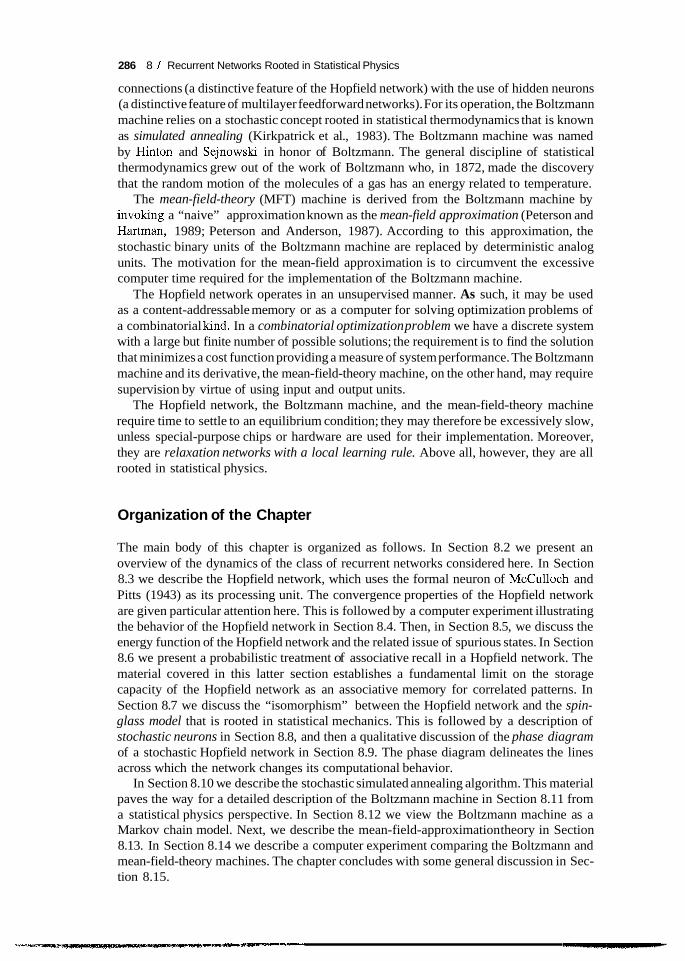
Figure 8.1 presents a graphical portrayal of the above theorem for a two-dimensional phase space (Hopfield and Tank, 1986). Each trajectory of the $ow map shown in Fig. 8.lb corresponds to a possible time history of the network, with arrows indicating the directions of motion. Each trajectory terminates at a stable point, which is due to the network moving in a downhill direction of the energy function E toward the bottom of a local valley and then stopping there. Figure 8.la shows the energy landscape for the flow map of Fig. 8. lb. Each contour line of the energy landscape corresponds to a constant
(C)
FIGURE 8.1 indicate a hill, whereas dashed lines indicate a valley. (b) Flow lines of the network dynamics, corresponding to the energy landscape (a). (c) More complicated dynamics that can occur for an asymmetric recurrent network. (From J.J. Hopfield and T.W. Tank, 1986; copyright 1986 by the AAAS.)
(a) Energy landscape of a symmetric recurrent network; solid lines

8.3 / The Hopfield Network 289
value of the energy function E. The solid contour lines of Fig. 8.la indicate hills, whereas the dashed contour lines indicate valleys. The bottom points of the valleys represent stable points of the phase space; that is, the valleys are located where the trajectories in Fig. 8.lb terminate. When the network is presented a pattern that is inside the domain of influence of an attractor of the phase space, the network relaxes to that attractor, as illustrated in the bottom left-hand corner of Fig. 8.la.
The picture portrayed by the flow map of Fig. 8.lb corresponds to a recurrent network with symmetric coupling. What if the coupling is asymmetric? In such a situation it is possible for complications to arise, as illustrated in the flow map of Fig. 8.lc, which exhibits trajectories representative of complicated oscillatory behaviors (Hopfield and Tank, 1986). It is important to recognize, however, that it is possible to design stable recurrent networks that are asymmetric (Carpenter et al., 1987). Nevertheless, the use of symmetric coupling does indeed help by simplifying the class of behaviors that are exhibited by neural networks having feedback. It is for this reason that in this chapter we focus our attention exclusively on recurrent networks that are symmetric. A simple and yet important example of this special class of recurrent networks is represented by the Hopfield network, which is considered next.
8.3 The Hopfield Network
The Hopfield network may bg viewed as a nonlinear associative memory or content- addressable memory, the primary function of which is to retrieve a pattern (item) stored in memory in response to the presentation of an incomplete or noisy version of that pattern. To illustrate the meaning of this statement in a succinct way, we can do no better than quote from the 1982 paper of Hopfield:
Suppose that an item stored in memory is “H.A. Kramers & G.H. Wannier Physi Rev. 60, 252 (1941).” A general content-addressable memory would be capable of retrieving this entire memory item on the basis of sufficient partial information. The input “& Wannier (1941)” might suffice. An ideal memory could deal with errors and retrieve this reference even from the input “Wannier, (1941).”
An important property of a content-addressable memory is therefore the ability to retrieve a stored pattern, given a reasonable subset of the information content of that pattern. Moreover, a content-addressable memory is error-correcting in the sense that it can override inconsistent information in the cues presented to it.
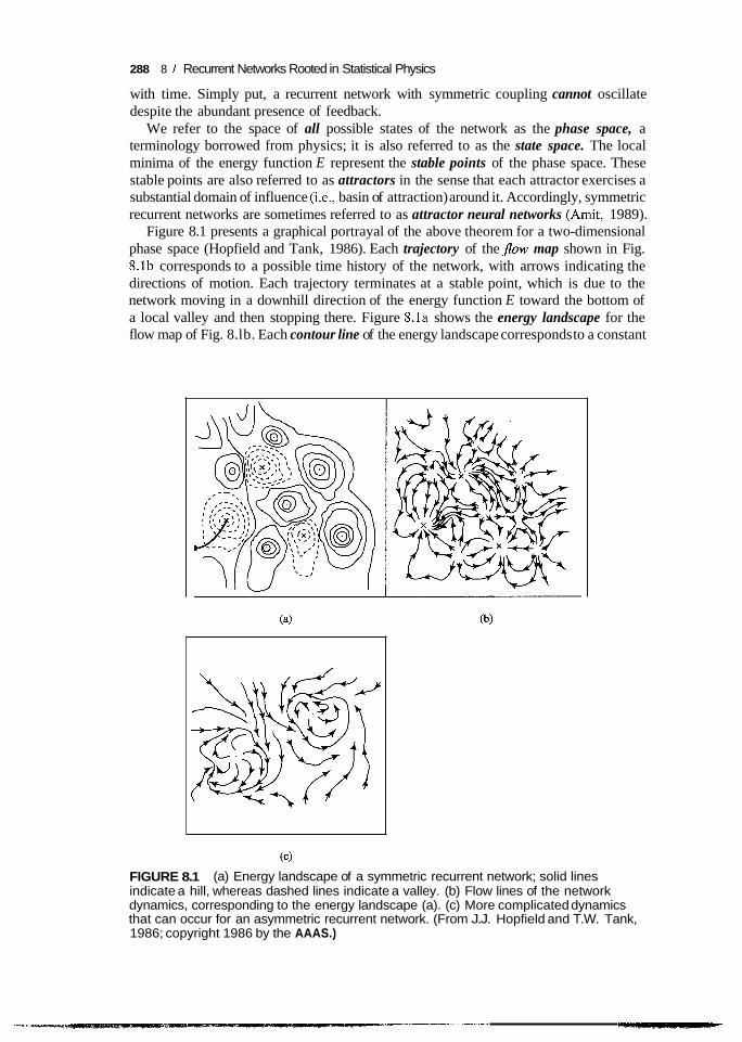
The essence of a content-addressable memory (CAM) is to map a fundamental memory E,, onto a fixed (stable) point s, of a dynamic system, as illustrated in Fig. 8.2. Mathemati- cally, we may express this mapping in the form
E, e s, The arrow from left to right describes an encoding operation, whereas the arrow from right to left describes a decoding operation. The stable points of the phase space of the network are the fundamental memories or prototype states of the network. Suppose now that the network is presented a pattern containing partial but sufficient information about one of the fundamental memories. We may then represent that particular pattern as a starting point in the phase space. In principle, provided that the starting point is close to the stable point representing the memory being retrieved, the system should evolve with
290 8 / Recurrent Networks Rooted in Statistical Physics
Decoding w-7 fundamental
memories
stored vectors
FIGURE 8.2 Illustration of the coding-decoding performed by a recurrent network.
time and finally converge onto the memory state itself, at which point the entire memory is generated by the network. We may therefore describe a Hopfield network as a dynamic system whose phase space contains a set offuced (stable) points representing thefundamen- tal memories of the system. Consequently, the Hopfield network has an emergent property, which helps it retrieve information and cope with errors.
Operational Features of the Hopfield Network
The Hopfield model uses the formal neuron of McCulloch and Pitts (1943) as its basic processing unit. Each such neuron has two states determined by the level of the activation potential acting on it. The “on” or “firing” state of a neuron i is denoted by the output si = f l , and the “off” or “quiescent” state is represented by si = -1. For a network made up of N neurons, the state of the network is thus defined by the vector
s = [SI, s2, . . . , SNIT
where the superscript T denotes matrix transposition. With si = +I , the state of neuron i represents one bit of information, and the N-by-1 state vector s represents a binary word of N bits of information. Note that si is the limiting form of the state variable xi used in Section 8.2, under the following two conditions:
rn Time t approaches infinity so as to permit the recursive network to relax to a stable (equilibrium) condition.
The slope of the nonlinearity qi(*) at the origin is made infinitely large, so that the sigmoidal nonlinearity assumes the form of a hard limiter in accordance with the McCulloch-Pitts model.
A pair of neurons i and j in the network are connected by a synaptic weight wji, which specifies the contribution of the output signal si of neuron i to the potential acting on neuron j . The contribution so made may be positive (excitatory synapse) or negative
8.3 I The Hopfield Network 291
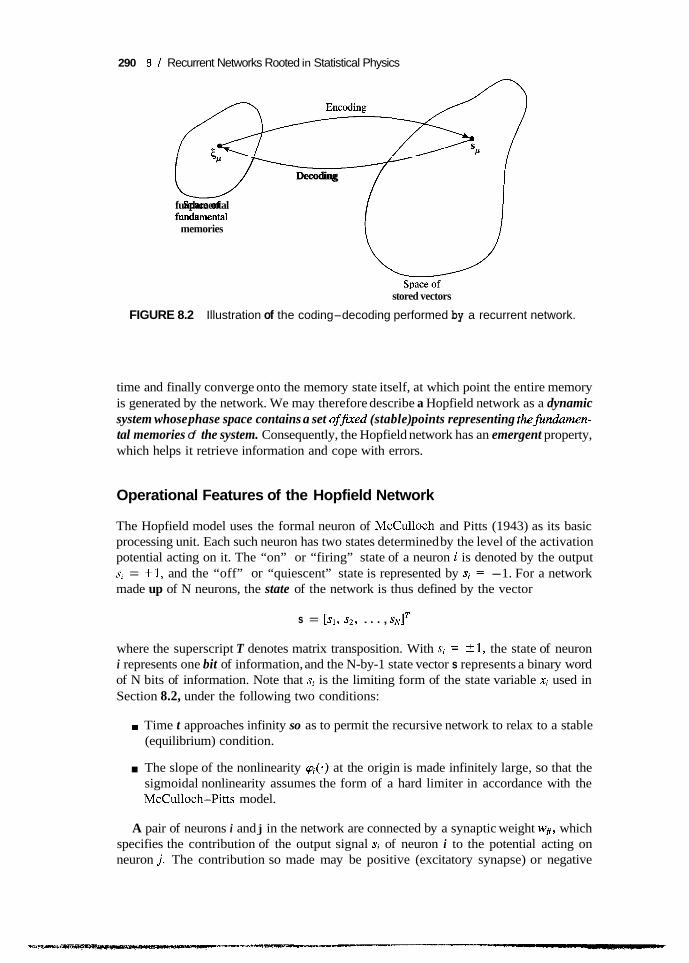
(inhibitory synapse). The net potential u, acting on neuron j is the sum of all postsynaptic potentials delivered to it, as illustrated in the signal-flow graph of Fig. 8.3. Specifically, we may write
where 4 is a fixed threshold applied externally to neuron j . Hence, neuron j modifies its state sj according to the deterministic rule
f l ifu,>O
-1 ifuj<O s j = {
This relation may be rewritten in the compact form
sj = sgn[u,] (8.6)
where sgn is the signum function, defined graphically in Fig. 8.4. What if uj is exactly zero? The action taken here can be quite arbitrary. For example, we may set sj = 21 if uj = 0. However, we will use the following convention: If uj is zero, neuron j remains in its previous state, regardless of whether it is on or off. The significance of this assumption is that the resulting flow diagram is symmetrical, as will be demonstrated later.
There are two phases to the operation of the Hopfield network, namely, the storage phase and the retrieval phase, as described here.
1. Storage Phase. Suppose that we wish to store a set of N-dimensional vectors (binary words), denoted by {&Ip = 1, 2, . . . , p}. We call these p vectorsfundamental memories, representing the patterns to be memorized by the network. Let .$,i denote the ith element of the fundamental memory g,, where the class p = 1,2, . . . , p. According to the outer product rule of storage, that is, the generalization of Hebb’s postulate of learning, the synaptic weight from neuron i to neuron j is defined by
(8.7)
The reason for using 1/N as the constant of proportionality is to simplify the mathematical description of information retrieval. Note also that the learning rule of Eq. (8.7) is a “one- shot” computation. In the normal operation of the Hopfield network, we set
wii = 0 for all i (8.8)
FIGURE 8.3 Signal-flow graph of the net activation potential y of neuron j .

292 8 / Recurrent Networks Rooted in Statistical Physics
FIGURE 8.4 The signum function.
which means that the neurons have no self-feedback. Let W denote the N-by-N synaptic weight matrix of the network, with wji as its jith element. We may then combine Eqs. (8.7) and (8.8) into a single equation written in matrix form as follows:
where ~,gE represents the outer product of the vector 6, with itself, and I denotes the identity matrix. From these defining equations of the synaptic weightslweight matrix, we note the following:
w The output of each neuron in the network is fed back to all other neurons.
w There is no self-feedback in the network (i.e., w,, = 0).
w The weight matrix of the network is symmetric in that we have
w,, = w,, (8.10)
that is, the influence of neuron i on neuron j is equal to the influence of neuron j on neuron i . Equivalently, in matrix form we may write
WT' w The first two conditions are illustrated in the Hopfield network of Fig. 8.5 for the case of N = 4; the boxes labeled z-' represent unit delays.
2. Retrieval Phase. During the retrieval phase, an N-dimensional vector x, called a probe, is imposed on the Hopfield network as its state. The probe vector has elements equal to 5 1. Typically, it represents an incomplete or noisy version of a fundamental memory of the network. Information retrieval then proceeds in accordance with a dynamical rule in which each neuron j of the network randomly but at some fixed rate examines the net activation potential u, (including any nonzero threshold e,) applied to it. If, at that instant of time, the potential u, is greater than zero, neuron j will switch its state to + 1, or remain in that state if it is already there. Similarly, if the potential u, is less than zero, neuron j will switch its state to -1, or remain in that state if it is already there. If U, is exactly zero, neuron j is left in its previous state, regardless of whether it is on or off. The state updating from one iteration to the next is therefore deterministic, but the selection

8.3 / The Hopfield Network 293
1 Unitdelays
FIGURE 8.5 Architectural graph of Hopfield network for N = 4 neurons.
of a neuron to perform the updating is done randomly. The asykchronous (serial) updating procedure described here is continued until there are no further changes to report. That is, starting with the probe vector x, the network finally produces a time-invariant state vector y whose individual elements satisfy the condition for stability:
/ N \
y j = sgn c wjjyi - ej), j = 1,2,. . . , N ( - i= 1 (8.11)
or, in matrix form,
y = sgn(Wy - 0) (8.12)
where W is the synaptic weight matrix of the network, and 6 is the externally applied threshold vector. The stability condition described here is also referred to as the alignment condition. The state vector y that satisfies it is called a stable state or fixed point of the phase space of the system. We may therefore make the statement that the Hopfield network will always converge to a stable state when the retrieval operation is performed asynchronously.
The Little model (Little and Shaw, 1975; Little, 1974) uses the same synaptic weights as the Hopfield model. However, they differ from each other in that the Hopfield model uses asynchronous (serial) dynamics, whereas the Little model uses synchronous (parallel) dynamics. Accordingly, they exhibit different convergence properties (Bruck, 1990; Goles and Martinez, 1990): The Hopfield network will always converge to a stable state, whereas the Little model will always converge to a stable state or a limit cycle of length at most 2. By such a “limit cycle” we mean that the cycles in the state space of the network are of a length less than or equal to 2.

294 8 / Recurrent Networks Rooted in Statistical Physics
EXAMPLE 1
To illustrate the emergent behavior of the Hopfield model, consider the network of Fig. 8.6a, which consists of three neurons. The weight matrix of the network is
0 -2 +2 ”--[;; 3 1 -1 41
which is legitimate, since it satisfies the conditions of Eqs. (8.8) and (8.10). The threshold applied to each neuron is assumed to be zero. With three neurons in the network, there are 23 = 8 possible states to consider. Of these 8 states, only the two states (1,-1,l) and (-l,l,-1) are stable; the remaining six states are all unstable. We say that these two particular states are stable, because they both satisfy the alignment condition of Eq. (8.12). For the state vector (1,-1,l) we have
Hard-limiting this result yields
Similarly, for the state vector (- l , l , - 1) we have
which, after hard limiting, yields
Hence, both of these state vectors satisfy the alignment condition. Moreover, following the asynchronous updating procedure described earlier, we get
the flow described in Fig. 8.6b. This flow map exhibits symmetry with respect to the two stable states of the network, which is intuitively satisfying. This symmetry is the result of leaving a neuron in its previous state if the net potential acting on it is exactly zero.
Figure 8.6b also shows that if the network of Fig. 8.6a is in the initial state (l , l , l) , (-1,-l,l), or (1,-1,-l), it will converge onto the stable state (1,-1,l) after one iteration. If the initial state is (-1,-1,-l), (-l,l,l), or (l,l,-l), it will converge onto the second stable state (- 1,1, - l), also after one iteration.
The network therefore has two fundamental memories ( 1, - 1,l) and ( - 1 , 1 , - 1 ),
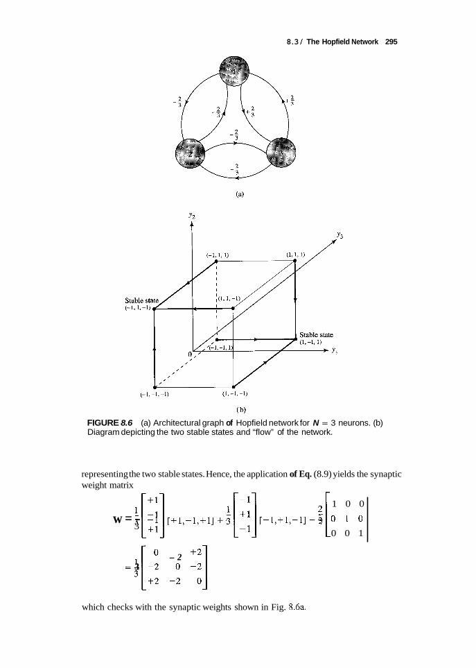
8.3 I The Hopfield Network 295
(-l,-l,-l) (1, -1, -1)
( b)
FIGURE 8.6 (a) Architectural graph of Hopfield network for N = 3 neurons. (b) Diagram depicting the two stable states and “flow” of the network.
representing the two stable states. Hence, the application of Eq. (8.9) yields the synaptic weight matrix
1 0 0
w = - -1 [+1,-1,+1]+- +1 [-1,+1,-11-- 0 1 0 0 0 1
3 f::] :[::I :[ - 2 + 2 -[;a 3 1 -; -;I
which checks with the synaptic weights shown in Fig. 8.6a.

296 8 / Recurrent Networks Rooted in Statistical Physics
The error-correcting capability of the Hopfield network is readily seen by examining
1. If the probe vector x applied to the network equals (-1,-l,l), (l , l , l) , or (1, - 1, - l) , the resulting output is the fundamental memory (1, - 1,l). Each of these values of the probe represents a single error, compared to the stored pattern.
2. If the probe vector x equals (l,l,-1), (-1,-l,--l), or (-l,l,l), the resulting network output is the fundamental memory (- l , l , - 1). Here again, each of these values of the probe represents a single error, compared to the stored pattern.
the flow map of Fig. 8.6b:
Summary of the Hopfield Model
The operational procedure for the Hopfield network may now be summarized as follows:
1. Storage (Learning). Let el, &, . . . , Q denote a known set of N-dimensional memo- ries. Construct the network by using the outer product rule (Le., Hebb's postulate of learning) to compute the synaptic weights of the network as
j = i
where wji is the synaptic weight from neuron i to neuron j . The elements of the vector E, equal 5 1. Once they are computed, the synaptic weights are kept fixed.
2. Initialization. Let x denote an unknown N-dimensional input vector (probe) presented to the network. The algorithm is initialized by setting
sj(0) = xj, j = 1, . . . , N
where sj(0) is the state of neuron j at time n = 0, and xj is the jth element of the probe vector x.
3. Iteration untiE Convergence. Update the elements of state vector s(n) asynchronously (i.e., randomly and one at a time) according to the rule
Repeat the iteration until the state vector s remains unchanged.
step 3. The resulting output vector y of the network is 4. Outputting. Let Sfixed denote the fixed point (stable state) computed at the end of
Y = %?xed
8.4 Computer Experiment I In this section we use a computer experiment to illustrate the behavior of the Hopfield ~
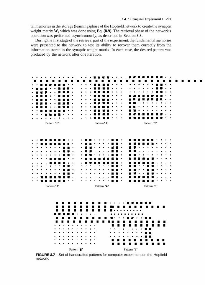
network as a content-addressable memory. The network used in the experiment consists of N = 120 neurons, and therefore N 2 - N = 12,280 synaptic weights. It was trained to retrieve the eight digitlike black-and-white patterns shown in Fig. 8.7, with each pattern containing 120 pixels (picture elements) and designed specially to produce good perfor- mance (Lippmann, 1987). The inputs applied to the network assume the value +1 for black pixels and - 1 for white pixels. The eight patterns of Fig. 8.7 were used as fundamen-
8.4 / Computer Experiment I 297
tal memories in the storage (learning) phase of the Hopfield network to create the synaptic weight matrix W, which was done using Eq. (8.9). The retrieval phase of the network's operation was performed asynchronously, as described in Section 8.3.
During the first stage of the retrieval part of the experiment, the fundamental memories were presented to the network to test its ability to recover them correctly from the information stored in the synaptic weight matrix. In each case, the desired pattern was produced by the network after one iteration.
.............................. .............................. .............................. .............................. .............................. o m ~ m - e m w m - e o - m m . m . o * m r n m m m m m m e - .............................. .............................. .............................. .............................. .............................. ..............................
Pattern "0" Pattern " 1 " Pattern "2"
.............................. .............................. . . . . . . . . . . . . . . . . . . . . . . . . . . . . . . . . . . . . . . . . . . . . . . . . . . . . . . . . . . . . . . . . . . . . . . . . . . . . . . . . . . . . . . . . . . ..............................
. . . . . . . . . . . . . . . . . . . . . . . . . . . . . . . . . . . . . . . . . . . . . . . . . . . . . . . . . . . . . . . . . . . . . . . . . . . . . . . . . . . . . . . . . . .............................. .............................. Pattern "3" Pattern "4" Pattern "6"
o * * o w . m m . e o m m m m m m m m - m m r n m m ~ . e ~ *
.......... .......... .......... .......... .......... m . . m . ~ o o - *
. . . . . . . . . . . . . . . . . . . . . . . . . . . . . . . . . . . . . . . . . . . . . . . . . .
. . e . . * . e . .
~ - ~ * r n ~ m w m r n .......... .......... .......... .......... .......... .......... . . * . 0 . . D . .
'*'e"".. . . . . . . . . . . .......... .......... Pattern "I" Pattern "9"
FIGURE 8.7 Set of handcrafted patterns for computer experiment on the Hopfield network.
298 8 / Recurrent Networks Rooted in Statistical Physics
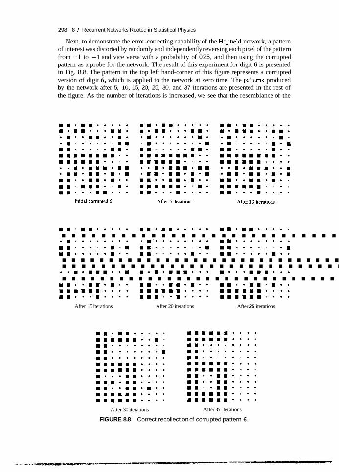
Next, to demonstrate the error-correcting capability of the Hopfield network, a pattern of interest was distorted by randomly and independently reversing each pixel of the pattern from + 1 to -1 and vice versa with a probability of 0.25, and then using the corrupted pattern as a probe for the network. The result of this experiment for digit 6 is presented in Fig. 8.8. The pattern in the top left hand-corner of this figure represents a corrupted version of digit 6, which is applied to the network at zero time. The palterns produced by the network after 5, 10, 15, 20, 25, 30, and 37 iterations are presented in the rest of the figure. As the number of iterations is increased, we see that the resemblance of the
.............................. .............................. . . . . . . . . . . . . . . . . . . . . . . . . . . . . . . . . . . . . . . . . . . . . . . . . . . . . . . . . . . . . . . . . . . . . . . . . . . . . . . . . . . . . . . . . . . .............................. .............................. .............................. ..............................
. . * O M . * . * * . B e * . . * . " W . * e . . o W o -
.............................. After 15 iterations After 20 iterations After 25 iterations
~ ~ . . m r n o e o * m m m m m . . o o e m m ~ . m m o o ~ e
After 30 iterations After 37 iterations
FIGURE 8.8 Correct recollection of corrupted pattern 6.
8.4 / Computer Experiment I 299 . 8
Initial corrupted 2 After 6 iterations After 12 iterations
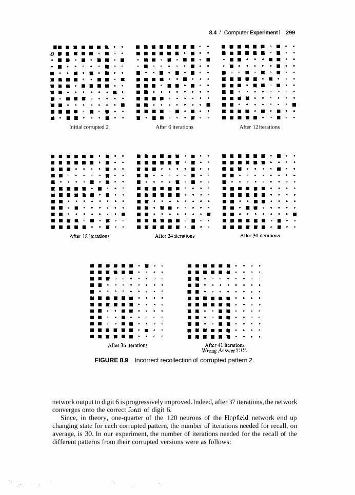
FIGURE 8.9 Incorrect recollection of corrupted pattern 2.
network output to digit 6 is progressively improved. Indeed, after 37 iterations, the network converges onto the correct form of digit 6.
Since, in theory, one-quarter of the 120 neurons of the Hopfield network end up changing state for each corrupted pattern, the number of iterations needed for recall, on average, is 30. In our experiment, the number of iterations needed for the recall of the different patterns from their corrupted versions were as follows:

300 8 / Recurrent Networks Rooted in Statistical Physics
Number of patterns Pattern needed for recall
0 1 2 3 4 6 “0”
9
34 32 26 37 25 37 32 26
The average number of iterations needed for recall, averaged over the 8 patterns, was thus about 31, which shows that the Hopfield network behaved as expected.
However, some problems inherent to the Hopfield network were encountered in the course of the experiment. The first of these problems is that the network is presented with a corrupted version of a fundamental memory, and the network then proceeds to converge onto the wrong fundamental memory. This is illustrated in Fig. 8.9, where the network is presented with a corrupted pattern “2,” but after 41 iterations it converges to the fundamental memory “6.”
The second problem encountered with the Hopfield network is less serious. At times, the network would converge to a pattern that was closer to the desired fundamental memory than to any other, but which still had approximately 5 percent of the neurons of the network assigned to incorrect states. This phenomenon, illustrated in Fig. 8.10 pertaining to digit 9, may be the result of a spurious attractor.
8.5 Energy Function Consider a Hopfield network with symmetric synaptic weights wji = wij and wii = 0. Let si denote the state of neuron i, where i = 1, 2, . . . , N . The energyfunction of the discrete- time version of the Hopfield network considered here is defined by (assuming that the externally applied threshold ej is zero for all j)
(8.13)
The energy change AE due to a change Asj in the state of neuron j is given by
N
AE = - Asj wjjsi (8.14) i = 1 i#j
Thus the action of the algorithm, responsible for changes in the network state during the information retrieval, causes the energy function E to be a monotonically decreasing function of the network state { s j l j = 1, 2, . . . , N } . State changes will continue until a local minimum of the energy landscape is reached, at which point the network stops. The energy landscape describes the dependence of the energy function E on the network state for a specified set of synaptic weights.
The local minima of the energy landscape correspond to the attractors of the phase space, which are the nominally assigned memories of the network. To guarantee the emergence of associative memory, two conditions must be satisfied:

8.5 I Energy Function 301
.............................. ~ r n ~ ~ m m m m m m 0 m o o m . m m r n m ~ . ~ o . . m r n . m .............................. . . . . . . . . . . . . . . . . . . . . . . . . . . . . . . .............................. .... . . . . . . . . . . . . . . . . . . . . . . . . . . .............................. . . . . . . . . . . . . . . . . . . . . . . . . . . . . . . .............................. e o e c . . a o e . . e e e o . o e o D . - o e s . o e * . .
m ~ ~ ~ ~ ~ w m r n r n m ~ ~ ~ ~ w m ~ m r n r n o 0 - m m m . m ~
o m a o m . . r n r n m ~ . o ~ . . m m r n m 0 w ~ o r n m . m m ~
After 12 iterations After 16 iterations After 20 iterations
.......... .......... e o o o . e o 0 . . .......... o * * - m m 4 m m m ~ o ~ * . . m w . r n .......... ..... . . . . . .......... . . . . . . . . . . .......... ..........
After 24 iterations
.......... .......... .......... .......... .......... .......... .......... ... . . . . . . . . . . . . . . . . . . . . . . . . . . . .......... .......... After 28 iterations
Wrong answer ! ! ! ! ! ! !
FIGURE 8.10 Illustration of another aspect of the recollection phenomenon exhibited by the Hopfield network.
The fundamental patterns memorized by the network are all stable. rn The stable patterns have a sizeable basin of attraction (region of influence).
Suppose that the retrieval algorithm is initiated with a probe (i.e., unknown input pattern), representing a starting point in the energy landscape. Then, as the algorithm iterates its way to a solution, the starting point moves through the energy landscape toward a local minimum. When the local minimum is actually reached, the algorithm stays there, because everywhere else in the close vicinity is an uphill climb. The solution produced

302 8 I Recurrent Networks Rooted in Statistical Physics
by the algorithm is represented by the network state at that particular local minimum of the energy landscape.
EXAMPLE 2
Consider again the Hopfield network of Fig. 8.6a. Substituting the synaptic weights of the network in Eq. (8.13) yields the energy function
Table 8.1 shows the values of E calculated for all the eight possible states of the network. This table confirms that the energy function of the network attains its minimum values at the stable states of the network. In the last column of this table we have also included the change AE in the energy function due a change in the state of a single neuron in the network. The reader is invited to check the latter set of results using Eq. (8.14).
Spurious States
When a Hopfield network is used to store K patterns by means of the Hebb prescription of Eq. (8.7) for the synaptic weights, the network is usually found to have spurious uttructors, also referred to as spurious states (Hertz et al., 1991; Amit, 1989). Spurious states represent stable states of the network that are different from the fundamental memories of the network. How do spurious states arise?
First of all, we note that the energy function E is symmetric in the sense that its value remains unchanged if the states of the neurons are reversed (i.e., the state si is replaced by -si for all i). Accordingly, if the fundamental memory ge corresponds to a particular local minimum of the energy landscape, that same local minimum also corresponds to -6,. This is illustrated by the two stable states (-l,+l,--1) and (+l , - l ,+ l ) of the Hopfield network of Fig. 8.6 that was considered in Examples 1 and 2. This sign reversal need not pose a problem in the retrieval of stored information if it is agreed to reverse all the remaining bits of a retrieval pattern if it is found that a particular bit designated as the “sign” bit is - 1 instead of + 1.
Second, there is an attractor for every mixture of the stored patterns (Amit, 1989). A mixture state corresponds to a linear combination of an odd number of patterns. As a
TABLE 8.1 Energy Function of the Hopfield Network of Fig. 8.6a
Network State Energy Function,
S1 s 2 s3 E A E ~
- 1 + 1 -1 + I -1 + I - 1 +1
- 1 -1 f l + 1 - 1 -1 + I + l
- 1 - 1 - 1 -1 + l +1 +1 +l
213 213 0 - 2 - 813 213 813 213 0 - 2 - 813 213 813 213 0

8.6 / Error Performance of the Hopfield Network 303
simple example, consider the network state
si = sgn(&;,i + 6 , i + 53.i) (8.15)
This is a 3-mixture spurious state. It is a state formed out of three random patterns gl, g2, and g3 by a majority rule. The stability condition of Eq. (8.1 1) is indeed satisfied by the 3-mixture state of Eq. (8.15) for a large network (Amit, 1989).
Third, for a large number p of fundamental memories, the energy landscape has local minima that are not correlated with any of these memories embedded in the network. Such spurious states are sometimes referred to as spin-glass states, by analogy with spin- glass models of statistical mechanics; the idea of spin-glass models is discussed in Sections 8.7 and 8.8.
It is of interest to note that the absence of self-feedback, as described in Eq. (8.8), has a beneficial effect insofar as spurious states are concerned. Specifically, if we were to set wii # 0 for all i , additional stable spurious states might be produced in the neighborhood of a desired attractor (Kanter and Sompolinsky, 1987).
8.6 Error Performance of the Hopfield Network Unfortunately, the fundamental memories of a Hopfield network are not always stable. Moreover, spurious states representing other stable states that are different from the fundamental memories can arise. These two phenomena, the probable instability of funda- mental memories and the possible existence of spurious states, tend to decrease the efficiency of a Hopfield network as a content-addressable memory. In this section we use probabilistic considerations to explore the first of these two phenomena.
The summation in Eq. (8.7), defining the synaptic weights wji from neuron i to neuron j , is taken over all the fundamental memories. This equation is reproduced here for convenience of presentation:
Let a probe denoted by the threshold 0, applied neuron is
the vector x be presented to the network. Then, assuming that to neuronj is zero, we find that the potential vj acting on this
(8.16)
where, for the purpose of generality, the use of self-feedback (Le., wii f 0) is permitted. Consider the special case when the probe x equals one of the fundamental memories stored in the network; that is, x = g,,. We may then rewrite Eq. (8.16) as
(8.17)

304 8 / Recurrent Networks Rooted in Statistical Physics
The first term on the right-hand side of Eq. (8.17) is simply the jth element of the fundamental memory gu; now we can see why the scaling factor 1/N was introduced in the definition of the synaptic weight wji in Eq. (8.7). This term may therefore be viewed as the desired “signal” component. The second term on the right-hand side of Eq. (8.17) is the result of “crosstalk” between the elements of the fundamental memory e,, under test and those of some other fundamental memory i&. This second term may therefore be viewed as the “noise” component of vj. We therefore have a situation similar to the classical ‘ ‘signal-in-noise detection problem” in communication theory (Haykin, 1983).
We assume that the fundamental memories are random, being generated as a sequence of pN Bernoulli trials. The noise term of Eq. (8.17) then consists of a sum of N ( p - 1) independent random variables, taking on values 21 divided by N. This is a situation where the central limit theorem of probability theory applies. The central limit theorem states (Feller, 1968):
Let {Xk} be a sequence of mutually independent random variables with a common distribution. Suppose that X , has mean p and variance u2, and let Y = X I + X2 + . . + X,. Then, as n approaches injnity, the probability distribution of the sum random variable Y approaches a Gaussian distribution.
Hence, applying the central limit theorem to the noise term in Eq. (8.17), we find that the noise is asymptotically Gaussian distributed. Each of the N ( p - 1) random variables constituting the noise term in Eq. (8.17) has a mean of zero and a variance of 1/N2. It follows, therefore, that the statistics of the Gaussian distribution are
Zero mean
Variance equal to ( p - l) /N, which is N ( p - 1) times 1/N2
The signal component &,j has a value of + 1 or - 1 with equal probability, and therefore a mean of zero and variance of unity. The signal-to-noise ratio is thus defined by
variance of signal = variance of noise
- _ - for large p P
(8.18)
The components of the fundamental memory E,, will be stable if, and only if, the signal- to-noise ratio p is high. Now, the number p of fundamental memories provides a direct measure of the storage capacity of the network. Therefore, it follows from Eq. (8.18) that so long as the storage capacity of the network is not overloaded-that is, the number p of fundamental memories is small compared to the number N of neurons in the network- the fundamental memories are stable in a probabilistic sense.
Storage Capacity of the Hopfield Network
Let the jth bit of the probe x = eu be a “1,” that is, &,j = +I. Then the conditional probability of bit error is defined by the shaded area shown in Fig. 8.1 1. The rest of the

8.6 I Error Performance of the Hopfield Network 305
0. 0 t”,j=l J
FIGURE 8.1 1 the net activation potential y of neuron j .
Conditional probability of bit error, assuming a Gaussian distribution for
area under this curve is the conditional probability that bit j of the probe is retrieved correctly. Using the well-known formula for a Gaussian distribution, this latter conditional probability is given by
(8.19) Prob(uj > 01 &,j = + 1) = -I,” 1 exp (- 7) (Vi- P ) ~ duj v5-u With &,j set to fl, and the mean of the noise term in Eq. (8.17) equal to zero, it follows that the mean of the random variable vj is
p = 1
and its variance is
From the definition of the errorfinction commonly used in calculations involving the Gaussian distribution, we have
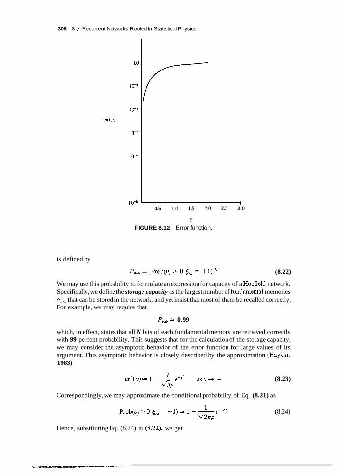
2 erf( y ) = - e-2 dz fi (8.20)
where y is a variable defining the upper limit of integration. A plot of erf( y ) versus y is presented in Fig. 8.12. Note that as y approaches infinity, the error function erf(y) approaches unity.
We may now simplify the expression for the conditional probability of correctly retrieving the jth bit of the fundamental memory by rewriting Eq. (8.19) in terms of the error function as follows:
- Prob(vj > O[&,j = +1) = (8.21)
where p is the signal-to-noise ratio defined in Eq. (8.18). Each fundamental memory consists of n bits. Also, the fundamental memories are
usually equiprobable. It follows therefore that the average probability of stable patterns
306 8 / Recurrent Networks Rooted in Statistical Physics
1 .a
10-1
10-2
erfcy)
10-~
10-4
10-6 I 0.5 1.0 1.5 2.0 2.5 3.0
Y
FIGURE 8.12 Error function.
is defined by
Pstab = [Prob(uj > O1&j = +1)IN (8.22)
We may use this probability to formulate an expression for capacity of a Hopfield network. Specifically, we define the storage capacity as the largest number of fundamental memories pmax that can be stored in the network, and yet insist that most of them be recalled correctly. For example, we may require that
Psbb E 0.99
which, in effect, states that all N bits of each fundamental memory are retrieved correctly with 99 percent probability. This suggests that for the calculation of the storage capacity, we may consider the asymptotic behavior of the error function for large values of its argument. This asymptotic behavior is closely described by the approximation (Haykin, 1983)
(8.23) 1 erf(y) 1 - -e-Y* asy+ 00
G Y Correspondingly, we may approximate the conditional probability of Eq. (8.21) as
(8.24)
Hence, substituting Eq. (8.24) in (8.22), we get

8.6 / Error Performance of the Hopfield Network 307
(8.25)
where, in the second line, we have used the approximation to the binomial expansion. The second term in Eq. (8.25) must be negligible compared to the unity term as the
network N is made infinitely large in order to ensure that the average probability of stable patterns Psmb is close to unity. We note that the second term in E$. (8.24) is the average probability that a bit in a fundamental memory will be unstable. Now, it is not enough to require the probability for one unstable bit be small, but rather it must be small compared with 1IN. This requirement is satisfied provided that we choose
1 1 - e - P / 2 < - N
or, equivalently,
1 2
p>2lnN+- ln(2rp)
To ensure the stability of most of the fundamental memories, we must therefore choose the signal-to-noise ratio such that its minimum value satisfies the condition (Amit, 1989)
pmin = 2 In N (8.26)
We may then rewrite Eq. (8.25) simply as
1 2 G N
P s m b = 1 - (8.27)
Equation (8.27) shows that, in the limit as the number of neurons N approaches infinity, the probability that there will be an unstable bit in a state of the Hopfield network corresponding to any of the fundamental memories approaches zero. This result, however, is subject to the requirement that the signal-to-noise ratio p is not permitted to drop below the minimum value pmin of Eq. (8.26) or, equivalently, that the number of fundamental memories p does not exceed a critical value p- . In light of this requirement, we may use the definition of p given in the last line of Eq. (8.18) to write
N 21nN
- -- (8.28)
Equation (8.28) defines the storage capacity of a Hopfield network on the basis that most of the fundamental memories are recalled pevectly.
In our definition of the storage capacity, we could be even more stringent by requiring that aZZ the fundamental memories be recalled perfectly. Such a definition requires that all pN bits of the fundamental memories are retrieved correctly with a probability of 99 percent, say. Using this definition, it can be shown that the maximum number of fundamen- tal memories is given by (Amit, 1989)
N Pmax = - 41nN (8.29)

308 8 / Recurrent Networks Rooted in Statistical Physics
The important point to note is that whether we use the definition of Eq. (8.28) or the more stringent one of Eq. (8.29) for the storage capacity of a Hopfield network, the asymptotic storage capacity of the network has to be maintained small for the fundamental memories to be recoverable. This is indeed a major limitation of the Hopfield network.
How to Increase the Storage Capacity
One way of suppressing the adverse effects of correlated patterns in the Hopfield network is to modify the outer product rule of learning by makmg it nonlocal in character. In particular, the synaptic weight wji is redefined by (Personnaz et al., 1985)
(8.30)
where (C-’),, is the pvth element of the inverse matrix C-’. The pvth element of the overlap matrix C is defined by
(8.31)
Dynamics of the network so defined is not governed by the energy function of Eq. (8.13) because of the presence of self-coupling terms. The self-coupling severely restricts the size of the basins of attraction of the fundamental memories, especially for largep. Kanter and Sompolinsky (1987) have introduced a modification of the model of Personnaz et al. by eliminating the self-coupling terms from the dynamics. The resulting network has the ability to retrieve perfectly any p linearly independent patterns for all p < N , where N is the number of neurons. The fact that the patterns memorized by the network can be retrieved without errors and that correlated patterns can also be stored is a good advantage. The price paid for this improvement is that the learning rule is nonlocal, which makes the model unattractive from a biological viewpoint.
8.7 Isomorphism Between a Hopfield Network and a Spin-Glass Model
A Hopfield model consists of a large assembly of identical neurons, each characterized by an internal state (Le., firing rate), and interconnected by synapses of varying weights in accordance with a dynamic rule. Such a model is reminiscent of some simple models of magnetic materials encountered in statistical mechanics.
Consider a solid consisting of N identical atoms arranged in a regular lattice. Each atom has a net electronic spin and associated magnetic moment. In a well-known example in statistical mechanics referred to as the Ising-spin model, the spin uj of each atom j can only take on the value ? 1. In addition, each atom is assumed to interact with neighboring atoms. The predominant iteration is usually the so-called exchange iteration, which is a quantum mechanical effect. If the spin-spin interactions extend over large distances and take on random values, we speak of a spin-glass model.
Much research in condensed matter physics has been directed at “frustrated” systems, in which atoms are not all alike. The term “frustration” refers to the feature that interactions favoring different and incompatible kinds of ordering may be simultaneously present. The magnetic alloys known as ‘ ‘spin glasses,” which exhibit competition between ferromag- netic and antiferromagnetic spin ordering, are the best example of frustrated systems. These systems stand in the same relation to conventional magnets as glasses do to crystals-hence

8.8 / Stochastic Neurons 309
the name “spin glass” (Kirkpatrick et al., 1983). The ferromagnetic use corresponds to the case for whch all the wjj are positive. The antiferromagnetic use, on the other hand, corresponds to the case where there is a regular change of sign between neighboring atoms. If the signs and absolute values of wij are randomly distributed, the material is called a spin glass.
The dynamics of the spin-glass model is viewed in a phase space that is spanned by the degrees of freedom and the associated moments. The system is governed by a Hamiltonian through the usual equations of motion. The internal states of the system are represented by the spin variables q, j = 1,2, . . . , N . For the system to evolve toward an equilibrium state, we assume the existence of an unspecified mechanism that permits the spins to flip up or down, according to the following rules:
1. Every atom j in the model is associated with a quantity called the molecularjeld hj. 2. The molecular field hj is a linear combination of the internal states q of the sur-
rounding spins:
hj = Jiui I
(8.32)
where the coefficients Jj are called the exchange couplings. 3. The internal state q eventually flips so as to satisfy the alignment condition:
h jq > 0 (8.33)
The Hamiltonian H representing the interaction energy between the spins of the system is defined by
1 2 ; j
= - - J..g.(+. 11 I 1
(8.34)
where the factor 4 is introduced because the interaction between the same two spins is counted twice in performing the double summation. When the exchange couplings are symmetric, that is,
J.. I‘ = J . . 11 (8.35)
but they have a random character, the system is known to have many locally stable states. Comparing the equations that characterize the spin-glass model with those of the
Hopfield model, we see immediately that there is indeed an isomorphism between these two models. The details of this isomorphism are presented in Table 8.2.
Physicists have devoted a great deal of work to the statistical mechanics of spin-glass models, which means that the formal methods and concepts of statistical mechanics are natural tools for the study of not only the Hopfield network but also other related neural networks (Peretto, 1984). The most significant results have been obtained with fully connected spin networks (Kirkpatrick and Sherrington, 1978).
8.8 Stochastic Neurons Up to now, we have focused our attention on the “noiseless” dynamics of the Hopfield model-noiseless in the sense that there is no noise present in the synaptic transmission of signals. In reality, however, synaptic transmission in a nervous system is a noisy

310 8 I Recurrent Networks Rooted in Statistical Physics
TABLE 8.2 Dictionary Describing Isomorphism Between the Hopfield and Spin-Glass Models
Hopfield Model Spin-Glass Model
Neuron i Atom i Neuron state s, = +1 Synaptic weights, wJl Net activation potential, u,
Spin ut = -tl Exchange couplings, Jt Molecular field, h,
Excitatory synapse, w,, > 0 Inhibitory synapse, w,, < 0
4, > 0 Jj, < 0
Energy function, E Hamiltonian, H
process brought on by random fluctuations from the release of neurotransmitters, and other probabilistic causes. The important question, of course, is how to account for the effects of synaptic noise in a neural network in a mathematically tractable manner. The traditional method for doing so in the neural network literature is to introduce aprobabilistic mechanism in the $ring of neurons and, in a loose sense, to represent the effects of synaptic noise by thermal jluctuations. Specifically, a neuron j decides to fire according to the value of the net potential uj acting on it with the probability ofjring being defined by P(vj) . We thus replace the deterministic rule of Eq. (8.5) for the state sj of neuron j by the probabilistic rule
+ 1 with probability P(uj)
- 1 sj= {
with probability 1 - P(uj) (8.36)
If the net potential probability i.
uj acting on neuron j is exactly zero, we set sj = 2 1 each with
For the function P(v) to qualify as a probability, it must satisfy the limiting values
P(u) = 0 as u -+ -a
and
P(v ) = 1 as u -+ + w
Moreover, between these two limits, the function P(u) must increase monotonically with u. A standard choice for P(v) is the sigmoid-shaped function (Little, 1974):
1 ‘(’) = 1 + exp(-2ulT)
(8.37)
where T is a pseudotemperature that is used to control the noise level and therefore the uncertainty in the firing of a neuron. It is important to realize, however, that Tis not the physical temperature of a neural network, be that a biological or an artificial network. Rather, as already stated, we should think of T as a parameter that controls the thermal fluctuations representing the effects of synaptic noise. For brevity, however, we will refer to Tin the context of neural networks simply as “temperature” hereafter.
When T -+ 0, which corresponds to the noiseless limit, the width of the threshold region shrinks to zero. Under this condition, the probabilistic firing rule of Eq. (8.36) reduces to the deterministic rule of Eq. (8.5). Figure 8.13 displays the probability P(u) that a neuron fires, which is plotted as a function of the net potential u acting on the neuron for two different values of the temperature T. The continuous curve represents a plot of Eq. (8.36) for some temperature T greater than zero, whereas the curve shown in

8.9 / Phase Diagram of the Hopfield Network 311
0
FIGURE 8.13 Sigmoid-shaped function for probability of a stochastic neuron firing; heavy solid curve corresponds to the operation of the McCulloch-Pitts neuron.
heavy solid lines represents the limiting case of T = 0. Note that although the continuous curve in Fig. 8.13 has the same sigmoidal shape as the activation function of a nonlinear neuron in multilayer perceptrons, it has an entirely different meaning. The sigmoid function plotted in Fig. 8.13 represents a probabilistic threshold response, whereas the sigmoidal activation function in a multilayer perceptron represents a deterministic input-output relation.
It is also of interest to note that the probabilistic rule of Eq. (8.36) is consistent with the way in which the effect of thermal fluctuations in a spin-glass model is described mathematically. Indeed, the use of the probabilistic rule for the firing of a neuron as described here makes the analogy between the Hopfield model in neural networks and the spin-glass model in statistical mechanics all the more complete and fruitful.
8.9 Phase Diagram of the Hopfield Network, and Related Properties
The striking similarity between the behavior of the Hopfield network and that of the spin- glass model has led to the discovery of an important property of the Hopfield network: It is solvable exactly. Specifically, starting with the energy function (i.e., Hamiltonian) of the Hopfield network and the generalized Hebb rule for the synaptic weights of the network, and assuming that the number N of neurons in the network is large (i.e., invoking the thermodynamical limit N 4 w), Amit and co-workers’ used the formal methods and concepts of statistical mechanics to derive the mean-jield equations for associative recall in a stochastic Hopfield network (Le., one that uses stochastic neurons). The mathematics involved in the derivation is rigorous and difficult to plough through, and unfortunately beyond the scope of this book. We will therefore content ourselves by describing highlights of the theory.
’ The derivation of the mean-field equations for the Hopfield network was first reported in a remarkable series of papers (Amit et al., 1985a, 1985b; 1987a, 1987b), which were followed by a book (Amit, 1989). For a condensed treatment of the subject, see chaps. 16 and 17 of the book by Muller and Reinhardt, (1990), and chap. 1 by van Hemmen and Kuhn in the book edited by Domany et al. (1991).
The term “mean field” in mean-field equations comes from statistical physics. It refers to the mean value of the molecular field associated with each atom in a spin-glass model.

312 8 / Recurrent Networks Rooted in Statistical Physics
The mean-field equations involve the following variables (among others):
The mean (average) values of the states sj of neurons in the network
(sj), j = 1, 2, . . . , N
A set of auxiliary variables, m,, characterizing the mean overlap of (s j ) with the stored pattern &,j for j = 1, 2, . . . , N :
. N
v = 1 ,2 , . . (8.38)
where p is the number of memorized patterns (fundamental memories). In other words, m, provides a measure of retrieval quality.
The load parameter or storage ejficiency,
a = - P N (8.39)
which expresses the number of memorized patterns, p , as a fraction of the total number of neurons in the network, N . Note that for a # 0, the numberp of memorized patterns scales proportionately with the number N of neurons, as N 3 UJ. Note also that a is the reciprocal of the signal-to-noise ratio p for large N, see Eq. (8.18).
The temperature T, which provides a measure of how noisy the network dynamics is.
For a complete description of a stochastic Hopfield network required to recall memorized patterns, we have to consider m as a function of both a and T. This evaluation leads to the formulation of the T-a phase diagram, depicted in Fig. 8.14. The phase diagram delineates three main critical lines labeled T,, TM, and T,, across which the Hopfield network changes its qualitative behavior.
The phase boundary between the network functioning as an associative memory and one suffering from total confusion or amnesia is described by the curve labeled TM in
LO( T 0.01 0.02[
T
, I I I I I I I i A A A i "." 0.00 0.05 0.10 0.15
cy cyc = 0.138
FIGURE 8.14 Phase diagram of the Hopfield network. (From E. Domany et ai., 1991, with permission of Springer-Verlag.)
8.9 / Phase Diagram of the Hopfield Network 313
Fig. 8.14. This curve is bounded by the critical load parameter a, = 0.138 on the a axis and the critical temperature T = 1 on the T axis. Directly below TM the retrieval states of the Hopfield network are metastable, with few spin errors. If a < 0.051, we pass the line T,, below which the retrieval states of the network are globally stable, with no spin errors. In the no-recall area above the curve TM in Fig. 8.14, the only stable states are the spin-glass (spurious) states. In the no-recall area, above the line Tg, these spin-glass states “melt”; the resulting solution produced by the network has an average value of zero. Near a, = 0.138 there is another critical line TR, below which the replica symmetry of the retrieval states breaks down. What this implies is that within the retrieval states, a fraction of the spins (neurons) freeze in a spin-glass fashion. As the inset of the phase diagram in Fig. 8.14 shows, this instability is restricted to a fairly small region and therefore has a very small impact on the quantities that are relevant to retrieval.
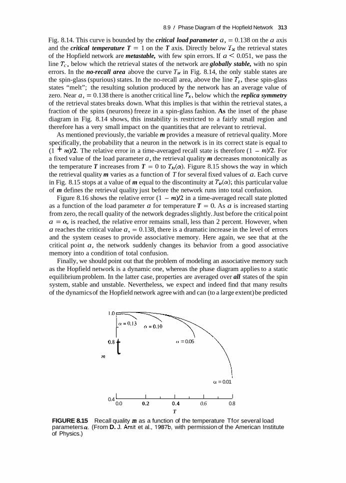
As mentioned previously, the variable m provides a measure of retrieval quality. More specifically, the probability that a neuron in the network is in its correct state is equal to (1 + m)/2. The relative error in a time-averaged recall state is therefore (1 - m)/2. For a fixed value of the load parameter a, the retrieval quality m decreases monotonically as the temperature T increases from T = 0 to TM(a). Figure 8.15 shows the way in which the retrieval quality m varies as a function of T for several fixed values of a. Each curve in Fig. 8.15 stops at a value of m equal to the discontinuity at TM(a); this particular value of m defines the retrieval quality just before the network runs into total confusion.
Figure 8.16 shows the relative error (1 - m)/2 in a time-averaged recall state plotted as a function of the load parameter a for temperature T = 0. As a is increased starting from zero, the recall quality of the network degrades slightly. Just before the critical point a = a, is reached, the relative error remains small, less than 2 percent. However, when a reaches the critical value a, = 0.138, there is a dramatic increase in the level of errors and the system ceases to provide associative memory. Here again, we see that at the critical point a, the network suddenly changes its behavior from a good associative memory into a condition of total confusion.
Finally, we should point out that the problem of modeling an associative memory such as the Hopfield network is a dynamic one, whereas the phase diagram applies to a static equilibrium problem. In the latter case, properties are averaged over all states of the spin system, stable and unstable. Nevertheless, we expect and indeed find that many results of the dynamics of the Hopfield network agree with and can (to a large extent) be predicted
t rn
\ a = 0.05
cy = 0.01
0.4 ‘ I I I I I I I 0.0 0.2 0.4 0.6 0.8
T
FIGURE 8.15 Recall quality m as a function of the temperature Tfor several load parameters a. (From D. J. Amit et al., 1987b, with permission of the American Institute of Physics.)

314 8 / Recurrent Networks Rooted in Statistical Physics
(1 - m)/2 1 2.0 c
0.5
0.0 0.05
a, = 0.138 a
FIGURE 8.16 The quality of memory recall of the Hopfield network deteriorates with increasing load parameter a = p/N and breaks down at a = 0.138. (From B. Muller and J. Reinhardt, 1990, with permission of Springer-Verlag.)
from the static equilibrium calculation (Domany, 1988). For instance, the critical load parameter CY, = 0.138 is in agreement with the estimate of Hopfield (1982), where it is reported that (as a result of computer simulations) about 0.15N states can be recalled simultaneously before error becomes severe.
8.1 0 Simulated Annealing Sections 8.3 through 8.9 were concerned strictly with different aspects of the Hopfield network. We now turn our attention to simulated annealing, which is important not only in its own right as a technique for solving combinatorial optimization problems, but also because it provides the basis for the Boltzmann machine to be considered in Section 8.1 1. A discussion of simulated annealing is also considered rather appropriate at this juncture, as it flows quite nicely from the stochastic notions presented in the previous two sections.
In a neural network, the objective is often that of minimizing a cost function defined as the global energy of the network. Ordinarily, the number of neurons contained in the network is very large. Thus, finding the minimum-energy solution of a neural network is not unlike that of finding the low-temperature state of a physical system. However, as mentioned previously, the concept of the temperature of a physical system has no obvious equivalent in a neural network.
Another issue of concern is that deterministic algorithms used for energy minimization suffer from a fundamental weakness of gradient descent procedures: The algorithm may get “stuck” in “local minima” that are not globally optimum. In the case of a Hopfield network used for “noiseless” pattern storage and recognition, this issue is not a problem, because the local energy minima of the network are exploited as a means of storing input patterns. This issue is of particular concern, however, in the case of neural networks required to perform construint-satisfaction tasks. Specifically, when some of the neurons in a neural network are externally forced or “clamped” to some input pattern, we have to find a minimum-energy solution compatible with that particular input pattern. In such a situation, the network must be capable of escaping from local minima so as to reach the configuration that represents the global minimum, given the input pattern of interest.
Both of these issues are addressed in the simulated annealing algorithm, which was originally developed by Kirkpatrick et al. (1983). The basic idea of the algorithm is quite simple:

8.10 / Simulated Annealing 315
When optimizing a very large and complex system (i.e., a system with many degrees of fYeedom), instead of “always” going downhill, try to go downhill “most of the time. ’ ’
Simulated annealing differs from conventional iterative optimization algorithms in two important respects:
The algorithm need not get stuck, since transition out of a local minimum is always possible when the system operates at a nonzero temperature.
Simulated annealing exhibits a divide-and-conquer feature that is adaptive in nature. Specifically, gross features of the final state of the system are seen at higher tempera- tures, while fine details of the state appear at lower temperatures.
The simulated annealing algorithm is based on the analogy between the behavior of a physical system with many degrees of freedom in thermal equilibrium at a series of finite temperatures as encountered in statistical physics and the problem of finding the minimum of a given function depending on many parameters as in combinatorial optimization (Kirkpatrick et al., 1983). In condensed-matter physics, annealing refers to a physical process that proceeds as follows (van Laarhoven and Aarts, 1988):
1. A solid in a heat bath is heated by raising the temperature to a maximum value at which all particles of the solid arrange themselves randomly in the liquid phase.
2. Then the temperature of the heat bath is lowered, permitting all particles to arrange themselves in the low-energy ground state of a corresponding lattice.
It is presumed that the maximum temperature in phase 1 is sufficiently high, and the cooling in phase 2 is carried out sufficiently slowly. However, if the cooling is too rapid- that is, the solid is not allowed enough time to reach thermal equilibrium at each temperature value-the resulting crystal will have many defects, or the substance may form a glass with no crystalline order and only metastable locally optimal structures (Kirkpatrick et al., 1983).
In 1953, Metropolis et al. proposed an algorithm for efficient simulation of the evolution to thermal equilibrium of a solid for a given temperature. The simulated annealing algo- rithm developed by Kirkpatrick et al. (1983) is a variant (with time-dependent temperature) of the Metropolis algorithm.2
Metropolis Algorithm
The Metropolis algorithm, based on Monte Carlo techniques, provides a simple method for simulating the evolution of a physical system in a heat bath (reservoir) to thermal equilibrium. It was introduced in the early days of scientific computation for the efficient simulation of a collection of atoms in equilibrium at a given temperature. In each step of the algorithm, an atom (unit) of a system is subjected to a small random displacement, and the resulting change AE in the energy of the system is computed. If we find that the change AE 5 0, the displacement is accepted, and the new system configuration with the displaced atom is used as the starting point for the next step of the algorithm. If, on the other hand, we find that the change AE > 0, the algorithm proceeds in a probabilistic manner, as described next. The probability that the configuration with the displaced atom
* The Langevin equation (with time-dependent temperature) provides the basis for another global optimization algorithm that was proposed by Grenander (1983), and subsequently analyzed by Gidas (1985). The Langevin equation is described in Appendix D at the end of the book.

316 8 / Recurrent Networks Rooted in Statistical Physics
accepted is given by, except for a scaling factor,
(8.40)
where Tis the temperature. To implement the probabilistic part of the algorithm, we may use a generator of random numbers distributed uniformly in the interval (0,l). Specifically, one such number is selected and compared with the probability P(AE) of Eq. (8.40). If the random number is less than the probability P(AE) , the new configuration with the displaced atom is accepted. Otherwise, the original system configuration is reused for the next step of the algorithm.
Provided that the temperature is lowered in a sufficiently slow manner, the system can reach thermal equilibrium at each temperature. In the Metropolis algorithm, this condition is achieved by having a large number of transitions at each temperature; a transition refers to some combined action that results in the transformation of a system from one state to another. Thus, by repeating the basic steps of the Metropolis algorithm, we effectively simulate the motion of the atoms in a physical system in thermal equilibrium with a heat bath of absolute temperature T. Moreover, the choice of P ( A E ) defined in Eq. (8.40) ensures that thermal equilibrium is characterized by the Boltzmann distribution, just as in statistical mechanics. According to the Boltzmann distribution, described in Appendix C at the end of the book, the probability of a physical system being in a state cy with energy E, at temperature T is given by
Pa = -exp 1 (- $) Z
where Z is the partition @nction, defined by
z = exp (- :) P
(8.41)
(8.42)
where the summation is taken over all states /3 with energy Ep at temperature T. At high values of temperature T, the Boltzmann distribution exhibits a uniform preference for all states, regardless of energy. When the temperature T approaches zero, however, only the states with minimum energy have a nonzero probability of occurrence.
Markov Property of Simulated Annealing
Given a neighborhood structure, we may view the simulated annealing algorithm as an algorithm that continuously tries to transform the current configuration into one of its neighbors. In mathematical terms, such a mechanism is best described by means of a Markov chain (van Laarhoven and Aarts, 1988).
To define what we mean by a Markov chain, consider a probabilistic experiment involving a sequence of trials with possible outcomes {A,, n = 0, 1, 2, . . .}, which is characterized in such a way that the conditional probability of the outcome A, depends only onA,-l and is independent of all previous outcomes. More precisely, let the conditional probability of the event (outcome) A,, given that An-l, . . . , A. have occurred, satisfy the condition
Prob(A,IA,-l, . . . , A,) = Prob(A,IA,-,) (8.43)
A sequence of trials whose outcomes {An, n = 0, 1 , 2, . . .} satisfy this condition is said to be a Markov chain (Feller, 1968; Bharucha-Reid, 1960).

8.10 / Simulated Annealing 317
In the case of simulated annealing, trials correspond to transitions and outcomes correspond to system configurations (states). Since, in simulated annealing, the current state of a system that has experienced a transition depends only on the previous state, it follows that simulated annealing has the Markov property.
A Markov chain is described in terms of a set of one-step transition probabilities pji(n, n - 1). Specifically, pji(n, n - 1) is the conditional probability that the system is in state j after the nth transition, given that it was in state i after the (n - 1)th transition. Let Pj(n) denote the absolute or unconditional probability that the system is in state j after the nth transition. We may then solve for Pj(n) using the recursion
I
(8.44) k
where the summation is over all possible states of the system. If the transition probabilities pjk(iz, n - 1) do not depend on n, the Markov chain is said to be homogeneous.
Finite-Time Approximation
An important property of simulated annealing is that of asymptotic convergence, for which a mathematical proof was first given by Geman and Geman (1984). According to Geman and Geman, we may state the following:
If the temperature Tk employed in executing the kth step of the simulated annealing algorithm satisjies the bound
TO log(1 + k)
Tk 2 (8.45)
for every k, where To is a suficiently large constant (initial temperature) independent of k, then with probability one the system will converge to the minimum energy conjguration.
Stated in another way, the algorithm generates a Markov chain that converges in distribu- tion to a uniform one over the minimal energy configurations. The conditions for asymptotic convergence given here are suficient but not necessary. Similar conditions for asymptotic convergence of the simulated annealing algorithm have been derived by many other authors (Aarts and Korst, 1989).
Unfortunately, the annealing schedule specified by Eq. (8.45) is extremely slow-too slow to be of practical use. In practice, we have to resort to ajinite-time approximation of the asymptotic convergence of the algorithm. The price paid for the approximation is that the algorithm is no longer guaranteed to find a global minimum with probability 1. Nevertheless, the resulting approximate form of the algorithm is capable of producing near-optimum solutions for many practical applications.
To implement a finite-time approximation of the simulated annealing algorithm, we need to specify a set of parameters governing the convergence of the algorithm. These parameters are combined in a so-called annealing schedule or cooling schedule. Indeed, the search for adequate annealing schedules has been the subject of an active research field for several years (van Laarhoven and Aarts, 1988). The annealing schedule that we will briefly describe here is the one originally proposed by Kirkpatrick et al. (1983), which is based on a number of conceptually simple empirical rules.3
For more elaborate and theoretically oriented annealing schedules, see the books by Aarts and Korst (1989, pp. 60-75) and by van Laarhoven and Aarts (1988, pp. 62-71).

318 8 / Recurrent Networks Rooted in Statistical Physics
An annealing schedule specifies a finite sequence of values of the temperature and a finite number of transitions attempted at each value of the temperature. The annealing schedule due to Kirkpatrick et al. specifies the parameters of interest as follows:
H Initial Value of the Temperature. The initial value To of the temperature is chosen high enough to ensure that virtually all proposed transitions are accepted by the simulated annealing algorithm.
H Decrement of the Temperature. Ordinarily, the cooling is performed exponentially, with the changes made in the value of the temperature being small. In particular, the decrement function is defined by
(8.46)
where a is a constant smaller but close to unity. Typical values of a lie between 0.8 and 0.99. At each temperature, enough transitions are attempted so that there are ten accepted transitions per experiment on the average.
H Final Value of the Temperature. The system is frozen and annealing stops if the desired number of acceptances is not achieved at three successive temperatures.
Tk = aTk-1, k = 1, 2, . . .
Simulated Annealing for Combinatorial Optimization
Simulated annealing is particularly well suited for solving combinatorial optimization problems. As mentioned previously, the objective of a combinatorial optimization problem is to minimize the cost function of a finite, discrete system characterized by a large number of possible solutions. Essentially, simulated annealing uses the Metropolis algorithm to generate a sequence of solutions by invoking an analogy between a physical many-particle system and a combinatorial optimization problem. Specifically, the following equivalences are invoked (Aarts and Korst, 1989):
H Solutions in a combinatorial optimization problem are equivalent to the states of a
H The cost of a solution is equivalent to the energy of a state. physical system.
The temperature T in the Metropolis algorithm plays the role of a control parameter in simulated annealing. The other parameter is the number of transitions generated at each iteration of the Metropolis algorithm
8.11 The Boltzmann Machine We next turn our attention to the Boltzmann machine, which represents another important example of a neural network that relies on a stochastic (probabilistic) form of learning (Hinton and Sejnowski, 1983, 1986; Ackley et al., 1985). Basic to the operation of the Boltzmann machine is the idea of simulated annealing described in the previous section. The machine is so called in recognition of the formal equivalence between Boltzmann’s original work on statistical thermodynamics and the network‘s dynamic behavior.
The Boltzmann machine and the Hopfield network share the following common fea- tures: (1) Their processing units have binary values ( 2 1, say) for their states; (2) all the synaptic connections between their units are symmetric; (3) the units are picked at random and one at a time for updating; and (4) they have no self-feedback. However, they differ from each other in three important respects:
i

8.11 / The Boltzmann Machine 319
w The Boltzmann machine permits the use of hidden neurons, whereas no such neurons exist in the Hopfield network.
w The Boltzmann machine uses stochastic neurons with a probabilistic firing mecha- nism, whereas the standard Hopfield network uses neurons based on the McCulloch-- Pitts model with a deterministic firing mechanism.
w The Hopfield network operates in an unsupervised manner, whereas the Boltzmann machine may also be trained by supervision of a probabilistic form.
The stochastic neurons of a Boltzmann machine partition into two functional groups: visible, and hidden, as depicted in Fig. 8.17a. The visible neurons provide an interface between the network and the environment in which it operates. During the training phase of the network, the visible neurons are all clamped onto specific states determined by the environment. The hidden neurons, on the other hand, always operate freely; they are used
1 Hidden neurons
1 Visible neurons
1
1 . _ /"
\- I
Hidden neurons
-- Input neurons Output neurons
( b)
FIGURE 8.17 (a) Boltzmann machine with visible and hidden neurons. (b) Boltzmann machine with input, output, and hidden neurons; the input neurons are always clamped into states of +1 or -1 by the environment. In both configurations (a) and (b), all the synaptic connections between the neurons are symmetric.

320 8 / Recurrent Networks Rooted in Statistical Physics
to explain underlying constraints contained in the environmental input vectors. The hidden neurons accomplish this task by capturing higher-order statistical correlations in the clamping vectors. The network described here represents a special case of the Boltzmann machine. It may be viewed as an “unsupervised” learning procedure for modeling a probability distribution that is specified by clamping patterns onto the visible neurons with appropriate probabilities. By so doing, the network can perform pattern completion. Specifically, when a partial information-bearing vector is clamped onto a subset of the visible neurons, the network performs completion on the remaining visible neurons, provided that it has learned the training distribution properly (Hinton, 1987).
The visible neurons may be further subdivided into input and output neurons, as illustrated in Fig. 8.17b. In this second configuration, the Boltzmann machine performs association under the supervision of a teacher, with the input neurons receiving information from the environment and the output neurons reporting the outcome of the computation to an end user. In particular, the information that we may have as to what the “correct” output pattern is for each input pattern may be probabilistic in nature. Such a situation arises, for example, in the medical diagnosis of diseases (e.g., cardiac conditions) from patterns of symptoms. The network may then be asked to performforward inference, that is, inferring output patterns from input patterns (Hopfield, 1987b).
The goal of Boltzmann learning is to produce a neural network that correctly categorizes input patterns according to a Boltzmann distribution. In applying this form of learning, two assumptions are made:
w Each environmental input vector (pattern) persists long enough to permit the network
w There is no structure in the sequential order in which the environmental vectors are
to reach thermal equilibrium.
clamped into the visible units of the network.
A particular set of synaptic weights is said to constitute aperfect model of the environmental structure if it leads to exactly the same probability distribution of the states of the visible units (when the network is running freely) as that when these units are clamped by the environmental input vectors. Unless the number of hidden units is exponentially large compared to the number of visible units, it is impossible to achieve such a perfect model, in general. If, however, the environment has a regular structure, and the network uses its hidden units to capture these regularities, then it may achieve a good match to the environment with a manageable number of hidden units.
Energy Minimization-
The Boltzmann machine operates by choosing a neuron of the network at random-say, neuron j-at some step of the learning process, andjipping the state of neuron j from state sj to state -sj at temperature T (during the annealing cycle) with probability
1 1 + exp( - AE,/T)
Prob(sj+ -si) = (8.47)
where AE, is the energy change resulting from such a flip. The transition probability of Eq. (8.47) is basic to the Glauber dynamics (Glauber, 1963), the use of which is well suited for theoretical work.
Although the probability of Eq. (8.47) is different in appearance from that of Eq. (8.37), they are in fact equivalent in meaning. To show this equivalence, we first note that since the Boltzmann machine uses symmetric connections, we may define an energy function for it similar to that for the Hopfield network. Specifically, we define the energy function

8.11 / The Boltzrnann Machine 321
of the Boltzmann machine as follows:
(8.48)
Hence, the energy change produced by neuron j flipping from state sj to -sj equals
AEj = (energy with neuron j in state s j ) - (energy with neuron j in state -sj)
= -2sj 2 wjisi 1
= -2sjuj
where uj is the net activation potential applied to neuron j . We may therefore rewrite Eq. (8.47) as
1 1 + exp(2sjuj/T)
Prob(sj+ -sj) =
This means that for an initial state si = -1, the probability that neuron j is flipped into state +1 is
1 1 + exp(-2u,lT)
Similarly, for an initial state of s, = + 1, the probability that neuron j is flipped into state -1 is
1 1 + exp(-2u,lT)
= 1 -
The latter probability and the one previous to it are in perfect agreement with the two lines of Eq. (8.36), respectively.
Returning to the task at hand, we recognize that in Eq. (8.48) the double summation runs over both visible (input-output) and hidden neurons. The condition i # j implies that the network has no self-feedback; w,, is the synaptic weight from neuron i to neuron j , and N is the total number of neurons in the network. An external threshold 0, applied to neuron j is readily taken into account by setting one of the synaptic weights equal to 0, and feeding that particular weight from a fixed input equal to - 1. The value of the energy function E depends on the global state of the network. A global state is defined as a set of states of all the neurons in the network. With the network assumed to consist of N neurons and each neuron taking on the value 2 1, there are 2N global states.
If the probabilistic rule described in Eq. (8.47) is applied repeatedly to the neurons, the network will reach thermal equilibrium. At thermal equilibrium the neurons will change state, but the probability of finding the network in any particular global state remains constant and obeys the Boltzmann distribution. The simplicity of this distribution and the fact that it is independent of the path followed in reaching thermal equilibrium are the properties that make the Boltzmann machine interesting.
The minima of the energy function E correspond to stable configurations of the Boltz- mann machine. To find a stable configuration that is well suited to the problem at hand, Boltzmann learning proceeds by first operating the network at a high temperature, and then gradually lowering it until the network eventually reaches thermal equilibrium at a
1 1 + exp( + 2u,lT)

322 8 / Recurrent Networks Rooted in Statistical Physics
series of temperatures, as prescribed by the simulated annealing procedure. At high temperatures, the network ignores small energy differences and therefore tends to approach thermal equilibrium rapidly. In so doing, it performs a “coarse search” of the space of global states, and thereby finds a good minimum. As the temperature is lowered, the network begins to perform a “fine search” by responding to small energy differences, and thus finds a better minimum in the neighborhood of the coarse-search minimum discovered at high temperature. It is this property of the Boltzmann machine learning procedure that makes it well suited to constraint-satisfaction tasks involving a large number of weak constraints (Hinton and Sejnowski, 1986). The term “weak constraints” refers to a situation where the distinction between the cost function to be minimized and the set of constraints to be satisfied is not, clear-cut. Consider, for example, computer vision, where it is usually helpful to constrain neighboring areas of a continuous surface to be at similar depths. This is not an absolute constraint, as it does not apply to the edge of an object. Accordingly, a computer vision system may generate interpretations that violate this constraint if, by so doing, it can satisfy many other requirements. Constraints that may be broken at a cost are referred to as weak (soft) constraints (Blake, 1983). Thus, in a situation of this kind, an optimum solution is the most “plausible” solution that fits the set of weak constraints not exactly but as well as possible.
The Boltzmann Learning Rule
The use of hidden neurons enhances the computing power of the Boltzmann machine by acting as useful feature detectors. However, their inclusion requires that we treat the Boltzmann machine differently from the Hopfield network. In particular, Hebb’ s postulate of learning is no longer suitable, since it does not tell us how to adjust the synaptic weights between the visible and hidden neurons, and those between the hidden neurons themselves. Moreover, the idea of error-correction learning, which works well for multilayer feedforward networks (with one-way flow of information) is not applicable to the Boltzmann machine based on symmetrical connections (Le., two-way flow of informa- tion). To deal with Boltzmann learning, we therefore require a completely new concept.
The operation of the Boltzmann machine depends on whether the network simply has visible and hidden neurons as in Fig. 8.17a, or whether it has input, hidden, and output neurons as in Fig. 8.17b. These two network configurations are considered in turn.
Stochastic Network with Visible and Hidden Neurons. To proceed with the formal development of Boltzmann learning, we will first introduce some new notations. Let the states of the visible neurons be denoted by a, and those of the hidden neurons by p. Assuming that the network has K visible neurons and L hidden neurons, a runs from 1 to 2K and p runs from 1 to 2L. Let P,‘ denote the probability that the visible neurons of the Boltzmann machine are collectively in state a, given that the network is operating in its clamped condition (i.e., under the influence of the environment). Let P i denote the probability that these same neurons are in state a, given that the network is allowed to run freely, but with no environmental input. Thus, P,‘ and P i are both conditionalprobabili- ties, measured at thermal equilibrium. The use of a + sign as superscript indicates that the network is in a clamped condition, whereas the use of a - sign as superscript indicates that the network is runningfieely. Accordingly, we may view the set of probabilities
{P,+la = 1,2,. . . , 2 9
as the desired probabilities that represent the environment (Le., the training set), and the set of probabilities
{Pi la = 1,2,. . . , 2 K }

8.1 1 / The Boltzmann Machine 323
as the actual probabilities computed by the network. In Boltzmann learning, we adjust the synaptic weights wji of the network so as to give the visible neurons a desired probability distribution. That is, the learning task is to make the actual probabilities P i take on the desired probabilities P,' . To do so, we need a suitable measure of the discrepancy between the environment and the network's internal model. For such a measure, we may use the relative entropy defined by (Gray, 1990):
(8.49)
where K is the number of visible neurons. The relative entropy Hp+llp- is referred to in the information-theory literature as the Kullback-Leibler measure of information (Kull- back, 1968); it may also be given a statistical thermodynamics interpretation. In any event, it always has a positive value or zero. For the special case when P,' = P i for all a!, it equals zero exactly. Under this special condition, there is a perfect match between the environment and the network's internal model.
The distribution P,' is naturally independent of the synaptic weights wji, whereas P i depends on the wji. Hence, the relative entropy Hp+ljp- may be minimized by adjusting the synaptic weights wji. To perform a gradient descent in the H space, we need to know the derivative of Hp+llp- with respect to wji. In the general case of a cross-coupled network, it is difficult to find the partial derivative dHpqp-/dwji. However, it is a straightforward matter to evaluate this derivative for a Boltzmann machine because of the simple probability distributions that exist when the network is in thermal equilibrium.
Differentiating both sides of Eq. (8.49) with respect to the synaptic weight wj, and recognizing that the clamped probability distribution P,' over the visible neurons is indepen- dent of wji, we get
(8.50)
where, from here on, it is understood that a! runs over the range 1 to 2K. To minimize the relative entropy Hp+llp-, we use gradient descent:
dHP+lp- d Wj,
Awji = --E-
(8.51)
where E is some positive constant. To evaluate the change Awji in the synaptic weight wji, we require the partial derivative dP;lawji, which is considered next.
Let PiP denote the joint probability that the visible neurons are in state a! and the hidden neurons are in state p, given that the network is operating in its clamped condition. In this condition, we may then express the probability P; of finding the visible neurons in state a! regardless of /3 as follows:
P,- = Pip (8.52)
where, from here on, it is understood that /3 runs over the range 1 to 2L and L is the number of hidden neurons. Assuming that the network is in thermal equilibrium, we may invoke the Boltzmann distribution to calculate the probability P; . In particular, extending the use of Eqs. (8.41) and (8.42) to deal with this calculation, we have
P
(8.53)

324 8 / Recurrent Networks Rooted in Statistical Physics
where Eao is the energy of the network when the visible neurons are in state a and the hidden neurons are jointly in state p. Recognizing the fact that
we find that the partition function 2 is defined by
(8.54)
As before, Tis the temperature. From Eq. (8.48), the energy Eao is itself defined in terms of the synaptic weights wji by
(8.55)
where silao is the state of neuron i, given that the visible neurons are in state a and the hidden neurons are jointly in state p. The upper limit of the double summation in Eq. (8.55) is N, the total number of neurons in the network. Note that N = K + L, where K is the number of visible neurons and L is the number of hidden neurons.
The task at hand is to calculate the partial derivative aP;/awji. Using the definition of Eq. (8.53), we get
1 az - - - --E exp (- $) (8.56)
- ap; - - -LT exp (- G) awj, T awji Z'awji p
From Eq. (8.54), we note that
From Eq. (8.55), we simply have (remembering that wij = wji)
(8.57)
(8.58)
Consider now the first term on the right-hand side of Eq. (8.56). This term, except for the multiplying factor -UT, may be written in light of Eq. (8.58) as follows:
where, in the second line, we have made use of the Boltzmann distribution
(8.59)
(8.60)
where 2 is the partition function defined in Eq. (8.54). The definition of Pio given in Eq. (8.60) is perfectly consistent with that of P; in Eq. (8.53).
Consider next the second term on the right-hand side of Eq. (8.56). This term, except for the minus sign, may be expressed as the product of two factors:
8.11 / The Boltzrnann Machine 325
--Eexp(-+) 1 az = [kqexp(-%)](--) 1 az 2 2 awjj p z awjj
(8.61)
From Eq. (8.53), the first factor is recognized as the Boltzmann distribution P i . To evaluate the second factor, we use Eqs. (8.57) and (8.58), obtaining
(8.62)
where, in the second line, we have made use of the Boltzmann distribution of Eq. (8.60). Hence, the use of Eqs. (8.53) and (8.62) in (8.61) yields
(8.63)
We are now ready to formulate the expression for the partial derivative aP;lawji. Substituting Eqs. (8.59) and (8.63) in (8.56) yields the desired result:
(8.64)
Returning to Eq. (8.5 l), the use of Eq. (8.64) in this equation yields (after the cancellation of common terms)
(8.65)
Next, we make the following observations that enable us to simplify this expression:
The sum of the probabilities P,' over the states a is unity:
C P , ' = l (8.66) a
Application of Bayes' rule to the joint probability Pip yields
p- Olp = p - PI, p- a (8.67)
where P i a is the conditional probability that the hidden neurons are in state /3, given that the visible neurons are in state a and the network is running freely. Similarly, given that the network is clamped to its environment, we have
P& = P;I,P,+ (8.68)
where P;la is the conditional probability that the hidden neurons are in state 0, given that the visible neurons are in state a and the network is in its clamped condition.
w The probability of a hidden state, given some visible state, is naturally the same whether the visible neurons of the network in thermal equilibrium are clamped in that state by the environment or arrive at that state by free running of the network;

326 8 / Recurrent Networks Rooted in Statistical Physics
(8.69)
In light of this relation, we may therefore rewrite Eq. (8.67) in the equivalent form,
p- or8 = p + Pla p- a (8.70) a Invoking the use of Eqs. (8.70) and (8.68), in that order, we have
= P& (8.71)
Accordingly, using Eq. (8.66) in the second term on the right-hand side of (8.65), and using Eq. (8.71) in the first term on the right-hand side of (8.65), we get the simplified result
To simplify matters further, we introduce the following two definitions:
fi; = ( S j S i ) +
(8.72)
(8.73)
(8.74)
where (Y runs over the range from 1 to 2K, and /3 runs over the range from 1 to 2L; K is the number of visible neurons, L is the number of hiddep neurons, and N = K + L is the total number of neurons in the network. The first average, e;, is the correlation between the states of neuron i and j , conditional on the visible neurons being clamped onto the environment; this average is taken over all possible states. The second average, fi;, is the unconditional correlation between the states of neurons i and j . Note that both correlations fi; and p j range in value from -1 to +l. Using these definitions in Eq. (8.72), we finally obtain the simple result
i , j = 1,2 , . . . , N Awl* = rl(d - p , ; > 9
#
where 7 is a learning-rate parameter, related to E as follows:
E rl'T
(8.75)
(8.76)
The gradient descent rule of Eq. (8.75) is called the Boltzmann learning rule. This
The clamping assumption described in Eq. (8.69) is not an intrinsic property of a stochastic machine being clamped to a fixed state. Livesey (1991) argues that the clamping assumption is essentially an assertion of the time reversibility of a certain Markov chain underlying the behavior of the machine. This assumption can fail in general, and holds only for the case of a Boltzmann machine by virtue of the particular choice of transition probabilities.

8.11 / The Boltzmann Machine 327
definition is based on counting correlations, which is consistent with that described by Peterson and Anderson (1987). It is different from the original description of the Boltzmann machine (Hinton, 1987; Ackley et al., 1985), which is based on counting occurrences. In the latter case, positive increments are assigned to pJ, only when both of the neurons i and j are on simultaneously. By expanding these occurrence measurements to correlations, negative increments (arising when the neurons i and j have different states) are also captured. It appears that this generalization improves the learning properties of the algo- rithm (Peterson and Anderson, 1987).
According to the learning rule of Eq. (8.75), the synaptic weights of a Boltzmann machine are adjusted using only locally available observations under two different condi- tions: (1) clamped, and (2) free running. This important feature of Boltzmann learning greatly simplifies the network architecture, particularly when dealing with large networks. Another useful feature of Boltzmann learning, which may come as a surprise, is that the rule for adjusting the synaptic weight from neuron i to neuronj is independent of whether these two neurons are both visible, both hidden, or one of each. All of these nice features of Boltzmann learning result from a key insight by Hinton and Sejnowski (1983, 1986), which was to tie the abstract mathematical model of the Boltzmann machine to neural networks by doing a combination of two things:
The use of Eq. (8.47) to define the flipping probability for each neuron
The use of Hopfield's energy function [namely, Eq. (8.48)] to calculate the Emo in Eqs. (8.53) and (8.54) that define the Boltzmann distribution
From a learning point of view, the two terms that constitute the Boltzmann learning rule of Eq. (8.75) have opposite meaning. We may view the first term, corresponding to the clamped condition of the network, as essentially a Hebbian learning rule; and view the second term, corresponding to the free-running condition of the network, as an unlearning orforgetting term. Indeed, the Boltzmann learning rule represents a generaliza- tion of the repeated forgetting and relearning rule described by Poppel and Krey (1987) for the case of symmetric networks with no hidden neurons.
It is also of interest that since the Boltzmann machine learning algorithm requires that hidden neurons know the difference between stimulated and free-running activity, and given that there is a (hidden) external network that signals to hidden neurons that the machine is being stimulated, we have a primitive form of attention mechanism (Cowan and Sharp, 1988).
Stochastic Network with Input, Hidden, and Output Neurons. The treatment of Boltzmann learning just presented applies to a network that has only visible and hidden neurons. When the visible neurons of the network are subdivided into input and output neurons, as illustrated in Fig. 8.17b, we have to make certain modifications to the formula- tion of Boltzmann learning, as described next.
Let the states of the input, hidden, and output neurons of such a network be denoted by a, p, and y, respectively. With the numbers of the input, hidden, and output neurons assumed to be K, L, and M , respectively, a, p, and y run from 1 to 2K, 1 to 2L, and 1 to 2', respectively. Let P& denote the probability that the input neurons are in state a and the output neurons are jointly in state y, given that both the input and output neurons are clamped onto the environment. Let Piy denote the probability that the input neurons are in state a and the output neurons are jointly in state y, given that only the input neurons are clamped onto the environment. Both of these conditional probabilities are measured at thermal equilibrium. For the situation described here, we may extend the

328 8 / Recurrent Networks Rooted in Statistical Physics
definition of relative entropy given in Eq. (8.49) as follows:
(8.77)
This relative entropy provides a measure of the mismatch between the desired probabilities P& supplied by the environment and the actual probabilities P& computed by the network. Using Bayes' rule, and recognizing that in Fig. 8.17b the input neurons are always clamped, that is,
P,' = P,- (8.78)
we may rewrite Eq. (8.77) in the equivalent form (see Problem 8.9)
H ~ + ~ ~ ~ - = C, P,* P;,,I~ a Y
(8.79)
where P,' is the probability of the state a over the input neurons; PAa is the conditional probability that the output neurons are clamped in state 7, given an input state a; and Pia is the conditional probability that the output neurons of the network in thermal equilibrium are in state y, given that only the input neurons are in clamped state a. Both P,' and PAa are determined by the environment.
Following through an analysis similar to, but somewhat more involved than, that presented in the previous subsection, we may show that the Boltzmann learning rule for adjusting the synaptic weight w,, from neuron i to neuron j takes a form similar to that in Eq. (8.75) except that the correlations p,: and p,; are now defined as follows:
The correlation P,: between neurons i andj, averaged over all possible states, is measured under the condition that the input and output neurons are clamped onto the environment.
The correlation p,; between neurons i and j is defined similarly, except that only the input neurons are now clamped onto the environment.
As before, correlations are measured when the network is in thermal equilibrium. Note, however, that according to Eq. (8.79), the adjustment Aw,, applied to the synaptic weight w,, of a Boltzmann machine with separate input and output neurons requires that we do two additional things: First, we multiply v(P,: - p;) by the probability P,' of state a over the input neurons (i.e., P,' acts as a weighting factor assigned to state a); and second, we sum the product over all states a.
The Boltzmann Machine Learning Procedure and Related Issues
A summary of the major steps in the Boltzmann machine learning procedure (in the context of a network made up of input, hidden, and output neurons) is presented in Table 8.3 (Hinton, 1987).
From this table we see clearly that the Boltzmann machine is very computation intensive. Basically, there are two interwoven computations performed by the machine (Hinton and Sejnowski, 1986):
1. Each point in the H space, defining the dependence of the relative entropy Hp+llp- on the synaptic weight wji, represents an energy landscape. At each such point, the network performs simulated annealing in accordance with a specified annealing schedule. In reaching thermal equilibrium, the network searches for plausible inter- pretations of some perceptual input. If the bidirectional interactions between the

8.11 / The Boltzmann Machine 329
TABLE 8.3 Summary of the Boltzmann Machine Learning Procedure
1.
2.
3.
4.
5.
Initialization. Initialize the network by setting the weights w,~ to random values uniformly dis- tributed in the range [ -a ,a ] ; a typical value for a is 0.5 or 1. Clamping Phase. Present the network the mapping, which it is required to learn, by clamping the input and output neurons to corresponding patterns. (If there are several possible output patterns for the input, then each such possibility must be clamped to the output neurons with the appropriate frequency.) For each input-output pattern, perform simulated annealing for a finite sequence of decreasing temperatures To, T,, . . . , TEnd. At each value of the temperature T, let the network relax according to the Boltzmann distribution
P, = -exp 1 (-:) Z
where P, is the probability that the network is in state a with energy E,, and Z is the parti- tion function. Perform the relaxation by updating the states of the unclamped (hidden) neu- rons according to the rule
+ 1 with probability P(vj)
- 1 with probability 1 - P(uj)
where
1 1 + exp( -2vjlT)
P(Vj) =
and N
vj = wjisi i=l i#j
where wji is the synaptic weight from neuron i to neuron j , and N is the total number of neu- rons in the network. At each temperature, relax the network for a length of time determined by the annealing schedule. At the final temperature TGnd, collect statistics to estimate the corre- lations
where + refers to the clamped condition. Free-Running Phase. Repeat the computations performed in step 2, but this time clamp only the input neurons of the network. Hence, at the final temperature Tfind, estimate the correla- tions
pj; = (SjSz).
where - refers to the condition when the output neurons are free-running. Updating of Synaptic Weights. Update the synaptic weights of the network according to the Boltzmann learning rule
where 7 is the learning-rate parameter. Iteration Until Convergence. Iterate steps 2 through 4 until the learning procedure converges with no more changes taking place in the synaptic weights wii for all j , i .

330 8 I Recurrent Networks Rooted in Statistical Physics
neurons of the network evade the plausible constraints of the environment, then the more probable states of the network are the ones that satisfy the constraints best. The computation of these states is naturally influenced by the choice of the parameters that specify the annealing schedule (Le., the finite sequence of values of the tempera- ture T and the finite number of transitions at each value of the temperature).
2. The synaptic weights of the network are adjusted so as to evade the environmental constraints. The adjustments are accomplished by using gradient descent in H space. This second computation is influenced by two major factors:
The learning-rate parameter 7, which controls the size of each step taken for
rn The estimates of the clamped and free-running correlations, namely, and gradient descent in the H space
f i7, which always contain some “noise.”
The presence of noise in these estimates results in “occasional” uphill steps in the minimization of the relative entropy Hp+llp-. The effect of this noise is reduced by using a small value for the learning-rate parameter 7 or increasing the sample size. The latter approach, however, may pose a practical problem, because if the variance of the estimates of the correlations is to be reduced by a factor N , say, we have to increase the sample size by a factor N2.
8.12 A Markov Chain Model of the Boltzmann Machine The Boltzmann distribution is at the heart of the Boltzmann machine, as is shown clearly by the derivation of the Boltzmann learning rule presented in the previous section. Indeed, this derivation was made possible largely because of some beautiful mathematical proper- ties of the Boltzmann distribution. As mentioned previously, the Boltzmann distribution is rooted in statistical physics. This same exponential distribution may also be derived using a self-contained mathematical approach that does not rely on concepts from statistical physics. In particular, a two-step probabilistic Markov chain model of a stochastic neural network may be used to formalize the assumptions that yield the unique properties of the Boltzmann machine (Mazaika, 1987). This should not come as a surprise, since the simulated annealing procedure that is basic to the operation of the Boltzmann machine is known to have a Markov property, as pointed out in Section 8.10.
The mathematical approach taken here rests on a fundamental assumption that is intuitively satisfying in the context of the Boltzmann machine (Mazaika, 1987):
The transition model between states of a neuron in a stochastic network is composed of two random processes:
rn The first process decides which state transition should be attempted.
rn The second process decides if the transition succeeds.
An attractive feature of this model is that it is easy to solve for the stationary distribution of the network, subject to two requirements: pairwise solutions to the steady-state equation, and a simple condition imposed on the second process. It turns out that the resulting stationary state probabilities follow an exponential distribution.
We begin by recalling the Markov chain model for the state transition process, which was introduced in Section 8.10. A Markov chain is defined by assigning a transition probability pPa from state a to state 0. The transition probability pPa is the conditional probability that the network is in state 0, given that it was in state CY. We may thus define

8.12 / A Markov Chain Model of the Boltzmann Machine 331
a matrix of transition probabilities for all states p and a, as shown by Feller (1968) and Bharucha-Reid (1960):
(8.80)
The first subscript of the individual elements of the matrix P stands for a row, and the second for a column. It has the following properties:
w The matrix P is a square matrix with nonnegative elements, since
Ppo, 2 0 for all a and 0 (8.81)
m The column sums of the matrix P equal unity, since
pPN = 1 for all a (8.82)
A matrix satisfying these conditions is called a stochastic matrix or Markov matrix. Together with the initial distribution (i,e., the probability distribution for the possible states of the network at the initial or zeroth transition), the stochastic matrix P completely defines a Markov chain with states a, p, . . . . Note that with a network made up of N stochastic neurons, there are 2N possible states, and so P is a 2N-by-2N matrix, which is a large matrix. Thus, the summation in Eq. (8.82) is over p from 1 to 2N.
A Markov chain always has a stationary probability distribution of states (Feller, 1968). By definition, a probability distribution {Pa} is called a stationary or equilibrium distribution if it satisfies the condition
P
'N = pO.PpP (8.83)
A necessary requirement here is that the matrix of transition probabilities define an ergodic chain. To explain what we mean by this class of Markov chains, let ps! denote the probability of a transition from state y to state /3 in exactly n steps. In other words, p g is the conditional probability of the network entering state at the nth step, given the initial state y. If the Markov chain is ergodic, then for every pair of states y and p, the limit
P
P - limp!; - n-m
exists, the probability PP is positive for all p, and
C P p = 1 P
(8.84)
(8.85)
The physical implication of the ergodic condition is that there always exists a transition from any state to another state, and all the states will be part of a single system.
In order to solve explicitly for the probability distribution {Pa} from the matrix of transition probabilities {pb}, we assume pairwise solutions of the following form (Mazaika, 1987):
PNPPfl = PPCVpO. (8.86)

332 8 / Recurrent Networks Rooted in Statistical Physics
It is straightforward to show that painvise solutions do indeed satisfy Eq. (8.83). Specifi- cally, we may multiply both sides of Eq. (8.82) by the probability Pa, and so write
P
= c P a P P P
(8.87)
where, in the last line, we have made use of Eq. (8.86). The result obtained in Eq. (8.87) is recognized to be exactly the condition of Eq. (8.83) for the stationarity of the probability distribution {Pa}. The idea of painvise solutions in Eq. (8.86) was introduced as an artifact to solve explicitly for the stationary distribution of the network, yet it should be recognized that this assumption has a fundamental meaning in statistical physics. There it is known as the detailed balance principle, according to which the rate of occurrence of any transition equals the corresponding rate of occurrence of the inverse transition (Reif, 1965). The detailed balance principle is a sufficient condition for equilibrium.
We next factor the transition process from state a to state P into a two-step process by expressing the transition probability pa. as the product of two factors:
Pl3a = rpclqL3cl9 P =k a (8.88)
where rPa is the probability that a transition from state a to state P is attempted, and qpcl is the conditional probability that the attempt is successful given that it was attempted. When P = a, the “unity column sum” property of the stochastic matrix P given in Eq. (8.80) implies that
(8.89)
Moreover, we require that the attempt rate matrix be symmetric:
rPa = rap for all a f fl (8.90)
and that it satisfies the normalization condition
(8.91)
Our last requirement is that the probability of a successful attempt satisfies the property of complementary conditional transition probability:
qpa = 1 - qclp (8.92)
We may now summarize the list of conditions that we have imposed on the matrix of transition probabilities:
Condition of stationary distribution, Eq. (8.83)
Condition of detailed balance, Eq. (8.86)
Factorization into a two-step process with symmetric attempt rate matrix, Eqs. (8.88) and (8.90)
Property of complementary conditional transition probability, Eq. (8.92)

8.12 / A Markov Chain Model of the Boltzmann Machine 333
Then, starting with Eq. (8.83), and using Eqs. (8.88), (8.90), and (8.92) in that order. we may write
p , = c PaPPP P
= c r~l3sayPpP
= 2 rPa(1 - qPa)PP
p , = c PPaP,
P
P
Next, using Eq. (8.88) in the second line of (8.87) yields
P
= c %ZqPaPa P
Hence, combining Eqs. (8.93) and (8.94) and then rearranging terms, we get
c. rpar(qdl3 + qsap, - PPI = 0 P
For rP, f 0, the condition of Eq. (8.95) can be satisfied only if
qp,pp + q d , - PP = 0
Hence, solving for qa, yields the unique result
1 = 1 + (P,/Pp)
Finally, we make a change of variables as shown by
E, = -Tln Pa + T*
(8.93)
(8.94)
(8.95)
(8.96)
(8.97)
where E, is a new variable corresponding to the probability P, that the network is in state a, and T and T* are arbitrary constants. We may now express P, in terms of E, as follows:
P, = -exp 1 (- $) z where Z is a constant defined by
z = exp (- f )
(8.98)
(8.99)
Hence, we may reformulate Eq. (8.96) as follows:
1 1 + exp( - (E, - EP)/T)
4 P m =
(8.100) 1
1 + exp(-AE/T) - -
where AE = E, - EP. To evaluate the constant Z we use the condition of Eq. (8.85), obtaining
z = C, exp (- $) B
(8.101)

334 8 / Recurrent Networks Rooted in Statistical Physics
We may therefore finally express P, as
exp( -E,/T) P, = 2, exp(-Elm
(8.102)
which is recognized as the Boltzmann distribution. According to the mathematical approach taken here, the variable E, is the long-time average probability of state a!.
The most significant point that emerges from the mathematically inspired Markov chain model of the Boltzmann machine derived here is perhaps the following (Mazaika, 1987):
Subject to the conditions imposed on the matrix of transition probabilities, the update rule of Eq. (8.100) is the only possible distribution for state transitions in the Boltzmann machine.
In other words, the formula for the transition function qpa is unique. Another significant point is the fact that, except for the assumed symmetry of the attempt rate matrix, the stationary-state probabilities of the Boltzmann machine do not depend on the r’s at all. This fact is exploited next.
Unequal Update Rates The conventional Boltzmann machine learning procedure applies when it is equally likely to try any neuron in the network for an update of its state. We may make a simple modification of the learning procedure by permitting a different update attempt rate on each neuron (Mazaika, 1987). To be specific, let u i denote the update attempt rate on neuron i. Suppose also that the time step T used in the learning procedure is small enough to justify the inequality
N UjT< 1 (8.103)
where N is the number of neurons in the network. Then, to a first-order of approximation in T, we may express the probability to attempt a transition from state a to state /3 as follows:
i= 1
u i r 0
for p differing from a! only on neuron i
for all other /3 # a (8.104) rp, =
Clearly, the condition for symmetry (i,e., rpa = rap).is maintained, and so the special formula of Eq. (8.100) for the qp, transition function still applies, and the stationary probability distribution of Eq. (8.102) remains valid. We also note from Eq. (8.91) that
Hence, in light of Eq. (8.104), we may write (Mazaika, 1987)
r,, = 1 - N
2 UiT i= 1
(8.105)
which defines the probability of no change being attempted on neuron i during a time step r if the system is in state a.
The elements on the main diagonal of the stochastic matrix P are given by Eq. (8.80). If the energy E, of state a is low, we find from Eq. (8.100) that the factors qp, are small

8.13 I The Mean-Field-Theory Machine 335
compared to unity. Hence pa, is relatively large (i.e., close to unity). We therefore make the observation that a state a with low energy tends to persist more, despite the fact it has the identical probability r,, of no attempted update in time step T (Mazaika, 1987).
8.1 3 The Mean-Field-Theory Machine A highly attractive feature of the Boltzmann machine is that it can avoid local minima by incorporating a relaxation technique based on simulated annealing into its learning procedure. However, the use of simulated annealing is also responsible for an excessive computation time requirement that has hindered experimentation with the Boltzmann machine. Not only does simulated annealing require measurements at a sequence of temperatures that defines the annealing cycle, but also each measurement requires many sweeps of its own. To overcome this major limitation of the Boltzmann machine, we may use a mean tion, according to which the stochastic, binary-state neurons of the Bolt are replaced by deterministic, analog ones (Peterson and Anderson, 1987).
The idea of mean-field approximation is well known in statistical physics (Glauber, 1963). While it cannot be denied that in the context of a stochastic machine it would be desirable to know the states of all the neurons in the network at all times, we must nevertheless recognize that, in the case of a network with a large number of neurons, the neural states contain vastly more information than we usually require in practice. In fact, to answer the most familiar physical questions about the stochastic behavior of the network, we need only know the average values of neural states or the average products of pairs of neural states.
In this section we develop the mean-jield-theory learning rule by proceeding as follows:
First, we develop the idea of mean-field approximation in a rather simple-
Then, we use a technique known in physics as the saddle-point method to shed more
Finally, we consider the issues involved in the implementation of mean-field-theory
minded way.
light on the mean-field approximation.
learning.
Mean-Field Approximation In Section 8.8 we introduced the idea of a stochastic neuron. With the firing mechanism of such a neuron model described by the probabilistic rule of Eq. (8.36), it is rational for us to enquire about the average of the state sj of neuronj. To be precise, we should speak of the average as a “thermal” average, since the synaptic noise is modeled in terms of thermal fluctuations. In any event, let (si) denote the average (mean) of sj. Then, invoking the probabilistic rule of Eq. (8.36) and using the definition of Eq. (8.37), we may express the average (sj) for some specijied value of activation potential uj as follows:
(S j ) = (+ l)P(Uj) + (- 1)[1 - P(Uj)]
= 2P(Uj) - 1
- 1 - exp(-2uj/T) 1 + exp(-2uj/T)
-
= tanh(Uj/T) (8.106)
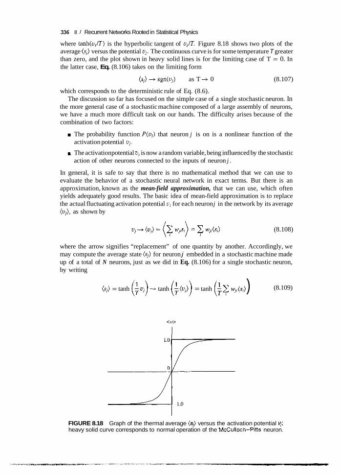
336 8 / Recurrent Networks Rooted in Statistical Physics
where tanh(u,/T) is the hyperbolic tangent of u,/T. Figure 8.18 shows two plots of the average (s,) versus the potential u,. The continuous curve is for some temperature T greater than zero, and the plot shown in heavy solid lines is for the limiting case of T = 0. In the latter case, Eq. (8.106) takes on the limiting form
(s,) + sgn(u,) as T + 0 (8.107)
which corresponds to the deterministic rule of Eq. (8.6). The discussion so far has focused on the simple case of a single stochastic neuron. In
the more general case of a stochastic machine composed of a large assembly of neurons, we have a much more difficult task on our hands. The difficulty arises because of the combination of two factors:
The probability function P(u,) that neuron j is on is a nonlinear function of the
rn The activation potential u, is now a random variable, being influenced by the stochastic
In general, it is safe to say that there is no mathematical method that we can use to evaluate the behavior of a stochastic neural network in exact terms. But there is an approximation, known as the mean-field approximation, that we can use, which often yields adequately good results. The basic idea of mean-field approximation is to replace the actual fluctuating activation potential u, for each neuron j in the network by its average (u,), as shown by
activation potential u,.
action of other neurons connected to the inputs of neuron j .
(8.108)
where the arrow signifies “replacement” of one quantity by another. Accordingly, we may compute the average state (sj) for neuron j embedded in a stochastic machine made up of a total of N neurons, just as we did in Eq. (8.106) for a single stochastic neuron, by writing
(s j ) = tanh ($u j ) + tanh ($(u j ) ) = tanh ($? wji(si) ) (8.109)
<S.> I
I
FIGURE 8.18 Graph of the thermal average (si) versus the activation potential y; heavy solid curve corresponds to normal operation of the McCulloch-Pitts neuron.
8.13 / The Mean-Field-Theory Machine 337
In light of Eq. (8.109), we may formally state the mean-field approximation as follows:
The average of some function of a random variable is approximated as the function of the average of that random variable.
For j = 1, 2, . . . , N, Eq. (8.109) represents a set of nonlinear equations with N unknowns (si) that captures the notion of noise. The solution of this set of nonlinear equations is now a manageable proposition, because the unknowns are all deterministic rather than stochastic variables, which they are in the original network.
Equation (8.109) is called the mean-field-theory equation for the average state of neuron j in a stochastic machine made up of N neurons. We may also derive this equation in a more rigorous manner using the saddle-point method, as described next.
Saddle-Point Method Let s, denote the N-by-1 state vector of a stochastic machine residing in state a. The discrete probability P, that the system is in state s, at a temperature T is given by the Boltzmann distribution of F q (8.41). The probability P, acts as a statistical weight in the sense that the average of a state-dependent function g(s,) is defined by
(8.1 10)
where the summation extends over all possible states (configurations) of the system; E, is the energy of the system in state a, and Z is the partition function defined in Eq. (8.42). For convenience of presentation, the latter definition is reproduced here as
z = exp (- $) a
(8.1 11)
Basically, mean-field approximation provides an efficient method of computing the average (g(s , ) ) . Its derivation relies on a manipulation of the summations in Eqs. (8.110) and (8.11 1).
Consider first the simple case of a stochastic neuron j with state sj. We wish to replace the discrete function g(sj> summed over sj by an integral over a pair of new continuous variables U, and V). To do so, we begin by invoking the sifing property of the Dirac delta function S(Uj), written as follows:
g(sj> = g(U, ) S(sj - U,> dUj (8.112)
Next, we use the following definition of the Dirac delta function:
(8.113)
where i is the square root of -1, and the integration with respect to vj runs over the imaginary axis. Accordingly, the use of this definition in Eq. (8.112) yields
(8.114)
338 8 / Recurrent Networks Rooted in Statistical Physics
We next use this formulation to evaluate the discrete sum of the function g(sj) over the possible values of si, and thus write
where, in the last line, we have interchanged the order of summation and integrations, and also rearranged terms. We now recognize the following identity:
= 2 cosh V,
= 2 exp(ln(cosh V,)) (8.116)
where cosh V, is the hyperbolic cosine of V,, and In denotes the natural logarithm. Hence, in light of the identity in Eq. (8.116), we may rewrite Eq. (8.115) as
(8.117)
where we have added the exponents in the integrand. Equation (8.117) is the desired result for a single stochastic neuron. It reformulates a discrete sum over two possible values of neuronal state sj = 2 1 as a double integral over two continuous variables uj and 6.
Equation (8.117) applies to a single neuron. It is a straightforward matter to extend it to a stochastic machine made up of N neurons. For this evaluation, we use the definition of the partition function Z to write
z = exp (- $) a
(8.118)
where c is a normalization constant, and E,,(U, V, T ) is the efSectiue energy, defined by
(8.119)
where U and V are both N-by-1 vectors with elements Uj and q, respectively, and the state energy E, corresponds to E(U). The elements U, and y are called the mean-fzeld variables, for reasons that will become apparent momentarily.
The effective energy E,,(U, V, T) in the exponent of the integrand in Eq. (8.118) can be large for machines with a large number of neurons. Consequently, we may solve the integral using the saddle-point method, which is a well-known technique in theoretical physics. According to this method, we recognize two things: (1) The double integral of
N
E&, V, T) = E(U) + T [U,V, - ln(cosh Y)] j = 1

8.13 / The Mean-Field-Theory Machine 339
Eq. (8.118) is dominated by saddle points in the integration intervals specified here, and (2) the saddle points of the partition function 2 will be found among the roots of the equations (Courant and Hilbert, 1970):
a - Eefi(U, V, T ) = 0 a Uj
and
a - Eefi(U, V, T ) = 0 a5
(8.120)
(8.121)
In other words, the saddle points of the partition function 2 are determined by the simultaneous stationarity of the effective energy Eeff(U, V, T ) in both of the mean field variables U, and 5. Using the definition of Eq. (8.119) in (8.120) and (8.121) yields, respectively,
1 aE(U) v. = -- I T a q
and
Uj = tanh V,
(8.122)
(8.123)
where tanh V, is the hyperbolic tangent that results from the differentiation of ln(cosh V,) with respect to V,. In general, the solutions of Eqs. (8.122) and (8.123) are real, because the effective energy E,,(U, V, T ) is real for real Uj and V,.
For a Boltzmann machine whose energy function is defined by Eq. (8.48), application of (8.122) and (8.123) yields the mean-Jeld-theory equations:
u,= tanh - c w j i u i , ( k i ) j = 1 , 2 , . . . , N (8.124)
where the state variables sj of individual neurons have been replaced by the mean-field variables Uj through the use of Eq. (8.122); the index i is not to be confused with the square root of - 1 used in Eqs. (8.1 13) to (8.1 15). It is of interest to note that the mean- field-theory equations (8.124) are the steady-state solutions of the resistance-capacitance (RC) equations:
3 = -u, + t a d , j = 1,2,. . . , N dt
(8.125)
which are seen to have a mathematical form similar to Eq. (8.2). Also, comparison of Eq. (8.124) with (8.108) immediately reveals that the mean-field variable U, is identically the same as the average state (sj). As for the other mean-field variable V,, it is identically the same as the average value of the activation potential uj . We may thus formally write
U, = (S j ) (8.126)
and
v, = (u,) (8.127)
Equations (8.126) and (8.127) justify the terminology of “mean-field variables” to describe
An important property of the effective energy function Eeff(U, V, T ) is that it has a smoother landscape than the energy function E of the original Boltzmann machine due
Uj and V,.

340 8 / Recurrent Networks Rooted in Statistical Physics
to the presence of extra terms. Consequently, there is less likelihood of getting stuck in local minima.
Mean-Field-Theory Learning Rule Thus far, we have shown how to compute the mean-field variable Uj = (s]). But, the parameters that we really need for the implementation of the Boltzmann machine are the correlations (sjsl). We may, of course, determine these correlations by formal manipulations of the partition function Z along similar lines to those we used for the derivation of Eq. (8.124). Specifically, it may be shown that (Peterson and Anderson, 1987)
(sjsi)+ qi = 2 [tanh ($? wjkUk) + tanh (+? wikUk)] (8.128)
which represents a system of N-by-N nonlinear equations for j , i = 1,2, . . . , N. For large N, we therefore have a large system of equations with deterministic variables. Experience with the computation of large systems shows that such systems, in general, tend to converge rather slowly. It is therefore tempting to go one step further in the approximation and factorize the correlation U,, as the product of two mean-field variables U, and U, as follows (Peterson and Anderson, 1987):
(8.129) (s,st) -+ UJ,+ U,U,, j , i = 1, 2, . . . , N
where U, is itself defined by Eq. (8.124). The deterministic form of Boltzmann learning in which the computation of the correla-
tions is approximate in accordance with Eqs. (8.129) and (8.124) is called mean-field- theory learning. Specifically, we may reformulate Eq. (8.75) to define the mean-jield- theory (MFT) learning rule as follows:
Aw,~ = 7(UTU: - UyU,) (8.130)
where U: and U; are the average outputs of visible neuronj (on a single pattern) in the clamped and fiee-running conditions, respectively, and 7 is the learning-rate parameter. The MFT learning algorithm is summarized in Table 8.4.
Mean-field-theory learning, as described here, is expected to improve in accuracy with increasing N, the number of neurons in the network. What is amazing, however, is that it appears to work well even for relatively small networks on the order of N = 10 neurons (Peterson and Anderson, 1987). At first glance, this observation may seem to contradict what is known about the dynamics of spin-glass models-namely, that the mean-field approximation yields relatively inaccurate results for small systems (MCzard et al., 1987). The reason why mean-field-theory learning appears to work well for small neural networks
Mean-field-theory learning is a deterministic form of Boltzmann learning, from which it is derived through the use of mean-field approximation. It therefore provides a substantial speedup over the Boltzmann machine learning procedure (Peterson and Anderson, 1987) The Boltzmann machine learning procedure performs steepest descent in the relative entropy ( H ) space if the learning-rate parameter 7 is sufficiently small, as shown in Section 8.1 1. By making 7 sufficiently small, the mean-field-theory learning proce- dure may also be made to approximate steepest descent in the H space arbitrarily closely, except at rare discontinuities (Hinton, 1989).

8.14 / Computer Experiments II 341
TABLE 8.4 Summary of the Mean-Field-Theory Learning Algorithm
1. Initialization. Initialize the network by setting the synaptic weights wji to uniformly distrib-
2. Clamping Phase. For a sequence of decreasing temperatures To, T, , . . . , T,,, solve Eq. uted random values in the range (-u, u), where a is typically 0.5 or 1.
(8.124) iteratively for the mean-field variable U, = (si ) of each free-running neuron j in the network. For this solution, use the recursion
For a clamped neuron j , simply set U, = 21 depending on whether neuron j is on or off. Hence, at the final temperature Tfind compute the clamped correlations,
where N is the total number of neurons in the network, and UT is the average output of visi- ble neuron j in the clamped phase of operation.
3. Free-Running Phase. Similarly, in the free-running phase, compute the correlations
where U,: is the average output of visible neuron j in the free-running phase of operation. 4. Weight Updating. After each input pattern has passed through steps 2 and 3, update the synap-
tic weights of the network according to the Boltzmann learning rule,
where 7 is the leaming-rate parameter.
the synaptic weights reported. 5. Iteration Until Convergence. Repeat steps 2 through 4 until there are no further changes in
8.1 4 Computer Experiments 11 Here we present the results of computer experiments on the two-dimensional mirror symmetry problem to provide two performance comparisons: (1) between Boltzmann and mean-field-theory machines, and (2) between a mean-field-theory machine and a multilayer perceptron using the relative entropy criterion; the latter network was considered in Section 6.20. As depicted in Fig. 8.19, the mirror symmetry problem requires that the network detect which one of three possible axes of symmetry is present in an N-by-N binary-pixel input pattern (Sejnowski et al., 1986).
Input patterns made up of N-by-N arrays of binary pixels are generated with one of three possible axes of symmetry: vertical, horizontal, or one of the diagonals. Only input patterns with exactly one axis of symmetry are used in the experiment. For an N-by-N array of binary pixels there are 2N*D such input patterns. The task is to train a neural network so as to classify these input patterns correctly according to their axes of symmetry. The potential difficulty in this pattern-classification problem lies in the fact that single pixels by themselves carry no information about the solution to the problem, but pairs of pixels related by a mirror symmetry can be used to extract the information needed for classification. In other words, the mirror symmetry problem is a second-order problem in the sense of Minsky and Papert (1969).

342 8 / Recurrent Networks Rooted in Statistical Physics
FIGURE 8.19 The two-dimensional mirror symmetry problem. The figure (from left to right) displays symmetry with respect to the following axes: vertical, horizontal, and a diagonal.
The results of computer experiments described here follow Peterson (1991b), using a network architecture of N-by-N input nodes, a single hidden layer of 12 neurons, and an output layer of 3 neurons (one for each axis of symmetry). The experiments were performed with two problem sizes:
4-by-4, with about 1.5 X lo3 patterns
10-by-10, with about 3.7 X 10l6 patterns
In this comparative study involving the mean-field-theory machine and multilayer perceptron, there are two subtle but important issues that need to be considered:
1. The [-I, +1] Versus [0,1] Representation. For the training of the Boltzmann and mean-field-theory machines described in this chapter, we used the [ - 1, + 11 representation for the output of a neuron. In this form of representation, both “on-on” and “off-off’’ correlations are counted as positive correlations in the learning rule of Eq. (8.75). This makes the learning faster than would be the case if we were to use the [0,1] representation, for which only the “on-on” correlations are counted. For the multilayer perceptron we also expect the [- 1, + 11 representation to allow faster learning. However, with respect to generalization, the use of [0,1] may be preferred over [- 1, + 11 in cases where two neurons are undecided-that is, their outputs have values near 0.5 and 0.0, respectively. In such a situation, the uncertainty is emphasized in the [0,1] case, whereas no learning takes place in [ - 1, + I] case. For these reasons, the [- 1, + 11 representation was chosen for both the Boltzmann and mean-field theory learning machines and the [0,1] representa- tion for the multilayer perceptron in the computer experiments reported in Peterson (199 1 b).
2. Endpoint Versus Midpoint Success Criterion. By an “endpoint” criterion we mean a success criterion in the learning process in which we require that the network provide an output Y k for the kth class whose value is fairly close to the desired (target) response. For example, in the [ - 1, + 11 representation, we may require lykl > 0.8 for the endpoint criterion. On the other hand, in the “midpoint” criterion, we simply require that the output yk be on the correct side of zero in the [- 1, + 11 representation. It turns out that the performance of the mean-field-theory machine is insensitive to such a choice because its units tend to settle to extreme states, whereas the multilayer perceptron is sensitive to it. Accordingly, in the experiments performed by Peterson (1991b), the midpoint criterion was used for the comparison of the mean-field-theory machine and multilayer perceptron.
Figures 8.20a and 8.20b compare the learning curves of the Boltzmann and mean- field-theory machines using the [ - 1, + 11 representation and the endpoint criterion for
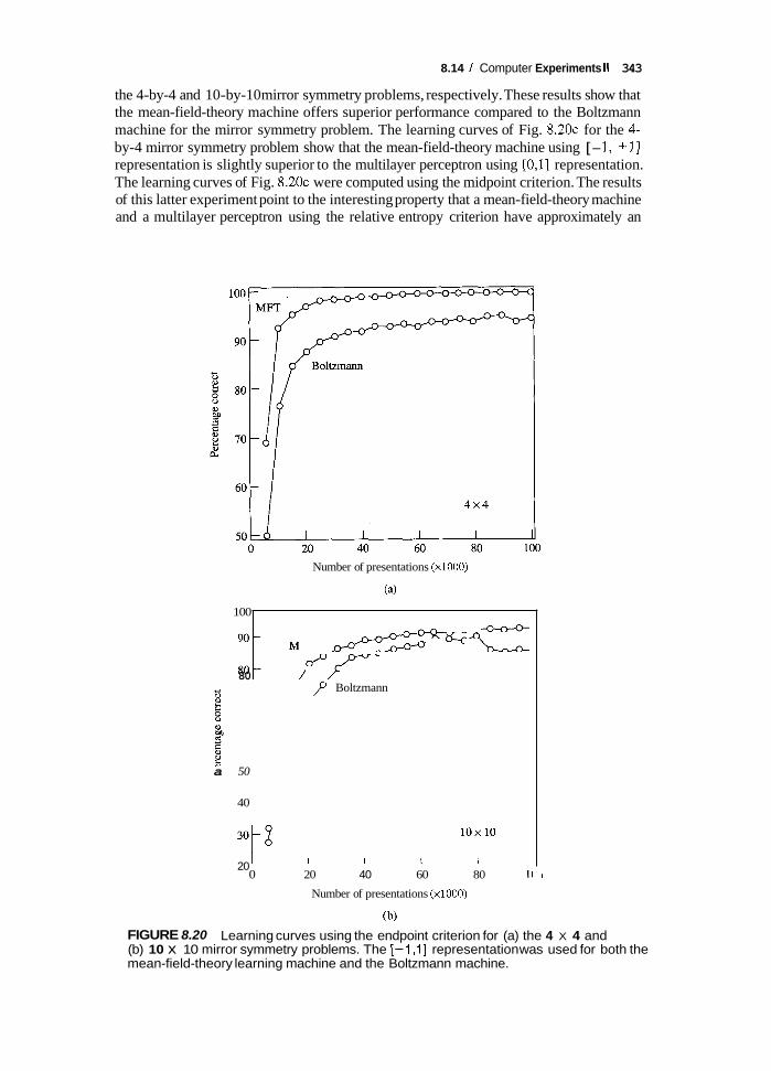
8.14 I Computer Experiments II 343
the 4-by-4 and 10-by-10 mirror symmetry problems, respectively. These results show that the mean-field-theory machine offers superior performance compared to the Boltzmann machine for the mirror symmetry problem. The learning curves of Fig. 8 . 2 0 ~ for the 4- by-4 mirror symmetry problem show that the mean-field-theory machine using [ - 1, + 11 representation is slightly superior to the multilayer perceptron using [0,1] representation. The learning curves of Fig. 8 .20~ were computed using the midpoint criterion. The results of this latter experiment point to the interesting property that a mean-field-theory machine and a multilayer perceptron using the relative entropy criterion have approximately an
Number of presentations (~1000)
(a)
100 I
901 80 c
a 50
40
/” Boltzmann
20 0 20 40 60 80 1(
Number of presentations (~1000)
(b)
I
FIGURE 8.20 Learning curves using the endpoint criterion for (a) the 4 X 4 and (b) 10 x 10 mirror symmetry problems. The [-1,1] representation was used for both the mean-field-theory learning machine and the Boltzmann machine.

344 8 I Recurrent Networks Rooted in Statistical Physics
40 0 20 40 60 80 100
Number of presentations (~1000)
(C)
FIGURE 8.20 (continued) (c) Learning curves for the midpoint criterion for the 4 X 4 mirror symmetry problem. For mean-field-theory learning the [- 1,1] representation was used and for the back-propagation learning the [0,1] representation was used. (From C. Peterson, 1991 b, with permission of Connection Science.)
equal performance if they both have a single hidden layer and the size of the input layer is much larger than that of the output layer (Peterson, 1991b). The reader is referred to Problem 8.15 for a derivation of this property.
8.1 5 Discussion In this chapter we studied a special class of recurrent networks with symmetric coupling, and whose theory is rooted in statistical physics. We first considered the Hopfield network, which employs the outer product rule (a generalization of Hebb’s postulate of learning) for setting the synaptic weights of the network. As a content-addressable memory, the Hopfield network is capable of storing no more than 0.138N random patterns, where N is the total number of neurons in the network. Various methods have been devised for increasing the storage capacity of the Hopfield network. The fact of the matter, however, is that regardless of how the synaptic weights are determined, a theoretical storage limit of 2N random patterns has been established for the class of attractor neural networks, to which the Hopfield network belongs (Gardner, 1987; Venkatesh, 1986; Cover, 1965). Cover’s separating capacity of decision surfaces, which is the basis for the theoretical storage limit of 2N patterns, was discussed in Section 7.2.
The main limitation of Hopfield networks is the lack of hidden neurons. Hidden neurons are known to learn internal representations of training patterns, thereby enhancing the performance of the neural network. The Boltzmann machine uses hidden and visible neurons that are in the form of stochastic, binary-state units. It cleverly links the simulated annealing algorithm with a neural network, and thereby exploits the beautiful properties of the Boltzmann distribution. The Boltzmann machine has some appealing features:

8.15 I Discussion 345
rn Through training, the probability distribution of the network is matched to that of the environment. This is achieved by using the relative entropy, rooted in information theory, as the measure of performance.
The network offers a generalized approach that is applicable to the basic issues of search, representation, and learning (Hinton, 1987).
The network is guaranteed to find the global minimum of the energy function, provided that the annealing schedule in the learning process is performed slowly enough (Geman and Geman, 1984).
The annealing schedule referred to here is described in Eq. (8.45). Unfortunately, this schedule is much too slow to be of practical value. In practice, a faster annealing schedule is used so as to produce reasonably good solutions, though not necessarily optimal.
The mean-field-theory machine is derived from the Boltzmann machine by analogy. Specifically, the stochastic binary-state neurons of the Boltzmann machine are replaced by deterministic analog ones. The end result is a new neural network that offers the following practical advantages (Hartman, 1991 ; Peterson and Anderson, 1987):
Being deterministic, the mean-field-theory machine is one to two orders of magnitude faster than the corresponding Boltzmann machine.
The mean-field-theory equations (8.124) are isomorphic to the steady-state solutions of the RC circuit described by Eqs. (8.125). This property, coupled with the local nature of the Boltzmann learning algorithm, makes the mean-field-theory machine a strong candidate for implementation in analog VLSI form. Indeed, Alspector et al. (1991a, b) describe a general-purpose neural network chip that can be used for implementing the mean-field-theory (and the Boltzmann) machine, on which we have more to say in Chapter 15.
w Mean-field-theory machines can be used for content-addressable memory (Alspector et al., 1992b; Hartman, 1991), pattern recognition, and combinatorial optimization problems (Peterson and Soderberg, 1989; Peterson and Anderson, 1987).
In a content-addressable memory, which we wish to discuss here, the aim is to correct errors in the state of visible neurons. Each visible neuron functions both as an input unit and an output unit of the network. The initial state of the visible neurons is determined by the input to the network, and their final state supplies the output of the network. In a Hopfield network which has no hidden neurons, retrieval proceeds simply by initializing the network and then allowing the network to evolve under its own dynamics. In the case of a mean-field-theory machine, we require a more elaborate retrieval procedure on account of the hidden neurons. Specifically, we would like to exploit the internal representation of the stored pattern learned by the hidden neurons, as an adjunct in the correction of errors in the state of visible neurons. The learning process itself needs consideration because, unlike a Boltzmann machine, a mean-field-theory machine is deterministic. In particular, a completely free-running phase is ruled out, because it is identical for all training patterns in the sense that the annealing process ends in the same single, final state. To resolve these peculiarities of learning and redeval, we may follow a robust procedure that was originally described by Hartman (1991) and applied to a general- purpose neural network chip by Alspector et al. (1992b):
rn Learning (storage). In the clamping phase, the visible neurons are all clamped to a training pattern, and the hidden neurons are updated at low temperature. In the free- running phase, half the visible neurons (picked at random) are clamped to the training pattern, and the remaining half are free.

346 8 / Recurrent Networks Rooted in Statistical Physics
Retrieval (recall). The visible neurons are clamped to a new pattern (which may include errors), thereby initializing the hidden neurons in accordance with the clamped state of the visible neurons. Then the whole network is annealed to an intermediate temperature, at which point the state of the hidden neurons approximates the learned internal representation of the stored pattern, and the visible neurons are released. Finally, the annealing process is finished, and the whole network is allowed to settle. The visible neurons are thus able to correct errors by virtue of the evoked internal representation of stored pattern learned by the hidden neurons.
It has been demonstrated by Hartman (1991) using a detailed computer simulation study and verified by Alspector et al. (1992b) using a general-purpose neural network chip that the mean-field-theory machine has a larger capacity for storage and error- correcting retrieval of random patterns than any other network. The key to this significant increase in storage capacity lies in the use of hidden neurons that assist in the storage and error-correction process. The storage capacity has also been found empirically to improve considerably with the use of more hidden neurons.
We conclude this discussion of mean-field-theory learning by summarizing its funda- mental limitations in light of a study by Gallard (1993):
1. When a supervised Boltzmann machine (i.e., one with input and output neurons) reaches thermal equilibrium, we have a probability of an output vector, given a clamped input vector that is defined previously in terms of the Boltzmann distribution. However, the analogous definition for this conditional probability in mean-field-theory learning is not similarly valid. The problem arises due to the fact that in the latter case the unclamped, interconnected hidden and output neurons of the machine in its free-running condition (i.e., negative phase) are no longer independent, and the true stochastic system is not well represented. That is, the probability of an output vector, given a clamped input vector, has different values for these two machines. The situation is made worse by adding more hidden layers or more intra-hidden-layer connections to a single-hidden-layer network. Although superficially it would seem that these additions increase the complexity potential of the functions that may be learned by a mean-field-theory machine, in reality all that the new neural connections accomplish is to erode the representational fidelity of the mean-field-theory machine. This is indeed borne out by computer simulation results.
2. Learning in a mean-field-theory machine is restricted to the simple gradient search; advanced optimization techniques such as the conjugate gradient method (discussed in Chapter 6) are of no value.
It thus appears that the use of mean-field-theory learning is restricted to neural networks with a single hidden layer, which limits the scope of their applications.
PROBLEMS
8.1 Consider a Hopfield network made up of five neurons, which is required to store the following three fundamental memories:
5, = [fl, +1, +1, +l, +1]T
gz = [+l , -1, -1, f l , -1]T
g3 = [-1, +1, -1, +1, +1]T
(a) Evaluate the 5-by-5 synaptic weight matrix of the network. (b) Demonstrate that all three fundamental memories, El , &, and &, satisfy the
alignment condition, using asynchronous updating.

Problems 347
(c) Investigate the retrieval performance of the network when it is presented with a noisy version of El in which the second element is reversed in polarity.
8.2 Investigate the use of synchronous updating for the retrieval performance of the
8.3 (a) Show that
Hopfield network described in Problem 8.1.
= [-I, -1, -1, -1, -1y
= [-1, +1, +I , -1, + 1 ] T
6 3 = [+I, -1, +1, - 1, -1]T
are also fundamental memories of the Hopfield network described in Problem 8.1. How are these fundamental memories related to those of Problem 8.1?
(b) Suppose that the first element of the fundamental memory t3 in Problem 1 is masked (Le., reduced to zero). Determine the resulting pattern produced by the Hopfield network. Compare this result with the original form of t3.
8.4 Equation (8.30) defines the synaptic weight wji produced by a modification of the outer product rule of storage. Demonstrate that a network based on this formula satisfies the alignment condition described in Eq. (8.1 1).
8.5 Consider a simple Hopfield network made up of two neurons. The synaptic weight matrix of the network is
0 -1 w=[-1 01
The threshold applied to each neuron is zero. The four possible states of the network are
s1 = [+I , +1]T
s2 = [-I, + l ] T
s3 = [-1, -1]T
sq = [+1, -1y
(a) Demonstrate that states s2 and s4 are stable, whereas states s1 and s3 exhibit a limit cycle. Do this demonstration using the following tools: 1. The alignment (stability) condition 2. The energy function
(b) What is the length of the limit cycle characterizing states s1 and s3?
8.6 Derive Eq. (8.29) defining the maximum number of fundamental memories that are all retrieved correctly by a Hopfield network with a probability of 99 percent.
8.7 Show that the energy function of a Hopfield network may be expressed as
where m, are the overlaps, defined by
where sj is the jth element of the state vector s and fundamental memory g,,.
is the jth element of the

348 8 / Recurrent Networks Rooted in Statistical Physics
8.8 In this problem we continue with the computer experiment described in Section 8.4, pertaining to the use of the Hopfield network as a content-addressable memory. The network is trained to retrieve the eight digitlike black-and-white patterns shown in Fig. 8.7, with each pattern containing 120 pixels. Continue with this computer
Initial corrupted 0 Initial corrupted 1
Initial corrupted 2 Initial corrupted 3
Initial corrupted 4 Initial corrupted 9 (a)
FIGURE P8.8 Different shades are used for the states + I and -1, compared to those in Fig. 8.7.

Problems 349
Initial compted I (b)
Initial corrupted 2
(C)
Initial corrupted 2 Initial corrupted I (d)
FIGURE P8.8 (continued)
experiment for the following situations: (a) The network is presented with initial corrupted versions of 0, 1, 2, 3, 4, 9 that
(b) The network is presented with the initial corrupted version of I shown in Fig.
(c) The network is presented with the initial corrupted version of 2 shown in Fig.
(d) The network is presented with the initial corrupted versions of I and 2 shown
8.9 (a) Derive Eq. (8.79) defining the relative entropy of a Boltzmann machine that includes input, hidden, and output neurons.
(b) Show that the Boltzmann learning rule for adjusting the synaptic weight wji in this network configuration may still be expressed in the same form as that described in Q. (8.75), with new interpretations for the correlations fi; and P,: .
are shown in Fig. P8.8a.
P8.8b.
P8.8~.
in Fig. P8.8d.

350 8 / Recurrent Networks Rooted in Statistical Physics
8.10 In light of the Markov model description of a Boltzmann machine presented in Section 8.12, investigate the unequal update rates for such a machine.
8.11 In this problem we revisit the XOR (Exclusive-OR) problem, which involves comput- ing the parity of two binary digits. The patterns of the input-output mapping are thus as follows:
Input output 00 0 01 1 10 1 11 0
From Chapter 6 on back-propagation learning and Chapter 7 on RBF networks we know that the solution to this problem requires the use of hidden neurons. So it is with the Boltzmann machine used to solve the problem. Investigate the solution of the XOR problem using the Boltzmann machine.
8.12 In this problem we use computer simulation to explore the use of the Boltzmann machine as a mechanism for solving the ‘‘424 encoder” constraint-satisfaction problem. The encoder represents the task of two processes communicating informa- tion through a link of restricted bandwidth. Figure P8.12 depicts the topology of the 424 encoder network. The problem specifies four visible input-output neurons (Vl) representing process 1, a second set of four visible input-output neurons (V2) representing process 2, and two hidden neurons ( H ) representing a parallel communication link of limited bandwidth. The problem further specifies that each of the processes must be capable of transmittingheceiving four unique patterns {(lOOO), (OlOO), (OOlO), (0001)). Since the two processes are not directly connected, which is a limitation of the problem, the minimum number of hidden neurons required for perfect communication is log, u, where u is the number of unique patterns.
0
0
0
0
0
0
0
0
0
0 Input Hidden output layer layer layer
FIGURE P8.12
Problems 351
The purpose of the experiment is to reproduce the results for the 424 encoder problem presented by Ackley et al. (1985) under the following specifications: (a) Twenty random binary input vectors from the set {(lOOO), (OlOO), (OOlO),
(0001)); noise is added to the vectors with a probability of 0.15 that “on” bits are turned “off,” and a probability of 0.05 that “off” bits are turned “on.” The addition of noise is intended to prevent the synaptic weights from growing too large.
(b) Number of updates = 10, such that, on the average, all neurons are updated on each annealing cycle.
(c) Annealing schedule:
(2 @ 20, 2 @ 15, 2 @ 12,4 @ 10, 2 @ 20, 2 @ 15, 2 @ 12, 4 @ lo}
8.13 Using the saddle-point method, derive the formula for the correlation (sJ~) given in Eq. (8.128) for mean-field-theory learning.
8.14 The Boltzmann machine performs gradient descent (in weight space) on the relative entropy between the underlying probability distribution of the environment and the probability distribution learned by the network. On what function does the mean- field-theory machine perform its gradient descent? You may refer to Hinton (1989) for a discussion of this issue.
8.15 Consider a network architecture consisting of an input layer, a single hidden layer, and an output layer. The size of the input layer is much larger than that of the output layer. Consequently, in the case of a mean-field-theory machine we may say that insofar as a hidden neuron is concerned, the feedback signal from an output neuron has a minor influence compared to the feedforward signal from an input neuron. For such a network architecture, show that the mean-field-theory machine has a behavior approximately the same as that of a multilayer perceptron using the relative entropy criterion; the latter network was considered in Section 6.20. In particular, show that for these two different neural networks: (a) The update formulas for the synaptic weights of an output neuron have the same
(b) Likewise, the update formulas for the synaptic weights of a hidden neuron have
8.16 Consider a recurrent network that is asymmetric in that w, # wJz. Show that the mean-field-theory learning algorithm will automatically symmetrize the network provided that, after each weight update, each weight is decayed toward zero by a small amount proportional to its magnitude (Hinton, 1989).
approximate form.
the same approximate form.