Embed Size (px)
Citation preview
Recursion aware modeling and discovery for hierarchicalsoftware event log analysis (extended)Citation for published version (APA):Leemans, M., van der Aalst, W. M. P., & van den Brand, M. G. J. (2017). Recursion aware modeling anddiscovery for hierarchical software event log analysis (extended). arXiv, 1-14. [1710.09323v1].https://arxiv.org/abs/1710.09323
Document status and date:Published: 17/10/2017
Document Version:Publisher’s PDF, also known as Version of Record (includes final page, issue and volume numbers)
Please check the document version of this publication:
• A submitted manuscript is the version of the article upon submission and before peer-review. There can beimportant differences between the submitted version and the official published version of record. Peopleinterested in the research are advised to contact the author for the final version of the publication, or visit theDOI to the publisher's website.• The final author version and the galley proof are versions of the publication after peer review.• The final published version features the final layout of the paper including the volume, issue and pagenumbers.Link to publication
General rightsCopyright and moral rights for the publications made accessible in the public portal are retained by the authors and/or other copyright ownersand it is a condition of accessing publications that users recognise and abide by the legal requirements associated with these rights.
• Users may download and print one copy of any publication from the public portal for the purpose of private study or research. • You may not further distribute the material or use it for any profit-making activity or commercial gain • You may freely distribute the URL identifying the publication in the public portal.
If the publication is distributed under the terms of Article 25fa of the Dutch Copyright Act, indicated by the “Taverne” license above, pleasefollow below link for the End User Agreement:www.tue.nl/taverne
Take down policyIf you believe that this document breaches copyright please contact us at:[email protected] details and we will investigate your claim.
Download date: 31. Mar. 2022
Recursion Aware Modeling and DiscoveryFor Hierarchical Software Event Log Analysis (Ext.)
Technical Report version with guarantee proofs for the discovery algorithms
Maikel LeemansEindhoven University of Technology
Eindhoven, The NetherlandsEmail: [email protected]
Wil M. P. van der AalstEindhoven University of Technology
Eindhoven, The NetherlandsEmail: [email protected]
Mark G. J. van den BrandEindhoven University of Technology
Eindhoven, The NetherlandsEmail: [email protected]
Abstract—This extended paper presents 1) a novel hierarchyand recursion extension to the process tree model; and 2)the first, recursion aware process model discovery techniquethat leverages hierarchical information in event logs, typicallyavailable for software systems. This technique allows us toanalyze the operational processes of software systems under real-life conditions at multiple levels of granularity. The work can bepositioned in-between reverse engineering and process mining.An implementation of the proposed approach is available as aProM plugin. Experimental results based on real-life (software)event logs demonstrate the feasibility and usefulness of theapproach and show the huge potential to speed up discoveryby exploiting the available hierarchy.
Keywords-Reverse Engineering; Process Mining; RecursionAware Discovery; Event Log; Hierarchical Event Log; ProcessDiscovery; Hierarchical Discovery; Hierarchical Modeling
I. INTRODUCTION
System comprehension, analysis, maintenance, and evo-lution are largely dependent on information regarding thestructure, behavior, operation, and usage of software systems.To understand the operation and usage of a system, one hasto observe and study the system “on the run”, in its natural,real-life production environment. To understand and maintainthe (legacy) behavior when design and documentation aremissing or outdated, one can observe and study the system in acontrolled environment using, for example, testing techniques.In both cases, advanced algorithms and tools are needed tosupport a model driven reverse engineering and analysis ofthe behavior, operation, and usage. Such tools should be ableto support the analysis of performance (timing), frequency(usage), conformance and reliability in the context of a behav-ioral backbone model that is expressive, precise and fits theactual system. This way, one obtains a reliable and accurateunderstanding of the behavior, operation, and usage of thesystem, both at a high-level and a fine-grained level.
The above design criteria make process mining a goodcandidate for the analysis of the actual software behavior.Process mining techniques provide a powerful and mature wayto discover formal process models and analyze and improvethese processes based on event log data from the system [46].Event logs show the actual behavior of the system, and couldbe obtained in various ways, like, for example, instrumentationtechniques. Numerous state of the art process mining tech-niques are readily available and can be used and combined
through the Process Mining Toolkit ProM [53]. In addition,event logs are backed by the IEEE XES standard [22], [53].
Typically, the run-time behavior of a system is large andcomplex. Current techniques usually produce flat models thatare not expressive enough to master this complexity and areoften difficult to understand. Especially in the case of softwaresystems, there is often a hierarchical, possibly recursive,structure implicitly reflected by the behavior and event logs.This hierarchical structure can be made explicit and should beused to aid model discovery and further analysis.
In this paper, we 1) propose a novel hierarchy and recursionextension to the process tree model; and 2) define the first,recursion aware process model discovery technique that lever-ages hierarchical information in event logs, typically availablefor software systems. This technique allows us to analyzethe operational processes of software systems under real-lifeconditions at multiple levels of granularity. In addition, theproposed technique has a huge potential to speed up discoveryby exploiting the available hierarchy. An implementation ofthe proposed algorithms is made available via the Statechartplugin for ProM [30]. The Statechart workbench provides anintuitive way to discover, explore and analyze hierarchicalbehavior, integrates with existing ProM plugins and links backto the source code in Eclipse.
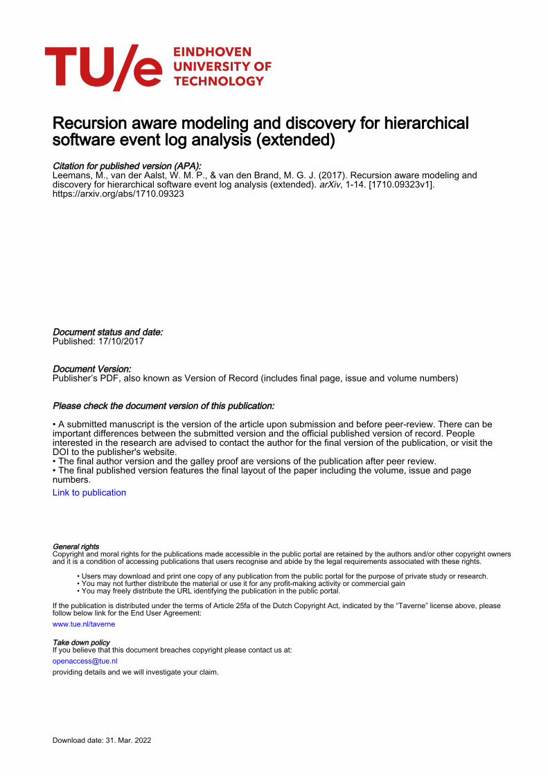
This paper is organized as follows (see Figure 1). Section IIpositions the work in existing literature. Section III presentsformal definitions of the input (event logs) and the proposednovel hierarchical process trees. In Section IV, we discusshow to obtain an explicit hierarchical structure. Two proposednovel, hierarchical process model discovery techniques areexplained in Section V. In Section VI, we show how to filter,annotate, and visualize our hierarchical process trees. Theapproach is evaluated in Section VII using experiments anda small demo. Section VIII concludes the paper.
Fig. 1. Outline of the paper and our discovery approach.
arX
iv:1
710.
0932
3v1
[cs
.SE
] 1
7 O
ct 2
017
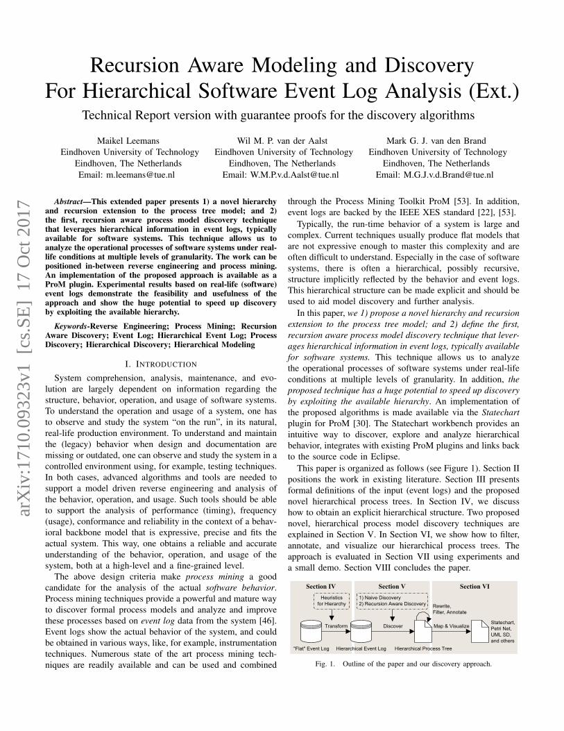
TABLE ICOMPARISON OF RELATED TECHNIQUES AND THE EXPRESSIVENESS OF THE RESULTING MODELS, DIVIDED INTO THE GROUPS FROM SECTION II.
Author Technique / Toolkit Input Formalism
Execution Semantics
Model Quality
Aggregate Runs
Frequency Info
Performance InfoChoice
Loop
Concurrency
Hierarchy
Named Submodels
Recursion
Stat
icA
naly
sis [45] Tonella Object flow analysis C++ source code UML Interact. - n/a n/a - - - - - - - -
[27] Kollmann Java code structures Java source code UML Collab. - n/a n/a - - - - - - - -[28] Korshunova CPP2XMI, SQuADT C++ source code UML SD, AD - n/a n/a - - X X - - - -[40] Rountev Dataflow analysis Java source code UML SD ±1 n/a n/a - - X X - - - -[4] Amighi Sawja framework Java byte code CFG - n/a n/a - - X X - - - -
Dyn
amic
Ana
lysi
s
[3] Alalfi PHP2XMI Instrumentation UML SD ±1 - - - - - - - - - -[39] Oechsle JAVAVIS Java debug interface UML SD ±1 - - - - - - X - - -[11] Briand Meta models / OCL Instrumentation UML SD ±1 - - - - X X - - - -[10] Briand Meta models / OCL Instrumentation UML SD ±1 - - - - X X X - - -[29] Labiche Meta models / OCL Instrumentation + source UML SD ±1 - - - - X X - - - -[44] Systa Shimba Customized debugger SD variant ±1 - - - - X X - - - -[55] Walkinshaw MINT Log with traces EFSM X X X - - X X - - - -[8] Beschastnikh CSight Given log, instrument CFSM X X X - - X X X - - -[1] Ackermann Behavior extraction Monitor network packets UML SD ±1 - X - X X X - - - -[20] Graham gprof profiler Instrumentation Call graphs - - - - X - - - X X ±8
[17] De Pauw Execution patterns Program Trace Exec. Pattern - - - X - - X - X X X[7] Beschastnikh Synoptic Log with traces FSM X X X X - X X - - - -[23] Heule DFAsat Log with traces DFA X X X - - X X - - - -
Gra
mm
ar [38] Nevill-Manning Sequitur Symbol sequence Grammar X - - - - - - - X - -[41] Siyari Lexis Symbol sequence Lexis-DAG X - X - - - - - X - -[26] Jonyer SubdueGL Symbol Graph Graph Grammar X - - - - X - - X - ±9
Proc
ess
Min
ing
[49] Van der Aalst Alpha algorithm Event Log Petri net X - X X2 X2 X X X - - -[48] Van der Aalst Theory of Regions Event Log Petri net X - X X2 X2 X X X - - -[56] Weijters Flexible heuristics miner Event Log Heuristics net X - X X2 X2 X X X - - -[50] Werf, van der ILP miner Event Log Petri net X X X X2 X2 X X X - - -[52] Zelst, S. J. van ILP with filtering Event Log Petri net X X X X2 X2 X X X - - -[47] Alves de Medeiros Genetic Miner Event Log Petri net X X X X2 X2 X X X - - -[12] Buijs ETM algorithm Event Log Process tree X X X X2 X2 X X X - - -[35] Leemans S.J.J. Inductive Miner Event Log Process tree X X X X2 X2 X X X - - -[21] Gunther Fuzzy Miner Event Log Fuzzy model - - X X3 - X X4 - X - -[25] Bose Two-phase discovery Event Log Fuzzy model - - X X3 - X X5 - X - -[15] Conforti BPMN miner Event Log BPMN X X X ±2 ±2 X X6 X X - -
This paper Recursion Aware Disc. Event Log H. Process tree* X X X X2 X2 X X7 X X X X
1 Formal semantics are available for UML SD variants.2 Aligning an event log and a process model enables advanced performance,frequency, and conformance analysis, as described in [2], [35].3 Various log-based process metrics have been defined which capture differentnotions of frequency, significance, and correlation [21].4 The hierarchy is based on anonymous clusters in the resulting model [21].
5 The hierarchy is based on abstraction patterns over events [24], [25].6 The hierarchy is based on discovered relations over extra data in the event log.7 The hierarchy is based on the hierarchical information in the event log.8 Recursion is detectable as a cycle, but without performance analysis support.9 Only tail recursion is supported.* Hierarchical process tree, as introduced in Definition III.3.
II. RELATED WORK
Substantial work has been done on constructing modelsfrom software or example behavior in a variety of researchdomains. This section presents a brief comparison of variousapproaches and focuses mainly on the design criteria from theintroduction. That is, the approach and tools should providea behavioral backbone model that is expressive, precise andfits the actual system, and ideally should be able to supportat least performance (timing) and frequency (usage) analysis.Table I summarizes the comparison.
A. Groups and Criteria for Comparison
We have divided the related work into four groups. StaticAnalysis utilizes static artifacts like source code files. DynamicAnalysis utilizes runtime information through instrumentationor tracing interfaces like debuggers. Grammar Inference relieson example behavior in the form of abstract symbol sequences.
Process Mining relies on events logs and is in that sense a moreimplementation or platform agnostic approach.
For the comparison on design criteria, we define three setsof features. Firstly, a precise and fit model should: a) haveformal execution semantics, and b) the underlying discoveryalgorithm should either guarantee or allow the user to con-trol the model quality. The quality of a model is typicallymeasured in terms of metrics like fitness and precision, butother qualities (e.g., simplicity and generalization) can alsobe considered [46]. Fitness expresses the part of the log (c.q.system behavior) that is represented by the model; precisionexpresses the behavior in the model that is present in thelog (c.q. system behavior). Secondly, the model should beused as the backbone for further analysis. At the very least,frequency (usage) and performance (timing) analysis shouldbe supported. In addition, the analysis should be (statistically)significant, and hence the technique should be able to aggre-gate information over multiple execution runs. Thirdly, the
model should be expressive and be able to capture the typeof behavior encountered in software system cases. Not onlyshould branching behavior like choices (e.g., if-then-else) andloops (e.g., foreach, iterators) be supported, but also hierarchyand recursion. Furthermore, for hierarchies, meaningful namesfor the different submodels are also important.
B. Discussion of the Related Work
In general, static and symbolic analysis of software hasdifficulty capturing the actual, dynamic behavior; especially inthe case of dynamic types (e.g., inheritance, dynamic binding,exception handling) and jumps. In these cases, it is oftenfavorable to observe the actual system for the behavior. Sincestatic techniques either unfold or do not explore function calls,they lack support for recursive behavior. In addition, becausethese techniques only look at static artifacts, they lack anyform of timing or usage analysis.
In the area of dynamic analysis, the focus is on obtaininga rich but flat control flow model. A lot of effort has beenput in enriching models with more accurate choice and loopinformation, guards, and other predicates. However, notionsof recursion or preciseness of models, or application of thesemodels, like for analysis, seems to be largely ignored. Thefew approaches that do touch upon performance or frequencyanalysis ([1], [17], [20]) do so with models lacking formalsemantics or model quality guarantees.
In contrast to dynamic analysis techniques, grammar infer-ence approaches are actively looking for repeating sub patterns(i.e., sources for hierarchies). The used grammars have a strongformal basis. However, in the grammar inference domain,abstract symbols are assumed as input, and the notion ofbranching behavior (e.g., loops) or analysis is lost.
In the area of process mining, numerous techniques havebeen proposed. These techniques have strong roots in Petrinets, model conversions, and alignment-based analysis [2],[35] Process mining techniques yield formal models directlyusable for advanced performance, frequency and conformanceanalysis. There are only a few techniques in this domainthat touch upon the subject of hierarchies. In [21], [25], ahierarchy of anonymous clusters is created based on behavioralabstractions. The hierarchy of anonymous clusters in [15]is based on functional and inclusion dependency discoverytechniques over extra data in the event log. None of thesetechniques yields named submodels or supports recursion.
Process mining techniques rely on event logs for their input.These event logs can easily be obtained via the same tech-niques used by dynamic analysis for singular and distributedsystems [34]. Example techniques include, but are not limitedto, Java Agents, Javassist [13], [14], AspectJ [19], AspectC++[42], AOP++ [57] and the TXL preprocessor [16].
III. DEFINITIONS
Before we explain the proposed discovery techniques, wefirst introduce the definitions for our input and internalrepresentation. We start with some preliminaries in Subsec-tion III-A. In Subsection III-B we introduce two types of event
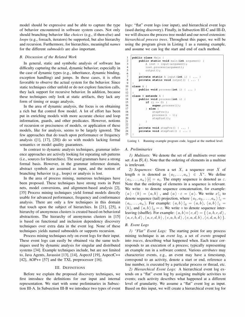
logs: “flat” event logs (our input), and hierarchical event logs(used during discovery). Finally, in Subsection III-C and III-D,we will discuss the process tree model and our novel extension:hierarchical process trees. Throughout this paper, we will beusing the program given in Listing 1 as a running example,and assume we can log the start and end of each method.
1 public class Main {2 public static void main(int argument) {3 A inst = input(argument);4 inst.process(argument);5 output();6 }7 private static A input(int i) { ... }8 private static void output() { ... }9 }
10 class A {11 public void process(int i) { ... }12 }13 class B extends A {14 public void process(int i) {15 if (i <= 0) {16 super.process(i);17 } else {18 stepPre();19 process(i - 1);20 stepPost();21 }22 }23 private void stepPre() { ... }24 private void stepPost() { ... }25 }
Listing 1. Running example program code, logged at the method level.
A. Preliminaries
1) Multisets: We denote the set of all multisets over someset A as B(A). Note that the ordering of elements in a multisetis irrelevant.
2) Sequences: Given a set X , a sequence over X oflength n is denoted as 〈 a1, . . . , an 〉 ∈ X∗. We define〈 a1, . . . , an 〉 [i] = ai. The empty sequence is denoted as ε.Note that the ordering of elements in a sequence is relevant.We write · to denote sequence concatenation, for example:〈 a 〉 · 〈 b 〉 = 〈 a, b 〉 , and 〈 a 〉 · ε = 〈 a 〉. We write x�i todenote sequence (tail) projection, where 〈 a1, a2, . . . , an 〉 �i =〈 ai, . . . , an 〉. For example: 〈 a, b 〉 �0 = 〈 a, b 〉, 〈 a, b 〉 �1 =〈 b 〉, and 〈 a, b 〉 �2 = ε. We write � to denote sequence inter-leaving (shuffle). For example: 〈 a, b 〉�〈 c, d 〉 = { 〈 a, b, c, d 〉 ,〈 a, c, b, d 〉 , 〈 a, c, d, b 〉 , 〈 c, a, b, d 〉 , 〈 c, a, d, b 〉 , 〈 c, d, a, b 〉 }.
B. Event Logs
1) “Flat” Event Logs: The starting point for any processmining technique is an event log, a set of events groupedinto traces, describing what happened when. Each trace cor-responds to an execution of a process; typically representingan example run in a software context. Various attributes maycharacterize events, e.g., an event may have a timestamp,correspond to an activity, denote a start or end, reference aline number, is executed by a particular process or thread, etc.
2) Hierarchical Event Logs: A hierarchical event log ex-tends on a “flat” event log by assigning multiple activities toevents; each activity describes what happened at a differentlevel of granularity. We assume a “flat” event log as input.Based on this input, we will create a hierarchical event log for
discovery. For the sake of clarity, we will ignore most eventattributes, and use sequences of activities directly, as definedbelow.
Definition III.1 (Hierarchical Event Log):Let A be a set of activities. Let L ∈ B((A∗)
∗) be a
hierarchical event log, a multiset of traces. A trace t ∈ L,with t ∈ (A∗)
∗, is a sequence of events. Each event x ∈ t,with x ∈ A∗, is described by a sequence of activities, statingwhich activity was executed at each level in the hierarchy. y
Consider, for example, the hierarchical event log L =[ 〈 〈 g, a 〉 , 〈 g, b 〉 , 〈 c 〉 〉 ]. This log has one trace, where thefirst event is labeled 〈 g, a 〉, the second event is labeled〈 g, b 〉, and the third event is labeled 〈 c 〉. For the sake ofreadability, we will use the following shorthand notation:L = [ 〈 g.a, g.b, c 〉 ]. In this example log, we have two levelsin our hierarchy: the longest event label has length 2, notation:‖L‖ = 2. Complex behavior, like choices, loops and parallel(interleaved) behavior, is typically represented in an event logvia multiple (sub)traces, showing the different execution paths.
We write the following to denote hierarchy concatenation:f. 〈 g.a, g.b, c 〉 = 〈 f.g.a, f.g.b, f.c 〉. We generalize concate-nation to hierarchical logs: f.L = [ f.t | t ∈ L ].
We extend sequence projection to hierarchical traces andlogs, such that a fixed length prefix is removed for all events:〈 g.a, g.b, c 〉 �∗0 = 〈 g.a, g.b, c 〉, 〈 g.a, g.b, c 〉 �∗1 = 〈 a, b 〉,〈 g.a, g.b, c 〉 �∗2 = ε. For logs: L�∗i = [ t�∗i | t ∈ L ].
In Table II, an example hierarchical trace is shown. Here,we used the class plus method name as activities. Whilegenerating logs, one could also include the full packagename (i.e., a canonical name), method parameter signature (todistinguish overloaded methods), and more.
C. Process TreesIn this subsection, we introduce process trees as a notation
to compactly represent block-structured models. An importantproperty of block-structured models is that they are sound byconstruction; they do not suffer from deadlocks, livelocks, andother anomalies. In addition, process trees are tailored towardsprocess discovery and have been used previously to discoverblock-structured workflow nets [35]. A process tree describesa language; an operator describes how the languages of itssubtrees are to be combined.
Definition III.2 (Process Tree):We formally define process trees recursively. We assume afinite alphabet A of activities and a set
⊗of operators to be
given. Symbol τ /∈ A denotes the silent activity.• a with a ∈ (A ∪ { τ }) is a process tree;• Let P1, . . . , Pn with n > 0 be process trees and let ⊗ ∈⊗
be a process tree operator, then ⊗(P1, . . . , Pn) is aprocess tree.
We consider the following operators for process trees:→ denotes the sequential execution of all subtrees× denotes the exclusive choice between one of the subtrees denotes the structured loop of loop body P1 and alterna-
tive loop back paths P2, . . . , Pn (with n ≥ 2)∧ denotes the parallel (interleaved) execution of all subtrees
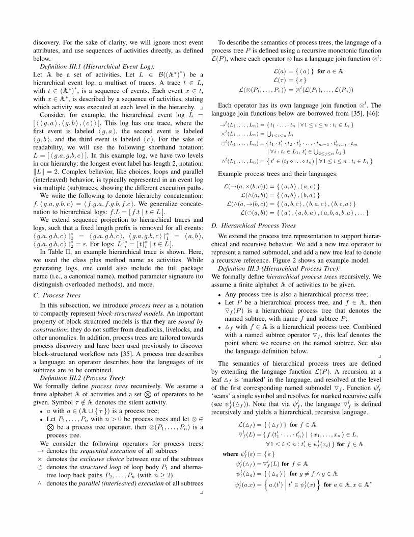
y
To describe the semantics of process trees, the language of aprocess tree P is defined using a recursive monotonic functionL(P ), where each operator ⊗ has a language join function ⊗l:
L(a) = { 〈 a 〉 } for a ∈ AL(τ) = { ε }
L(⊗(P1, . . . , Pn)) = ⊗l(L(P1), . . . ,L(Pn))
Each operator has its own language join function ⊗l. Thelanguage join functions below are borrowed from [35], [46]:
→l(L1, . . . , Ln) = { t1 · . . . · tn | ∀1 ≤ i ≤ n : ti ∈ Li }×l(L1, . . . , Ln) =
⋃1≤i≤n Li
l(L1, . . . , Ln) = { t1 · t′1 · t2 · t′2 · . . . · tm−1 · t′m−1 · tm| ∀ i : ti ∈ L1, t′i ∈
⋃2≤j≤n Lj }
∧l(L1, . . . , Ln) ={t′ ∈ (t1 � . . . � tn)
∣∣ ∀1 ≤ i ≤ n : ti ∈ Li
}Example process trees and their languages:
L(→(a,×(b, c))) = { 〈 a, b 〉 , 〈 a, c 〉 }L(∧(a, b)) = { 〈 a, b 〉 , 〈 b, a 〉 }
L(∧(a,→(b, c)) = { 〈 a, b, c 〉 , 〈 b, a, c 〉 , 〈 b, c, a 〉 }L((a, b)) = { 〈 a 〉 , 〈 a, b, a 〉 , 〈 a, b, a, b, a 〉 , . . . }
D. Hierarchical Process Trees
We extend the process tree representation to support hierar-chical and recursive behavior. We add a new tree operator torepresent a named submodel, and add a new tree leaf to denotea recursive reference. Figure 2 shows an example model.
Definition III.3 (Hierarchical Process Tree):We formally define hierarchical process trees recursively. Weassume a finite alphabet A of activities to be given.• Any process tree is also a hierarchical process tree;• Let P be a hierarchical process tree, and f ∈ A, thenOf (P ) is a hierarchical process tree that denotes thenamed subtree, with name f and subtree P ;
• Mf with f ∈ A is a hierarchical process tree. Combinedwith a named subtree operator Of , this leaf denotes thepoint where we recurse on the named subtree. See alsothe language definition below.
yThe semantics of hierarchical process trees are defined
by extending the language function L(P ). A recursion at aleaf Mf is ‘marked’ in the language, and resolved at the levelof the first corresponding named submodel Of . Function ψlf‘scans’ a single symbol and resolves for marked recursive calls(see ψl
f (Mf )). Note that via ψlf , the language Olf is definedrecursively and yields a hierarchical, recursive language.
L(Mf ) = { 〈Mf 〉 } for f ∈ AOl
f (L) = { f.(t′1 · . . . · t′n) | 〈x1, . . . , xn 〉 ∈ L,∀1 ≤ i ≤ n : t′i ∈ ψl
f (xi) } for f ∈ Awhere ψl
f (ε) = { ε }ψl
f (Mf ) =Olf (L) for f ∈ A
ψlf (Mg) = { 〈Mg 〉 } for g 6= f ∧ g ∈ A
ψlf (a.x) =
{a.(t′)
∣∣∣ t′ ∈ ψlf (x)
}for a ∈ A, x ∈ A∗
Example hierarchical process trees and their languages:
L(Of (→(a, b)) = { 〈 f.a, f.b 〉 }L(Of (→(a,Og(b))) = { 〈 f.a, f.g.b 〉 }
L(Of (×(→(a,Mf ), b)) = { 〈 f.b 〉 , 〈 f.a, f.f.b 〉 ,〈 f.a, f.f.a, f.f.f.b 〉 , . . . }
L(Of (Og(×(a,Mf ))) = { 〈 f.g.a 〉 , 〈 f.g.f.g.a 〉 ,〈 f.g.f.g.f.g.a 〉 , . . . }
L(Of (Og(×(a,Mf ,Mg))) = { 〈 f.g.a 〉 , 〈 f.g.g.a 〉 , 〈 f.g.f.g.a 〉 ,〈 f.g.f.g.g.a 〉 , 〈 f.g.g.f.g.a 〉 , . . . }
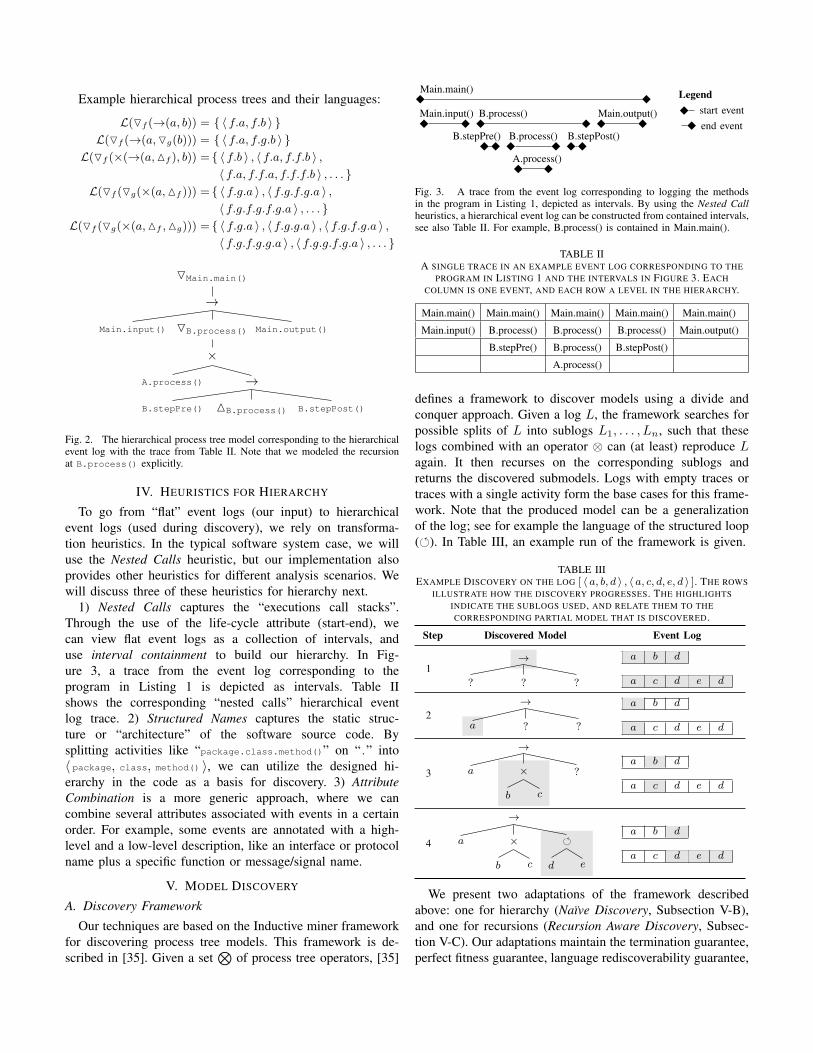
OMain.main()
→
Main.input() OB.process()
×
A.process() →
B.stepPre() MB.process() B.stepPost()
Main.output()
Fig. 2. The hierarchical process tree model corresponding to the hierarchicalevent log with the trace from Table II. Note that we modeled the recursionat B.process() explicitly.
IV. HEURISTICS FOR HIERARCHY
To go from “flat” event logs (our input) to hierarchicalevent logs (used during discovery), we rely on transforma-tion heuristics. In the typical software system case, we willuse the Nested Calls heuristic, but our implementation alsoprovides other heuristics for different analysis scenarios. Wewill discuss three of these heuristics for hierarchy next.
1) Nested Calls captures the “executions call stacks”.Through the use of the life-cycle attribute (start-end), wecan view flat event logs as a collection of intervals, anduse interval containment to build our hierarchy. In Fig-ure 3, a trace from the event log corresponding to theprogram in Listing 1 is depicted as intervals. Table IIshows the corresponding “nested calls” hierarchical eventlog trace. 2) Structured Names captures the static struc-ture or “architecture” of the software source code. Bysplitting activities like “package.class.method()” on “.” into〈 package, class, method() 〉, we can utilize the designed hi-erarchy in the code as a basis for discovery. 3) AttributeCombination is a more generic approach, where we cancombine several attributes associated with events in a certainorder. For example, some events are annotated with a high-level and a low-level description, like an interface or protocolname plus a specific function or message/signal name.
V. MODEL DISCOVERY
A. Discovery Framework
Our techniques are based on the Inductive miner frameworkfor discovering process tree models. This framework is de-scribed in [35]. Given a set
⊗of process tree operators, [35]
Legendstart eventend event
Main.main()
Main.input() B.process() Main.output()
B.stepPre() B.process() B.stepPost()
A.process()
Fig. 3. A trace from the event log corresponding to logging the methodsin the program in Listing 1, depicted as intervals. By using the Nested Callheuristics, a hierarchical event log can be constructed from contained intervals,see also Table II. For example, B.process() is contained in Main.main().
TABLE IIA SINGLE TRACE IN AN EXAMPLE EVENT LOG CORRESPONDING TO THE
PROGRAM IN LISTING 1 AND THE INTERVALS IN FIGURE 3. EACHCOLUMN IS ONE EVENT, AND EACH ROW A LEVEL IN THE HIERARCHY.
Main.main() Main.main() Main.main() Main.main() Main.main()
Main.input() B.process() B.process() B.process() Main.output()
B.stepPre() B.process() B.stepPost()
A.process()
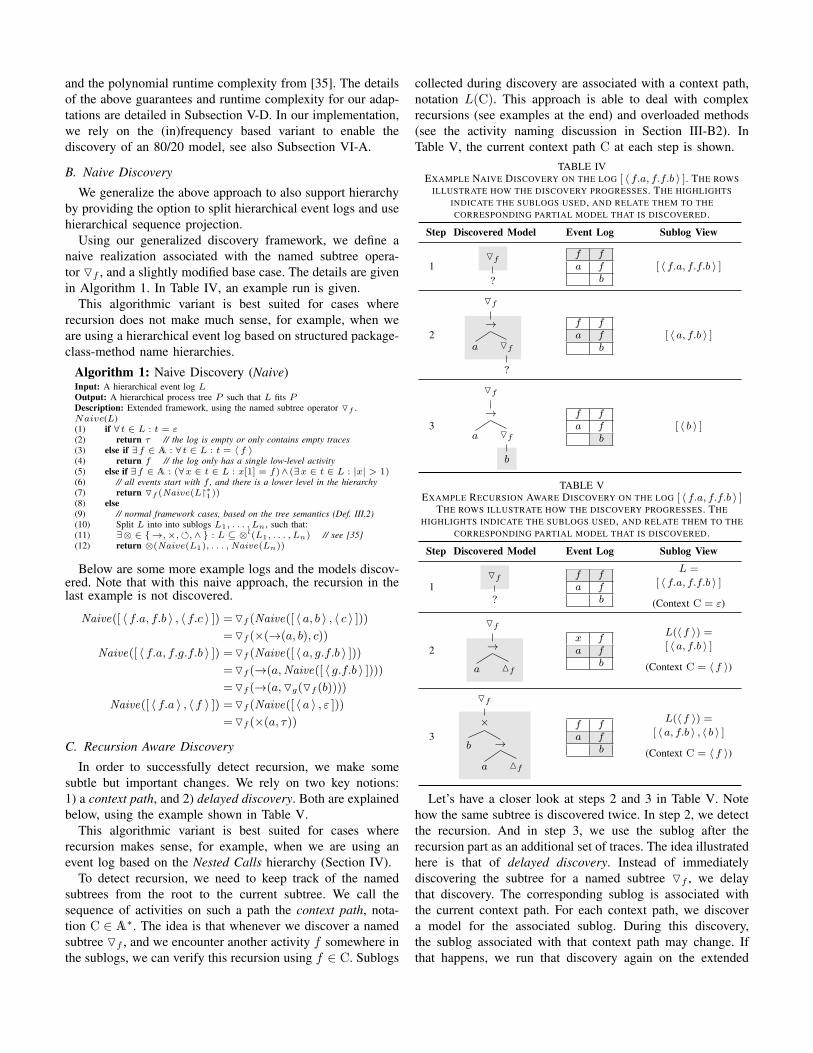
defines a framework to discover models using a divide andconquer approach. Given a log L, the framework searches forpossible splits of L into sublogs L1, . . . , Ln, such that theselogs combined with an operator ⊗ can (at least) reproduce Lagain. It then recurses on the corresponding sublogs andreturns the discovered submodels. Logs with empty traces ortraces with a single activity form the base cases for this frame-work. Note that the produced model can be a generalizationof the log; see for example the language of the structured loop(). In Table III, an example run of the framework is given.
TABLE IIIEXAMPLE DISCOVERY ON THE LOG [ 〈 a, b, d 〉 , 〈 a, c, d, e, d 〉 ]. THE ROWS
ILLUSTRATE HOW THE DISCOVERY PROGRESSES. THE HIGHLIGHTSINDICATE THE SUBLOGS USED, AND RELATE THEM TO THECORRESPONDING PARTIAL MODEL THAT IS DISCOVERED.
Step Discovered Model Event Log
1→
? ? ?
a b d
a c d e d
2→
a ? ?
a b d
a c d e d
3
→
a ×
b c
?a b d
a c d e d
4
→
a ×
b c
d e
a b d
a c d e d
We present two adaptations of the framework describedabove: one for hierarchy (Naıve Discovery, Subsection V-B),and one for recursions (Recursion Aware Discovery, Subsec-tion V-C). Our adaptations maintain the termination guarantee,perfect fitness guarantee, language rediscoverability guarantee,
and the polynomial runtime complexity from [35]. The detailsof the above guarantees and runtime complexity for our adap-tations are detailed in Subsection V-D. In our implementation,we rely on the (in)frequency based variant to enable thediscovery of an 80/20 model, see also Subsection VI-A.
B. Naive Discovery
We generalize the above approach to also support hierarchyby providing the option to split hierarchical event logs and usehierarchical sequence projection.
Using our generalized discovery framework, we define anaive realization associated with the named subtree opera-tor Of , and a slightly modified base case. The details are givenin Algorithm 1. In Table IV, an example run is given.
This algorithmic variant is best suited for cases whererecursion does not make much sense, for example, when weare using a hierarchical event log based on structured package-class-method name hierarchies.
Algorithm 1: Naive Discovery (Naive)Input: A hierarchical event log LOutput: A hierarchical process tree P such that L fits PDescription: Extended framework, using the named subtree operator Of .Naive(L)(1) if ∀ t ∈ L : t = ε(2) return τ // the log is empty or only contains empty traces(3) else if ∃f ∈ A : ∀ t ∈ L : t = 〈 f 〉(4) return f // the log only has a single low-level activity(5) else if ∃f ∈ A : (∀x ∈ t ∈ L : x[1] = f)∧(∃x ∈ t ∈ L : |x| > 1)(6) // all events start with f , and there is a lower level in the hierarchy(7) return Of (Naive(L�∗1))(8) else(9) // normal framework cases, based on the tree semantics (Def. III.2)(10) Split L into into sublogs L1, . . . , Ln, such that:(11) ∃⊗ ∈ {→,×,,∧} : L ⊆ ⊗l(L1, . . . , Ln) // see [35](12) return ⊗(Naive(L1), . . . ,Naive(Ln))
Below are some more example logs and the models discov-ered. Note that with this naive approach, the recursion in thelast example is not discovered.
Naive([ 〈 f.a, f.b 〉 , 〈 f.c 〉 ]) =Of (Naive([ 〈 a, b 〉 , 〈 c 〉 ]))=Of (×(→(a, b), c))
Naive([ 〈 f.a, f.g.f.b 〉 ]) =Of (Naive([ 〈 a, g.f.b 〉 ]))=Of (→(a,Naive([ 〈 g.f.b 〉 ])))=Of (→(a,Og(Of (b))))
Naive([ 〈 f.a 〉 , 〈 f 〉 ]) =Of (Naive([ 〈 a 〉 , ε ]))=Of (×(a, τ))
C. Recursion Aware Discovery
In order to successfully detect recursion, we make somesubtle but important changes. We rely on two key notions:1) a context path, and 2) delayed discovery. Both are explainedbelow, using the example shown in Table V.
This algorithmic variant is best suited for cases whererecursion makes sense, for example, when we are using anevent log based on the Nested Calls hierarchy (Section IV).
To detect recursion, we need to keep track of the namedsubtrees from the root to the current subtree. We call thesequence of activities on such a path the context path, nota-tion C ∈ A∗. The idea is that whenever we discover a namedsubtree Of , and we encounter another activity f somewhere inthe sublogs, we can verify this recursion using f ∈ C. Sublogs
collected during discovery are associated with a context path,notation L(C). This approach is able to deal with complexrecursions (see examples at the end) and overloaded methods(see the activity naming discussion in Section III-B2). InTable V, the current context path C at each step is shown.
TABLE IVEXAMPLE NAIVE DISCOVERY ON THE LOG [ 〈 f.a, f.f.b 〉 ]. THE ROWS
ILLUSTRATE HOW THE DISCOVERY PROGRESSES. THE HIGHLIGHTSINDICATE THE SUBLOGS USED, AND RELATE THEM TO THECORRESPONDING PARTIAL MODEL THAT IS DISCOVERED.
Step Discovered Model Event Log Sublog View
1Of
?
f fa f
b[ 〈 f.a, f.f.b 〉 ]
2
Of
→
a Of
?
f fa f
b[ 〈 a, f.b 〉 ]
3
Of
→
a Of
b
f fa f
b[ 〈 b 〉 ]
TABLE VEXAMPLE RECURSION AWARE DISCOVERY ON THE LOG [ 〈 f.a, f.f.b 〉 ]
THE ROWS ILLUSTRATE HOW THE DISCOVERY PROGRESSES. THEHIGHLIGHTS INDICATE THE SUBLOGS USED, AND RELATE THEM TO THE
CORRESPONDING PARTIAL MODEL THAT IS DISCOVERED.
Step Discovered Model Event Log Sublog View
1Of
?
f fa f
b
L =
[ 〈 f.a, f.f.b 〉 ]
(Context C = ε)
2
Of
→
a Mf
x fa f
b
L(〈 f 〉) =[ 〈 a, f.b 〉 ]
(Context C = 〈 f 〉)
3
Of
×
b →
a Mf
f fa f
b
L(〈 f 〉) =[ 〈 a, f.b 〉 , 〈 b 〉 ]
(Context C = 〈 f 〉)
Let’s have a closer look at steps 2 and 3 in Table V. Notehow the same subtree is discovered twice. In step 2, we detectthe recursion. And in step 3, we use the sublog after therecursion part as an additional set of traces. The idea illustratedhere is that of delayed discovery. Instead of immediatelydiscovering the subtree for a named subtree Of , we delaythat discovery. The corresponding sublog is associated withthe current context path. For each context path, we discovera model for the associated sublog. During this discovery,the sublog associated with that context path may change. Ifthat happens, we run that discovery again on the extended
sublog. Afterwards, we insert the partial models under thecorresponding named subtrees operators.
Algorithm 2 details the recursion aware discovery algo-rithm; it uses Algorithm 3 for a single discovery run. In theexample of Table V, we first discover on the complete logwith the empty context path (Alg. 2, line 2). In step 1, weencounter the named subtree Of , and associate L(〈 f 〉) =[ 〈 a, f.b 〉 ], for context path C = 〈 f 〉 (Alg. 3, line 12). Instep 2, we start discovery on C = 〈 f 〉 using the sublogL(〈 f 〉) (Alg. 2, line 5). In this discovery, we encounter therecursion f ∈ C, and add [ 〈 b 〉 ] to the sublog, resulting inL(〈 f 〉) = [ 〈 a, f.b 〉 , 〈 b 〉 ] (Alg. 3, line 8). Finally, in step 3,we rediscover for C = 〈 f 〉, now using the extended sublog(Alg. 2, line 5). In this discovery run, no sublog changesanymore. We insert the partial models under the correspondingnamed subtrees operators (Alg. 2, line 9) and return the result.
Algorithm 2: Recursion Aware Discovery (RAD)Input: A hierarchical event log LOutput: A hierarchical process tree P such that L fits PDescription: Extended framework, using the named subtree and recursion operators.RAD(L)(1) // discover root model using the full event log (C = ε)(2) root = RADrun(L, ε)(3) // discover the submodels using the recorded sublogs (C 6= ε)(4) Let model be an empty map, relating context paths to process trees(5) while ∃C ∈ A∗ : L(C) changed do model(C) = RADrun(L(C), C)(6) // glue the partial models model(C) and root model root together(7) foreach node P in process tree root (any order, including new children)(8) Let C =
⟨f∣∣ P ′ = Of foreach P ′ on the path from root to P
⟩(9) if (∃f : P = Of ) ∧ C ∈ model then Set model(C) as the child of P(10) return root
Algorithm 3: Recursion Aware Discovery - single runInput: A hierarchical event log L, and a context path COutput: A hierarchical process tree P such that L fits PDescription: One single run/iteration in the RAD extended framework.RADrun(L, C)(1) if ∀ t ∈ L : t = ε(2) return τ // the log is empty or only contains empty traces(3) else if ∃f ∈ A : ∀ t ∈ L : t = 〈 f 〉(4) return f // the log only has a single low-level activity(5) else if ∃f ∈ C : ∀x ∈ t ∈ L : x[1] = f(6) // recursion on f is detected(7) C′ = C1 · 〈 f 〉 where (C1 · 〈 f 〉 · C2) = C(8) L(C′) = L(C′) ∪ L�∗1 // L�∗1 is added to the sublog for C′
(9) return Mf
(10) else if ∃f ∈ A : (∀x ∈ t ∈ L : x[1] = f) ∧ (∃x ∈ t ∈ L : |x| > 1)(11) // discovered a named subtree f , note that f /∈ C since line 5 was false(12) L(C · 〈 f 〉) = L�∗1 // L�∗1 is associated with C′ = C · 〈 x 〉(13) return Of
(14) else(15) // normal framework cases, based on the tree semantics (Def. III.2)(16) Split L into into sublogs L1, . . . , Ln, such that:(17) ∃⊗ ∈ {→,×,,∧} : L ⊆ ⊗l(L1, . . . , Ln) // see [35](18) return ⊗(RADrun(L1,C), . . . ,RADrun(Ln,C))
Below are some more example logs, the models discovered,and the sublogs associated with the involved context paths.Note that with this approach, complex recursions are alsodiscovered.
RAD([ 〈 f.a, f.g.f.b 〉 ]) =Of (×(b,→(a,Og(Mf ))))
where L(〈 f 〉) = [ 〈 b 〉 , 〈 a, g.f.b 〉 ]L(〈 f, g 〉) = [ 〈 f.b 〉 ]
RAD([ 〈 f.g.g.a 〉 , 〈 f.g.f.g.a 〉 ]) =Of (Og(×(a,Mf ,Mg)))
where L(〈 f 〉) = [ 〈 g.g.a 〉 , 〈 g.f.g.a 〉 , 〈 g.a 〉 ]L(〈 f, g 〉) = [ 〈 g.a 〉 , 〈 f.g.a 〉 , 〈 a 〉 ]
RAD([ 〈 f.f 〉 ]) =Of (×(Mf , τ))
where L(〈 f 〉) = [ 〈 f 〉 , ε ]
D. Termination, Perfect Fitness, Language Rediscoverability,and Runtime Complexity
Our Naıve Discovery and Recursion Aware Discovery adap-tations of the framework described [35] maintains the termi-nation guarantee, perfect fitness guarantee, language rediscov-erability guarantee, and the polynomial runtime complexity.We will discuss each of these properties using the simplifiedtheorems and proofs from [36].
1) Termination Guarantee: The termination guarantee isbased on the proof for [36, Theorem 2, Page 7]. The basis forthe termination proof relies on the fact that the algorithm onlyperforms finitely many recursions. For the standard processtree operators in the original framework, it is shown that thelog split operator only yields finitely many sublogs. Hence, forour adaptations, we only have to show that the new hierarchyand recursion cases only yield finitely many recursions.
Theorem V.1: Naıve Discovery terminates.Proof: Consider the named subtree case on Algorithm 1,
line 7. Observe that the log L has a finite depth, i.e., a finitenumber of levels in the hierarchy. Note that the sequenceprojection L�∗1 yields strictly smaller event logs, i.e, thenumber of levels in the hierarchy strictly decreases. We canconclude that the named subtree case for the Naıve Discoveryyields only finitely many recursions. Hence, the Naıve Dis-covery adaptation maintains the termination guarantee of [36,Theorem 2, Page 7].
Theorem V.2: Recursion Aware Discovery terminates.Proof: Consider the named subtree and recursion cases in
Algorithm 3 on lines 8 and 12. Note that, by construction, forall the cases where we end up in Algorithm 3, line 8, we knowthat L is derived from, and bounded by, L(C′) as follows:L ⊆ {L′�∗i | L′ ⊆ L(C′) ∧ 0 ≤ i ≤ ‖L(C′)‖ }. Observe thatthe log L has a finite depth, i.e., a finite number of levels in thehierarchy. Note that the sequence projection L�∗1 yields strictlysmaller event logs, i.e, the number of levels in the hierarchystrictly decreases. Hence, we can conclude that L(C′) onlychanges finitely often. Since C is derived from the log depth,we also have a finitely many sublogs L(C′) that are beingused. Hence, the loop on Algorithm 2, line 5 terminates, andthus the Recursion Aware Discovery adaptation maintains thetermination guarantee of [36, Theorem 2, Page 7].
2) Perfect Fitness: As stated in the introduction, we wantthe discovered model to fit the actual behavior. That is, wewant the discovered model to at least contain all the behaviorin the event log. The perfect fitness guarantee states that allthe log behavior is in the discovered model, and we proofthis using the proof for [36, Theorem 3, Page 7]. The fitnessproof is based on induction on the log size1. As inductionhypothesis, we assume that for all sublogs, the discoveryframework returns a fitting model, and then prove that thestep maintains this property. That is, for all sublogs L′ wehave a corresponding submodel P ′ such that L′ ⊆ L(P ′). For
1Formally, the original induction is on the log size plus a counter parameter.However, for our proofs, we can ignore this counting parameter.
our adaptations, it suffices to show that the named subtree andrecursion operators do not violate this assumption.
Theorem V.3: Naıve Discovery returns a process model thatfits the log.
Proof: By simple code inspection on Algorithm 1, line 7and using the induction hypothesis on L�∗1, we can see thatfor the named subtree operator we return a process model thatfits the log L. Since this line is the only adaptation, the NaıveDiscovery adaptation maintains the perfect fitness guaranteeof [36, Theorem 3, Page 7].
Theorem V.4: Recursion Aware Discovery returns a processmodel that fits the log.
Proof: Consider the named subtree case on Algorithm 3,line 12. Using the induction hypothesis on L(C · 〈 f 〉) = L�∗1,we know that model(C · 〈 f 〉) will fit L(C · 〈 f 〉). ByAlgorithm 2, line 9, we know that model(C · 〈 f 〉) will bethe child of Of . Hence, for the named subtree operator wereturn a process model that fits the log L.
Consider the recursion case on Algorithm 3, line 8. Sincef ∈ C, we know there must exist a named subtree Of corre-sponding to the recursive operator Mf . Due to Algorithm 2,line 5 and the induction hypthesis, we know that at the endmodel(C′) fits L(C′) (i.e., L(C′) ⊆ L(model(C′))). Since,by construction, we know L�∗1 ⊆ L(C′), model(C′) also fitsL�∗1. By Algorithm 2, line 9, we know that Mf will be in thesubtree of Of . Hence, for the recursion operator we return aprocess model that fits the log L.
We conclude that the Recursion Aware Discovery adaptationmaintains the perfect fitness guarantee of [36, Theorem 3,Page 7].
3) Language Rediscoverability: The language rediscover-ability property tells whether and under which conditions adiscovery algorithm can discover a model that is language-equivalent to the original process. That is, given a ‘systemmodel’ P and an event log L that is complete w.r.t. P (forsome notion of completeness), then we rediscover a model P ′
such that L(P ′) = L(P ).We will show language rediscoverability in several steps.
First, we will define the notion of language complete logs.Then, we define the class of models that can be language-rediscovered. And finally, we will detail the language redis-coverability proofs.
a) Language Completeness: Language rediscoverabilityholds for directly-follows complete logs. We adapt this notionof directly-folllows completeness from [36] by simply apply-ing the existing definition to hierarchical event logs:
Definition 1 (Directly-follows completeness): Let Start(L)and End(L) denote the set of start and end symbols amongstall traces, respectively. A log L is directly-follows completeto a model P , denoted as L �df P , iff:
1) 〈 . . . , x, y, . . . 〉 ∈ L(P )⇒ 〈 . . . , x, y, . . . 〉 ∈ L;2) Start(L(P )) ⊆ Start(L);3) End(L(P )) ⊆ End(L); and4) Σ(P ) ⊆ Σ(L).
Note that directly-follows completeness is defined over alllevels of a hierarchical log.
b) Class of Language-Rediscoverable Models: We willprove language rediscoverability for the following class ofmodels. Let Σ(P ) denote the set of activities in P . A model Pis in the class of language rediscoverable models iff for allnodes ⊗(P1, . . . , Pn) in P we have:
1) No duplicate activities: ∀ i 6= j : Σ(Pi) ∩ Σ(Pj) = ∅;2) In the case of a loop, the sets of start and end activities
of the first branch must be disjoint:⊗ = ⇒ Start(L(P1)) ∩ End(L(P1)) = ∅
3) No taus are allowed: ∀ i ≤ n : Pi 6= τ ;4) In the case of a recursion node Mf , there exists a
corresponding named subtree node Of on the pathfrom P to Mf .
Note that the first three criteria follow directly from thelanguage rediscoverability class from [36]. The last criteriais added to have well-defined recursions in our hierarchicalprocess trees.
c) Language-Rediscoverable Guarantee: The languagerediscoverability guarantee is based on the proof for [36,Theorem 14, Page 16]. The proof in [36] is based on threelemmas:• [36, Lemma 11, Page 15] guarantees that any root process
tree operator is rediscovered;• [36, Lemma 12, Page 16] guarantees that the base cases
can be rediscovered; and• [36, Lemma 13, Page 16] guarantees that for all process
tree operators the log is correctly subdivided.For our adaptations, we have to show:1) Our recursion base case maintains [36, Lemma 12,
Page 16]; and2) Our named subtree operator maintains [36, Lemma 11,
Page 15] and [36, Lemma 13, Page 16].Theorem V.5: Naıve Discovery preserves language redis-
coverability.Proof: We only have to show that the introduction of the
named subtree operator maintains language rediscoverability.First, we show for the named subtree operator that the root
process tree operator is rediscovered (Lemma 11). Assume aprocess tree P = Of (P1), for any f ∈ A, and let L be a logsuch that L �df P . Since we know that L �df P , we know that∀x ∈ t ∈ L : x[1] = f , and there must be a lower level in thetree. By simple code inspection on Algorithm 1, line 7, wecan see that the Naıve Discovery will yield Of .
Next, we show for the named subtree operator that the logis correctly subdivided (Lemma 13). That is, lets assume: 1)a model P = Of (P1) adhering to the model restrictions; and2) L ⊆ L(P ) ∧ L �df P . Then we have to show that anysublog Li we recurse upon has: Li ⊆ L(Pi) ∧ Li �df Pi.For the named subtree operator, we have exactly one sublogwe recurse upon: L1 = L�∗1. We can easily prove this usingthe sequence projection on the inducation hypothesis: L�∗1 ⊆L(P )�∗1, after substitution: L�∗1 ⊆ L(Of (P1))�∗1. By definitionof the semantics for Of , we can rewrite this to: L�∗1 ⊆ L(P1).The proof construction for Li �df Pi is analogous. Hence, forthe named subtree operator that the log is correctly subdivided.
We can conclude that the Naıve Discovery adaptationpreserves language rediscoverability guarantee of [36, The-orem 14, Page 16].
Theorem V.6: Recursion Aware Discovery preserves lan-guage rediscoverability.
Proof: The proof for the introduction of the namedsubtree operator is analogous to the proof for Theorem V.5,using the fact that always L�∗1 ⊆ L(C′) for the correspondingcontext path C′.
We only have to show that the introduction of the recursionoperator maintains language rediscoverability (Lemma 12).That is, assume: 1) a model P = Mf adhering to the modelrestrictions; and 2) L ⊆ L(P ) ∧ L �df P . Then we have toshow that we discover the model P ′ such that P ′ = P .
Since we adhere to the model restrictions, due to restric-tion 4, we know there must be a larger model P ′′ such thatthe recursion node Mf is a leaf of P ′′ and there exists acorresponding named subtree node Of on the path from P ′′
to Mf . Thus, we can conclude that L must be the sublogassociated with a context path C such that f ∈ C. Bycode inspection on Algorithm 3, line 5, we see that we onlyhave to prove that ∀x ∈ t ∈ L : x[1] = f . This followsdirectly from L�dfP . Hence, the recursion operator is correctlyrediscovered.
We can conclude that the Recursion Aware Discovery adap-tation preserves language rediscoverability guarantee of [36,Theorem 14, Page 16].
4) Runtime Complexity: In [36, Run Time Complexity,Page 17], the authors describe how the basic discovery frame-work is implemented as a polynomial algorithm. For theselection and log splitting for the normal process tree operators(Alg. 1, line 10, and Alg. 3, line 16), existing polynomial al-gorithms were used. Furthermore, for the original framework,the number of recursions made is bounded by the numberof activities: O(|Σ(L)|). We will show that this polynomialruntime complexity is maintained for our adaptations.
In our Naıve Discovery adaptation, the number of recursionsis determined by Algorithm 1, lines 7 and 10. For line 7,the number of recursions is bounded by the depth of thehierarchical event log: O(‖L‖). For line 10, the originalnumber of activities bound holds: O(|Σ(L)|). Thus, the totalnumber of recursions for our Naıve Discovery is bounded byO(‖L‖+ |Σ(L)|). Hence, the Naıve Discovery adaptation hasa polynomial runtime complexity.
In one run of our Recursion Aware Discovery, the numberof recursions is determined by Algorithm 3, line 16. Notethat the recursion and named subtree cases do not recursedirectly due to the delayed discovery principle. For line 16, theoriginal number of activities bound holds: O(|Σ(L)|). Thus,we can conclude that Algorithm 3 has a polynomial runtimecomplexity.
For the complete Recursion Aware Discovery, the runtimecomplexity is determined by Algorithm 2, lines 5 and 9. Eachiteration of the loop at line 5 is polynomial. The number ofiterations is determined by the number of times an L(C) ischanged. Based on Algorithm 3, lines 8 and 12, the number
of times an L(C) is changed is bounded by the depth ofthe hierarchical event log: O(‖L‖). Thus, the total numberof iterations is polynomial and bounded by O(‖L‖). Eachiteration of the loop at line 9 is polinomial in the named treedepth, and thus bounded by O(‖L‖). The number of iterationsis determined by the number of named subtrees, and thus alsobounded by O(‖L‖). Hence, the Recursion Aware Discoveryadaptation has a polynomial runtime complexity.
VI. USING AND VISUALIZING THE DISCOVERED MODEL
Discovering a behavioral backbone model is only step one.Equally important is how one is going to use the model, bothfor analysis and for further model driven engineering. In thissection, we touch upon some of the solutions we implemented,and demo in Subsection VII-C and Figure 6.
A. Rewriting, Filtering and the 80/20 Model
To help the user understand the logged behavior, we provideseveral ways of filtering the model, reducing the visiblecomplexity, and adjusting the model quality.
Based on frequency information, we allow the user toinspect an 80/20 model. An 80/20 model describes the main-stream (80%) behavior using a simple (20%) model [35].We allow the user to interactively select the cutoff (80% bydefault) using sliders directly next to the model visualization,thus enabling the “real-time exploration” of behavior. Unusualbehavior can be projected and highlighted onto the 80%model using existing conformance and deviation detectiontechniques [2]. This way, it is immediately clear where theunusual behavior is present in the model, and how it isdifferent from the mainstream behavior.
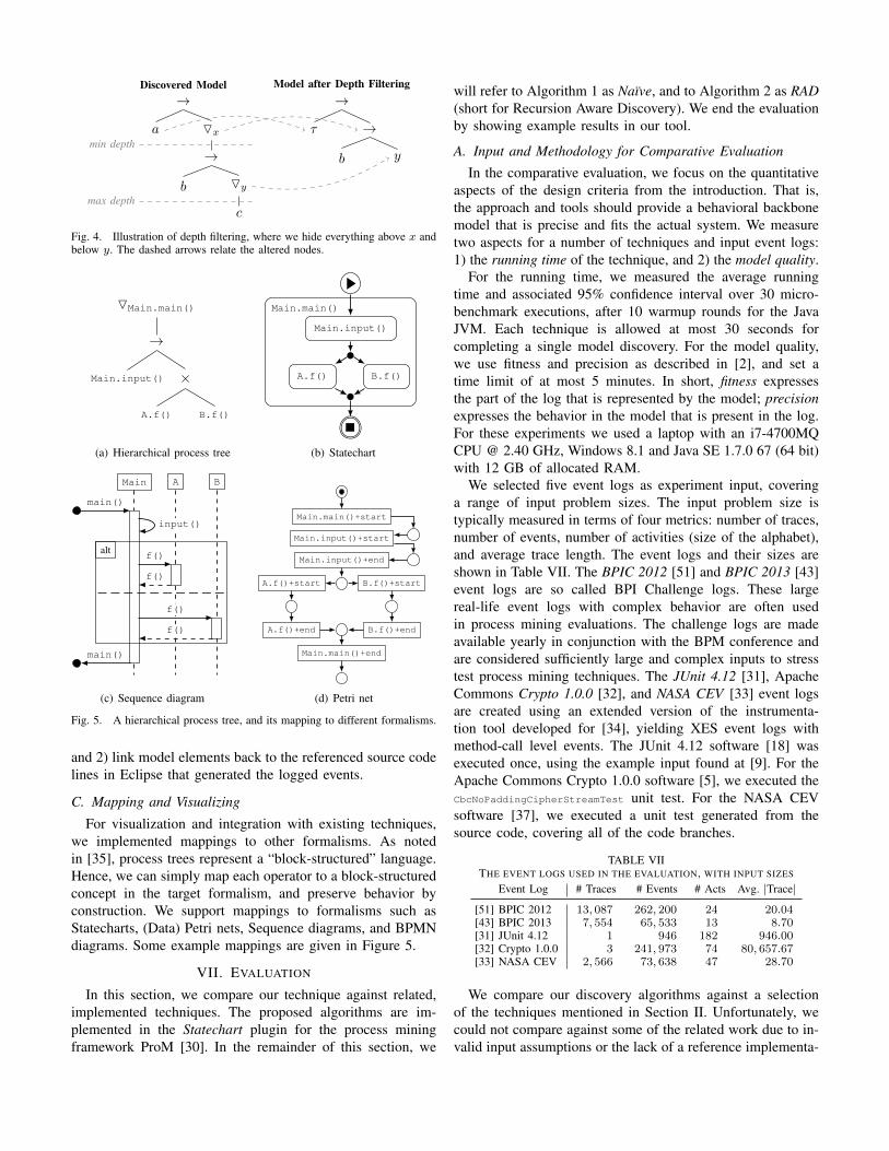
Based on hierarchical information, we allow both coarseand fine grained filtering. Using sliders, the user can quicklyselect a minimum and maximum hierarchical depth to inspect,and hide other parts of the model. The idea of depth filteringis illustrated in Figure 4. Afterwards, users can interactivelyfold and unfold parts of the hierarchy. By searching, userscan quickly locate areas of interest. Using term-based treerewriting (see Table VI), we present the user with a simplifiedmodel that preserves behavior.
TABLE VIREDUCTION RULES FOR (HIERARCHICAL) PROCESS TREES
⊗(P1) = P1 for ⊗ ∈ {→,×,∧}⊗(. . .1 ,⊗(. . .2), . . .3) = ⊗(. . .1 , . . .2 , . . .3) for ⊗ ∈ {→,∧}
⊗(. . .1 , τ, . . .2) = ⊗(. . .1 , . . .2) for ⊗ ∈ {→,∧}×(. . .1 , τ, . . .2) = ×(. . .1 , . . .2) if ε ∈ L(. . .1 ∪ . . .2)
B. Linking the Model to Event Data and the Source Code
For further analysis, like performance (timing), frequency(usage) and conformance, we annotate the discovered modelwith additional information. By annotating this informationonto (parts of) the model, we can visualize it in the context ofthe behavior. This annotation is based on the event log dataprovided as input and is partly provided by existing algorithmsin the Process Mining Toolkit ProM. Most notably, we 1) alignthe discovered model with the event log, as described in [2],
→
a Ox
→
b Oy
c
→
τ →
b y
Discovered Model Model after Depth Filtering
min depth
max depth
Fig. 4. Illustration of depth filtering, where we hide everything above x andbelow y. The dashed arrows relate the altered nodes.
OMain.main()
→
Main.input() ×
A.f() B.f()
(a) Hierarchical process tree
Main.input()
A.f() B.f()
Main.main()
(b) Statechart
Main A B
alt
main()
main()
input()
f()
f()
f()
f()
(c) Sequence diagram
Main.main()+start
Main.input()+start
Main.input()+end
A.f()+start
A.f()+end
B.f()+start
B.f()+end
Main.main()+end
(d) Petri net
Fig. 5. A hierarchical process tree, and its mapping to different formalisms.
and 2) link model elements back to the referenced source codelines in Eclipse that generated the logged events.
C. Mapping and Visualizing
For visualization and integration with existing techniques,we implemented mappings to other formalisms. As notedin [35], process trees represent a “block-structured” language.Hence, we can simply map each operator to a block-structuredconcept in the target formalism, and preserve behavior byconstruction. We support mappings to formalisms such asStatecharts, (Data) Petri nets, Sequence diagrams, and BPMNdiagrams. Some example mappings are given in Figure 5.
VII. EVALUATION
In this section, we compare our technique against related,implemented techniques. The proposed algorithms are im-plemented in the Statechart plugin for the process miningframework ProM [30]. In the remainder of this section, we
will refer to Algorithm 1 as Naıve, and to Algorithm 2 as RAD(short for Recursion Aware Discovery). We end the evaluationby showing example results in our tool.
A. Input and Methodology for Comparative Evaluation
In the comparative evaluation, we focus on the quantitativeaspects of the design criteria from the introduction. That is,the approach and tools should provide a behavioral backbonemodel that is precise and fits the actual system. We measuretwo aspects for a number of techniques and input event logs:1) the running time of the technique, and 2) the model quality.
For the running time, we measured the average runningtime and associated 95% confidence interval over 30 micro-benchmark executions, after 10 warmup rounds for the JavaJVM. Each technique is allowed at most 30 seconds forcompleting a single model discovery. For the model quality,we use fitness and precision as described in [2], and set atime limit of at most 5 minutes. In short, fitness expressesthe part of the log that is represented by the model; precisionexpresses the behavior in the model that is present in the log.For these experiments we used a laptop with an i7-4700MQCPU @ 2.40 GHz, Windows 8.1 and Java SE 1.7.0 67 (64 bit)with 12 GB of allocated RAM.
We selected five event logs as experiment input, coveringa range of input problem sizes. The input problem size istypically measured in terms of four metrics: number of traces,number of events, number of activities (size of the alphabet),and average trace length. The event logs and their sizes areshown in Table VII. The BPIC 2012 [51] and BPIC 2013 [43]event logs are so called BPI Challenge logs. These largereal-life event logs with complex behavior are often usedin process mining evaluations. The challenge logs are madeavailable yearly in conjunction with the BPM conference andare considered sufficiently large and complex inputs to stresstest process mining techniques. The JUnit 4.12 [31], ApacheCommons Crypto 1.0.0 [32], and NASA CEV [33] event logsare created using an extended version of the instrumenta-tion tool developed for [34], yielding XES event logs withmethod-call level events. The JUnit 4.12 software [18] wasexecuted once, using the example input found at [9]. For theApache Commons Crypto 1.0.0 software [5], we executed theCbcNoPaddingCipherStreamTest unit test. For the NASA CEVsoftware [37], we executed a unit test generated from thesource code, covering all of the code branches.
TABLE VIITHE EVENT LOGS USED IN THE EVALUATION, WITH INPUT SIZES
Event Log # Traces # Events # Acts Avg. |Trace|
[51] BPIC 2012 13, 087 262, 200 24 20.04[43] BPIC 2013 7, 554 65, 533 13 8.70[31] JUnit 4.12 1 946 182 946.00[32] Crypto 1.0.0 3 241, 973 74 80, 657.67[33] NASA CEV 2, 566 73, 638 47 28.70
We compare our discovery algorithms against a selectionof the techniques mentioned in Section II. Unfortunately, wecould not compare against some of the related work due to in-valid input assumptions or the lack of a reference implementa-
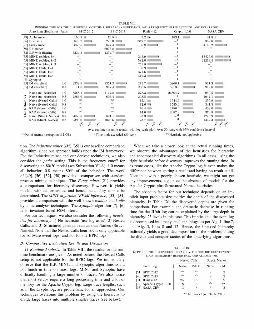
TABLE VIIIRUNNING TIME FOR THE DIFFERENT ALGORITHMS, HIERARCHY HEURISTICS, PATHS FREQUENCY FILTER SETTINGS, AND EVENT LOGS.
Algorithm (Heuristic) Paths BPIC 2012 BPIC 2013 JUnit 4.12 Crypto 1.0.0 NASA CEV
[49] Alpha miner 150.1
102
103
104
73.5
102
103
9.2
101
102
103
183.1
100
102
104
37.8
102
103
104
[56] Heuristics 840.2 278.0 1349.7 −T 359.6[21] Fuzzy miner 2858.5 827.4 166.8 −T 4148.2[50] ILP miner −T 6023.8 −T −T −T
[52] ILP with filtering 7234.3 4354.7 −T −T −T
[55] MINT, redblue, k=1 −T −T 243.9 −T 13426.0[55] MINT, redblue, k=2 −T −T 582.0 −T 22213.4[55] MINT, redblue, k=3 −T −T 751.8 −T −T
[55] MINT, ktails, k=1 −T −T 108.9 −T −T
[55] MINT, ktails, k=2 −T −T 371.6 −T −T
[55] MINT, ktails, k=3 −T −T 512.3 −T −T
[7] Synoptic −T −T −T −T −T
[35] IM (baseline) 1.0 3239.9 1351.2 215.7 10866.1 911.3[35] IM (baseline) 0.8 5111.6 947.4 268.5 5213.9 912.6
Our
tech
niqu
es
Naıve (no heuristic) 1.0 3588.1 1117.8 278.3 26804.7 959.5Naıve (no heuristic) 0.8 2865.6 603.4 298.5 −T 1047.1Naıve (Nested Calls) 1.0 n/a n/a 15.1 1544.6 355.9Naıve (Nested Calls) 0.8 n/a n/a 12.6 1545.6 341.5RAD (Nested Calls) 1.0 n/a n/a 16.4 2186.4 439.0RAD (Nested Calls) 0.8 n/a n/a 14.6 2082.8 373.8Naıve (Struct. Names) 0.8 2058.6 891.1 23.3 −M 1275.9RAD (Struct. Names) 0.8 2395.0 1028.6 23.7 −M 1452.3
Avg. runtime (in milliseconds, with log scale plot), over 30 runs, with 95% confidence intervalM Out of memory exception (12 GB) T Time limit exceeded (30 sec.) n/a Heuristic not applicable
tion. The Inductive miner (IM) [35] is our baseline comparisonalgorithm, since our approach builds upon the IM framework.For the Inductive miner and our derived techniques, we alsoconsider the paths setting. This is the frequency cutoff fordiscovering an 80/20 model (see Subsection VI-A): 1.0 meansall behavior, 0.8 means 80% of the behavior. The workof [49], [56], [52], [50] provides a comparison with standardprocess mining techniques. The Fuzzy miner [21] providesa comparison for hierarchy discovery. However, it yieldsmodels without semantics, and hence the quality cannot bedetermined. The MINT algorithm (EFSM inference) [55], [54]provides a comparison with the well-known redblue and ktailsdynamic analysis techniques. The Synoptic algorithm [7], [6]is an invariant based FSM inferrer.
For our techniques, we also consider the following heuris-tics for hierarchy: 1) No heuristic (use log as is), 2) NestedCalls, and 3) Structured package.class.method Names (Struct.Names). Note that the Nested Calls heuristic is only applicablefor software event logs, and not for the BPIC logs.
B. Comparative Evaluation Results and Discussion
1) Runtime Analysis: In Table VIII, the results for the run-time benchmark are given. As noted before, the Nested Callssetup is not applicable for the BPIC logs. We immediatelyobserve that the ILP, MINT, and Synoptic algorithms couldnot finish in time on most logs. MINT and Synoptic havedifficulty handling a large number of traces. We also noticethat most setups require a long processing time and a lot ofmemory for the Apache Crypto log. Large trace lengths, suchas in the Crypto log, are problematic for all approaches. Ourtechniques overcome this problem by using the hierarchy todivide large traces into multiple smaller traces (see below).
When we take a closer look at the actual running times,we observe the advantages of the heuristics for hierarchyand accompanied discovery algorithms. In all cases, using theright heuristic before discovery improves the running time. Inextreme cases, like the Apache Crypto log, it even makes thedifference between getting a result and having no result at all.Note that, with a poorly chosen heuristic, we might not getany improvements, e.g., note the absence of models for theApache Crypto plus Structured Names heuristics.
The speedup factor for our technique depends on an im-plicit input problem size metric: the depth of the discoveredhierarchy. In Table IX, the discovered depths are given forcomparison. For example, the dramatic decrease in runningtime for the JUnit log can be explained by the large depth inhierarchy: 25 levels in this case. This implies that the event logis decomposed into many smaller sublogs, as per Alg. 1, line 7,and Alg. 3, lines 8 and 12. Hence, the imposed hierarchyindirectly yields a good decomposition of the problem, aidingthe divide and conquer tactics of the underlying algorithms.
TABLE IXDEPTH OF THE DISCOVERED HIERARCHY, FOR THE DIFFERENT EVENT
LOGS, HIERARCHY HEURISTICS, AND ALGORITHMS
Nested Calls Struct. Names
Event Log Naıve RAD Naıve RAD
[51] BPIC 2012 n/a n/a 2 2[43] BPIC 2013 n/a n/a 2 2[31] JUnit 4.12 25 18 9 9[32] Apache Crypto 1.0.0 8 8 n/a n/a
[33] NASA CEV 3 3 3 3
n/a No model (see Table VIII)
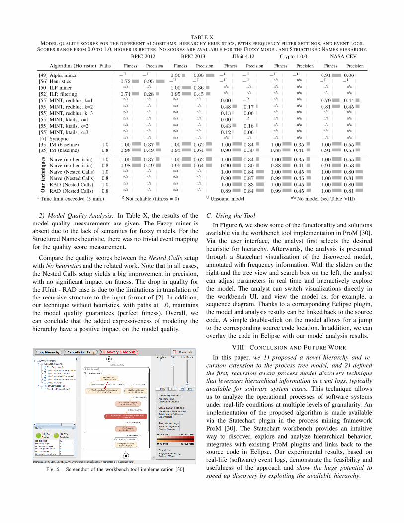
TABLE XMODEL QUALITY SCORES FOR THE DIFFERENT ALGORITHMS, HIERARCHY HEURISTICS, PATHS FREQUENCY FILTER SETTINGS, AND EVENT LOGS.
SCORES RANGE FROM 0.0 TO 1.0, HIGHER IS BETTER. NO SCORES ARE AVAILABLE FOR THE FUZZY MODEL AND STRUCTURED NAMES HIERARCHY.BPIC 2012 BPIC 2013 JUnit 4.12 Crypto 1.0.0 NASA CEV
Algorithm (Heuristic) Paths Fitness Precision Fitness Precision Fitness Precision Fitness Precision Fitness Precision
[49] Alpha miner −U −U 0.36 0.88 −U −U −U −U 0.91 0.06[56] Heuristics 0.72 0.95 −U −U −U −U n/a n/a −U −U
[50] ILP miner n/a n/a 1.00 0.36 n/a n/a n/a n/a n/a n/a
[52] ILP, filtering 0.74 0.28 0.95 0.45 n/a n/a n/a n/a n/a n/a
[55] MINT, redblue, k=1 n/a n/a n/a n/a 0.00 −R n/a n/a 0.79 0.44[55] MINT, redblue, k=2 n/a n/a n/a n/a 0.48 0.17 n/a n/a 0.81 0.45[55] MINT, redblue, k=3 n/a n/a n/a n/a 0.13 0.06 n/a n/a n/a n/a
[55] MINT, ktails, k=1 n/a n/a n/a n/a 0.00 −R n/a n/a n/a n/a
[55] MINT, ktails, k=2 n/a n/a n/a n/a 0.43 0.16 n/a n/a n/a n/a
[55] MINT, ktails, k=3 n/a n/a n/a n/a 0.12 0.06 n/a n/a n/a n/a
[7] Synoptic n/a n/a n/a n/a n/a n/a n/a n/a n/a n/a
[35] IM (baseline) 1.0 1.00 0.37 1.00 0.62 1.00 0.34 1.00 0.35 1.00 0.55[35] IM (baseline) 0.8 0.98 0.49 0.95 0.64 0.90 0.30 0.88 0.41 0.91 0.53
Our
tech
niqu
es Naıve (no heuristic) 1.0 1.00 0.37 1.00 0.62 1.00 0.34 1.00 0.35 1.00 0.55Naıve (no heuristic) 0.8 0.98 0.49 0.95 0.64 0.90 0.30 0.88 0.41 0.91 0.53Naıve (Nested Calls) 1.0 n/a n/a n/a n/a 1.00 0.84 1.00 0.45 1.00 0.80Naıve (Nested Calls) 0.8 n/a n/a n/a n/a 0.90 0.87 0.99 0.45 1.00 0.81RAD (Nested Calls) 1.0 n/a n/a n/a n/a 1.00 0.83 1.00 0.45 1.00 0.80RAD (Nested Calls) 0.8 n/a n/a n/a n/a 0.89 0.84 0.99 0.45 1.00 0.81
T Time limit exceeded (5 min.) R Not reliable (fitness = 0) U Unsound model n/a No model (see Table VIII)
2) Model Quality Analysis: In Table X, the results of themodel quality measurements are given. The Fuzzy miner isabsent due to the lack of semantics for fuzzy models. For theStructured Names heuristic, there was no trivial event mappingfor the quality score measurement.
Compare the quality scores between the Nested Calls setupwith No heuristics and the related work. Note that in all cases,the Nested Calls setup yields a big improvement in precision,with no significant impact on fitness. The drop in quality forthe JUnit - RAD case is due to the limitations in translation ofthe recursive structure to the input format of [2]. In addition,our technique without heuristics, with paths at 1.0, maintainsthe model quality guarantees (perfect fitness). Overall, wecan conclude that the added expressiveness of modeling thehierarchy have a positive impact on the model quality.
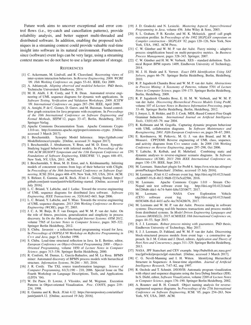
Fig. 6. Screenshot of the workbench tool implementation [30]
C. Using the Tool
In Figure 6, we show some of the functionality and solutionsavailable via the workbench tool implementation in ProM [30].Via the user interface, the analyst first selects the desiredheuristic for hierarchy. Afterwards, the analysis is presentedthrough a Statechart visualization of the discovered model,annotated with frequency information. With the sliders on theright and the tree view and search box on the left, the analystcan adjust parameters in real time and interactively explorethe model. The analyst can switch visualizations directly inthe workbench UI, and view the model as, for example, asequence diagram. Thanks to a corresponding Eclipse plugin,the model and analysis results can be linked back to the sourcecode. A simple double-click on the model allows for a jumpto the corresponding source code location. In addition, we canoverlay the code in Eclipse with our model analysis results.
VIII. CONCLUSION AND FUTURE WORK
In this paper, we 1) proposed a novel hierarchy and re-cursion extension to the process tree model; and 2) definedthe first, recursion aware process model discovery techniquethat leverages hierarchical information in event logs, typicallyavailable for software system cases. This technique allowsus to analyze the operational processes of software systemsunder real-life conditions at multiple levels of granularity. Animplementation of the proposed algorithm is made availablevia the Statechart plugin in the process mining frameworkProM [30]. The Statechart workbench provides an intuitiveway to discover, explore and analyze hierarchical behavior,integrates with existing ProM plugins and links back to thesource code in Eclipse. Our experimental results, based onreal-life (software) event logs, demonstrate the feasibility andusefulness of the approach and show the huge potential tospeed up discovery by exploiting the available hierarchy.
Future work aims to uncover exceptional and error con-trol flows (i.e., try-catch and cancellation patterns), providereliability analysis, and better support multi-threaded anddistributed software. In addition, enabling the proposed tech-niques in a streaming context could provide valuable real-timeinsight into software in its natural environment. Furthermore,since (software) event logs can be very large, using a streamingcontext means we do not have to use a large amount of storage.
REFERENCES
[1] C. Ackermann, M. Lindvall, and R. Cleaveland. Recovering views ofinter-system interaction behaviors. In Reverse Engineering, 2009. WCRE’09. 16th Working Conference on, pages 53–61. IEEE, Oct 2009.
[2] A. Adriansyah. Aligning observed and modeled behavior. PhD thesis,Technische Universiteit Eindhoven, 2014.
[3] M. H. Alalfi, J. R. Cordy, and T. R. Dean. Automated reverse engi-neering of UML sequence diagrams for dynamic web applications. InSoftware Testing, Verification and Validation Workshops, 2009. ICSTW’09. International Conference on, pages 287–294. IEEE, April 2009.
[4] A. Amighi, P. de C. Gomes, D. Gurov, and M. Huisman. Sound control-flow graph extraction for Java programs with exceptions. In Proceedingsof the 10th International Conference on Software Engineering andFormal Methods, SEFM’12, pages 33–47, Berlin, Heidelberg, 2012.Springer-Verlag.
[5] Apache Commons Documentation Team. Apache Commons Crypto1.0.0-src. http://commons.apache.org/proper/commons-crypto. [Online,accessed 3 March 2017].
[6] I. Beschastnikh. Synoptic Model Inference. https://github.com/ModelInference/synoptic. [Online, accessed 31 August 2017].
[7] I. Beschastnikh, J. Abrahamson, Y. Brun, and M. D. Ernst. Synoptic:Studying logged behavior with inferred models. In Proceedings of the19th ACM SIGSOFT Symposium and the 13th European Conference onFoundations of Software Engineering, ESEC/FSE ’11, pages 448–451,New York, NY, USA, 2011. ACM.
[8] I. Beschastnikh, Y. Brun, M. D. Ernst, and A. Krishnamurthy. Inferringmodels of concurrent systems from logs of their behavior with CSight.In Proceedings of the 36th International Conference on Software Engi-neering, ICSE 2014, pages 468–479, New York, NY, USA, 2014. ACM.
[9] S. Birkner, E. Gamma, and K. Beck. JUnit 4 - Getting Started. https://github.com/junit-team/junit4/wiki/Getting-started. [Online, accessed 19July 2016].
[10] L. C. Briand, Y. Labiche, and J. Leduc. Toward the reverse engineeringof UML sequence diagrams for distributed Java software. SoftwareEngineering, IEEE Transactions on, 32(9):642–663, Sept 2006.
[11] L. C. Briand, Y. Labiche, and Y. Miao. Towards the reverse engineeringof UML sequence diagrams. 2013 20th Working Conference on ReverseEngineering (WCRE), page 57, 2003.
[12] J. C. A. M. Buijs, B. F. van Dongen, and W. M. P. van der Aalst. Onthe role of fitness, precision, generalization and simplicity in processdiscovery. In On the Move to Meaningful Internet Systems: OTM 2012,volume 7565 of Lecture Notes in Computer Science, pages 305–322.Springer Berlin Heidelberg, 2012.
[13] S. Chiba. Javassist – a reflection-based programming wizard for Java.In Proceedings of OOPSLA’98 Workshop on Reflective Programming inC++ and Java, page 5, October 1998.
[14] S. Chiba. Load-time structural reflection in Java. In E. Bertino, editor,European Conference on Object-Oriented Programming 2000 – Object-Oriented Programming, volume 1850 of Lecture Notes in ComputerScience, pages 313–336. Springer Berlin Heidelberg, 2000.
[15] R. Conforti, M. Dumas, L. Garcıa-Banuelos, and M. La Rosa. BPMNminer: Automated discovery of BPMN process models with hierarchicalstructure. Information Systems, 56:284 – 303, 2016.
[16] J. R. Cordy. The TXL source transformation language. Science ofComputer Programming, 61(3):190 – 210, 2006. Special Issue on TheFourth Workshop on Language Descriptions, Tools, and Applications(LDTA ’04).
[17] W. De Pauw, D. Lorenz, J. Vlissides, and M. Wegman. ExecutionPatterns in Object-oriented Visualization. Proc. COOTS, pages 219–234, 1998.
[18] E. Gamma and K. Beck. JUnit 4.12. https://mvnrepository.com/artifact/junit/junit/4.12. [Online, accessed 19 July 2016].
[19] J. D. Gradecki and N. Lesiecki. Mastering AspectJ. Aspect-OrientedProgramming in Java, volume 456. John Wiley & Sons, 2003.
[20] S. L. Graham, P. B. Kessler, and M. K. Mckusick. gprof: call graphexecution profiler. In Proceedings of the 1982 SIGPLAN symposium onCompiler construction - SIGPLAN ’82, pages 120–126, New York, NewYork, USA, 1982. ACM Press.
[21] C. W. Gunther and W. M. P. van der Aalst. Fuzzy mining – adaptiveprocess simplification based on multi-perspective metrics. In BusinessProcess Management, pages 328–343. Springer, 2007.
[22] C. W. Gunther and H. M. W. Verbeek. XES – standard definition. Tech-nical Report BPM reports 1409, Eindhoven University of Technology,2014.
[23] M. J. H. Heule and S. Verwer. Exact DFA Identification Using SATSolvers, pages 66–79. Springer Berlin Heidelberg, Berlin, Heidelberg,2010.
[24] R. P. Jagadeesh Chandra Bose and W. M. P. van der Aalst. Abstractionsin Process Mining: A Taxonomy of Patterns, volume 5701 of LectureNotes in Computer Science, pages 159–175. Springer Berlin Heidelberg,Berlin, Heidelberg, 2009.
[25] R. P. Jagadeesh Chandra Bose, E. H. M. W. Verbeek, and W. M. P.van der Aalst. Discovering Hierarchical Process Models Using ProM,volume 107 of Lecture Notes in Business Information Processing, pages33–48. Springer Berlin Heidelberg, Berlin, Heidelberg, 2012.
[26] I. Jonyer, L. B. Holder, and D. J. Cook. MDL-Based Context-Free GraphGrammar Induction. International Journal on Artificial IntelligenceTools, 13(01):65–79, mar 2004.
[27] R. Kollmann and M. Gogolla. Capturing dynamic program behaviourwith UML collaboration diagrams. In Software Maintenance andReengineering, 2001. Fifth European Conference on, pages 58–67, 2001.
[28] E. Korshunova, M. Petkovic, M. G. J. van den Brand, and M. R.Mousavi. CPP2XMI: Reverse engineering of UML class, sequence,and activity diagrams from C++ source code. In 2006 13th WorkingConference on Reverse Engineering, pages 297–298, Oct 2006.
[29] Y. Labiche, B. Kolbah, and H. Mehrfard. Combining static anddynamic analyses to reverse-engineer scenario diagrams. In SoftwareMaintenance (ICSM), 2013 29th IEEE International Conference on,pages 130–139. IEEE, Sept 2013.
[30] M. Leemans. Statechart plugin for ProM 6. https://svn.win.tue.nl/repos/prom/Packages/Statechart/. [Online, accessed 15 July 2016].
[31] M. Leemans. JUnit 4.12 software event log. http://doi.org/10.4121/uuid:cfed8007-91c8-4b12-98d8-f233e5cd25bb, 2016.
[32] M. Leemans. Apache Commons Crypto 1.0.0 - Stream Cbc-Nopad unit test software event log. http://doi.org/10.4121/uuid:bb3286d6-dde1-4e74-9a64-fd4e32f10677, 2017.
[33] M. Leemans. NASA Crew Exploration Vehicle(CEV) software event log. http://doi.org/10.4121/uuid:60383406-ffcd-441f-aa5e-4ec763426b76, 2017.
[34] M. Leemans and W. M. P. van der Aalst. Process mining in softwaresystems: Discovering real-life business transactions and process modelsfrom distributed systems. In Model Driven Engineering Languages andSystems (MODELS), 2015 ACM/IEEE 18th International Conference on,pages 44–53, Sept 2015.
[35] S. J. J. Leemans. Robust process mining with guarantees. PhD thesis,Eindhoven University of Technology, May 2017.
[36] S. J. J. Leemans, D. Fahland, and W. M. P. van der Aalst. Discoveringblock-structured process models from event logs - a constructive ap-proach. In J. M. Colom and J. Desel, editors, Application and Theory ofPetri Nets and Concurrency, pages 311–329. Springer Berlin Heidelberg,2013.
[37] NASA. JPF Statechart and CEV example. http://babelfish.arc.nasa.gov/trac/jpf/wiki/projects/jpf-statechart. [Online, accessed 3 March 2017].
[38] C. G. Nevill-Manning and I. H. Witten. Identifying HierarchicalStructure in Sequences: A linear-time algorithm. Journal of ArtificialIntelligence Research, 7:67–82, aug 1997.
[39] R. Oechsle and T. Schmitt. JAVAVIS: Automatic program visualizationwith object and sequence diagrams using the Java Debug Interface (JDI).In S. Diehl, editor, Software Visualization, volume 2269 of Lecture Notesin Computer Science, pages 176–190. Springer Berlin Heidelberg, 2002.
[40] A. Rountev and B. H. Connell. Object naming analysis for reverse-engineered sequence diagrams. In Proceedings of the 27th InternationalConference on Software Engineering, ICSE ’05, pages 254–263, NewYork, NY, USA, 2005. ACM.
[41] P. Siyari, B. Dilkina, and C. Dovrolis. Lexis: An Optimization Frame-work for Discovering the Hierarchical Structure of Sequential Data.Gecco, pages 421–434, feb 2016.
[42] O. Spinczyk, A. Gal, and W. Schroder-Preikschat. AspectC++: Anaspect-oriented extension to the C++ programming language. In Pro-ceedings of the Fortieth International Conference on Tools Pacific: Ob-jects for Internet, Mobile and Embedded Applications, CRPIT ’02, pages53–60, Darlinghurst, Australia, Australia, 2002. Australian ComputerSociety, Inc.
[43] W. Steeman. BPI Challenge 2013, incidents. http://dx.doi.org/10.4121/uuid:500573e6-accc-4b0c-9576-aa5468b10cee, 2013.
[44] T. Systa, K. Koskimies, and H. Muller. Shimba – an environmentfor reverse engineering Java software systems. Software: Practice andExperience, 31(4):371–394, 2001.
[45] P. Tonella and A. Potrich. Reverse engineering of the interactiondiagrams from C++ code. In Software Maintenance, 2003. ICSM 2003.Proceedings. International Conference on, pages 159–168, Sept 2003.
[46] W. M. P. van der Aalst. Process Mining: Data Science in Action.Springer-Verlag, Berlin, 2016.
[47] W. M. P. van der Aalst, A. K. Alves de Medeiros, and A. J. M. M.Weijters. Genetic Process Mining. In G. Ciardo and P. Darondeau,editors, Applications and Theory of Petri Nets 2005, volume 3536of Lecture Notes in Computer Science, pages 48–69. Springer-Verlag,Berlin, 2005.
[48] W. M. P. van der Aalst, V. Rubin, H. M. W. Verbeek, B. F. van Dongen,E. Kindler, and C. W. Gunther. Process mining: a two-step approachto balance between underfitting and overfitting. Software & SystemsModeling, 9(1):87–111, 2010.
[49] W. M. P. van der Aalst, A. J. M. M. Weijters, and L. Maruster.Workflow Mining: Discovering Process Models from Event Logs. IEEETransactions on Knowledge and Data Engineering, 16(9):1128–1142,2004.
[50] J. M. E. M. van der Werf, B. F. van Dongen, C. A. J. Hurkens, andA. Serebrenik. Process Discovery Using Integer Linear Programming,pages 368–387. Springer Berlin Heidelberg, Berlin, Heidelberg, 2008.
[51] B.F. van Dongen. BPI Challenge 2012. http://dx.doi.org/10.4121/uuid:3926db30-f712-4394-aebc-75976070e91f, 2012.
[52] S. J. van Zelst, B. F. van Dongen, and W. M. P. van der Aalst. AvoidingOver-Fitting in ILP-Based Process Discovery, pages 163–171. SpringerInternational Publishing, Cham, 2015.
[53] H. M. W. Verbeek, J. C. A. M. Buijs, B. F. van Dongen, and W. M. P.van der Aalst. XES, XESame, and ProM 6. In P. Soffer andE. Proper, editors, Information Systems Evolution, volume 72 of LectureNotes in Business Information Processing, pages 60–75. Springer BerlinHeidelberg, 2011.
[54] N. Walkinshaw. EFSMInferenceTool. https://bitbucket.org/nwalkinshaw/efsminferencetool. [Online, accessed 19 July 2016].
[55] N. Walkinshaw, R. Taylor, and J. Derrick. Inferring extended finitestate machine models from software executions. Empirical SoftwareEngineering, 21(3):811–853, 2016.
[56] A. J. M. M. Weijters and J. T. S. Ribeiro. Flexible Heuristics Miner(FHM). In 2011 IEEE Symposium on Computational Intelligence andData Mining (CIDM), pages 310–317, April 2011.
[57] Z. Yao, Q. Zheng, and G. Chen. AOP++: A generic aspect-orientedprogramming framework in C++. In R. Gluck and M. Lowry, editors,Generative Programming and Component Engineering, volume 3676of Lecture Notes in Computer Science, pages 94–108. Springer BerlinHeidelberg, 2005.