Embed Size (px)
Citation preview
Recursion
CSE235
Introduction
RecurrenceRelations
LinearHomogeneousRecurrences
Non-homogenous
OtherMethods
Recursion
Slides by Christopher M. BourkeInstructor: Berthe Y. Choueiry
Fall 2007
Computer Science & Engineering 235Introduction to Discrete Mathematics
Sections 7.1 - 7.2 of [email protected] / 47
Recursion
CSE235
Introduction
RecurrenceRelations
LinearHomogeneousRecurrences
Non-homogenous
OtherMethods
Recursive Algorithms
A recursive algorithm is one in which objects are defined interms of other objects of the same type.
Advantages:
Simplicity of code
Easy to understand
Disadvantages:
Memory
Speed
Possibly redundant work
Tail recursion offers a solution to the memory problem, butreally, do we need recursion?
2 / 47
Recursion
CSE235
Introduction
RecurrenceRelations
LinearHomogeneousRecurrences
Non-homogenous
OtherMethods
Recursive AlgorithmsAnalysis
We’ve already seen how to analyze the running time ofalgorithms. However, to analyze recursive algorithms, werequire more sophisticated techniques.
Specifically, we study how to define & solve recurrencerelations.
3 / 47
Recursion
CSE235
Introduction
RecurrenceRelations
LinearHomogeneousRecurrences
Non-homogenous
OtherMethods
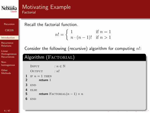
Motivating ExampleFactorial
Recall the factorial function.
n! ={
1 if n = 1n · (n− 1)! if n > 1
Consider the following (recursive) algorithm for computing n!:
Algorithm (Factorial)
Input : n ∈ NOutput : n!
if n = 1 then1return 12
end3
else4return Factorial(n− 1)× n5
end6
4 / 47
Recursion
CSE235
Introduction
RecurrenceRelations
LinearHomogeneousRecurrences
Non-homogenous
OtherMethods
Motivating ExampleFactorial - Analysis?
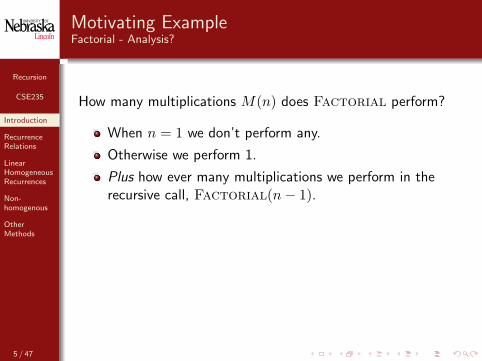
How many multiplications M(n) does Factorial perform?
When n = 1 we don’t perform any.
Otherwise we perform 1.
Plus how ever many multiplications we perform in therecursive call, Factorial(n− 1).This can be expressed as a formula (similar to thedefinition of n!.
M(0) = 0M(n) = 1 + M(n− 1)
This is known as a recurrence relation.
5 / 47

Recursion
CSE235
Introduction
RecurrenceRelations
LinearHomogeneousRecurrences
Non-homogenous
OtherMethods
Motivating ExampleFactorial - Analysis?
How many multiplications M(n) does Factorial perform?
When n = 1 we don’t perform any.
Otherwise we perform 1.
Plus how ever many multiplications we perform in therecursive call, Factorial(n− 1).This can be expressed as a formula (similar to thedefinition of n!.
M(0) = 0M(n) = 1 + M(n− 1)
This is known as a recurrence relation.
5 / 47
Recursion
CSE235
Introduction
RecurrenceRelations
LinearHomogeneousRecurrences
Non-homogenous
OtherMethods
Motivating ExampleFactorial - Analysis?
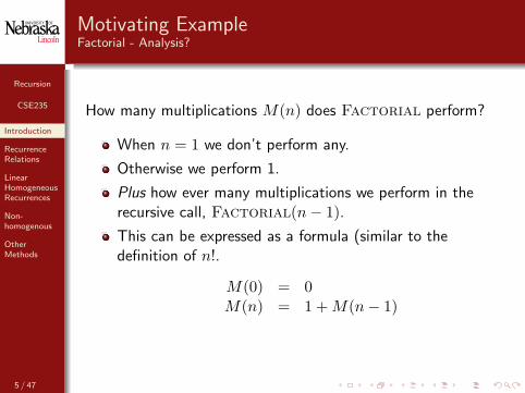
How many multiplications M(n) does Factorial perform?
When n = 1 we don’t perform any.
Otherwise we perform 1.
Plus how ever many multiplications we perform in therecursive call, Factorial(n− 1).
This can be expressed as a formula (similar to thedefinition of n!.
M(0) = 0M(n) = 1 + M(n− 1)
This is known as a recurrence relation.
5 / 47
Recursion
CSE235
Introduction
RecurrenceRelations
LinearHomogeneousRecurrences
Non-homogenous
OtherMethods
Motivating ExampleFactorial - Analysis?
How many multiplications M(n) does Factorial perform?
When n = 1 we don’t perform any.
Otherwise we perform 1.
Plus how ever many multiplications we perform in therecursive call, Factorial(n− 1).This can be expressed as a formula (similar to thedefinition of n!.
M(0) = 0M(n) = 1 + M(n− 1)
This is known as a recurrence relation.
5 / 47
Recursion
CSE235
Introduction
RecurrenceRelations
LinearHomogeneousRecurrences
Non-homogenous
OtherMethods
Motivating ExampleFactorial - Analysis?
How many multiplications M(n) does Factorial perform?
When n = 1 we don’t perform any.
Otherwise we perform 1.
Plus how ever many multiplications we perform in therecursive call, Factorial(n− 1).This can be expressed as a formula (similar to thedefinition of n!.
M(0) = 0M(n) = 1 + M(n− 1)
This is known as a recurrence relation.
5 / 47
Recursion
CSE235
Introduction
RecurrenceRelations
LinearHomogeneousRecurrences
Non-homogenous
OtherMethods
Recurrence Relations IDefinition
Definition
A recurrence relation for a sequence {an} is an equation thatexpresses an in terms of one or more of the previous terms inthe sequence,
a0, a1, . . . , an−1
for all integers n ≥ n0 where n0 is a nonnegative integer.A sequence is called a solution of a recurrence relation if itsterms satisfy the recurrence relation.
6 / 47
Recursion
CSE235
Introduction
RecurrenceRelations
LinearHomogeneousRecurrences
Non-homogenous
OtherMethods
Recurrence Relations IIDefinition
Consider the recurrence relation: an = 2an−1 − an−2.It has the following sequences an as solutions:
1 an = 3n,
2 an = n + 1, and
3 an = 5.
Initial conditions + recurrence relation uniquely determine thesequence.
7 / 47
Recursion
CSE235
Introduction
RecurrenceRelations
LinearHomogeneousRecurrences
Non-homogenous
OtherMethods
Recurrence Relations IIIDefinition
Example
The Fibonacci numbers are defined by the recurrence,
F (n) = F (n− 1) + F (n− 2)F (1) = 1F (0) = 1
The solution to the Fibonacci recurrence is
fn =1√5
(1 +
√5
2
)n
− 1√5
(1−
√5
2
)n
(your book derives this solution).
8 / 47

Recursion
CSE235
Introduction
RecurrenceRelations
LinearHomogeneousRecurrences
Non-homogenous
OtherMethods
Recurrence Relations IVDefinition
More generally, recurrences can have the form
T (n) = αT (n− β) + f(n), T (δ) = c
or
T (n) = αT
(n
β
)+ f(n), T (δ) = c
Note that it may be necessary to define several T (δ), initialconditions.
9 / 47

Recursion
CSE235
Introduction
RecurrenceRelations
LinearHomogeneousRecurrences
Non-homogenous
OtherMethods
Recurrence Relations VDefinition
The initial conditions specify the value of the first fewnecessary terms in the sequence. In the Fibonacci numbers weneeded two initial conditions, F (0) = F (1) = 1 since F (n) wasdefined by the two previous terms in the sequence.
Initial conditions are also known as boundary conditions (asopposed to the general conditions).
From now on, we will use the subscript notation, so theFibonacci numbers are
fn = fn−1 + fn−2
f1 = 1f0 = 1
10 / 47
Recursion
CSE235
Introduction
RecurrenceRelations
LinearHomogeneousRecurrences
Non-homogenous
OtherMethods
Recurrence Relations VIDefinition
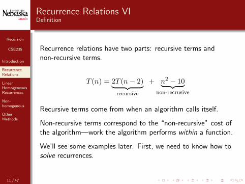
Recurrence relations have two parts: recursive terms andnon-recursive terms.
T (n) = 2T (n− 2)︸ ︷︷ ︸recursive
+ n2 − 10︸ ︷︷ ︸non-recrusive
Recursive terms come from when an algorithm calls itself.
Non-recursive terms correspond to the “non-recursive” cost ofthe algorithm—work the algorithm performs within a function.
We’ll see some examples later. First, we need to know how tosolve recurrences.
11 / 47
Recursion
CSE235
Introduction
RecurrenceRelations
LinearHomogeneousRecurrences
2nd Order
General
Non-homogenous
OtherMethods
Solving Recurrences
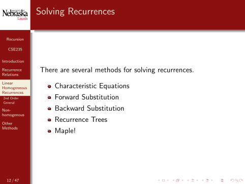
There are several methods for solving recurrences.
Characteristic Equations
Forward Substitution
Backward Substitution
Recurrence Trees
Maple!
12 / 47
Recursion
CSE235
Introduction
RecurrenceRelations
LinearHomogeneousRecurrences
2nd Order
General
Non-homogenous
OtherMethods
Linear Homogeneous Recurrences
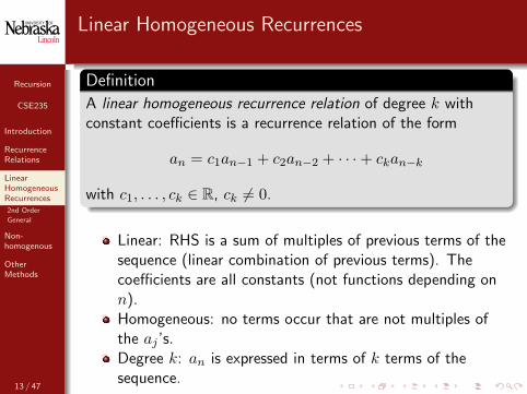
Definition
A linear homogeneous recurrence relation of degree k withconstant coefficients is a recurrence relation of the form
an = c1an−1 + c2an−2 + · · ·+ ckan−k
with c1, . . . , ck ∈ R, ck 6= 0.
Linear: RHS is a sum of multiples of previous terms of thesequence (linear combination of previous terms). Thecoefficients are all constants (not functions depending onn).Homogeneous: no terms occur that are not multiples ofthe aj ’s.Degree k: an is expressed in terms of k terms of thesequence.
13 / 47
Recursion
CSE235
Introduction
RecurrenceRelations
LinearHomogeneousRecurrences
2nd Order
General
Non-homogenous
OtherMethods
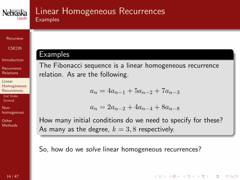
Linear Homogeneous RecurrencesExamples
Examples
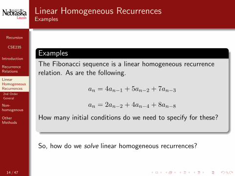
The Fibonacci sequence is a linear homogeneous recurrencerelation. As are the following.
an = 4an−1 + 5an−2 + 7an−3
an = 2an−2 + 4an−4 + 8an−8
How many initial conditions do we need to specify for these?
As many as the degree, k = 3, 8 respectively.
So, how do we solve linear homogeneous recurrences?
14 / 47
Recursion
CSE235
Introduction
RecurrenceRelations
LinearHomogeneousRecurrences
2nd Order
General
Non-homogenous
OtherMethods
Linear Homogeneous RecurrencesExamples
Examples
The Fibonacci sequence is a linear homogeneous recurrencerelation. As are the following.
an = 4an−1 + 5an−2 + 7an−3
an = 2an−2 + 4an−4 + 8an−8
How many initial conditions do we need to specify for these?As many as the degree, k = 3, 8 respectively.
So, how do we solve linear homogeneous recurrences?
14 / 47
Recursion
CSE235
Introduction
RecurrenceRelations
LinearHomogeneousRecurrences
2nd Order
General
Non-homogenous
OtherMethods
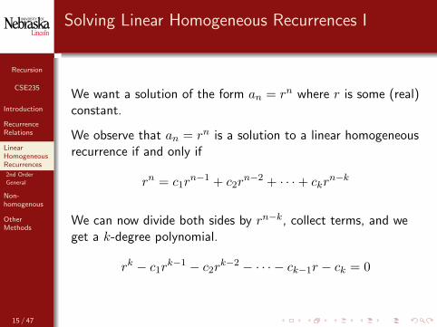
Solving Linear Homogeneous Recurrences I
We want a solution of the form an = rn where r is some (real)constant.
We observe that an = rn is a solution to a linear homogeneousrecurrence if and only if
rn = c1rn−1 + c2r
n−2 + · · ·+ ckrn−k
We can now divide both sides by rn−k, collect terms, and weget a k-degree polynomial.
rk − c1rk−1 − c2r
k−2 − · · · − ck−1r − ck = 0
15 / 47

Recursion
CSE235
Introduction
RecurrenceRelations
LinearHomogeneousRecurrences
2nd Order
General
Non-homogenous
OtherMethods
Solving Linear Homogeneous Recurrences II
rk − c1rk−1 − c2r
k−2 − · · · − ck−1r − ck = 0
This is called the characteristic equation of the recurrencerelation.
The roots of this polynomial are called the characteristic rootsof the recurrence relation. They can be used to find solutions(if they exist) to the recurrence relation. We will considerseveral cases.
16 / 47
Recursion
CSE235
Introduction
RecurrenceRelations
LinearHomogeneousRecurrences
2nd Order
General
Non-homogenous
OtherMethods
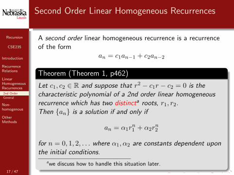
Second Order Linear Homogeneous Recurrences
A second order linear homogeneous recurrence is a recurrenceof the form
an = c1an−1 + c2an−2
Theorem (Theorem 1, p462)
Let c1, c2 ∈ R and suppose that r2 − c1r − c2 = 0 is thecharacteristic polynomial of a 2nd order linear homogeneousrecurrence which has two distincta roots, r1, r2.Then {an} is a solution if and only if
an = α1rn1 + α2r
n2
for n = 0, 1, 2, . . . where α1, α2 are constants dependent uponthe initial conditions.
awe discuss how to handle this situation later.17 / 47
Recursion
CSE235
Introduction
RecurrenceRelations
LinearHomogeneousRecurrences
2nd Order
General
Non-homogenous
OtherMethods
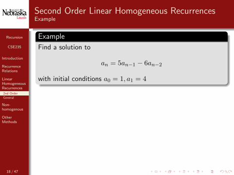
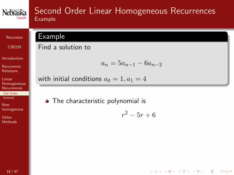
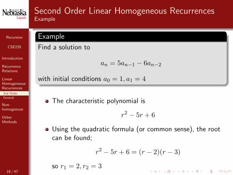
Second Order Linear Homogeneous RecurrencesExample
Example
Find a solution to
an = 5an−1 − 6an−2
with initial conditions a0 = 1, a1 = 4
The characteristic polynomial is
r2 − 5r + 6
Using the quadratic formula (or common sense), the rootcan be found;
r2 − 5r + 6 = (r − 2)(r − 3)
so r1 = 2, r2 = 3
18 / 47
Recursion
CSE235
Introduction
RecurrenceRelations
LinearHomogeneousRecurrences
2nd Order
General
Non-homogenous
OtherMethods
Second Order Linear Homogeneous RecurrencesExample
Example
Find a solution to
an = 5an−1 − 6an−2
with initial conditions a0 = 1, a1 = 4
The characteristic polynomial is
r2 − 5r + 6
Using the quadratic formula (or common sense), the rootcan be found;
r2 − 5r + 6 = (r − 2)(r − 3)
so r1 = 2, r2 = 318 / 47
Recursion
CSE235
Introduction
RecurrenceRelations
LinearHomogeneousRecurrences
2nd Order
General
Non-homogenous
OtherMethods
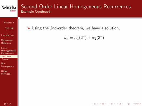
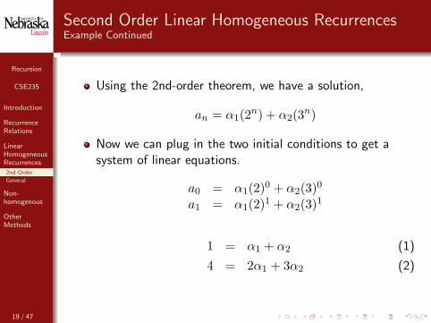
Second Order Linear Homogeneous RecurrencesExample Continued
Using the 2nd-order theorem, we have a solution,
an = α1(2n) + α2(3n)
Now we can plug in the two initial conditions to get asystem of linear equations.
a0 = α1(2)0 + α2(3)0
a1 = α1(2)1 + α2(3)1
1 = α1 + α2 (1)
4 = 2α1 + 3α2 (2)
19 / 47
Recursion
CSE235
Introduction
RecurrenceRelations
LinearHomogeneousRecurrences
2nd Order
General
Non-homogenous
OtherMethods
Second Order Linear Homogeneous RecurrencesExample Continued
Using the 2nd-order theorem, we have a solution,
an = α1(2n) + α2(3n)
Now we can plug in the two initial conditions to get asystem of linear equations.
a0 = α1(2)0 + α2(3)0
a1 = α1(2)1 + α2(3)1
1 = α1 + α2 (1)
4 = 2α1 + 3α2 (2)
19 / 47

Recursion
CSE235
Introduction
RecurrenceRelations
LinearHomogeneousRecurrences
2nd Order
General
Non-homogenous
OtherMethods
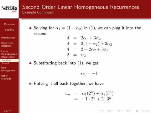
Second Order Linear Homogeneous RecurrencesExample Continued
Solving for α1 = (1− α2) in (1), we can plug it into thesecond.
4 = 2α1 + 3α2
4 = 2(1− α2) + 3α2
4 = 2− 2α2 + 3α2
2 = α2
Substituting back into (1), we get
α1 = −1
Putting it all back together, we have
an = α1(2n) + α2(3n)= −1 · 2n + 2 · 3n
20 / 47

Recursion
CSE235
Introduction
RecurrenceRelations
LinearHomogeneousRecurrences
2nd Order
General
Non-homogenous
OtherMethods
Second Order Linear Homogeneous RecurrencesExample Continued
Solving for α1 = (1− α2) in (1), we can plug it into thesecond.
4 = 2α1 + 3α2
4 = 2(1− α2) + 3α2
4 = 2− 2α2 + 3α2
2 = α2
Substituting back into (1), we get
α1 = −1
Putting it all back together, we have
an = α1(2n) + α2(3n)= −1 · 2n + 2 · 3n
20 / 47
Recursion
CSE235
Introduction
RecurrenceRelations
LinearHomogeneousRecurrences
2nd Order
General
Non-homogenous
OtherMethods
Second Order Linear Homogeneous RecurrencesAnother Example
Example
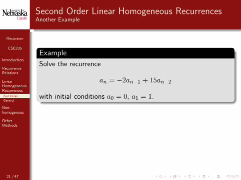
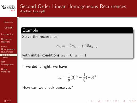
Solve the recurrence
an = −2an−1 + 15an−2
with initial conditions a0 = 0, a1 = 1.
If we did it right, we have
an =18(3)n − 1
8(−5)n
How can we check ourselves?
21 / 47
Recursion
CSE235
Introduction
RecurrenceRelations
LinearHomogeneousRecurrences
2nd Order
General
Non-homogenous
OtherMethods
Second Order Linear Homogeneous RecurrencesAnother Example
Example
Solve the recurrence
an = −2an−1 + 15an−2
with initial conditions a0 = 0, a1 = 1.
If we did it right, we have
an =18(3)n − 1
8(−5)n
How can we check ourselves?
21 / 47
Recursion
CSE235
Introduction
RecurrenceRelations
LinearHomogeneousRecurrences
2nd Order
General
Non-homogenous
OtherMethods
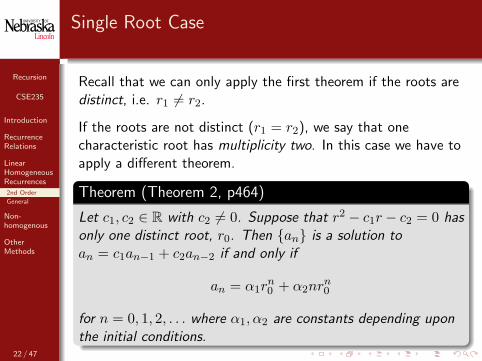
Single Root Case
Recall that we can only apply the first theorem if the roots aredistinct, i.e. r1 6= r2.
If the roots are not distinct (r1 = r2), we say that onecharacteristic root has multiplicity two. In this case we have toapply a different theorem.
Theorem (Theorem 2, p464)
Let c1, c2 ∈ R with c2 6= 0. Suppose that r2 − c1r − c2 = 0 hasonly one distinct root, r0. Then {an} is a solution toan = c1an−1 + c2an−2 if and only if
an = α1rn0 + α2nrn
0
for n = 0, 1, 2, . . . where α1, α2 are constants depending uponthe initial conditions.
22 / 47
Recursion
CSE235
Introduction
RecurrenceRelations
LinearHomogeneousRecurrences
2nd Order
General
Non-homogenous
OtherMethods
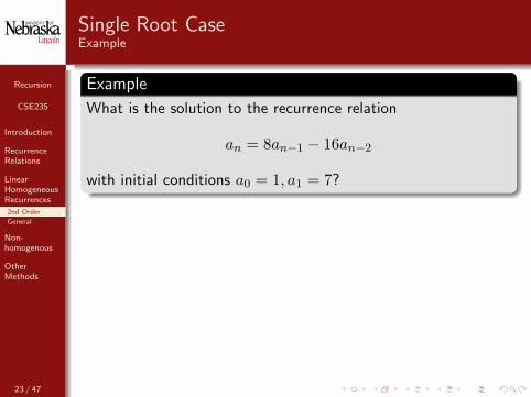
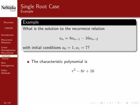
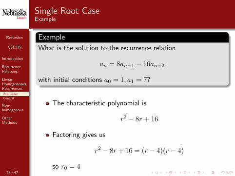
Single Root CaseExample
Example
What is the solution to the recurrence relation
an = 8an−1 − 16an−2
with initial conditions a0 = 1, a1 = 7?
The characteristic polynomial is
r2 − 8r + 16
Factoring gives us
r2 − 8r + 16 = (r − 4)(r − 4)
so r0 = 4
23 / 47
Recursion
CSE235
Introduction
RecurrenceRelations
LinearHomogeneousRecurrences
2nd Order
General
Non-homogenous
OtherMethods
Single Root CaseExample
Example
What is the solution to the recurrence relation
an = 8an−1 − 16an−2
with initial conditions a0 = 1, a1 = 7?
The characteristic polynomial is
r2 − 8r + 16
Factoring gives us
r2 − 8r + 16 = (r − 4)(r − 4)
so r0 = 423 / 47
Recursion
CSE235
Introduction
RecurrenceRelations
LinearHomogeneousRecurrences
2nd Order
General
Non-homogenous
OtherMethods
Single Root CaseExample
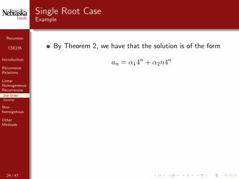
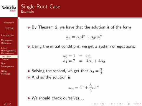
By Theorem 2, we have that the solution is of the form
an = α14n + α2n4n
Using the initial conditions, we get a system of equations;
a0 = 1 = α1
a1 = 7 = 4α1 + 4α2
Solving the second, we get that α2 = 34
And so the solution is
an = 4n +34n4n
We should check ourselves. . .
24 / 47

Recursion
CSE235
Introduction
RecurrenceRelations
LinearHomogeneousRecurrences
2nd Order
General
Non-homogenous
OtherMethods
Single Root CaseExample
By Theorem 2, we have that the solution is of the form
an = α14n + α2n4n
Using the initial conditions, we get a system of equations;
a0 = 1 = α1
a1 = 7 = 4α1 + 4α2
Solving the second, we get that α2 = 34
And so the solution is
an = 4n +34n4n
We should check ourselves. . .
24 / 47
Recursion
CSE235
Introduction
RecurrenceRelations
LinearHomogeneousRecurrences
2nd Order
General
Non-homogenous
OtherMethods
Single Root CaseExample
By Theorem 2, we have that the solution is of the form
an = α14n + α2n4n
Using the initial conditions, we get a system of equations;
a0 = 1 = α1
a1 = 7 = 4α1 + 4α2
Solving the second, we get that α2 = 34
And so the solution is
an = 4n +34n4n
We should check ourselves. . .24 / 47
Recursion
CSE235
Introduction
RecurrenceRelations
LinearHomogeneousRecurrences
2nd Order
General
Non-homogenous
OtherMethods
General Linear Homogeneous Recurrences
There is a straightforward generalization of these cases tohigher order linear homogeneous recurrences.
Essentially, we simply define higher degree polynomials.
The roots of these polynomials lead to a general solution.
The general solution contains coefficients that depend only onthe initial conditions.
In the general case, however, the coefficients form a system oflinear equalities.
25 / 47
Recursion
CSE235
Introduction
RecurrenceRelations
LinearHomogeneousRecurrences
2nd Order
General
Non-homogenous
OtherMethods
General Linear Homogeneous Recurrences IDistinct Roots
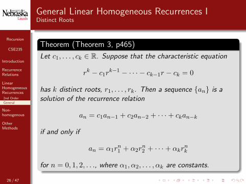
Theorem (Theorem 3, p465)
Let c1, . . . , ck ∈ R. Suppose that the characteristic equation
rk − c1rk−1 − · · · − ck−1r − ck = 0
has k distinct roots, r1, . . . , rk. Then a sequence {an} is asolution of the recurrence relation
an = c1an−1 + c2an−2 + · · ·+ ckan−k
if and only if
an = α1rn1 + α2r
n2 + · · ·+ αkr
nk
for n = 0, 1, 2, . . ., where α1, α2, . . . , αk are constants.
26 / 47
Recursion
CSE235
Introduction
RecurrenceRelations
LinearHomogeneousRecurrences
2nd Order
General
Non-homogenous
OtherMethods
General Linear Homogeneous RecurrencesAny Multiplicity
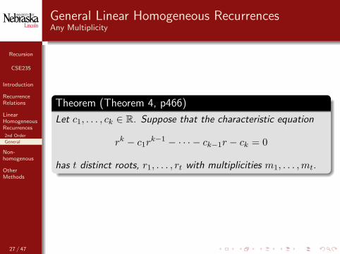
Theorem (Theorem 4, p466)
Let c1, . . . , ck ∈ R. Suppose that the characteristic equation
rk − c1rk−1 − · · · − ck−1r − ck = 0
has t distinct roots, r1, . . . , rt with multiplicities m1, . . . ,mt.
27 / 47
Recursion
CSE235
Introduction
RecurrenceRelations
LinearHomogeneousRecurrences
2nd Order
General
Non-homogenous
OtherMethods
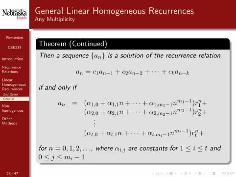
General Linear Homogeneous RecurrencesAny Multiplicity
Theorem (Continued)
Then a sequence {an} is a solution of the recurrence relation
an = c1an−1 + c2an−2 + · · ·+ ckan−k
if and only if
an = (α1,0 + α1,1n + · · ·+ α1,m1−1nm1−1)rn
1 +(α2,0 + α2,1n + · · ·+ α2,m2−1n
m2−1)rn2 +
...(αt,0 + αt,1n + · · ·+ αt,mt−1n
mt−1)rnt +
for n = 0, 1, 2, . . ., where αi,j are constants for 1 ≤ i ≤ t and0 ≤ j ≤ mi − 1.
28 / 47
Recursion
CSE235
Introduction
RecurrenceRelations
LinearHomogeneousRecurrences
Non-homogenous
OtherMethods
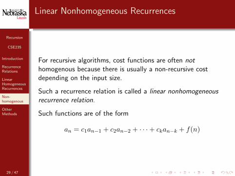
Linear Nonhomogeneous Recurrences
For recursive algorithms, cost functions are often nothomogenous because there is usually a non-recursive costdepending on the input size.
Such a recurrence relation is called a linear nonhomogeneousrecurrence relation.
Such functions are of the form
an = c1an−1 + c2an−2 + · · ·+ ckan−k + f(n)
29 / 47
Recursion
CSE235
Introduction
RecurrenceRelations
LinearHomogeneousRecurrences
Non-homogenous
OtherMethods
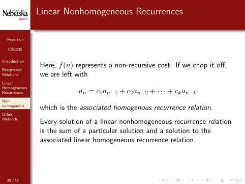
Linear Nonhomogeneous Recurrences
Here, f(n) represents a non-recursive cost. If we chop it off,we are left with
an = c1an−1 + c2an−2 + · · ·+ ckan−k
which is the associated homogenous recurrence relation.
Every solution of a linear nonhomogeneous recurrence relationis the sum of a particular solution and a solution to theassociated linear homogeneous recurrence relation.
30 / 47
Recursion
CSE235
Introduction
RecurrenceRelations
LinearHomogeneousRecurrences
Non-homogenous
OtherMethods
Linear Nonhomogeneous Recurrences
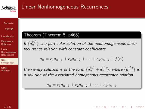
Theorem (Theorem 5, p468)
If {a(p)n } is a particular solution of the nonhomogeneous linear
recurrence relation with constant coefficients
an = c1an−1 + c2an−2 + · · ·+ ckan−k + f(n)
then every solution is of the form {a(p)n + a
(h)n }, where {a(h)
n } isa solution of the associated homogenous recurrence relation
an = c1an−1 + c2an−2 + · · ·+ ckan−k
31 / 47
Recursion
CSE235
Introduction
RecurrenceRelations
LinearHomogeneousRecurrences
Non-homogenous
OtherMethods
Linear Nonhomogeneous Recurrences
There is no general method for solving such relations.However, we can solve them for special cases.
In particular, if f(n) is a polynomial or exponential function (ormore precisely, when f(n) is the product of a polynomial andexponential function), then there is a general solution.
32 / 47
Recursion
CSE235
Introduction
RecurrenceRelations
LinearHomogeneousRecurrences
Non-homogenous
OtherMethods
Linear Nonhomogeneous Recurrences
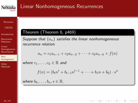
Theorem (Theorem 6, p469)
Suppose that {an} satisfies the linear nonhomogeneousrecurrence relation
an = c1an−1 + c2an−2 + · · ·+ ckan−k + f(n)
where c1, . . . , ck ∈ R and
f(n) = (btnt + bt−1n
t−1 + · · ·+ b1n + b0) · sn
where b0, . . . , bn, s ∈ R.
33 / 47
Recursion
CSE235
Introduction
RecurrenceRelations
LinearHomogeneousRecurrences
Non-homogenous
OtherMethods
Linear Nonhomogeneous Recurrences
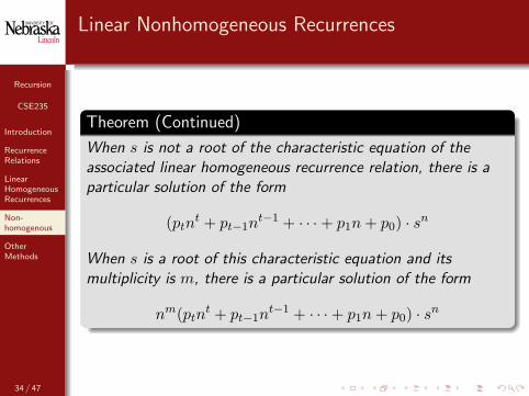
Theorem (Continued)
When s is not a root of the characteristic equation of theassociated linear homogeneous recurrence relation, there is aparticular solution of the form
(ptnt + pt−1n
t−1 + · · ·+ p1n + p0) · sn
When s is a root of this characteristic equation and itsmultiplicity is m, there is a particular solution of the form
nm(ptnt + pt−1n
t−1 + · · ·+ p1n + p0) · sn
34 / 47
Recursion
CSE235
Introduction
RecurrenceRelations
LinearHomogeneousRecurrences
Non-homogenous
OtherMethods
Linear Nonhomogeneous Recurrences
The examples in the text are quite good (see pp467–470) andillustrate how to solve simple nonhomogeneous relations.
We may go over more examples if you wish.
Also read up on generating functions in section 7.4 (though wemay return to this subject).
However, there are alternate, more intuitive methods.
35 / 47
Recursion
CSE235
Introduction
RecurrenceRelations
LinearHomogeneousRecurrences
Non-homogenous
OtherMethods
BackSubstitution
Recurrence Trees
Maple
Other Methods
When analyzing algorithms, linear homogenous recurrences oforder greater than 2 hardly ever arise in practice.
We briefly describe two “unfolding” methods that work for alot of cases.
Backward substitution – this works exactly as its nameimplies: starting from the equation itself, work backwards,substituting values of the function for previous ones.
Recurrence Trees – just as powerful but perhaps moreintuitive, this method involves mapping out the recurrence treefor an equation. Starting from the equation, you unfold eachrecursive call to the function and calculate the non-recursivecost at each level of the tree. You then find a general formulafor each level and take a summation over all such levels.
36 / 47
Recursion
CSE235
Introduction
RecurrenceRelations
LinearHomogeneousRecurrences
Non-homogenous
OtherMethods
BackSubstitution
Recurrence Trees
Maple
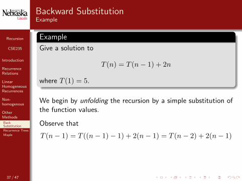
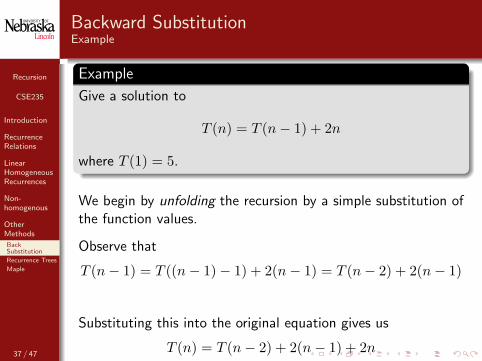
Backward SubstitutionExample
Example
Give a solution to
T (n) = T (n− 1) + 2n
where T (1) = 5.
We begin by unfolding the recursion by a simple substitution ofthe function values.
Observe that
T (n− 1) = T ((n− 1)− 1) + 2(n− 1) = T (n− 2) + 2(n− 1)
Substituting this into the original equation gives us
T (n) = T (n− 2) + 2(n− 1) + 2n
37 / 47
Recursion
CSE235
Introduction
RecurrenceRelations
LinearHomogeneousRecurrences
Non-homogenous
OtherMethods
BackSubstitution
Recurrence Trees
Maple
Backward SubstitutionExample
Example
Give a solution to
T (n) = T (n− 1) + 2n
where T (1) = 5.
We begin by unfolding the recursion by a simple substitution ofthe function values.
Observe that
T (n− 1) = T ((n− 1)− 1) + 2(n− 1) = T (n− 2) + 2(n− 1)
Substituting this into the original equation gives us
T (n) = T (n− 2) + 2(n− 1) + 2n37 / 47
Recursion
CSE235
Introduction
RecurrenceRelations
LinearHomogeneousRecurrences
Non-homogenous
OtherMethods
BackSubstitution
Recurrence Trees
Maple
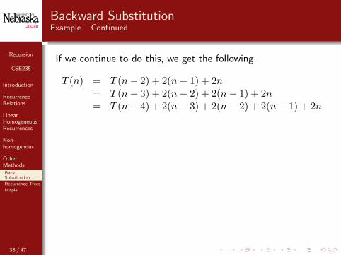
Backward SubstitutionExample – Continued
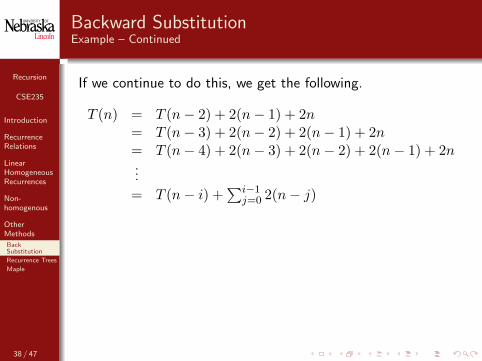
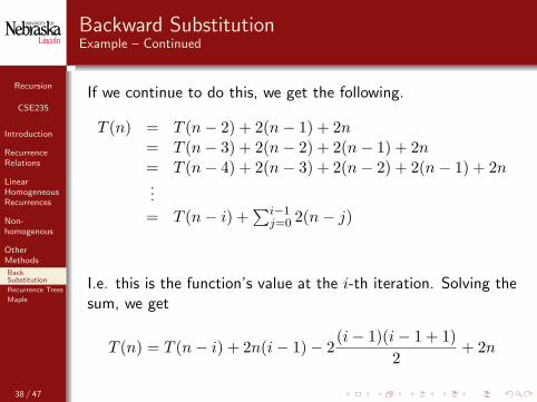
If we continue to do this, we get the following.
T (n) = T (n− 2) + 2(n− 1) + 2n= T (n− 3) + 2(n− 2) + 2(n− 1) + 2n= T (n− 4) + 2(n− 3) + 2(n− 2) + 2(n− 1) + 2n...
= T (n− i) +∑i−1
j=0 2(n− j)
I.e. this is the function’s value at the i-th iteration. Solving thesum, we get
T (n) = T (n− i) + 2n(i− 1)− 2(i− 1)(i− 1 + 1)
2+ 2n
38 / 47
Recursion
CSE235
Introduction
RecurrenceRelations
LinearHomogeneousRecurrences
Non-homogenous
OtherMethods
BackSubstitution
Recurrence Trees
Maple
Backward SubstitutionExample – Continued
If we continue to do this, we get the following.
T (n) = T (n− 2) + 2(n− 1) + 2n
= T (n− 3) + 2(n− 2) + 2(n− 1) + 2n= T (n− 4) + 2(n− 3) + 2(n− 2) + 2(n− 1) + 2n...
= T (n− i) +∑i−1
j=0 2(n− j)
I.e. this is the function’s value at the i-th iteration. Solving thesum, we get
T (n) = T (n− i) + 2n(i− 1)− 2(i− 1)(i− 1 + 1)
2+ 2n
38 / 47

Recursion
CSE235
Introduction
RecurrenceRelations
LinearHomogeneousRecurrences
Non-homogenous
OtherMethods
BackSubstitution
Recurrence Trees
Maple
Backward SubstitutionExample – Continued
If we continue to do this, we get the following.
T (n) = T (n− 2) + 2(n− 1) + 2n= T (n− 3) + 2(n− 2) + 2(n− 1) + 2n
= T (n− 4) + 2(n− 3) + 2(n− 2) + 2(n− 1) + 2n...
= T (n− i) +∑i−1
j=0 2(n− j)
I.e. this is the function’s value at the i-th iteration. Solving thesum, we get
T (n) = T (n− i) + 2n(i− 1)− 2(i− 1)(i− 1 + 1)
2+ 2n
38 / 47
Recursion
CSE235
Introduction
RecurrenceRelations
LinearHomogeneousRecurrences
Non-homogenous
OtherMethods
BackSubstitution
Recurrence Trees
Maple
Backward SubstitutionExample – Continued
If we continue to do this, we get the following.
T (n) = T (n− 2) + 2(n− 1) + 2n= T (n− 3) + 2(n− 2) + 2(n− 1) + 2n= T (n− 4) + 2(n− 3) + 2(n− 2) + 2(n− 1) + 2n
...
= T (n− i) +∑i−1
j=0 2(n− j)
I.e. this is the function’s value at the i-th iteration. Solving thesum, we get
T (n) = T (n− i) + 2n(i− 1)− 2(i− 1)(i− 1 + 1)
2+ 2n
38 / 47

Recursion
CSE235
Introduction
RecurrenceRelations
LinearHomogeneousRecurrences
Non-homogenous
OtherMethods
BackSubstitution
Recurrence Trees
Maple
Backward SubstitutionExample – Continued
If we continue to do this, we get the following.
T (n) = T (n− 2) + 2(n− 1) + 2n= T (n− 3) + 2(n− 2) + 2(n− 1) + 2n= T (n− 4) + 2(n− 3) + 2(n− 2) + 2(n− 1) + 2n...
= T (n− i) +∑i−1
j=0 2(n− j)
I.e. this is the function’s value at the i-th iteration. Solving thesum, we get
T (n) = T (n− i) + 2n(i− 1)− 2(i− 1)(i− 1 + 1)
2+ 2n
38 / 47
Recursion
CSE235
Introduction
RecurrenceRelations
LinearHomogeneousRecurrences
Non-homogenous
OtherMethods
BackSubstitution
Recurrence Trees
Maple
Backward SubstitutionExample – Continued
If we continue to do this, we get the following.
T (n) = T (n− 2) + 2(n− 1) + 2n= T (n− 3) + 2(n− 2) + 2(n− 1) + 2n= T (n− 4) + 2(n− 3) + 2(n− 2) + 2(n− 1) + 2n...
= T (n− i) +∑i−1
j=0 2(n− j)
I.e. this is the function’s value at the i-th iteration. Solving thesum, we get
T (n) = T (n− i) + 2n(i− 1)− 2(i− 1)(i− 1 + 1)
2+ 2n
38 / 47
Recursion
CSE235
Introduction
RecurrenceRelations
LinearHomogeneousRecurrences
Non-homogenous
OtherMethods
BackSubstitution
Recurrence Trees
Maple
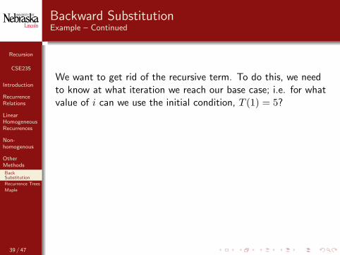
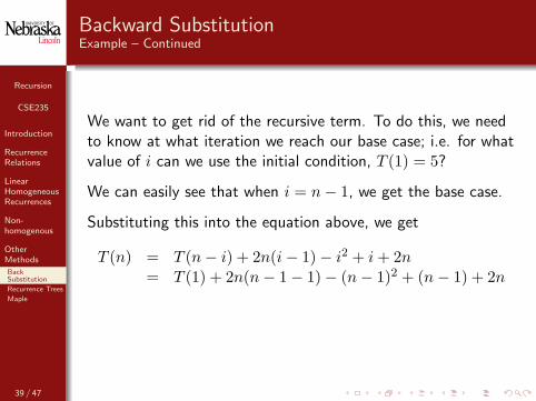
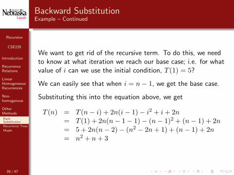
Backward SubstitutionExample – Continued
We want to get rid of the recursive term. To do this, we needto know at what iteration we reach our base case; i.e. for whatvalue of i can we use the initial condition, T (1) = 5?
We can easily see that when i = n− 1, we get the base case.
Substituting this into the equation above, we get
T (n) = T (n− i) + 2n(i− 1)− i2 + i + 2n= T (1) + 2n(n− 1− 1)− (n− 1)2 + (n− 1) + 2n= 5 + 2n(n− 2)− (n2 − 2n + 1) + (n− 1) + 2n= n2 + n + 3
39 / 47

Recursion
CSE235
Introduction
RecurrenceRelations
LinearHomogeneousRecurrences
Non-homogenous
OtherMethods
BackSubstitution
Recurrence Trees
Maple
Backward SubstitutionExample – Continued
We want to get rid of the recursive term. To do this, we needto know at what iteration we reach our base case; i.e. for whatvalue of i can we use the initial condition, T (1) = 5?
We can easily see that when i = n− 1, we get the base case.
Substituting this into the equation above, we get
T (n) = T (n− i) + 2n(i− 1)− i2 + i + 2n
= T (1) + 2n(n− 1− 1)− (n− 1)2 + (n− 1) + 2n= 5 + 2n(n− 2)− (n2 − 2n + 1) + (n− 1) + 2n= n2 + n + 3
39 / 47
Recursion
CSE235
Introduction
RecurrenceRelations
LinearHomogeneousRecurrences
Non-homogenous
OtherMethods
BackSubstitution
Recurrence Trees
Maple
Backward SubstitutionExample – Continued
We want to get rid of the recursive term. To do this, we needto know at what iteration we reach our base case; i.e. for whatvalue of i can we use the initial condition, T (1) = 5?
We can easily see that when i = n− 1, we get the base case.
Substituting this into the equation above, we get
T (n) = T (n− i) + 2n(i− 1)− i2 + i + 2n= T (1) + 2n(n− 1− 1)− (n− 1)2 + (n− 1) + 2n
= 5 + 2n(n− 2)− (n2 − 2n + 1) + (n− 1) + 2n= n2 + n + 3
39 / 47

Recursion
CSE235
Introduction
RecurrenceRelations
LinearHomogeneousRecurrences
Non-homogenous
OtherMethods
BackSubstitution
Recurrence Trees
Maple
Backward SubstitutionExample – Continued
We want to get rid of the recursive term. To do this, we needto know at what iteration we reach our base case; i.e. for whatvalue of i can we use the initial condition, T (1) = 5?
We can easily see that when i = n− 1, we get the base case.
Substituting this into the equation above, we get
T (n) = T (n− i) + 2n(i− 1)− i2 + i + 2n= T (1) + 2n(n− 1− 1)− (n− 1)2 + (n− 1) + 2n= 5 + 2n(n− 2)− (n2 − 2n + 1) + (n− 1) + 2n
= n2 + n + 3
39 / 47
Recursion
CSE235
Introduction
RecurrenceRelations
LinearHomogeneousRecurrences
Non-homogenous
OtherMethods
BackSubstitution
Recurrence Trees
Maple
Backward SubstitutionExample – Continued
We want to get rid of the recursive term. To do this, we needto know at what iteration we reach our base case; i.e. for whatvalue of i can we use the initial condition, T (1) = 5?
We can easily see that when i = n− 1, we get the base case.
Substituting this into the equation above, we get
T (n) = T (n− i) + 2n(i− 1)− i2 + i + 2n= T (1) + 2n(n− 1− 1)− (n− 1)2 + (n− 1) + 2n= 5 + 2n(n− 2)− (n2 − 2n + 1) + (n− 1) + 2n= n2 + n + 3
39 / 47
Recursion
CSE235
Introduction
RecurrenceRelations
LinearHomogeneousRecurrences
Non-homogenous
OtherMethods
BackSubstitution
Recurrence Trees
Maple
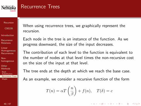
Recurrence Trees
When using recurrence trees, we graphically represent therecursion.
Each node in the tree is an instance of the function. As weprogress downward, the size of the input decreases.
The contribution of each level to the function is equivalent tothe number of nodes at that level times the non-recursive coston the size of the input at that level.
The tree ends at the depth at which we reach the base case.
As an example, we consider a recursive function of the form
T (n) = αT
(n
β
)+ f(n), T (δ) = c
40 / 47
Recursion
CSE235
Introduction
RecurrenceRelations
LinearHomogeneousRecurrences
Non-homogenous
OtherMethods
BackSubstitution
Recurrence Trees
Maple
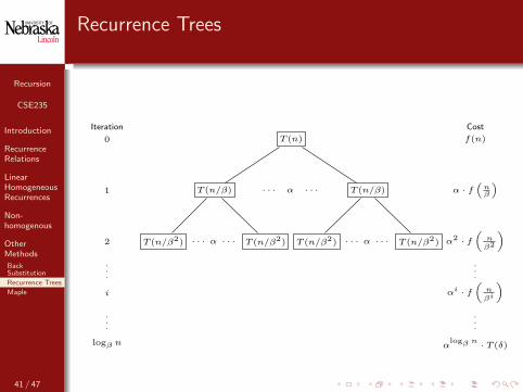
Recurrence Trees
T (n)
T (n/β)
T (n/β2) · · · α · · · T (n/β2)
· · · α · · · T (n/β)
T (n/β2) · · · α · · · T (n/β2)
Iteration
0
1
2
.
.
.
i
.
.
.
logβ n
Cost
f(n)
α · f“
nβ
”
α2 · f
„n
β2
«...
αi · f
„nβi
«...
αlogβ n · T (δ)
41 / 47
Recursion
CSE235
Introduction
RecurrenceRelations
LinearHomogeneousRecurrences
Non-homogenous
OtherMethods
BackSubstitution
Recurrence Trees
Maple
Recurrence TreesExample
The total value of the function is the summation over all levelsof the tree:
T (n) =logβ n∑i=0
αi · f(
n
βi
)
We consider the following concrete example.
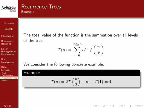
Example
T (n) = 2T(n
2
)+ n, T (1) = 4
42 / 47
Recursion
CSE235
Introduction
RecurrenceRelations
LinearHomogeneousRecurrences
Non-homogenous
OtherMethods
BackSubstitution
Recurrence Trees
Maple
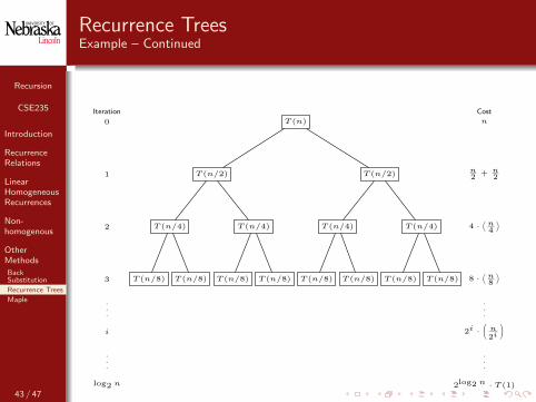
Recurrence TreesExample – Continued
T (n)
T (n/2)
T (n/4)
T (n/8) T (n/8)
T (n/4)
T (n/8) T (n/8)
T (n/2)
T (n/4)
T (n/8) T (n/8)
T (n/4)
T (n/8) T (n/8)
Iteration
0
1
2
3
.
.
.
i
.
.
.
log2 n
Cost
n
n2 + n
2
4 ·„
n4
«
8 ·„
n8
«
.
.
.
2i ·0@ n2i
1A
.
.
.
2log2 n · T (1)43 / 47
Recursion
CSE235
Introduction
RecurrenceRelations
LinearHomogeneousRecurrences
Non-homogenous
OtherMethods
BackSubstitution
Recurrence Trees
Maple
Recurrence TreesExample – Continued
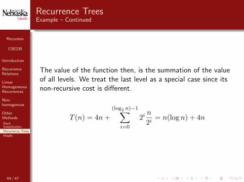
The value of the function then, is the summation of the valueof all levels. We treat the last level as a special case since itsnon-recursive cost is different.
T (n) = 4n +(log2 n)−1∑
i=0
2i n
2i= n(log n) + 4n
44 / 47
Recursion
CSE235
Introduction
RecurrenceRelations
LinearHomogeneousRecurrences
Non-homogenous
OtherMethods
BackSubstitution
Recurrence Trees
Maple
Smoothness Rule I
In the previous example we make the following assumption:that n was a power of two; n = 2k. This was necessary to geta nice depth of log n and a full tree.
We can restrict consideration to certain powers because of thesmoothness rule, which is not studied in this course. For moreinformation about the smoothness rule, please consult pages481–483 in the textbook “The Design & Analysis ofAlgorthims” by Anany Levitin.
45 / 47

Recursion
CSE235
Introduction
RecurrenceRelations
LinearHomogeneousRecurrences
Non-homogenous
OtherMethods
BackSubstitution
Recurrence Trees
Maple
How To Cheat With Maple I
Maple and other math tools are great resources. However, theyare not substitutes for knowing how to solve recurrencesyourself.
As such, you should only use Maple to check your answers.Recurrence relations can be solved using the rsolve commandand giving Maple the proper parameters.
The arguments are essentially a comma-delimited list ofequations: general and boundary conditions, followed by the“name” and variable of the function.
46 / 47
Recursion
CSE235
Introduction
RecurrenceRelations
LinearHomogeneousRecurrences
Non-homogenous
OtherMethods
BackSubstitution
Recurrence Trees
Maple
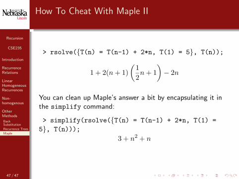
How To Cheat With Maple II
> rsolve({T(n) = T(n-1) + 2*n, T(1) = 5}, T(n));
1 + 2(n + 1)(
12n + 1
)− 2n
You can clean up Maple’s answer a bit by encapsulating it inthe simplify command:
> simplify(rsolve({T(n) = T(n-1) + 2*n, T(1) =5}, T(n)));
3 + n2 + n
47 / 47