Recursive Allocations and WealthDistribution with Multiple Goods:

Existence, Survivorship, and Dynamics

R. Colacito M. M. Croce Zhao Liu∗

————————————————————————————————————–

Abstract

We characterize the equilibrium of a complete markets economy with multipleagents featuring a preference for the timing of the resolution of uncertainty. Util-ities are defined over an aggregate of two goods. We provide conditions underwhich the solution of the planner’s problem exists, and it features a nondegen-erate invariant distribution of Pareto weights. We also show that perturbationmethods replicate the salient features of our recursive risk-sharing scheme, pro-vided that higher-order terms are included.

JEL classification: C62; F37.This draft: March 28, 2018.

————————————————————————————————————–∗Colacito is affiliated with the University of North Carolina at Chapel Hill, Kenan Flagler School

of Business. Croce is affiliated with the University of North Carolina at Chapel Hill, Kenan FlaglerSchool of Business, Bocconi University, and CEPR. Liu is a PhD student at Duke University, EconomicsDepartment. We thank our Editor Karl Schmedders and three anonymous referees. We also thankseminar participants at the 2009 Meeting of the Society for Economic Dynamics in Istanbul and at the2010 Meeting of American Economic Association in Atlanta. We are grateful to Lars Hansen, ThomasPhilippon, Tom Sargent and the participants at the 2010 PhD mini-course on Asset Pricing and RiskSharing with Recursive Preferences at NYU, which was partly based on this paper. All errors remainour own.

1 Introduction

In the context of single-agent economies, recursive preferences have become increas-

ingly relevant for the analysis of issues at the forefront of the macro-finance agenda

(see, among others, Hansen and Sargent (1995), Tallarini (2000), Bansal and Yaron

(2004), and Backus, Routledge and Zin (2005)). In models populated by multiple

agents, in contrast, the adoption of recursive preferences is less common, as it pro-

duces a key challenge in the characterization of the risk-sharing dynamics.

With recursive preferences, in fact, optimal allocations are a function not only of ag-

gregate endowment, but also of a possibly time-varying distribution of wealth. As

documented by Anderson (2005), in a one-good economy in which agents have risk-

sensitive preferences there is typically a tension between ensuring that a nonde-

generate distribution of wealth exists and having interesting heterogeneity across

agents.The same paper documents that this tension can be relaxed if multiple pref-

erence parameters are changed simultaneously and agents have power-reward func-

tions with risk aversion between zero and one.

In this paper, we overcome these challenges by focusing on an economy with multiple

goods. We show that rich dynamics of Pareto optimal allocations are obtained even

in the case in which all agents share the same risk-sensitivity parameter and have

logarithmic period reward functions, provided that they feature a different degree of

preference for one of the two goods. Furthermore, we provide conditions under which

a nondegenerate ergodic distribution of Pareto weights exists. This is the case in

which every agent in the economy has a strictly positive wealth in the long run.

An agent with recursive preferences is willing to trade off expected utility for higher

1

conditional moments of future utility. In a world with a Cobb-Douglas aggregate over

multiple goods, the intensity of this trade-off is stronger for agents that consume a

large share of aggregate resources, that is, agents with high Pareto weights. For

example, as shown in a simple two-period model, when agent 1 has a high initial

share of resources, she will have a strong incentive to buy insurance from agent 2 to

mitigate future utility uncertainty.

In equilibrium, under a preference for early resolution of uncertainty, agent 1 accepts

a reduction in her expected average share of resources (i.e., her Pareto weight is ex-

pected to decline) in exchange for a reduction of future utility variance. This trade-off

between expected utility and conditional volatility of future utility results in a well-

defined invariant distribution of Pareto weights.

Several authors have documented the theoretical properties of one-good versions of

the economy analyzed in this paper (Lucas and Stokey (1984), Ma (1993), and Kan

(1995)). In particular, Anderson (2005) shows that in an economy with heterogenous

agents and recursive preferences it is difficult to ensure the existence of a nondegen-

erate ergodic distribution of wealth, unless very extreme forms of heterogeneity are

considered (see, for example, Backus, Routledge and Zin (2009)).

Our focus on the case of a consumption aggregate of multiple goods resolves these

problems, and it is important in many economic applications. In a closed economy, we

may think of agents featuring different propensities across commodities produced by

different firms or sectors. In an open economy, it is common to assume that consumers

located in different countries are biased toward the consumption of the domestically

produced good (see, for example, Tretvoll (2016)). The economy analyzed in this paper

provides the foundations for the international macro-finance model in Colacito and

2

Croce (2013). In related work Backus, Coleman, Ferriere and Lyon (2016) show that

the endogenous variation in Pareto weights in the type of economies that we consider

can be interpreted as wedges from the perspective of a frictionless model with additive

preferences.

Colacito and Croce (2012) apply the results in this manuscript to the heterogeneous-

beliefs literature (among others, see Kubler and Schmedders (2012) and Tsyrennikov

(2012)).1 They show that consumption home bias is isomorphic to endogenous dis-

agreement about the fundamentals of the economy. Under the conditions explored in

our paper, the ergodic distribution of wealth is nondegenerate, despite the existence

of endogenous heterogenous beliefs. For a detailed study of both the survivorship and

risk sharing in economies populated by recursive agents with exogenous heteroge-

neous beliefs see Borovicka (2016).

From a computational point of view, the characterization of the risk-sharing arrange-

ment with recursive preferences poses additional challenges, as the state space in-

cludes the relative wealth of the agents, which in turn, depends on the continua-

tion utilities. We compare a global method that uses value-function iterations and a

perturbation-based approach and document that a first-order Taylor expansion about

the stochastic steady state of the economy is not appropriate for capturing the dy-

namics of the economy. This approximation severely deteriorates in regions distant

from the steady state, and it produces a counterfactual limiting wealth distribution

in which either agent may find herself with zero wealth with probability one. Higher-

order approximations are necessary not only to provide a better period-by-period char-1Specifically, Colacito and Croce (2012) interpret the preferences used in this manuscript as describ-

ing a concern for model misspecification, according to the definition of Hansen and Sargent (2008).This results in agent-specific distorted conditional distributions of the endowment processes. Sinceeach probability depends on the utility of a specific agent, when preferences feature heterogenous biasacross goods, agents disagree on the transition probabilities across states of the world.

3

acterization of the dynamics of the model, but also to capture the stationarity of the

model. These findings are consistent with the analysis of Anderson, Hansen and Sar-

gent (2012) and Pohl, Schmedders and Wilms (2016).

Additionally, we show that our setting produces endogenous time variation in higher-

order conditional moments of consumption, and hence it offers general equilibrium

foundations for the analyses of Bansal, Kiku, Shaliastovich and Yaron (2014), Kuehn

and Boguth (2013), Colacito, Ghysels, Meng and Siwarasit (2016), and Segal, Shalias-

tovich and Yaron (2015).

We also study important extensions of our benchmark model by considering the case

in which agents have intertemporal elasticities of substitution different from 1 and

endowment shocks that are persistent. This means that our analysis can be infor-

mative for the growing body of the literature that has explored the macro-finance

implications of Epstein and Zin (1989) preferences (see, for example, Bansal et al.

(2014)). Furthermore, we show that the introduction of a moderate degree of het-

erogeneity in the calibration of the two countries may still result in a well-defined

ergodic distribution of wealth in equilibrium. This is relevant for the application of

our study to economies in which, for example, investors in different countries face a

heterogeneous degree of fundamental risk in their endowments or productivities.

Baker and Routledge (2017) study an economy similar to the one analyzed in this

paper. Like us, they consider the risk-sharing arrangement between two agents with

recursive preferences defined over a Cobb-Douglas aggregate of two goods: oil and a

general consumption good. Since the main focus of their paper is matching the price

of oil and related futures contracts, they rely on asymmetric calibrations of the two

agents. This choice typically results in the survivorship of only one of the two agents

4

in the economy. In this respect, the results that we provide in section 5, in which we

relax the symmetry of the calibration, are informative for the general class of model

that they consider.

Our paper is organized as follows. In section 2 we provide the setup of our benchmark

economy, featuring unit intertemporal elasticity of substitution and i.i.d. shocks. In

section 3 we discuss the main intuitions of our framework in the context of a simple

two periods model and provide the set of conditions under which a nondegenerate lim-

iting distribution of Pareto weights exists in the infinite horizon setting. In section 4

we compare a numerical solution of the model obtained via value function iteration

with first and higher order approximations. In section 5 we present the results of

several generalized versions of our baseline setup. Section 6 concludes the paper.

2 Setup of the Economy

In this section, we describe the assumptions that we use in the benchmark version of

our model. For the purpose of simplifying the analytical proofs and the intuitions of

the model, in our benchmark we assume that the intertemporal elasticity of substi-

tution is equal to one and that the two countries share a symmetrical calibration. In

section 5, we use simulations to show that our results apply to more general settings.

The following three assumptions about preferences, consumption, and endowments

will be retained throughout the rest of the paper.

Assumption 1 (Preferences). Let there be two agents, indexed by 1 and 2, whose

5

preferences are recursively defined as

Ui(ci, qi) = (1− δi) log ci + δiθi log∑z′

π(z′) exp

qi(z

′)

θi

, ∀i ∈ 1, 2, (1)

where qi(z′) gives the utility remaining from the next period on when next-periods state

is z′. For each agent i, θi < 0.

This class of preferences can be interpreted in several ways. First, they correspond

to the case of risk-sensitive preferences studied by, among others, Hansen and Sar-

gent (1995), Tallarini (2000), and Anderson (2005). Second, they coincide with a

log-transformation of Epstein and Zin (1989) preferences in the case in which the

intertemporal elasticity of substitution is equal to one. In this case, the risk-sensitive

parameter, θ, is related to risk aversion, γ, by imposing

θ =1

1− γ.

In this paper, we focus on a discrete time setting as opposed to the continuous time

approach of Epstein (1987), Duffie, Geoffard and Skiadas (1994), Geoffard (1996), and

Dumas, Uppal and Wang (2000).

Since these preferences depart from the expected utility case, higher moments of con-

tinuation utilities matter for the determination of optimal risk sharing. As as exam-

ple, if continuation utilities qi(z′) are normally distributed, the functional form in (1)

can be written as

Ui(ci, qi) = (1− δi) log ci + δiEi(qi) +δi2θi

Vi(qi), ∀i ∈ 1, 2, (2)

6

where

Ei(qi) =∑z′

π(z′)qi(z′)

Vi(qi) =∑z′

π(z′)

[qi(z

′)−

(∑z′

π(z′)qi(z′)

)]2

are the conditional mean and variance of the continuation utility, respectively.

Although we will work with the general specification in (1), equation (2) is instructive,

since it intuitively shows that when the parameters θi’s are less than zero, the risk-

sharing scheme must account for an efficient endogenous trade-off between utility

level and utility variance.

As the dynamics of second-order moments are crucial for characterizing the equilib-

rium of the model, in section 4 we also assess the accuracy of several approximations

based on how well they can account for the dynamics of volatilities.

Assumption 2 (Consumption bundles). Let consumption ci be an aggregate of two

goods, xi and yi. Specifically, let

ci = (xi)λi (yi)

1−λi (3)

be the consumption bundle, with λ1 > 1/2 and λ2 < 1/2 so that the two agents have a

bias for different goods.

This assumption generalizes the one-good framework studied by Anderson (2005),

which obtains as the special case in which λi = 1/2, ∀i, that is, the case in which there

is no preference bias across goods and hence we are effectively in a one-good economy.

7

The next assumption pertains to the endowment process and is common to Anderson

(2005):

Assumption 3 (Endowments). The endowment of the two goods follows a first-order

time-homogenous Markov process (z0, z1, ...) which takes values in a finite set N =

1, ..., n. The aggregate supply of the two goods at time t is such that 0 < Xt = X(zt) <

∞, and 0 < Yt = Y (zt) <∞.

Finally, we need to make sure that the preference parameters are chosen so that the

utility recursion converges:

Assumption 4 (Contraction). The parameters λi, γi, δi are such that the right-hand

side of equation (1) has a modulus smaller than one, ∀i = 1, 2.

Recursive planner’s problem. Let logW ∗i (z, ci, qi,z′z′) be the right-hand side of

equation (1). Given the conditions specified by Ma (1993) and Ma (1996), the social

planner’s value function, denoted as Qp(z, µ1) : N × [0, 1] → R, satisfies the following

functional equation proposed by Lucas and Stokey (1984) and Kan (1995):

Qp(z, µ1) = maxxi,yi,qi,z′i∈1,2,z′∈N

2∑i=1

µi logW ∗i (z, ci, qi,z′z′) (4)

subject toµ2 = 1− µ1

0 ≤ x1 ≤ X(z), 0 ≤ x2 ≤ X(z)− x1

0 ≤ y1 ≤ Y (z), 0 ≤ y2 ≤ Y (z)− y1

ci = (xi)λi (yi)

1−λi , ∀i = 1, 2

0 ≤ minµ1(z′)∈[0,1]

Qp(z′, µ1(z′))− µ1(z′)q1,z′ − (1− µ1(z′))q2,z′ ∀z′ ∈ N . (5)

Differentiability and first-order conditions. Let the ratio of the Pareto weights

8

be defined as

S =µ1

µ2

=µ1

1− µ1

.

Let Ui(z, S), i = 1, 2, denote the utility function of agent i evaluated at the optimum

when the exogenous state is z, and S ∈ (0,∞). On a consumption path that is bounded

away from zero, Ui(z, S) is differentiable (see Kan (1995) and Anderson (2005)) and

dUidµi

> 0 µ1 ∈ (0, 1), µ2 = 1− µ1.

On a consumption path that is bounded away from zero for both agents, Qp(s, µ1) is

also differentiable with respect to µ1 ∈ (0, 1). The optimality condition in equation (5)

implies that

dQp

dµ1

(z, µ1) = U1(z, S)− U2(z, S), µ1 ∈ (0, 1) (6)

d2Qp

dµ21

(z, µ1) =dU1

dµ1

(z, S) +dU2

dµ2

(z, S) > 0. (7)

Therefore,Qp(s, µ1) is strictly convex with respect to µ1, as in Lucas and Stokey (1984).

This is relevant because it implies that the unique optimal policy of the planner can

be characterized using first-order conditions.

According to the first-order conditions, for a given S, the optimal allocation of goods

satisfies the following system of equations common to all static Pareto problems with

two goods and two agents:

(1− δ1)∂ log c1

∂x1

· S = (1− δ2)∂ log c2

∂x2

(8)

(1− δ1)∂ log c1

∂y1

· S = (1− δ2)∂ log c2

∂y2

X = x1 + x2, Y = y1 + y2.

9

The optimal dynamic adjustment of the ratio of the pseudo-Pareto weights is then

given by

S ′ = S · M (z′, S ′) (9)

where

M (z′, S ′) ≡ δ1 exp U1 (z′, S ′) /θ1∑z′ π(z′) exp U1 (z′, S ′) /θ1

·∑

z′ π(z′) exp U2 (z′, S ′) /θ2δ2 exp U2 (z′, S ′) /θ2

.

Equation (9) determines the dynamics of the ratio of the Pareto weights and implicitly

generates a continuous function that we denote by fS(z′, ·) : [0,+∞)→ [0,+∞):

S ′ = fS (z′, S) . (10)

Characterizing the planner’s problem through first-order conditions is useful because

it allows us to represent the planner’s problem in (4) as a simple system of first-order

stochastic difference equations, namely (1), (3), (8), and (9). In the next section, we

use perturbation methods to solve our dynamic system of equations.

Relative price of the two goods. The relative price of the two goods, p, is the

equilibrium marginal rate of substitution across goods

p =(1− λ1)

λ1

· x1

y1

.

Given the optimal allocations of x1 and y1, we can write the relative price as

p = p · XY,

10

where

p ≡ (1− λ1)/λ1 ·[1 + S · (1− λ1)

(1− λ2)

]/[1 + S · λ1

λ2

].

When the supply of good X relative to good Y is high, the price of good Y increases

for two reasons. First, the last term (X/Y ) directly affects the relative price. This

channel would be at work even for λ1 = 1/2, in which case p = 1, and p = X/Y .

Second, since λ1 > λ2 it follows that

∂p

∂S= −1− λ1

λ1

· λ2

1− λ2

· (λ1 − λ2)

(λ2 + λ1 · S)2 < 0.

This means that the price will further increase as long as the ratio of Pareto weights

(S) declines when X/Y is large (we prove this statement formally in proposition 1).

Equivalently, the price of good Y is large whenever its supply is low. This effect

is magnified in the context of our model since λ1 > 1/2, λ2 < 1/2, and the ratio of

Pareto weights can move away from a symmetric wealth distribution. This enhanced

price adjustment allows agent 2 to purchase a larger share of resources whenever the

supply of its most preferred good is low.

Share of world consumption (SWC). We note that under our Cobb-Douglas ag-

gregator across goods, the relative share of world consumption of agent 1, SWC,

evolves as follows:

SWC =x1 + py1

X + pY=

S

1 + S= µ1. (11)

According to equations (8) and (11), the Pareto weight of agent 1 has a simple eco-

nomic interpretation, namely, the relative size of consumption allocated to agent 1.

11

Symmetry. So far, we have not imposed any specific assumptions on the conditional

probability of the Markov chain governing the supply of the two goods, nor have we

imposed any special restrictions on the preference parameters of our agents. In order

to have a well-specified problem, all we need is that assumptions 1–4 hold. In what

follows, however, we list further restrictions that are necessary to analytically char-

acterize the main properties of the optimal risk-sharing policy of the planner. These

conditions impose symmetry and are sufficient, but in many cases not necessary, for

the existence of a stationary distribution. In the next section, we relax many of these

assumptions.

Assumption 5 (Symmetrical preferences). Let the preference parameters δi and θi be

identical ∀i ∈ 1, 2. Let the consumption-bundle’s parameters be symmetrical across

agents, that is, λ1 = 1− λ2 > 1/2.

Assumption 6 (Balanced endowment space). Let the support of the endowment of

good X be given by the vector H = [h1, h2, ..., hN ]. Let the support of the endowment

of good Y be H as well. The endowments of the two goods take values in the finite

set N , given by all possible pairwise permutations of H. We refer to N as a balanced

endowment space.

Definition 1 (Symmetric states). Let the states zi, z−i ∈ N be such that zi = Xi =

X(i), Yi = Y (i) and z−i = X−i = Y (i), Y−i = X(i). Then zi and z−i are symmetric

states.

Finally, just to simplify our proof, we focus on a setting with i.i.d. shocks and on

symmetric probability distributions.

Assumption 7 (i.i.d. case). Assume that π(z′|z) = π(z′) > 0 ∀z, z′ ∈ N .

12

Assumption 8 (Symmetric probabilities). Let the states zi, z−i ∈ N be symmetric.

Then π(zi) = π(z−i).

3 Characterizing the Distribution of Pareto Weights

In this section, we show the main properties of the Pareto weights under our recursive

scheme in two settings. We start with a simplified two-period model for which we have

a closed-form approximate solution. We then provide results for our infinite-horizon

economy.

3.1 Recursive risk-sharing in a two-period model

The goal of this section is to illustrate the role of the income and substitution effects as

a function of the initial Pareto weights. To highlight the key features of the model, we

focus on the special case in which symmetry applies, consistent with the assumptions

employed for our main propositions. In Appendix A, we study a two-period version

of the planner’s problem detailed in the system of equations (4)–(5) and provide a

general solution which allows for asymmetries across the two agents.

Specifically, consider the following Pareto problem:

maxX1

1 ,X21 ,Y

11 ,Y

21 µ0 · θ logE0

[exp

u1

1

θ

]+ (1− µ0) · θ logE0

[exp

u2

1

θ

],

subject to the following conditions:

ui1 = log(Ci

1

), ∀i = 1, 2,

13

C11 =

(X1

1

)λ (Y 1

1

)(1−λ), C2

1 =(X2

1

)(1−λ) (Y 2

1

)λ.

and the following resource constraints:

X11 +X2

1 = eξ, Y 11 + Y 2

1 = e−ξ, ξ ∼ N(0, σ2),

where, for simplicity, we are assuming that the endowments of the two goods are

perfectly negatively correlated. Let s = log(µ0/(1 − µ0)) and let s be the log-ratio of

the pseudo-Pareto weights at time 1. We use this simple setup to illustrate three key

features of this class of models.

Income and substitution effects. We show in Appendix A that the equilibrium

utility functions can be written as

ui1 = ui1 + λξui1· ξ, ∀i = 1, 2, (12)

where

λξu1

1= (2λ− 1)︸ ︷︷ ︸

>0

1 +2β (s)

θ − β (s) (1 + es)︸ ︷︷ ︸<0

, and λξu2

1= − (2λ− 1)︸ ︷︷ ︸

>0

1 +2β (s) es

θ − β (s) (1 + es)︸ ︷︷ ︸<0

with β (s) defined as the following non-negative, and monotonically decreasing func-

tion of s:

β (s) =

[λ(1− λ)

(1− λ) + λes+

λ(1− λ)

λ+ (1− λ)es

].

Without loss of generality, let us focus on the response of agent 1’s utility to an endow-

ment shock ξ, which is captured by the coefficient λξu1

1. A positive endowment effect,

measured by (2λ− 1), determines an increase in the utility that is proportional to the

14

degree of preference for good X. In a single-agent economy, that is, for s → +∞, this

is the only effect relevant for the dynamics of future utilities. In a multiple-agent

economy, an additional negative redistribution effect captures the reallocation of re-

sources that takes place by virtue of risk sharing. This effect depends on β(s), and

hence it declines with the original ratio of Pareto weights, s.

Redistribution of resources. Using the equilibrium utilities in (12), it is easy to

show that the transition dynamics of the logarithm of the ratio of the Pareto weights

in (9) becomes

s− s =u1

1

θ− u2

1

θ−[E0 (u1

1)

θ+V ar0 (u1

1)

2θ2

]+

[E0 (u2

1)

θ+V ar0 (u2

1)

2θ2

](13)

=

[V ar0 (u2

1)

2θ2− V ar0 (u1

1)

2θ2

]+ λξs · ξ,

where

λξs =λξu1

1− λξ

u21

θ=

2(2λ− 1)

θ − β (s) (1 + es)

is the elasticity of the log-ratio of the Pareto weights with respect to the underlying

shock.

When λ > 1/2 and θ < 0, then λξs < 0. This means that when the supply of good X

is relatively scarce (i.e., ξ < 0), agent 1, whose preferences are relatively more tilted

toward the consumption of this good, is compensated by means of a greater transfer

of resources (i.e., s increases). If λ = 1/2, then the reallocation is null (λξs = 0).

This is a relevant case to consider because it corresponds to the situation in which

the multiple-goods economy is equivalent to a one-good economy. As documented by

Anderson (2005), in such an economy the distribution of resources is constant over

time, unless preference heterogeneity is introduced.

15

Conditional expectation of s − s. We can characterize the drift in the log-ratio of

the Pareto weights in equation (13) as follows:

[V ar0 (u2

1)

2θ2− V ar0 (u1

1)

2θ2

]=

σ2

2θ2

[(λξu2

1

)2

−(λξu1

1

)2]

=σ2β (s) (2λ− 1)

θ − β (s) (1 + es)︸ ︷︷ ︸<0

·(θ−1λξs

)︸ ︷︷ ︸>0

· (es − 1) .

The value of the drift is pinned down by precautionary motives related to continuation

utility variance. When the consumption share of agent 1 rises (i.e., s > 0), agent 1

wants to buy an increasing amount of insurance from agent 2. In equilibrium, agent

1 accepts a reduction in her expected average share of resources (i.e., the drift in

(s− s) is negative) in exchange for a reduction in future utility variance. At the same

time, agent 2 provides limited insurance at a higher price to agent 1 and expects

to receive a greater future consumption share.2 In Appendix A, we quantify this

intuition further and show that the expected growth of the agent with the smaller

consumption share increases with a larger degree of preference for one of the two

goods (λ), more fundamental risk (σ2), and stronger risk sensitivity (θ).

3.2 Infinite-horizon model

In this section, we prove that under symmetry a nondegenerate limiting distribution

of Pareto weights exists. Equivalently, in the limit no agent receives a Pareto weight

of zero with probability one. Furthermore, we characterize the adjustment of the

Pareto weights as a function of the realization of the shocks, and the conditional

expectation of the Pareto weights as a function of the current state of the economy.2We report the budget constraints associated to the decentralized economy in Appendix A.

16

An illustrative example. We introduce a simple example used in the subsequent

sections to better illustrate the properties of the model. Endowments can take on one

of the following four equally likely pairs of realizations:

N = (X = 103, Y = 103), (X = 103, Y = 100), (X = 100, Y = 103), (X = 100, Y = 100) .

We assume that the coefficient λ1 = 1 − λ2 = 0.97 so that agent 1 enjoys a higher

period utility when the supply of good X is large and agent 2 is better off when good

Y is more abundant. The risk-sensitive parameter θ is set to (1 − γ)−1 where γ = 25

in order to enhance the role of risk-sensitivity in this basic setup. We consider lower

values of risk aversion in sections 4 and 5. The qualitative implications of the model

are the same as long as γ > 1. For both agents, the subjective discount factor, δ, is set

to 0.96 to ensure fast convergence of our algorithm.

Ranking of Pareto weights. We use the following proposition to characterize the

ranking of Pareto weights as a function of the state of the economy.

Proposition 1. Let assumptions (1)–(8) hold. Let the events a, b ∈ N be such that

X ′(a)/Y ′(a) > X ′(b)/Y ′(b).

Then the ratio of Pareto weights is such that

S ′(a, S) ≤ S ′(b, S).

If X ′(a)/Y ′(a) = X ′(b)/Y ′(b), then S ′(a, S) = S ′(b, S).

Proof. See Appendix B.1.

17

0 0.2 0.4 0.6 0.8 1−5

0

5x 10

−6 X=103, Y=103

0 0.2 0.4 0.6 0.8 1−3

−2.5

−2

−1.5

−1

−0.5

0x 10

−3 X=103, Y=100

0 0.2 0.4 0.6 0.8 10

0.5

1

1.5

2

2.5

3x 10

−3 X=100, Y=103

0 0.2 0.4 0.6 0.8 1−5

0

5x 10

−6 X=100, Y=100

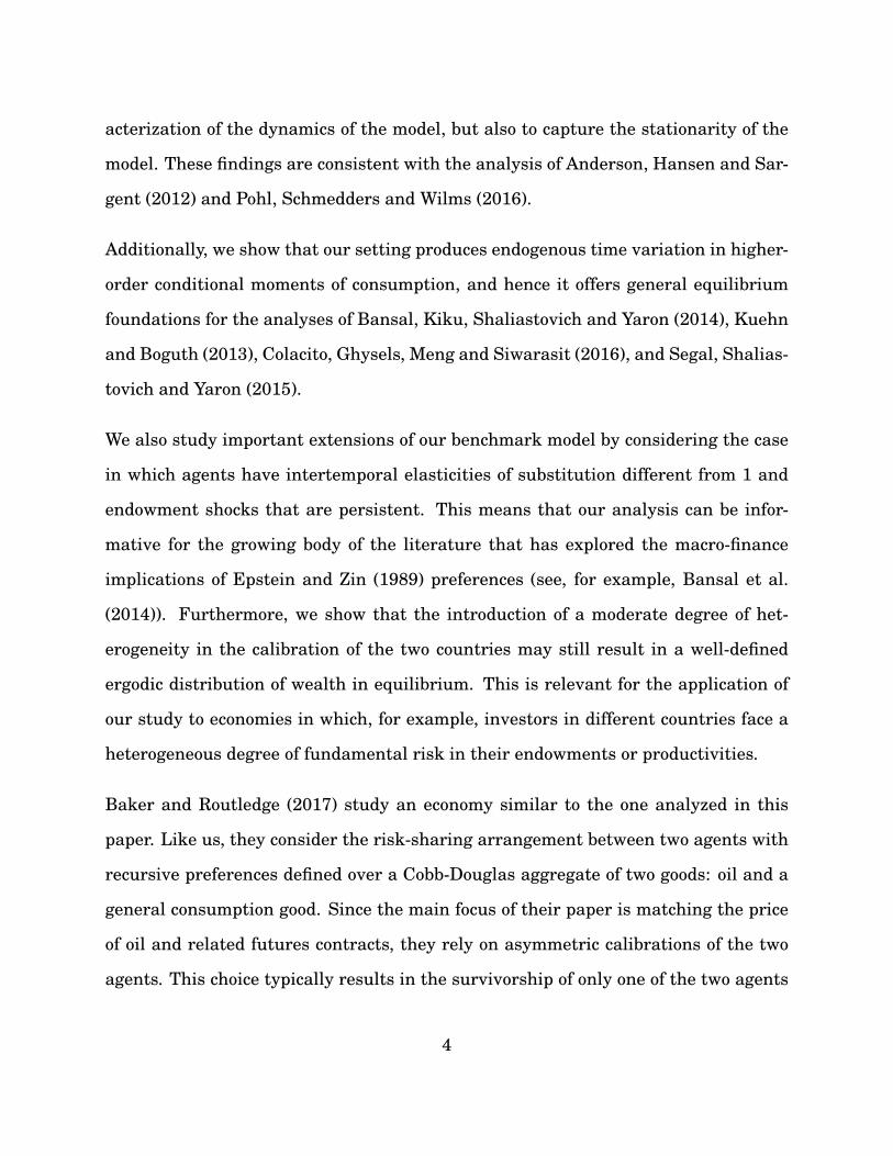
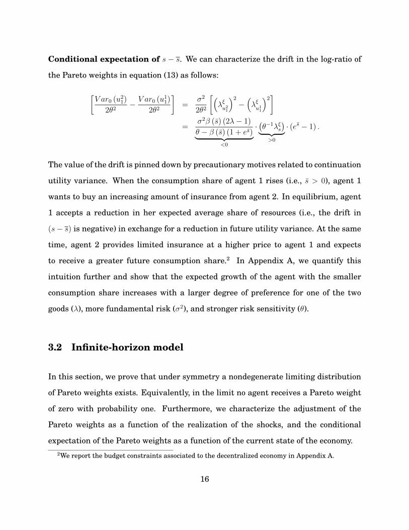
Figure 1: Phase diagrams of Pareto weights. Each panel refers to a different realization ofthe endowment of the two goods at time t + 1, zt+1 = [Xt+1 Yt+1]. On the vertical axis, wedepict the difference between the future Pareto weight for agent 1, µ1,t+1 = fµ1(zt+1, µ1,t), andits current value, µ1,t. On the horizontal axis we have µ1,t.

The interpretation of proposition 1 is simple: whenever agent 1 receives a good shock

to the endowment of the good that she likes the most, the social planner reduces her

weight. This reallocation enables agents 1 and 2 to share part of the endowment

risk of the economy, and it is consistent with what is shown in our two-period model,

where we document that the elasticity λξu1

1is negative. Furthermore, if the two goods

are in identical supply, the optimal choice of Pareto weights is independent of the

supply level.

Figure 1 documents this ranking by showing the optimal policies associated with our

illustrative example. First, notice that the optimal policy is identical in the two states

18

0 0.1 0.2 0.3 0.4 0.5 0.6 0.7 0.8 0.9 10

0.01

0.02

0.03

0.04

0.05

0.06

0.07

0.08

0.09

0 0.1 0.2 0.3 0.4 0.5 0.6 0.7 0.8 0.9 1-8

-6

-4

-2

0

2

4

6

8

E(

-)

10-6

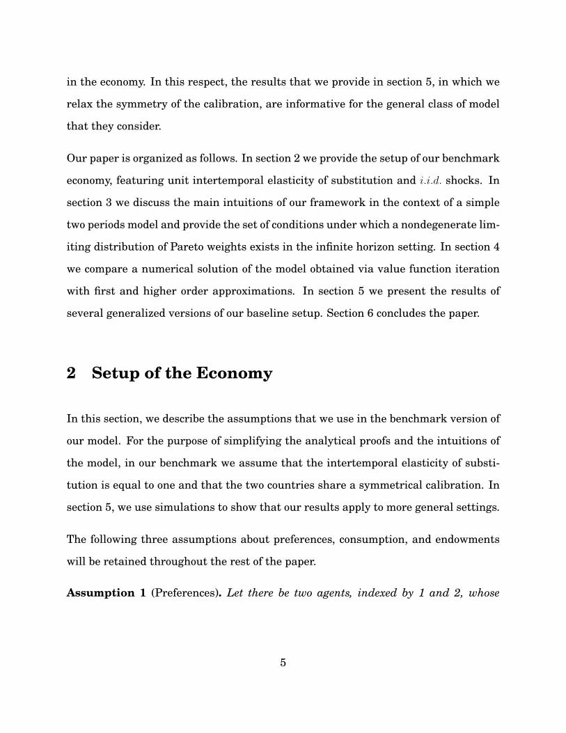
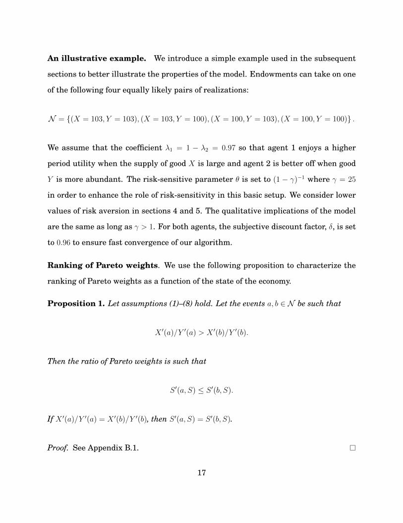
Figure 2: Survivorship. The left panel reports the invariant distribution of the Pareto weightof agent 1 (µ1). The right panel shows the conditional expectation of the Pareto weight incre-ment for agent 1, E[µ′1 − µ1|µ1], as a function of the current µ1.

of equal supply of the two goods (see the top-left and the bottom-right panel). Second,

notice that next-period’s Pareto weight attached to agent 1 is lower when the supply

of good X is relatively more abundant (top-right panel) than it is when the supply of

good X is relatively more scarce (lower-left panel).

The distribution of the Pareto weights: ergodicity and mean reversion. We

document that in the limit no agent receives a Pareto weight of zero with probability

one. Furthermore, it is possible to demonstrate that in our economy the dynamics

of Pareto weights are characterized by mean reversion. This means that when the

Pareto weight of any agent is small (large), it is expected to increase (decrease) going

forward. The following two propositions formalize these statements.

Proposition 2. Let assumptions (1)–(8) hold. The stochastic processes µ1 and µ2 can-

not converge to either 0 or 1 almost surely.

Proof. See Appendix B.2.

19

Proposition 3. Let assumptions (1)–(8) hold. The expectation of the next-period’s

Pareto weight on agent 1 conditional on the current Pareto weight is such that (i)E[µ′1|S]

=

µ1, if µ1 = 12; (ii) E

[µ′1|S]< µ1, ∀µ1 ∈

(12, 1)

; and (iii) E[µ′1|S]> µ1,∀µ1 ∈

(0, 1

2

).

Proof. See Appendix B.3.

The content of propositions 2 and 3 is depicted in figure 2. The left panel of figure 2

shows that the invariant distribution of Pareto weights does not display any mass

in the limiting cases of µ1 = 0, 1. This means that in the long run both agents

“survive,” that is, they both consume a nonzero share of the aggregate resources.

The right panel of figure 2 shows that the conditional change in the Pareto weight

of each agent is positive when the Pareto weight is small, and negative when the

Pareto weight is large. Equivalently, the dynamics of the Pareto weight feature mean

reversion, which is due to endogenous asymmetries in precautionary saving motives.

Taken together, propositions 2 and 3 ensure the existence of a well-defined invariant

distribution of Pareto weights.

As in our two-period economy, the substitution effect generated by the reallocation

channel is size dependent due to the nonlinearity of the aggregator of the two goods.

An agent with a large share of consumption benefits the least from the substitution

effect and is willing to buy very expensive insurance from the other agent in order

to reduce the conditional variance of her continuation utility. As a result, the agent

with a small consumption share is expected to receive a positive transfer of resources

going forward, and her consumption share is expected to become larger.

20

4 Comparison of Approximations

In this section we investigate the ability of both first- and higher-order approxima-

tions to capture the short- and long-run characteristics of the model. In order to

use common perturbation techniques, we assume that endowments are jointly log-

normally distributed, with the following means and covariance matrix:

logX

log Y

∼ N

4.62

4.62

, 0.0252 0.3 · 0.0252

0.3 · 0.0252 0.0252

.

This calibration captures the degree of correlation of output (Colacito and Croce

(2013)).

In what follows we show that the results with Gaussian shocks are similar to those

obtained with a finite discretized joint normal distribution. This constitutes a gener-

alized setup relative to our earlier sections, which will prove important in allowing us

to numerically analyze several interesting extensions of our benchmark model in sec-

tion 5. Specifically, we discretize the distribution of the exogenous endowment shocks

on a 21× 21 grid of equally spaced nodes on the range

[exp4.62− 5× 0.025, exp4.62 + 5× 0.025] .

We set δ = 0.96, λ1 = 0.97, and γ = 15. This value of risk aversion is in line with

those typically employed in the equity premium puzzle literature (see, among others,

Tallarini (2000)) and can be lower than that used in section 3.2 because we adopt a

richer set of exogenous states.

The curse of the linear approximation. A first-order Taylor approximation about

21

0 0.5 1 1.5 2 2.5 3 3.5 4

x 105

0

0.2

0.4

0.6

0.8

1

Time

µ 1

Actual

First Order Approximation

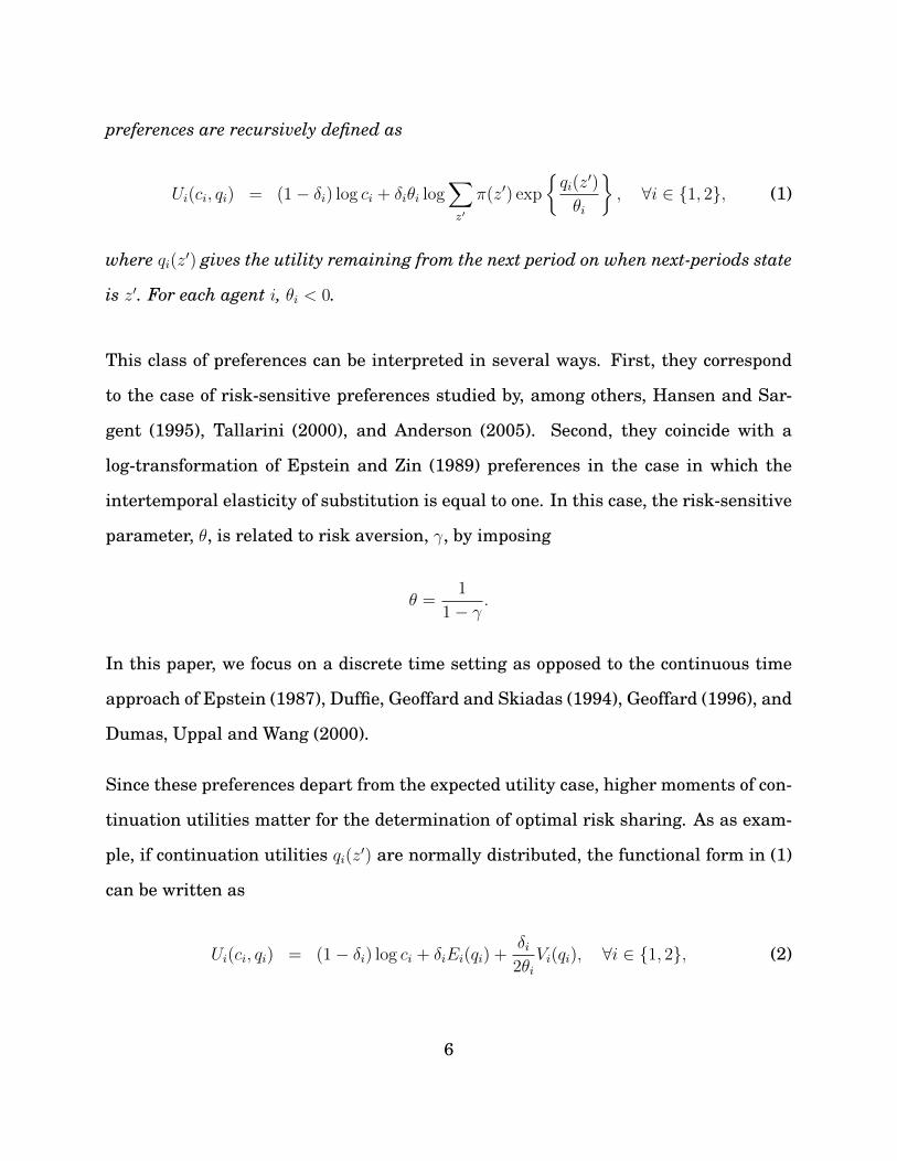
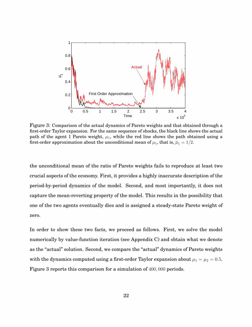
Figure 3: Comparison of the actual dynamics of Pareto weights and that obtained through afirst-order Taylor expansion. For the same sequence of shocks, the black line shows the actualpath of the agent 1 Pareto weight, µ1, while the red line shows the path obtained using afirst-order approximation about the unconditional mean of µ1, that is, µ1 = 1/2.

the unconditional mean of the ratio of Pareto weights fails to reproduce at least two

crucial aspects of the economy. First, it provides a highly inaccurate description of the

period-by-period dynamics of the model. Second, and most importantly, it does not

capture the mean-reverting property of the model. This results in the possibility that

one of the two agents eventually dies and is assigned a steady-state Pareto weight of

zero.

In order to show these two facts, we proceed as follows. First, we solve the model

numerically by value-function iteration (see Appendix C) and obtain what we denote

as the “actual” solution. Second, we compare the “actual” dynamics of Pareto weights

with the dynamics computed using a first-order Taylor expansion about µ1 = µ2 = 0.5.

Figure 3 reports this comparison for a simulation of 400, 000 periods.

22

For the first part of the simulation, the Pareto weights are in the relatively small

neighborhood of 0.5. In this region, the first-order Taylor expansion does a good job

of approximating the actual dynamics of the economy. The approximation, however,

starts deteriorating significantly as the economy departs from µ1 = 0.5. On this his-

tory, according to the first-order Taylor expansion, the Pareto weight of agent 1 should

level off at zero, even though this is in sharp contrast to the actual dynamics of the

model and the survivorship results explained in the previous sections. As a conse-

quence, the long-run implications of the first-order Taylor expansion are unreliable.

In this clear-cut example, what may at first look like a small error results in an ir-

reversible misrepresentation of the actual dynamics of the economy and its long-run

moments. In this economy, higher-order approximations are needed not only to pro-

vide a more accurate description of the period-by-period dynamics, but also to pre-

serve the existence of a well-defined ergodic distribution.

The case for higher-order approximations. The linear approximation does not

accurately describe the dynamics of the Pareto weights because it impels a first-order

integrated process. This is clearly depicted in the left panel of figure 4, in which we

compare the expected growth of the ratio of Pareto weights as a function of the current

ratio across different solution methods. The flat line for the first-order approximation

suggests that the conditional expected change of the ratio of Pareto weights is identi-

cally zero, implying the lack of any kind of mean reversion.

The second-order approximation does capture some of the mean reversion, although

not enough to be comparable to the actual solution of the model. Furthermore, by

looking at the right panel of figure 4 we notice that the second-order approximation

does not feature any time variation in the conditional variance of the ratio of Pareto

23

−1.5 −1 −0.5 0 0.5 1 1.5−2.5

−2

−1.5

−1

−0.5

0

0.5

1

1.5

2

2.5x 10

−4

st

Et[∆

s t+1]

First order Approximation

PDFActual

Third order Approximation

Second order Approximation

99% Confidence Interval

−1.5 −1 −0.5 0 0.5 1 1.56

7

8

9

10

11

12x 10

−4

st

Vt[∆

s t+1]

Third order Approximation

Actual

99% Confidence Interval

First and Secondorder Approximations

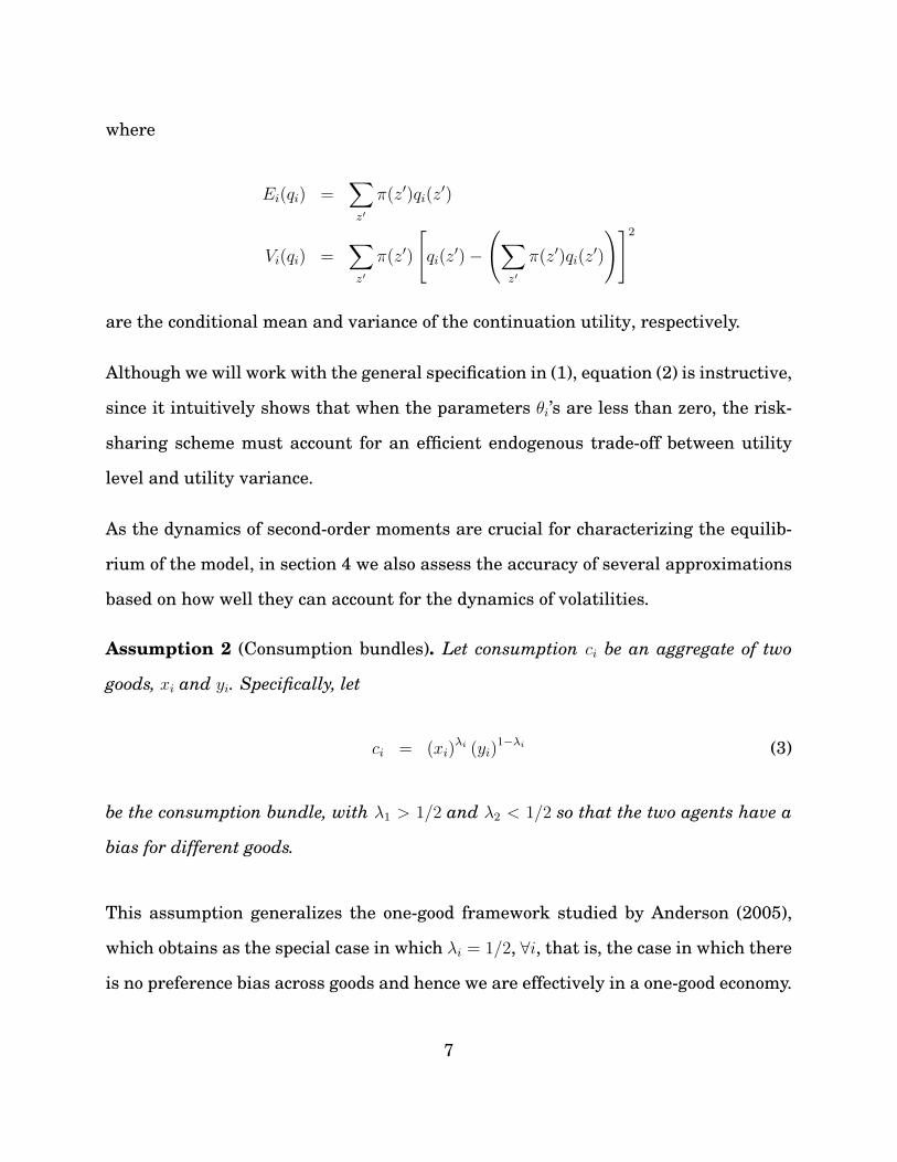
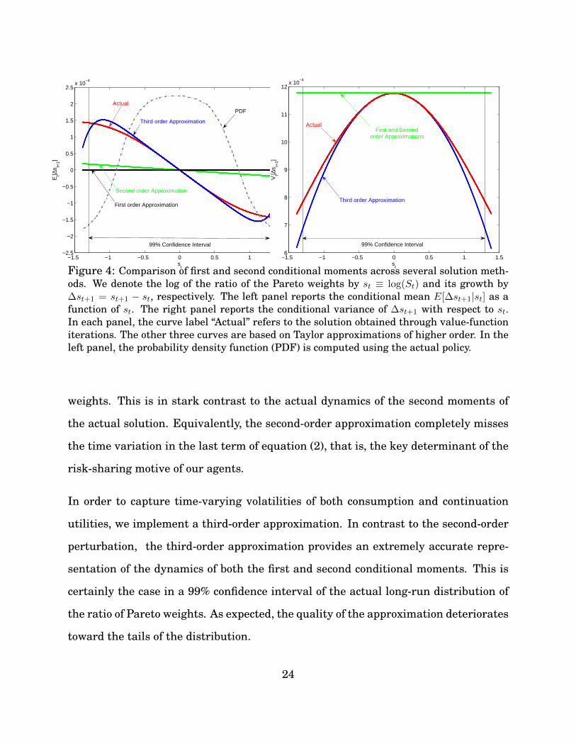
Figure 4: Comparison of first and second conditional moments across several solution meth-ods. We denote the log of the ratio of the Pareto weights by st ≡ log(St) and its growth by∆st+1 = st+1 − st, respectively. The left panel reports the conditional mean E[∆st+1|st] as afunction of st. The right panel reports the conditional variance of ∆st+1 with respect to st.In each panel, the curve label “Actual” refers to the solution obtained through value-functioniterations. The other three curves are based on Taylor approximations of higher order. In theleft panel, the probability density function (PDF) is computed using the actual policy.

weights. This is in stark contrast to the actual dynamics of the second moments of

the actual solution. Equivalently, the second-order approximation completely misses

the time variation in the last term of equation (2), that is, the key determinant of the

risk-sharing motive of our agents.

In order to capture time-varying volatilities of both consumption and continuation

utilities, we implement a third-order approximation. In contrast to the second-order

perturbation, the third-order approximation provides an extremely accurate repre-

sentation of the dynamics of both the first and second conditional moments. This is

certainly the case in a 99% confidence interval of the actual long-run distribution of

the ratio of Pareto weights. As expected, the quality of the approximation deteriorates

toward the tails of the distribution.

24

To summarize, this class of models produces rich dynamics for both the first and

second conditional moments of the Pareto weights and, therefore, consumption shares

across agents. To appropriately capture these dynamics, an approximation of at least

the third order is required. In the next section, we use third-order approximations to

study more general settings.

5 More General Environments

In this section we generalize our setting in two respects. First of all, we consider

preferences defined as in Epstein and Zin (1989),

Ui,t =

[(1− δ) · (Ci,t)1−1/ψ + δEt

[(Ui,t+1)1−γ] 1−1/ψ

1−γ

] 11−1/ψ

, ∀i ∈ 1, 2 , (14)

where ψ denotes the IES and γ represents RRA. Second, we consider the following

endowment process that allows persistence:

logXt = µ+ ρ logXt−1 − τ [logXt−1 − log Yt−1] + εXt (15)

log Yt = µ+ ρ log Yt−1 + τ [logXt−1 − log Yt−1] + εYt εXt

εYt

∼ iidN

0

0

, σX2 ρX,Y σ

XσY

ρX,Y σXσY σY 2

, (16)

where ρ ∈ [0, 1] and τ ∈ (0, 1) determine the extent of cointegration when ρ = 1.

Cointegration is required to have a well-defined ergodic distribution of the relative

supply of the two goods, but it plays a minor quantitative role in our analysis as we

set it to a very small number.

25

Solving the planner’s problem with global methods and multiple exogenous state vari-

ables goes beyond the scope of this manuscript. The reason is that properly capturing

the mean reversion of the pseudo-Pareto weights requires a very thin grid, and it

exposes us to the curse of dimensionality even with one extra state. Hence in this

section we explore the generality of our results through simulations based on a third-

order perturbation of our dynamic model, which we detail in Appendix D.

Reference calibration. Our reference calibration features µ = 2%, ρ = 0.90, σX =

σY = 1.87%, ρX,Y = 0.35, τ = 5.0E − 04, γ = 5, ψ = 1, δ = 0.96, and λ1 = λ2 = 0.97. The

parameters for the endowment processes are set in the spirit of Colacito and Croce

(2013). In what follows, we first consider different endowment processes and different

levels of the IES and RRA while preserving symmetry across agents and goods. We

then explore the implications for a small degree of heterogeneity in preference for the

two goods (λi) and in fundamental volatility across goods (σX and σY ).

5.1 Symmetric environments

The role of persistence. We vary the persistence of our endowment shocks from

zero to one. When ρ = 0, we have i.i.d. level shocks, as in the previous section. When

ρ = 1, level shocks are permanent. We depict key features of the distribution of the

log-ratio of the Pareto weights, st, in figure 5 and simulated moments in table 1.

We make several observations. First, as we increase ρ, the endowment shocks become

more long-lasting and volatile. As a result, the endogenous process st becomes more

volatile, as documented by its fatter tails (rightmost plot of figure 5, panel A) and the

26

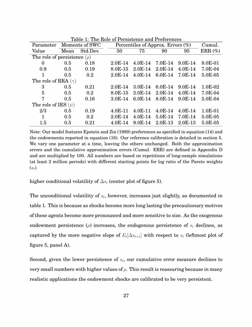
Table 1: The Role of Persistence and PreferencesParameter Moments of SWC Percentiles of Approx. Errors (%) Cumul.Value Mean Std.Dev. 50 75 90 95 ERR (%)The role of persistence (ρ)

0 0.5 0.18 2.0E-14 4.0E-14 7.0E-14 9.0E-14 8.0E-010.9 0.5 0.19 8.0E-15 2.0E-14 2.0E-14 4.0E-14 7.0E-041 0.5 0.2 2.0E-14 4.0E-14 6.0E-14 7.0E-14 5.0E-05

The role of RRA (γ)3 0.5 0.21 2.0E-14 3.0E-14 6.0E-14 9.0E-14 1.0E-025 0.5 0.2 8.0E-15 2.0E-14 2.0E-14 4.0E-14 7.0E-047 0.5 0.16 3.0E-14 6.0E-14 8.0E-14 9.0E-14 5.0E-04

The role of IES (ψ)2/3 0.5 0.19 4.0E-11 4.0E-11 4.0E-14 4.0E-14 1.0E-011 0.5 0.2 2.0E-14 4.0E-14 5.0E-14 7.0E-14 5.0E-05

1.5 0.5 0.21 4.0E-14 9.0E-14 2.0E-13 2.0E-13 5.0E-05

Note: Our model features Epstein and Zin (1989) preferences as specified in equation (14) andthe endowments reported in equation (16). Our reference calibration is detailed in section 5.We vary one parameter at a time, leaving the others unchanged. Both the approximationerrors and the cumulative approximation errors (Cumul. ERR) are defined in Appendix Dand are multiplied by 100. All numbers are based on repetitions of long-sample simulations(at least 2 million periods) with different starting points for log ratio of the Pareto weights(st).

higher conditional volatility of ∆st (center plot of figure 5).

The unconditional volatility of st, however, increases just slightly, as documented in

table 1. This is because as shocks become more long lasting the precautionary motives

of these agents become more pronounced and more sensitive to size. As the exogenous

endowment persistence (ρ) increases, the endogenous persistence of st declines, as

captured by the more negative slope of Et[∆st+1] with respect to st (leftmost plot of

figure 5, panel A).

Second, given the lower persistence of st, our cumulative error measure declines to

very small numbers with higher values of ρ. This result is reassuring because in many

realistic applications the endowment shocks are calibrated to be very persistent.

27

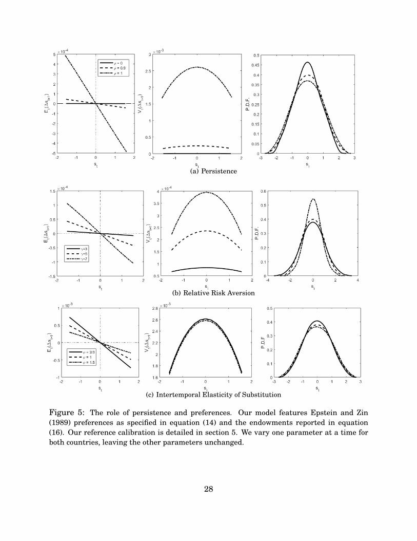
(a) Persistence

(b) Relative Risk Aversion

(c) Intertemporal Elasticity of Substitution

Figure 5: The role of persistence and preferences. Our model features Epstein and Zin(1989) preferences as specified in equation (14) and the endowments reported in equation(16). Our reference calibration is detailed in section 5. We vary one parameter at a time forboth countries, leaving the other parameters unchanged.

28

The role of preferences. When we vary the subjective discount factor, we do not

find significant changes in the dynamics of the log-ratio of the Pareto weights. For this

reason, we focus only on the role of risk aversion and IES. Increasing risk aversion

amplifies the sensitivity of continuation utility to shocks, and hence it makes the

redistribution channel stronger. This intuition is confirmed in panel (b) of figure 5,

where we show that the conditional variation of ∆st+1 increases with higher values of

γ and, at the same time, the mean reversion of the Pareto weights speeds up.

Since the endogenous change in mean reversion dominates quantitatively, as γ in-

creases more mass is concentrated in the center of the probability distribution func-

tion of st, implying that the unconditional volatility of this process declines. Together,

the faster speed of mean reversion and the lower unconditional volatility of st imply

lower levels of approximation errors.

We conclude this analysis by examining the case in which we vary the IES. The effect

of this parameter on the conditional volatility of the ratio of Pareto weights is almost

negligible (center plot of panel (c), figure 5). The impact on the endogenous persis-

tence of st is a bit more pronounced, but still moderate compared to the case in which

we change risk aversion. Qualitatively, agents with a higher IES are more willing

to accept fluctuations of consumption over time and hence are more willing to accept

very long-lasting reallocations, that is, slower mean reversion in st (leftmost plot in

panel (c), figure 5). Most importantly, we note that in the long-run risk literature the

IES is set to values larger than or equal to one. For these values, the approximation

errors are small, meaning that when the curvature of the utility function with respect

to intertemporal aggregation is moderate (ψ ≥ 1), the quality of our approximation is

good.

29

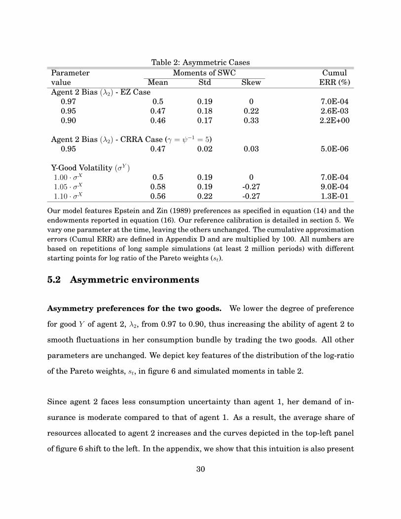
Table 2: Asymmetric CasesParameter Moments of SWC Cumulvalue Mean Std Skew ERR (%)Agent 2 Bias (λ2) - EZ Case

0.97 0.5 0.19 0 7.0E-040.95 0.47 0.18 0.22 2.6E-030.90 0.46 0.17 0.33 2.2E+00

Agent 2 Bias (λ2) - CRRA Case (γ = ψ−1 = 5)0.95 0.47 0.02 0.03 5.0E-06

Y-Good Volatility (σY )1.00 · σX 0.5 0.19 0 7.0E-041.05 · σX 0.58 0.19 -0.27 9.0E-041.10 · σX 0.56 0.22 -0.27 1.3E-01

Our model features Epstein and Zin (1989) preferences as specified in equation (14) and theendowments reported in equation (16). Our reference calibration is detailed in section 5. Wevary one parameter at the time, leaving the others unchanged. The cumulative approximationerrors (Cumul ERR) are defined in Appendix D and are multiplied by 100. All numbers arebased on repetitions of long sample simulations (at least 2 million periods) with differentstarting points for log ratio of the Pareto weights (st).

5.2 Asymmetric environments

Asymmetry preferences for the two goods. We lower the degree of preference

for good Y of agent 2, λ2, from 0.97 to 0.90, thus increasing the ability of agent 2 to

smooth fluctuations in her consumption bundle by trading the two goods. All other

parameters are unchanged. We depict key features of the distribution of the log-ratio

of the Pareto weights, st, in figure 6 and simulated moments in table 2.

Since agent 2 faces less consumption uncertainty than agent 1, her demand of in-

surance is moderate compared to that of agent 1. As a result, the average share of

resources allocated to agent 2 increases and the curves depicted in the top-left panel

of figure 6 shift to the left. In the appendix, we show that this intuition is also present

30

(a) Asymmetries in the degree of preference for the two goods

(b) Asymmetries in the degree of preference for the two goods - CRRA versus EZ

(c) Asymmetries in volatilities

Figure 6: Asymmetric calibrations. Our model features Epstein and Zin (1989) preferencesas specified in equation (14) and the endowments reported in equation (16). Our referencecalibration is detailed in section 5. We vary one parameter at a time, leaving the othersunchanged.

in the simple two-period model (see figure AF-1).

We note that the distribution of the log-ratio of the Pareto weights does not shift to the

left in a parallel way. As documented in the top portion of table 2, under the optimal

31

risk-sharing scheme, agent 1 accepts a lower average level of resources in exchange

for both a reduction in future utility uncertainty and positive skewness of its share of

world consumption. That is, agent 1 benefits from a sizeable positive redistribution

of resources along histories with a severe downside of the relative supply of good X.

Rabitsch, Stepanchuk and Tsyrennikov (2015) point out that a global approximation

is required when countries are subject to asymmetric constraints, such as a borrowing

limit, and when their wealth distribution is nonstationary. Since we have a friction-

less model with complete markets and a well-defined ergodic distribution of wealth, a

perturbation approach provides a good approximation of the equilibrium. Consistent

with the findings in Rabitsch et al. (2015), our cumulative errors increase as we make

the two agents more asymmetric, but our errors remain as low as 2.2%.

CRRA and heterogeneous degree of preference for the two goods. It is useful

to study this asymmetric scenario under time-additive CRRA preferences. We choose

the intermediate case λ1 = 0.97, λ2 = 0.95, and set ψ−1 = γ = 5.3 We fix the initial

ratio of the Pareto weights to a value that delivers an average SWC of 0.47, as in the

case with recursive preferences. Panel (b) of figure 6 and table 2 confirm that under

recursive preferences, the reallocation channel is very pronounced and long-lasting,

and it prescribes a significant amount of positive skewness for agent 1, as she is facing

more consumption risk because of a higher degree of preference for good X.

Heterogeneous volatility. In many applications, the properties of the goods traded

are asymmetric. In international finance, for example, different countries may be3Note that since γ > 1, the ratio of Pareto weights is no longer constant over time despite the

adoption of time additivity of preferences (Cole and Obstfeld (1991)). The implied variation in st,however, is very limited as highlighted in panel (b) of figure 6.

32

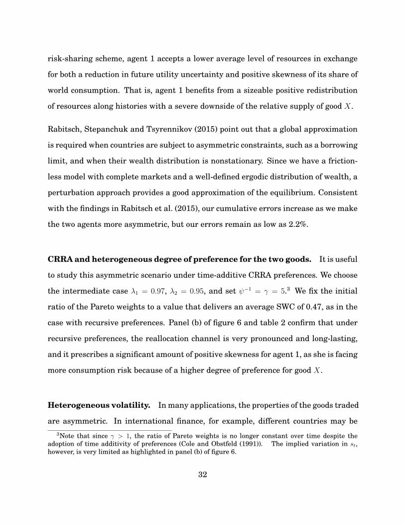
Figure 7: Asymmetric risk aversion. Our model features Epstein and Zin (1989) preferencesas specified in equation (14) and the endowments reported in equation (16). Our referencecalibration is detailed in section 5. We set γ2 = 7 and γ1 = 5 and vary simultaneously λ1 andλ2.

subject to productivity shocks with different volatilities. In the presence of the same

degree of preference for the two goods, the agent which prefers the more volatile good

faces more consumption and hence future utility uncertainty. As suggested by our

two-period model (see figure AF-1), this agent should be willing to accept a low av-

erage SWC in exchange for insurance. Panel (c) of figure 6 and table 2 confirm this

finding as we increase σY .

In this case, the average share of resources of agent 1 increases. The volatility of the

SWC increases as well, as a direct result of the higher standard deviation of good

Y . Agent 1 is willing to insure agent 2 against downside risk, and agent 1 accepts

negative skewness in her own share of resources. Across all cases, the associated

cumulative approximation errors are smaller than 0.14%.

33

Heterogenous RRA. A well-known result with multiple agents with risk-sensitive

preferences in a one-good economy with growth is that only the agent with the lowest

risk aversion remains wealthy in the long run, ceteris paribus (see Anderson (2005)).

We confirm this finding in our setting by depicting in figure 7 the expected growth

rate of the log-ratio of Pareto weights for the case λ1 = λ2 and γ2 > γ1. Since the

expected growth is positive for all values of st, all resources are allocated to agent 1

in the limit.

Our risk-sharing mechanism, however, suggests that as we make the degree of pref-

erence for the two goods more asymmetric, size matters progressively more for the

intensity of the reallocation channel. Hence as the high-risk-aversion agent receives

a smaller share of world resources, her willingness to buy further insurance should

decline, which in turn results in survivorship. Our simulations confirm this intuition

and suggest that there exist regions of the parameter space in which survivorship is

also possible with asymmetric risk aversion, provided that multiple parameters are

simultaneously adjusted, in the spirit of Anderson (2005).

6 Concluding Remarks

We have characterized the solution of a planner’s problem with multiple agents, mul-

tiple goods, and recursive preferences. The introduction of multiple goods substan-

tially changes the dynamics of Pareto optimal allocations. Future research should ex-

tend our theoretical results to continuous time and continuous shocks. Asset pricing

implications may be particularly appealing, due to the ability of this class of models to

endogenously produce time-varying second moments without requiring market fric-

34

tions. Since the main features of the risk-sharing scheme can be accurately captured

through a third-order approximation, this class of models could be easily extended to

an international business cycle setting as well.

35

References

Anderson, Evan W., “The dynamics of risk-sensitive allocations,” Journal of Economic The-

ory, 2005, 125(2), 93–150.

Anderson, E.W., L.P. Hansen, and T.J. Sargent, “Small Noise Methods for Risk-

Sensitive/Robust Economies,” Journal of Economic Dynamics and Control, 2012, 36(4),

468–500.

Backus, David, Chase Coleman, Axelle Ferriere, and Spencer Lyon, “Pareto weights

as wedges in two-country models,” Journal of Economic Dynamics and Control, 2016, 72

(Supplement C), 98 – 110.

Backus, David K., Bryan R. Routledge, and Stanley E. Zin, “Exotic Preferences for

Macroeconomists,” NBER Macroeconomics Annual 2004, 2005, 19, 319–414.

, , and , “Who holds risky assets?,” Working Paper, 2009.

Baker, Steven D. and Bryan R. Routledge, “The Price of Oil Risk,” Carnegie Mellon Uni-

versity and University of Virginia, Working Paper, 2017.

Bansal, Ravi and Amir Yaron, “Risks for the Long Run: A Potential Resolution of Asset

Pricing Puzzles,” Journal of Finance, 2004, 59, 1481–1509.

, Dana Kiku, Ivan Shaliastovich, and Amir Yaron, “Volatility, the Macroeconomy

and Asset prices,” Journal of Finance, 2014, 69(6), 2471–2511.

Borovicka, Jaroslav, “Survival and long-run dynamics with heterogeneous beliefs under

recursive preferences,” NYU, Working Paper, 2016.

Colacito, Riccardo and Mariano Croce, “International Asset Pricing with Recursive Pref-

erences,” Journal of Finance, 2013, 68(6), 2651–2686.

36

and Mariano M. Croce, “International Robust Disagreement,” American Economic

Review, 2012, 102(3), 152–55.

, Eric Ghysels, Jinghan Meng, and Wasin Siwarasit, “Skewness in Expected Macro

Fundamentals and the Predictability of Equity Returns: Evidence and Theory,” The Re-

view of Financial Studies, 2016, 20(8), 2069–2109.

Cole, H. and M. Obstfeld, “Commodity trade and international risk sharing. How much do

financial markets matter?,” Journal of Monetary Economics, 1991, 28, 3–24.

Duffie, D., P. Geoffard, and C. Skiadas, “Efficient and Equilibrium Allocations with

Stochastic Differential Utility,” Journal of Mathematical Economics, 1994, 23, 133–146.

Dumas, B., R. Uppal, and T. Wang, “The Global Stability of Efficient Intertemporal Alloca-

tions,” Journal of Economic Theory, 2000, 99, 240–259.

Epstein, L. G., “The Global Stability of Efficient Intertemporal Allocations,” Econometrica,

1987, 55, 329–355.

Epstein, Larry G. and Stanley E. Zin, “Substitution, Risk Aversion, and the Temporal

Behavior of Consumption and Asset Returns: A Theoretical Framework,” Econometrica,

1989, 57 (4), 937–969.

Geoffard, P. Y., “Discounting and Optimazing: Capital Accumulation as a Variational Min-

max Problem,” Journal of Economic Theory, 1996, 69, 53–70.

Hansen, L. and T. J. Sargent, “Discounted linear exponential quadratic gaussian control,”

IEEE Trans. Automatic Control, 1995, 40(5), 968–971.

and , Robustness, Princeton University Press, 2008.

Kan, R., “Structure of Pareto optima when agents have stochastic recursive preferences,”

Journal of Economic Theory, 1995, 66 (2), 626–31.

37

Kubler, Felix and Karl Schmedders, “Financial Innovation and Asset Price Volatility,”

American Economic Review, 2012, 102(3), 147–51.

Kuehn, Lars-Alexander and Oliver Boguth, “Consumption Volatility Risk,” Journal of

Finance, 2013, 68(6), 2589–2615.

Lucas, Robert and Nancy Stokey, “Optimal Growth with many consumers,” Journal of

Economic Theory, 1984, 32, 139–171.

Ma, Chenghu, “Market equilibrium with heterogenous recursive-utility-maximizing agents,”

Economic Theory, 1993, 7.

, “Corrigendum: Market Equilibrium with Heterogeneous Recursive-Utility-Maximizing

Agents,” Economic Theory, 1996, 3, 243–266.

Pohl, Walter, Karl Schmedders, and Ole Wilms, “Higher-Order Effects in Asset Pricing

Models with Long-Run Risks,” Working Paper, 2016.

Rabitsch, K., S. Stepanchuk, and Viktor Tsyrennikov, “International Portfolios: A Com-

parison of Solution Methods,” Journal of International Economics, 2015.

Sciubba, Emanuela, “Asymmetric information and survival in financial markets,” Economic

Theory, 2005, 25 (2), 353–379.

Segal, Gill, Ivan Shaliastovich, and Amir Yaron, “Good and Bad Uncertainty: Macroe-

conomic and Financial Market Implications,” Journal of Financial Economics, 2015,

117(2), 369–397.

Tallarini, Thomas, “Risk-Sensitive Real Business Cycles,” Journal of Monetary Economics,

2000, 45, 507–532.

Tretvoll, Hakon, “Real exchange rate variability in a two-country business cycle model,” BI

Norwegian Business School, Working Paper, 2016.

38

Tsyrennikov, Viktor, “Heterogeneous Beliefs, Wealth Distribution, and Asset Markets with

Risk of Default,” American Economic Review, 2012, 102(3), 156–60.

39

Appendix A. Two-Period Model.

Environment. In this section, we present a simplified two-period version of our model

in order to provide intuition on the reallocation motives induced by recursive preferences.

Specifically, at time t = 1 agents receive news ξ about their time-1 endowment of goods. At

time t = 0, that is, before the arrival of the shock, agents i ∈ 1, 2 exchange a complete set of

ξ-contingent securities to maximize their time-0 utility, given their initial wealth (reflected in

their time-0 Pareto weights).

Utility and technology. In what follows, we take advantage of lognormality wherever

possible. Up to a log linearization of the allocation shares, this modeling strategy enables us

to obtain a simple closed-form solution. In this spirit, we start by assuming that agents have

an IES equal to 1, that is, their preferences can be expressed as follows:

ui0 =

δθi logE0

[exp

ui1θi

]0 > θi > −∞

δE0[ui1] θi → −∞(A.1)

where

ui1 = log(Ci1)

and

C11 =

(X1

1

)λ1(Y 1

1

)(1−λ1), C2

1 =(X2

1

)(1−λ2) (Y 2

1

)λ2 . (A.2)

The resource constraints are specified as follows:

X11 +X2

1 = eξ, Y 11 + Y 2

1 = e−lξ, ξ ∼ N(0, σ2), (A.3)

where the parameter l determines whether agent 2 is more (l > 1) or less (0 < l < 1) exposed

to the shock ξ than agent 1. We assume that ξ affects both goods to preserve symmetry in our

40

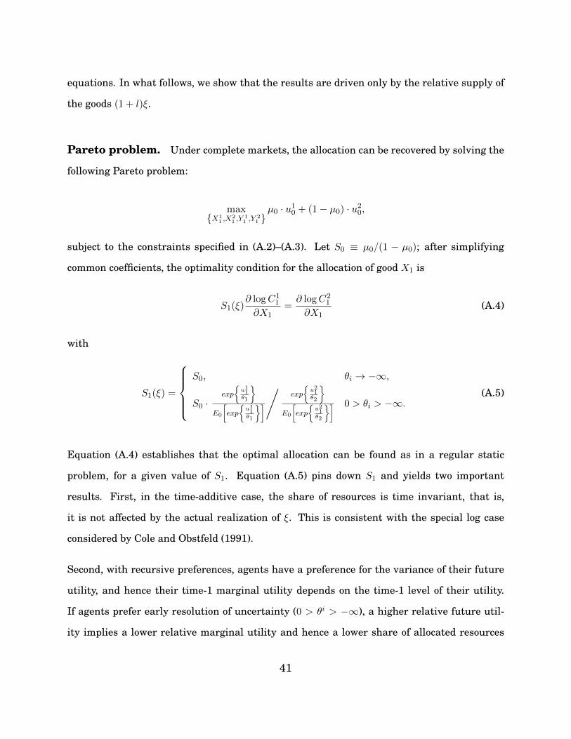
equations. In what follows, we show that the results are driven only by the relative supply of

the goods (1 + l)ξ.

Pareto problem. Under complete markets, the allocation can be recovered by solving the

following Pareto problem:

maxX1

1 ,X21 ,Y

11 ,Y

21 µ0 · u1

0 + (1− µ0) · u20,

subject to the constraints specified in (A.2)–(A.3). Let S0 ≡ µ0/(1 − µ0); after simplifying

common coefficients, the optimality condition for the allocation of good X1 is

S1(ξ)∂ logC1

1

∂X1=∂ logC2

1

∂X1(A.4)

with

S1(ξ) =

S0, θi → −∞,

S0 ·exp

u1

1θ1

E0

[exp

u1

1θ1

]/

exp

u2

1θ2

E0

[exp

u2

1θ2

] 0 > θi > −∞.(A.5)

Equation (A.4) establishes that the optimal allocation can be found as in a regular static

problem, for a given value of S1. Equation (A.5) pins down S1 and yields two important

results. First, in the time-additive case, the share of resources is time invariant, that is,

it is not affected by the actual realization of ξ. This is consistent with the special log case

considered by Cole and Obstfeld (1991).

Second, with recursive preferences, agents have a preference for the variance of their future

utility, and hence their time-1 marginal utility depends on the time-1 level of their utility.

If agents prefer early resolution of uncertainty (0 > θi > −∞), a higher relative future util-

ity implies a lower relative marginal utility and hence a lower share of allocated resources

41

(u11(ξ) > u2

1(ξ) → S1(ξ) < S0). Because of the dependence of S1 on future utility levels,

u11(ξ)− u2

1(ξ), the shock ξ prompts a reallocation at time 1.

Approximate solution. Define λ11−λ2

= κ1 and λ21−λ1

= κ2. At time 1, ξ is known and the

optimal allocations are

X11 =

S1κ1

1 + S1κ1eξ, X2

1 =1

1 + S1κ1eξ

and

Y1 =S1κ2

1 + S1κ2

e−lξ, Y 21 =

1

1 + S1κ2

e−lξ.

Since the allocations are a nonlinear function of S1(ξ), we log linearize them with respect to

s ≡ logS1 around s = s0 and obtain

log

(κ1e

s

1 + κ1es

)= log

(κ1e

s

1 + κ1es

)+

1

1 + κ1es(s− s)

log

(1

1 + κ1es

)= log

(1

1 + κ1es

)− κ1e

s

1 + κ1es(s− s)

log

(es

κ2

1 + es

κ2

)= log

(es

κ2

1 + es

κ2

)+

1

1 + es

κ2

(s− s)

log

(1

1 + es

κ2

)= log

(1

1 + es

κ2

)−

es

κ2

1 + es

κ2

(s− s)

and hence

logC11 = λ1

[log

(κ1e

s

1 + κ1es

)+

1

1 + κ1es(s− s) + ξ

]+ (1− λ1)

[log

(es

κ2

1 + es

κ2

)+

1

1 + es

κ2

(s− s)− lξ

]

logC21 = (1− λ2)

[log

(1

1 + κ1es

)− κ1e

s

1 + κ1es(s− s) + ξ

]+ λ2

[log

(1

1 + es

κ2

)−

es

κ2

1 + es

κ2

(s− s)− lξ

].

42

We can now write

u11 = logC1

1 = u11 + λξ

u11ξ (A.6)

u21 = logC2

1 = u21 + λξ

u21ξ, (A.7)

where

λξu1

1≡

[λ1

1 + κ1es+

1− λ1

1 + es

κ2

]λξs + λ1 − l + λ1l (A.8)

λξu2

1≡

[−(1− λ2)

κ1es

1 + κ1es− λ2

es

κ2

1 + es

κ2

]λξs + (1− λ2)− λ2l,

and

s− s = const(s) + λξs · ξ.

The elasticity λξs can be found taking into account equation (A.5):

λξs =λξu1

1

θ1−λξu2

1

θ2. (A.9)

Specifically, by combining equations (A.8)–(A.9), we have

λξs =1θ1

[(1 + l)λ1 − l] + 1θ2

[(1 + l)λ2 − 1]

1− 1θ1

[λ1

1+κ1es+ 1−λ1

1+ es

κ2

]− 1

θ2

[(1− λ2) κ1es

1+κ1es+ λ2

es

κ2

1+ es

κ2

] (A.10)

The constant can be recovered again from equation (A.5) accounting for second-order terms:

const(s) =1

2σ2

λξu21

θ2

2

−

λξu11

θ1

2 . (A.11)

43

Decentralization. Let the budget constraints of agent 1 and agent 2 be

X11 + p · Y 1

1 +

∫ξQ(ξ)A1

2(ξ) = eξ +A11,

X21 + p · Y 2

1 +

∫ξQ(ξ)A2

2(ξ) = e−lξ +A21,

where p is the price of good Y relative to good X, Q(ξ) is the price of an Arrow-Debreu security

that pays one unit of good X (the numeraire) contingent on the realization of ξ at date 2, and

Aji are the holdings of such security of agent j at date i. By market clearing, A1i + A2

i = 0,

∀i ∈ 1, 2.

Define ξ as the specific value of the state in which there is no reallocation effect, that is, s = s.

Under our approximation,

ξ = −const(s)λξs

.

This value is an important threshold for the portfolio allocation of our two agents in the com-

panion decentralized economy. In particular, at time 0, agent 1 buys Arrow-Debreu securities

paying a positive payoff for ξ < ξ, and sells Arrow-Debreu securities paying when ξ > ξ.

Since these assets are available in zero net supply, the exact opposite holds for agent 2. The

probability of agent 1 receiving a positive transfer is F (ξ), where F denotes the cumulative

distribution function of ξ. When ξ > 0, agent 1 has a higher probability of being a net receiver

of resources than agent 2.

Special cases. In the special case in which both agents have the same risk-sensitivity

parameter, θ1 = θ2 = θ, and the same exposure to the underlying shock, l = 1, we obtain

λξs =2θ (λ1 + λ2 − 1)

1− 1θ

[λ1

1+κ1es+ 1−λ1

1+ es

κ2

+ (1− λ2) κ1es

1+κ1es+ λ2

es

κ2

1+ es

κ2

] (A.12)

44

and λξs < 0 if θ < −∞ and λ1 + λ2 > 1, i.e., the ratio of the pseudo-Pareto weights is ‘coun-

tercyclical’, meaning that a smaller share of resources is assigned to agent 1 when there is

relative abundance of good 1. In this case,

const(s) =σ2

2θ2

[(λξu2

1)2 − (λξ

u11)2]. (A.13)

Let us also assume that λ1 = λ2 = λ > 1/2. In this case, we can derive the following results:

lims→−∞

λξs = 4(2λ− 1)

θ< 0 (A.14)

lims→−∞

const(s) =σ2

2θ2λξs

[λξs − 2(2λ− 1)

]> 0 (A.15)

lims→−∞

ξ = (2λ− 1)σ2

θ(θ − 1)> 0. (A.16)

Let F (ξ) be the cumulative distribution function of ξ. Conditional on s→ −∞, the probability

of country 1 to receive a higher share of resources in period 1 is F (ξ), and hence it increases

with (i) a stronger degree of preference for one of the two goods (λ), (ii) larger fundamental

risk (σ2), and (iii) stronger risk sensitivity (θ).

Figure AF-1, depicts const(s) (defined in equation A.11) as a function of s in two scenarios

with asymmetric calibrations.

45

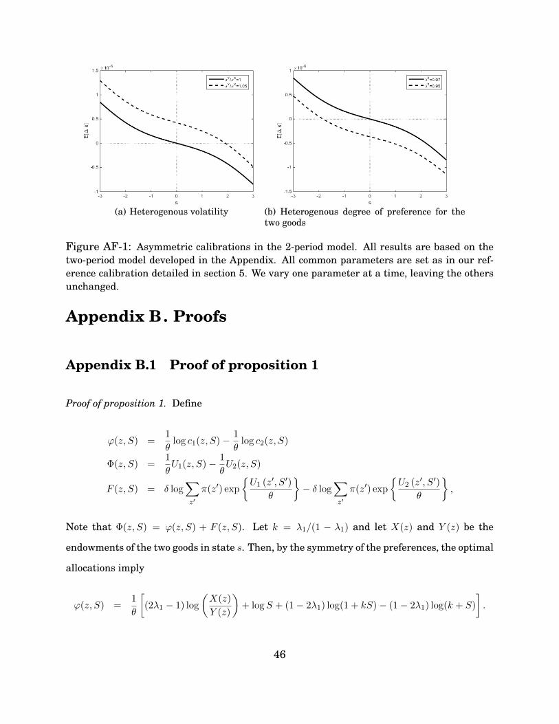
(a) Heterogenous volatility (b) Heterogenous degree of preference for thetwo goods

Figure AF-1: Asymmetric calibrations in the 2-period model. All results are based on thetwo-period model developed in the Appendix. All common parameters are set as in our ref-erence calibration detailed in section 5. We vary one parameter at a time, leaving the othersunchanged.

Appendix B. Proofs

Appendix B.1 Proof of proposition 1

Proof of proposition 1. Define

ϕ(z, S) =1

θlog c1(z, S)− 1

θlog c2(z, S)

Φ(z, S) =1

θU1(z, S)− 1

θU2(z, S)

F (z, S) = δ log∑z′

π(z′) exp

U1 (z′, S′)

θ

− δ log

∑z′

π(z′) exp

U2 (z′, S′)

θ

,

Note that Φ(z, S) = ϕ(z, S) + F (z, S). Let k = λ1/(1 − λ1) and let X(z) and Y (z) be the

endowments of the two goods in state s. Then, by the symmetry of the preferences, the optimal

allocations imply

ϕ(z, S) =1

θ

[(2λ1 − 1) log

(X(z)

Y (z)

)+ logS + (1− 2λ1) log(1 + kS)− (1− 2λ1) log(k + S)

].

46

Since θ < 0, if λ1 > 1/2 it follows that ϕ(z, S) is always: 1) decreasing in X(z)/Y (z) and 2) de-

creasing in S. Furthermore, F (s, S) is decreasing in S, since U1(z, S) (U2(z, S)) is increasing

(decreasing) in S, by the optimality of the social planner problem. Therefore, it has to be the

case that Φ(z, S) is decreasing in S.

Take two states, a and b, such that X ′(a)/Y ′(a) < X ′(b)/Y ′(b), and let S′a = fS(a, S) and

S′b = fS(b, S) be their respective ratios of Pareto weights. It is possible to characterize the

ratio:

S′bS′a

= exp

Φ(b, S′b

)− Φ

(a, S′a

).

Since Φ (z, S) is decreasing in z holding S fixed, it follows that exp Φ (b, S′a)− Φ (a, S′a) < 1.

Hence, if X ′(a)/Y ′(a) < X ′(b)/Y ′(b), it is never optimal to set S′a = S′b.

Additionally, the fact that Φ(s, S) is decreasing in S implies that

1 > exp Φ (b, S′a)− Φ (a, S′a) > Φ (b, S′b)− Φ (a, S′a) .

It follows that S′b < S′a.

Appendix B.2 Proof of proposition 2

We proceed in steps to provide a proof to roposition 2. Specifically, we state and prove four

propositions, which, combined, yield the proof of proposition 2. Throughout our exposition of

these propositions, we utilize the example proposed in main text, in order to better illustrate

the content of each statement.

We start by stating the following decomposition of the Pareto weights, the proof for which

follows directly from Anderson (2005). The rest of this section will consist of propositions

47

aimed at signing the covariance that appears on the right-hand side of this decomposition.

This will enable us to establish the relevant properties concerning the ergodicity and mean

reversion of the distribution of Pareto weights.

Proposition A4. The ratio of Pareto weights can be decomposed as

E[S′|S

]= S − cov [exp U ′2/θ , S′|S]

E [exp U ′2/θ |S], (B.17)

where E [S′|S] denotes the expectation of S′ conditional on s being the current state, and

cov[exp

U ′2/θ

, S′|S

]denotes the covariance between exp U ′2/θ and S′ conditional on the current S.

Proof. See Anderson (2005).

The next proposition draws a sharp contrast between a representative-agent economy and

our setting with multiple agents and goods. In a representative-agent economy, the consumer

enjoys a higher utility in the states of the world in which the supply of the most-preferred

good is more abundant. In the two agent economy that we consider in this paper, for any two

symmetric states there exists a finite ratio of Pareto weights below which the ranking of the

future utility functions across states is reversed.

Proposition A5. For any two symmetric states zi and z−i, such that X(zi) > Y (zi), there exists

a finite Si1 < 1 such that U1

(zi, fS

(zi, S

i1

))= U1

(z−i, fS

(z−i, S

i1

)), where fS (·, ·) is defined in

(10), and U1

(zi, fS

(zi, S

i1

))< U1

(z−i, fS

(z−i, S

i1

)), ∀Si1 < Si1.

Proof. Let S′i = fS(zi, S) and S′−i = fS(z−i, S) be the ratios of Pareto weights when tomorrow’s

symmetric states are zi and z−i, respectively. Using equation (9), the ratio between S′i and S′−i

48

isS′iS′−i

= exp

U1 (z′i, S

′i)− U1

(z′−i, S

′−i)

θ

/exp

U2 (z′i, S

′i)− U2

(z′−i, S

′−i)

θ

.

Rearranging, we have

U1

(z′i, S

′i

)− U1

(z′−i, S

′−i)

= U2

(s′i, S

′i

)− U2

(z′−i, S

′−i)

+ θ[logS′i − logS′−i]. (B.18)

We shall characterize the limit of the left-hand side of equation (B.18) for µ1 that tends to

zero. First, notice that consumption bias (λ1 > 1/2) implies that

limµ1→0

U2

(z′i, S

′i

)− U2

(z′−i, S

′−i)< 0. (B.19)

Then, notice that equation (C.35) and the fact that the planner’s problem is twice continuously

differentiable imply the continuity of the fS function with respect to S. Also, at µ1 = 0,

S′i = S′−i = 0. Hence

limµ1→0

S′i = S′i∣∣µ1=0

= S′−i∣∣µ1=0

= limµ1→0

S′−i,

which implies that

limµ1→0

log(S′i − logS′−i

)= 0. (B.20)

Combining (B.19) and (B.20) into (B.18), we obtain that

limµ1→0

U1

(z′i, S

′i

)− U1

(z′−i, S

′−i)< 0. (B.21)

Since λ1 > 1/2, it follows that

limµ1→1 U1 (zi, S′)− U1 (z−i, S

′) > 0. (B.22)

49

Combining (B.21) and (B.22) concludes the proof.

Corollary 1. For any two symmetric states zi and z−i, such that X(zi) > Y (zi), there exists a

finite Si2 > 1 such that U2

(zi, fS

(zi, S

i2

))= U2

(z−i, fS

(z−i, S

i2

)), where fS (·, ·) is defined in

(10), and U2

(zi, fS

(zi, S

i2

))> U2

(z−i, fS

(z−i, S

i2

)), ∀Si2 > Si2.

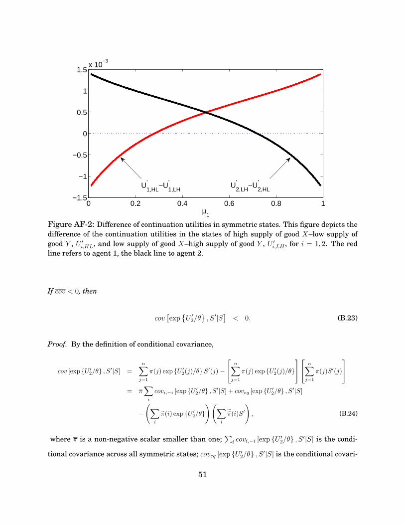
We illustrate the content of the preceding proposition and corollary in figure AF-2, which

depicts the differences of the continuation utilities in the two states of unequal supply of the

two goods for the example discussed in section 3.2 of the main text.

When the Pareto weight attached to agent 1 (agent 2) is approaching 1, the continuation

utility for the state of abundant supply of good X (good Y ) is higher than the continuation

utility for the state of scarce supply of good X. However, as suggested by proposition A5,

there exists a µ1 < 1/2 (1 − µ1 < 1/2) past which the ranking of the continuation utilities is

reversed.

We are now ready to characterize the sign of the covariance term in (B.17). The following

definition of conditional covariance in symmetric states is useful in establishing an upper

bound on the last term of equation (B.17).

Definition 2 (Covariance of symmetric states). Let zi, z−i ∈ N be symmetric states. The

conditional covariance between two random variables h and g valued on zi, z−i is

covi,−i [h, g|S] =∑

l=i,−i

p(zl)h(zl)g(zl)−

∑l=i,−i

p(zl)h(zl)

∑l=i,−i

p(zl)g(l)

,

where p(zl) ≡ π(zl)/(π(zi) + π(z−i)).

Proposition A6. Let cov be the sum of the conditional covariances between exp U ′2/θ and S′

across all symmetric states:

cov =∑i

covi,−i[exp

U ′2/θ

, S′|S

].

50

0 0.2 0.4 0.6 0.8 1−1.5

−1

−0.5

0

0.5

1

1.5x 10

−3

µ1

U1,HL’ −U

1,LH’ U

2,LH’ −U

2,HL’

Figure AF-2: Difference of continuation utilities in symmetric states. This figure depicts thedifference of the continuation utilities in the states of high supply of good X–low supply ofgood Y , U ′i,HL, and low supply of good X–high supply of good Y , U ′i,LH , for i = 1, 2. The redline refers to agent 1, the black line to agent 2.

If cov < 0, then

cov[exp

U ′2/θ

, S′|S

]< 0. (B.23)

Proof. By the definition of conditional covariance,

cov [exp U ′2/θ , S′|S] =

n∑j=1

π(j) exp U ′2(j)/θS′(j)−

n∑j=1

π(j) exp U ′2(j)/θ

n∑j=1

π(j)S′(j)

= π

∑i

covi,−i [exp U ′2/θ , S′|S] + coveq [exp U ′2/θ , S′|S]

−

(∑i

π(i) exp U ′2/θ

)(∑i

˜π(i)S′

), (B.24)

where π is a non-negative scalar smaller than one;∑

i covi,−i [exp U ′2/θ , S′|S] is the condi-

tional covariance across all symmetric states; coveq [exp U ′2/θ , S′|S] is the conditional covari-

51

ance across all states of equal supply; and π(i)ni=1 and˜π(i)

ni=1

are non-negative sequences

of scalars.

We know from proposition 1 that the optimal choice of Pareto weights is identical across all

states in which the supply of the two goods is the same. This implies that

coveq[exp

U ′2/θ

, S′|S

]= 0.

We can also conclude that the last term in equation B.24 is non-negative, being the product of

the sums of non-negative terms.

Therefore, we can state that

cov[exp

U ′2/θ

, S′|S

]≤ π

∑i

covi,−i[exp

U ′2/θ

, S′|S

],

which concludes the proof.

The sign of cov is key. Suppose that the current ratio of Pareto weights is in the region

between zero and miniSi2 as defined in corollary 1. For any two symmetric states, the utility

of agent 2 is going to be larger when the supply of good Y is relatively more abundant. Since

the parameter θ is negative, the ranking of U2/θ is reversed. Proposition 1 suggests that

the ratio of Pareto weights is larger when the supply of good Y is larger. Therefore we can

conclude that, in this region, cov, and hence the covariance term in (B.17), are negative. This

argument is summarized in figure AF-3.

The next proposition plays a crucial role in our proof for the existence of a well-defined ergodic

distribution of the Pareto weights. We focus on the properties of the left tail of the stochastic

process S′ = µ′11−µ′1

= fS(z′, S) and base our proof on all the other propositions developed so far.

Proposition A7. The stochastic process S (S) := min(S,miniSi2

), where Si2 is defined as in

52

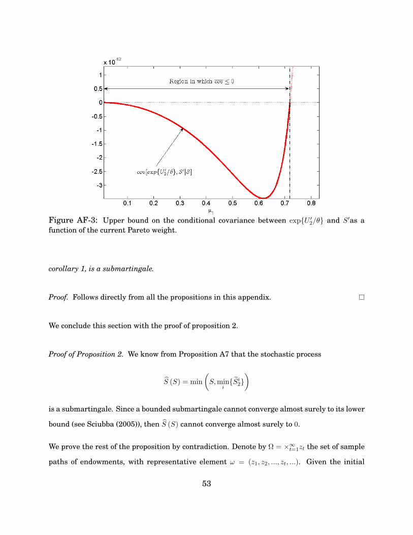
Figure AF-3: Upper bound on the conditional covariance between expU ′2/θ and S′as afunction of the current Pareto weight.

corollary 1, is a submartingale.

Proof. Follows directly from all the propositions in this appendix.

We conclude this section with the proof of proposition 2.

Proof of Proposition 2. We know from Proposition A7 that the stochastic process

S (S) = min

(S,min

iSi2

)

is a submartingale. Since a bounded submartingale cannot converge almost surely to its lower

bound (see Sciubba (2005)), then S (S) cannot converge almost surely to 0.

We prove the rest of the proposition by contradiction. Denote by Ω = ×∞t=1zt the set of sample

paths of endowments, with representative element ω = (z1, z2, ..., zt, ...). Given the initial

53

Pareto weight ratio S0 = 1 and the transition dynamics S′ = fS(z′, S), the ratio of Pareto

weights at time t can be written as a function of the sample path: St = St(ω).

Suppose Proposition 2 does not hold. Then, there must exist a set of ω such that

Prω| lim

t→∞St(ω) = 0

> 0 (B.25)

Denote by Q = ω| limt→∞

St(ω) = 0 and consider the natural filtration on Q: Q1 ⊆ Q2 ⊆ ... ⊆

Qt ⊆ ... ⊆ Q. Recall that zt∞t=1 is i.i.d. As in Sciubba (2005), Qt−1 does not restrict the

original probability distribution of zt, and hence we have that Przt = z(i)|Qt−1 = π(z(i)). As

a consequence, all the results that we have proved so far in this section apply with respect to

the conditioning set Qt−1. This means that St is a bounded submartingale with respect to the

conditioning information set Qt−1. Since a bounded submartingale cannot converge almost

surely to its lower bound, then St cannot converge almost surely to 0 on Q. This contradicts

the definition of Q. Hence, St cannot converge to 0 with probability 1. Equivalently, the

probability that St converges to 0 is null.

Note that µ1

(S)

= S

1+S, that is, µ1

(S)

is a non-negative, monotonically increasing function

of S. It follows that µ1 cannot also converge to 0 almost surely. By repeating all the proofs in

the paper for µ2 = 1 − µ1, it follows by symmetry that µ2 cannot converge to 0 almost surely.

Equivalently, µ1 cannot converge to 1 almost surely either.

Appendix B.3 Proof of proposition 3

This section reports the proof of the proposition on the mean-reversion property of the Pareto

weight.

Proof of proposition 3. We prove the three statements in proposition 3 in the same order in

54

which they appear in the proposition’s claim.

1. We show that only µ1 = 1/2 is such that E [µ′1|S] = µ1.

After imposing a symmetrical calibration, the recursive definition of the ratio of Pareto

weights derived in the paper becomes

µ′11− µ′1

=µ1

1− µ1· exp U1 (z′, S′) /θ∑

z′ π(z′) exp U1 (z′, S′) /θ

∑z′ π(z′) exp U2 (z′, S′) /θ

exp U2 (z′, S′) /θ.

By rearranging and taking the conditional expectation operator, we obtain

E [µ′1|S] = µ1 − µ1 ·cov [µ′1, exp U ′1/θ |S]

E [exp U ′1/θ |S]− (1− µ1) · cov [µ′1, exp U ′2/θ |S]

E [exp U ′2/θ |S]. (B.26)

For each µ1 = µ∗1 such that E [µ′1|S] = µ∗1, equation (B.26) implies that

µ∗1 =cov [µ′1, exp U ′2/θ |S]

E [exp U ′2/θ |S]

/(cov [µ′1, exp U ′2/θ |S]

E [exp U ′2/θ |S]− cov [µ′1, exp U ′1/θ |S]

E [exp U ′1/θ |S]

). (B.27)

By symmetry, for each µ∗1 < 1/2, there must exist a µ∗∗1 = 1−µ∗1 such that E [µ′1|S] = µ∗∗1 .

At µ∗∗1 = 1− µ∗1, equation (B.26) implies that

µ∗1 =cov [µ′1, exp U ′1/θ |S]

E [exp U ′1/θ |S]

/(cov [µ′1, exp U ′1/θ |S]

E [exp U ′1/θ |S]− cov [µ′1, exp U ′2/θ |S]

E [exp U ′2/θ |S]

). (B.28)

Combining equations (B.27) and (B.28), we obtain that at µ∗1 the following condition

must hold:

cov [µ′1, exp U ′1/θ |S]

E [exp U ′1/θ |S]= −cov [µ′1, exp U ′2/θ |S]

E [exp U ′2/θ |S]. (B.29)

By plugging condition (B.29) into equation (B.27) or (B.28), we conclude that the only

µ∗1 ∈ (0, 1) such that E [µ′1|S] = µ∗1 is µ∗1 = 1/2.

2. We show that if µ1 > 1/2, then E [µ′1|S] < µ1.

We know from proposition A7 that the stochastic process S (S) = min(S,miniSi2

),

where miniS2 > 1 is a submartingale. Since, by definition, S (S) =µ1(S)

1−µ1(S), and

55

the stochastic process µ1 cannot converge to 1 (see proposition 2), there must exist a

µ+1 >

mini Si2

1+mini Si2> 1/2 such that E [S′|S+] = S+, where S+ =

µ+1

1−µ+1

. Since S = µ1

1−µ1is a

convex function in µ1,

µ+1

1− µ+1

= E[S′|S+

]= E

[µ′1

1− µ′1

∣∣∣∣S+

]= cov

[µ′1,

1

1− µ′1

∣∣∣∣S+

]+ E

[µ′1|S+

]E

[1

1− µ′1

∣∣∣∣S+

]>= cov

[µ′1,

1

1− µ′1

∣∣∣∣S+

]+ E

[µ′1|S+

] 1

1− E [µ′1|S+].

Since µ′1 and 11−µ′1

are both monotonically increasing functions of µ′1, cov[µ′1,

11−µ′1

∣∣∣S+]>

0. This implies that

µ+1

1− µ+1

>= cov

[µ′1,

1

1− µ′1

∣∣∣∣S+

]+ E

[µ′1|S+

] 1

1− E [µ′1|S+]

> E[µ′1|S+

] 1

1− E [µ′1|S+]

from which we obtain

E[µ′1|S+

]< µ+

1 .

Since we know that there exists only one µ∗1 = 1/2 such that E[µ′1|

µ∗11−µ∗1

]= µ∗1, by the

continuity of fS with respect to S, it must be the case that E [µ′1|S] < µ1, ∀µ1 ∈ (1/2, 1).

3. We show that if µ1 < 1/2, then E [µ′1|S] > µ1.

This proof mirrors the one that we just provided for µ1 > 1/2, and thus for parsimony

we omit it here.

56

Appendix C. Recursive Method and Global Solution

Given the conditions in Ma (1993) and Ma (1996), the social planner’s value function, denoted

as Qp(z, µ1) : N × [0, 1]→ R, satisfies the following functional equation proposed by Lucas and

Stokey (1984), and Kan (1995):

Qp(z, µ1) = maxxi,yi,qi,z′i∈1,2,z′∈N

2∑i=1

µi logW ∗i (z, ci, qi,z′z′) (C.30)

subject to

µ2 = 1− µ1

0 ≤ x1 ≤ X(z), 0 ≤ x2 ≤ X(z)− x1

0 ≤ y1 ≤ Y (z), 0 ≤ y2 ≤ Y (z)− y1

ci = (xi)λi (yi)

1−λi , ∀i = 1, 2

0 ≤ minµ1(z′)∈[0,1]

Qp(z′, µ1(z′))− µ1(z′)q1,z′ − (1− µ1(z′))q2,z′ ∀z′ ∈ N (C.31)

Remark Appendix C.1. Let assumption (1)–(4) hold. When µi = 0, interpret µi logW ∗i (z, ci, qi,z′z′) =

0. Since 0 < X(z) < ∞ and 0 < Y (z) < ∞, ∀z ∈ N , it can be proved that there exists a unique

bounded and continuous solution to (C.30)–(C.31). A feasible allocation is Pareto optimal if

and only if it is generated recursively from the solution to (C.30)–(C.31).

Assumptions (1)–(4) are sufficient to apply the contraction mapping theorem to the planner’s

problem described by the system of equations (4)-(5). This result is parallel to those proposed

by Lucas and Stokey (1984), Kan (1995) and Anderson (2005).

IES=1: a two-step approach. It is convenient to use the definition of risk sensitive prefer-

ences in equation (1) to notice that the recursive planner’s problem can be decomposed in two

57

parts:

Qp(s, µ1) = QAp (s, µ1) +QBp (s, µ1)

where QAp (s, µ1) is the static social planning problem

QAp (s, µ1) ≡ maxxi≥0,yi≥0i∈1,2

µ1(1− δ1) log c1 + (1− µ1)(1− δ2) log c2 (C.32)

subject to:

X(z) ≥ x1 + x2, Y (z) ≥ y1 + y2,

ci = (xi)λi(yi)

1−λi i = 1, 2;

and QBp (s, µ1) is related to the allocation of future utilities

QBp (z, µ1) ≡ maxDz′

µ1δ1 log

[∑z′

exp(1− γ1)(q2,z′ +Dz′)πs

]+ (C.33)

(1− µ1)δ2 log

[∑z′

exp(1− γ2)q2,z′πs

]

subject to

q2,z′ = Qp

(z′,

dQpdµ1

−1

(z′, Dz′)

)−Dz′

dQpdµ1

−1

(z′, Dz′) ∀z′ ∈ N , (C.34)

where Dz′ is defined as the difference of the future utilities in state z′: Dz′ ≡ q1,z′−q2,z′ . Equa-

tion (C.34) defines the Pareto frontier and is obtained using equations (5)–(7). By equation (7),

the first derivative of Qp is strictly increasing, hence, invertible. Equation (6) implies that:

µ1(z) =dQpdµ1

−1

(z, q1,z − q2,z). (C.35)

58

Appendix D. Allocation as a Function of Pareto Weights

Let W it = W (Cit , U

it+1) be the right-hand side of equation (14). If we denote the partial deriva-

tives of the aggregator W i as

W i1,t :=

∂W it

∂Cit, W i

2,t :=∂W i

t

∂U it+1

,

then the stochastic discount factor is equal to

M it+1 =

W i2,tW

i1,t+1

W i1,t

∀i = 1, 2. (D.36)

The optimality condition for the allocation of good Xt for t = 1, 2, ... in each possible state is

µh0 ·

t−1∏j=0

W 12,j

·W 11,tC

1t

λ1

x1t

=(1− λ2)

x2t

C2tW

21,t ·

t−1∏j=0

W 22,j

· µ20. (D.37)

Define the date t Pareto weights as

µit = µi0 ·

t−1∏j=0

W i2,j

·W i1,tC

it

= µit−1 ·W i2,t−1 ·

W i1,t

W i1,t−1

· CitCit−1

= µit−1 ·M it · exp

∆cit

, ∀i ∈ h, f.

It follows that equation (D.37) can be rewritten as

µ1t ·λ1

x1t

=(1− λ2)

x2t

· µ2t . (D.38)

59

Let St := µ1t /µ

2t . Then the optimality condition in equation (D.38) can be represented by the

following system of recursive equations:

Stλ1

x1t

=(1− λ2)

x2t

St = St−1M1t e

∆c1t

M2t e

∆c2t, (D.39)

where

Mi,t+1 = δ

(Ci,t+1

Ci,t

)− 1ψ

U1−γi,t+1

Et

[U1−γi,t+1

]

1/ψ−γ1−γ

. (D.40)

A similar first-order condition applies with respect to good Y .

Approximation methods and errors. We use perturbation methods to solve our system of

equations and compute our policy functions using the dynare++4.2.1 package. All variables

are expressed in log-units.

In tables 1 and 2, we report statistics regarding the maximum cumulative approximation

error (Cumul. ERR) for our relative pseudo-Pareto weights, that is, the key drivers of both

consumption shares. The maximum is taken across agents, and we account for the fact that

the relative Pareto weights are persistent and errors can accumulate over longer simulations.

More specifically, we construct recursively the following processes:

Sj,t = Sj,t−1 ·Mj,t

M1,t

·

(Cj,t/Cj,t−1

C1,t/C1,t−1

), ∀t ≥ 1, (D.41)

where we adopt the “·” notation to indicate approximated variables. We initialize the recursion

at different starting points, Sj,0 and we then define the error for agent j as follows:

errjt =1

t

t∑τ=1

∣∣∣∣∣ Sj,τSj,τ− 1

∣∣∣∣∣ · 100.

60

Sj is the approximated relative pseudo-Pareto weight that we obtain directly from our pertur-

bation method. Sj is constructed by dynamically updating our equilibrium recursion (i.e.,

an exact dynamic equation) for Sj,t using our approximated forcing elements, Mj,t, M1,t,

Cj,t/Cj,t−1, and C1,t/C1,t−1. Examination of the discrepancy between Sj and Sj constitutes

a valid metric for assessing the quality of the approximation, as this discrepancy accounts for

the persistent impact that the errors on our forcing terms can have on the relative pseudo-

Pareto weights.

We also show percentiles of the one-period-ahead errors, which tend to be many orders of

magnitude smaller. Across all cases, the approximation errors are small and comparable to

those obtained under regular time-additive preferences and thus are negligible for all practi-

cal purposes.

61