23 11

Article 13.5.3Journal of Integer Sequences, Vol. 16 (2013),2

3

6

1

47

Recursive Bijections for Catalan Objects

Stefan ForceyDepartment of MathematicsThe University of AkronAkron, OH 44325-4002

USAsf34@uakron.edu

Mohammadmehdi Kafashan and Mehdi MalekiDepartment of Electrical Engineering

The University of AkronAkron, OH 44325-4002

USA

Michael StrayerDepartment of MathematicsThe University of AkronAkron, OH 44325-4002

USA

Abstract

In this note we introduce several instructive examples of bijections found between

several different combinatorially defined sequences of sets. Each sequence has cardi-

nalities given by the Catalan numbers. Our results answer some questions posed by R.

Stanley in the addendum to his textbook. We actually discuss two types of bijection,

one defined recursively and the other defined in a more local, relative, fashion. It is

interesting to compare the results of the two.

1

1 Introduction

1.1 Catalan objects

In the work that led to this note we set out to find explicit bijections between severalsequences of sets that are known to be counted by the Catalan numbers, sequence A000108in [6]. One sequence of sets we call the right-swept planar unary-binary trees, or right-swepttrees for short. These are the same restriction of planar unary-binary trees that are labeledas example “www” in R. Stanley’s Catalan Addendum (version of July 2012) [5]. In [3] Kimdescribes what we call right-swept trees as a special kind of planar unary-binary trees, andKim gives in the same article a bijection to the non-crossing partitions. We were inspired tofind bijections from these right-swept trees to other familiar sets of objects counted by theCatalan numbers, due to the fact that they have a nice recursive description that is differentfrom the standard Catalan recursion. In this paper we find bijections from the right-swepttrees to staircase tilings, planar trees, planar binary trees and arc tree diagrams, allowingthe reader to construct many more implied bijections to non-crossing partitions, polygonaldissections and lattice paths. Our first set of recursive bijections is described in Section 2.Our second bijection between staircase tilings and right-swept trees is discussed in Section 3.

A right-swept tree is a rooted planar tree with the following restrictions. In general anode may be a leaf, may have a single child which must be left, middle, or right; or insteadmay have two children: left and right. Any left child has further restrictions: it may notbe a leaf, and it may not have a middle child. Thus any branching to the left is eventuallyswept right before it can end in a leaf. Figure 1 shows a right-swept tree.

Figure 1: Two views of a right-swept tree. We will use the first, with root at the top. The(remixed) photo is a windswept hawthorne near Galway, original taken by Eoin Gardiner(creative commons).

Our second featured sequence is known as the diagonal rectangular tilings of staircase

shapes, or staircase tilings for short. A staircase shape is the outline of a Young diagramcorresponding to a partition given by (n, n − 1, . . . , 1). The Catalan numbers count tilingswhose rectangles each include some of the stepped diagonal – i.e., each intersects the end of arow in the Young diagram. These are equivalently described as rectangular tilings of height

2

n staircase shapes that contain exactly n rectangles. The fact that having n rectangles isequivalent to being a diagonal tiling is also true for diagonal rectangulations of the square,and we refer the reader to [4] both for a proof and for some very nice related combinatorics.The staircase tilings are also referred to as tilings of stair-step shapes, as in [2].

There is a well known bijection from staircase tilings to the sets of rooted planar binarytrees. Simply removing the “steps,” the vertical and horizontal boundary segments of unitlength at the far right and bottom of the figure, and adding a root, yields a binary tree(whose drawing has been rotated from its normal presentation.) A staircase tiling and itscorresponding binary tree is shown in Figure 2.

Figure 2: Two views of a staircase tiling. We will use the version on the left. The binarytree in the center is the image of the staircase tiling under the classical bijection: it is formedby removing the steps. We will draw rooted binary trees with the root at the bottom.

The bijection exemplified in Figure 2 is trivially described in recursive terms. A planarbinary tree t with more than one leaf (and thus the corresponding staircase tiling) is formedby joining a pair of smaller binary trees–the left and right subtrees whose root is the firstbranch point of t. Many other Catalan objects have a similar recursive description–triangulardissections of a polygon, bracketings of a string of symbols, and Dyck paths, to name a few.This description leads to Segner’s classic recursion relation for the Catalan numbers cn:

c0 = 1 and cn+1 =n∑

k=0

ckcn−k for n > 0, (1)

where n is the number of branch points for the binary tree, or the number of rectangles inthe staircase tiling. The recursion yields the closed formula:

cn =1

n+ 1

(

2n

n

)

.

If Xn and X ′

n are any two of the sequences of sets that have Segner’s recursive descriptionthen they are in piecewise bijection (both counted by cn), and the correspondence is explicitlydescribed using the recursion. If a bijection is given between the kth sets of the two sequences,

3

for k = 1 . . . n, then given an object ofXn+1 we can decompose it into two objects from earlierin the sequence, find their corresponding objects and use them to construct the correspondingobject in X ′

n+1.

We began by using a different, nonstandard recursion for the Catalan numbers to seekbijections between the staircase tilings and the right-swept trees. Our first bijection discussedin Section 2 is based on an alternate recursive description of the staircase tilings, which fitswell with the natural recursive description of the right-swept trees. Here is the recursionthat we will be using (its four parts will be explained one at a time in Section 2):

cn+1 = cn + cn + (cn − cn−1) +

(

n−1∑

k=2

cn−k(ck − ck−1)

)

.

By finding analogous ways to recursively construct other sorts of Catalan objects we candescribe them as being in bijection with the right-swept trees, and each other, in new ways.As an example we include non-crossing arc diagrams with distinct left endpoints, or arc trees

for short.Arc trees are defined to be the ways of connecting n+1 points lying on a horizontal line

on the plane with n non-crossing arcs lying above the line such that the left endpoints ofthe arcs are distinct. There is always a unique series of arcs traveled from left to right fromany point to the rightmost point. Thus there is always a unique shortest path to travel fromone point to another. These are easily seen to be in bijection with planar rooted trees withn edges, simply by choosing the rightmost point to be the root and then straightening thearcs. See Figure 3.

Figure 3: The bijection from non-crossing arc diagrams with distinct left endpoints to planarrooted trees: from left to right we gradually straighten the arcs. We will draw planar rootedtrees with the root at the bottom (as opposed to the right-swept trees with their root at thetop.)

2 Recursive bijections

As mentioned, in order to keep this paper self contained, we have repeated the definitionsgiven in R. Stanley’s Catalan addendum (version of 13 July 2012) to [5] of the combinatorial

4

objects www, h8, and h5: called here, respectively, the right-swept trees, staircase tilingsand arc trees.

We represent the set of right-swept trees with n nodes as Tn, the set of stair-case tilingswith n rectangles as Sn and the set of arc trees with n arcs as An. We refer to the sets asthe shapes of size n. The five objects for size n = 3 are seen in Figures 4, 5 and 6.

Figure 4: Right-swept trees T3.

Figure 5: Staircase tilings S3.

Figure 6: (Non crossing) arc trees A3.

Here we introduce a recursive method to construct a shape with size of n + 1 in any ofthese three combinatorial sets using shapes of smaller size. We construct four different typesof shapes of size n+ 1 using four methods:

1. We define functions fR : Xn → Xn+1, X ∈ {T,S,A} , n ≥ 1 ∈ N. Depending onwhich combinatorial object is the input to this function, we perform the following pro-cedures:

a) X = T: In this case, the output in Tn+1 = fR (Tn) is a right-swept tree with n+ 1vertices constructed by adding one vertex to t ∈ Tn as the new root whose right childis the root of t.

5

b) X = S: In this case, the output in Sn+1 = fR (Sn) is a staircase tiling with n + 1rectangles constructed by adding one ((n+ 1)× 1) rectangle to the left side of an inputfrom Sn.

c) X = A: In this case, the output in An+1 = fR (An) is is an arc tree with n + 2points constructed by adding one point to the left side of a ∈ An and connecting it tothe nearest point in a.

Figure 7 represents the operation of fR whose input can be any possible shape withsize of n. Thus the number of shapes of size n + 1 which can be constructed by fR isdenoted cn+1,1 = cn.

T n

S n

An

Figure 7: Construction of Xn+1 using fR.

2. We define functions fM : Xn → Xn+1, X ∈ {T,S,A} , n ∈ N, and for the case n = 0.Depending on which combinatorial object is the input to this function, we perform thefollowing procedures:

a) X = T: In this case, the output in Tn+1 = fM (Tn) is a tree with n + 1 verticesconstructed by adding one vertex to t ∈ Tn as the new root whose middle child is theroot of t. We define T0 to be {∅} and define the single element of T1 as fM(∅).

b) X = S: In this case, the output in Sn+1 = fM (Sn) is a tiling with n+ 1 rectanglesconstructed by removing the left edge of s ∈ Sn, extending s one column to the leftand then adding one single square to the bottom of the new column. We define S0 tobe {∅} and define the single element of S1 as fM(∅).

c) X = A: In this case, the output in An+1 = fM (An) is an arc tree with n+2 pointsconstructed by adding one point to the left side of a ∈ An and connecting it to thefarthest point in a. We define A0 to consist of a single point and define the singleelement of A1 as the image of that point under fM .

Figures 8 and 9 represent the operation of fM whose input can be any possible shapewith size of n. Thus the number of shapes of size n + 1 which can be constructed by

6

fM is denoted cn+1,2 = cn.

T n

S n

An

Figure 8: Construction of Xn+1 using fM .

T 5 S 5

T 4 S 4

f fM M

A5

A4

fM

Figure 9: Examples of the construction of Xn+1 using fM .

3. We define functions fL : (Xn − fM(Xn−1)) → Xn+1, X ∈ {T,S,A} , n ≥ 1 ∈ N.Depending on which combinatorial object is the input to this function, we perform thefollowing procedures:

a) X = T: In this case, the output of fL is a tree with n + 1 vertices constructed byadding one vertex to a size n right-swept tree t as the new root whose left child is theroot of t. Here the original root of t will not have a middle child.

b) X = S: In this case, the output of fL is a tiling with n+1 rectangles constructed byadding one ((n+ 1)× 1) rectangle to the top of a shape from Sn. Here s ∈ Sn shouldnot have a single square as its lowest tile. In other words s should not be constructedby fM (Sn−1).

c) X = A: In this case, the output of fL is an arc tree with n + 2 points constructedby adding one point to the left side of a size n arc tree a and connecting it to the

7

second nearest point (but not the rightmost one) in a such that the connection doesnot intersect with any other arc in a. Notice that this is impossible if the input arc treehas an arc between its first and last points. In other words a should not be constructedby fM (An−1).

Figure 10 represents the operation of fL whose input can be any possible shape withsize of n except the shapes constructed by fM (Xn−1). Thus the number of shapes ofsize n+ 1 which can be constructed by fL is denoted cn+1,3 = cn − cn−1.

T n

S n

An

Figure 10: Construction of Xn+1 using fL.

4. For the last case we define functions f : ((Xn1− fM(Xn1−1))×Xn2

) → Xn+1, X ∈{T,S,A} , n1 > 1 ∈ N, n2 ∈ N, n = (n1+n2) ≥ 3. Depending on which combinatorialobject is the input to this function, we perform the following procedures:

a) X = T: In this case, the output in Tn1+n2+1 is a tree with n1 + n2 + 1 verticesconstructed by adding one vertex as the root whose left and right children are theroots of trees from Tn1

− fM(Tn1−1) and Tn2, respectively.

b) X = S: In this case, the output in Sn1+n2+1 is a shape with n1 + n2 + 1 rectanglesconstructed by introducing a rectangle of size ((n1 + 1)× (n2 + 1)) in the top left cor-ner of the shape and adding staircase tilings t1 ∈ Sn1

− fM(Sn1−1) and t2 ∈ Sn2to the

bottom and right of the rectangle, respectively. The tiling added to the bottom shouldnot have a single square as its bottom-most tile.

c)X = A: In this case, the output in An1+n2+1 is a shape with points constructed byconcatenating arc trees from An1

− fM(An1−1) and An2in that order, left to right, by

identifying their respective rightmost and leftmost points. Then we add a point to theleft side of both and connect it to the identified common point. The input arc tree onthe left should not have an arc between its first and last points.

Figure 11 represents the operation of f (., .) to construct a shape of size n1 + n2 + 1.The first input argument can be any shape with size of n1 > 1 except the shapes

8

constructed by fM (Xn1−1). However the second argument can be any shape of sizen2. The number of shapes of size n+ 1 which can be constructed with this function is

denoted cn+1,4 =n−1∑

k=2

cn−k (ck − ck−1).

Tn 1Tn 2 S n 1

S n 2

An 1An 2

Figure 11: Construction of Xn1+n2+1 using f (Xn1,Xn2

)

2.1 Bijections implied by the construction.

The functions we have defined allow the shapes to be built recursively, and to be decon-structed as well. Unique construction and deconstruction allow us to realize a bijectionbetween any two sets whose shapes are built with the four functions defined above. Firstwe note that there is only one element of X1 for each of the shapes we consider. Figure 12shows the three sets of size one.

Definition 1. For n ≥ 1 we define maps α : Xn → X′

n for X,X′ ∈ {T,S,A} as follows:For x ∈ Xn we consider x to be the shape that results from applying exactly n functions

fi, i = 1 . . . n in a particular order to k initial copies of x0 ∈ X0, the single element of size zerofor k ≥ 1. Here fi ∈ {f, fL, fR, fM}. We denote as Fx the function that is the compositionof cartesian products of the n functions fi, whose domain is k copies of X0, and whose soleimage is x.

Then α(x) = Fx(x′

0, x′

0, . . . , x′

0) for k copies of x′

0 ∈ X′

0, the element of size zero.

For examples see Figures 13, 15 and 16.

Theorem 2. α : Xn → X′

n as just defined gives bijections for all X,X′ ∈ {T,S,A}.

Proof. We show that α is well defined, surjective and invertible by demonstrating that forany shape x′ ∈ X′

n there is a unique composition of cartesian products of functions from

T 1 S 1 A1

Figure 12: Trivial bijections between T1, S1 and A1. Recall that these are each defined asan image of fM .

9

fL, fM , fR and f that constructs it. Since a given composition constructs only one shape ineach of T,S,A, having that composition means having knowledge of a unique shape x ∈ Xn

corresponding to x′. The existence of a unique composition is argued using strong induction,since the function f takes inputs from sets with smaller indices than just n−1. We note thatthe single shapes for n = 1 (in Figure 12) are all constructed uniquely by fM by definition.Assuming that shapes smaller than size n are uniquely constructed, we then check for sizen as follows:

T : For any right-swept tree t ∈ Tn, depending on whether the root has left, middle, rightor both left and right children, the tree is uniquely constructed from one or two smallertrees. For the right-swept trees this follows from their definition.

S : For any staircase tiling s ∈ Sn the shape is uniquely constructed from one or twosmaller shapes. The construction is determined first by whether s has a single squareas its bottom-most tile. If that is the case, then s is constructed from a single smallertiling by fM . Otherwise, we can determine whether it was constructed by fL, fR or f ,respectively, by whether s has a a single long rectangle along its top, along its left side,or neither (instead it has a thick rectangle that covers some of both but neither theentire top nor the entire left edges.)

A : For any arc tree a ∈ An the shape is constructed from one or two smaller shapes.The construction is determined first by whether a has a single arc connecting its firstand last points. If that is the case, then a is constructed from a single smaller arctree by fM . Otherwise, we can determine whether it was constructed by fR, fL or f ,respectively, by whether a has a a single short arc connecting its first (leftmost) andsecond points, a single arc connecting its left-most point with the second availablepoint, or neither (instead it has a single longer arc connecting its left-most point toanother, more central, point.)

It is instructive to show that the total number of shapes constructed by our four functions

is equal to cn+1. That is, that the Catalan number cn+1 =4∑

i=1

cn+1,i. Equivalently we need

to prove thatn−1∑

k=1

ckcn−k = cn+1 − 2cn. To see this we expanded the sum and used Segner’s

recurrence relation for Catalan numbers:

c0 = 1 and cn+1 =n∑

k=0

ckcn−k for n > 0. (2)

So we have

cn+1 =n∑

k=0

ckcn−k = c0cn +n−1∑

k=1

ckcn−k + cnc0 ⇒n−1∑

k=1

ckcn−k = cn+1 − 2cn. (3)

10

2.2 Examples

Example 1: We want to demonstrate the bijections between right-swept trees, staircasetilings and arc trees for n = 3. For this we use the proposed method twice. So for n = 2 thebijection between these combinatorial objects is illustrated in Figure 13:

T 2 S 2 A2

Figure 13: Bijections between right-swept trees, staircase tilings and arc trees for n = 2.The top row is formed by fM ◦ fM and the bottom row by fR ◦ fM .

Now the bijections between right-swept trees, staircase tilings and arc trees for n = 3 canbe illustrated, in Figure 18:

Example 2: Here we take a shape in S12, seen in Figure 14. We want to find its images underα in T12 and A12. First we apply the inverses of our functions introduced before in order to

Figure 14: An example of a staircase tiling with n = 12.

uniquely reduce the size of the shape to n = 1, shown in Figure 15. Now by applying thefunctions we found in Figure 15, we can construct bijective images of the staircase tiling inthe sets of right-swept trees and arc trees, which are shown in Figure 16. Finally we presentthe induced bijective correspondence for a binary tree with 12 internal nodes and a planartree with 12 edges. This is seen in Figure 17.

11

f-1

M

f-1

f-1

L

f-1

R

f-1

f-1

R

f-1

R

f-1

R

f-1

M

Figure 15: The inverse process on shape of Figure 14. Darkly shaded tiles are discarded bythe inverse functions. Thus the tiling x shown here is formed by

Fx(x0, x0, x0) = f(fM ◦ fL ◦ fR ◦ fM ◦ fM(x0), fR ◦ f(fM(x0), fR ◦ fR ◦ fM(x0))).

Figure 16: Images (under α) of the shape of Figure 14 in T12 and A12

3 Relative bijection from Tn to Sn

For contrast, we consider a different method for constructing a bijection from right-swepttrees to staircase tilings.

We start by describing a second new mapping β : Tn → Sn. Rather than using recursion,this time we declare several rules about the relative positions of rectangles on one hand andtree nodes on the other. To characterize this mapping, we need several rules which describehow two labeled nodes attached by an edge of the right-swept tree are translated to twolabeled rectangles in the staircase tiling.

1. Let two nodes be attached by a tree edge with a positive slope, so that node a is a leftchild of node b. Then rectangle b will be immediately to the right of rectangle a. SeeFigure 19.

12

Figure 17: Corresponding binary tree and planar tree, under bijection induced by α betweenarc trees and staircase tilings. This example uses the staircase tiling from Figure 14 andFigure 15.

right-swept

trees

staircase

tilingsarc

trees

(planar rooted)

binary trees

(planar rooted)

trees

f f f o o M M M

f f f o o R M M

f f f o o M R M

f f f o o R R M

f f f o o L R M

Figure 18: Bijections for n = 3. Each row represents a class of objects mapped to each other,the first three columns by the bijection α and the last two columns via canonical bijectionsfrom the staircase tilings and arc trees.

2. For two nodes attached by a negative sloped edge the situation is more complex. If aright child b is the only child of a root, middle child, or right child a, and b itself is a

13

Figure 19: Example of Rule 1 (β : Tn → Sn).

leaf or has only a middle or right child, then the rectangle b will be immediately rightof the rectangle corresponding to a. See Figure 20.

Figure 20: Example of Rule 2 (β : Tn → Sn).

3. However, if a right child is produced from a left child (or as part of a left and right child),the corresponding rectangle will be immediately below the rectangle corresponding tothe spawning vertex. See Figure 21.

Figure 21: Examples of Rule 3 (β : Tn → Sn). Rectangles labeled with a letter correspondto that node, as shown by the circles.

4. A middle child b will always correspond to a rectangle directly below the rectanglecorresponding to the spawning vertex a. See Figure 22.

14

Figure 22: Example of Rule 4 (β : Tn → Sn).

5. There is only one case in which adjacent nodes do not correspond to adjacent rectangles:if b is a right child of a, and b has a left child d. Then rectangle b is right of rectangle a,but Rule 1 is used to place the left child of b (and its left child, etc.) between rectanglesa and b. See Figure 23.

Figure 23: Example of Rule 5 (β : Tn → Sn). The three circled nodes b, d, c all correspondto rectangles right of the rectangle corresponding to a.

This method gives a specific set of instructions at each vertex point for how to proceedwith no ambiguity in the decision-making process. Therefore each tree in Tn will give aunique structure in Sn.

Figure 24 is a final example for the case that n = 10 for the mapping from Tn to Sn.

Theorem 3. The mapping β : Tn → Sn determined by the above rules is a bijection.

Proof. We consider the reverse mapping β−1 : Sn → Tn. In a similar fashion, we develop aseries of rules for this mapping.

1. If the top-left rectangle goes to the bottom of the figure (i.e., width = 1 unit), theroot spawns a right child. If the top-left rectangle goes to the farthest right edge (i.e.,depth = 1 unit), the root spawns a middle child. This process is repeated as necessary.See Figure 25.

2. If the top-left rectangle has width greater than 1 unit and depth greater than 1 unit,then a limb of left children is formed where the bottom vertex on this limb correspondsto the left-most rectangle. The length of this limb of left children is determined by the

15

Figure 24: A full example for the case n = 10 (β : Tn → Sn).

Figure 25: Examples of Rule 1 (β−1 : Sn → Tn).

Figure 26: Example of Rule 2 (β−1 : Sn → Tn).

number of rectangles read from left to right, going as far right as possible. See Figure26.

3. Any remaining rectangles are treated as right children of the vertex corresponding to

16

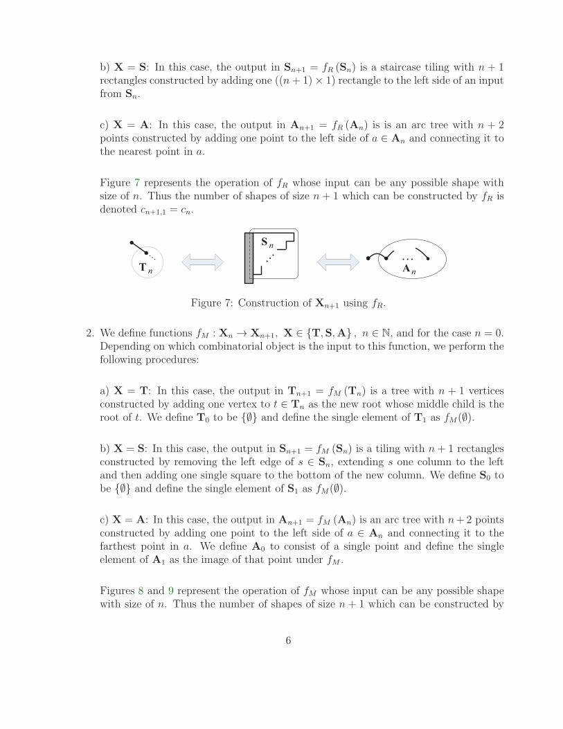
the rectangle directly above and the process repeats with these remaining rectanglesacting as miniature versions of Sn. Notice this rule satisfies the restriction in Tn tohave a right child or a right and left child following a left child. See Figure 27.

Figure 27: Example of Rule 3 (β−1 : Sn → Tn).

As in the previous case, we now illustrate with a final example, the reverse image for thecase n = 10 that we considered earlier. See Figure 28. We use the set of rules developedhere, and see that we arrive at the same pre-image in Tn.

Figure 28: A full example for the case n = 10 (β−1 : Sn → Tn).

Once again, no ambiguity arises from the rules developed above, and so each output ofthis algorithm is unique for each unique input.

We now argue that these sets of rules form an inverse function. We define Tier One rulesto be Rules 2 and 4 from the former direction and Rule 1 from the latter direction. Wedefine Tier Two rules to be Rules 1 and 5 in the former direction and Rule 2 in the latterdirection. We define Tier Three rules to be Rule 3 from the former direction and Rule 3from the latter direction.

Tier One rules are easily seen to be inverse rules, and when using any Tier One rule fromthe outset, the resulting figure in the next step is a new tree or staircase shape with n − 1vertices or rectangles for Tn and Sn, respectively.

17

The real key to this process occurs in Tier Two and Tier Three rules. In Tn, the TierTwo rules occur any time a left child is introduced, whether it is from the root (Rule 1) orsomewhere else in the tree (Rule 5). In Sn, the Tier Two rules occur any time a rectanglehaving width and depth both greater than 1 unit is introduced, either as the top-left rectangle(corresponding to the root in Tn) or somewhere else in the staircase (corresponding to adifferent branch in Tn). These two phases are clearly inverses of each other, since Rules 1and 5 of Tn imply Rule 2 of Sn and vice versa, and in corresponding sections of the tree andstaircase.

Tier Three rules in Tn occur whenever a right child branches off of a left limb (wherethe length of the limb is anywhere from 1 to n − 1 branches). Similarly, Tier Three rulesin Sn occur any time there are leftover rectangles underneath of a Tier Two structure inSn. In both Tn and Sn, the process renews itself when Tier Three rules are utilized, leavingsmaller tree and staircase structures of corresponding size, both starting independently withthe same set of rules the larger structure obeys. Therefore, Tier Three rules in Tn implyTier Three rules in Sn and vice verse, and in corresponding sections of the tree and staircase.

Breaking down our algorithm into three tiers of rules has allowed us to show that thisfunction is indeed an inverse function. We therefore have successfully described the bijectionbetween Sn and Tn.

3.1 Examples contrasting the bijections.

Interestingly, the two bijections α : Tn → Sn and β : Tn → Sn set up precisely the samecorrespondence between right-swept trees and staircase tilings for n = 0, 1, 2. An obviousquestion is raised: are the two bijections we have described the same? The answer is no. Wesee this at n = 3, by comparing the tables in Figures 29 and 18.

18

Figure 29: Bijections for n = 3 for the bijection β. Note that the third and fifth images areswitched from those of α in Figure 18.

The slightly larger example we include next in Figure 30 was suggested by an anonymousreferee, to whom we owe heartfelt thanks for catching early errors. This example is in n = 5.

αβ

Figure 30: Contrasted pre-images of an S5 tiling.

Finally we include here in Figure 31 a larger example to highlight the differences. A treefrom T12 (the same example as in Figure 16) is shown in the center, and then its two imagesin S12: on the left is the image of the recursive bijection from Section 2 and on the right theimage of the relative bijection from Section 3.

19

α

β

Figure 31: Two images of a right-swept tree from T12.

References

[1] R. P. Stanley, Enumerative Combinatorics, Vol. 2, Cambridge University Press, 1999.

[2] M. Crepinsek and L. Mernik, An efficient representation for solving Catalan numberrelated problems, Int. J. of Pure and Applied Math. 56 (2009), 589–604.

[3] J. S. Kim, Front representation of set partitions, SIAM J. Discrete Math. 25 (2011),447–461.

[4] S. Law and N. Reading, The Hopf algebra of diagonal rectangulations, J. Combin. Theory

Ser. A. 119 (2012), 788–824.

[5] R. P. Stanley, Enumerative Combinatorics, Vol. 2, Cambridge University Press, 1999.

[6] N. J. A. Sloane, The On-Line Encyclopedia of Integer Sequences, http://oeis.org/.

2010 Mathematics Subject Classification: Primary 05C05; Secondary 05A19.Keywords: Catalan numbers, bijection, recursion.

(Concerned with sequence A000108.)

Received December 1 2012; revised versions received February 24 2013; May 2 2013. Pub-lished in Journal of Integer Sequences, May 9 2013.

Return to Journal of Integer Sequences home page.

20