Reduced-Basis Methods Applied to Problems in Elasticity:

Analysis and Applications

by

Karen Veroy

S.M. Civil Engineering (2000)Massachusetts Institute of Technology

B.S. Physics (1996)Ateneo de Manila University, Philippines

Submitted to the Department of Civil and Environmental Engineeringin partial fulfillment of the requirements for the degree of

Doctor of Philosophy

at the

MASSACHUSETTS INSTITUTE OF TECHNOLOGY

June 2003

c© Massachusetts Institute of Technology 2003. All rights reserved.

Author . . . . . . . . . . . . . . . . . . . . . . . . . . . . . . . . . . . . . . . . . . . . . . . . . . . . . . . . . . . . . . . . . . . . . . . . . . . . . . . . . . .Department of Civil and Environmental Engineering

April 15, 2003

Certified by. . . . . . . . . . . . . . . . . . . . . . . . . . . . . . . . . . . . . . . . . . . . . . . . . . . . . . . . . . . . . . . . . . . . . . . . . . . . . . .Anthony T. Patera

Professor of Mechanical EngineeringThesis Supervisor

Certified by. . . . . . . . . . . . . . . . . . . . . . . . . . . . . . . . . . . . . . . . . . . . . . . . . . . . . . . . . . . . . . . . . . . . . . . . . . . . . . .Franz-Josef Ulm

Professor of Civil and Environmental EngineeringChairman, Thesis Committee

Accepted by . . . . . . . . . . . . . . . . . . . . . . . . . . . . . . . . . . . . . . . . . . . . . . . . . . . . . . . . . . . . . . . . . . . . . . . . . . . . . .Oral Buyukozturk

Professor of Civil and Environmental EngineeringChairman, Department Committee on Graduate Students

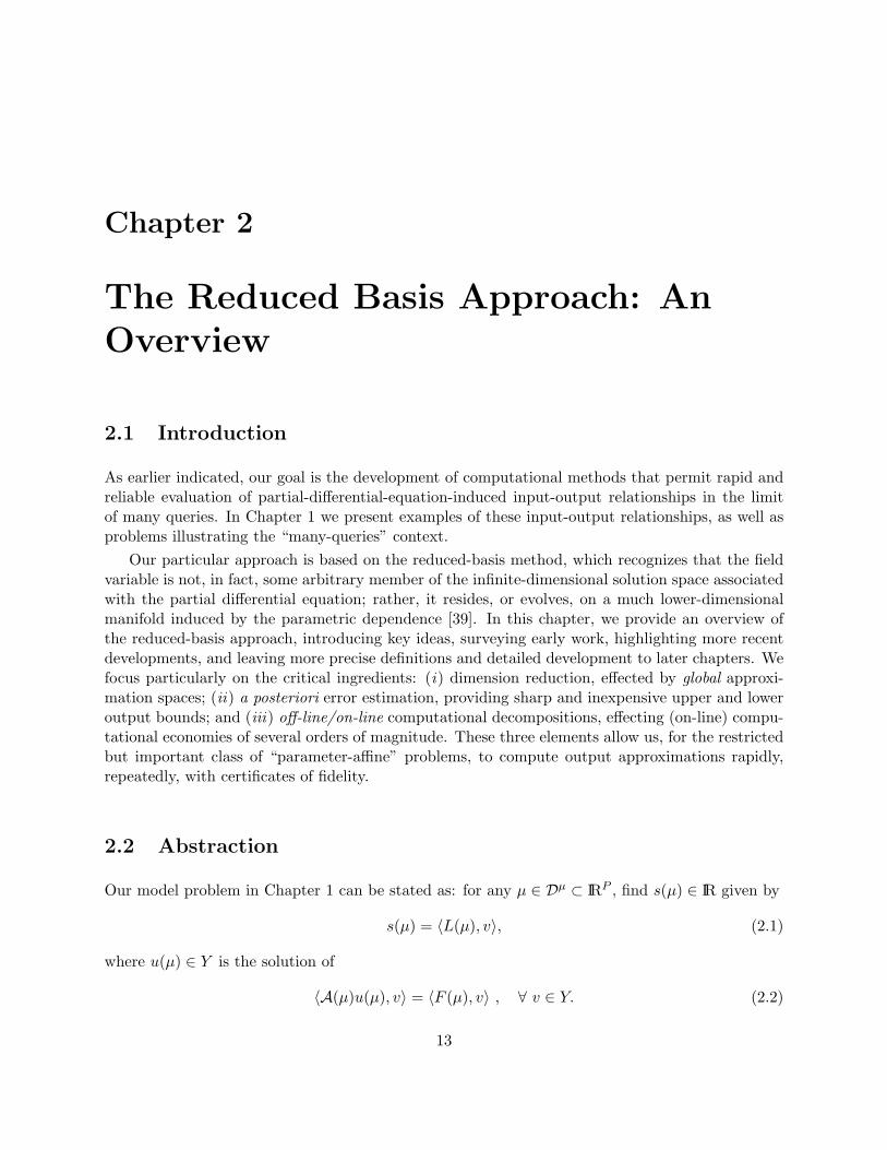
Reduced-Basis Methods Applied to Problems in Elasticity: Analysis andApplications

byKaren Veroy

Submitted to the Department of Civil and Environmental Engineeringon April 15, 2003, in partial fulfillment of the

requirements for the degree ofDoctor of Philosophy

Abstract

Modern engineering problems require accurate, reliable, and efficient evaluation of quantities ofinterest, the computation of which often requires solution of a partial differential equation. Wepresent a technique for the prediction of linear-functional outputs of elliptic partial differentialequations with affine parameter dependence. The essential components are: (i) rapidly convergentglobal reduced-basis approximations — projection onto a space WN spanned by solutions of thegoverning partial differential equation at N selected points in parameter space (Accuracy); (ii) aposteriori error estimation — relaxations of the error-residual equation that provide inexpensivebounds for the error in the outputs of interest (Reliability); and (iii) off-line/on-line computationalprocedures — methods which decouple the generation and projection stages of the approximationprocess (Efficiency). The operation count for the on-line stage depends only on N (typically verysmall) and the parametric complexity of the problem.

We present two general approaches for the construction of error bounds: Method I, rigorous aposteriori error estimation procedures which rely critically on the existence of a “bound conditioner”— in essence, an operator preconditioner that (a) satisfies an additional spectral “bound” require-ment, and (b) admits the reduced-basis off-line/on-line computational stratagem; and Method II,a posteriori error estimation procedures which rely only on the rapid convergence of the reduced-basis approximation, and provide simple, inexpensive error bounds, albeit at the loss of completecertainty. We illustrate and compare these approaches for several simple test problems in heatconduction, linear elasticity, and (for Method II) elastic stability.

Finally, we apply our methods to the “static” (at conception) and “adaptive” (in operation)design of a multifunctional microtruss channel structure. We repeatedly and rapidly evaluatebounds for the average deflection, average stress, and buckling load for different parameter valuesto best achieve the design objectives subject to performance constraints. The output estimatesare sharp — due to the rapid convergence of the reduced-basis approximation; the performanceconstraints are reliably satisfied — due to our a posteriori error estimation procedure; and thecomputation is essentially real-time — due to the off-line/on-line decomposition.

Thesis Supervisor: Anthony T. PateraTitle: Professor of Mechanical Engineering

Acknowledgments

I have had the most wonderful fortune of having Professor Anthony T. Patera as my advisor. Forhis support and guidance, his counsel and example, his humor and patience, I am truly grateful.

I would like to thank the members of my thesis committee, Professor Franz-Josef Ulm andProfessor Jerome J. Connor, and also Professor John W. Hutchinson of Harvard University andProfessor Anthony G. Evans of the University of California (Santa Barbara), for their comments,suggestions, and encouragement throughout my studies. I am very thankful to have had theopportunity to learn from and interact with them.

During my doctoral studies, I have had the good fortune to extensively collaborate with IvanOliveira, Christophe Prud’homme, Dimitrios Rovas, Shidrati Ali, and Thomas Leurent; this workwould not have been possible without them. I would also like to thank Yuri Solodukhov, NgocCuong Nguyen, Lorenzo Valdevit, and Gianluigi Rozza for many helpful and interesting discussions.Furthermore, I am most grateful to Debra Blanchard for her invaluable help and support, and forproviding almost all of the wonderful artwork in this thesis.

Finally, I owe the deepest gratitude to my family — Raoul, Lizza, Butch, Chesca, Nicco, Iya,Ellen, Andring, and especially my parents, Bing and Renette — and to my best friend Martin, fortheir love and support without which I would not have been able to pursue my dreams.

Contents

1 Introduction 11.1 Motivation: A MicroTruss Example . . . . . . . . . . . . . . . . . . . . . . . . . . . . 1

1.1.1 Inputs . . . . . . . . . . . . . . . . . . . . . . . . . . . . . . . . . . . . . . . . 31.1.2 Governing Partial Differential Equations . . . . . . . . . . . . . . . . . . . . . 31.1.3 Outputs . . . . . . . . . . . . . . . . . . . . . . . . . . . . . . . . . . . . . . . 51.1.4 A Design-Optimize Problem . . . . . . . . . . . . . . . . . . . . . . . . . . . . 61.1.5 An Assess-Optimize Problem . . . . . . . . . . . . . . . . . . . . . . . . . . . 7

1.2 Goals . . . . . . . . . . . . . . . . . . . . . . . . . . . . . . . . . . . . . . . . . . . . 91.3 Approach . . . . . . . . . . . . . . . . . . . . . . . . . . . . . . . . . . . . . . . . . . 9

1.3.1 Reduced-Basis Output Bounds . . . . . . . . . . . . . . . . . . . . . . . . . . 91.3.2 Real-Time (Reliable) Optimization . . . . . . . . . . . . . . . . . . . . . . . . 101.3.3 Architecture . . . . . . . . . . . . . . . . . . . . . . . . . . . . . . . . . . . . 10

1.4 Thesis Outline . . . . . . . . . . . . . . . . . . . . . . . . . . . . . . . . . . . . . . . 111.5 Thesis Contributions, Scope, and Limitations . . . . . . . . . . . . . . . . . . . . . . 11

2 The Reduced Basis Approach: An Overview 132.1 Introduction . . . . . . . . . . . . . . . . . . . . . . . . . . . . . . . . . . . . . . . . . 132.2 Abstraction . . . . . . . . . . . . . . . . . . . . . . . . . . . . . . . . . . . . . . . . . 132.3 Dimension Reduction . . . . . . . . . . . . . . . . . . . . . . . . . . . . . . . . . . . . 14

2.3.1 Critical Observation . . . . . . . . . . . . . . . . . . . . . . . . . . . . . . . . 142.3.2 Reduced-Basis Approximation . . . . . . . . . . . . . . . . . . . . . . . . . . 152.3.3 A Priori Convergence Theory . . . . . . . . . . . . . . . . . . . . . . . . . . . 16

2.4 Off-Line/On-Line Computational Procedure . . . . . . . . . . . . . . . . . . . . . . . 162.5 A Posteriori Error Estimation . . . . . . . . . . . . . . . . . . . . . . . . . . . . . . . 17

2.5.1 Method I . . . . . . . . . . . . . . . . . . . . . . . . . . . . . . . . . . . . . . 182.5.2 Method II . . . . . . . . . . . . . . . . . . . . . . . . . . . . . . . . . . . . . . 19

2.6 Extensions . . . . . . . . . . . . . . . . . . . . . . . . . . . . . . . . . . . . . . . . . . 202.6.1 Noncompliant Outputs . . . . . . . . . . . . . . . . . . . . . . . . . . . . . . . 202.6.2 Nonsymmetric Operators . . . . . . . . . . . . . . . . . . . . . . . . . . . . . 212.6.3 Noncoercive Problems . . . . . . . . . . . . . . . . . . . . . . . . . . . . . . . 212.6.4 Eigenvalue Problems . . . . . . . . . . . . . . . . . . . . . . . . . . . . . . . . 222.6.5 Parabolic Problems . . . . . . . . . . . . . . . . . . . . . . . . . . . . . . . . . 222.6.6 Locally Nonaffine Problems . . . . . . . . . . . . . . . . . . . . . . . . . . . . 23

i

3 Reduced-Basis Output Approximation:A Heat Conduction Example 253.1 Introduction . . . . . . . . . . . . . . . . . . . . . . . . . . . . . . . . . . . . . . . . . 253.2 Abstraction . . . . . . . . . . . . . . . . . . . . . . . . . . . . . . . . . . . . . . . . . 253.3 Formulation of the Heat Conduction Problem . . . . . . . . . . . . . . . . . . . . . . 27

3.3.1 Governing Equations . . . . . . . . . . . . . . . . . . . . . . . . . . . . . . . . 273.3.2 Reduction to Abstract Form . . . . . . . . . . . . . . . . . . . . . . . . . . . 29

3.4 Model Problems . . . . . . . . . . . . . . . . . . . . . . . . . . . . . . . . . . . . . . 313.4.1 Example 1 . . . . . . . . . . . . . . . . . . . . . . . . . . . . . . . . . . . . . . 313.4.2 Example 2 . . . . . . . . . . . . . . . . . . . . . . . . . . . . . . . . . . . . . . 323.4.3 Example 3 . . . . . . . . . . . . . . . . . . . . . . . . . . . . . . . . . . . . . . 333.4.4 Example 4 . . . . . . . . . . . . . . . . . . . . . . . . . . . . . . . . . . . . . . 35

3.5 Reduced-Basis Output Approximation . . . . . . . . . . . . . . . . . . . . . . . . . . 363.5.1 Approximation Space . . . . . . . . . . . . . . . . . . . . . . . . . . . . . . . 363.5.2 A Priori Convergence Theory . . . . . . . . . . . . . . . . . . . . . . . . . . . 373.5.3 Off-Line/On-Line Computational Procedure . . . . . . . . . . . . . . . . . . . 41

4 A Posteriori Error Estimation:A Heat Conduction Example 454.1 Introduction . . . . . . . . . . . . . . . . . . . . . . . . . . . . . . . . . . . . . . . . . 454.2 Method I: Uniform Error Bounds . . . . . . . . . . . . . . . . . . . . . . . . . . . . . 46

4.2.1 Bound Conditioner . . . . . . . . . . . . . . . . . . . . . . . . . . . . . . . . . 464.2.2 Error and Output Bounds . . . . . . . . . . . . . . . . . . . . . . . . . . . . . 474.2.3 Bounding Properties . . . . . . . . . . . . . . . . . . . . . . . . . . . . . . . . 474.2.4 Off-line/On-line Computational Procedure . . . . . . . . . . . . . . . . . . . . 49

4.3 Bound Conditioner Constructions — Type I . . . . . . . . . . . . . . . . . . . . . . . 504.3.1 Minimum Coefficient Bound Conditioner . . . . . . . . . . . . . . . . . . . . . 514.3.2 Eigenvalue Interpolation: Quasi-Concavity in µ . . . . . . . . . . . . . . . . . 534.3.3 Eigenvalue Interpolation: Concavity in θ . . . . . . . . . . . . . . . . . . . . . 584.3.4 Effective Property Bound Conditioners . . . . . . . . . . . . . . . . . . . . . . 64

4.4 Bound Conditioner Constructions — Type II . . . . . . . . . . . . . . . . . . . . . . 694.4.1 Convex Inverse Bound Conditioner . . . . . . . . . . . . . . . . . . . . . . . . 69

4.5 Method II: Asymptotic Error Bounds . . . . . . . . . . . . . . . . . . . . . . . . . . 764.5.1 Error and Output Bounds . . . . . . . . . . . . . . . . . . . . . . . . . . . . . 764.5.2 Bounding Properties . . . . . . . . . . . . . . . . . . . . . . . . . . . . . . . . 774.5.3 Off-line/On-line Computational Procedure . . . . . . . . . . . . . . . . . . . . 784.5.4 Numerical Results . . . . . . . . . . . . . . . . . . . . . . . . . . . . . . . . . 78

5 Reduced-Basis Output Bounds for Linear Elasticity and Noncompliant Outputs 815.1 Introduction . . . . . . . . . . . . . . . . . . . . . . . . . . . . . . . . . . . . . . . . . 815.2 Abstraction . . . . . . . . . . . . . . . . . . . . . . . . . . . . . . . . . . . . . . . . . 815.3 Formulation of the Linear Elasticity Problem . . . . . . . . . . . . . . . . . . . . . . 82

5.3.1 Governing Equations . . . . . . . . . . . . . . . . . . . . . . . . . . . . . . . . 825.3.2 Reduction to Abstract Form . . . . . . . . . . . . . . . . . . . . . . . . . . . 85

5.4 Model Problems . . . . . . . . . . . . . . . . . . . . . . . . . . . . . . . . . . . . . . 875.4.1 Example 5 . . . . . . . . . . . . . . . . . . . . . . . . . . . . . . . . . . . . . . 88

5.4.2 Example 6 . . . . . . . . . . . . . . . . . . . . . . . . . . . . . . . . . . . . . . 895.4.3 Example 7 . . . . . . . . . . . . . . . . . . . . . . . . . . . . . . . . . . . . . . 915.4.4 Example 8 . . . . . . . . . . . . . . . . . . . . . . . . . . . . . . . . . . . . . . 925.4.5 Example 9 . . . . . . . . . . . . . . . . . . . . . . . . . . . . . . . . . . . . . . 93

5.5 Reduced-Basis Output Approximation: Compliance . . . . . . . . . . . . . . . . . . 945.5.1 Approximation Space . . . . . . . . . . . . . . . . . . . . . . . . . . . . . . . 945.5.2 Off-line/On-line Computational Procedure . . . . . . . . . . . . . . . . . . . . 945.5.3 Numerical Results . . . . . . . . . . . . . . . . . . . . . . . . . . . . . . . . . 95

5.6 Reduced-Basis Output Approximation: Noncompliance . . . . . . . . . . . . . . . . . 965.6.1 Approximation Space . . . . . . . . . . . . . . . . . . . . . . . . . . . . . . . 975.6.2 Off-line/On-line Computational Decomposition . . . . . . . . . . . . . . . . . 995.6.3 Numerical Results . . . . . . . . . . . . . . . . . . . . . . . . . . . . . . . . . 103

5.7 A Posteriori Error Estimation: Method I . . . . . . . . . . . . . . . . . . . . . . . . 1035.7.1 Bound Conditioner . . . . . . . . . . . . . . . . . . . . . . . . . . . . . . . . . 1045.7.2 Error and Output Bounds . . . . . . . . . . . . . . . . . . . . . . . . . . . . . 1045.7.3 Bounding Properties . . . . . . . . . . . . . . . . . . . . . . . . . . . . . . . . 1055.7.4 Off-line/On-line Computational Procedure . . . . . . . . . . . . . . . . . . . . 1065.7.5 Minimum Coefficient Bound Conditioner . . . . . . . . . . . . . . . . . . . . . 1085.7.6 Eigenvalue Interpolation: Quasi-Concavity in µ . . . . . . . . . . . . . . . . . 1085.7.7 Eigenvalue Interpolation: Concavity θ . . . . . . . . . . . . . . . . . . . . . . 1095.7.8 Effective Property Bound Conditioner . . . . . . . . . . . . . . . . . . . . . . 1145.7.9 Convex Inverse Bound Conditioners . . . . . . . . . . . . . . . . . . . . . . . 114

5.8 A Posteriori Error Estimation: Method II . . . . . . . . . . . . . . . . . . . . . . . . 1155.8.1 Error and Output Bounds . . . . . . . . . . . . . . . . . . . . . . . . . . . . . 1155.8.2 Bounding Properties . . . . . . . . . . . . . . . . . . . . . . . . . . . . . . . . 1165.8.3 Off-line/On-line Computational Procedure . . . . . . . . . . . . . . . . . . . . 1175.8.4 Numerical Results . . . . . . . . . . . . . . . . . . . . . . . . . . . . . . . . . 117

6 Reduced-Basis Output Bounds for Eigenvalue Problems: An Elastic StabilityExample 1196.1 Introduction . . . . . . . . . . . . . . . . . . . . . . . . . . . . . . . . . . . . . . . . . 1196.2 Abstraction . . . . . . . . . . . . . . . . . . . . . . . . . . . . . . . . . . . . . . . . . 1196.3 Formulation of the Elastic Stability Problem . . . . . . . . . . . . . . . . . . . . . . 120

6.3.1 The Elastic Stability Eigenvalue Problem . . . . . . . . . . . . . . . . . . . . 1206.3.2 Reduction to Abstract Form . . . . . . . . . . . . . . . . . . . . . . . . . . . 123

6.4 Model Problem . . . . . . . . . . . . . . . . . . . . . . . . . . . . . . . . . . . . . . . 1256.4.1 Example 10 . . . . . . . . . . . . . . . . . . . . . . . . . . . . . . . . . . . . . 125

6.5 Reduced-Basis Output Approximation . . . . . . . . . . . . . . . . . . . . . . . . . . 1286.5.1 Approximation Space . . . . . . . . . . . . . . . . . . . . . . . . . . . . . . . 1296.5.2 Offline/Online Computational Decomposition . . . . . . . . . . . . . . . . . . 130

6.6 A Posteriori Error Estimation (Method II) . . . . . . . . . . . . . . . . . . . . . . . . 132

7 Reduced-Basis Methods for Analysis, Optimization, and Prognosis:A MicroTruss Example 1357.1 Introduction . . . . . . . . . . . . . . . . . . . . . . . . . . . . . . . . . . . . . . . . . 1357.2 Formulation . . . . . . . . . . . . . . . . . . . . . . . . . . . . . . . . . . . . . . . . . 135

7.2.1 Dimensional Formulation . . . . . . . . . . . . . . . . . . . . . . . . . . . . . 1357.2.2 Nondimensional Formulation . . . . . . . . . . . . . . . . . . . . . . . . . . . 1377.2.3 Reduction to Abstract Form . . . . . . . . . . . . . . . . . . . . . . . . . . . 138

7.3 Analysis . . . . . . . . . . . . . . . . . . . . . . . . . . . . . . . . . . . . . . . . . . . 1407.3.1 Average Deflection . . . . . . . . . . . . . . . . . . . . . . . . . . . . . . . . . 1417.3.2 Average Stress . . . . . . . . . . . . . . . . . . . . . . . . . . . . . . . . . . . 1447.3.3 Buckling Load . . . . . . . . . . . . . . . . . . . . . . . . . . . . . . . . . . . 146

7.4 Design and Optimization . . . . . . . . . . . . . . . . . . . . . . . . . . . . . . . . . 1507.4.1 Design-Optimize Problem Formulation . . . . . . . . . . . . . . . . . . . . . . 1507.4.2 Solution Methods . . . . . . . . . . . . . . . . . . . . . . . . . . . . . . . . . . 1527.4.3 Reduced-Basis Approach . . . . . . . . . . . . . . . . . . . . . . . . . . . . . 1547.4.4 Results . . . . . . . . . . . . . . . . . . . . . . . . . . . . . . . . . . . . . . . 154

7.5 Prognosis: An Assess-(Predict)-Optimize Approach . . . . . . . . . . . . . . . . . . . 1557.5.1 Assess-Optimize Problem Formulation . . . . . . . . . . . . . . . . . . . . . . 1577.5.2 Solution Methods . . . . . . . . . . . . . . . . . . . . . . . . . . . . . . . . . . 157

8 Summary and Future Work 1618.1 Summary . . . . . . . . . . . . . . . . . . . . . . . . . . . . . . . . . . . . . . . . . . 1618.2 Approximately Parametrized Data: Thermoelasticity . . . . . . . . . . . . . . . . . . 162

8.2.1 Formulation of the Thermoelasticity Problem . . . . . . . . . . . . . . . . . . 1628.2.2 Reduced-Basis Approximation . . . . . . . . . . . . . . . . . . . . . . . . . . 1648.2.3 A Posteriori Error Estimation: Method I . . . . . . . . . . . . . . . . . . . . 167

8.3 Noncoercive Problems: The Reduced-Wave (Helmholtz) Equation . . . . . . . . . . . 1728.3.1 Abstract Formulation . . . . . . . . . . . . . . . . . . . . . . . . . . . . . . . 1728.3.2 Formulation of the Helmholtz Problem . . . . . . . . . . . . . . . . . . . . . . 1738.3.3 Reduced-Basis Approximation and Error Estimation . . . . . . . . . . . . . . 174

A Elementary Affine Geometric Transformations 179

List of Figures

1-1 Examples of (a) periodic (honeycomb) and (b) stochastic (foam) cellular structures(Photographs taken from [16]). . . . . . . . . . . . . . . . . . . . . . . . . . . . . . . 2

1-2 A multifunctional (thermo-structural) microtruss structure. . . . . . . . . . . . . . . 21-3 Geometric parameters for the microtruss structure. . . . . . . . . . . . . . . . . . . . 31-4 A ”defective” microtruss structure. The insert highlights the defects (two cracks)

and intervention (shim). . . . . . . . . . . . . . . . . . . . . . . . . . . . . . . . . . . 81-5 Parameters describing the defects, (L1 and L2), and the intervention, (Lshim and

tshim). . . . . . . . . . . . . . . . . . . . . . . . . . . . . . . . . . . . . . . . . . . . . 8

2-1 (a) Low-dimensional manifold in which the field variable resides; and (b) approxi-mation of the solution at µnew by a linear combination of pre-computed solutionsu(µi). . . . . . . . . . . . . . . . . . . . . . . . . . . . . . . . . . . . . . . . . . . . . 14

3-1 Example 1: Heat diffusion in a rod with lateral heat loss/gain. . . . . . . . . . . . . 313-2 Example 2: Heat diffusion in a rod with lateral heat loss/gain and convective cooling. 323-3 Example 3: (a) Parameter-dependent rectangular domain with internal heat source;

and (b) a reference domain. . . . . . . . . . . . . . . . . . . . . . . . . . . . . . . . . 333-4 Example 4: Parameter-dependent domain undergoing both “stretch” and “shear.” . 353-5 Logarithmic vs. other distributions (grid) . . . . . . . . . . . . . . . . . . . . . . . . 393-6 Logarithmic grid vs. logarithmic random vs. other random distributions. . . . . . . 403-7 Convergence of the reduced-basis approximation for Example 2 . . . . . . . . . . . . 413-8 Convergence of the reduced-basis approximation for Example 3 . . . . . . . . . . . . 413-9 Convergence of the reduced-basis approximation for Example 4 . . . . . . . . . . . . 42

4-1 Effectivity as a function of µ for Example 1 and (a) µ ∈ [0.01, 104], and (b) µ ∈[102, 103], calculated using the minimum coefficient bound conditioner with θ =Θ(µ0) for different choices of µ0. . . . . . . . . . . . . . . . . . . . . . . . . . . . . . 53

4-2 Effectivity as a function of µ for Example 3 and µ ∈ [0.1, 1.0] calculated using theminimum coefficient bound conditioner with θ = Θ(µ0) for different choices of µ0. . . 54

4-3 Plot of (a) the eigenvalues ρimin and (b) the ratio ρi

max/ρimin as a function of t for

Example 3, with C1 = A(µ0), µ0 = t0, and t0 = 0.10, 0.25, 0.50, 0.75, and 1.00. . . . 554-4 Contours of the eigenvalues ρi

min as a function of t for Example 4, with C1 = A(µ0),µ0 = t0, α0 = 0.25, 0.0. The contours are calculated at constant α, for α =0, 15, 30, and 45. . . . . . . . . . . . . . . . . . . . . . . . . . . . . . . . . . . . . 56

v

4-5 Contours of the eigenvalues ρimin as a function of α for Example 4, with C1 = A(µ0),

µ0 = t0, α0 = 0.25, 0.0. The contours are calculated at constant t, for t =0.10, 0.25, 0.50, 0.75, and 1.0. . . . . . . . . . . . . . . . . . . . . . . . . . . . . . . . 56

4-6 Effectivity as a function of µ for Example 3, obtained using the quasi-concave eigen-value bound conditioner with C1 = A(µ0), µ0 = t0 = 0.25, and a uniform sample Sµ

T

with T = 4 (Trial 1) and T = 4 (Trial 2). . . . . . . . . . . . . . . . . . . . . . . . . 584-7 Mapping (Θ) between Dµ ∈ IRP to Dθ ∈ IRQA , for P = 1 and Q = 2. . . . . . . . . 594-8 Effectivity as a function of µ for Example 1, calculated using the concave eigenvalue

bound conditioner with C1 = A(θ0) for different choices of θ0 (= µ0). . . . . . . . . . 624-9 Sample Sθ

T and the convex hull, S(θ) for all θ ∈ Dθ. . . . . . . . . . . . . . . . . . . 634-10 Effectivity as a function of µ for Example 3, calculated using the concave eigenvalue

bound conditioner with C1 = A(θ0) for different choices of θ0. . . . . . . . . . . . . . 634-11 Effectivity as a function of µ for Example 3 obtained using the effective property

bound conditioner. . . . . . . . . . . . . . . . . . . . . . . . . . . . . . . . . . . . . . 684-12 Effectivity as a function of µ for Example 4 obtained using the effective property

bound conditioner. . . . . . . . . . . . . . . . . . . . . . . . . . . . . . . . . . . . . . 684-13 Effectivity as a function of µ for Example 1 obtained using (a) SP (T = 1), PC

(T = 2, 3), and (b) PL (T = 2, 3, 4, 5). . . . . . . . . . . . . . . . . . . . . . . . . . . 744-14 Effectivity as a function of µ for Example 3 obtained using (a) SP (T = 1), PC

(T = 2, 4, 8), and (b) PL (T = 2, 3, 5). . . . . . . . . . . . . . . . . . . . . . . . . . . 75

5-1 Bi-material rectangular rod under compressive loading. . . . . . . . . . . . . . . . . . 885-2 (a) Homogeneous rectangular rod with variable thickness subjected to a compressive

load; and (b) parameter-independent reference domain. . . . . . . . . . . . . . . . . 895-3 (a) Homogeneous rectangular rod with variable thickness subjected to a shear load;

and (b) parameter-independent reference domain. . . . . . . . . . . . . . . . . . . . . 915-4 Homogeneous rectangular rod with variable thickness and angle subjected to a uni-

form shear load. . . . . . . . . . . . . . . . . . . . . . . . . . . . . . . . . . . . . . . 925-5 Convergence of the reduced-basis approximation for Example 5. . . . . . . . . . . . . 965-6 Convergence of the reduced-basis approximation for Example 6. . . . . . . . . . . . . 965-7 Convergence of the reduced-basis approximation for Example 7. . . . . . . . . . . . . 965-8 Convergence of the reduced-basis approximation for Example 8. . . . . . . . . . . . . 965-9 Convergence of the (noncompliant) reduced-basis approximation for Example 9. . . . 1035-10 Effectivity as a function of µ for Example 5 calculated using the minimum coefficient

bound conditioner with θ = Θ(µ0) for µ0 = 0.001, 0.01, 0.1, 1.0. . . . . . . . . . . . . 1085-11 Plot of the eigenvalues ρi

min as a function of t for Examples 6 and 7, with C1 = A(µ0),and µ0 = t0 = 0.2. . . . . . . . . . . . . . . . . . . . . . . . . . . . . . . . . . . . . 109

5-12 Contours of the eigenvalues ρimin as a function of t for Example 8, with C1 = A(µ0),

µ0 = t0, α0 = 0.2, 0.0. The contours are calculated at constant α, for α =0, 15, 30, and 45 . . . . . . . . . . . . . . . . . . . . . . . . . . . . . . . . . . . . 110

5-13 Effectivity as a function of µ for Examples 6 and 7, obtained using the quasi-concaveeigenvalue bound conditioner with C1 = A(µ0), µ0 = t0 = 0.2. . . . . . . . . . . . . . 110

5-14 Effectivity as a function of µ for Example 5, calculated using the concave eigenvaluebound conditioner with C1 = A(θ0) for different choices of θ0 (= µ0), and for T = 2and T = 4. . . . . . . . . . . . . . . . . . . . . . . . . . . . . . . . . . . . . . . . . . 111

5-15 Θ1-Θ2 curve for Examples 6 and 7, with µ ∈ Dµ = [0.03125, 2.0]. . . . . . . . . . . . 111

5-16 Concavity of the minimum eigenvalue with respect to θ for Example 6. . . . . . . . . 1125-17 Concavity of the minimum eigenvalue with respect to θ for Example 6. . . . . . . . . 1125-18 Effectivity as a function of µ for Example 6, calculated using the concave eigenvalue

bound conditioner with C1 = A(θ0). . . . . . . . . . . . . . . . . . . . . . . . . . . . . 1135-19 Effectivity as a function of µ for Example 7, calculated using the concave eigenvalue

bound conditioner with C1 = A(θ0). . . . . . . . . . . . . . . . . . . . . . . . . . . . . 1135-20 Effectivity as a function of µ for Example 5 obtained using the effective property

bound conditioner. . . . . . . . . . . . . . . . . . . . . . . . . . . . . . . . . . . . . . 114

6-1 Buckling modes corresponding to the smallest three eigenvalues (Example 10). . . . 1266-2 Plot of the eigenvalues λn, n = 1, . . . , showing the effect of higher order terms on

the spectrum. . . . . . . . . . . . . . . . . . . . . . . . . . . . . . . . . . . . . . . . . 127

7-1 A microtruss structure. . . . . . . . . . . . . . . . . . . . . . . . . . . . . . . . . . . 1367-2 Geometry . . . . . . . . . . . . . . . . . . . . . . . . . . . . . . . . . . . . . . . . . . 1367-3 Subdomains and Reference Domain . . . . . . . . . . . . . . . . . . . . . . . . . . . . 1387-4 Example of a displacement field calculated using a finite element approximation

(N = 13, 000) . . . . . . . . . . . . . . . . . . . . . . . . . . . . . . . . . . . . . . . . 1417-5 Plots of the average deflection as a function of ttop and tbot. . . . . . . . . . . . . . . 1437-6 Geometry . . . . . . . . . . . . . . . . . . . . . . . . . . . . . . . . . . . . . . . . . . 1447-7 Plot of average stress as a function of ttop. . . . . . . . . . . . . . . . . . . . . . . . . 1467-8 Buckling modes associated with the (a)-(c) smallest positive and (d)-(f) smallest

negative eigenvalues for different values of µ. . . . . . . . . . . . . . . . . . . . . . . 1477-9 Plots of the smallest positive eigenvalue as function of ttop and tbot. . . . . . . . . . 1497-10 Plots of the smallest negative eigenvalue as function of ttop and tbot. . . . . . . . . . 1497-11 Central path. . . . . . . . . . . . . . . . . . . . . . . . . . . . . . . . . . . . . . . . . 1527-12 A “defective” microtruss structure. The insert highlights the defects (two cracks)

and intervention (shim). . . . . . . . . . . . . . . . . . . . . . . . . . . . . . . . . . . 1567-13 Parameters describing the defects, (L1 and L2), and the intervention, (Lshim and

tshim). . . . . . . . . . . . . . . . . . . . . . . . . . . . . . . . . . . . . . . . . . . . . 156

A-1 Elementary two-dimensional affine transformations — (a) stretch, (b) horizontal (x1-direction) shear , (c) vertical (x2-direction) shear, (d) rotation, and (e) translation— between Ω, shown in (a)-(e), and Ω, shown in (f). . . . . . . . . . . . . . . . . . . 180

List of Tables

4.1 Minimum and maximum effectivity for Example 2 calculated using the minimumcoefficient bound conditioner with θ = Θ(µ0) for different choices of µ0. . . . . . . . 54

4.2 Minimum, maximum, and average effectivity over µ ∈ Dµ for Example 4, ob-tained using the quasi-concave eigenvalue bound conditioner with C1 = A(µ0),µ0 = t0, α0 = 0.25, 0.0, and a uniform sample Sµ

T . . . . . . . . . . . . . . . . . . 574.3 Minimum, maximum, and average effectivity for Example 2, calculated using the

concave eigenvalue bound conditioner with T = 16, a uniform sample SθT , and C1 =

A(θ0) for different choices of θ0. . . . . . . . . . . . . . . . . . . . . . . . . . . . . . . 634.4 Minimum, maximum, and average effectivities for Example 2 obtained using the SP

and PC conditioners. . . . . . . . . . . . . . . . . . . . . . . . . . . . . . . . . . . . . 744.5 Minimum, maximum, and average effectivities for Example 2 obtained using the PL

conditioner. . . . . . . . . . . . . . . . . . . . . . . . . . . . . . . . . . . . . . . . . . 754.6 Minimum and maximum effectivities for the Method II error estimators for Examples

1 and 2. . . . . . . . . . . . . . . . . . . . . . . . . . . . . . . . . . . . . . . . . . . . 794.7 Minimum and maximum effectivities for the Method II error estimators for Examples

3 and 4. . . . . . . . . . . . . . . . . . . . . . . . . . . . . . . . . . . . . . . . . . . . 79

5.1 Elements of the effective elasticity tensor. . . . . . . . . . . . . . . . . . . . . . . . . 905.2 Components of the effective elasticity tensor of Example 7. . . . . . . . . . . . . . . 935.3 Minimum, maximum, and average effectivity over µ ∈ Dµ for Example 8, ob-

tained using the quasi-concave eigenvalue bound conditioner with C1 = A(µ0),µ0 = t0, α0 = 0.2, 0.0, and T = 9. . . . . . . . . . . . . . . . . . . . . . . . . . . . 109

5.4 Minimum and maximum effectivities for the Method II error estimators for Examples5 and 6. . . . . . . . . . . . . . . . . . . . . . . . . . . . . . . . . . . . . . . . . . . . 117

5.5 Minimum and maximum effectivities for the Method II error estimators for Examples7 and 8. . . . . . . . . . . . . . . . . . . . . . . . . . . . . . . . . . . . . . . . . . . . 118

5.6 Minimum and maximum effectivities for the Method II error estimators for Example9. . . . . . . . . . . . . . . . . . . . . . . . . . . . . . . . . . . . . . . . . . . . . . . . 118

6.1 Critical load parameter λ1(µ = 0.1) obtained using a finite element approximation(Example 10). . . . . . . . . . . . . . . . . . . . . . . . . . . . . . . . . . . . . . . . . 127

6.2 Maximum error in the reduced-basis approximation for the critical load parametercalculated over 20 samples (Example 10). . . . . . . . . . . . . . . . . . . . . . . . . 132

6.3 Minimum and maximum effectivities for Method II error estimators (with τ = 0.5)calculated over 20 samples (Example 10). . . . . . . . . . . . . . . . . . . . . . . . . 133

ix

7.1 Elements of the effective elasticity tensor for subdomains undergoing a ”stretch”transformation. . . . . . . . . . . . . . . . . . . . . . . . . . . . . . . . . . . . . . . 140

7.2 Error and effectivities for the deflection for µ = µ0 (the reference parameter). . . . . 1427.3 Error and effectivities for the deflection for a randomly selected value of µ. . . . . . 1427.4 Maximum error in the deflection calculated over 20 randomly selected values of µ. . 1427.5 Minimum and maximum effectivities for the deflection calculated over 20 randomly

selected values of µ. . . . . . . . . . . . . . . . . . . . . . . . . . . . . . . . . . . . . 1427.6 Error and effectivities for the average stress for µ = µ0 (the reference parameter). . . 1457.7 Error and effectivities for the average stress for a randomly selected value of µ. . . . 1457.8 Maximum error in the average stress calculated over 20 randomly selected values of µ.1457.9 Minimum and maximum effectivities for the average stress calculated over 20 ran-

domly selected values of µ. . . . . . . . . . . . . . . . . . . . . . . . . . . . . . . . . . 1457.10 Error and effectivities for the smallest positive eigenvalue for µ = µ0 (the reference

parameter). . . . . . . . . . . . . . . . . . . . . . . . . . . . . . . . . . . . . . . . . . 1477.11 Error and effectivities for the smallest positive eigenvalue for a randomly selected

value of µ. . . . . . . . . . . . . . . . . . . . . . . . . . . . . . . . . . . . . . . . . . . 1487.12 Error and effectivities for the smallest negative eigenvalue for µ = µ0 (the reference

parameter). . . . . . . . . . . . . . . . . . . . . . . . . . . . . . . . . . . . . . . . . . 1487.13 Error and effectivities for the smallest negative eigenvalue for a randomly selected

value of µ. . . . . . . . . . . . . . . . . . . . . . . . . . . . . . . . . . . . . . . . . . . 1487.14 Optimization of the microtruss structure (for H = 9mm) using reduced-basis output

bounds. (These results were obtained in collaboration with Dr. Ivan Oliveira of MIT,and are used here with permission.) . . . . . . . . . . . . . . . . . . . . . . . . . . . 155

7.15 Solution to the assess-optimize problem with evolving (unknown) system character-istics and varying constraints. . . . . . . . . . . . . . . . . . . . . . . . . . . . . . . . 159

Chapter 1

Introduction

The optimization, control, and characterization of an engineering component or system requires therapid (often real-time) evaluation of certain performance metrics, or outputs, such as deflections,maximum stresses, maximum temperatures, heat transfer rates, flowrates, or lifts and drags. These“quantities of interest” are typically functions of parameters which reflect variations in loading orboundary conditions, material properties, and geometry. The parameters, or inputs, thus serveto identify a particular “configuration” of the component. However, often implicit in these input-output relationships are underlying partial differential equations governing the behavior of thesystem, reliable solution of which demands great computational expense especially in the contextof optimization, control, and characterization.

Our goal is the development of computational methods that permit rapid yet accurate andreliable evaluation of this partial-differential-equation-induced input-output relationship in the limitof many queries — that is, in the design, optimization, control, and characterization contexts. Tofurther motivate our methods and illustrate the contexts in which we develop them, we considerthe following example.

1.1 Motivation: A MicroTruss Example

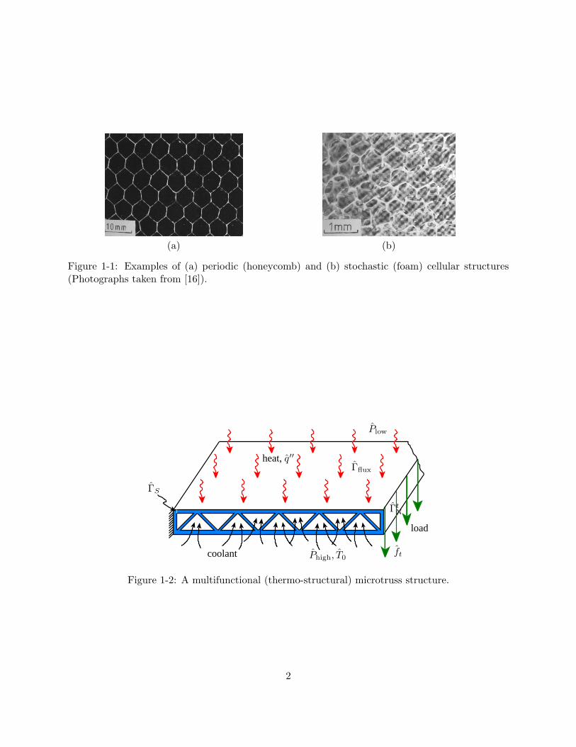
Cellular solids consist of interconnected networks of solid struts or plates which form cells [16]and may, in general, be classified as either periodic (as in lattice and prismatic materials, shownin Figure 1-1(a)) or stochastic (as in sponges and foams, shown in Figure 1-1(b)) [11]. Numerousexamples abound in nature — for instance, cork, wood, and bone — but recent materials andmanufacturing advances have allowed synthetic cellular materials to be designed and fabricated forspecific applications — for instance, lightweight structures, thermal insulation, energy absorption,and vibration control [16]. In particular, open cellular metals have received considerable attentionlargely due to their multifunctional capability: the metal struts offer relatively high structural loadcapacities at low weights, while the high thermal conductivities and open architecture allow for theefficient transfer of heat at low pumping costs.

We consider the example of a periodic open cellular structure (shown in Figure 1-2) simultane-ously designed for both heat-transfer and structural capability; this structure could represent, forinstance, a section of a combustion chamber wall in a reusable rocket engine [12, 19]. The prismaticmicrotruss consists of a frame (upper and lower faces) and a core of trusses. The structure conductsheat from a prescribed uniform flux source q′′ at the upper face to the coolant flowing through the

1

(a) (b)

Figure 1-1: Examples of (a) periodic (honeycomb) and (b) stochastic (foam) cellular structures(Photographs taken from [16]).

load

heat, q′′

coolant Phigh, T0

Plow

ft

ΓS

ΓtN

Γflux

Figure 1-2: A multifunctional (thermo-structural) microtruss structure.

2

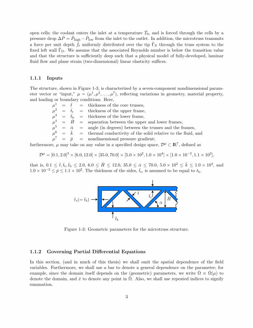
open cells; the coolant enters the inlet at a temperature T0, and is forced through the cells by apressure drop ∆P = Phigh− Plow from the inlet to the outlet. In addition, the microtruss transmitsa force per unit depth ft uniformly distributed over the tip ΓN through the truss system to thefixed left wall ΓD. We assume that the associated Reynolds number is below the transition valueand that the structure is sufficiently deep such that a physical model of fully-developed, laminarfluid flow and plane strain (two-dimensional) linear elasticity suffices.

1.1.1 Inputs

The structure, shown in Figure 1-3, is characterized by a seven-component nondimensional param-eter vector or “input,” µ = (µ1, µ2, . . . , µ7), reflecting variations in geometry, material property,and loading or boundary conditions. Here,

µ1 = t = thickness of the core trusses,µ2 = tt = thickness of the upper frame,µ3 = tb = thickness of the lower frame,µ4 = H = separation between the upper and lower frames,µ5 = α = angle (in degrees) between the trusses and the frames,µ6 = k = thermal conductivity of the solid relative to the fluid, andµ7 = p = nondimensional pressure gradient;

furthermore, µ may take on any value in a specified design space, Dµ ⊂ IR7, defined as

Dµ = [0.1, 2.0]3 × [6.0, 12.0]× [35.0, 70.0]× [5.0× 102, 1.0× 104]× [1.0× 10−2, 1.1× 102],

that is, 0.1 ≤ t, tt, tb ≤ 2.0, 6.0 ≤ H ≤ 12.0, 35.0 ≤ α ≤ 70.0, 5.0 × 102 ≤ k ≤ 1.0 × 104, and1.0× 10−2 ≤ p ≤ 1.1× 102. The thickness of the sides, ts, is assumed to be equal to tb.

tb

ttt

αHts(= tb)

Figure 1-3: Geometric parameters for the microtruss structure.

1.1.2 Governing Partial Differential Equations

In this section, (and in much of this thesis) we shall omit the spatial dependence of the fieldvariables. Furthermore, we shall use a bar to denote a general dependence on the parameter; forexample, since the domain itself depends on the (geometric) parameters, we write Ω ≡ Ω(µ) todenote the domain, and x to denote any point in Ω. Also, we shall use repeated indices to signifysummation.

3

Heat Transfer Model

The (nondimensionalized) temperature, ϑ, in the fluid satisfies the parametrized partial differentialequation

−∇2ϑ+ pVi∂ϑ

∂xi= 0, in Ωf , (1.1)

with boundary conditions

ϑ = 0, on Γinf (1.2)

∂ϑ

∂xieni = 0, on Γout

f ; (1.3)

note that the velocity field V =[0 0 V3

]T , where V3 satisfies

∇2V3 = 1 . (1.4)

Here, en denotes the unit outward normal, Ωf denotes the fluid domain, and Γinf (respectively, Γout

f )denotes the fluid inlet (respectively, outlet). The temperature in the solid is governed by

−k∇2ϑ = 0, in Ωs , (1.5)

with

k∂ϑ

∂xieni = 1 on Γflux

s , (1.6)

∂ϑ

∂xieni = 0 on Γins

s , (1.7)

reflecting the uniform flux and insulated boundary conditions, respectively. Continuity of temper-ature and heat flux along the interface Γint between the solid and fluid domains requires

ϑ∣∣s

= ϑ∣∣f

on Γint , (1.8)

−k ∂ϑ

∂xieni

∣∣∣∣s

=∂ϑ

∂xieni

∣∣∣∣f

on Γint. (1.9)

Structural (Solid Mechanics) Model

The (nondimensionalized) displacement, ui, i = 1, 2, satisfies the parametrized partial differentialequation

∂

∂xj

(Cijkl

∂uk

∂xl

)= 0, in Ωs, (1.10)

where Ωs denotes the truss domain, and the elasticity tensor Cijkl is given by

Cijkl = c1 (δikδjl + δilδjk) + c2δijδkl; (1.11)

4

here, δij is the Kronecker delta function, and c1, c2 are Lame’s constants, related to Young’smodulus, E, and Poisson’s ratio, ν, by

c1 =E

2(1 + ν), (1.12)

c2 =Eν

(1 + ν)(1− 2ν). (1.13)

The displacement and traction boundary conditions are

ui = 0 on ΓD, (1.14)σij en

j = f teti on Γt

N, (1.15)

σij enj = 0 on Γs\(ΓD ∪ Γt

N), (1.16)

where the stresses, σij are related to the displacements by

σij = Cijkl∂uk

∂xl. (1.17)

Elastic Buckling

Furthermore, it can be shown [18] that the critical load parameter λ1 ∈ IR, and associated bucklingmode ξ1 ∈ Y , are solutions to the partial differential eigenproblem

∂

∂xj

(Cijkl

∂ξk∂xl

)+ λ

∂

∂xj

(∂um

∂xlCmlkj

∂ξi∂xk

)= 0 , (1.18)

with boundary conditions

Cijkl∂ξk∂xl

enj + λ

∂ξi∂xk

fnenk = 0 on Γn

N (1.19)

Cijkl∂ξk∂xl

enj + λ

∂ξi∂xk

ftetk = 0 on Γt

N . (1.20)

(The derivation of the equivalent weak form of (1.18)-(1.20) is presented in Chapter 6.)

1.1.3 Outputs

In the engineering context — i.e., in design, optimization, control, and characterization — thequantities of interest are often not the field variables themselves, but rather functionals of thefield variables. For example, in our microtruss example the relevant “outputs” are neither thetemperature field, ϑ, the fluid velocity field, V , nor the displacement field, u; rather, we may wishto evaluate as a function of the parameter µ the average temperature along Γflux

s ,

ϑave(µ) =1

|Γfluxs |

∫Γflux

s

ϑ dΓ , (1.21)

5

the flow rate,

Q(µ) =∫

Γoutf

V3 dΓ , (1.22)

the average velocity at the outlet,

Vave =1

|Γoutf |

∫Γout

f

V3 dΓ , (1.23)

the average deflection along ΓtN,

δave(µ) = − 1|Γt

N|

∫Γt

N

u2 dΓ , (1.24)

and the normal stress near the support averaged along Γσ,

σave(µ) = − 1|Γσ|

∫Γσ

σ11(u). (1.25)

In addition, one may also be interested in eigenvalues associated with the physical system; forexample, in our microtruss example the buckling load

f±buckle(µ) = λ±1 (µ)f t , (1.26)

where λ1 is the smallest eigenvalue of (1.18)-(1.20), is also of interest. Note that evaluation of theseoutputs requires solution of the governing partial differential equations of Section 1.1.2.

1.1.4 A Design-Optimize Problem

A particular microtruss design (corresponding to a particular value of µ) has associated with it (say)operational and material costs, as well as performance merits reflecting its ability to support theapplied structural loads and efficiently transfer the applied heat to the fluid. Furthermore, a designmust meet certain constraints reflecting, for example, safety and manufacturability considerations.The goal of the design process is then to minimize costs and optimize performance while ensuringthat all design constraints are satisfied.

For example, we could define our cost function, J (µ), as a weighted sum of the area of thestructure, A(µ), (reflecting material costs), and the power, P(µ) required to pump the fluid throughthe structure (reflecting operational costs); that is,

J (µ) = aVV(µ) + aPP(µ), (1.27)

where

V(µ) = 2[(tt + tb)

(H

tanα+

t

sinα+ tb

)+H

(t

sinα+ tb

)], (1.28)

P(µ) = Q(µ), (1.29)

and aV , aP are weights which measure the relative importance of material and operational costs inthe design process.

6

Furthermore, we require that the average temperature be less than the melting temperature ofthe material:

ϑave(µ) ≤ α1ϑmax, (1.30)

the deflection be less than a prescribed limit,

δave(µ) ≤ α2δmax, (1.31)

the average normal stress near the support be less than the yield stress,

σave(µ) ≤ α3σTY , (1.32)

and the magnitude of the applied load be less than the critical buckling load, so that

1 ≤ α4λ±1 (µ) . (1.33)

We then define our feasible set, F , as the set of all values of µ ∈ Dµ which satisfy the constraints(1.30)-(1.33).

Our optimization problem can now be stated as: find the optimal design, µ∗, which satisfies

µ∗ = arg minµ∈F

J (µ); (1.34)

in other words, find that value of µ, µ∗, which minimizes the cost functional over all feasible designsµ ∈ F .

1.1.5 An Assess-Optimize Problem

The design of an engineering system, as illustrated in Section 1.1.4, involves the determination ofthe system configuration based on system requirements and environment considerations. Duringoperation, however, the state of the system may be unknown or evolving, and the system may besubjected to dynamic system requirements, as well as changing environmental conditions. The sys-tem must therefore be adaptively designed and optimized, taking into consideration the uncertaintyand variability of system state, requirements, and environmental conditions.

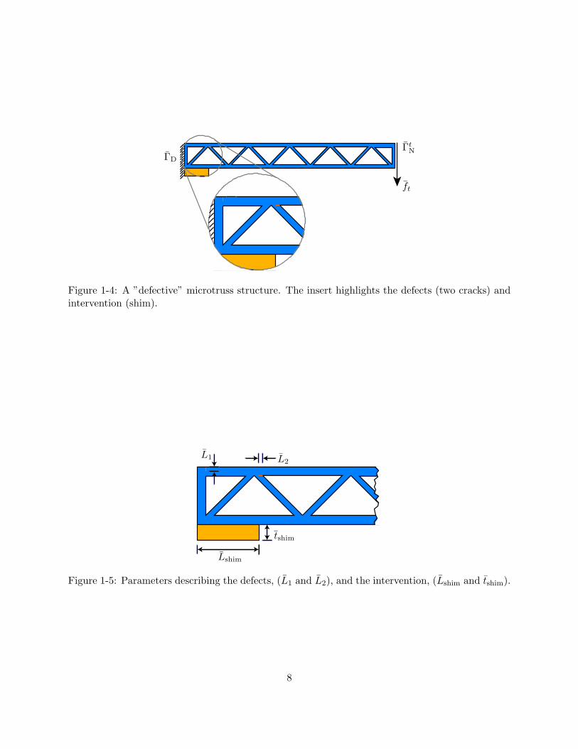
For example, we assume that extended deployment of our microtruss structure (for instance,as a component in an airplane wing) has led to the developement of defects (e.g., cracks) shown inFigure 1-4. The characteristics of the defects (e.g., crack lengths) are unknown, but we assume thatwe are privy to a set of experimental measurements which serve to assess the state of the structure.Clearly, the defects may cause the deflection to reach unacceptably high values; a shim is thereforeintroduced so as to stiffen the structure and maintain the deflection at the desired levels. However,this intervention leads to an increase in both material and operational costs. Our goal is to find,given the uncertainties in the crack lengths, the shim dimensions which minimize the weight whilehonoring our deflection constraint.

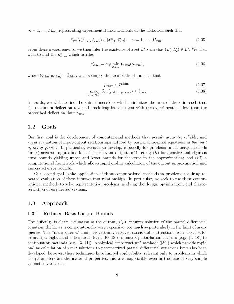
More precisely, we characterize our system with a multiparameter µ = (µcrack, µshim) whereµcrack = (L1, L2) and µshim = (Lshim, tshim). As shown in Figure 1-5, L1 and L2 are our “currentguesses” for the relative lengths of the cracks on the upper frame and truss, respectively, while tshim

and Lshim denote the thickness and length of the shim, respectively; we also denote by µ∗crack =(L∗1, L

∗2) the (real) unknown crack lengths. We further assume we are givenMexp intervals [δm

LB, δmUB],

7

ΓD

ΓtN

ft

Figure 1-4: A ”defective” microtruss structure. The insert highlights the defects (two cracks) andintervention (shim).

L1 L2

tshim

Lshim

Figure 1-5: Parameters describing the defects, (L1 and L2), and the intervention, (Lshim and tshim).

8

m = 1, . . . ,Mexp representing experimental measurements of the deflection such that

δave(µmshim, µ

∗crack) ∈ [δm

LB, δmUB], m = 1, . . . ,Mexp . (1.35)

From these measurements, we then infer the existence of a set L∗ such that (L∗1, L∗2) ∈ L∗. We then

wish to find the µ∗shim which satisfies

µ∗shim = arg minµshim

Vshim(µshim), (1.36)

where Vshim(µshim) = tshimLshim is simply the area of the shim, such that

µshim ∈ Dshim (1.37)max

µcrack∈L∗δave(µshim, µcrack) ≤ δmax . (1.38)

In words, we wish to find the shim dimensions which minimizes the area of the shim such thatthe maximum deflection (over all crack lengths consistent with the experiments) is less than theprescribed deflection limit δmax.

1.2 Goals

Our first goal is the development of computational methods that permit accurate, reliable, andrapid evaluation of input-output relationships induced by partial differential equations in the limitof many queries. In particular, we seek to develop, especially for problems in elasticity, methodsfor (i) accurate approximation of the relevant outputs of interest; (ii) inexpensive and rigorouserror bounds yielding upper and lower bounds for the error in the approximation; and (iii) acomputational framework which allows rapid on-line calculation of the output approximation andassociated error bounds.

Our second goal is the application of these computational methods to problems requiring re-peated evaluation of these input-output relationships. In particular, we seek to use these compu-tational methods to solve representative problems involving the design, optimization, and charac-terization of engineered systems.

1.3 Approach

1.3.1 Reduced-Basis Output Bounds

The difficulty is clear: evaluation of the output, s(µ), requires solution of the partial differentialequation; the latter is computationally very expensive, too much so particularly in the limit of manyqueries. The “many queries” limit has certainly received considerable attention: from “fast loads”or multiple right-hand side notions (e.g., [10, 13]) to matrix perturbation theories (e.g., [1, 48]) tocontinuation methods (e.g., [3, 41]). Analytical “substructure” methods ([30]) which provide rapidon-line calculation of exact solutions to parametrized partial differential equations have also beendeveloped; however, these techniques have limited applicability, relevant only to problems in whichthe parameters are the material properties, and are inapplicable even in the case of very simplegeometric variations.

9

Our particular approach is based on the reduced–basis method, first introduced in the late 1970sfor nonlinear structural analysis [4, 32], and subsequently developed more broadly in the 1980s and1990s [7, 8, 14, 36, 37, 42]. Our work differs from these earlier efforts in several important ways: first,we develop (in some cases, provably) global approximation spaces; second, we introduce rigorousa posteriori error estimators; and third, we exploit off-line/on-line computational decompositions(see [7] for an earlier application of this strategy within the reduced–basis context). These threeingredients allow us — for the restricted but important class of “parameter-affine” problems —to reliably decouple the generation and projection stages of reduced–basis approximation, therebyeffecting computational economies of several orders of magnitude.

We note that the operation count for the on-line stage — in which, given a new parameter value,we calculate the output of interest and associated error bound — depends only on N (typicallyvery small) and the parametric complexity of the problem; the method is thus ideally suited for therepeated and rapid evaluations required in the context of parameter estimation, design, optimiza-tion, and real-time control. Furthermore, theoretical and numerical results presented in Chapters 3(for heat conduction), 5 (for linear elasticity), and 6 (for elastic stability) show that N may indeedbe taken to be very small and that the computational economy is substantial. In addition, timingcomparisons presented in Chapter 7 for the two-dimensional microtruss example show that a singleon-line calculation of the output requires on the order of a few milliseconds, while conventionalfinite element calculation requires several seconds; the computational savings would be even largerin higher dimensions.

Furthermore, the approximate nature of reduced-basis solutions (as opposed to the exact solu-tions provided by [30]) do not pose a problem: our a posteriori error estimation procedures supplyrigorous certificates of fidelity, thus providing the necessary accuracy assessment.

1.3.2 Real-Time (Reliable) Optimization

The numerical methods proposed are rather unique relative to more standard approaches to par-tial differential equations. Reduced–basis output bound methods are intended to render partial–differential-equation solutions truly useful: essentially real–time as regards operation count; “black-box” as regards reliability; and directly relevant as regards the (limited) input–output data required.But to be truly useful, these methods must directly enable solution of “real” optimization problems— rapidly, accurately, and reliably, even in the presence of uncertainty. Our work employs thesereduced-basis output bounds in the context of “pre”-design — optimizing a system at conceptionwith respect to prescribed objectives, constraints, and environmental conditions — and adaptivedesign — optimizing a system in operation subject to evolving system characteristics, dynamicsystem requirements, and changing environmental conditions.

1.3.3 Architecture

Finally, to be truly usable, the entire methodology must reside within a special framework. Thisframework must permit the end-user to, off-line, (i) specify and define their problem in terms ofhigh-level constructs; (ii) automatically and quickly generate the online simulation and optimizationservers for their particular problem. Then, on-line, the user must be able to (i) specify the outputand input values of interest; and to receive — quasi–instantaneously — the desired prediction andcertificate of fidelity (error bound); and (ii) specify the objective, constraints, and relevant designvariables; and to receive — real-time — the desired optimal system configuration.

10

1.4 Thesis Outline

In this thesis we focus on the development of reduced-basis output bound methods for problemsin elasticity. In Chapter 2 we present an overview of reduced-basis methods, summarizing earlierwork and focusing on the (new) critical ingredients. In Chapter 3 we describe, using the heat con-duction problem for illustration, the reduced-basis approximation for coercive symmetric problemsand “compliant” outputs; we present the associated a posteriori error estimation procedures inChapter 4 . In Chapter 5 we develop the reduced-basis output bound method (approximation anda posteriori error estimation) to the linear elasticity problem and extend our methods to “noncom-pliant” outputs. In Chapter 6 we consider the nonlinear eigenvalue problem of elastic buckling; andin Chapter 7 we employ the reduced-basis methodology in the analysis, design (at conception andin operation) of our microtruss example. Finally, in Chapter 8 we conclude with some suggestionsfor future work, particularly in the area of a posteriori error estimation.

1.5 Thesis Contributions, Scope, and Limitations

In this thesis, we improve on earlier work on reduced-basis methods for linear elasticity in two ways:(i) we exploit the sparsity and symmetry of the elasticity tensor to substantially reduce both theoff-line and on-line computational cost; and (ii) we extend the methodology to allow computationof more general outputs of interest such as average stresses and buckling loads.

Furthermore, we also introduce substantial advances to the general reduced-basis methodol-ogy. First, the challenges presented by the linear elasticity operator led us to achieve a betterunderstanding of reduced-basis error estimation, and subsequently develop new techniques for con-structing rigorous (Method I) bounds for the error in the approximation. Second, we also developsimple, inexpensive (Method II) error bounds for problems in which our rigorous error estimationmethods are either inapplicable or too expensive computationally.

Finally, we apply our methods to design and optimization problems representative of appli-cations requiring repeated and rapid evaluations of the outputs of interest. We illustrate howreduced-basis methods lend themselves naturally to existing solution methods (e.g., interior pointmethods for optimization), and how they allow the development of new methods (e.g. our assess-predict-optimize methodology) which would have been intractable with conventional methods.

We note that the goals presented in Section 1.3 are by no means trivial, and the variety ofproblems (i.e., partial differential equations) that must be addressed is extensive. Indeed, this workon linear elasticity is merely a small part of a much larger effort on developing reduced-basis outputbound methods.

This thesis deals with methods that are generally applicable to linear coercive elliptic (second-order) partial differential equations with affine parameter dependence, and focuses on developingsuch methods for linear elasticity; in addition, this work also presents preliminary work on the(nonlinear) eigenvalue problem governing elastic stability, as well as some ideas for future work onthe thermoelasticity and (noncoercive) Helmholtz problem. This thesis builds on earlier work ongeneral coercive elliptic problems [43] and on linear elasticity [20].

However, reduced-basis methods have also been applied to parabolic problems [43], noncoerciveproblems [43], and problems which are (locally) non-affine in parameter [46]. These problems arenot addressed in any great detail in this thesis, save for a short summary in Chapter 2 and adiscussion of future work in Chapter 8.

11

Furthermore, in this thesis we assume that the mathematical model — particularly the parametriza-tion of the partial differential equation — is exact. A discussion reduced-basis output bounds forapproximately parametrized elliptic coercive partial differential operators may be found in [38].Some preliminary ideas based on [38] for problems with approximately parametrized data or “load-ing” (as opposed to the partial differential operator) are presented in Chapter 8.

Next, the discussion in Chapter 7 on reduced-basis methods in the context of optimizationproblems is decidedly brief; a more detailed discussion may be found in [2, 34]. A related work [17]applies reduced-basis methods to problems in optimal control.

Finally, detailed discussions of the computational architecture in which the methodology residesmay be found in [40].

12

Chapter 2

The Reduced Basis Approach: AnOverview

2.1 Introduction

As earlier indicated, our goal is the development of computational methods that permit rapid andreliable evaluation of partial-differential-equation-induced input-output relationships in the limitof many queries. In Chapter 1 we present examples of these input-output relationships, as well asproblems illustrating the “many-queries” context.

Our particular approach is based on the reduced-basis method, which recognizes that the fieldvariable is not, in fact, some arbitrary member of the infinite-dimensional solution space associatedwith the partial differential equation; rather, it resides, or evolves, on a much lower-dimensionalmanifold induced by the parametric dependence [39]. In this chapter, we provide an overview ofthe reduced-basis approach, introducing key ideas, surveying early work, highlighting more recentdevelopments, and leaving more precise definitions and detailed development to later chapters. Wefocus particularly on the critical ingredients: (i) dimension reduction, effected by global approxi-mation spaces; (ii) a posteriori error estimation, providing sharp and inexpensive upper and loweroutput bounds; and (iii) off-line/on-line computational decompositions, effecting (on-line) compu-tational economies of several orders of magnitude. These three elements allow us, for the restrictedbut important class of “parameter-affine” problems, to compute output approximations rapidly,repeatedly, with certificates of fidelity.

2.2 Abstraction

Our model problem in Chapter 1 can be stated as: for any µ ∈ Dµ ⊂ IRP , find s(µ) ∈ IR given by

s(µ) = 〈L(µ), v〉, (2.1)

where u(µ) ∈ Y is the solution of

〈A(µ)u(µ), v〉 = 〈F (µ), v〉 , ∀ v ∈ Y. (2.2)

13

Here, µ is a particular point in the parameter set, Dµ; Y is the infinite-dimensional space ofadmissible functions; A(µ) is a symmetric, continuous and coercive distributional operator, andthe loading and output functionals, F (µ) and L(µ), respectively, are bounded linear forms.1 In thelanguage of Chapter 1, (2.2) is our parametrized partial differential equation (in weak form), µ isour input parameter, u(µ) is our field variable, and s(µ) is our output.

In actual practice, Y is replaced by an appropriate “truth” finite element approximation spaceYN of dimension N defined on a suitably fine truth mesh. We then approximate u(µ) and s(µ) byuN (µ) and sN (µ), respectively, and assume that YN is sufficiently rich such that uN (µ) and sN (µ)are indistinguishable from u(µ) and s(µ).

The difficulty is clear: evaluation of the output, s(µ), requires solution of the partial differentialequation, (2.2); the latter is computationally very expensive, too much so particularly in the limitof many queries.

2.3 Dimension Reduction

In this section we give a brief overview of the essential ideas upon which the reduced basis approx-imation is based. For simplicity of exposition, we assume here and in Sections 2.4-2.5 that F andL do not depend on the parameter; in addition, we assume a “compliant” output:

〈L, v〉 ≡ 〈F, v〉 , ∀ v ∈ Y. (2.3)

2.3.1 Critical Observation

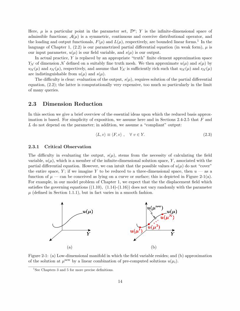
The difficulty in evaluating the output, s(µ), stems from the necessity of calculating the fieldvariable, u(µ), which is a member of the infinite-dimensional solution space, Y , associated with thepartial differential equation. However, we can intuit that the possible values of u(µ) do not “cover”the entire space, Y ; if we imagine Y to be reduced to a three-dimensional space, then u — as afunction of µ — can be conceived as lying on a curve or surface; this is depicted in Figure 2-1(a).For example, in our model problem of Chapter 1, we expect that the the displacement field whichsatisfies the governing equations ((1.10), (1.14)-(1.16)) does not vary randomly with the parameterµ (defined in Section 1.1.1), but in fact varies in a smooth fashion.

(a) (b)

Figure 2-1: (a) Low-dimensional manifold in which the field variable resides; and (b) approximationof the solution at µnew by a linear combination of pre-computed solutions u(µi).

1See Chapters 3 and 5 for more precise definitions.

14

In other words, the field variable is not some arbitrary member of the high-dimensional solu-tion space associated with the partial differential equation; rather, it resides, or “evolves,” on amuch lower–dimensional manifold induced by the parametric dependence [39]. This observation isfundamental to our approach, and is the basis for our approximation.

2.3.2 Reduced-Basis Approximation

By the preceding arguments, we see that to approximate u(µ), and hence s(µ), we need not rep-resent every possible function in Y ; instead, we need only approximate those functions in thelow-dimensional manifold “spanned” by u(µ). We could, therefore, simply calculate the solution uat several points on the manifold corresponding to different values of µ; then, for any new param-eter value, µnew, we could “interpolate between the points,” that is, approximate u(µnew) by somelinear combination of the known solutions. This notion is illustrated in Figure 2-1(b).

More precisely, we introduce a sample in parameter space,

SµN = µ1, . . . , µN (2.4)

where µn ∈ Dµ, n = 1, . . . , N. We then define our Lagrangian ([37]) reduced-basis approximationspace as

WN = spanζn ≡ u(µn), n = 1, . . . , N, (2.5)

where u(µn) ∈ Y is the solution to (2.2) for µ = µn. Our reduced-basis approximation is then: forany µ ∈ D, find

sN (µ) = 〈L, uN (µ)〉 (2.6)

where uN (µ) is the Galerkin projection of u(µ) onto WN .

〈A(µ)uN (µ), v〉 = 〈F, v〉, ∀ v ∈WN . (2.7)

In other words, we express u(µ) as a linear combination of our basis functions,

uN (µ) =N∑

j=1

uNj(µ) ζj ; (2.8)

then, choosing the basis functions as test functions (i.e., setting v = ζn, n = 1, . . . , N, in (2.7)), weobtain

AN (µ) uN (µ) = FN , (2.9)

where

(AN )i j(µ) = 〈A(µ)ζj , ζi〉 , i, j = 1, . . . , N, (2.10)(FN )i = 〈F, ζi〉 , i = 1, . . . , N. (2.11)

Our output approximation is then given by

sN (µ) = uN (µ)TLN , (2.12)

where LN = FN from (2.3).

15

2.3.3 A Priori Convergence Theory

We consider here the rate at which uN (µ) and sN (µ) converges to u(µ) and s(µ), respectively. Tobegin, it is standard to demonstrate the optimality of uN (µ) in the sense that

||u(µ)− uN (µ)||Y ≤

√γ0Aβ 0A

infwN∈WN

||u(µ)− wN ||Y . (2.13)

where || · ||Y is the norm associated with Y , and γ0A and β0

A are µ-independent constants associatedwith the operator A. Furthermore, for our compliance output, it can be shown that

s(µ)− sN (µ) = γA(µ)||u(µ)− uN (µ)||2Y , (2.14)

It follows that sN (µ) converges to s(µ) as the square of the error in uN (µ).At this point, we have not yet dealt with the question of how the sample points, µn, should

be chosen. In particular, one may ask, is there an “optimal” choice for SN? For certain simpleproblems, it can be shown [28] that, using a logarithmic point distribution, the error in the reduced-basis approximation is exponentially decreasing with N for N greater than some critical valueNcrit. More generally, numerical tests (see Chapter 3) show that the logarithmic distributionperforms considerably better than other more obvious candidates, in particular for large ranges ofthe parameter. A more detailed discussion of convergence and point distribution is presented inChapter 3.

These theoretical considerations suggest that N may, indeed, be chosen very small. However,we note from (2.11) and (2.12) that AN (µ) (and therefore uN (µ) and sN (µ)) depend on the basisfunctions, ζn, and are therefore potentially computationally very expensive. We might then ask:can we calculate sN (µ) inexpensively? We address this question in Section 2.4.

2.4 Off-Line/On-Line Computational Procedure

We recall that in this section, we assume that F and L are independent of the parameter, and thatthe output is compliant, L = F . Nevertheless, the development here can be easily extended (seeChapter 5) to the case of µ-dependent functionals L and F , and to noncompliance, L 6= F.

The output approximation, sN (µ), will be inexpensive to evaluate if we make certain assump-tions on the parametric dependence of A; these assumptions will allow us to develop off-line/on-linecomputational procedures. (See [7] for an earlier application of this strategy within the reduced-basis context.) In particular, we shall suppose that

〈A(µ)w, v〉 =QA∑q=1

Θq(µ) 〈Aqw, v〉 , (2.15)

for some finite (preferably small) integer QA. It follows that

AN (µ) =QA∑q=1

Θq(µ)AqN (µ) , (2.16)

16

whereAq

N i,j = 〈Aqζj , ζi〉, 1 ≤ i, j ≤ N, 1 ≤ q ≤ Q . (2.17)

Therefore, in the off-line stage, we compute the u(µn) and form the AqN ; this requires N (expensive)

“A” finite-element solutions, andO(QN2) finite-element-vector inner products. In the on-line stage,for any given new µ, we first form A(µ) from (2.16), then solve (2.9) for uN (µ), and finally evaluatesN (µ) = uN (µ)TLN ; this requires O(QN2) + O(2

3N3) operations and O(QN2) storage.

Thus, as required, the incremental, or marginal, cost to evaluate sN (µ) for any given new µ —as proposed in a design, optimization, or inverse-problem context — is very small: first, because(we predict) N is small, thanks to the good convergence properties of WN ; and second, because(2.9) can be very rapidly assembled and inverted, thanks to the off-line/on-line decomposition.

These off-line/on-line computational procedures clearly exploit the dimension reduction of Sec-tion 2.3. However, apart from the discussion on the a priori convergence properties of our approx-imations, we have not presented any guidelines as to what value N must be taken. Furthermore,once sN (µ) has been calculated, how does one know whether the approximation is accurate? Weaddress these issues in Section 2.5.

2.5 A Posteriori Error Estimation

From Section 2.4 we know that, in theory, we can obtain sN (µ) very inexpensively: the on–linecomputational effort scales as O(2

3N3) + O(QN2); and N can, in theory, be chosen quite small.

However, in practice, we do not know how small N can (nor how large it must) be chosen: this willdepend on the desired accuracy, the selected output(s) of interest, and the particular problem inquestion. In the face of this uncertainty, either too many or too few basis functions will be retained:the former results in computational inefficiency; the latter in unacceptable uncertainty. We thusneed a posteriori error estimators for sN (µ). Surprisingly, even though reduced–basis methodsare particularly in need of accuracy assessment — the spaces are ad hoc and pre-asymptotic,thus admitting relatively little intuition, “rules of thumb,” or standard approximation notions— a posteriori error estimation has received relatively little attention within the reduced–basisframework [32].

Efficiency and reliability of approximation are particularly important in the decision contexts inwhich reduced-basis methods typically serve. In many cases, we may wish to choose N minimallysuch that

|s(µ)− sN (µ)| ≤ εmax; (2.18)

we therefore introduce an error estimate:

∆N (µ) ≈ |s(µ)− sN (µ)| , (2.19)

which is reliable, sharp, and inexpensive to compute. Furthermore, we define the effectivity of ourerror estimate as

ηN (µ) ≡ ∆N (µ)|s(µ)− sN (µ)|

, (2.20)

and require that1 ≤ ηN (µ) ≤ ρ , (2.21)

where ρ ≈ 1. The left-hand inequality — which we denote the lower effectivity inequality —

17

guarantees that ∆N (µ) is a rigorous upper bound for the error in the output of interest, while theright-hand inequality — which we denote the upper effectivity inequality — signifies that ∆N (µ)must be a sharp bound for the true error. The former relates to reliability; while the latter leadsto efficiency. Our effectivity requirement, (2.21), then allows us to optimally select — on-line — Nsuch that

|s(µ)− sN (µ)| ≤ ∆N (µ) “=” εmax. (2.22)

In addition to the constraint on the output approximation error (2.18), we may also prescribecontstraints on the output itself; that is, we may wish to ensure that

smin ≤ s(µ) ≤ smax. (2.23)

We therefore require not only an error bound, ∆N (µ), but also lower and upper output bounds:

s−N (µ) ≤ s(µ) ≤ s+N (µ); (2.24)

we likewise require that s−N (µ) and s+N (µ) be reliable, sharp, and inexpensive to compute. We thenrequire that

smin ≤ s−N (µ) , s+N (µ) ≤ smax, (2.25)

thereby ensuring that the constraint, (2.23), is met. In many applications, satisfaction of con-straints such as (2.23) is critical to performance and, more importantly, safety; for example, theconstraints on temperature, deflection, stress, and buckling in (1.30)-(1.33) must clearly be satisfiedto ensure safe operation. Output bounds are therefore of great importance for the reduced-basisapproximations to be of any practical use.

In this work we present rigorous (or Method I) as well as asymptotic (or Method II) a posteriorierror estimation procedures; the former satisfy (2.21) and (2.24) for all N , while the latter only asN → ∞. We briefly describe these error estimators in Sections 2.5.1 and 2.5.2. A more detaileddiscussion may be found in Chapters 4 and 5.

2.5.1 Method I

Method I error estimators are based on relaxations of the error-residual equation, and are derivedfrom bound conditioners [21, 37, 47] — in essence, operator preconditioners C(µ) that satisfy (i) anadditional spectral “bound” requirement:

1 ≤ 〈A(µ)v, v〉〈C(µ)v, v〉

≤ ρ ; (2.26)

and (ii) a “computational invertibility” hypothesis:

C−1(µ) =∑

i∈I(µ)

αi(µ)C−1i (2.27)

so as to admit the reduced-basis off-line/on-line computational stratagem; here, I(µ) ⊂ 1, . . . , Iis a parameter-dependent set of indices, I is a finite (preferably small) integer, and the Ci areparameter-independent symmetric, coercive operators. In the compliance case (L = F ), the error

18

estimator is defined as∆N (µ) = 〈R(µ), C−1(µ)R(µ)〉 , (2.28)

where the residual R(µ) is defined as

〈R(µ), v〉 = 〈F, v〉 − 〈A(µ)uN (µ), v〉, (2.29)= 〈A(µ) (u(µ)− uN (µ)) , v〉, ∀ v ∈ Y , (2.30)

the output bounds are then given by

s−N (µ) = sN (µ) (2.31)s+N (µ) = sN (µ) + ∆N (µ). (2.32)

A more detailed discussion of the bounding properties of our Method I error estimators and thecorresponding off-line/on-line computational procedure, as well as “recipes” for constructing thebound conditioner C(µ), may be found in Chapter 4. The extension of the bound conditionerframework to the case of noncompliant outputs is addressed in Chapter 5. Numerical results arealso presented in Chapters 4 and 5 for simple problems in heat conduction and linear elasticity,respectively.

The essential advantage of Method I error estimators is the guarantee of rigorous bounds.However, in some cases either the associated computational expense is much too high, or there isno self-evident good choice of bound conditioners. In Section 2.5.2 we briefly describe Method IIerror estimators which eliminate these problems, albeit at the loss of absolute certainty.

2.5.2 Method II

In cases for which there are no viable rigorous error estimation procedures, we may employ simpleerror estimates which replace the true output, s(µ), in (2.19) with a finer-approximation surrogate,sM (µ). We thus set M > N and compute

∆N,M (µ) =1τ

(sM (µ)− sN (µ)) , (2.33)

for some τ ∈ (0, 1). Here sM (µ) is a reduced basis approximation to s(µ) based on a “richer”approximation space WM ⊃ WN . Since the Method II error bound is based entirely on evaluationof the output, the off-line/on-line procedure of Section 2.4 can be directly adapted; the on-lineexpense to calculate ∆N,M (µ) is therefore small. However, ∆N,M (µ) is no longer a strict upperbound for the true error: we can show [39] that ∆N,M (µ) > |s(µ) − sN (µ)| only as N → ∞. Theusefulness of Method II error estimators — in spite of their asymptotic nature — is largely due tothe rapid convergence of the reduced basis approximation.

In Chapter 4 we consider Method II error estimators in greater detail: the formulation and prop-erties of the error estimators are discussed, and numerical effectivity results for the heat conductionproblem are presented. Numerical results for the linear elasticity and elastic stability problems arealso presented in Chapters 5 and 6, respectively. Method II estimators are also used for numericaltests in the specific application (microtruss optimization) problems of Chapter 7.

19

2.6 Extensions

2.6.1 Noncompliant Outputs

In Sections 2.3-2.5 we provide a brief overview of the reduced-basis method and associated errorestimation procedure for the case of compliant outputs, L = F . In the case of more general linearbounded output functionals (L 6= F ), we introduce an adjoint or dual problem: for any µ ∈ Dµ,find ψ(µ) ∈ Y such that

〈A(µ)v, ψ(µ)〉 = −〈L, v〉 , ∀ v ∈ Y . (2.34)

We then choose a sample set in parameter space,

SµN/2 = µ1, . . . , µN/2 , (2.35)

where µi ∈ Dµ, i = 1, . . . , N (N even) and define either an “integrated” reduced-basis approxima-tion space

WN = span u(µn), ψ(µn), n = 1, . . . , N/2 (2.36)

for which the output approximation is given by

sN (µ) = 〈L, uN (µ)〉 (2.37)

where uN (µ) ∈WN is the Galerkin projection of u(µ) onto WN ,

〈A(µ)uN (µ), v〉 = 〈F, v〉 , ∀ v ∈WN ; (2.38)

or a “nonintegrated” reduced-basis approximation space

W prN = span ζpr

n = u(µn), n = 1, . . . , N/2 (2.39)

W duN = span

ζdun = ψ(µn), n = 1, . . . , N/2

(2.40)

for which the output approximation is given by

sN (µ) = 〈L(µ), uN (µ)〉 − (〈F (µ), ψN (µ)〉 − 〈A(µ)uN (µ), ψN (µ)〉) , (2.41)

where uN (µ) ∈ W prN and ψN (µ) ∈ W du

N are the Galerkin projections of u(µ) and ψ(µ) onto W prN

and W duN , respectively, i.e.,

〈A(µ)uN (µ), v〉 = 〈F (µ), v〉, ∀ v ∈W prN , (2.42)

〈A(µ)v, ψN (µ)〉 = −〈L(µ), v〉, ∀ v ∈W duN . (2.43)

As in the compliance case, the approximations uN (µ) and ψN (µ) are optimal, and the “square”effect in the convergence rate of the output is recovered. Furthermore, both the integrated andnonintegrated approaches admit an off-line/on-line decomposition similar to that described in Sec-tion 2.4 for the compliant problem; as before, the on-line complexity and storage are independent ofthe dimension of the very fine (“truth”) finite element approximation. The formulation and theoryfor noncompliant problems is discussed in greater detail in Chapter 5.

20

2.6.2 Nonsymmetric Operators

It is also possible to relax the assumption of symmetry in the operator A, permitting treatment of awider class of problems [43, 39] — a representative example is the convection-diffusion equation, inwhich the presence of the convective term renders the operator nonsymmetric. As in Section 2.3.2,we choose a sample set SN = µ1, . . . , µN, and define the reduced-basis approximation spaceWN =spanζn ≡ u(µn), n = 1, . . . , N. The reduced-basis approximation is then sN (µ) = 〈L, uN (µ)〉where uN (µ) ∈ WN satisfies 〈A(µ)uN (µ), v〉 = 〈F, v〉, ∀ v ∈ WN , and L = F . Here, uN (µ) isoptimal in the sense that

||u(µ)− uN (µ)||Y ≤(

1 +γ(µ)α(µ)

)inf

w∈WN

||u(µ)− w||Y . (2.44)

The off-line/on-line decomposition for the calculation of the output approximation is the same asfor the symmetric case, with the exception that AN and the Aq

N are no longer symmetric.The a posteriori error estimation framework may also be extended to nonsymmetric problems.

In the Method I approach, the bound conditioner C(µ) must now satisfy

1 ≤ 〈AS(µ)v, v〉〈C(µ)v, v〉

≤ ρ (2.45)

where AS(µ) = 12(A(µ)+AT (µ)) is the symmetric part of A(µ); the procedure remains the same as

for symmetric problems. In the Method II approach, since sN (µ) is no longer a strict lower boundfor s(µ), the error estimators and output bounds for noncompliant outputs (see Chapter 5) mustbe used.

2.6.3 Noncoercive Problems

There are many important problems for which the coercivity of A is lost — a representative exampleis the Helmholtz, or reduced–wave, equation. For noncoercive problems, well–posedness is nowensured only by the inf–sup condition: there exists a positive β 0

A, βA(µ), such that

0 < β 0A ≤ βA(µ) = inf

w∈Ysupv∈Y

〈A(µ)w, v〉||w||Y ||v||Y

, ∀ µ ∈ Dµ. (2.46)

Two numerical difficulties arise due to this “weaker” stability condition.The first difficulty is preservation of the inf–sup stability condition for finite dimensional ap-

proximation spaces. Although in the coercive case restriction to the space WN actually increasesstability, in the noncoercive case restriction to the space WN can easily decrease stability: the rel-evant supremizers may not be adequately represented. Loss of stability can, in turn, lead to poorapproximations — the inf–sup parameter enters in the denominator of the a priori convergenceresult. However, it is possible to resolve both of these difficulties by considering projections otherthan standard Galerkin, and “enriched” approximation spaces [26, 43]. The second numerical diffi-culty is estimation of the inf–sup parameter, important for certain classes of Method I a posteriorierror estimation techniques. In particular, βA(µ) can not typically be deduced analytically, andthus must be approximated. However, some ideas presented in Chapters 4 and 5 may be used toobtain the necessary approximation (more specifically, a lower bound) to the inf–sup parameter;this is discussed briefly in Chapter 8.

21

Method II techniques are also appropriate [39]: in particular, Method II approaches do notrequire accurate estimation of the inf-sup parameter, and thus one need be concerned only withstability in designing the reduced–basis spaces [39].

2.6.4 Eigenvalue Problems

The eigenvalues of appropriately defined partial-differential-equation eigenproblems convey criticalinformation about a physical system: in linear elasticity, the critical buckling load; in the dynamicanalysis of structures, the resonant modes; in conduction heat transfer, the equilibrium timescales.Solution of large-scale eigenvalue problems is computationally intensive: the reduced-basis methodis thus very attractive.

We first consider the extension of our approach to (weakly nonlinear) symmetric positive definiteeigenvalue problems of the form

〈A(µ)ξ(µ), v〉 = λ(µ)〈M(µ)ξ(µ), v〉 ,∀ v ∈ Y , (2.47)

where A andM are symmetric, continuous, and coercive; these assumptions on the operators implythat the eigenvalues λ are real and positive. We suppose that the output of interest is the minimumeigenvalue s(µ) = λ1(µ).

One approach [23, 39, 43] utilizes a reduced-basis predictor and “Method I” error estimatorsimilar to that for compliant symmetric problems except that (i) the reduced-basis space includeseigenfunctions associated with the first (smallest) and second eigenvalues λ1(µ) and λ2(µ), respec-tively, and (ii) the error estimator is only asymptotically valid. However, in practice, there is verylittle uncertainty in the asymptotic bounds such that the output bounds are valid even for N = 1.Furthermore, the effectivities are shown to be very good both in theory [23] and in numerical tests[39, 43].

A second approach [39] makes use of Method II error estimators, and no longer requires anestimate for the second eigenvalue. The reduced-basis space therefore includes eigenfunctions asso-ciated with only the smallest eigenvalue. The resulting bounds are asympotic, and the effectivitycan be proven [39] to be bounded from above and in fact approach a constant as N →∞.

In Chapter 6, we consider a (strongly nonlinear) eigenvalue problem (in weak form)

〈A(µ)ξ(µ), v〉 = λ(µ)〈B(µ;u(µ))ξ(µ), v〉 ,∀ v ∈ Y , (2.48)

where u(µ) satisfies〈A(µ)u(µ), v〉 = 〈F, v〉 ,∀ v ∈ Y ; (2.49)

(2.48)-(2.49) represent the equations governing the stability of elastic structures. Here, A(µ) issymmetric, continuous, and coercive, while B(µ; v) is linear in v for v ∈ Y , and is symmetric,continuous, positive semi-definite. The output of interest is the smallest eigenvalue s(µ) = λ1(µ)which corresponds to the critical buckling load; we formulate in Chapter 6 the reduced-basis ap-proximation and Method II error estimation procedures for computing the output bounds.

2.6.5 Parabolic Problems

It is also possible to treat parabolic partial differential equations of the form 〈M(µ)ut(µ), v〉 =〈A(µ)u(µ), v〉; typical examples are time-dependent problems such as unsteady heat conduction

22

— the “heat” or “diffusion” equation. The essential new ingredient is the presence of the timevariable, t.

The reduced-basis approximation and error estimator procedures are similar to those for non-compliant nonsymmetric problems, except that now the time variable is included as an additionalparameter. Thus, as in certain other time-domain model-order-reduction methods [5, 45], the basisfunctions are “snapshots” of the solution at selected time instants; however, in [43] an ensemble ofsuch series is constructed corresponding to different points in the non-time parameter domain D.For rapid convergence of the output approximation, the solutions to an adjoint problem — whichevolves backward in time — must also be included in the reduced-basis space [43].

For the temporal discretization method, many possible choices are available. The most appro-priate method — although not the only choice — is the discontinuous Galerkin method [23]. Thevariational origin of the discontinuous Galerkin approach leads naturally to rigorous output boundsfor Method I a posteriori error estimators; the Method II approach is also directly applicable. Un-der our affine assumption, off-line/on-line decompositions can be readily crafted; the complexityof the on-line stage (calculation of the output predictor and associated bound gap) is, as before,independent of the dimension of Y .

2.6.6 Locally Nonaffine Problems

An important restriction of our methods is the assumption of affine parameter dependence. Al-though many property, boundary condition, load, and even geometry variations can indeed beexpressed in the required form (2.2) for reasonably small QA, there are many problems — forexample, general boundary shape variations — which do not admit such a representation. Onesimple approach to the treatment of this more difficult class of nonaffine problems is (i) in theoff-line stage, store the ζn ≡ u(µn), and (ii) in the on-line stage, directly evaluate the reduced–basis stiffness matrix as 〈A(µ)ζj , ζi〉. Unfortunately, the operation count (respectively, storage) forthe on-line stage will now scale as O(N2 dim(Y )) (respectively, O(N dim(Y )), where dim(Y ) is thedimension of the truth (very fine) finite element approximation space: the resulting method may nolonger be competitive with advanced iterative techniques; and, in any event, “real–time” responsemay be compromised.

In [46], an approach is presented which addresses these difficulties and is slightly less generalbut potentially much more efficient. In particular, it is noted that in many cases — for example,boundary geometry modification — the nonaffine parametric dependence can be restricted to asmall subdomain of Ω, ΩII . The operator A can then be expressed as an affine/nonaffine sum,

〈A(µ)w, v〉 = 〈AI(µ)w, v〉+ 〈AII(µ)w, v〉 . (2.50)

Here AI , defined over ΩI — the majority of the domain — is affinely dependent on µ; and AII ,defined over ΩII — a small portion of the domain — is not affinely dependent on µ. It immediatelyfollows that the reduced–basis stiffness matrix can be expressed as the sum of two stiffness matricescorresponding to contributions from AI and AII respectively; that the stiffness matrix associatedwith AI admits the usual on-line/off-line decomposition described in Section 2.4; and that thestiffness matrix associated with AII requires storage (and inner product evaluation) only of ζi|ΩII

(ζi restricted to ΩII). The nonaffine contribution to the on-line computational complexity thusscales only as O(N2 dim(Y |ΩII

)), where dim(Y |ΩII) refers (in practice) to the number of finite-

element nodes located within ΩII — often extremely small. The method is therefore (almost)

23

independent of dim(Y ), though clearly the on-line code will be more complicated than in thepurely affine case.

As regards a posteriori error estimation (see [46]), the nonaffine dependence of A (even locally)precludes the precomputation and linear superposition strategy required by Method I (unless do-main decomposition concepts are exploited [22]); however, Method II directly extends to the locallynonaffine case.

24

Chapter 3

Reduced-Basis OutputApproximation:A Heat Conduction Example

3.1 Introduction

In Chapter 2 we observed that the field variable is not some arbitrary member of the infinite-dimensional solution space, but rather resides on a much lower-dimensional manifold induced by theparametric dependence; this, we noted, is the essence of the reduced-basis approximation method.In this chapter, we present a more detailed discussion of the reduced-basis output approximationmethod for linear, coercive problems, illustrated in the context of steady-state heat conduction.We focus particularly on the global approximation spaces, a priori convergence theory, and theassumption of affine parameter dependence. Numerical results for several simple problems illustratethe rapid convergence of the reduced-basis approximation to the true output, as predicted by thea priori theory. For simplicity of exposition, we consider only the compliance case in which theinhomogeneity (loading) is the same as the output functional; noncompliant outputs are addressedin Chapter 5.

We begin by stating the most general problem (and all necessary hypotheses) to which thetechniqes we develop will apply.

3.2 Abstraction

We consider a suitably regular (smooth) domain Ω ⊂ IRd, d = 1, 2, or 3, and associated functionspace Y ⊂ (H1(Ω))p, where

H1(Ω) ≡v | v ∈ L2(Ω),∇v ∈ (L2(Ω))d

, (3.1)

and

L2(Ω) ≡v |

∫Ωv2 <∞

. (3.2)

25

The inner product and norm associated with Y are given by (·, ·)Y and ||·||Y = (·, ·)1/2Y , respectively.

The corresponding dual space of Y , Y ′ is then defined as the set of all functionals F such that thedual norm of F , defined as,

||F ||Y ′ ≡ supv∈Y

〈F, v〉||v||Y

, (3.3)

is bounded; here, 〈 ·, ·〉 ≡ Y ′〈 ·, ·〉Y is the associated duality pairing. As in the previous chapters,we also define a parameter set Dµ ⊂ IRP , a particular point in which will be denoted µ. Note thatΩ is a reference domain1 and hence does not depend on the parameter.

We now introduce a distributional (second-order partial differential) operator A(µ) : Y → Y ′;we assume that A(µ) is symmetric,

〈A(µ)w, v〉 = 〈A(µ)v, w〉, ∀ w, v ∈ Y, ∀ µ ∈ Dµ, (3.4)

continuous,

〈A(µ)w, v〉 ≤ γA(µ)||w||Y ||v||Y ≤ γ0A||w||Y ||v||Y , ∀ w, v ∈ Y, ∀ µ ∈ Dµ, (3.5)

and coercive,

0 < β 0A ≤ βA(µ) = inf

w∈Y

〈A(µ)w,w〉||w||2Y

, ∀ w ∈ Y, ∀ µ ∈ Dµ. (3.6)

We also introduce the bounded linear forms F (µ) ∈ Y ′ and L(µ) ∈ Y ′, and assume that they are“compliant,”

〈L(µ), v〉 = 〈F (µ), v〉, ∀ v ∈ Y ; (3.7)

noncompliant outputs are considered in Chapter 5.We shall now make certain assumptions on the parametric dependence of A. In particular, we

shall suppose that, for some finite (preferably small) integer QA, A may be expressed as

A(µ) =QA∑q=1

Θq(µ)Aq , ∀ µ ∈ Dµ , (3.8)

where Θq : Dµ → IR and Aq : Y → Y ′. As indicated in Section 2.4, this assumption of “separability”or affine parameter dependence is crucial to computational efficiency.

We shall also suppose that, for some finite (again, preferably small) integer QF , F (µ) may beexpressed as

F (µ) =QF∑q=1

ϕqF (µ) F q , ∀ µ ∈ Dµ , (3.9)

where the ϕqF : Dµ → IR and F q ∈ Y ′. However, for simplicity of exposition we shall assume in

Sections 3.4 and 3.5 that QF = 1 and ϕ1F (µ) ≡ 1.

For simplicity of exposition, we shall (at present) assume that F — and therefore L — is inde-pendent of µ; affine dependence of the linear forms is readily admitted, however, and is addressedin Chapter 5.

1The reference domain formulation is discussed in greater detail in Section 3.4.

26

Our abstract problem statement is then: for any µ ∈ Dµ ⊂ IRP , find s(µ) ∈ IR given by

s(µ) = 〈L, u(µ)〉, (3.10)

where u(µ) ∈ Y is the solution of

〈A(µ)u(µ), v〉 = 〈F, v〉, ∀ v ∈ Y. (3.11)

In the language of Chapter 1, (3.11) is our partial differential equation (in weak form), µ is ourparameter, u(µ) is our field variable, and s(µ) is our output.

In actual practice, Y is replaced by an appropriate “truth” finite element approximation spaceYN of dimension N defined on a suitably fine truth mesh. We then approximate u(µ) and s(µ) byuN (µ) and sN (µ), respectively, and assume that YN is sufficiently rich such that uN (µ) and sN (µ)are indistinguishable from u(µ) and s(µ).

3.3 Formulation of the Heat Conduction Problem

In this section we present the strong form of the equations governing heat conduction, from whichwe derive the weak statement; we then reformulate the problem in terms of a reference (parameter-independent) domain, thus recovering the abstract formulation of Section 3.2. In this and thefollowing sections, repeated indices imply summation, and, unless otherwise indicated, indices takeon the values 1 through d, where d is the dimensionality of the problem. Furthermore, in thissection we use a bar to signify a general dependence on the parameter µ (e.g., Ω ≡ Ω(µ), or t ≡ µ)particularly when formulating the problem in a “non-reference” domain.

3.3.1 Governing Equations

We now present the governing equations and derive the weak statement for the case of a homoge-neous body; we merely state the weak statement for the more general case of an inhomogeneousbody.

Strong Form

We consider the transfer of heat in a homogeneous body Ω ⊂ IRd with boundary Γ and symmetricthermal diffusivity tensor κij . The field variable u — which here represents the temperature —satisfies the partial differential equation

∂

∂xi

(κij

∂u

∂xj

)+ b = 0 in Ω , (3.12)

with boundary conditions

u = 0 , on ΓD , (3.13)

κij∂u

∂xjeni = f , on ΓN , (3.14)

27

here, b is the rate of heat generated per unit volume, f is the prescribed heat flux input on thesurface ΓN, and en

i is the unit outward normal.

Weak Form

We now derive the weak form of the governing equations. To begin, we introduce the functionspace

Y = v ∈ (H1(Ω))p=1 | v = 0 on ΓD , (3.15)

and associated norm

||v||Y =

(∫Ω

d∑i=1

(∂v

∂xi

)2

dΩ

)1/2

. (3.16)

Multiplying (3.12) by a test function v ∈ Y and integrating over Ω, we obtain

−∫

Ωv∂

∂xi

(κij

∂u

∂xj

)dΩ =

∫Ωb v dΩ , ∀ v ∈ Y . (3.17)

Integrating by parts and applying the divergence theorem yields

−∫

Ωv∂

∂xi

(κij

∂u

∂xj

)dΩ = −

∫Γvκij

∂u

∂xjeni dΓ +

∫Ω

∂v

∂xiκij

∂u

∂xjdΩ , ∀ v ∈ Y . (3.18)

Substituting (3.18) into (3.17), and using (3.13), (3.14), and the fact that v = 0 on ΓD, we obtainas our weak statement

〈Au, v〉 = 〈F , v〉 , ∀ v ∈ Y , (3.19)

where

〈Aw, v〉 =∫

Ω

∂v

∂xiκij

∂w

∂xj(3.20)

〈F , v〉 = 〈Ff , v〉+ 〈Fb, v〉 ; (3.21)

here,

〈Ff , v〉 =∫

ΓnN

v f dΓ , 〈Fb, v〉 =∫

Ωv b dΩ . (3.22)

We now generalize (3.19)-(3.22) to the case in which Ω is inhomogeneous. Assuming that Ωconsists of R homogeneous subdomains Ωr such that

Ω =R⋃

r=1

Ωr (3.23)

28

(here, Ω denotes the closure of Ω) the weak statement takes the form of (3.19) where

〈Aw, v〉 =R∑

r=1

∫Ωr

∂v

∂xiκr

ij

∂w

∂xjdΩ (3.24)

〈F , v〉 = 〈Ff , v〉+ 〈Fb, v〉 , (3.25)

and

〈Ff , v〉 =R∑

r=1

∫Γr

N

v f r dΓ , 〈Fb, v〉 =R∑

r=1

∫Ωr

v br dΩ ; (3.26)

here, κrij is the thermal diffusivity tensor in Ωr, and Γr

N is the section of ΓN in Ωr. The derivation of

(3.24)-(3.26) is similar to that for the homogeneous case, but for the use of additional temperatureand flux continuity conditions at the interfaces between the Ωr.

3.3.2 Reduction to Abstract Form

In this section, we reformulate the problem defined by (3.24)-(3.26) so as to recover the abstractformulation of Section 3.2.

Affine Geometric Mapping

To begin, we further partition the subdomains Ωr, r = 1, . . . , R, into a total of R subdomainsΩr, r = 1, . . . , R such that there exists a reference domain Ω =

⋃Rr=1 Ωr where, for any x ∈ Ωr,

r = 1, . . . , R, its image x ∈ Ωr is given by

x = Gr(µ; x) = Gr(µ)x+ gr(µ), 1 ≤ r ≤ R ; (3.27)

we thus write∂

∂xi=∂xj

∂xi

∂

∂xj= Gji(µ)

∂

∂xj, (3.28)

andx = G(µ; x) = G(µ)x+ g(µ) , (3.29)

where x ∈ Ω, x ∈ Ω, G(µ) ∈ IRd×d is a piecewise-constant matrix, gr(µ) ∈ IRd is a piecewise-constant vector, and G(µ) : Ω → Ω is a piecewise-affine geometric mapping. We then denote theboundary of Ω as Γ, where Γ = G(µ; Γ).

Reference Domain Formulation

We now define the function space Y as Y (Ω) = Y (G−1(µ; Ω)) = Y (Ω) such that

Y = v ∈(H1(Ω)

)p=1 | v = 0 on ΓD , (3.30)

29

and for any function w ∈ Y , we define w ∈ Y such that w(x) = w(G−1(µ;x)). Furthermore, wehave

dΩ = detG−1(µ) dΩ , (3.31)dΓ =

∣∣G−1(µ) et∣∣ dΓ , (3.32)

where et is a unit vector tangent to the boundary Γ, and

∣∣G−1(µ) et∣∣ = ( d∑

i=1

(Gijet

j

)2)1/2

. (3.33)

It then follows that 〈A(µ)w, v〉 = 〈Aw, v〉 for A as in (3.24) and A(µ) given by

〈A(µ)w, v〉 =R∑

r=1

∫Ωr

(Gr

ii′(µ)∂w

∂xi

)κr

i′j′

(Gr

jj′(µ)∂v

∂xj

)det(Gr(µ))−1 dΩ , (3.34)

=R∑

r=1

∫Ωr

∂w

∂xi

(Gr

ii′(µ)κri′j′G

rjj′(µ) det(G(µ))−1

) ∂v

∂xjdΩ ∀ w, v ∈ Y , (3.35)

and 〈F (µ)w, v〉 = 〈F w, v〉 for F as in (3.25) and F (µ) given by

〈F (µ), v〉 = 〈Ff , v〉+ 〈Fb, v〉 (3.36)

where

〈Ff , v〉 =R∑

r=1

∫Γr

N

(f r∣∣∣(Gr(µ))−1 et

∣∣∣) v dΓ , 〈Fb, v〉 =R∑

r=1

∫Ωr

(br det (Gr(µ))−1

)v dΩ . (3.37)

The abstract problem statement of Section 3.2 is then recovered for

〈A(µ)w, v〉 =R∑

r=1

∫Ωr

∂w

∂xiκr

ij(µ)∂v

∂xjdΩ ∀ w, v ∈ Y , (3.38)

〈F (µ), v〉 = 〈Fb(µ), v〉+ 〈Ff (µ), v〉 (3.39)

where

〈Fb(µ), v〉 =R∑

r=1

∫Ωr

br(µ)v dΩ (3.40)

〈Ff (µ), v〉 =R∑

r=1

∫Γr

N

f r(µ)v dΓ ; (3.41)

here κrij(µ) is given by

κrij(µ) = Gr

ii′(µ) κri′j′ G

rjj′(µ) det(Gr(µ))−1 , (3.42)

30

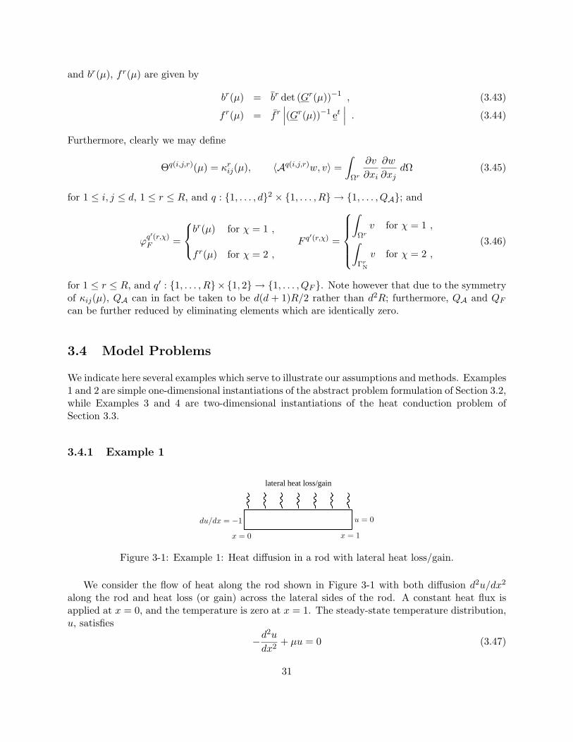
and br(µ), f r(µ) are given by

br(µ) = br det (Gr(µ))−1 , (3.43)

f r(µ) = f r∣∣∣(Gr(µ))−1 et

∣∣∣ . (3.44)

Furthermore, clearly we may define

Θq(i,j,r)(µ) = κrij(µ), 〈Aq(i,j,r)w, v〉 =

∫Ωr

∂v

∂xi

∂w

∂xjdΩ (3.45)

for 1 ≤ i, j ≤ d, 1 ≤ r ≤ R, and q : 1, . . . , d2 × 1, . . . , R → 1, . . . , QA; and

ϕq′(r,χ)F =

br(µ) for χ = 1 ,

f r(µ) for χ = 2 ,F q′(r,χ) =

∫

Ωr

v for χ = 1 ,∫Γr

N

v for χ = 2 ,(3.46)

for 1 ≤ r ≤ R, and q′ : 1, . . . , R×1, 2 → 1, . . . , QF . Note however that due to the symmetryof κij(µ), QA can in fact be taken to be d(d + 1)R/2 rather than d2R; furthermore, QA and QF

can be further reduced by eliminating elements which are identically zero.

3.4 Model Problems

We indicate here several examples which serve to illustrate our assumptions and methods. Examples1 and 2 are simple one-dimensional instantiations of the abstract problem formulation of Section 3.2,while Examples 3 and 4 are two-dimensional instantiations of the heat conduction problem ofSection 3.3.

3.4.1 Example 1

x = 1x = 0

lateral heat loss/gain

du/dx = −1 u = 0

Figure 3-1: Example 1: Heat diffusion in a rod with lateral heat loss/gain.

We consider the flow of heat along the rod shown in Figure 3-1 with both diffusion d2u/dx2

along the rod and heat loss (or gain) across the lateral sides of the rod. A constant heat flux isapplied at x = 0, and the temperature is zero at x = 1. The steady-state temperature distribution,u, satisfies

−d2u

dx2+ µu = 0 (3.47)

31

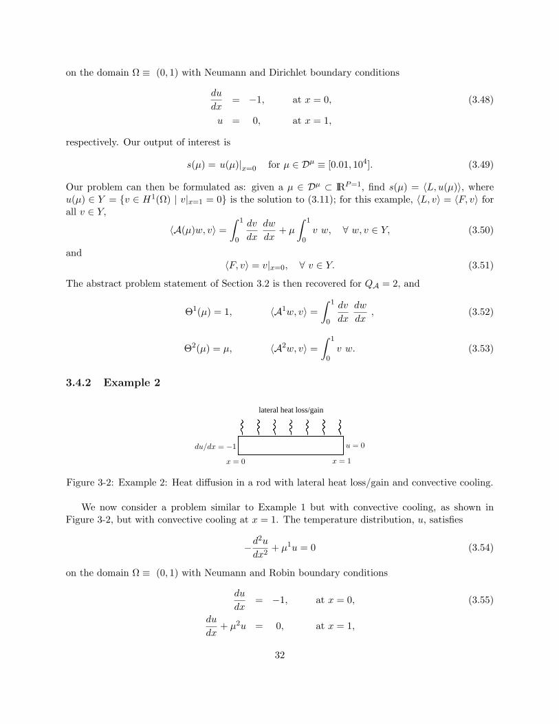
on the domain Ω ≡ (0, 1) with Neumann and Dirichlet boundary conditions

du

dx= −1, at x = 0,

u = 0, at x = 1,

(3.48)

respectively. Our output of interest is

s(µ) = u(µ)|x=0 for µ ∈ Dµ ≡ [0.01, 104]. (3.49)

Our problem can then be formulated as: given a µ ∈ Dµ ⊂ IRP=1, find s(µ) = 〈L, u(µ)〉, whereu(µ) ∈ Y = v ∈ H1(Ω) | v|x=1 = 0 is the solution to (3.11); for this example, 〈L, v〉 = 〈F, v〉 forall v ∈ Y,

〈A(µ)w, v〉 =∫ 1

0

dv

dx

dw

dx+ µ

∫ 1

0v w, ∀ w, v ∈ Y, (3.50)

and〈F, v〉 = v|x=0, ∀ v ∈ Y. (3.51)

The abstract problem statement of Section 3.2 is then recovered for QA = 2, and

Θ1(µ) = 1, 〈A1w, v〉 =∫ 1

0

dv

dx

dw

dx, (3.52)

Θ2(µ) = µ, 〈A2w, v〉 =∫ 1

0v w. (3.53)

3.4.2 Example 2

x = 1x = 0

lateral heat loss/gain

du/dx = −1 u = 0

Figure 3-2: Example 2: Heat diffusion in a rod with lateral heat loss/gain and convective cooling.

We now consider a problem similar to Example 1 but with convective cooling, as shown inFigure 3-2, but with convective cooling at x = 1. The temperature distribution, u, satisfies

−d2u

dx2+ µ1u = 0 (3.54)

on the domain Ω ≡ (0, 1) with Neumann and Robin boundary conditions

du

dx= −1, at x = 0,

du

dx+ µ2u = 0, at x = 1,

(3.55)

32

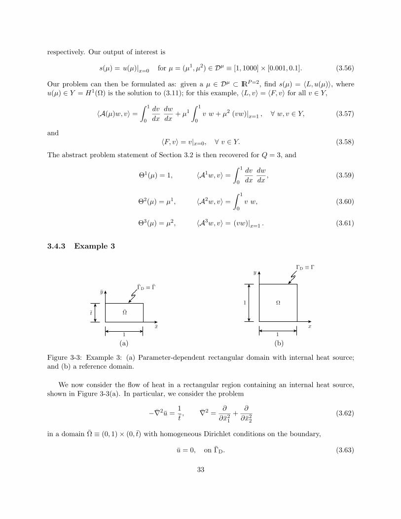
respectively. Our output of interest is

s(µ) = u(µ)|x=0 for µ = (µ1, µ2) ∈ Dµ ≡ [1, 1000]× [0.001, 0.1]. (3.56)

Our problem can then be formulated as: given a µ ∈ Dµ ⊂ IRP=2, find s(µ) = 〈L, u(µ)〉, whereu(µ) ∈ Y = H1(Ω) is the solution to (3.11); for this example, 〈L, v〉 = 〈F, v〉 for all v ∈ Y,

〈A(µ)w, v〉 =∫ 1

0

dv

dx

dw

dx+ µ1

∫ 1

0v w + µ2 (vw)|x=1 , ∀ w, v ∈ Y, (3.57)

and〈F, v〉 = v|x=0, ∀ v ∈ Y. (3.58)

The abstract problem statement of Section 3.2 is then recovered for Q = 3, and

Θ1(µ) = 1, 〈A1w, v〉 =∫ 1

0

dv

dx

dw

dx, (3.59)

Θ2(µ) = µ1, 〈A2w, v〉 =∫ 1

0v w, (3.60)

Θ3(µ) = µ2, 〈A3w, v〉 = (vw)|x=1 . (3.61)

3.4.3 Example 3

Ω

1x

ΓD ≡ Γy

t

(a)

Ω

ΓD ≡ Γy

1

1x

(b)

Figure 3-3: Example 3: (a) Parameter-dependent rectangular domain with internal heat source;and (b) a reference domain.

We now consider the flow of heat in a rectangular region containing an internal heat source,shown in Figure 3-3(a). In particular, we consider the problem

−∇2u =1t, ∇2 =

∂

∂x21

+∂

∂x22

(3.62)

in a domain Ω ≡ (0, 1)× (0, t) with homogeneous Dirichlet conditions on the boundary,

u = 0, on ΓD. (3.63)

33

Our output of interest is

s(µ) =1t

∫Ωu dΩ, for µ = t ∈ Dµ ≡ [tmin, 1.0] = [0.1, 1.0]. (3.64)

Our problem can then be formulated as: given a µ ∈ Dµ ⊂ IRP=1, find s(µ) = 〈L, u〉 whereu ∈ Y = v ∈ H1(Ω) | v|ΓD

= 0 is the solution to

〈Aw, v〉 = 〈F , v〉 , ∀ v ∈ Y ; (3.65)

here, 〈L, v〉 = 〈F , v〉 for all v ∈ Y ,

〈Aw, v〉 =∫

Ω

∂v

∂x1

∂w

∂x1+

∂v

∂x2

∂w

∂x2dΩ , ∀ w, v ∈ Y , (3.66)

and〈F , v〉 =

1t

∫Ωv dΩ , ∀ v ∈ Y . (3.67)

We now map our parameter-dependent domain Ω onto a reference domain Ω = (0, 1) × (0, 1),shown in Figure 3-3(b). The affine mapping G(x)(µ) : Ω → Ω is then given by (3.27) for R = 1,g1(µ) = 0, and

G1(µ) =

[1 0

01t

]. (3.68)

Furthermore, we have

dΩ = detG−1(µ) dΩ = t dΩ , (3.69)dΓ =

∣∣G−1(µ) et∣∣ dΓ = t dΓ . (3.70)

We may now re-formulate our problem in terms of our reference domain. Our problem is then:find s(µ) = 〈L, u(µ)〉 where u(µ) ∈ Y = v ∈ H1(Ω) | v|ΓD

= 0 is the solution to (3.11); for thisexample, 〈L, v〉 = 〈F, v〉 for all v ∈ Y,

〈A(µ)w, v〉 = t

∫Ω

∂v

∂x1

∂w

∂x1dΩ +

1t

∫Ω

∂v

∂x2

∂w

∂x2dΩ , ∀ w, v ∈ Y , (3.71)

and〈F, v〉 =

∫Ωv dΩ , ∀ v ∈ Y . (3.72)

The abstract problem statement of Section 3.2 is then recovered for P = 1, Q = 2, and

Θ1(µ) = µ, 〈A1w, v〉 =∫

Ω

∂v

∂x1

∂w

∂x1, (3.73)

Θ2(µ) =1µ, 〈A2w, v〉 =

∫Ω

∂v

∂x2

∂w

∂x2. (3.74)

34

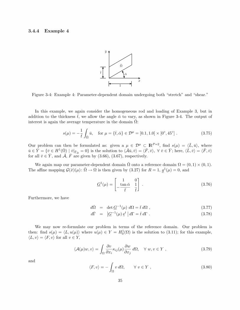
3.4.4 Example 4

y

1x

α

Ω

t

Figure 3-4: Example 4: Parameter-dependent domain undergoing both “stretch” and “shear.”

In this example, we again consider the homogeneous rod and loading of Example 3, but inaddition to the thickness t, we allow the angle α to vary, as shown in Figure 3-4. The output ofinterest is again the average temperature in the domain Ω:

s(µ) = −1t

∫Ωu, for µ = t, α ∈ Dµ = [0.1, 1.0]× [0, 45] . (3.75)

Our problem can then be formulated as: given a µ ∈ Dµ ⊂ IRP=2, find s(µ) = 〈L, u〉, whereu ∈ Y = v ∈ H1(Ω) | v|ΓD

= 0 is the solution to 〈Au, v〉 = 〈F , v〉, ∀ v ∈ Y ; here, 〈L, v〉 = 〈F , v〉for all v ∈ Y , and A, F are given by (3.66), (3.67), respectively.

We again map our parameter-dependent domain Ω onto a reference domain Ω = (0, 1)× (0, 1).The affine mapping G(x)(µ) : Ω → Ω is then given by (3.27) for R = 1, g1(µ) = 0, and

G1(µ) =

[1 0

−tan αt

1t

]. (3.76)

Furthermore, we have

dΩ = detG−1(µ) dΩ = t dΩ , (3.77)dΓ =

∣∣G−1(µ) et∣∣ dΓ = t dΓ . (3.78)

We may now re-formulate our problem in terms of the reference domain. Our problem isthen: find s(µ) = 〈L, u(µ)〉 where u(µ) ∈ Y = H1

0 (Ω) is the solution to (3.11); for this example,〈L, v〉 = 〈F, v〉 for all v ∈ Y,

〈A(µ)w, v〉 =∫

Ω

∂v

∂xiκij(µ)

∂w

∂xjdΩ, ∀ w, v ∈ Y , (3.79)

and〈F, v〉 = −

∫Ωv dΩ, ∀ v ∈ Y , (3.80)

35

and the effective diffusivity tensor κij(µ) = Gii′(µ) κi′j′ Gjj′(µ) detG−1(µ) is given by

κ =

t − tan α

− tan α1 + tan2 α

t

(3.81)

The abstract problem statement of Section 3.2 is then recovered for P = 2, QA = 3,

Θ1(µ) = t , (3.82)

Θ2(µ) =1 + tan2 α

t, (3.83)

Θ3(µ) = − tan α , (3.84)

and

〈A1w, v〉 =∫

Ω

∂v

∂x1

∂w

∂x1dΩ (3.85)

〈A2w, v〉 =∫

Ω

∂v

∂x2

∂w

∂x2dΩ , (3.86)

〈A3w, v〉 =∫

Ω

(∂v

∂x1

∂w

∂x2+

∂v

∂x2

∂w

∂x1

)dΩ . (3.87)

3.5 Reduced-Basis Output Approximation

We recall that in this chapter, we assume that A(µ) is continuous, coercive, symmetric, and affinein µ. We also assume for simplicity that L and F are independent of parameter, and L = F .

3.5.1 Approximation Space

As indicated in Chapter 2, to approximate u(µ), and hence s(µ), we need not represent everypossible function in Y ; instead, we need only approximate those functions in the low-dimensionalmanifold “spanned” by u(µ). We therefore introduce a sample in parameter space,

SµN = µ1, . . . , µN (3.88)

where µn ∈ Dµ ∈ IRP , n = 1, . . . , N. We then define our Lagrangian [37] reduced-basis approxima-tion space as

WN = spanζn ≡ u(µn), n = 1, . . . , N, (3.89)

where u(µn) ∈ Y is the solution to (2.2) for µ = µn. In actual practice, Y is replaced by anappropriate “truth” space — a finite element approximation space defined on a suitably fine truthmesh — of dimension N , where N is generally quite large.

Our reduced-basis approximation is then: for any µ ∈ Dµ, find

sN (µ) = 〈L, uN (µ)〉, (3.90)

36

where uN (µ) ∈WN is the Galerkin projection of u(µ) onto WN ,

〈A(µ)uN (µ), v〉 = 〈F, v〉, ∀ v ∈WN . (3.91)

3.5.2 A Priori Convergence Theory

Optimality

We consider here the rate at which uN (µ) and sN (µ) converges to u(µ) and s(µ), respectively. Tobegin, it is standard to demonstrate the optimality of uN (µ) in the sense that

||u(µ)− uN (µ)||Y ≤

√γA(µ)βA(µ)

infwN∈WN

||u(µ)− wN ||Y . (3.92)

To prove (3.92), we first note that since 〈Au(µ), v〉 = 〈L, v〉,∀v ∈ Y and WN ⊂ Y , it follows that

〈Au(µ), v〉 = 〈L, v〉, ∀v ∈WN . (3.93)

Subtracting (3.91) from (3.93), we obtain

〈A(u(µ)− uN (µ)), v〉 = 0, ∀ v ∈WN , (3.94)

which states that the error, u(µ)− uN (µ), is orthogonal to all members of WN . We then note thatfor any wN = uN + vN ∈WN where vN 6= 0,

〈A(µ)(u− wN ), (u− wN )〉 = 〈A(µ)((u− uN )− vN ), ((u− uN )− vN )〉 (3.95)= 〈A(µ)(u− uN ), (u− uN )〉 − 2〈A(µ)(u− uN ), vN 〉+ 〈A(µ)vN , vN 〉= 〈A(µ)(u− uN ), (u− uN )〉+ 〈A(µ)vN , vN 〉> 〈A(µ)(u− uN ), (u− uN )〉

from symmetry, Galerkin orthogonality, and coercivity; note that the µ-dependence has been omit-ted. It then follows that

〈A(µ)(u(µ)− uN (µ)), (u(µ)− uN (µ))〉 = infvN∈WN

〈A(µ)(u(µ)− vN ), (u(µ)− vN )〉 . (3.96)

Furthermore, from (3.5) we have

〈A(µ)(u(µ)− uN (µ)), (u(µ)− uN (µ))〉1/2 ≤√γA(µ) inf

vN∈WN

||u(µ)− vN ||Y ; (3.97)

and from (3.6) we have√βA(µ)||u(µ)− uN (µ)||Y ≤ 〈A(µ)(u(µ)− uN (µ)), (u(µ)− uN (µ))〉1/2 ; (3.98)

37

optimality ((3.92)) then follows from (3.97) and (3.98). Furthermore, for our compliance output,

s(µ)− sN (µ) = 〈L, u(µ)− uN (µ)〉 (3.99)= 〈A(µ)u(µ), u(µ)− uN (µ)〉 (3.100)= 〈A(µ)(u(µ)− uN (µ)), (u(µ)− uN (µ))〉 (3.101)≤ γA(µ)||u(µ)− uN (µ)||2Y , (3.102)

from (3.10), (3.11), symmetry, Galerkin orthogonality, and (3.5). Therefore, not only is uN (µ) thebest approximation among all members of WN (in the sense of (3.92)), but the output approxima-tion, sN (µ), converges to s(µ) as the square of the error in uN (µ).

Best Approximation

It now remains to bound the dependence of the error in the best approximation as a function ofN . At present, the theory [27, 28] is restricted to the case in which P = 1, Dµ = [0, µmax], and

〈A(µ)w, v〉 = 〈A0w, v〉+ µ〈A1w, v〉 (3.103)

where A0 is continuous, coercive, and symmetric, and A1 is continuous, positive semi-definite(〈A1w,w〉 ≥ 0, ∀ w ∈ Y ), and symmetric. This model problem (3.103) is rather broadly relevant,for example to variable orthotropic conductivity, variable rectilinear geometry, variable piecewise-constant conductivity, and variable Robin boundary conditions.

Following [27, 28], we suppose that the µn, n = 1, . . . , N , are logarithmically distributed in thesense that

ln(λ µn + 1

)=

n− 1N − 1

ln(λ µmax + 1

), n = 1, . . . , N, (3.104)

where λ is an upper bound for the maximum eigenvalue of A1 relative to A0. It can be shown [27]that, for N > Ncrit ≡ e ln(λ µmax + 1),

infwN∈WN

||u(µ)− wN ||Y ≤ (1 + µmax λ) ||u(0)||Y exp−(N − 1)(Ncrit − 1)

, ∀ µ ∈ Dµ . (3.105)

We observe exponential convergence, uniformly (globally) for all µ in D, with only very weak(logarithmic) dependence on the range of the parameter (µmax). (Note the constants in (3.105) arefor the particular case in which (·, ·)Y = 〈A0·, ·〉.)

The proof [27, 28] exploits a parameter–space (non-polynomial) interpolant as a surrogate forthe Galerkin approximation. As a result, the bound is not always “sharp”: we observe manycases in which the Galerkin projection is considerably better than the associated interpolant; op-timality (3.92) chooses to “illuminate” only certain points µn, automatically selecting the bestapproximation among all (combinatorially many — i.e., N !) possibilities, whereas conventional in-terpolation methods are “obligated” to use all of the points µn. We thus see why reduced–basisstate-space approximation of s(µ) via u(µ) is preferred to simple parameter-space interpolation ofs(µ) (“connecting the dots”) via (µn, s(µn)) pairs. We note, however, that the logarithmic pointdistribution (3.104) implicated by our interpolant–based arguments is not simply an artifact of theproof. We present in Figure 3-4 the maximum relative error εN (µ) over Dµ

i , i = 1, . . . , 4, for sN (µ)

38

calculated using the logarithmic distribution (3.104), a uniform distribution,

µn =n− 1N − 1

µmax 1 ≤ n ≤ N , (3.106)

and a Chebychev distribution,

µn =µmax

2

(1 + cos

(2n− 1N

π

)); (3.107)

we observe that the logarithmic distribution performs considerably better than the other moreobvious candidates.

2 4 6 8 10 12 14 16 1810

−14

10−12

10−10

10−8

10−6

10−4

10−2

100

N

ε N

LogarithmicUniformChebychev

2 4 6 8 10 12 14 16 1810

−14

10−12

10−10

10−8

10−6

10−4

10−2

100

N

ε N

LogarithmicUniformChebychev

2 4 6 8 10 12 14 16 1810

−14

10−12

10−10

10−8

10−6

10−4

10−2

100

N

ε N

LogarithmicUniformChebychev

2 4 6 8 10 12 14 16 1810

−14

10−12

10−10

10−8

10−6

10−4

10−2

100

N

ε N

LogarithmicUniformChebychev

Figure 3-5: Logarithmic vs. other distributions (grid)

The results presented in Figure 3-5 for Example 1 (P = 1) were obtained using “deterministic”grids; however, we expect that as P increases, tensor-product grids become prohibitively profligate.Fortunately, the convergence rate is not too sensitive to point selection: the theory only requires alog “on the average” distribution [27]. We present in Figure 3-6 the maximum relative error εN (µ)

39

over Dµi , i = 1, . . . , 4, for sN (µ) calculated using the logarithmic grid (3.104), a random logarithmic

distribution, and a random uniform distribution. We observe similar exponential behavior evenfor the random point distributions. We also observe that, for large ranges of the parameter, the“log-random” distribution generally performed better than the logarithmic grid; this will proveparticularly significant in higher dimensions (P > 1).

2 4 6 8 10 12 14 16 1810

−14

10−12

10−10

10−8

10−6

10−4

10−2

100

N

ε N

Logarithmic (Random)Logarithmic (Grid)

2 4 6 8 10 12 14 16 1810

−14

10−12

10−10

10−8

10−6

10−4

10−2

100

N

ε NLogarithmic (Random)Logarithmic (Grid)

2 4 6 8 10 12 14 16 1810

−14

10−12

10−10

10−8

10−6

10−4

10−2

100

N

ε N

Logarithmic (Random)Logarithmic (Grid)

2 4 6 8 10 12 14 16 1810

−14

10−12

10−10

10−8

10−6

10−4

10−2

100

N

ε N

Logarithmic (Random)Logarithmic (Grid)

Figure 3-6: Logarithmic grid vs. logarithmic random vs. other random distributions.

The result (3.105) is certainly tied to the particular form (3.103) and associated regularity ofu(µ). However, we do observe similar exponential behavior for more general operators; and, mostimportantly, the exponential convergence rate degrades only very slowly with increasing parameterdimension, P . We present in Figures 3-7, 3-8, and 3-9 the maximum relative error εN (µ) as afunction of N , at 100 randomly selected points µ in D, for Examples 2, 3, and 4, respectively. Inall three cases, the µn are chosen “log-randomly” over D: we sample from a multivariate uniformprobability density on log(µ). This is particularly important for problems in which P > 1 (such asExamples 2 and 4) since tensor-product grids are prohibitively profligate as P increases. We observethat the error is remarkably small even for very small N ; and that very rapid convergence obtainsas N →∞. We do not yet have any theory for P > 1, but certainly the Galerkin optimality plays

40

a central role, automatically selecting “appropriate” scattered-data subsets of SµN and associated

“good” weights so as to mitigate the curse of dimensionality as P increases. Furthermore, we observethat the log–random point distribution is important, as evidenced by the faster convergence (versusthe non–logarithmic uniform random point distribution) shown in Figures 3-7, 3-8, and 3-9.

0 5 10 15 20 25 30 3510

−12

10−10

10−8

10−6

10−4

10−2

100

N

ε N

Logarithmic (Random)Uniform (Random)

Figure 3-7: Convergence of the reduced-basis approximation for Example 2

0 5 10 15 20 25 30 3510

−14

10−12

10−10

10−8

10−6

10−4

10−2

100

N

ε N

Logarithmic (Random)Uniform (Random)

Figure 3-8: Convergence of the reduced-basis approximation for Example 3

3.5.3 Off-Line/On-Line Computational Procedure

The theoretical and empirical results of Sections 3.5.1 and 3.5.2 suggest that N may, indeed, bechosen very small. We now develop off-line/on-line computational procedures that exploit thisdimension reduction.

41

0 5 10 15 20 25 30 3510

−12

10−10

10−8

10−6

10−4

10−2

100

N

ε N

Logarithmic (Random)Uniform (Random)

Figure 3-9: Convergence of the reduced-basis approximation for Example 4

We first express our approximation uN (µ) to be a linear combination of the basis functions,

uN (µ) =N∑

j=1

uN j(µ) ζj (3.108)

where uN (µ) ∈ IRN ; we then choose for test functions v = ζi, i = 1, . . . , N . Inserting theserepresentations into (3.91) yields the desired algebraic equations for uN (µ) ∈ IRN ,

AN (µ) uN (µ) = FN , (3.109)

in terms of which the output can then be evaluated as

sN (µ) = uN (µ)TLN . (3.110)

Here AN (µ) ∈ IRN×N is the symmetric positive-definite (SPD) matrix with entries

AN i,j(µ) ≡ 〈A(µ)ζj , ζi〉, 1 ≤ i, j ≤ N , (3.111)

FN ∈ IRN is the “load” (and “output”) vector with entries

FN i ≡ 〈F, ζi〉, 1 ≤ i ≤ N , (3.112)

and LN = FN . We now invoke (3.8) to write

AN i,j(µ) = 〈A(µ)ζj , ζi〉 =Q∑

q=1

Θq(µ) 〈Aqζj , ζi〉 , (3.113)

42

or

AN (µ) =Q∑

q=1

Θq(µ)AqN , (3.114)

where the AqN ∈ IRN×N are given by

AqN i,j = 〈Aqζj , ζi〉 , 1 ≤ i, j ≤ N, 1 ≤ q ≤ Q . (3.115)

The off-line/on-line decomposition is now clear. In the off-line stage, we compute the u(µn) andform the Aq

N and FN : this requires N (expensive) “A” finite element solutions and O(QN2) finite-element-vector inner products. In the on-line stage, for any given new µ, we first form AN (µ)from (3.113), then solve (3.109) for uN (µ), and finally evaluate sN (µ) = uN (µ)TFN : this requiresO(QN2) +O(2

3N3) operations and O(QN2) storage.

Thus, as required, the incremental, or marginal, cost to evaluate sN (µ) for any given newµ — as proposed in a design, optimization, or inverse-problem context — is very small: first,because N is very small, typically O(10) — thanks to the good convergence properties of WN ; andsecond, because (3.109) can be very rapidly assembled and inverted — thanks to the off-line/on-linedecomposition (see [7] for an earlier application of this strategy within the reduced–basis context).For the model problems discussed in this chapter, the resulting computational savings relative tostandard (well-designed) finite-element approaches are significant.

43

44

Chapter 4

A Posteriori Error Estimation:A Heat Conduction Example

4.1 Introduction

In Chapter 3 we ascertained that sN (µ) can, in theory, be obtained very inexpensively, and that Ncan, in theory, be chosen quite small. However, in practice, we do not know how small N can (norhow large it must) be chosen: this will depend on the desired accuracy, the selected output(s) ofinterest, and the particular problem in question. In the face of this uncertainty, either too many ortoo few basis functions will be retained: the former results in computational inefficiency; the latterin unacceptable uncertainty. We thus need a posteriori error estimators for sN (µ).

In this chapter we develop methods for the a posteriori estimation of the error in reduced-basisoutput approximations. We present two general approaches for the construction of error bounds:Method I, rigorous a posteriori error estimation procedures which rely critically on the existenceof a “bound conditioner” — in essence, an operator preconditioner that (i) satisfies an additionalspectral “bound” requirement, and (ii) admits the reduced-basis off-line/on-line computationalstratagem; and Method II, a posteriori error estimation procedures which rely only on the rapidconvergence of the reduced-basis approximation, and provide simple, inexpensive error bounds,albeit at the loss of complete certainty. The general Method I approach and several “recipes” forthe construction of bound conditioners are presented in Section 4.2. The Method II is presented inSection 4.5.

As in Chapter 2, we introduce an error estimate

∆N (µ) ≈ |s(µ)− sN (µ)| , (4.1)

and define the effectivity of our error estimate as

ηN (µ) ≡ ∆N (µ)|s(µ)− sN (µ)|

; (4.2)

we recall that for reliability and efficiency, the effectivity must satisfy

1 ≤ ηN (µ) ≤ ρ , (4.3)

45

where ρ is O(1). In addition, we require lower and upper output bounds

s−N (µ) ≤ s(µ) ≤ s+N (µ), (4.4)

which are reliable, sharp, and inexpensive to compute. In this chapter, we continue to assume thatA is continuous, coercive, symmetric, and affine in µ; and that F and L are µ-independent, and〈L, v〉 = 〈F, v〉 for all v ∈ Y .

We now present the general error estimation (and output bound) procedure for both Method Iand Method II.

4.2 Method I: Uniform Error Bounds

The approach we describe here is a particular instance of a general “variational” framework for aposteriori error estimation of outputs of interest. However, the reduced-basis instantiation describedhere differs significantly from earlier applications to finite element discretization error [24, 25] anditerative solution error [35] both in the choice of (energy) relaxation and in the associated computa-tional artifice; furthermore, the “bound conditioner” formulation presented here is a generalizationof more recent work [39, 43] on a posteriori estimation for the reduced-basis method.

4.2.1 Bound Conditioner

To begin, we define the error e(µ) ∈ Y and the residual R(µ) ∈ Y ′ as

e(µ) ≡ u(µ)− uN (µ) (4.5)〈R(µ), v〉 ≡ 〈F, v〉 − 〈A(µ)uN (µ), v〉, (4.6)

from which it follows that〈A(µ)e(µ), v〉 = 〈R(µ), v〉. (4.7)

We then introduce a symmetric, continuous, and coercive bound conditioner [21, 37, 47] C(µ) : Y →Y ′ such that the minimum and maximum eigenvalues

ρmin(µ) ≡ minv∈Y

〈A(µ)v, v〉〈C(µ)v, v〉

, (4.8)

ρmax(µ) ≡ maxv∈Y

〈A(µ)v, v〉〈C(µ)v, v〉

, (4.9)

satisfy1 ≤ ρmin(µ), ρmax(µ) ≤ ρ, (4.10)

for some (preferably small) constant ρ ∈ IR.In addition to the spectral condition (4.10), we also require a “computational invertibility”

hypothesis [38, 47]. In particular, we shall require that C−1(µ) be of the form

C−1(µ) =∑

i∈I(µ)

αi(µ)C−1i (4.11)

where I(µ) ⊂ 1, . . . , I is a parameter-dependent set of indices, I is a finite (preferably small)

46

integer, and the Ci : Y → Y ′, are parameter-independent symmetric, coercive operators.

4.2.2 Error and Output Bounds

We now find e(µ) ∈ Y such that

〈C(µ)e(µ), v〉 = 〈R(µ), v〉, ∀ v ∈ Y , (4.12)

and define our lower and upper output bounds as

s−N (µ) = sN (µ) , (4.13)s+N (µ) = sN (µ) + ∆N (µ) , (4.14)

where the error estimator is given by

∆N (µ) = 〈C(µ)e(µ), e(µ)〉 (4.15)= 〈R(µ), C−1(µ)R(µ)〉 (4.16)= 〈R(µ), e(µ)〉. (4.17)

It remains to demonstrate our claim that s−N (µ) ≤ s(µ) ≤ s+N (µ) for all N ≥ 1, and to investigatethe sharpness of our bounds.

4.2.3 Bounding Properties

To begin, we first note that for any A : Y → Y ′ and any C : Y → Y ′ such that

ρmin ≤〈Av, v〉〈Cv, v〉

≤ ρmax, ∀ v ∈ Y , (4.18)

and for any U ∈ Y , W ∈ Y such that

〈AU, v〉 = 〈G, v〉, ∀ v ∈ Y , (4.19)〈CW, v〉 = 〈G, v〉, ∀ v ∈ Y , (4.20)

where G ∈ Y ′, we can show that

ρmin ≤〈CW,W 〉〈AU, U〉

≤ ρmax . (4.21)

To prove the lower inequality in (4.21) we note that 〈AU, v〉 = 〈CW, v〉 for all v ∈ Y and choosev = U to obtain

〈AU, U〉 = 〈CW,U〉≤ 〈CW,W 〉1/2〈CU, U〉1/2

≤ ρ−1/2min 〈CW,W 〉1/2〈AU, U〉1/2 (4.22)

47

from the Cauchy-Schwarz inequality and (4.18); thus ρmin〈AU,U〉 ≤ 〈CW,W 〉 as desired. To provethe upper inequality in (4.21) we choose v = W to obtain

〈CW,W 〉 = 〈AU,W 〉≤ 〈AU, U〉1/2〈AW,W 〉1/2

≤ ρ1/2max〈CW,W 〉1/2〈AU, U〉1/2 , (4.23)

from the Cauchy-Schwarz inequality and (4.18); thus 〈CW,W 〉 ≤ ρmax〈AU,U〉 as desired.We can now prove the bounding and sharpness properties of our bounds. We first prove that

s−N (µ) ≤ s(µ). We note that

s(µ)− sN (µ) = 〈A(µ) (u(µ)− uN (µ)) , u(µ)− uN (µ)〉 (4.24)≥ 0 (4.25)

from (3.95) and the coercivity of A, respectively. This lower bound proof is a standard result invariational approximation theory. We now turn to the less trivial upper bound.

To show that s+N (µ) ≥ s(µ), we note that

ηN (µ) =∆N (µ)

s(µ)− sN (µ)(4.26)

=s+N (µ)− s−N (µ)s(µ)− s−N (µ)

; (4.27)

it thus only remains to prove that ηN (µ) is greater than unity. From (4.24), and the definitions ofe(µ) and R(µ), we obtain

s(µ)− sN (µ) = 〈A(µ)e(µ), e(µ)〉 (4.28)= 〈R(µ),A−1(µ)R(µ)〉 (4.29)= 〈R(µ), e(µ)〉 , (4.30)

and thereforeηN (µ) =

〈C(µ)e(µ), e(µ)〉〈A(µ)e(µ), e(µ)〉

(4.31)

from (4.15) and (4.28). Taking A = A(µ), C = C(µ), and G = R(µ) in (4.18)-(4.21), it then followsthat

ρmin(µ) ≤ ηN (µ) ≤ ρmax(µ) , (4.32)

from (4.7), (4.8), (4.9), and (4.12). Furthermore, by construction, ρmin(µ) ≥ 1 for all µ ∈ Dµ andtherefore

ηN (µ) ≥ 1 , (4.33)

and s+N (µ) ≥ s(µ), as required. Note that the result (4.32) also indicates the sharpness of ourbounds: it follows from (4.10) that

ηN (µ) ≤ ρ . (4.34)

The result (4.32) also provides insight as to the properties of a good bound conditioner. Clearly,we wish ρmax(µ) to be as close to unity, and hence as close to ρmin(µ), as possible. We thus

48

see that good bound conditioners are similar to good (iterative) preconditioners — both satisfyρmax(µ)/ρmin(µ) ∼= 1 — except that bound conditioners must satisfy the additional spectral re-quirement ρmin(µ) ≥ 1.

4.2.4 Off-line/On-line Computational Procedure

We indicate here the off-line/on-line calculation of ∆N (µ). We recall from (4.16) that ∆N (µ) =〈R(µ), C−1(µ)R(µ)〉. From the definition of the residual (4.6), the separability assumption (3.8),and the expansion of uN (µ) in terms of the basis functions (3.108), we have

〈R(µ), v〉 = 〈F, v〉 − 〈A(µ)uN (µ), v〉

= 〈F, v〉 −QA∑q=1

N∑n=1

Θq(µ) uN n(µ) 〈Aqζn, v〉, ∀ v ∈ Y, ∀ µ ∈ Dµ . (4.35)

We now invoke the “computational invertibility” hypothesis on C(µ), (4.11), to write

∆N (µ) =∑

i∈I(µ)

αi(µ) 〈R(µ), C−1i R(µ)〉 (4.36)

=∑

i∈I(µ)

αi(µ)

⟨F −

QA∑q=1

N∑n=1

Θq(µ) uN n(µ)Aqζn,

C−1i

F − QA∑q′=1

N∑n′=1

Θq′(µ) uN n′(µ)Aq′ζn′

⟩ (4.37)

=∑

i∈I(µ)

αi(µ)

〈F, C−1i F 〉

−QA∑q=1

N∑n=1

Θq(µ) uN n(µ)(〈F, C−1

i Aqζn〉+ 〈Aqζn, C−1i F 〉

)+

QA∑q=1

QA∑q′=1

N∑n=1

N∑n′=1

Θq(µ) Θq′(µ) uN n(µ) uN n′(µ) 〈Aqζn, C−1i Aq′ζn′〉

. (4.38)

Thus, in the off-line stage, we compute the µ-independent inner products

ci = 〈F, C−1i F 〉 , (4.39)

Λiqn = −〈F, C−1

i Aqζn〉 = −〈Aqζn, C−1i F 〉 (4.40)

Γiqq′nn′ = 〈Aqζn, C−1

i Aq′ζn′〉 , (4.41)

1 ≤ i ≤ I, 1 ≤ q, q′ ≤ QA, and 1 ≤ n, n′ ≤ N ; note that (4.40) follows from the symmetry of Ci.This requires QN Aqζn multiplications, I(1+QN) C-solves, and I(Q2N2+QN+1) inner products.

49

In the on-line stage, given any new value of µ, we simply perform the sum

∆N (µ) =∑

i∈I(µ)

αi(µ)

ci + 2QA∑q=1

N∑n=1

Θq(µ) uN n(µ) Λiqn

+QA∑q=1

QA∑q′=1

N∑n=1

N∑n′=1

Θq(µ) Θq′(µ) uN n(µ) uN n′(µ) Γiqq′nn′

. (4.42)

The on-line complexity is thus, to leading order, O(|I(µ)|Q2N2) — and hence, independent of N(the dimension of Y ).

Apart from the spectral condition and invertibility requirement of Section 4.2, we have notyet specifically defined, or provided methods for developing, the bound conditioner C(µ); we shalladdress this issue in Sections 4.3 and 4.4.

4.3 Bound Conditioner Constructions — Type I

We recall from Section 4.2 that a bound conditioner is defined as a symmetric, continuous, andcoercive distributional operator C(µ) : Y → Y ′ which satisfies (i) a spectral condition —

ρmin(µ) ≡ minv∈Y

〈A(µ)v, v〉〈C(µ)v, v〉

≥ 1 , ρmax(µ) ≡ maxv∈Y

〈A(µ)v, v〉〈C(µ)v, v〉

≤ ρ , (4.43)

for some (preferably small) constant ρ ∈ IR ; and (ii) a computational invertibility condition —

C−1(µ) =∑

i∈I(µ)

αi(µ)C−1i , (4.44)

where I(µ) ⊂ 1, . . . , I is a parameter-dependent set of indices, I is a finite (preferably small)integer, and the Ci : Y → Y ′, i = 1, . . . , I, are parameter-independent symmetric, coercive operators.

In this section, we consider several classes of bound conditioners for which |I(µ)| = 1, such that(4.44) takes the simpler form

C−1(µ) = αI(µ)(µ) C−1I(µ) ; (4.45)

here, I(µ) ∈ 1, . . . , I is a parameter-dependent indicator function. In this case, the problemof constructing good bound conditioners then reduces to finding µ-independent operators Ci, i =1, . . . , I, and associated µ-dependent coefficients αi(µ) such that the spectral condition (4.43) issatisfied.

We note from (4.43) that the Ci must be “equivalent” to A in the sense that the norms || · ||Ci =〈Ci·, ·〉 and || · ||A = 〈A·, ·〉 are equivalent — there exists positive constants a and b such that [31]

a||v||Ci ≤ ||v||A ≤ b||v||Ci , ∀ v ∈ Y . (4.46)

Furthermore, if we define ρimin(µ) and ρi

max(µ) as

ρimin(µ) ≡ min

v∈Y

〈A(µ)v, v〉〈Ci v, v〉

, ρimax(µ) ≡ max

v∈Y

〈A(µ)v, v〉〈Ci v, v〉

, (4.47)

50

then for C(µ) = αi(µ)−1Ci, ρmin and ρmax are given by

ρmin(µ) = ρimin(µ)αi(µ) , ρmax(µ) = ρi

max(µ)αi(µ) (4.48)

Therefore, given any “A-equivalent,” µ-independent Ci, αi(µ)−1Ci is a bound conditioner if andonly if αi(µ)−1 is a lower bound to the minimum eigenvalue:

αi(µ)−1 ≤ ρimin(µ) , ∀ µ ∈ Dµ ; (4.49)

furthermore, since the effectivities are bounded from above and below by ρmax(µ) and ρmin(µ),respectively, αi(µ)−1 must be a sharp lower bound to ρi

min(µ), and ρimax(µ) must be as close to

ρimin(µ) as possible.

We now consider several methods for choosing the Ci and the associated αi(µ).

4.3.1 Minimum Coefficient Bound Conditioner

To begin, we recall our separability assumption on A(µ):

A(µ) =QA∑q=1

Θq(µ)Aq , ∀ µ ∈ Dµ , (4.50)

where the Θq(µ) : Dµ → IR and the Aq : Y → Y ′. We now define

A(θ) ≡QA∑q=1

θq Aq (4.51)

where θ ∈ IRQA , A(θ) : Y → Y ′, and Aq ≡ Aq. We may then write

A(Θ(µ)) = A(µ) , (4.52)

where Θ: Dµ → Dθ, and Dθ ≡ Range(Θ) ⊂ IRQA . We now assume that A(θ) is coercive for anyθ ∈ Dθ, and the Aq (and therefore the Aq) are symmetric, positive semi-definite, i.e.,

〈Aqv, v〉 ≥ 0 , ∀ v ∈ Y , 1 ≤ q ≤ QA ; (4.53)

and Dθ ⊂ IRQA+ , where IR+ refers to the positive real numbers.

Bound Conditioner

We then choose I points θi ∈ Dθ, i = 1, . . . , I, and define αi(µ), Ci, and C(µ) as

αi(µ) =(

min1≤q≤QA

(Θq(µ)θqi

))−1

, Ci =QA∑q=1

θqiA

q , (4.54)

51

and C(µ) = αI(µ)(µ)−1CI(µ), respectively, where I(µ) selects the “best” among all the points θi.The effectivity then satisfies

1 ≤ ηN (µ) ≤ max1≤m≤I

max1≤q≤QA

(Θq(µ)θqi

)min

1≤q≤QA

(Θq(µ)θqi

) , ∀ v ∈ Y ,∀ µ ∈ Dµ . (4.55)

We note that if Θ(µ) = θi, then αi(µ) = 1, 〈Civ, v〉 = 〈A(µ)v, v〉, and therefore ηN (µ) = 1. Wealso note that given any new µ ∈ Dµ, there are, in fact, I possible choices for I(µ); we can eitherestablish a definition of closeness and choose I(µ) such that θI(µ) is closest to Θ(µ); or, alternatively,consider all possible candidates and select that which yields the best effectivity.

Proof of Bounding Properties

To prove (4.55), we note that for any µ ∈ Dµ, i ∈ 1, . . . , I,

〈A(µ)v, v〉 = 〈A(Θ(µ))v, v〉 (4.56)

=

⟨QA∑q=1

Θq(µ)Aqv, v

⟩(4.57)

=

⟨QA∑q=1

(Θq(µ)θqi

)θqiA

qv, v

⟩(4.58)

≥

⟨(min

1≤q≤QA

(Θq(µ)θqi

))QA∑q=1

θqiA

q

v, v

⟩(4.59)

= 〈αi(µ)−1Civ, v〉, ∀ v ∈ Y . (4.60)

Furthermore, for any µ ∈ Dµ, i ∈ 1, . . . , I, we have

〈A(µ)v, v〉 ≤

⟨(max

1≤q≤QA

(Θq(µ)θqi

))QA∑q=1

θqiA

q

v, v

⟩, (4.61)

=max

1≤q≤QA

(Θq(µ)θqi

)min

1≤q≤QA

(Θq(µ)θqi

)〈αi(µ)−1Civ, v〉 , ∀ v ∈ Y . (4.62)

The result (4.55) directly follows from (4.59) and (4.62).

Remarks

We present in Figure 4-1, Table 4.1, and Figure 4-2 the effectivities for Examples 1-3, respectively,and θ = µ0 for different values of µ0. Note that ηN (µ) − 1 > 0 in all cases, and, as illustrated inFigures 4-1 and 4-2, ηN (µ0) = 1.

52

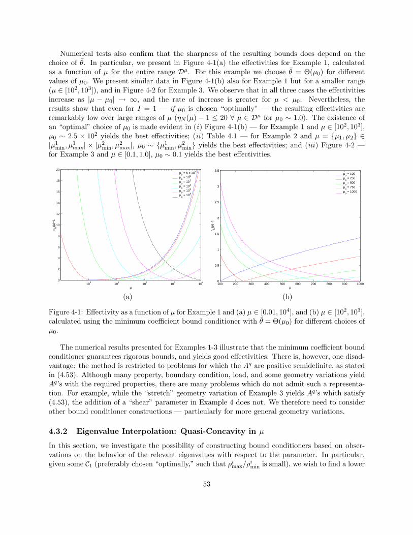
Numerical tests also confirm that the sharpness of the resulting bounds does depend on thechoice of θ. In particular, we present in Figure 4-1(a) the effectivities for Example 1, calculatedas a function of µ for the entire range Dµ. For this example we choose θ = Θ(µ0) for differentvalues of µ0. We present similar data in Figure 4-1(b) also for Example 1 but for a smaller range(µ ∈ [102, 103]), and in Figure 4-2 for Example 3. We observe that in all three cases the effectivitiesincrease as |µ − µ0| → ∞, and the rate of increase is greater for µ < µ0. Nevertheless, theresults show that even for I = 1 — if µ0 is chosen “optimally” — the resulting effectivities areremarkably low over large ranges of µ (ηN (µ) − 1 ≤ 20 ∀ µ ∈ Dµ for µ0 ∼ 1.0). The existence ofan “optimal” choice of µ0 is made evident in (i) Figure 4-1(b) — for Example 1 and µ ∈ [102, 103],µ0 ∼ 2.5 × 102 yields the best effectivities; (ii) Table 4.1 — for Example 2 and µ = µ1, µ2 ∈[µ1

min, µ1max] × [µ2

min, µ2max], µ0 ∼ µ1

min, µ2min yields the best effectivities; and (iii) Figure 4-2 —

for Example 3 and µ ∈ [0.1, 1.0], µ0 ∼ 0.1 yields the best effectivities.

100

101

102

103

104

0

2

4

6

8

10

12

14

16

18

20

µ

η N(µ

)−1

µo = 5 x 10−1

µo = 100

µo = 101

µo = 102

µo = 103

µo = 104

(a)

100 200 300 400 500 600 700 800 900 10000

0.5

1

1.5

2

2.5

3

3.5

µ

η N(µ

)−1

µo = 100

µo = 250

µo = 500

µo = 750

µo = 1000

(b)

Figure 4-1: Effectivity as a function of µ for Example 1 and (a) µ ∈ [0.01, 104], and (b) µ ∈ [102, 103],calculated using the minimum coefficient bound conditioner with θ = Θ(µ0) for different choices ofµ0.

The numerical results presented for Examples 1-3 illustrate that the minimum coefficient boundconditioner guarantees rigorous bounds, and yields good effectivities. There is, however, one disad-vantage: the method is restricted to problems for which the Aq are positive semidefinite, as statedin (4.53). Although many property, boundary condition, load, and some geometry variations yieldAq’s with the required properties, there are many problems which do not admit such a representa-tion. For example, while the “stretch” geometry variation of Example 3 yields Aq’s which satisfy(4.53), the addition of a “shear” parameter in Example 4 does not. We therefore need to considerother bound conditioner constructions — particularly for more general geometry variations.

4.3.2 Eigenvalue Interpolation: Quasi-Concavity in µ

In this section, we investigate the possibility of constructing bound conditioners based on obser-vations on the behavior of the relevant eigenvalues with respect to the parameter. In particular,given some C1 (preferably chosen “optimally,” such that ρi

max/ρimin is small), we wish to find a lower

53

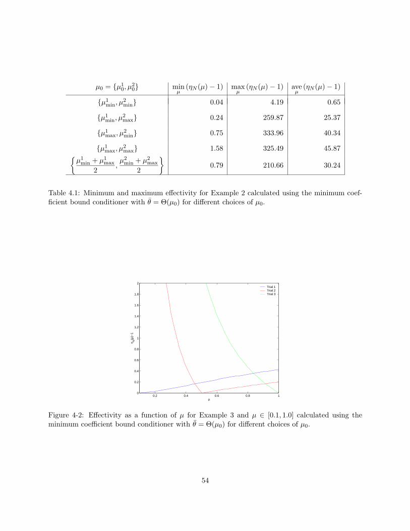
µ0 = µ10, µ

20 min

µ(ηN (µ)− 1) max

µ(ηN (µ)− 1) ave

µ(ηN (µ)− 1)

µ1min, µ

2min 0.04 4.19 0.65

µ1min, µ

2max 0.24 259.87 25.37

µ1max, µ

2min 0.75 333.96 40.34

µ1max, µ

2max 1.58 325.49 45.87

µ1min + µ1

max

2,µ2

min + µ2max

2

0.79 210.66 30.24

Table 4.1: Minimum and maximum effectivity for Example 2 calculated using the minimum coef-ficient bound conditioner with θ = Θ(µ0) for different choices of µ0.

0.2 0.4 0.6 0.8 10

0.2

0.4

0.6

0.8

1

1.2

1.4

1.6

1.8

2

µ

η N(µ

)−1

Trial 1Trial 2Trial 3

Figure 4-2: Effectivity as a function of µ for Example 3 and µ ∈ [0.1, 1.0] calculated using theminimum coefficient bound conditioner with θ = Θ(µ0) for different choices of µ0.

54

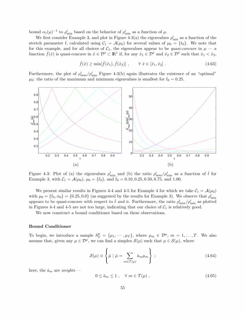
bound α1(µ)−1 to ρimin based on the behavior of ρi

min as a function of µ.We first consider Example 3, and plot in Figure 4-3(a) the eigenvalues ρi

min as a function of thestretch parameter t, calculated using C1 = A(µ0) for several values of µ0 = t0. We note thatfor this example, and for all choices of C1, the eigenvalues appear to be quasi-concave in µ — afunction f(x) is quasi-concave in x ∈ Dx ⊂ IR1 if, for any x1 ∈ Dx and x2 ∈ Dx such that x1 < x2,

f(x) ≥ min[f(x1), f(x2)] , ∀ x ∈ [x1, x2] . (4.63)

Furthermore, the plot of ρimax/ρ

imin Figure 4-3(b) again illustrates the existence of an “optimal”

µ0: the ratio of the maximum and minimum eigenvalues is smallest for t0 ∼ 0.25.

0.2 0.3 0.4 0.5 0.6 0.7 0.8 0.9

0.2

0.3

0.4

0.5

0.6

0.7

0.8

0.9

t

ρ min

i(µ

)

(a)

0.2 0.3 0.4 0.5 0.6 0.7 0.8 0.90

10

20

30

40

50

t

ρ max

i(µ

)/ρ m

ini

(µ)

(b)

Figure 4-3: Plot of (a) the eigenvalues ρimin and (b) the ratio ρi

max/ρimin as a function of t for

Example 3, with C1 = A(µ0), µ0 = t0, and t0 = 0.10, 0.25, 0.50, 0.75, and 1.00.

We present similar results in Figures 4-4 and 4-5 for Example 4 for which we take C1 = A(µ0)with µ0 = t0, α0 = 0.25, 0.0 (as suggested by the results for Example 3). We observe that ρi

min

appears to be quasi-concave with respect to t and α. Furthermore, the ratio ρimax/ρ

imin as plotted

in Figures 4-4 and 4-5 are not too large, indicating that our choice of C1 is relatively good.We now construct a bound conditioner based on these observations.

Bound Conditioner

To begin, we introduce a sample SµT = µ1, · · · , µT , where µm ∈ Dµ, m = 1, . . . , T . We also

assume that, given any µ ∈ Dµ, we can find a simplex S(µ) such that µ ∈ S(µ), where

S(µ) ≡

µ | µ =∑

m∈T (µ)

amµm

; (4.64)

here, the am are weights —0 ≤ am ≤ 1 , ∀ m ∈ T (µ) , (4.65)

55

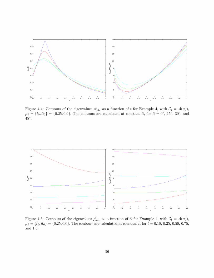
0.1 0.2 0.3 0.4 0.5 0.6 0.7 0.8 0.9 10.2

0.3

0.4

0.5

0.6

0.7

0.8

0.9

1

µ

ρ min

(µ)

0.1 0.2 0.3 0.4 0.5 0.6 0.7 0.8 0.9 10

2

4

6

8

10

12

14

16

µ

ρ max

(µ)/

ρ min

(µ)

Figure 4-4: Contours of the eigenvalues ρimin as a function of t for Example 4, with C1 = A(µ0),

µ0 = t0, α0 = 0.25, 0.0. The contours are calculated at constant α, for α = 0, 15, 30, and45.

0 5 10 15 20 25 30 35 40 450.2

0.3

0.4

0.5

0.6

0.7

0.8

0.9

1

µ

ρ min

(µ)

0 5 10 15 20 25 30 35 40 450

2

4

6

8

10

12

14

16

µ

ρ max

(µ)/

ρ min

(µ)

Figure 4-5: Contours of the eigenvalues ρimin as a function of α for Example 4, with C1 = A(µ0),

µ0 = t0, α0 = 0.25, 0.0. The contours are calculated at constant t, for t = 0.10, 0.25, 0.50, 0.75,and 1.0.

56

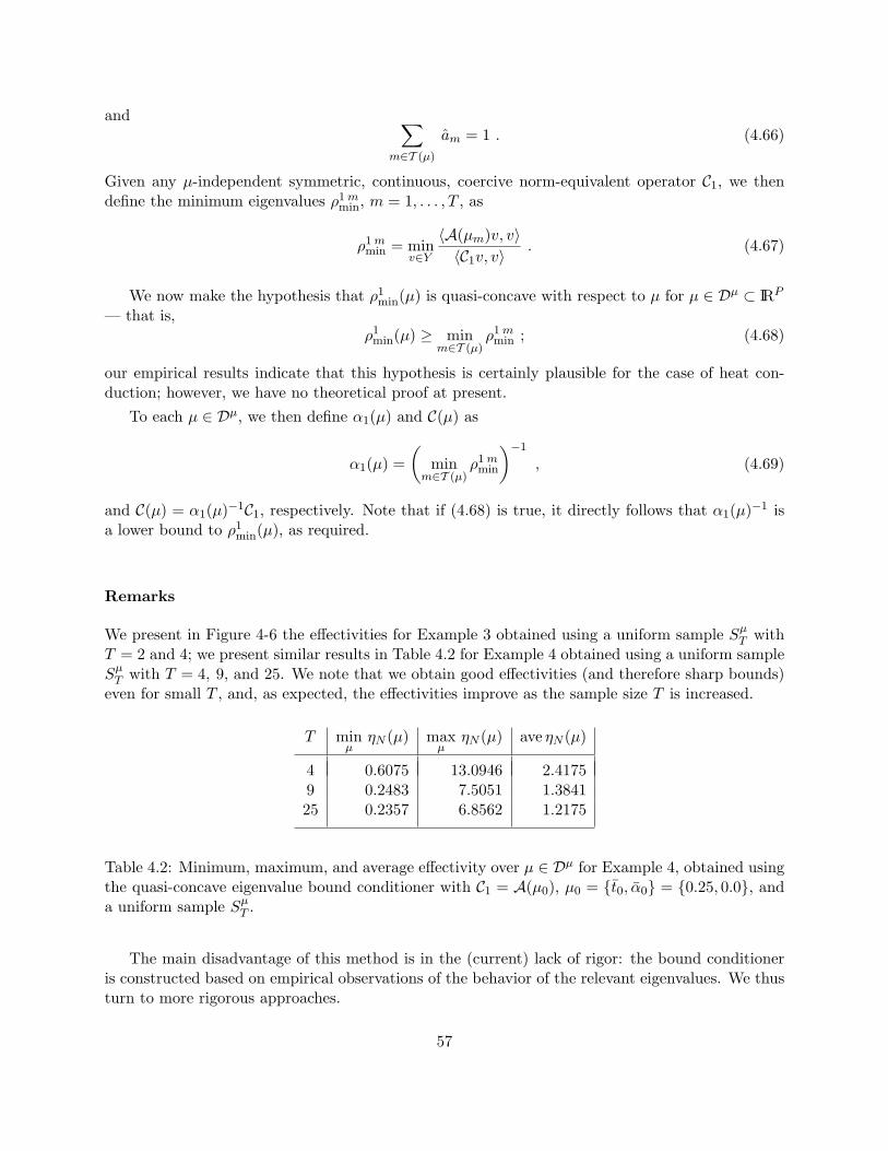
and ∑m∈T (µ)

am = 1 . (4.66)

Given any µ-independent symmetric, continuous, coercive norm-equivalent operator C1, we thendefine the minimum eigenvalues ρ1 m

min, m = 1, . . . , T , as

ρ1 mmin = min

v∈Y

〈A(µm)v, v〉〈C1v, v〉

. (4.67)

We now make the hypothesis that ρ1min(µ) is quasi-concave with respect to µ for µ ∈ Dµ ⊂ IRP

— that is,ρ1min(µ) ≥ min

m∈T (µ)ρ1 mmin ; (4.68)

our empirical results indicate that this hypothesis is certainly plausible for the case of heat con-duction; however, we have no theoretical proof at present.

To each µ ∈ Dµ, we then define α1(µ) and C(µ) as

α1(µ) =(

minm∈T (µ)

ρ1 mmin

)−1

, (4.69)

and C(µ) = α1(µ)−1C1, respectively. Note that if (4.68) is true, it directly follows that α1(µ)−1 isa lower bound to ρ1

min(µ), as required.

Remarks

We present in Figure 4-6 the effectivities for Example 3 obtained using a uniform sample SµT with

T = 2 and 4; we present similar results in Table 4.2 for Example 4 obtained using a uniform sampleSµ

T with T = 4, 9, and 25. We note that we obtain good effectivities (and therefore sharp bounds)even for small T , and, as expected, the effectivities improve as the sample size T is increased.

T minµ

ηN (µ) maxµ

ηN (µ) ave ηN (µ)

4 0.6075 13.0946 2.41759 0.2483 7.5051 1.384125 0.2357 6.8562 1.2175

Table 4.2: Minimum, maximum, and average effectivity over µ ∈ Dµ for Example 4, obtained usingthe quasi-concave eigenvalue bound conditioner with C1 = A(µ0), µ0 = t0, α0 = 0.25, 0.0, anda uniform sample Sµ

T .

The main disadvantage of this method is in the (current) lack of rigor: the bound conditioneris constructed based on empirical observations of the behavior of the relevant eigenvalues. We thusturn to more rigorous approaches.

57

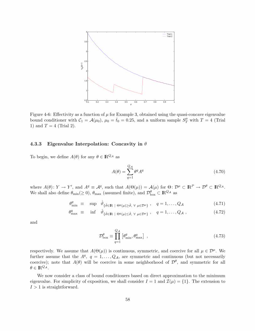
0.1 0.2 0.3 0.4 0.5 0.6 0.7 0.8 0.9 10.5

1

1.5

2

2.5

3

3.5

4

µ

η N(µ

)−1

Trial 1Trial 2

Figure 4-6: Effectivity as a function of µ for Example 3, obtained using the quasi-concave eigenvaluebound conditioner with C1 = A(µ0), µ0 = t0 = 0.25, and a uniform sample Sµ

T with T = 4 (Trial1) and T = 4 (Trial 2).

4.3.3 Eigenvalue Interpolation: Concavity in θ

To begin, we define A(θ) for any θ ∈ IRQA as

A(θ) =QA∑q=1

θqAq (4.70)

where A(θ) : Y → Y ′, and Aq ≡ Aq, such that A(Θ(µ)) = A(µ) for Θ: Dµ ⊂ IRP → Dθ ⊂ IRQA .We shall also define θmin(≥ 0), θmax (assumed finite), and Dθ

box ⊂ IRQA as

θqmin ≡ sup ϑϑ∈IR | Θq(µ)≥ϑ, ∀ µ∈Dµ , q = 1, . . . , QA (4.71)

θqmax ≡ inf ϑϑ∈IR | Θq(µ)≤ϑ, ∀ µ∈Dµ , q = 1, . . . , QA , (4.72)

and

Dθbox ≡

QA∏q=1

[θqmin, θ

qmax

], (4.73)

respectively. We assume that A(Θ(µ)) is continuous, symmetric, and coercive for all µ ∈ Dµ. Wefurther assume that the Aq, q = 1, . . . , QA, are symmetric and continuous (but not necessarilycoercive); note that A(θ) will be coercive in some neighborhood of Dθ, and symmetric for allθ ∈ IRQA .

We now consider a class of bound conditioners based on direct approximation to the minimumeigenvalue. For simplicity of exposition, we shall consider I = 1 and I(µ) = 1. The extension toI > 1 is straightforward.

58

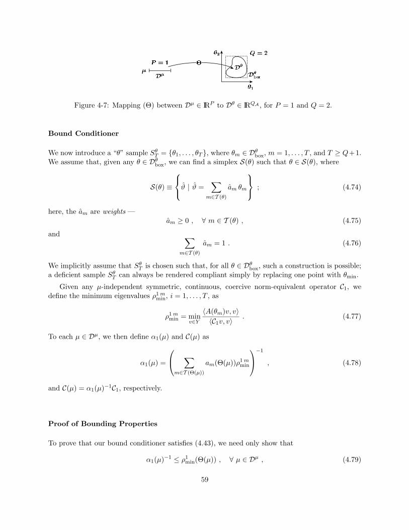
Figure 4-7: Mapping (Θ) between Dµ ∈ IRP to Dθ ∈ IRQA , for P = 1 and Q = 2.

Bound Conditioner

We now introduce a “θ” sample SθT = θ1, . . . , θT , where θm ∈ Dθ

box, m = 1, . . . , T , and T ≥ Q+1.We assume that, given any θ ∈ Dθ

box, we can find a simplex S(θ) such that θ ∈ S(θ), where

S(θ) ≡

ϑ | ϑ =∑

m∈T (θ)

am θm

; (4.74)

here, the am are weights —am ≥ 0 , ∀ m ∈ T (θ) , (4.75)

and ∑m∈T (θ)

am = 1 . (4.76)

We implicitly assume that SθT is chosen such that, for all θ ∈ Dθ

box, such a construction is possible;a deficient sample Sθ

T can always be rendered compliant simply by replacing one point with θmin.

Given any µ-independent symmetric, continuous, coercive norm-equivalent operator C1, wedefine the minimum eigenvalues ρ1 m

min, i = 1, . . . , T , as

ρ1 mmin = min

v∈Y

〈A(θm)v, v〉〈C1v, v〉

. (4.77)

To each µ ∈ Dµ, we then define α1(µ) and C(µ) as

α1(µ) =

∑m∈T (Θ(µ))

am(Θ(µ))ρ1 mmin

−1

, (4.78)

and C(µ) = α1(µ)−1C1, respectively.

Proof of Bounding Properties

To prove that our bound conditioner satisfies (4.43), we need only show that

α1(µ)−1 ≤ ρ1min(Θ(µ)) , ∀ µ ∈ Dµ , (4.79)

59

where we recall ρ1min(θ) is defined (in (4.47)) as the minimum eigenvalue

ρ1min(θ) = min

v∈Y

〈A(θ)v, v〉〈C1v, v〉

. (4.80)

To begin, we note that if a function f(θ) ∈ IR is concave in the set Dθ, then for any θ1, . . . , θT ∈Dθ,

f(a1θ1 + · · ·+ aT θT ) ≥ a1f(θ1) + · · ·+ aT f(θT ) , (4.81)

where the weights am, 1 ≤ m ≤ T satisfy (4.158) and (4.159) [6]. We now claim that the eigenvalueρ1min(θ) given by (4.80) is concave for all θ ∈ IRQA ; (4.79) then follows from the choice of the am

and the definition of α1(µ). It thus remains only to demonstrate the concavity of ρ1min(θ).

We first define Aseg(τ ; θ1, θ2) : Y → Y ′ for any two points θ1 ∈ IRQA , θ2 ∈ IRQA as

Aseg(τ ; θ1, θ2) = A(θ1 + τ(θ2 − θ1)) (4.82)

=QA∑q=1

θq1A

q + τ

QA∑q=1

(θq2 − θq

1)Aq , (4.83)

≡ Aseg0 (θ1, θ2) + τAseg

1 (θ1, θ2) , (4.84)

for τ ∈ [0, 1]. We then define ρseg(τ ; θ1, θ2) as the eigenvalue and ξseg(τ ; θ1, θ2) as the correspondingeigenvector of

〈Aseg(τ ; θ1, θ2)ξseg(τ ; θ1, θ2), v〉 = λseg(τ ; θ1, θ2)〈C1 ξseg(τ ; θ1, θ2), v〉 , ∀ v ∈ Y , (4.85)

such that the eigenvectors are normalized with respect to C1:

〈C1ξseg(τ ; θ1, θ2), ξseg(τ ; θ1, θ2)〉 = 1 . (4.86)

Defining ρsegmin to be the minimum eigenvalue of (4.85), we can then write

ρsegmin(τ ; θ1, θ2) = ρ1

min(θ1 + τ(θ2 − θ1)) . (4.87)

We would therefore like to show that for any θ1 ∈ IRQA , θ2 ∈ IRQA ,

d2

dτ2ρsegmin(τ ; θ1, θ2) ≤ 0 , ∀ τ ∈ [0, 1] , (4.88)

from which it follows that ρsegmin(θ) is concave for all θ ∈ IRQA .

For brevity, we shall henceforth omit the dependence on (θ1, θ2).

We first differentiate the normalization (4.86) with respect to τ to obtain⟨C1

d

dτξseg(τ), ξseg(τ)

⟩= 0 , (4.89)

60

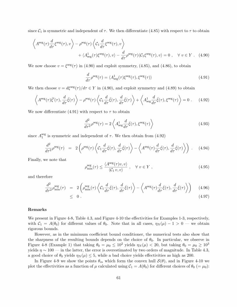
since C1 is symmetric and independent of τ . We then differentiate (4.85) with respect to τ to obtain⟨Aseg(τ)

d

dτξseg(τ), v

⟩− ρseg(τ)

⟨C1

d

dτξseg(τ), v

⟩+ 〈A1

seg(τ)ξseg(τ), v〉 − d

dτρseg(τ)〈C1ξ

seg(τ), v〉 = 0 , ∀ v ∈ Y . (4.90)

We now choose v = ξseg(τ) in (4.90) and exploit symmetry, (4.85), and (4.86), to obtain

d

dτρseg(τ) = 〈A1

seg(τ)ξseg(τ), ξseg(τ)〉 (4.91)

We then choose v = dξseg(τ)/dτ ∈ Y in (4.90), and exploit symmetry and (4.89) to obtain⟨Aseg(τ)ξ′(τ),

d

dτξ(τ)

⟩− ρseg(τ)

⟨C1

d

dτξ(τ),

d

dτξ(τ)

⟩+⟨A1

seg

d

dτξ(τ), ξseg(τ)

⟩= 0 . (4.92)

We now differentiate (4.91) with respect to τ to obtain

d2

dτ2ρseg(τ) = 2

⟨A1

seg

d

dτξ(τ), ξseg(τ)

⟩(4.93)

since Aseg1 is symmetric and independent of τ . We then obtain from (4.92)

d2

dτ2ρseg(τ) = 2

(ρseg(τ)

⟨C1

d

dτξ(τ),

d

dτξ(τ)

⟩−⟨Aseg(τ)

d

dτξ(τ),

d

dτξ(τ)

⟩). (4.94)

Finally, we note that

ρsegmin(τ) ≤

〈Aseg(τ)v, v〉〈C1 v, v〉

, ∀ v ∈ Y , (4.95)

and therefore

d2

dτ2ρsegmin(τ) = 2

(ρsegmin(τ)

⟨C1

d

dτξ(τ),

d

dτξ(τ)

⟩−⟨Aseg(τ)

d

dτξ(τ),

d

dτξ(τ)

⟩)(4.96)

≤ 0 . (4.97)

Remarks

We present in Figure 4-8, Table 4.3, and Figure 4-10 the effectivities for Examples 1-3, respectively,with C1 = A(θ0) for different values of θ0. Note that in all cases, ηN (µ) − 1 > 0 — we obtainrigorous bounds.

However, as in the minimum coefficient bound conditioner, the numerical tests also show thatthe sharpness of the resulting bounds depends on the choice of θ0. In particular, we observe inFigure 4-8 (Example 1) that taking θ0 = µ0 ≤ 102 yields ηN (µ) < 20, but taking θ0 = µ0 ≥ 103

yields η ∼ 100 — in the latter, the error is overestimated by two orders of magnitude. In Table 4.3,a good choice of θ0 yields ηN (µ) ≤ 5, while a bad choice yields effectivities as high as 200.

In Figure 4-9 we show the points θm which form the convex hull S(θ), and in Figure 4-10 weplot the effectivities as a function of µ calculated using C1 = A(θ0) for different choices of θ0 (= µ0):

61

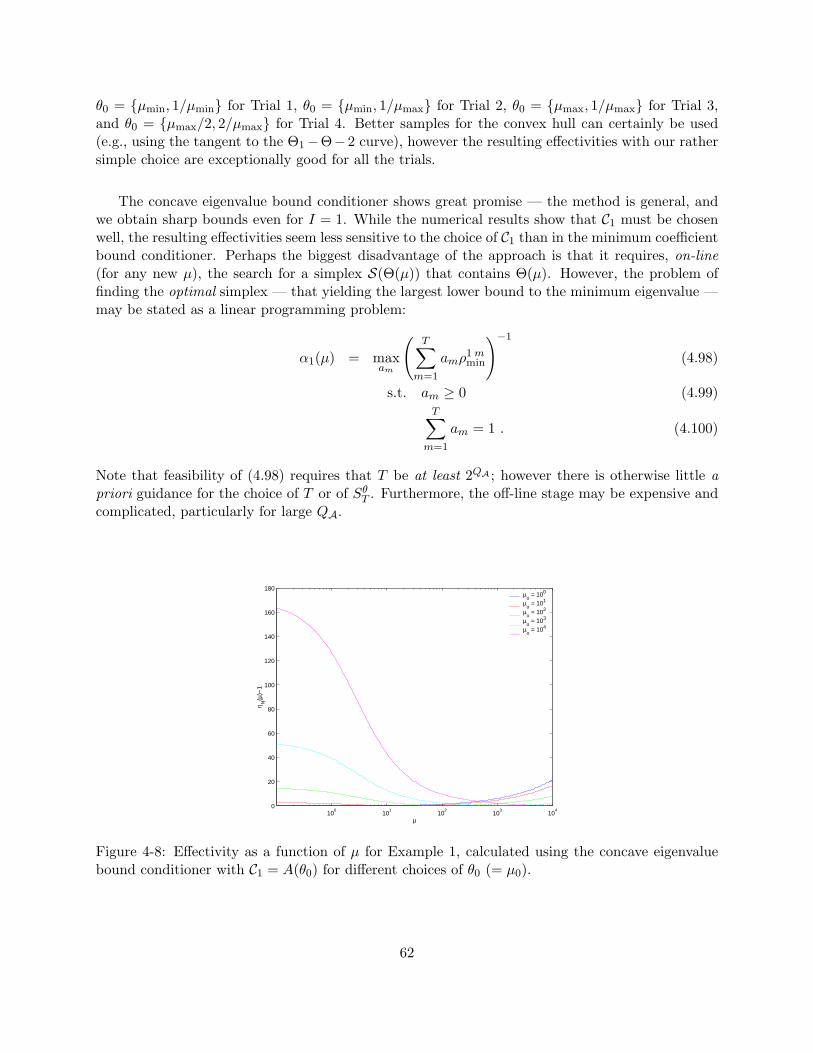
θ0 = µmin, 1/µmin for Trial 1, θ0 = µmin, 1/µmax for Trial 2, θ0 = µmax, 1/µmax for Trial 3,and θ0 = µmax/2, 2/µmax for Trial 4. Better samples for the convex hull can certainly be used(e.g., using the tangent to the Θ1−Θ− 2 curve), however the resulting effectivities with our rathersimple choice are exceptionally good for all the trials.

The concave eigenvalue bound conditioner shows great promise — the method is general, andwe obtain sharp bounds even for I = 1. While the numerical results show that C1 must be chosenwell, the resulting effectivities seem less sensitive to the choice of C1 than in the minimum coefficientbound conditioner. Perhaps the biggest disadvantage of the approach is that it requires, on-line(for any new µ), the search for a simplex S(Θ(µ)) that contains Θ(µ). However, the problem offinding the optimal simplex — that yielding the largest lower bound to the minimum eigenvalue —may be stated as a linear programming problem:

α1(µ) = maxam

(T∑

m=1

amρ1 mmin

)−1

(4.98)

s.t. am ≥ 0 (4.99)T∑

m=1

am = 1 . (4.100)

Note that feasibility of (4.98) requires that T be at least 2QA ; however there is otherwise little apriori guidance for the choice of T or of Sθ

T . Furthermore, the off-line stage may be expensive andcomplicated, particularly for large QA.

100

101

102

103

104

0

20

40

60

80

100

120

140

160

180

µ

η N(µ

)−1

µo = 100

µo = 101

µo = 102

µo = 103

µo = 104

Figure 4-8: Effectivity as a function of µ for Example 1, calculated using the concave eigenvaluebound conditioner with C1 = A(θ0) for different choices of θ0 (= µ0).

62

θ0 ≡= µ10, µ

20 min

µ(ηN (µ)− 1) max

µ(ηN (µ)− 1) ave

µ(ηN (µ)− 1)

µ1min, µ

2min 0.0379 4.1912 0.6447

µ1min, µ

2max 0.7467 236.6623 34.4212

µ1max, µ

2min 0.7859 230.7950 33.7431

µ1max, µ

2max 0.0279 3.8670 0.5852

µ1min + µ1

max

2,µ2

min + µ2max

2

0.9724 149.2957 22.3509

Table 4.3: Minimum, maximum, and average effectivity for Example 2, calculated using the concaveeigenvalue bound conditioner with T = 16, a uniform sample Sθ

T , and C1 = A(θ0) for differentchoices of θ0.

0 0.2 0.4 0.6 0.8 10

1

2

3

4

5

6

7

8

9

10

11

Θ1(µ)

Θ2(µ

)

Θ1(µ)−Θ

2(µ) curve

SθT

Figure 4-9: Sample SθT and the convex hull, S(θ)

for all θ ∈ Dθ.

0.1 0.2 0.3 0.4 0.5 0.6 0.7 0.8 0.9 10

2

4

6

8

10

12

14

16

18

µ

η N(µ

)−1

Trial 1Trial 2Trial 3Trial 4

Figure 4-10: Effectivity as a function of µ for Ex-ample 3, calculated using the concave eigenvaluebound conditioner with C1 = A(θ0) for differentchoices of θ0.

63

4.3.4 Effective Property Bound Conditioners

We now consider a problem which, after affine mapping, is described by

〈A(µ)w, v〉 =R∑

r=1

∫Ωr

∂w

∂xiκr

ij(µ)∂v

∂xj=

R∑r=1

∫Ωr

D[w ]κr(µ)D[ v ] (4.101)

where Ω = ∪Rr=1Ω

r is the domain (Ωi∩Ωj = 0, and Ω denotes the closure of Ω), κr(µ) ∈ IRd×d, d =1, 2, or 3, is the symmetric, positive definite effective diffusivity tensor (e.g., due to geometricmapping or non-isotropic properties), and

Di[w ] =∂w

∂xi, 1 ≤ i ≤ d . (4.102)

We now present a class of bound conditioners based on approximations to the diffusivity tensor.For simplicity of exposition, we shall again consider I = 1 and I(µ) = 1. The extension to I > 1is straightforward.

Bound Conditioner

We assume that we can find a set of µ-independent, symmetric, positive-definite matrices κr,r = 1, . . . , R, such that such that

vTκr(µ) vvT κr v

> 0 , ∀ v ∈ IR2 ,∀ µ ∈ Dµ , 1 ≤ r ≤ R . (4.103)

We then choose α1(µ), C1, and C(µ) such that

1 ≤ α1(µ)vTκr(µ) vvT κr v

≤ ρ , ∀ v ∈ IR2 ,∀ µ ∈ Dµ , 1 ≤ r ≤ R , (4.104)

〈C1w, v〉 =R∑

r=1

∫Ωr

DT [w ]κrD[ v ] , (4.105)

and C(µ) = α1(µ)−1C1. It then follows that

1 ≤ ηN (µ) ≤ ρ . (4.106)

Proof of Bounding Properties

We note that, by construction,

DT [ v ]κr(µ)D[ v ] ≥ α1(µ)−1DT [ v ] κr D[ v ] , ∀ v ∈ Y ,∀ µ ∈ Dµ , 1 ≤ r ≤ R ; (4.107)

64

it therefore follows that

〈A(µ)v, v〉〈C(µ)v, v〉

=

R∑r=1

∫Ωr

DT [ v ]κr(µ)D[ v ]

R∑r=1

∫Ωr

α1(µ)−1DT [ v ] κr D[ v ]

(4.108)

≥ 1 , ∀ v ∈ Y . (4.109)

Furthermore, sinceDT [ v ]κr(µ)D[ v ] ≤ ρ

(α1(µ)−1DT [ v ] κr D[ v ]

), (4.110)

it follows from (4.108) that

〈A(µ)v, v〉〈C(µ)v, v〉

≤

R∑r=1

ρα1(µ)−1

∫Ωr

DT [ v ]κrDT [ v ]

R∑r=1

α1(µ)−1

∫Ωr

DT [ v ]κrD[ v ]

(4.111)

≤ ρ . (4.112)

The result (4.106) directly follows from (4.108) and (4.112).

Finding the κr and associated α1(µ) that satisfy (4.104) and minimize ρ is not so trivial, but itis not difficult to find suboptimal solutions. We shall illustrate this with two general examples.

We first consider the case R = 1 and

κ1(µ) =[a(µ) 0

0 b(µ)

](4.113)

with amax ≥ a(µ) ≥ amin ≥ 0, and bmax ≥ b(µ) ≥ bmin ≥ 0; these conditions ensure that the κ1(µ)is symmetric, positive-definite. We then define α1(µ) = 1, and choose

κ1 =[amin 0

0 bmin

]. (4.114)

Clearly, our choices satisfy (4.104) since

minv∈IR2

α1(µ)vTκ1(µ)vvT κ1v

= min[a(µ)amin

,b(µ)bmin

](4.115)

≥ 1 , (4.116)

and

maxv∈IR2

α1(µ)vTκ1(µ)vvT κ1v

= max[a(µ)amin

,b(µ)bmin

](4.117)

≤ maxµ∈Dµ

(max

[a(µ)amin

,b(µ)bmin

]). (4.118)

65

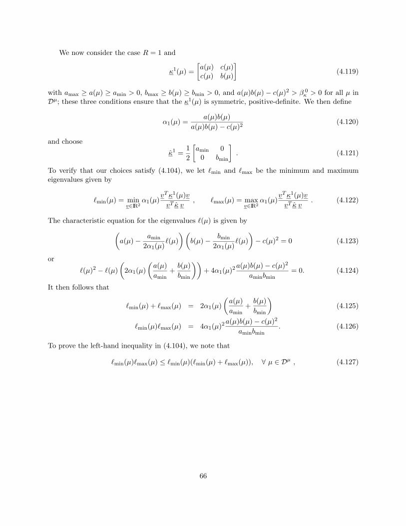
We now consider the case R = 1 and

κ1(µ) =[a(µ) c(µ)c(µ) b(µ)

](4.119)

with amax ≥ a(µ) ≥ amin > 0, bmax ≥ b(µ) ≥ bmin > 0, and a(µ)b(µ)− c(µ)2 > β 0κ > 0 for all µ in

Dµ; these three conditions ensure that the κ1(µ) is symmetric, positive-definite. We then define

α1(µ) =a(µ)b(µ)

a(µ)b(µ)− c(µ)2(4.120)

and choose

κ1 =12

[amin 0

0 bmin

]. (4.121)

To verify that our choices satisfy (4.104), we let `min and `max be the minimum and maximumeigenvalues given by

`min(µ) = minv∈IR2

α1(µ)vTκ1(µ)vvT κ v

, `max(µ) = maxv∈IR2

α1(µ)vTκ1(µ)vvT κ v

. (4.122)

The characteristic equation for the eigenvalues `(µ) is given by(a(µ)− amin

2α1(µ)`(µ)

)(b(µ)− bmin

2α1(µ)`(µ)

)− c(µ)2 = 0 (4.123)

or

`(µ)2 − `(µ)(

2α1(µ)(a(µ)amin

+b(µ)bmin

))+ 4α1(µ)2

a(µ)b(µ)− c(µ)2

aminbmin= 0. (4.124)

It then follows that

`min(µ) + `max(µ) = 2α1(µ)(a(µ)amin

+b(µ)bmin

)(4.125)

`min(µ)`max(µ) = 4α1(µ)2a(µ)b(µ)− c(µ)2

aminbmin. (4.126)

To prove the left-hand inequality in (4.104), we note that

`min(µ)`max(µ) ≤ `min(µ)(`min(µ) + `max(µ)), ∀ µ ∈ Dµ , (4.127)

66

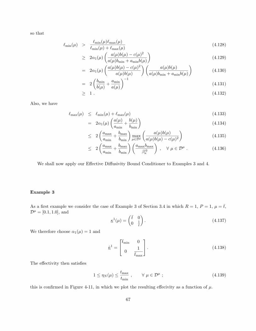
so that

`min(µ) >`min(µ)`max(µ)`min(µ) + `max(µ)

(4.128)

≥ 2α1(µ)(

a(µ)b(µ)− c(µ)2

a(µ)bmin + aminb(µ)

)(4.129)

= 2α1(µ)(a(µ)b(µ)− c(µ)2

a(µ)b(µ)

)(a(µ)b(µ)

a(µ)bmin + aminb(µ)

)(4.130)

= 2(bmin

b(µ)+amin

a(µ)

)−1

(4.131)

≥ 1 . (4.132)

Also, we have

`max(µ) ≤ `min(µ) + `max(µ) (4.133)

= 2α1(µ)(a(µ)amin

+b(µ)bmin

)(4.134)

≤ 2(amax

amin+bmax

bmin

)maxµ∈Dµ

(a(µ)b(µ)

a(µ)b(µ)− c(µ)2

)(4.135)

≤ 2(amax

amin+bmax

bmin

)(amaxbmax

β 0κ

), ∀ µ ∈ Dµ . (4.136)

We shall now apply our Effective Diffusivity Bound Conditioner to Examples 3 and 4.

Example 3

As a first example we consider the case of Example 3 of Section 3.4 in which R = 1, P = 1, µ = t,Dµ = [0.1, 1.0], and

κ1(µ) =(t 00 1

t

). (4.137)

We therefore choose α1(µ) = 1 and

κ1 =

tmin 0

01

tmax

. (4.138)

The effectivity then satisfies

1 ≤ ηN (µ) ≤ tmax

tmin, ∀ µ ∈ Dµ ; (4.139)

this is confirmed in Figure 4-11, in which we plot the resulting effecivity as a function of µ.

67

0.1 0.2 0.3 0.4 0.5 0.6 0.7 0.8 0.9 10

0.5

1

1.5

2

2.5

3

µ

η N(µ

)−1

Figure 4-11: Effectivity as a function of µ forExample 3 obtained using the effective propertybound conditioner.

0.1 0.2 0.3 0.4 0.5 0.6 0.7 0.8 0.9 10

5

10

15

20

25

30

35

40

µ

η N(µ

)−1

α = 0.0α = 15.0α = 30.0α = 45.0

Figure 4-12: Effectivity as a function of µ forExample 4 obtained using the effective propertybound conditioner.

Example 4

As a second example, we consider Example 4 of Section 3.4 in which R = 1, P = 2, µ = (t, α),Dµ = [0.1, 1.0]× [0, 45], and

κ1(µ) =

t − tan α

− tan α1 + tan2 α

t

(4.140)

We therefore chooseα1(µ) = 1 + tan2 α (4.141)

and

κ1 =12

tmin 0

01

tmax

(4.142)

The effectivity then satisfies

1 ≤ ηN (µ) ≤ 4tmax

tmin, ∀ µ ∈ Dµ ; (4.143)

this is also confirmed in Figure 4-12, in which we plot the resulting effecivity as a function of µ.

Remarks

The effective property bound conditioner presents several advantages: numerical tests show thatthe effective property conditioner yields good effectivities and, unlike the concave eigenvalue boundconditioner, the computational cost is independent of QA. Furthermore, although the method isrestricted to problems of the form (4.101), unlike the minimum coefficient conditioner it is applicable

68

even for general geometry variations. However, in Chapter 5 we shall see that the requirement thatκ be positive-definite proves very restrictive — the relevant material property tensor is no longerpositive-definite.

4.4 Bound Conditioner Constructions — Type II

We recall from Section 4.2 our “computational invertibility” assumption:

C−1(µ) =∑

i∈I(µ)

αi(µ)C−1i (4.144)

where I(µ) ⊂ 1, . . . , I is a parameter-dependent set of indices, I is a finite (preferably small)integer, and the Ci : Y → Y ′, are parameter-independent symmetric, coercive operators.

We now consider a particular class of bound conditioners in which C−1(µ) is constructed as adirect approximation to A−1(µ).

4.4.1 Convex Inverse Bound Conditioner

To begin, we recall our separability assumption (3.8) on A(µ), and assume that A(µ) takes theparticular (slightly different) form

A(µ) = A0 +QA∑q=1

Θq(µ)Aq , ∀ µ ∈ Dµ , (4.145)

where the Θq(µ) : Dµ → IR+,0, q = 1, . . . , QA; here, IR+,0 refers to the non-negative real numbers.We also assume that A0 : Y → Y ′ is symmetric, continuous, and coercive, and that the Aq : Y → Y ′,q = 1, . . . , QA are symmetric, continuous, and positive-semidefinite, i.e.,

〈A0w,w〉 > 0 , ∀ w ∈ Y , (4.146)〈Aqw,w〉 ≥ 0 , ∀ w ∈ Y , 1 ≤ q ≤ QA ; (4.147)

it follows that A(µ) is symmetric, continuous, and coercive for all µ ∈ Dµ.

For any θ ∈ IRQA+,0, we now define A(θ) : Y → Y ′ as

A(θ) = A0 +QA∑q=1

θq Aq , (4.148)

where Aq ≡ Aq, 0 ≤ q ≤ QA. We may then write

A(Θ(µ)) = A(µ) , (4.149)

where Θ: Dµ ⊂ IRP → Dθ ⊂ IRQA , and Dθ is the range of Θ. We shall also define θmin(≥ 0), θmax

69

(assumed finite), and Dθbox ⊂ IRQA

+,0 as

θqmin ≡ sup ϑϑ∈IR+ | Θq(µ)≥ϑ, ∀ µ∈Dµ , q = 1, . . . , QA (4.150)

θqmax ≡ inf ϑϑ∈IR+ | Θq(µ)≤ϑ, ∀ µ∈Dµ , q = 1, . . . , QA , (4.151)

and

Dθbox ≡

QA∏q=1

[θqmin, θ

qmax

], (4.152)

respectively. It follows that A(θ) is symmetric, continuous, and coercive for all θ ∈ Dθbox.

Finally, we note that our compliance output can be expressed as an energy:

s(µ) = 〈L, u(µ)〉 (4.153)= 〈F, u(µ)〉 (4.154)= 〈A(Θ(µ))u(µ), u(µ)〉 , (4.155)

or, equivalently,s(µ) = 〈F,A−1(Θ(µ))F 〉 , (4.156)

where A−1(θ) is the (symmetric, coercive) inverse of A(θ).

Bound Conditioner Formulation

We now introduce a “θ” sample SθT = θ1, . . . , θT , where θi ∈ Dθ

box, i = 1, . . . , T . We assume that,given any θ ∈ Dθ

box, we can find a simplex S(θ) such that θ ∈ S(θ), where

S(θ) ≡

ϑ | ϑ =∑

i∈T (θ)

ai θi

; (4.157)

here, T (θ) ⊂ 1, . . . , T is an index set of cardinality QA, and the ai are weights —

0 ≤ ai ≤ 1 , ∀ r ∈ T (θ) , (4.158)

and ∑i∈T (θ)

ai = 1 . (4.159)

In words, the simplex S(θ) is a polyhedral set, defined by |T (θ)| vertices T (θ) chosen such that S(θ)contains θ. We implicitly assume that Sθ

T is chosen such that, for all θ ∈ Dθbox, such a construction

is possible; a deficient sample SθT can always be rendered compliant simply by replacing one point

with θmin.To each µ in Dµ we then associate (i) a point θ(µ) ∈ Dθ

box, such that

θq(µ) ≤ Θq(µ) , 1 ≤ q ≤ QA , (4.160)

70

(ii) an index set I(µ) given byI(µ) = T (θ(µ)) , (4.161)

and (iii) a set of weights ai(θ(µ)), such that

θ(µ) =∑

i∈I(µ)

ai(θ(µ)) θi . (4.162)

We then choose the αi(µ) and Cm as

αi(µ) = ai(θ(µ)) (4.163)Ci = A−1(θi) (4.164)

so that C(µ) is given by

C(µ) =∑

i∈I(µ)

αi(µ)C−1i =

∑i∈I(µ)

αi(µ)A−1(θi)

−1

. (4.165)

(Clearly, C−1(µ) (and therefore C(µ)) is symmetric positive-definite.) In words, C−1(µ) is an ap-proximation to A−1(Θ(µ)) constructed as a convex combination of A−1 at “neighboring” θ.

Proof of Bounding Properties

To prove that the bound conditioner (4.163) provides uniform bounds, we shall need to demonstratecertain properties of the quadratic form associated with A−1(θ). To begin, we define J : Dθ

box×Y ′ →IR as

J (θ, G) = 〈G, A−1(θ) G〉 , (4.166)

Also, given θ1 ∈ Dθbox, θ2 ∈ Dθ

box, and τ ∈ [0, 1], we define

J seg(τ ; θ1, θ2; G) = J (θ1 + τ(θ2 − θ1), G) (4.167)

We also define Aseg(τ ; θ1, θ2) = A(θ1 + τ(θ2 − θ1)). We can then write

Aseg(τ ; θ1, θ2) = A1 +QA∑q=1

θq1 A

q + τ

QA∑q=1

(θq2 − θq

1)Aq . (4.168)

andJ seg(τ ; θ1, θ2; G) = 〈G, (Aseg(τ ; θ1, θ2))−1 G〉 . (4.169)

We now consider the monotonicity and convexity of J (θ) in the parameter θ; in particular, wecan prove [47] that:

(A) J (θ, G) is a non-increasing function: for any θ1 ∈ Dθbox, θ2 ∈ Dθ

box, such that θ2 ≥ θ1 (i.e.,θq2 ≥ θq

1, q = 1, . . . , QA),J (θ2, G) ≤ J (θ1, G) , ∀ G ∈ Y ′ ; (4.170)

71

(B) J (θ, G) is a convex function of θ: for any θ1 ∈ Dθbox, θ2 ∈ Dθ

box, and for all τ ∈ [0, 1],

J (θ1 + τ(θ2 − θ1), G) ≤ (1− τ) J (θ1, G) + τ J (θ2, G) , ∀ G ∈ Y ′ . (4.171)

We shall refer to (4.170) and (4.171) as Propositions (A) and (B), respectively.Assuming that Propositions (A) and (B) are indeed true (we shall present the proofs subse-

quently), we can prove that our bound conditioner satisfies the spectral condition. We recall fromSection 4.2 that the effectivity may be written as

ηN (µ) =〈R(µ), C−1(µ)R(µ)〉〈R(µ),A−1(µ)R(µ)〉

. (4.172)

From the definitions (4.163) and (4.145) we immediately note that

ηN (µ) =

∑i∈I(µ)

αi(µ) J (θi,R(µ))

J (Θ(µ),R(µ)). (4.173)

But from the construction of the αj(µ), the choice of I(µ), Proposition (B), classical results inconvex analysis, and Proposition (A), it directly follows that, for any G ∈ Y ′ (and therefore forG = R(µ)), ∑

i∈I(µ)

αi(µ) J (θi, G) ≥ J (θ(µ), G) ≥ J (Θ(µ), G) , (4.174)

which concludes the proof. It now remains only to prove Propositions (A) and (B).

Proof of Proposition (A)

To prove Proposition (A), we need only demonstrate that, for any (fixed) θ1, θ2 such that θ2 ≥ θ1,and any (fixed) G ∈ Y ′,

d

dτJ seg(τ ; θ1, θ2; G) ≤ 0, ∀ τ ∈ [0, 1] . (4.175)

To evaluate dJ seg/dτ , we note that

d

dτJ seg(τ ; θ1, θ2; G) =

⟨G,

d

dτ

((Aseg)−1(τ ; θ1, θ2)

), G

⟩; (4.176)

it thus remains only to show that d(Aseg(τ ; θ1, θ2))−1/dτ is symmetric negative-semidefinite.To this end, we note that (Aseg(τ ; θ1, θ2))−1 Aseg(τ ; θ1, θ2) = II (the identity), and thus

d

dτ(Aseg(τ ; θ1, θ2))

−1Aseg(τ ; θ1, θ2) + (Aseg(τ ; θ1, θ2))−1 d

dτ(Aseg(τ ; θ1, θ2)) = 0 . (4.177)

Application of (4.168) then yields

d

dτ(Aseg(τ ; θ1, θ2))

−1 = −(Aseg(τ ; θ1, θ2))−1

QA∑q=1

(θq2 − θq

1)Aq

(Aseg(τ ; θ1, θ2))−1 ; (4.178)

72

the desired result then directly follows, since θq2 ≥ θq

1, and theAq are symmetric positive-semidefinite.

Proof of Proposition (B)

To prove Proposition (B), we need only demonstrate that, for any θ1 ∈ Dθbox, θ2 ∈ Dθ

box, andτ ∈ [0, 1],

J seg(τ ; θ1, θ2, G) ≤ (1− τ)Jseg(0; θ1, θ2; G) + τ J seg(1; θ1, θ2; G) , ∀ G ∈ Y ′ . (4.179)

From standard results in convex analysis [6] it suffices to show that, for any (fixed) G ∈ Y ′,

d2

dτ2J seg(τ ; θ1, θ2; G) ≥ 0, ∀ τ ∈ [0, 1] . (4.180)

From the definition of J seg(τ ; θ1, θ2; G), it thus remains only to show that d2((Aseg)−1(τ ; θ1, θ2))/dτ2

is symmetric positive-semidefinite.To this end, we continue the differentiation of (4.178) to obtain

d2

dτ2(Aseg(τ ; θ1, θ2))−1 = − d

dτ(Aseg(τ ; θ1, θ2))−1

QA∑q=1

(θq2 − θq

1)Aq

(Aseg(τ ; θ1, θ2))−1

− (Aseg(τ ; θ1, θ2))−1

QA∑q=1

(θq2 − θq

1)Aq

d

dτ(Aseg(τ ; θ1, θ2))−1

= 2(Aseg(τ ; θ1, θ2))−1

QA∑q=1

(θq2 − θq

1)Aq

(Aseg(τ ; θ1, θ2))−1

×

QA∑q=1

(θq2 − θq

1)Aq

(Aseg(τ ; θ1, θ2))−1 .

(4.181)The desired result then directly follows since (Aseg(τ ; θ1, θ2))−1 is symmetric positive-definite.

Remarks

We shall consider three different bound conditioners.The first is a single-point conditioner, and will be labelled SP. Here we set T = 1, Sθ

T = θmin,|I(µ)| = 1, I(µ) = 1, and θ(µ) = θmin. This bound conditioner is a special case of our earlierType I bound conditioner formulation. In particular, SP is equivalent to the minimum coefficientconditioner (with I = 1 and θ1 = θmin).

The second bound conditioner we develop here is piecewise-constant, and will be labelled PC.Now we set T ≥ 1, Sθ

T = θ1 = θmin, θ2, . . . , θi, and |I(µ)| = 1, and choose I(µ) = i1(µ) suchthat θ(µ) ≡ θi1(µ) ≤ Θ(µ). There will often be many possible choices for i1(µ); we can eitherestablish a definition of closeness, or alternatively consider all possible candidates and select thebest (in the sense of yielding the lowest effectivities).

The third bound conditioner we develop here is piecewise-linear, and will be labelled PL. Nowwe set T ≥ QA+1, Sθ

T = θ1, . . . , θT , |I(µ)| = QA+1, and choose I(µ) such that the θi, i ∈ I(µ),form a (QA + 1)-simplex containing θ(µ) ≡ Θ(µ). Again, there will often be several choices for the

73

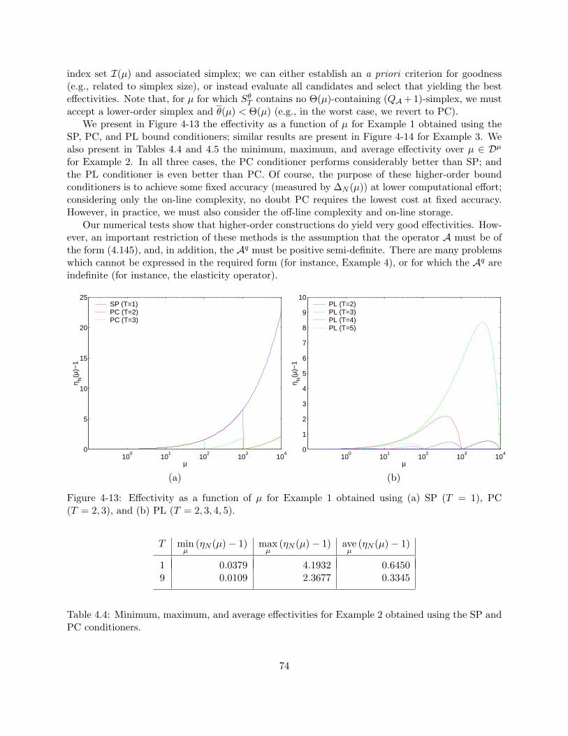
index set I(µ) and associated simplex; we can either establish an a priori criterion for goodness(e.g., related to simplex size), or instead evaluate all candidates and select that yielding the besteffectivities. Note that, for µ for which Sθ

T contains no Θ(µ)-containing (QA+1)-simplex, we mustaccept a lower-order simplex and θ(µ) < Θ(µ) (e.g., in the worst case, we revert to PC).

We present in Figure 4-13 the effectivity as a function of µ for Example 1 obtained using theSP, PC, and PL bound conditioners; similar results are present in Figure 4-14 for Example 3. Wealso present in Tables 4.4 and 4.5 the minimum, maximum, and average effectivity over µ ∈ Dµ

for Example 2. In all three cases, the PC conditioner performs considerably better than SP; andthe PL conditioner is even better than PC. Of course, the purpose of these higher-order boundconditioners is to achieve some fixed accuracy (measured by ∆N (µ)) at lower computational effort;considering only the on-line complexity, no doubt PC requires the lowest cost at fixed accuracy.However, in practice, we must also consider the off-line complexity and on-line storage.

Our numerical tests show that higher-order constructions do yield very good effectivities. How-ever, an important restriction of these methods is the assumption that the operator A must be ofthe form (4.145), and, in addition, the Aq must be positive semi-definite. There are many problemswhich cannot be expressed in the required form (for instance, Example 4), or for which the Aq areindefinite (for instance, the elasticity operator).

100

101

102

103

104

0

5

10

15

20

25

µ

η N(µ

)−1

SP (T=1)PC (T=2)PC (T=3)

(a)

100

101

102

103

104

0

1

2

3

4

5

6

7

8

9

10

µ

η N(µ

)−1

PL (T=2)PL (T=3)PL (T=4)PL (T=5)

(b)

Figure 4-13: Effectivity as a function of µ for Example 1 obtained using (a) SP (T = 1), PC(T = 2, 3), and (b) PL (T = 2, 3, 4, 5).

T minµ

(ηN (µ)− 1) maxµ

(ηN (µ)− 1) aveµ

(ηN (µ)− 1)

1 0.0379 4.1932 0.64509 0.0109 2.3677 0.3345

Table 4.4: Minimum, maximum, and average effectivities for Example 2 obtained using the SP andPC conditioners.

74

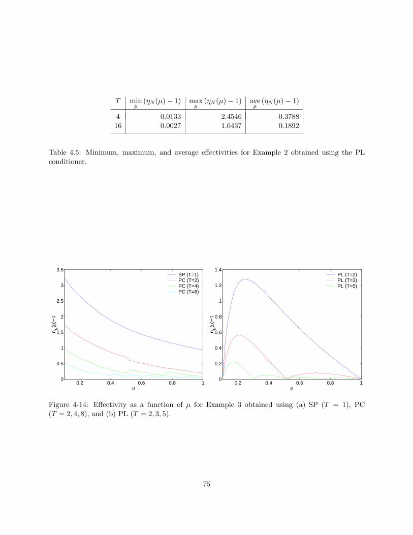
T minµ

(ηN (µ)− 1) maxµ

(ηN (µ)− 1) aveµ

(ηN (µ)− 1)

4 0.0133 2.4546 0.378816 0.0027 1.6437 0.1892

Table 4.5: Minimum, maximum, and average effectivities for Example 2 obtained using the PLconditioner.

0.2 0.4 0.6 0.8 10

0.5

1

1.5

2

2.5

3

3.5

µ

η N(µ

)−1

SP (T=1)PC (T=2)PC (T=4)PC (T=8)

0.2 0.4 0.6 0.8 10

0.2

0.4

0.6

0.8

1

1.2

1.4

µ

η N(µ

)−1

PL (T=2)PL (T=3)PL (T=5)

Figure 4-14: Effectivity as a function of µ for Example 3 obtained using (a) SP (T = 1), PC(T = 2, 4, 8), and (b) PL (T = 2, 3, 5).

75

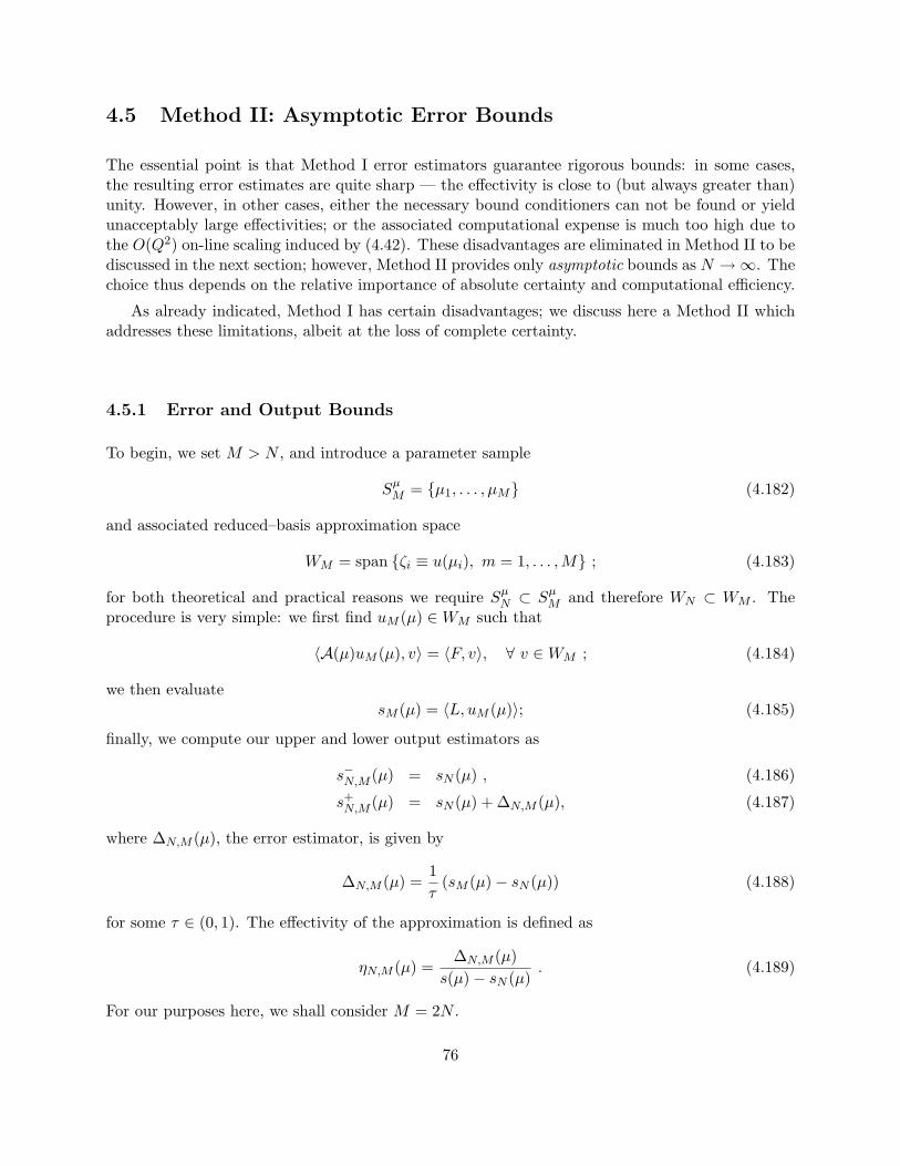
4.5 Method II: Asymptotic Error Bounds

The essential point is that Method I error estimators guarantee rigorous bounds: in some cases,the resulting error estimates are quite sharp — the effectivity is close to (but always greater than)unity. However, in other cases, either the necessary bound conditioners can not be found or yieldunacceptably large effectivities; or the associated computational expense is much too high due tothe O(Q2) on-line scaling induced by (4.42). These disadvantages are eliminated in Method II to bediscussed in the next section; however, Method II provides only asymptotic bounds as N →∞. Thechoice thus depends on the relative importance of absolute certainty and computational efficiency.

As already indicated, Method I has certain disadvantages; we discuss here a Method II whichaddresses these limitations, albeit at the loss of complete certainty.

4.5.1 Error and Output Bounds

To begin, we set M > N , and introduce a parameter sample

SµM = µ1, . . . , µM (4.182)

and associated reduced–basis approximation space

WM = span ζi ≡ u(µi), m = 1, . . . ,M ; (4.183)

for both theoretical and practical reasons we require SµN ⊂ Sµ

M and therefore WN ⊂ WM . Theprocedure is very simple: we first find uM (µ) ∈WM such that

〈A(µ)uM (µ), v〉 = 〈F, v〉, ∀ v ∈WM ; (4.184)

we then evaluatesM (µ) = 〈L, uM (µ)〉; (4.185)

finally, we compute our upper and lower output estimators as

s−N,M (µ) = sN (µ) , (4.186)

s+N,M (µ) = sN (µ) + ∆N,M (µ), (4.187)

where ∆N,M (µ), the error estimator, is given by

∆N,M (µ) =1τ

(sM (µ)− sN (µ)) (4.188)

for some τ ∈ (0, 1). The effectivity of the approximation is defined as

ηN,M (µ) =∆N,M (µ)

s(µ)− sN (µ). (4.189)

For our purposes here, we shall consider M = 2N .

76

4.5.2 Bounding Properties

As in Section 4.2, we would like to be able to prove the effectivity inequality 1 ≤ ηN,2N (µ) ≤ ρ, forall N ≥ 1. However, we can only demonstrate an asymptotic form of this inequality [39].

As in [39], we shall require the hypothesis that

EN,2N (µ) ≡ s(µ)− s2N (µ)s(µ)− sN (µ)

→ 0, as N →∞. (4.190)

We note that the assumption (4.190) is certainly plausible: if the (a priori) exponential convergenceof (3.105) in fact reflects general asymptotic behavior of the reduced basis approximation, then

s(µ)− sN (µ) ∼ c1e−c2N , (4.191)

s(µ)− s2N (µ) ∼ c1e−2c2N , (4.192)

and henceEN,2N (µ) ∼ e−c2N , (4.193)

as desired.

We first prove the lower effectivity inequality, ηN,M (µ) ≥ 1, which is equivalent to

s−N,2N (µ) ≤ s(µ) ≤ s+N,2N (µ), N →∞. (4.194)

The lower bound property s−N,2N (µ) ≤ s(µ) directly follows from (4.25); indeed, this result stillobtains for all N . To demonstrate the upper bound, we write

s+N,2N (µ) = s+(

1τ− 1)

(s(µ)− sN (µ))− 1τ(s(µ)− s2N (µ)) (4.195)

= s+(

1τ

(1− EN,2N (µ))− 1)

(s(µ)− sN (µ)). (4.196)

Since s(µ)− sN (µ) ≥ 0, and 0 < τ < 1, it follows from (4.190) and (4.196) that there exists a finiteN∗(τ) such that

1− EN,2N (µ) ≥ τ , ∀ N > N∗; (4.197)

it follows thats+N,2N (µ) ≥ s(µ) , ∀ N > N∗ . (4.198)

We therefore obtain asymptotic bounds.

We now investigate the sharpness of our bounds by proving the upper effectivity inequality,ηN,2N (µ) ≤ ρ. From the definitions of ηN,2N (µ), ∆N,2N (µ), and EN,2N (µ), we directly obtain

ηN,2N (µ) =1τ

s2N (µ)− sN (µ)s(µ)− sN (µ)

(4.199)

=1τ

(s2N (µ)− s(µ))− (sN (µ)− s(µ))(s(µ)− sN (µ))

(4.200)

=1τ(1− EN,2N (µ)). (4.201)

77

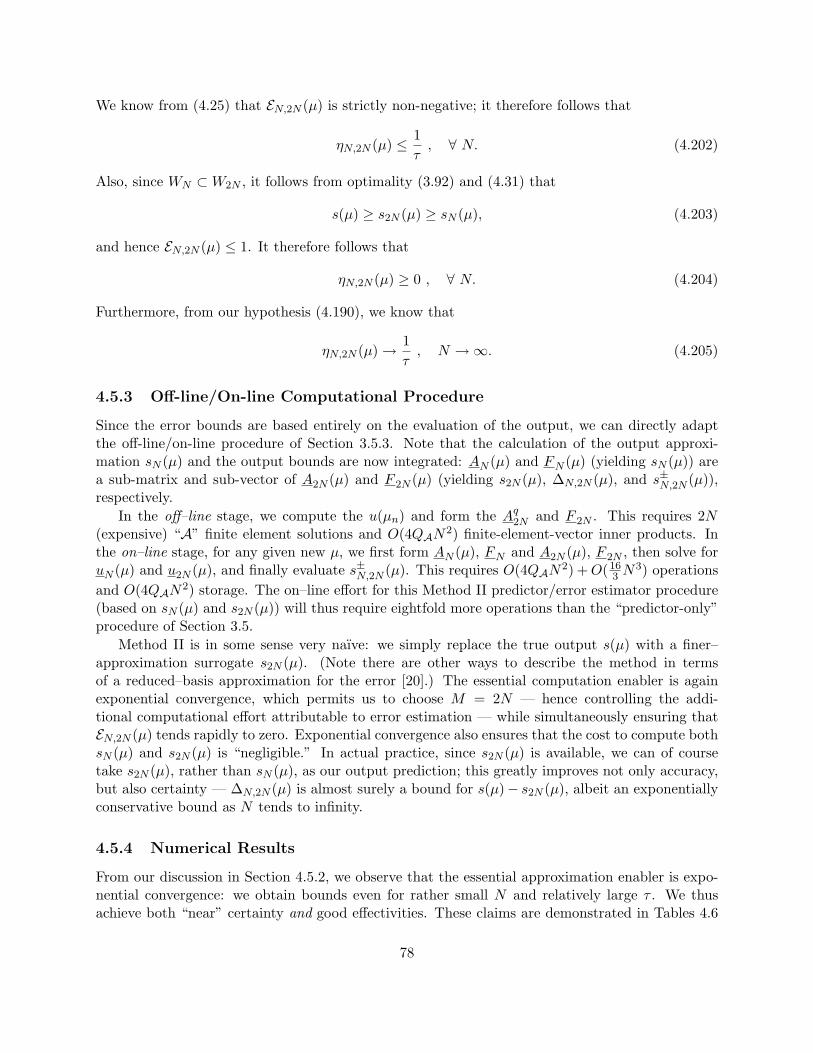
We know from (4.25) that EN,2N (µ) is strictly non-negative; it therefore follows that

ηN,2N (µ) ≤ 1τ, ∀ N. (4.202)

Also, since WN ⊂W2N , it follows from optimality (3.92) and (4.31) that

s(µ) ≥ s2N (µ) ≥ sN (µ), (4.203)

and hence EN,2N (µ) ≤ 1. It therefore follows that

ηN,2N (µ) ≥ 0 , ∀ N. (4.204)

Furthermore, from our hypothesis (4.190), we know that

ηN,2N (µ) → 1τ, N →∞. (4.205)

4.5.3 Off-line/On-line Computational Procedure

Since the error bounds are based entirely on the evaluation of the output, we can directly adaptthe off-line/on-line procedure of Section 3.5.3. Note that the calculation of the output approxi-mation sN (µ) and the output bounds are now integrated: AN (µ) and FN (µ) (yielding sN (µ)) area sub-matrix and sub-vector of A2N (µ) and F 2N (µ) (yielding s2N (µ), ∆N,2N (µ), and s±N,2N (µ)),respectively.

In the off–line stage, we compute the u(µn) and form the Aq2N and F 2N . This requires 2N

(expensive) “A” finite element solutions and O(4QAN2) finite-element-vector inner products. Inthe on–line stage, for any given new µ, we first form AN (µ), FN and A2N (µ), F 2N , then solve foruN (µ) and u2N (µ), and finally evaluate s±N,2N (µ). This requires O(4QAN2) +O(16

3 N3) operations

and O(4QAN2) storage. The on–line effort for this Method II predictor/error estimator procedure(based on sN (µ) and s2N (µ)) will thus require eightfold more operations than the “predictor-only”procedure of Section 3.5.

Method II is in some sense very naıve: we simply replace the true output s(µ) with a finer–approximation surrogate s2N (µ). (Note there are other ways to describe the method in termsof a reduced–basis approximation for the error [20].) The essential computation enabler is againexponential convergence, which permits us to choose M = 2N — hence controlling the addi-tional computational effort attributable to error estimation — while simultaneously ensuring thatEN,2N (µ) tends rapidly to zero. Exponential convergence also ensures that the cost to compute bothsN (µ) and s2N (µ) is “negligible.” In actual practice, since s2N (µ) is available, we can of coursetake s2N (µ), rather than sN (µ), as our output prediction; this greatly improves not only accuracy,but also certainty — ∆N,2N (µ) is almost surely a bound for s(µ)− s2N (µ), albeit an exponentiallyconservative bound as N tends to infinity.

4.5.4 Numerical Results

From our discussion in Section 4.5.2, we observe that the essential approximation enabler is expo-nential convergence: we obtain bounds even for rather small N and relatively large τ . We thusachieve both “near” certainty and good effectivities. These claims are demonstrated in Tables 4.6

78

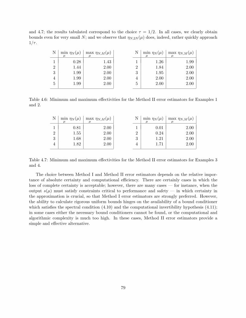
and 4.7; the results tabulated correspond to the choice τ = 1/2. In all cases, we clearly obtainbounds even for very small N ; and we observe that ηN,2N (µ) does, indeed, rather quickly approach1/τ .

N minµ

ηN (µ) maxµ

ηN,M (µ)

1 0.28 1.432 1.44 2.003 1.99 2.004 1.99 2.005 1.99 2.00

N minµ

ηN (µ) maxµ

ηN,M (µ)

1 1.26 1.992 1.84 2.003 1.95 2.004 2.00 2.005 2.00 2.00

Table 4.6: Minimum and maximum effectivities for the Method II error estimators for Examples 1and 2.

N minµ

ηN (µ) maxµ

ηN,M (µ)

1 0.81 2.002 1.55 2.003 1.68 2.004 1.82 2.00

N minµ

ηN (µ) maxµ

ηN,M (µ)

1 0.01 2.002 0.24 2.003 1.21 2.004 1.71 2.00

Table 4.7: Minimum and maximum effectivities for the Method II error estimators for Examples 3and 4.

The choice between Method I and Method II error estimators depends on the relative impor-tance of absolute certainty and computational efficiency. There are certainly cases in which theloss of complete certainty is acceptable; however, there are many cases — for instance, when theoutput s(µ) must satisfy constraints critical to performance and safety — in which certainty inthe approximation is crucial, so that Method I error estimators are strongly preferred. However,the ability to calculate rigorous uniform bounds hinges on the availability of a bound conditionerwhich satisfies the spectral condition (4.10) and the computational invertibility hypothesis (4.11);in some cases either the necessary bound conditioners cannot be found, or the computational andalgorithmic complexity is much too high. In these cases, Method II error estimators provide asimple and effective alternative.

79

80

Chapter 5

Reduced-Basis Output Bounds forLinear Elasticity and NoncompliantOutputs

5.1 Introduction

In Chapter 3 we present the reduced basis method for approximating compliant linear functionaloutputs associated with elliptic partial differential equations. In Chapter 4, we develop two generalapproaches for a posteriori error estimation: Method I, which provides rigorous uniform errorbounds obtained from relaxations of the error residual equation; and Method II, which providesasymptotic error bounds obtained from “finer” reduced basis approximations. In both chapters,we utilize several simple problems in steady-state heat conduction to illustrate our methods andnumerically verify our claims.

In this chapter, we apply reduced basis approximation and error estimation methods to linearelasticity. The problem of linear elasticity brings about some challenging but important issues:first, a decidedly more complex parametric dependence — related to the affine decomposition ofthe operator — causes an increase in the required computational expense and storage; and second,singularities in the elasticity tensor associated with pure-rotation modes — related to the coercivityconstant of the operator — causes the effectivity of the error estimators in certain cases to beunacceptably high.

Furthermore, in Chapters 3 and 4 the methods are restricted to compliant parameter-independentoutputs, L = F . We formulate here the reduced-basis method and associated error estimation pro-cedures for more general linear bounded output functionals.

5.2 Abstraction

As in Chapter 3, we consider a suitably regular (smooth) parameter-independent domain Ω ⊂IRd, d = 1, 2, or 3, and associated function space Y ⊂ (H1(Ω))p with inner product (·, ·)Y , norm|| · ||Y = (·, ·)1/2

Y , dual space Y ′, and duality pairing 〈 ·, ·〉 = Y ′〈 ·, ·〉Y ; as before, we define aparameter set Dµ ⊂ IRP , a particular point in which will be denoted µ.

We now consider the symmetric, continuous, and coercive distributional (second-order partial

81

differential) operator A(µ) : Y → Y ′, and introduce the bounded linear forms F (µ) ∈ Y ′ andL(µ) ∈ Y ′; note we no longer assume that L = F . We shall again make certain assumptions onthe parametric dependence of A, F , and L. In particular, we shall suppose that, for some finite(preferably small) integers QA, QF , and QL, A(µ), F (µ), and L(µ) may be expressed as

A(µ) =QA∑q=1

Θq(µ)Aq , ∀ µ ∈ Dµ , (5.1)

F (µ) =QF∑q=1

ϕqF (µ) F q , ∀ µ ∈ Dµ , (5.2)

L(µ) =QL∑q=1

ϕqL(µ) Lq , ∀ µ ∈ Dµ , (5.3)

where the Θq(µ) : Dµ → IR, ϕqF (µ) : Dµ → IR, ϕq

L(µ) : Dµ → IR, Aq : Y → Y ′, F q ∈ Y ′, and Lq ∈ Y ′.As earlier indicated, this assumption of “separability” or affine parameter dependence is crucial tocomputational efficiency.

Our abstract problem statement is then: for any µ ∈ Dµ ⊂ IRP , find s(µ) ∈ IR given by

s(µ) = 〈L(µ), u(µ)〉, (5.4)

where u(µ) ∈ Y is the solution of

〈A(µ)u(µ), v〉 = 〈F (µ), v〉, ∀ v ∈ Y. (5.5)

Thus, (5.5) is our partial differential equation (in weak form), µ is our parameter, u(µ) is our fieldvariable, and s(µ) is our output.

In actual practice, Y is replaced by an appropriate “truth” finite element approximation spaceYN of dimension N defined on a suitably fine truth mesh. We then approximate u(µ) and s(µ) byuN (µ) and sN (µ), respectively, and assume that YN is sufficiently rich such that uN (µ) and sN (µ)are indistinguishable from u(µ) and s(µ).

5.3 Formulation of the Linear Elasticity Problem

In this section we present the strong form of the equations of linear elasticity, from which wederive the weak statement; we then reformulate the problem in terms of a reference (parameter-independent) domain, thus recovering the abstract formulation of Section 5.2. In this and thefollowing sections, repeated indices imply summation, and, unless otherwise indicated, indices takeon the values 1 through d, where d is the dimensionality of the problem. Furthermore, in thissection we use a bar to signify a general dependence on the parameter µ (e.g., Ω ≡ Ω(µ), or E ≡ µ)particularly when formulating the problem in a “non-reference”domain.

5.3.1 Governing Equations

For simplicity of exposition, we present the governing equations for the case of a homogeneousbody, and merely state the weak statement for the more general case of an inhomogeneous body.

82

Strong Formulation

We consider the deformation of a homogeneous body Ω ⊂ IRd with boundary Γ subjected to externalbody forces, surface tractions and homogeneous displacement boundary conditions. We assume thatthe displacement gradients are sufficiently small that a linear elasticity model adequately describesthe deformation; in particular, we assume that the equations of equilibrium are satisfied in theundeformed configuration

∂σij

∂xj+ bi = 0 in Ω , (5.6)

and the stresses σij are related to the linearized strains εij by the constitutive equations

σij = Cijklεkl , (5.7)

where the linearized strains are related to the displacements u by

εkl =12

(∂uk

∂xl+∂ul

∂xk

). (5.8)

Assuming the material is isotropic1, the elasticity tensor has the form

Cijkl = c1δijδkl + c2 (δikδjl + δilδjk) ; (5.9)

we note that from the symmetry of σij and εkl, and from isotropy, the elasticity tensor satisfies

Cijkl = Cjikl = Cijlk = Cklij , (5.10)

from which it follows thatσij = Cijkl

∂uk

∂xl, (5.11)

Here, c1 and c2 are Lame’s constants, related to Young’s modulus, E, and Poisson’s ratio, ν, by

c1 =Eν

(1 + ν)(1− 2ν), (5.12)

c2 =E

2(1 + ν). (5.13)

The displacement and traction boundary conditions are given by

uieni = 0 , on Γn

D , (5.14)uiet

i = 0 , on ΓtD , (5.15)

1Note the assumption of isotropy is introduced only for simplicity — the methods we develop are similarly appli-cable to general anisotropic materials so long as the spatial and parametric dependence of the elasticity tensor areseparable, i.e., Cijkl(x; µ) = ¯f(x) ¯Cijkl(µ).

83

and

σij enj =

fnen

i on ΓnN

0 on Γ\(ΓnD ∪ Γn

N)(5.16)

σij enj =

ftet

i on ΓtN

0 on Γ\(ΓtD ∪ Γt

N) ,(5.17)

respectively, where eni and et

i are the unit normal and tangent vectors on Γ.

Weak Formulation

We now derive the weak form of the governing equations. To begin, we introduce the functionspace

Y = v ∈(H1(Ω)

)p=d | vieni = 0 on Γn

D, vieti = 0 on Γt

D , (5.18)

and associated norm

||v||Y =

(d∑

i=1

||vi||2H1(Ω)

)1/2

=

∫Ω

d∑i,j=1

(∂vi

∂xj

)2

dΩ

1/2

. (5.19)

Multiplying (5.6) by a test function v ∈ Y and integrating over Ω, we obtain

−∫

Ωvi∂σij

∂xjdΩ =

∫Ωbivi dΩ , ∀ v ∈ Y . (5.20)

Integrating by parts and applying the divergence theorem yields

−∫

Ωvi∂σij

∂xjdΩ = −

∫Γviσij en

j dΓ +∫

Ω

∂vi

∂xjσij dΩ , ∀ v ∈ Y . (5.21)

Substituting (5.21) into (5.20), and using (5.14), (5.16), and the fact that v ∈ Y , we find that∫Ω

∂vi

∂xjσij dΩ =

∫Ωvibi dΩ +

∫Γn

N

vifneni dΓ +

∫Γt

N

vifteti dΓ . (5.22)

Finally, using (5.11), we obtain as our weak statement

〈Au, v〉 = 〈F , v〉 , ∀ v ∈ Y , (5.23)

where

〈Aw, v〉 =∫

Ω

∂vi

∂xjCijkl

∂wk

∂xl(5.24)

〈F , v〉 = 〈Ff , v〉+ 〈Fb, v〉 ; (5.25)

here,

〈Ff , v〉 =∫

ΓnN

vifneni dΓ +

∫Γt

N

vifteti dΓ , 〈Fb, v〉 =

∫Ωvibi dΩ . (5.26)

84

We now generalize (5.23)-(5.26) to the case in which Ω is inhomogeneous. Assuming that Ωconsists of R homogeneous subdomains Ωr such that

Ω =R⋃

r=1

Ωr , (5.27)

the weak statement takes the form of (5.23) where

〈Aw, v〉 =R∑

r=1

∫Ωr

∂vi

∂xjC r

ijkl

∂wk

∂xldΩ (5.28)

〈F , v〉 = 〈Ff , v〉+ 〈Fb, v〉 , (5.29)

and

〈Fb, v〉 =R∑

r=1

∫Ωr

vibri dΩ , 〈Ff , v〉 =

R∑r=1

(∫Γn r

N

vifrnen

i dΓ +∫

Γt rN

vifrt et

i dΓ

); (5.30)

here, Ω is the closure of Ω, C rijkl is the elasticity tensor in Ωr, and Γr

N is the section of ΓN in Ωr. The

derivation of (5.28)-(5.30) is similar to that for the homogeneous case, but for the use of additionaldisplacement and traction continuity conditions at the interfaces between the Ωr.

5.3.2 Reduction to Abstract Form

In this section, we reformulate the problem defined by (5.28)-(5.30) so as to recover the abstractformulation of Section 5.2.

Affine Geometric Mapping

As before, we further partition the subdomains Ωr, r = 1, . . . , R, into a total of R subdomainsΩr, r = 1, . . . , R such that there exists a reference domain Ω =

⋃Rr=1 Ωr where, for any x ∈ Ωr,

r = 1, . . . , R, its image x ∈ Ωr is given by

x = Gr(µ; x) = Gr(µ)x+ gr(µ); (5.31)

we write∂

∂xi=∂xj

∂xi

∂

∂xj= Gji(µ)

∂

∂xj, (5.32)

andx = G(µ; x) = G(µ)x+ g(µ) , (5.33)

where x ∈ Ω, x ∈ Ω, G(µ) ∈ IRd×d is a piecewise-constant matrix, gr(µ) ∈ IRd is a piecewise-constant vector, and G(µ) : Ω → Ω is a piecewise-affine geometric mapping.

85

Reference Domain Formulation

We now define the function space Y as Y (Ω) = Y (G−1(µ; Ω)) = Y (Ω), i.e.,

Y = v ∈(H1(Ω)

)p=d | vieni = 0 on Γn

D, vieti = 0 on Γt

D , (5.34)

and for any function w ∈ Y , we define w ∈ Y such that w(x) = w(G−1(µ;x)). Furthermore, wehave

dΩ = detG−1(µ) dΩ , (5.35)dΓ =

∣∣G−1(µ) et∣∣ dΓ , (5.36)

where et is a unit vector tangent to the boundary Γ, and

∣∣G−1(µ) et∣∣ = ( d∑

i=1

(Gijet

j

)2)1/2

. (5.37)

It then follows that 〈A(µ)w, v〉 = 〈Aw, v〉 for A as in (5.28) and A(µ) given by

〈A(µ)w, v〉 =R∑

r=1

∫Ωr

(Gr

jj′(µ)∂wi

∂xj

)Er

ij′kl′

(Gr

ll′(µ)∂vk

∂xl

)det(Gr(µ))−1 dΩ , (5.38)

=R∑

r=1

∫Ωr

∂wi

∂xj

(Gr

jj′(µ)Erij′kl′G

rll′(µ) det(G(µ))−1

) ∂vk

∂xldΩ ∀ w, v ∈ Y , (5.39)

and 〈F (µ)w, v〉 = 〈F w, v〉 for F as in (5.29) and F (µ) given by

〈F (µ), v〉 =R∑

r=1

(∫Ωr

(bri det (Gr(µ))−1

)vi dΩ +

∫Γn r

N

(f r

neni

∣∣(Gr(µ))−1et∣∣) vi dΓ

+∫

Γt rN

(f r

t eti

∣∣(Gr(µ))−1et∣∣) vi dΓ

). (5.40)

The abstract problem statement of Section 5.2 is then recovered for

〈A(µ)w, v〉 =R∑

r=1

∫Ωr

∂wi

∂xjCr

ijkl(µ)∂vk

∂xl∀ w, v ∈ Y , (5.41)

〈F (µ), v〉 = (〈Fb(µ), v〉+ 〈Ff (µ), v〉) (5.42)

86

where

〈Fb(µ), v〉 =R∑

r=1

∫Ωr

bri (µ)vi (5.43)

〈Ff (µ), v〉 =R∑

r=1

(∫Γn r

N

fn ri (µ)vi dΓ +

∫Γt r

N

f t ri (µ)vi dΓ

); (5.44)

here Crijkl(µ) is given by

Crijkl(µ) = Gr

jj′(µ) Erij′kl′ G

rll′(µ) det(Gr(µ))−1 , (5.45)

and bri (µ), fn ri (µ), and f t r

i (µ) are given by

bri (µ) = bri det (Gr(µ))−1 , (5.46)fn r

i (µ) = f rnen

i

∣∣(Gr(µ))−1et∣∣ , (5.47)

f t ri (µ) = f r

t eti

∣∣(Gr(µ))−1et∣∣ . (5.48)

Furthermore, we define

Θq(i,j,k,l,r)(µ) = Crijkl(µ), 〈Aq(i,j,k,l,r)w, v〉 =

∫Ω

∂vi

∂xj

∂wk

∂xl(5.49)

for i, j, k, l ∈ 1, . . . , d, 1 ≤ r ≤ R, and q : 1, . . . , d4 × 1, . . . , R → 1, . . . , QA; and

ϕq′(i,r,χ)F =

bri (µ) for χ = 1 ,

fn ri (µ) for χ = 2 ,

f t ri (µ) for χ = 3 ,

F q(i,r,χ) =

∫Ωr

vi for χ = 1 ,∫Γn r

N

vi for χ = 2 ,∫Γt r

N

vi for χ = 3 ,

(5.50)

for 1 ≤ i ≤ d, 1 ≤ r ≤ R, and q′ : 1, . . . , d × 1, . . . , R → 1, . . . , QF . Note however thatdue to the symmetry of Cijkl(µ), QA can in fact be taken to be d2(d2 + 1)R/2 rather than d4R;furthermore, QA and QF can be further reduced by eliminating the elements of Cijkl(µ) which areidentically zero. This is illustrated in the model problems to be discussed in the following section.

5.4 Model Problems

We indicate here several simple instantiations of the linear elasticity problem; these examples willserve to illustrate our assumptions and methods, and show ways in which the affine parameterdependence may be further simplified.

87

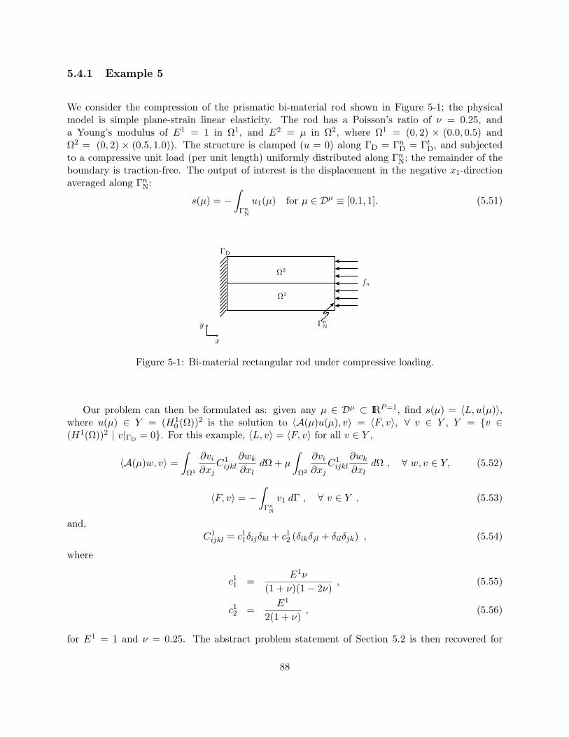
5.4.1 Example 5

We consider the compression of the prismatic bi-material rod shown in Figure 5-1; the physicalmodel is simple plane-strain linear elasticity. The rod has a Poisson’s ratio of ν = 0.25, anda Young’s modulus of E1 = 1 in Ω1, and E2 = µ in Ω2, where Ω1 = (0, 2) × (0.0, 0.5) andΩ2 = (0, 2) × (0.5, 1.0)). The structure is clamped (u = 0) along ΓD = Γn

D = ΓtD, and subjected

to a compressive unit load (per unit length) uniformly distributed along ΓnN; the remainder of the

boundary is traction-free. The output of interest is the displacement in the negative x1-directionaveraged along Γn

N:

s(µ) = −∫

ΓnN

u1(µ) for µ ∈ Dµ ≡ [0.1, 1]. (5.51)

ΓD

fn

ΓnNy

x

Ω1

Ω2

Figure 5-1: Bi-material rectangular rod under compressive loading.

Our problem can then be formulated as: given any µ ∈ Dµ ⊂ IRP=1, find s(µ) = 〈L, u(µ)〉,where u(µ) ∈ Y = (H1

0 (Ω))2 is the solution to 〈A(µ)u(µ), v〉 = 〈F, v〉, ∀ v ∈ Y , Y = v ∈(H1(Ω))2 | v|ΓD

= 0. For this example, 〈L, v〉 = 〈F, v〉 for all v ∈ Y ,

〈A(µ)w, v〉 =∫

Ω1

∂vi

∂xjC1

ijkl

∂wk

∂xldΩ + µ

∫Ω2

∂vi

∂xjC1

ijkl

∂wk

∂xldΩ , ∀ w, v ∈ Y, (5.52)

〈F, v〉 = −∫

ΓnN

v1 dΓ , ∀ v ∈ Y , (5.53)

and,C1

ijkl = c11δijδkl + c12 (δikδjl + δilδjk) , (5.54)

where

c11 =E1ν

(1 + ν)(1− 2ν), (5.55)

c12 =E1

2(1 + ν), (5.56)

for E1 = 1 and ν = 0.25. The abstract problem statement of Section 5.2 is then recovered for

88

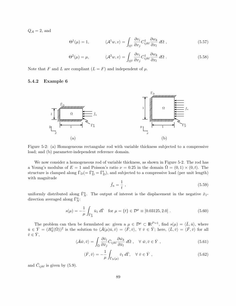
QA = 2, and

Θ1(µ) = 1, 〈A1w, v〉 =∫

Ω1

∂vi

∂xjC1

ijkl

∂wk

∂xldΩ , (5.57)

Θ2(µ) = µ, 〈A2w, v〉 =∫

Ω2

∂vi

∂xjC1

ijkl

∂wk

∂xldΩ . (5.58)

Note that F and L are compliant (L = F ) and independent of µ.

5.4.2 Example 6

t

y

x

1

Ω

ΓD

fn

ΓnN

(a)

fn

ΓD

ΓnN

1

1

Ω

y

x

(b)

Figure 5-2: (a) Homogeneous rectangular rod with variable thickness subjected to a compressiveload; and (b) parameter-independent reference domain.

We now consider a homogeneous rod of variable thickness, as shown in Figure 5-2. The rod hasa Young’s modulus of E = 1 and Poisson’s ratio ν = 0.25 in the domain Ω = (0, 1) × (0, t). Thestructure is clamped along ΓD(= Γn

D = ΓtD), and subjected to a compressive load (per unit length)

with magnitude

fn =1t, (5.59)

uniformly distributed along ΓnN. The output of interest is the displacement in the negative x1-

direction averaged along ΓnN:

s(µ) = − 1µ

∫Γn

N

u1 dΓ for µ = t ∈ Dµ ≡ [0.03125, 2.0] . (5.60)

The problem can then be formulated as: given a µ ∈ Dµ ⊂ IRP=1, find s(µ) = 〈L, u〉, whereu ∈ Y = (H1

0 (Ω))2 is the solution to 〈A(µ)u, v〉 = 〈F , v〉, ∀ v ∈ Y ; here, 〈L, v〉 = 〈F , v〉 for allv ∈ Y ,

〈Aw, v〉 =∫

Ω

∂vi

∂xjCijkl

∂wk

∂xldΩ , ∀ w, v ∈ Y , (5.61)

〈F , v〉 = − 1µ

∫ΓN(µ)

v1 dΓ, ∀ v ∈ Y , (5.62)

and Cijkl is given by (5.9).

89

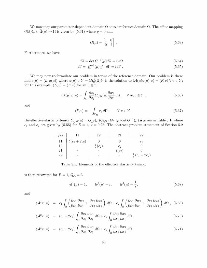
We now map our parameter-dependent domain Ω onto a reference domain Ω. The affine mappingG(x)(µ) : Ω(µ) → Ω is given by (5.31) where g = 0 and

G(µ) =[1 00 1

t

]. (5.63)

Furthermore, we have

dΩ = detG−1(µ)dΩ = t dΩ (5.64)dΓ =

∣∣G−1(µ) et∣∣ dΓ = tdΓ . (5.65)

We may now re-formulate our problem in terms of the reference domain. Our problem is then:find s(µ) = 〈L, u(µ)〉 where u(µ) ∈ Y = (H1

0 (Ω))2 is the solution to 〈A(µ)u(µ), v〉 = 〈F, v〉 ∀ v ∈ Y ;for this example, 〈L, v〉 = 〈F, v〉 for all v ∈ Y,

〈A(µ)w, v〉 =∫

Ω

∂vi

∂xjCijkl(µ)

∂wk

∂xldΩ , ∀ w, v ∈ Y , (5.66)

and〈F, v〉 = −

∫ΓN

v1 dΓ , ∀ v ∈ Y ; (5.67)

the effective elasticity tensor Cijkl(µ) = Gjj′(µ)Cij′kl′Gll′(µ) detG−1(µ) is given in Table 5.1, wherec1 and c2 are given by (5.55) for E = 1, ν = 0.25. The abstract problem statement of Section 5.2

ij\kl 11 12 21 22

11 t (c1 + 2c2) 0 0 c112 · 1

t (c2) c2 021 · · t(c2) 022 · · · 1

t (c1 + 2c2)

Table 5.1: Elements of the effective elasticity tensor.

is then recovered for P = 1, QA = 3,

Θ1(µ) = 1, Θ2(µ) = t, Θ3(µ) =1t, (5.68)

and

〈A1w, v〉 = c1

∫Ω

(∂v1∂x1

∂w2

∂x2+∂v2∂x2

∂w1

∂x1

)dΩ + c2

∫Ω

(∂v1∂x2

∂w2

∂x1+∂v2∂x1

∂w1

∂x2

)dΩ , (5.69)

〈A2w, v〉 = (c1 + 2c2)∫

Ω

∂v1∂x1

∂w1

∂x1dΩ + c2

∫Ω

∂v2∂x1

∂w2

∂x1dΩ , (5.70)

〈A3w, v〉 = (c1 + 2c2)∫

Ω

∂v2∂x2

∂w2

∂x2dΩ + c2

∫Ω

∂v1∂x2

∂w1

∂x2dΩ . (5.71)

90

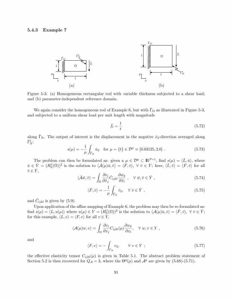
5.4.3 Example 7

ΓD

ΓtN

Ωft

1x

y

t

(a)

ΓD

1

y

x

1

ftΩ

ΓtN

(b)

Figure 5-3: (a) Homogeneous rectangular rod with variable thickness subjected to a shear load;and (b) parameter-independent reference domain.

We again consider the homogeneous rod of Example 6, but with ΓD as illustrated in Figure 5-3,and subjected to a uniform shear load per unit length with magnitude

ft =1t

(5.72)

along ΓN. The output of interest is the displacement in the negative x2-direction averaged alongΓt

N:

s(µ) = − 1µ

∫ΓN

u2 for µ = t ∈ Dµ ≡ [0.03125, 2.0] . (5.73)

The problem can then be formulated as: given a µ ∈ Dµ ⊂ IRP=1, find s(µ) = 〈L, u〉, whereu ∈ Y = (H1

0 (Ω))2 is the solution to 〈A(µ)u, v〉 = 〈F , v〉, ∀ v ∈ Y ; here, 〈L, v〉 = 〈F , v〉 for allv ∈ Y ,

〈Aw, v〉 =∫

Ω

∂vi

∂xjCijkl

∂wk

∂xl, ∀ w, v ∈ Y , (5.74)

〈F , v〉 = − 1µ

∫ΓN

v2, ∀ v ∈ Y , (5.75)

and Cijkl is given by (5.9).Upon application of the affine mapping of Example 6, the problem may then be re-formulated as:

find s(µ) = 〈L, u(µ)〉 where u(µ) ∈ Y = (H10 (Ω))2 is the solution to 〈A(µ)u, v〉 = 〈F , v〉, ∀ v ∈ Y ;

for this example, 〈L, v〉 = 〈F, v〉 for all v ∈ Y,

〈A(µ)w, v〉 =∫

Ω

∂vi

∂xjCijkl(µ)

∂wk

∂xl, ∀ w, v ∈ Y , (5.76)

and〈F, v〉 = −

∫ΓN

v2, ∀ v ∈ Y ; (5.77)

the effective elasticity tensor Cijkl(µ) is given in Table 5.1. The abstract problem statement ofSection 5.2 is then recovered for QA = 3, where the Θq(µ) and Aq are given by (5.68)-(5.71).

91

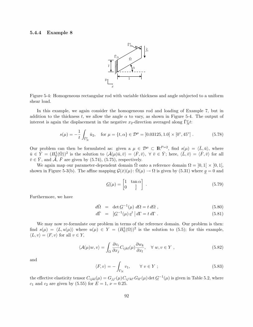
5.4.4 Example 8

ΓD

t

y

x

1

α

Ω

ft

ΓtN

Figure 5-4: Homogeneous rectangular rod with variable thickness and angle subjected to a uniformshear load.

In this example, we again consider the homogeneous rod and loading of Example 7, but inaddition to the thickness t, we allow the angle α to vary, as shown in Figure 5-4. The output ofinterest is again the displacement in the negative x2-direction averaged along Γx

Nt:

s(µ) = −1t

∫Γt

N

u2, for µ = t, α ∈ Dµ = [0.03125, 1.0]× [0, 45] . (5.78)

Our problem can then be formulated as: given a µ ∈ Dµ ⊂ IRP=2, find s(µ) = 〈L, u〉, whereu ∈ Y = (H1

0 (Ω))2 is the solution to 〈A(µ)u, v〉 = 〈F , v〉, ∀ v ∈ Y ; here, 〈L, v〉 = 〈F , v〉 for allv ∈ Y , and A, F are given by (5.74), (5.75), respectively.

We again map our parameter-dependent domain Ω onto a reference domain Ω = ]0, 1[ × ]0, 1[,shown in Figure 5-3(b). The affine mapping G(x)(µ) : Ω(µ) → Ω is given by (5.31) where g = 0 and

G(µ) =[1 tanα0 1

t

]. (5.79)

Furthermore, we have

dΩ = detG−1(µ) dΩ = t dΩ , (5.80)dΓ =

∣∣G−1(µ) et∣∣ dΓ = t dΓ . (5.81)

We may now re-formulate our problem in terms of the reference domain. Our problem is then:find s(µ) = 〈L, u(µ)〉 where u(µ) ∈ Y = (H1

0 (Ω))2 is the solution to (5.5); for this example,〈L, v〉 = 〈F, v〉 for all v ∈ Y,

〈A(µ)w, v〉 =∫

Ω

∂vi

∂xjCijkl(µ)

∂wk

∂xl, ∀ w, v ∈ Y , (5.82)

and〈F, v〉 = −

∫ΓN

v1, ∀ v ∈ Y ; (5.83)

the effective elasticity tensor Cijkl(µ) = Gjj′(µ)Cij′kl′Gll′(µ) detG−1(µ) is given in Table 5.2, wherec1 and c2 are given by (5.55) for E = 1, ν = 0.25.

92

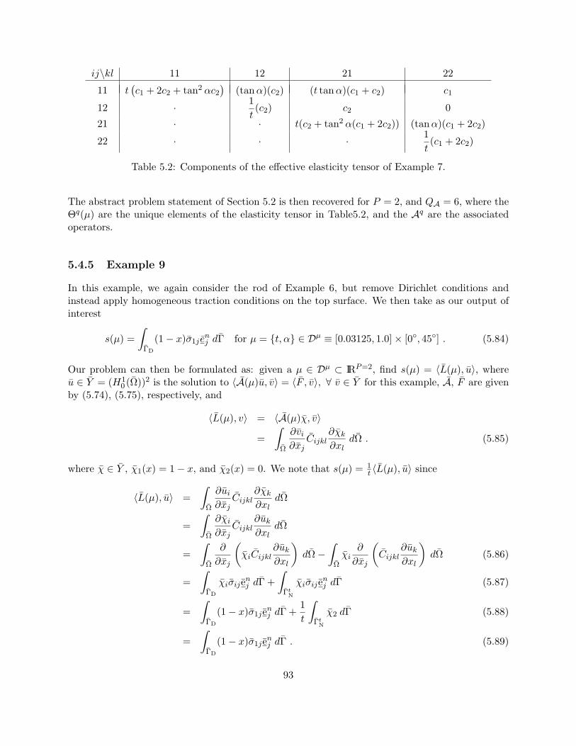
ij\kl 11 12 21 22

11 t(c1 + 2c2 + tan2 αc2

)(tanα)(c2) (t tanα)(c1 + c2) c1

12 · 1t(c2) c2 0

21 · · t(c2 + tan2 α(c1 + 2c2)) (tanα)(c1 + 2c2)

22 · · · 1t(c1 + 2c2)

Table 5.2: Components of the effective elasticity tensor of Example 7.

The abstract problem statement of Section 5.2 is then recovered for P = 2, and QA = 6, where theΘq(µ) are the unique elements of the elasticity tensor in Table5.2, and the Aq are the associatedoperators.

5.4.5 Example 9

In this example, we again consider the rod of Example 6, but remove Dirichlet conditions andinstead apply homogeneous traction conditions on the top surface. We then take as our output ofinterest

s(µ) =∫

ΓD

(1− x)σ1j enj dΓ for µ = t, α ∈ Dµ ≡ [0.03125, 1.0]× [0, 45] . (5.84)

Our problem can then be formulated as: given a µ ∈ Dµ ⊂ IRP=2, find s(µ) = 〈L(µ), u〉, whereu ∈ Y = (H1

0 (Ω))2 is the solution to 〈A(µ)u, v〉 = 〈F , v〉, ∀ v ∈ Y for this example, A, F are givenby (5.74), (5.75), respectively, and

〈L(µ), v〉 = 〈A(µ)χ, v〉

=∫

Ω

∂vi

∂xjCijkl

∂χk

∂xldΩ . (5.85)

where χ ∈ Y , χ1(x) = 1− x, and χ2(x) = 0. We note that s(µ) = 1t 〈L(µ), u〉 since

〈L(µ), u〉 =∫

Ω

∂ui

∂xjCijkl

∂χk

∂xldΩ

=∫

Ω

∂χi

∂xjCijkl

∂uk

∂xldΩ

=∫

Ω

∂

∂xj

(χiCijkl

∂uk

∂xl

)dΩ−

∫Ωχi

∂

∂xj

(Cijkl

∂uk

∂xl

)dΩ (5.86)

=∫

ΓD

χiσij enj dΓ +

∫Γt

N

χiσij enj dΓ (5.87)

=∫

ΓD

(1− x)σ1j enj dΓ +

1t

∫Γt

N

χ2 dΓ (5.88)

=∫

ΓD

(1− x)σ1j enj dΓ . (5.89)

93

We also note that (5.85) is bounded for all v ∈ Y while the more obvious alternative (5.84) is not.

5.5 Reduced-Basis Output Approximation: Compliance

The theoretical basis and general computational procedure presented in Chapter 3 for the reduced-basis approximation of compliant linear functional outputs of interest applies to all problems de-scribed by the abstract formulation of Section 5.2 (or Section 3.2) for the case L = F . We review thecomputational procedure here — this time allowing F to be µ-dependent — and present numericalresults for the linear elasticity model problems of Section 5.4.

5.5.1 Approximation Space

We again introduce a sample in parameter space,

SµN = µ1, . . . , µN (5.90)

where µn ∈ Dµ ⊂ IRP , n = 1, . . . , N , and define our Lagrangian ([37]) reduced-basis approximationspace as

WN = spanζn ≡ u(µn), n = 1, . . . , N, (5.91)

where u(µn) ∈ Y is the solution to (5.5) for µ = µn.

Our reduced-basis approximation is then: for any µ ∈ Dµ, find

sN (µ) = 〈L(µ), uN (µ)〉, (5.92)

where uN (µ) ∈WN is the Galerkin projection of u(µ) onto WN ,

〈A(µ)uN (µ), v〉 = 〈F (µ), v〉, ∀ v ∈WN . (5.93)

5.5.2 Off-line/On-line Computational Procedure

We express our approximation uN (µ) ≈ u(µ) to be a linear combination of the basis functions,

uN (µ) =N∑

j=1

uN j(µ) ζj (5.94)

where uN (µ) ∈ IRN ; we then choose for test functions v = ζi, i = 1, . . . , N . Inserting theserepresentations into (5.93) yields the desired algebraic equations for uN (µ) ∈ IRN ,

AN (µ) uN (µ) = FN (µ) , (5.95)

in terms of which the output can then be evaluated as

sN (µ) = uN (µ)TLN (µ) . (5.96)

Here AN (µ) ∈ IRN×N is the symmetric positive-definite (SPD) matrix with entries

AN i,j(µ) ≡ 〈A(µ)ζj , ζi〉, 1 ≤ i, j ≤ N , (5.97)

94

FN (µ) ∈ IRN is the “load” vector with entries

FN i(µ) ≡ 〈F (µ), ζi〉, 1 ≤ i ≤ N , (5.98)

and LN (µ) = FN (µ). We now invoke (5.1) and (5.2) to write

AN i,j(µ) =QA∑q=1

Θq(µ) 〈Aqζj , ζi〉 , (5.99)

FN i(µ) =QF∑q=1

ϕqF (µ) 〈F q, ζi〉 , (5.100)

or

AN (µ) =QA∑q=1

Θq(µ)AqN , (5.101)

FN (µ) =QF∑q=1

ϕqF (µ) F q

N , (5.102)

where the AqN ∈ IRN×N and F q

N are given by

AqN i,j = 〈Aqζj , ζi〉 , 1 ≤ i, j ≤ N, 1 ≤ q ≤ QA , (5.103)

F qN i = 〈F q, ζi〉 , 1 ≤ i ≤ N, 1 ≤ q ≤ QF . (5.104)

The off-line/on-line decomposition is now clear. In the off-line stage, we compute the u(µn) andform the Aq

N and F qN : this requires N (expensive) “A” finite element solutions, and O(QAN2) +

O(QFN) finite-element-vector (O(N )) inner products. In the on-line stage, for any given newµ, we first form AN (µ) and FN (µ) from (5.101) and (5.102), then solve (5.99) for uN (µ), andfinally evaluate sN (µ) = uN (µ)TFN (µ): this requires O(QAN2 +QFN) +O(2

3N3) operations and

O(QAN2 +QFN) storage.Thus, as required, the incremental, or marginal, cost to evaluate sN (µ) for any given new µ is

very small: first, because N is very small — thanks to the good convergence properties of WN (seeChapter 3); and second, because (5.99) can be very rapidly assembled and inverted — thanks tothe off-line/on-line decomposition. We shall now demonstrate the former by applying our methodsto the compliant model problems of Section 5.4.

5.5.3 Numerical Results

We present in Figures 5-6 to 5-8 the maximum relative error εN (µ) as a function of N for µ ∈ Dµ,for Examples 5 to 8, respectively. In all four cases, the µn are chosen “log-randomly” over Dµ:we sample from a multivariate uniform probability density on log(µ), as described in Chapter 3.We note that the error is monotonically decreasing with N (as predicted by our a priori theory),and even for cases (such as Example 8) for which P > 1, the error is remarkably small evenfor relatively small N . Furthermore, we again observe that the log–random point distributionis important, as evidenced by generally faster convergence (versus the non–logarithmic uniform

95

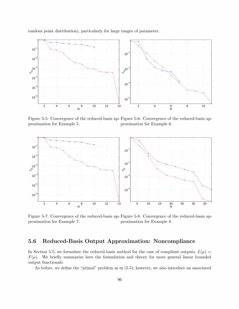
random point distribution), particularly for large ranges of parameter.

2 4 6 8 10 12 14

10−6

10−5

10−4

10−3

10−2

10−1

N

ε N

Figure 5-5: Convergence of the reduced-basis ap-proximation for Example 5.

2 4 6 8 10

10−4

10−3

10−2

10−1

N

ε N

Figure 5-6: Convergence of the reduced-basis ap-proximation for Example 6.

2 4 6 8 10 12 14

10−6

10−5

10−4

10−3

10−2

10−1

N

ε N

Figure 5-7: Convergence of the reduced-basis ap-proximation for Example 7.

5 10 15 20 25 30 35

10−4

10−3

10−2

10−1

N

ε N

Figure 5-8: Convergence of the reduced-basis ap-proximation for Example 8.

5.6 Reduced-Basis Output Approximation: Noncompliance

In Section 5.5, we formulate the reduced-basis method for the case of compliant outputs, L(µ) =F (µ). We briefly summarize here the formulation and theory for more general linear boundedoutput functionals.

As before, we define the “primal” problem as in (5.5); however, we also introduce an associated

96

adjoint or “dual” problem: for any µ ∈ Dµ, find ψ(µ) ∈ Y such that

〈A(µ)v, ψ(µ)〉 = −〈L(µ), v〉 , ∀ v ∈ Y ; (5.105)

recall that L(µ) is our output functional.

5.6.1 Approximation Space

To develop the reduced-basis space, we first choose, randomly or log-randomly as described inChapter 3, a sample set in parameter space,

SµN/2 = µ1, . . . , µN/2 (5.106)

where µn ∈ Dµ ⊂ IRP , n = 1, . . . , N/2; we now consider two approaches — “nonsegregated” and“segregated” — for defining our Lagrangian ([37]) reduced-basis approximation.

Nonsegregated Approach

We define the nonsegregated reduced-basis approximation space as

WN = span u(µn), ψ(µn), n = 1, . . . , N/2 (5.107)≡ span ζn, n = 1, . . . , N (5.108)

where u(µn) ∈ Y and ψ(µn) ∈ Y are the solutions to (5.5) and (5.105), respectively, for µ = µn.

Our reduced-basis approximation is then: for any µ ∈ Dµ, find

sN (µ) = 〈L(µ), uN (µ)〉, (5.109)

where uN (µ) ∈ WN and ψN (µ) ∈ WN are the Galerkin projections of u(µ) and ψ(µ), respectively,onto WN ,

〈A(µ)uN (µ), v〉 = 〈F (µ), v〉, ∀ v ∈WN , (5.110)〈A(µ)ψN (µ), v〉 = −〈L(µ), v〉, ∀ v ∈WN . (5.111)

Turning now to the a priori theory, it follows from standard arguments that uN (µ) and ψN (µ)are “optimal” in the sense that

||u(µ)− uN (µ)||Y ≤

√γA(µ)αA(µ)

infwN∈WN

||u(µ)− wN ||Y , (5.112)

||ψ(µ)− ψN (µ)||Y ≤

√γA(µ)αA(µ)

infwN∈WN

||ψ(µ)− wN ||Y . (5.113)

The proof of (5.112) and the best approximation analysis is similar to that presented in Section 3.5.2.

97

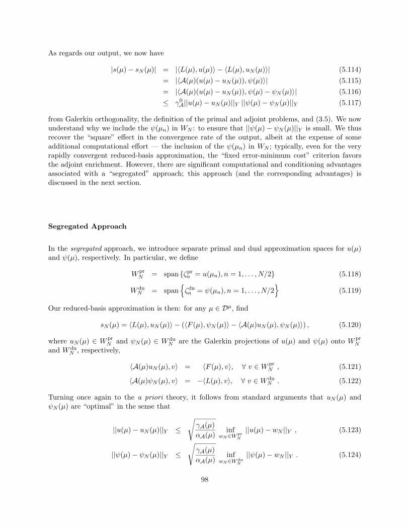
As regards our output, we now have

|s(µ)− sN (µ)| = |〈L(µ), u(µ)〉 − 〈L(µ), uN (µ)〉| (5.114)= |〈A(µ)(u(µ)− uN (µ)), ψ(µ)〉| (5.115)= |〈A(µ)(u(µ)− uN (µ)), ψ(µ)− ψN (µ)〉| (5.116)≤ γ0

A||u(µ)− uN (µ)||Y ||ψ(µ)− ψN (µ)||Y (5.117)

from Galerkin orthogonality, the definition of the primal and adjoint problems, and (3.5). We nowunderstand why we include the ψ(µn) in WN : to ensure that ||ψ(µ)− ψN (µ)||Y is small. We thusrecover the “square” effect in the convergence rate of the output, albeit at the expense of someadditional computational effort — the inclusion of the ψ(µn) in WN ; typically, even for the veryrapidly convergent reduced-basis approximation, the “fixed error-minimum cost” criterion favorsthe adjoint enrichment. However, there are significant computational and conditioning advantagesassociated with a “segregated” approach; this approach (and the corresponding advantages) isdiscussed in the next section.

Segregated Approach

In the segregated approach, we introduce separate primal and dual approximation spaces for u(µ)and ψ(µ), respectively. In particular, we define

W prN = span ζpr

n = u(µn), n = 1, . . . , N/2 (5.118)

W duN = span

ζdun = ψ(µn), n = 1, . . . , N/2

(5.119)

Our reduced-basis approximation is then: for any µ ∈ Dµ, find

sN (µ) = 〈L(µ), uN (µ)〉 − (〈F (µ), ψN (µ)〉 − 〈A(µ)uN (µ), ψN (µ)〉) , (5.120)

where uN (µ) ∈ W prN and ψN (µ) ∈ W du

N are the Galerkin projections of u(µ) and ψ(µ) onto W prN

and W duN , respectively,

〈A(µ)uN (µ), v〉 = 〈F (µ), v〉, ∀ v ∈W prN , (5.121)

〈A(µ)ψN (µ), v〉 = −〈L(µ), v〉, ∀ v ∈W duN . (5.122)

Turning once again to the a priori theory, it follows from standard arguments that uN (µ) andψN (µ) are “optimal” in the sense that

||u(µ)− uN (µ)||Y ≤

√γA(µ)αA(µ)

infwN∈Wpr

N

||u(µ)− wN ||Y , (5.123)

||ψ(µ)− ψN (µ)||Y ≤

√γA(µ)αA(µ)

infwN∈Wdu

N

||ψ(µ)− wN ||Y . (5.124)

98

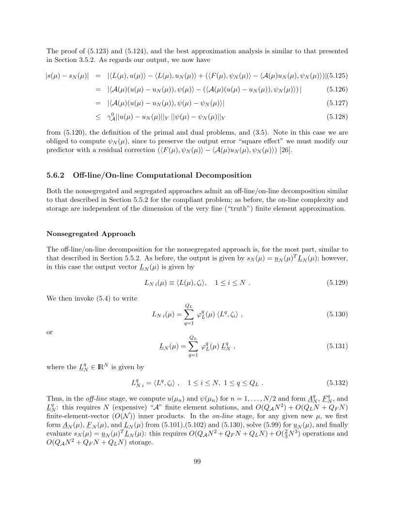
The proof of (5.123) and (5.124), and the best approximation analysis is similar to that presentedin Section 3.5.2. As regards our output, we now have

|s(µ)− sN (µ)| = |〈L(µ), u(µ)〉 − 〈L(µ), uN (µ)〉+ (〈F (µ), ψN (µ)〉 − 〈A(µ)uN (µ), ψN (µ)〉)|(5.125)

= |〈A(µ)(u(µ)− uN (µ)), ψ(µ)〉 − (〈A(µ)(u(µ)− uN (µ)), ψN (µ)〉) | (5.126)

= |〈A(µ)(u(µ)− uN (µ)), ψ(µ)− ψN (µ)〉| (5.127)

≤ γ0A||u(µ)− uN (µ)||Y ||ψ(µ)− ψN (µ)||Y (5.128)

from (5.120), the definition of the primal and dual problems, and (3.5). Note in this case we areobliged to compute ψN (µ), since to preserve the output error “square effect” we must modify ourpredictor with a residual correction (〈F (µ), ψN (µ)〉 − 〈A(µ)uN (µ), ψN (µ)〉) [26].

5.6.2 Off-line/On-line Computational Decomposition

Both the nonsegregated and segregated approaches admit an off-line/on-line decomposition similarto that described in Section 5.5.2 for the compliant problem; as before, the on-line complexity andstorage are independent of the dimension of the very fine (“truth”) finite element approximation.

Nonsegregated Approach

The off-line/on-line decomposition for the nonsegregated approach is, for the most part, similar tothat described in Section 5.5.2. As before, the output is given by sN (µ) = uN (µ)TLN (µ); however,in this case the output vector LN (µ) is given by

LN i(µ) ≡ 〈L(µ), ζi〉, 1 ≤ i ≤ N . (5.129)

We then invoke (5.4) to write

LN i(µ) =QL∑q=1

ϕqL(µ) 〈Lq, ζi〉 , (5.130)

or

LN (µ) =QL∑q=1

ϕqL(µ) Lq

N , (5.131)

where the LqN ∈ IRN is given by

LqN i = 〈Lq, ζi〉 , 1 ≤ i ≤ N, 1 ≤ q ≤ QL . (5.132)

Thus, in the off-line stage, we compute u(µn) and ψ(µn) for n = 1, . . . , N/2 and form AqN , F q

N , andLq

N : this requires N (expensive) “A” finite element solutions, and O(QAN2) + O(QLN + QFN)finite-element-vector (O(N )) inner products. In the on-line stage, for any given new µ, we firstform AN (µ), FN (µ), and LN (µ) from (5.101),(5.102) and (5.130), solve (5.99) for uN (µ), and finallyevaluate sN (µ) = uN (µ)TLN (µ): this requires O(QAN2 +QFN +QLN) +O(2

3N3) operations and

O(QAN2 +QFN +QLN) storage.

99

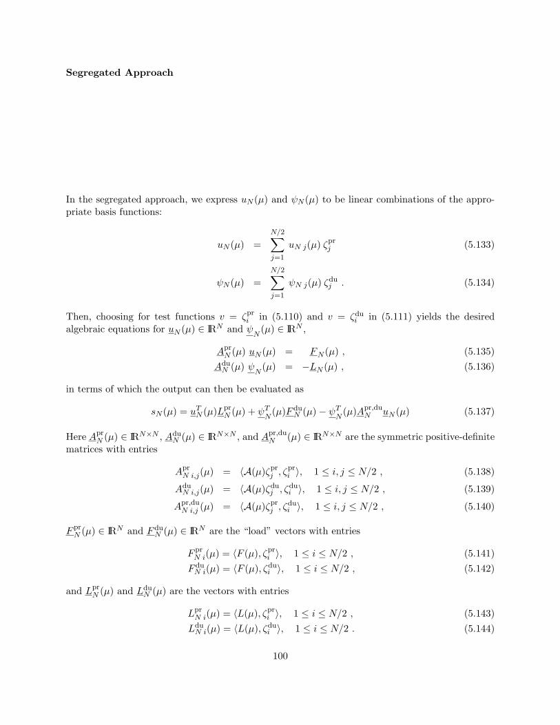
Segregated Approach

In the segregated approach, we express uN (µ) and ψN (µ) to be linear combinations of the appro-priate basis functions:

uN (µ) =N/2∑j=1

uN j(µ) ζprj (5.133)

ψN (µ) =N/2∑j=1

ψN j(µ) ζduj . (5.134)

Then, choosing for test functions v = ζpri in (5.110) and v = ζdu

i in (5.111) yields the desiredalgebraic equations for uN (µ) ∈ IRN and ψ

N(µ) ∈ IRN ,

AprN (µ) uN (µ) = FN (µ) , (5.135)

AduN (µ) ψ

N(µ) = −LN (µ) , (5.136)

in terms of which the output can then be evaluated as

sN (µ) = uTN (µ)Lpr

N (µ) + ψTN

(µ)F duN (µ)− ψT

N(µ)Apr,du

N uN (µ) (5.137)

Here AprN (µ) ∈ IRN×N , Adu

N (µ) ∈ IRN×N , and Apr,duN (µ) ∈ IRN×N are the symmetric positive-definite

matrices with entries

AprN i,j(µ) = 〈A(µ)ζpr

j , ζpri 〉, 1 ≤ i, j ≤ N/2 , (5.138)

AduN i,j(µ) = 〈A(µ)ζdu

j , ζdui 〉, 1 ≤ i, j ≤ N/2 , (5.139)

Apr,duN i,j (µ) = 〈A(µ)ζpr

j , ζdui 〉, 1 ≤ i, j ≤ N/2 , (5.140)

F prN (µ) ∈ IRN and F du

N (µ) ∈ IRN are the “load” vectors with entries

F prN i(µ) = 〈F (µ), ζpr

i 〉, 1 ≤ i ≤ N/2 , (5.141)F du

N i(µ) = 〈F (µ), ζdui 〉, 1 ≤ i ≤ N/2 , (5.142)

and LprN (µ) and Ldu

N (µ) are the vectors with entries

LprN i(µ) = 〈L(µ), ζpr

i 〉, 1 ≤ i ≤ N/2 , (5.143)Ldu

N i(µ) = 〈L(µ), ζdui 〉, 1 ≤ i ≤ N/2 . (5.144)

100

We again invoke (5.1)-(5.4) to write

AprN i,j(µ) =

QA∑q=1

Θq(µ) 〈Aqζprj , ζ

pri 〉 , (5.145)

AduN i,j(µ) =

QA∑q=1

Θq(µ) 〈Aqζduj , ζdu

i 〉 , (5.146)

Apr,duN i,j (µ) =

QA∑q=1

Θq(µ) 〈Aqζprj , ζ

dui 〉 , (5.147)

F prN i(µ) =

QF∑q=1

ϕqF (µ) 〈F q, ζpr

i 〉 , (5.148)

F duN i(µ) =

QF∑q=1

ϕqF (µ) 〈F q, ζdu

i 〉 , (5.149)

LprN i(µ) =

QL∑q=1

ϕqL(µ) 〈Lq, ζpr

i 〉 , (5.150)

LduN i(µ) =

QL∑q=1

ϕqL(µ) 〈Lq, ζdu

i 〉 , (5.151)

101

or

AprN (µ) =

QA∑q=1

Θq(µ)Aq prN , (5.152)

AduN (µ) =

QA∑q=1

Θq(µ)Aq duN , (5.153)

Apr,duN (µ) =

QA∑q=1

Θq(µ)Aq pr,duN , (5.154)

F prN (µ) =

QF∑q=1

ϕqF (µ) F q pr

N , (5.155)

F duN (µ) =

QF∑q=1

ϕqF (µ) F q du

N , (5.156)

LprN (µ) =

QL∑q=1

ϕqL(µ) Lq pr

N , (5.157)

LduN (µ) =

QL∑q=1

ϕqL(µ) Lq du

N , (5.158)

where the Aq prN , Aq du

N , Aq pr,duN , F q pr

N , F q duN , Lq pr

N and Lq duN are given by

Aq prN i,j = 〈Aqζpr

j , ζpri 〉 , 1 ≤ i, j ≤ N/2 1 ≤ q ≤ QA , (5.159)

Aq duN i,j = 〈Aqζdu

j , ζdui 〉 , 1 ≤ i, j ≤ N/2 1 ≤ q ≤ QA , (5.160)

Aq pr,duN i,j = 〈Aqζpr

j , ζdui 〉 , 1 ≤ i, j ≤ N/2 1 ≤ q ≤ QA , (5.161)

F q prN i = 〈F q, ζpr

i 〉 , 1 ≤ i ≤ N/2 1 ≤ q ≤ QF , (5.162)

F q duN i = 〈F q, ζdu

i 〉 , 1 ≤ i ≤ N/2 1 ≤ q ≤ QF , (5.163)Lq pr

N i = 〈Lq, ζpri 〉 , 1 ≤ i ≤ N/2 1 ≤ q ≤ QL , (5.164)

Lq duN i = 〈Lq, ζdu

i 〉 , 1 ≤ i ≤ N/2 1 ≤ q ≤ QL . (5.165)

Thus, in the off-line stage, we compute the u(µn), ψ(µn), and form the Aq prN , Aq du

N , Aq pr,duN , F q pr

N ,F q du

N , Lq prN , and Lq du

N : this requires N (expensive) “A” finite element solutions, and O(34QN

2) +O(QFN +QLN) finite-element-vector (O(N )) inner products. In the on-line stage, for any givennew µ, we first form Apr

N (µ), AduN (µ), Apr,du

N (µ), F prN (µ), F du

N (µ), LprN (µ), and Ldu

N (µ) from (5.152)-(5.158), then solve (5.135) and (5.136) for uN (µ) and ψ

N(µ), respectively, and finally evaluate

sN (µ): this requires O(34QAN

2+QFN+QLN)+O(43N

3) operations and O(34QAN

2+QFN+QLN)storage.

102

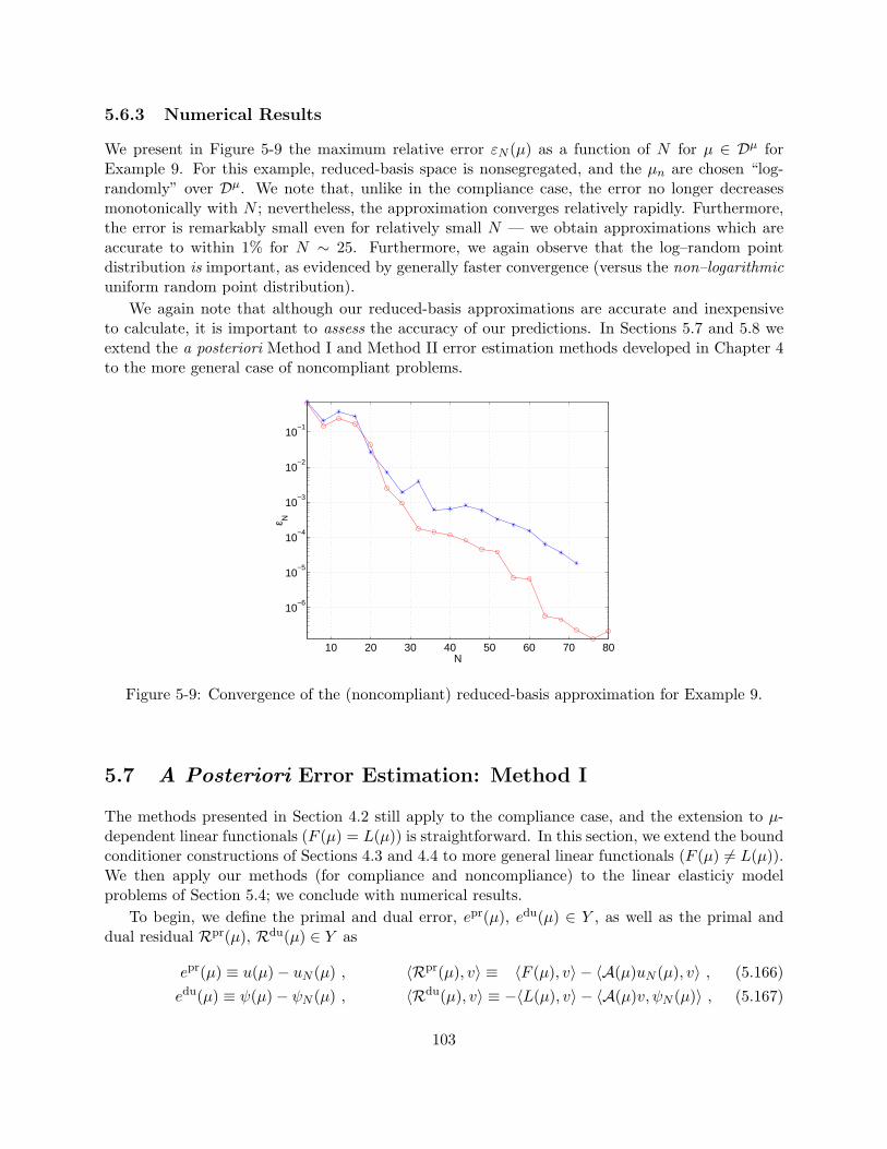
5.6.3 Numerical Results

We present in Figure 5-9 the maximum relative error εN (µ) as a function of N for µ ∈ Dµ forExample 9. For this example, reduced-basis space is nonsegregated, and the µn are chosen “log-randomly” over Dµ. We note that, unlike in the compliance case, the error no longer decreasesmonotonically with N ; nevertheless, the approximation converges relatively rapidly. Furthermore,the error is remarkably small even for relatively small N — we obtain approximations which areaccurate to within 1% for N ∼ 25. Furthermore, we again observe that the log–random pointdistribution is important, as evidenced by generally faster convergence (versus the non–logarithmicuniform random point distribution).

We again note that although our reduced-basis approximations are accurate and inexpensiveto calculate, it is important to assess the accuracy of our predictions. In Sections 5.7 and 5.8 weextend the a posteriori Method I and Method II error estimation methods developed in Chapter 4to the more general case of noncompliant problems.

10 20 30 40 50 60 70 80

10−6

10−5

10−4

10−3

10−2

10−1

N

ε N

Figure 5-9: Convergence of the (noncompliant) reduced-basis approximation for Example 9.

5.7 A Posteriori Error Estimation: Method I

The methods presented in Section 4.2 still apply to the compliance case, and the extension to µ-dependent linear functionals (F (µ) = L(µ)) is straightforward. In this section, we extend the boundconditioner constructions of Sections 4.3 and 4.4 to more general linear functionals (F (µ) 6= L(µ)).We then apply our methods (for compliance and noncompliance) to the linear elasticiy modelproblems of Section 5.4; we conclude with numerical results.

To begin, we define the primal and dual error, epr(µ), edu(µ) ∈ Y , as well as the primal anddual residual Rpr(µ), Rdu(µ) ∈ Y as

epr(µ) ≡ u(µ)− uN (µ) , 〈Rpr(µ), v〉 ≡ 〈F (µ), v〉 − 〈A(µ)uN (µ), v〉 , (5.166)edu(µ) ≡ ψ(µ)− ψN (µ) , 〈Rdu(µ), v〉 ≡ −〈L(µ), v〉 − 〈A(µ)v, ψN (µ)〉 , (5.167)

103

from which it follows that

〈A(µ)epr(µ), v〉 = 〈Rpr(µ), v〉 , (5.168)〈A(µ)v, edu(µ)〉 = 〈Rdu(µ), v〉 . (5.169)

5.7.1 Bound Conditioner

We again introduce a symmetric, continuous, and coercive bound conditioner [21, 37, 47] C(µ) : Y →Y ′ such that the eigenvalues

ρmin(µ) = minv∈Y

〈A(µ)v, v〉〈C(µ)v, v〉

, (5.170)

ρmax(µ) = maxv∈Y

〈A(µ)v, v〉〈C(µ)v, v〉

, (5.171)

satisfy1 ≤ ρmin(µ), ρmax(µ) ≤ ρ, (5.172)

for some (preferably small) constant ρ ∈ IR. As before, we also require an additional “computationalinvertibility” hypothesis [38, 47]: we require that C−1(µ) be of the form

C−1(µ) =∑

i∈I(µ)

αi(µ)C−1i (5.173)

where I(µ) ⊂ 1, . . . , I is a parameter-dependent set of indices, I is a finite (preferably small)integer, and the Ci : Y → Y ′, i = 1, . . . , I, are parameter-independent symmetric, coercive operators.

5.7.2 Error and Output Bounds

We now find epr(µ) ∈ Y and edu(µ) ∈ Y such that

〈C(µ)epr(µ), v〉 = 〈Rpr(µ), v〉, ∀ v ∈ Y , (5.174)〈C(µ)edu(µ), v〉 = 〈Rdu(µ), v〉, ∀ v ∈ Y . (5.175)

We then define our lower and upper output bounds as

s−N (µ) = sN (µ)−∆N (µ) (5.176)s+N (µ) = sN (µ) + ∆N (µ) (5.177)

where ∆N (µ) is given by

∆N (µ) = 〈C(µ)epr(µ), epr(µ)〉1/2〈C(µ)edu(µ), edu(µ)〉1/2 (5.178)= 〈Rpr(µ), C−1(µ)Rpr(µ)〉1/2〈Rdu(µ), C−1(µ)Rdu(µ)〉1/2 (5.179)= 〈Rpr(µ), epr(µ)〉1/2〈Rdu(µ), edu(µ)〉1/2 . (5.180)

104

5.7.3 Bounding Properties

It remains to demonstrate that

ηN (µ) =∆N (µ)

|s(µ)− sN (µ)|≥ 1 , ∀ N ≥ 1 , (5.181)

and to investigate the sharpness of our bounds; note that from (5.176), (5.177), and (5.181) itdirectly follows that that s−N (µ) ≤ s(µ) ≤ s+N (µ) for all N ≥ 1.

To prove (5.181), we first note from (5.117) for the nonsegregated case, and (5.127) for thesegregated case, that

|s(µ)− sN (µ)| = |〈A(µ)epr(µ), edu(µ)〉|. (5.182)

It then follows that

ηN (µ) =〈C(µ)epr(µ), epr(µ)〉1/2〈C(µ)edu(µ), edu(µ)〉1/2

|〈A(µ)epr(µ), edu(µ)〉|(5.183)

≥ 〈C(µ)epr(µ), epr(µ)〉1/2〈C(µ)edu(µ), edu(µ)〉1/2

〈A(µ)epr(µ), epr(µ)〉1/2〈A(µ)edu(µ), edu(µ)〉1/2(5.184)

≥ ρmin(µ) (5.185)≥ 1 , (5.186)

from the triangle inequality and (4.21).

We now turn to the upper effectivity inequality (sharpness property). We note from (5.183) thatif the primal and dual errors are A-orthogonal, or become increasingly orthogonal as N increases,such that |〈A(µ)epr(µ), edu(µ)〉| → 0, then the effectivity will not be bounded as N →∞. However,if we make the (plausible) hypothesis [39] that

|s(µ)− sN (µ)| =∣∣∣〈A(µ)epr(µ), edu(µ)〉

∣∣∣ ≥ c 0A||epr(µ)||Y ||edu(µ)||Y , (5.187)

then it follows that

ηN (µ) =〈C(µ)epr(µ), epr(µ)〉1/2〈C(µ)edu(µ), edu(µ)〉1/2

|〈A(µ)epr(µ), edu(µ)〉|(5.188)

≤ 〈C(µ)epr(µ), epr(µ)〉1/2〈C(µ)edu(µ), edu(µ)〉1/2

c 0A||epr(µ)||Y ||edu(µ)||Y

(5.189)

≤γ0Ac 0A

〈C(µ)epr(µ), epr(µ)〉1/2〈C(µ)edu(µ), edu(µ)〉1/2

〈A(µ)epr(µ), epr(µ)〉1/2〈A(µ)edu(µ), edu(µ)〉1/2(5.190)

≤γ0Ac 0Aρmax(µ) (5.191)

≤γ0Ac 0Aρ . (5.192)

105

5.7.4 Off-line/On-line Computational Procedure

We indicate here the off-line/on-line calculation of ∆N (µ) for the nonsegregated cases; the segre-gated approach admit a similar computational decomposition.

Nonsegregated Case

We recall from (5.179) that

∆N (µ) = 〈Rpr(µ), C−1(µ)Rpr(µ)〉1/2〈Rdu(µ), C−1(µ)Rdu(µ)〉1/2 . (5.193)

From the definition of the residual (5.166)-(5.167), the separability assumption (5.1), and theexpansion of uN (µ) and ψN (µ) in terms of the basis functions, we have

〈Rpr(µ), v〉 = 〈F (µ), v〉 − 〈A(µ)uN (µ), v〉

=QF∑q=1

ϕqF (µ)〈F q, v〉 −

QA∑q=1

N∑n=1

Θq(µ) uN n(µ) 〈Aqζn, v〉, ∀ v ∈ Y, ∀ µ ∈ Dµ ,

and

〈Rdu(µ), v〉 = −〈L(µ), v〉 − 〈A(µ)ψN (µ), v〉

= −QL∑q=1

ϕqL(µ)〈Lq, v〉 −

QA∑q=1

N∑n=1

Θq(µ) ψN n(µ) 〈Aqζn, v〉, ∀ v ∈ Y, ∀ µ ∈ Dµ .

We now invoke the “computational invertibility” hypothesis on C(µ), (5.173), to write

〈Rpr(µ), C−1(µ)Rpr(µ)〉 =∑

i∈I(µ)

αi(µ) 〈Rpr(µ), C−1i Rpr(µ)〉 (5.194)

=∑

i∈I(µ)

αi(µ)

⟨QF∑q=1

ϕqF (µ)F q −

QA∑q=1

N∑n=1

Θq(µ) uN n(µ)Aqζn,

C−1i

QF∑q′=1

ϕq′

F (µ)F q′ −QA∑q′=1

N∑n′=1

Θq′(µ) uN n′(µ)Aq′ζn′

⟩

=∑

i∈I(µ)

αi(µ)

QF∑q=1

QF∑q′=1

ϕqF (µ)ϕq′

F (µ)〈F q, C−1i F q′〉

−QA∑q=1

QF∑q′=1

N∑n=1

Θq(µ) ϕq′

F (µ) uN n(µ)(〈F q′ , C−1

i Aqζn〉+ 〈Aqζn, C−1i F q′〉

)

+QA∑q=1

QA∑q′=1

N∑n=1

N∑n′=1

Θq(µ) Θq′(µ) uN n(µ) uN n′(µ) 〈Aqζn, C−1i Aq′ζn′〉

;

106

similarly, we have

〈Rdu(µ), C−1(µ)Rdu(µ)〉 =∑

i∈I(µ)

αi(µ)

QL∑q=1

QL∑q′=1

ϕqL(µ)ϕq′

L (µ)〈Lq, C−1i Lq′〉

+QA∑q=1

QL∑q′=1

N∑n=1

Θq(µ) ϕq′

L (µ) ψN n(µ)(〈Lq′ , C−1

i Aqζn〉+ 〈Aqζn, C−1i Lq′〉

)

+QA∑q=1

QA∑q′=1

N∑n=1

N∑n′=1

Θq(µ) Θq′(µ) ψN n(µ) ψN n′(µ) 〈Aqζn, C−1i Aq′ζn′〉

.Thus, in the off-line stage, we compute the µ-independent inner products

cpriqq′ = 〈F q, C−1

i F q′〉 , 1 ≤ i ≤ I, 1 ≤ q, q′ ≤ QF (5.195)

cduiqq′ = 〈Lq, C−1

i Lq′〉 , 1 ≤ i ≤ I, 1 ≤ q, q′ ≤ QL (5.196)

Λpriqq′n = −〈F q′ , C−1

i Aqζn〉 = −〈Aqζn, C−1i F q′〉 , 1 ≤ i ≤ I, 1 ≤ q ≤ QA, (5.197)

1 ≤ q′ ≤ QF , 1 ≤ n ≤ N, (5.198)Λdu

iqq′n = 〈Lq′ , C−1i Aqζn〉 = 〈Aqζn, C−1

i Lq′〉 , 1 ≤ i ≤ I, 1 ≤ q ≤ QA, (5.199)1 ≤ q′ ≤ QL, 1 ≤ n ≤ N, (5.200)

and

Γqq′nn′ = 〈Aqζn, C−1i Aq′ζn′〉 , 1 ≤ q, q′ ≤ QA, 1 ≤ n, n′ ≤ N, (5.201)

where (5.197) and (5.199) follow from the symmetry of Ci. Calculation of (5.195)-(5.201) thenrequires QAN Aqζn multiplications, I(QAN+QF +QL) C-solves, and I(Q2

AN2+QAN+QFQAN+

QLQAN +Q2F +Q2

L) inner products.

In the on-line stage, given any new value of µ, we simply the compute

∆N (µ) =

∑i∈I(µ)

αi(µ)

QF∑q=1

QF∑q′=1

ϕqF (µ)ϕq′

F (µ)cpriqq′ + 2

QA∑q=1

QF∑q′=1

N∑n=1

Θq(µ) ϕq′

F (µ) uN n(µ) Λpriqq′n

+QA∑q=1

QA∑q′=1

N∑n=1

N∑n′=1

Θq(µ) Θq′(µ) uN n(µ) uN n′(µ) Γqq′nn′

1/2

(5.202)

∑i∈I(µ)

αi(µ)

QL∑q=1

QL∑q′=1

ϕqL(µ)ϕq′

L (µ)cduiqq′ + 2

QA∑q=1

QL∑q′=1

N∑n=1

Θq(µ) ϕq′

L (µ) ψN n(µ) Λduiqq′n

+QA∑q=1

QA∑q′=1

N∑n=1

N∑n′=1

Θq(µ) Θq′(µ) ψN n(µ) ψN n′(µ) Γqq′nn′

1/2

. (5.203)

The on-line complexity is thus, to leading order, O(|I(µ)|Q2AN

2) — and hence, independent of N .

107

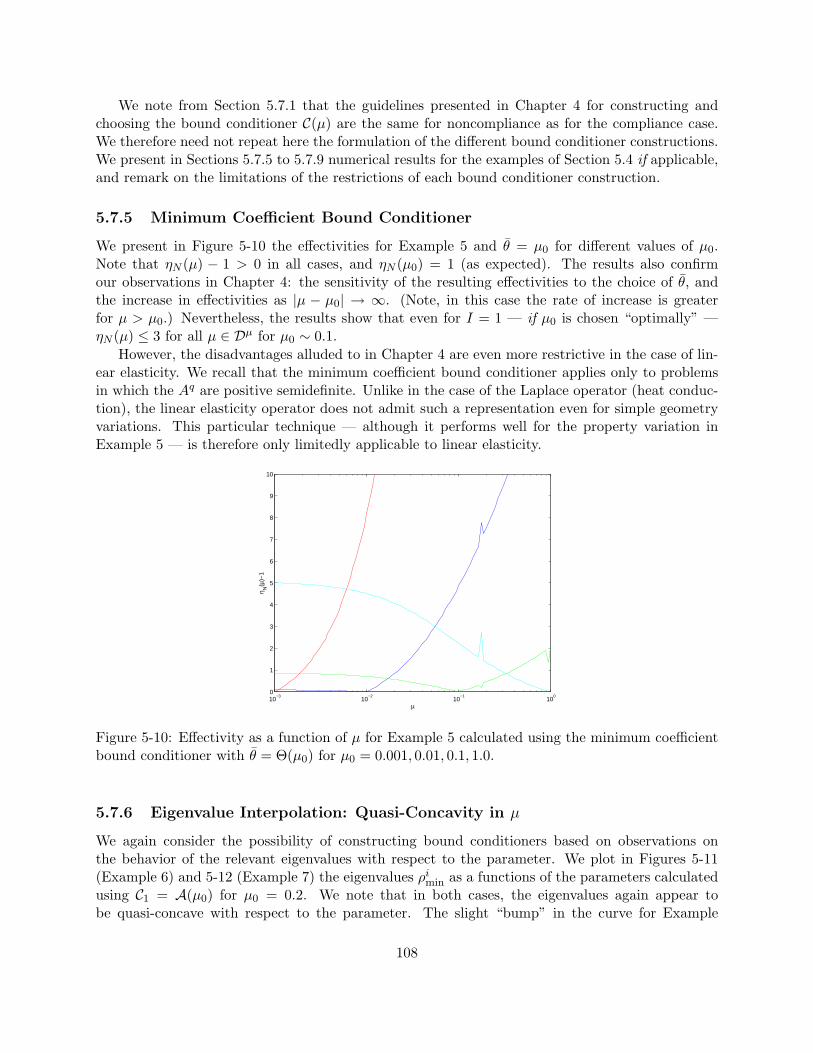
We note from Section 5.7.1 that the guidelines presented in Chapter 4 for constructing andchoosing the bound conditioner C(µ) are the same for noncompliance as for the compliance case.We therefore need not repeat here the formulation of the different bound conditioner constructions.We present in Sections 5.7.5 to 5.7.9 numerical results for the examples of Section 5.4 if applicable,and remark on the limitations of the restrictions of each bound conditioner construction.

5.7.5 Minimum Coefficient Bound Conditioner

We present in Figure 5-10 the effectivities for Example 5 and θ = µ0 for different values of µ0.Note that ηN (µ) − 1 > 0 in all cases, and ηN (µ0) = 1 (as expected). The results also confirmour observations in Chapter 4: the sensitivity of the resulting effectivities to the choice of θ, andthe increase in effectivities as |µ − µ0| → ∞. (Note, in this case the rate of increase is greaterfor µ > µ0.) Nevertheless, the results show that even for I = 1 — if µ0 is chosen “optimally” —ηN (µ) ≤ 3 for all µ ∈ Dµ for µ0 ∼ 0.1.

However, the disadvantages alluded to in Chapter 4 are even more restrictive in the case of lin-ear elasticity. We recall that the minimum coefficient bound conditioner applies only to problemsin which the Aq are positive semidefinite. Unlike in the case of the Laplace operator (heat conduc-tion), the linear elasticity operator does not admit such a representation even for simple geometryvariations. This particular technique — although it performs well for the property variation inExample 5 — is therefore only limitedly applicable to linear elasticity.

10−3

10−2

10−1

100

0

1

2

3

4

5

6

7

8

9

10

µ

η N(µ

)−1

Figure 5-10: Effectivity as a function of µ for Example 5 calculated using the minimum coefficientbound conditioner with θ = Θ(µ0) for µ0 = 0.001, 0.01, 0.1, 1.0.

5.7.6 Eigenvalue Interpolation: Quasi-Concavity in µ

We again consider the possibility of constructing bound conditioners based on observations onthe behavior of the relevant eigenvalues with respect to the parameter. We plot in Figures 5-11(Example 6) and 5-12 (Example 7) the eigenvalues ρi

min as a functions of the parameters calculatedusing C1 = A(µ0) for µ0 = 0.2. We note that in both cases, the eigenvalues again appear tobe quasi-concave with respect to the parameter. The slight “bump” in the curve for Example

108

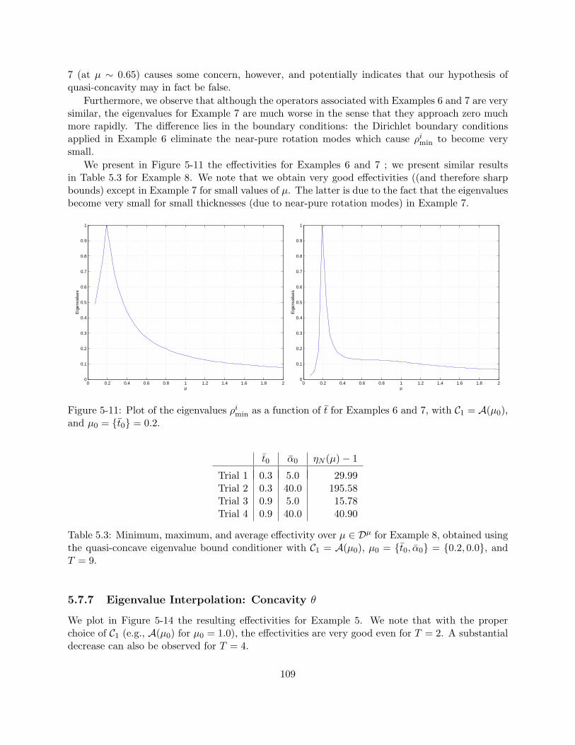
7 (at µ ∼ 0.65) causes some concern, however, and potentially indicates that our hypothesis ofquasi-concavity may in fact be false.

Furthermore, we observe that although the operators associated with Examples 6 and 7 are verysimilar, the eigenvalues for Example 7 are much worse in the sense that they approach zero muchmore rapidly. The difference lies in the boundary conditions: the Dirichlet boundary conditionsapplied in Example 6 eliminate the near-pure rotation modes which cause ρi

min to become verysmall.

We present in Figure 5-11 the effectivities for Examples 6 and 7 ; we present similar resultsin Table 5.3 for Example 8. We note that we obtain very good effectivities ((and therefore sharpbounds) except in Example 7 for small values of µ. The latter is due to the fact that the eigenvaluesbecome very small for small thicknesses (due to near-pure rotation modes) in Example 7.

0 0.2 0.4 0.6 0.8 1 1.2 1.4 1.6 1.8 20

0.1

0.2

0.3

0.4

0.5

0.6

0.7

0.8

0.9

1

µ

Eig

enva

lues

0 0.2 0.4 0.6 0.8 1 1.2 1.4 1.6 1.8 20

0.1

0.2

0.3

0.4

0.5

0.6

0.7

0.8

0.9

1

µ

Eig

enva

lues

Figure 5-11: Plot of the eigenvalues ρimin as a function of t for Examples 6 and 7, with C1 = A(µ0),

and µ0 = t0 = 0.2.

t0 α0 ηN (µ)− 1

Trial 1 0.3 5.0 29.99Trial 2 0.3 40.0 195.58Trial 3 0.9 5.0 15.78Trial 4 0.9 40.0 40.90

Table 5.3: Minimum, maximum, and average effectivity over µ ∈ Dµ for Example 8, obtained usingthe quasi-concave eigenvalue bound conditioner with C1 = A(µ0), µ0 = t0, α0 = 0.2, 0.0, andT = 9.

5.7.7 Eigenvalue Interpolation: Concavity θ

We plot in Figure 5-14 the resulting effectivities for Example 5. We note that with the properchoice of C1 (e.g., A(µ0) for µ0 = 1.0), the effectivities are very good even for T = 2. A substantialdecrease can also be observed for T = 4.

109

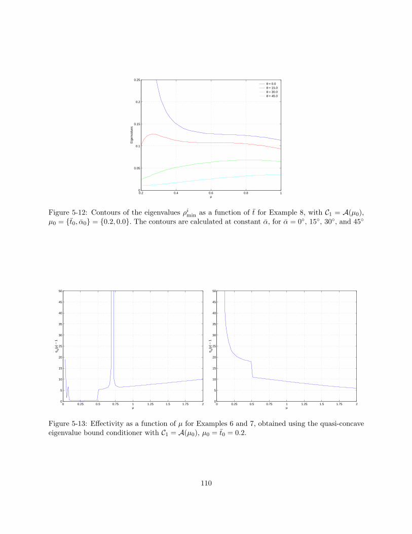
0.2 0.4 0.6 0.8 10

0.05

0.1

0.15

0.2

0.25

µ

Eig

enva

lues

θ = 0.0θ = 15.0θ = 30.0θ = 45.0

Figure 5-12: Contours of the eigenvalues ρimin as a function of t for Example 8, with C1 = A(µ0),

µ0 = t0, α0 = 0.2, 0.0. The contours are calculated at constant α, for α = 0, 15, 30, and 45

0 0.25 0.5 0.75 1 1.25 1.5 1.75 20

5

10

15

20

25

30

35

40

45

50

µ

η N(µ

) −

1

0 0.25 0.5 0.75 1 1.25 1.5 1.75 20

5

10

15

20

25

30

35

40

45

50

µ

η N(µ

) −

1

Figure 5-13: Effectivity as a function of µ for Examples 6 and 7, obtained using the quasi-concaveeigenvalue bound conditioner with C1 = A(µ0), µ0 = t0 = 0.2.

110

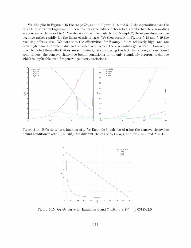
We also plot in Figure 5-15 the range Dθ, and in Figures 5-16 and 5-12 the eigenvalues over thethree lines shown in Figure 5-15. These results agree with our theoretical results that the eigenvaluesare concave with respect to θ. We also note that, particularly for Example 7, the eigenvalues becomenegative rather rapidly for the linear elasticity case. We then present in Figures 5-18 and 5-19 theresulting effectivities. We note that the effectivities for Example 6 are relatively high, and areeven higher for Example 7 due to the speed with which the eigenvalues go to zero. However, itmust be noted these effectivities are still quite good considering the fact that among all our boundconditioners, the concave eigenvalue bound conditioner is the only completely rigorous techniquewhich is applicable even for general geometry variations.

10−3

10−2

10−1

100

0

10

20

30

40

50

60

70

80

90

100

µ

η N(µ

)−1

µ0 = 0.001

µ0 = 0.01

µ0 = 0.1

µ0 = 1.0

10−3

10−2

10−1

100

0

10

20

30

40

50

60

70

80

90

100

µ

η N(µ

)−1

µ0 = 0.001

µ0 = 0.01

µ0 = 0.1

µ0 = 1.0

Figure 5-14: Effectivity as a function of µ for Example 5, calculated using the concave eigenvaluebound conditioner with C1 = A(θ0) for different choices of θ0 (= µ0), and for T = 2 and T = 4.

0 0.2 0.4 0.6 0.8 1 1.2 1.4 1.6 1.8 20

5

10

15

20

25

30

35

θ1

θ 2

Θ1−Θ

2 curve

Line 1Line 2Line 3

Figure 5-15: Θ1-Θ2 curve for Examples 6 and 7, with µ ∈ Dµ = [0.03125, 2.0].

111

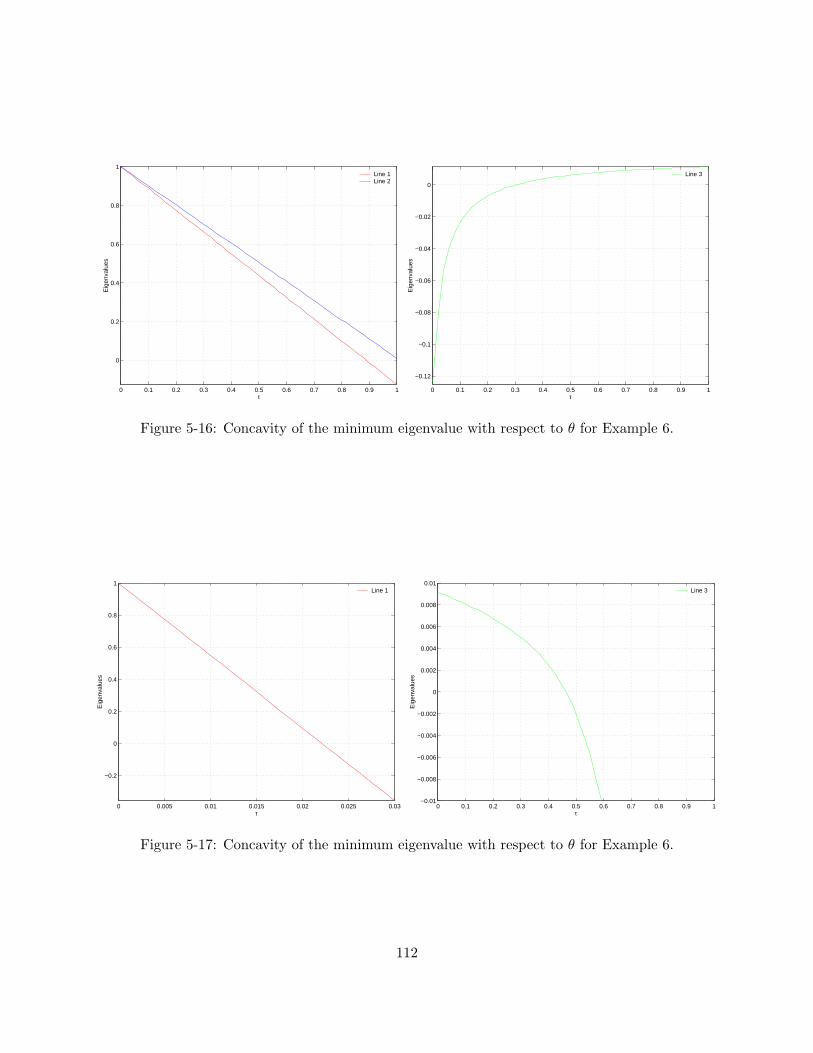
0 0.1 0.2 0.3 0.4 0.5 0.6 0.7 0.8 0.9 1

0

0.2

0.4

0.6

0.8

1

τ

Eig

enva

lues

Line 1Line 2

0 0.1 0.2 0.3 0.4 0.5 0.6 0.7 0.8 0.9 1

−0.12

−0.1

−0.08

−0.06

−0.04

−0.02

0

τ

Eig

enva

lues

Line 3

Figure 5-16: Concavity of the minimum eigenvalue with respect to θ for Example 6.

0 0.005 0.01 0.015 0.02 0.025 0.03

−0.2

0

0.2

0.4

0.6

0.8

1

τ

Eig

enva

lues

Line 1

0 0.1 0.2 0.3 0.4 0.5 0.6 0.7 0.8 0.9 1−0.01

−0.008

−0.006

−0.004

−0.002

0

0.002

0.004

0.006

0.008

0.01

τ

Eig

enva

lues

Line 3

Figure 5-17: Concavity of the minimum eigenvalue with respect to θ for Example 6.

112

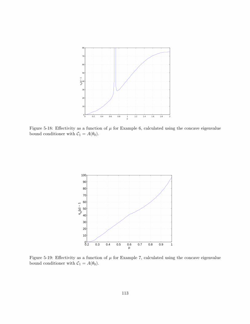
0 0.2 0.4 0.6 0.8 1 1.2 1.4 1.6 1.8 20

10

20

30

40

50

60

70

80

µ

η N(µ

) −

1

Figure 5-18: Effectivity as a function of µ for Example 6, calculated using the concave eigenvaluebound conditioner with C1 = A(θ0).

0.2 0.3 0.4 0.5 0.6 0.7 0.8 0.9 10

10

20

30

40

50

60

70

80

90

100

µ

η N(µ

) −

1

Figure 5-19: Effectivity as a function of µ for Example 7, calculated using the concave eigenvaluebound conditioner with C1 = A(θ0).

113

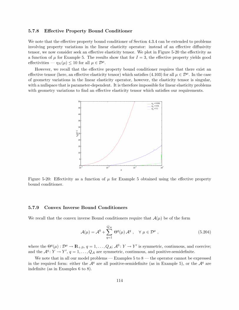
5.7.8 Effective Property Bound Conditioner

We note that the effective property bound conditioner of Section 4.3.4 can be extended to problemsinvolving property variations in the linear elasticity operator: instead of an effective diffusivitytensor, we now consider seek an effective elasticity tensor. We plot in Figure 5-20 the effectivity asa function of µ for Example 5. The results show that for I = 3, the effective property yields goodeffectivities — ηN (µ) ≤ 10 for all µ ∈ Dµ.

However, we recall that the effective property bound conditioner requires that there exist aneffective tensor (here, an effective elasticity tensor) which satisfies (4.103) for all µ ∈ Dµ. In the caseof geometry variations in the linear elasticity operator, however, the elasticity tensor is singular,with a nullspace that is parameter-dependent. It is therefore impossible for linear elasticity problemswith geometry variations to find an effective elasticity tensor which satisfies our requirements.

10−3

10−2

10−1

100

0

5

10

15

20

25

30

35

40

45

50

µ

η N(µ

)−1

µ0 = 0.001

µ0 = 0.01

µ0 = 0.1

Figure 5-20: Effectivity as a function of µ for Example 5 obtained using the effective propertybound conditioner.

5.7.9 Convex Inverse Bound Conditioners

We recall that the convex inverse Bound conditioners require that A(µ) be of the form

A(µ) = A0 +QA∑q=1

Θq(µ)Aq , ∀ µ ∈ Dµ , (5.204)

where the Θq(µ) : Dµ → IR+,0, q = 1, . . . , QA; A0 : Y → Y ′ is symmetric, continuous, and coercive;and the Aq : Y → Y ′, q = 1, . . . , QA are symmetric, continuous, and positive-semidefinite.

We note that in all our model problems — Examples 5 to 8 — the operator cannot be expressedin the required form: either the Aq are all positive-semidefinite (as in Example 5), or the Aq areindefinite (as in Examples 6 to 8).

114

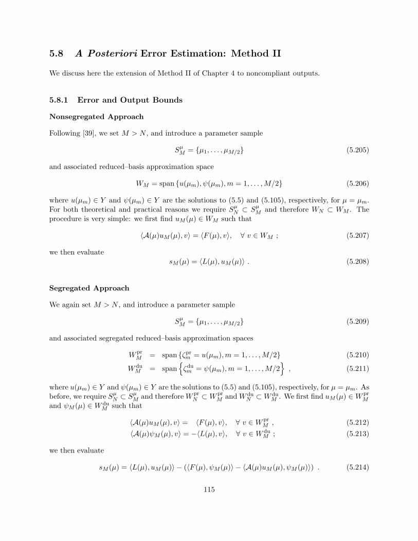
5.8 A Posteriori Error Estimation: Method II

We discuss here the extension of Method II of Chapter 4 to noncompliant outputs.

5.8.1 Error and Output Bounds

Nonsegregated Approach

Following [39], we set M > N , and introduce a parameter sample

SµM = µ1, . . . , µM/2 (5.205)

and associated reduced–basis approximation space

WM = span u(µm), ψ(µm),m = 1, . . . ,M/2 (5.206)

where u(µm) ∈ Y and ψ(µm) ∈ Y are the solutions to (5.5) and (5.105), respectively, for µ = µm.For both theoretical and practical reasons we require Sµ

N ⊂ SµM and therefore WN ⊂ WM . The

procedure is very simple: we first find uM (µ) ∈WM such that

〈A(µ)uM (µ), v〉 = 〈F (µ), v〉, ∀ v ∈WM ; (5.207)

we then evaluatesM (µ) = 〈L(µ), uM (µ)〉 . (5.208)

Segregated Approach

We again set M > N , and introduce a parameter sample

SµM = µ1, . . . , µM/2 (5.209)

and associated segregated reduced–basis approximation spaces

W prM = span ζpr

m = u(µm),m = 1, . . . ,M/2 (5.210)

W duM = span

ζdum = ψ(µm),m = 1, . . . ,M/2

, (5.211)

where u(µm) ∈ Y and ψ(µm) ∈ Y are the solutions to (5.5) and (5.105), respectively, for µ = µm. Asbefore, we require Sµ

N ⊂ SµM and therefore W pr

N ⊂W prM and W du

N ⊂W duM . We first find uM (µ) ∈W pr

M

and ψM (µ) ∈W duM such that

〈A(µ)uM (µ), v〉 = 〈F (µ), v〉, ∀ v ∈W prM , (5.212)

〈A(µ)ψM (µ), v〉 = −〈L(µ), v〉, ∀ v ∈W duM ; (5.213)

we then evaluate

sM (µ) = 〈L(µ), uM (µ)〉 − (〈F (µ), ψM (µ)〉 − 〈A(µ)uM (µ), ψM (µ)〉) . (5.214)

115

Output Bounds

Given sN (µ) and sM (µ) calculated using either the nonsegregated or segregated approaches, weevaluate the “improved” estimator sN (µ) given by

sN (µ) = sN (µ)− 12τ

(sM (µ)− sN (µ)) ; (5.215)

our lower and upper output bounds are then

s−N (µ) = sN (µ)− 12∆N (µ) (5.216)

s+N (µ) = sN (µ) +12∆N (µ) (5.217)

where ∆N (µ) is given by

∆N,M (µ) =1τ|sM (µ)− sN (µ)| (5.218)

for some τ ∈ (0, 1). The effectivity of the approximation is defined as

ηN,M (µ) =∆N,M (µ)

|s(µ)− sN (µ)|. (5.219)

We shall again only consider M = 2N .

5.8.2 Bounding Properties

As in Section 4.5, we would like to prove the effectivity inequality 1 ≤ ηN,2N (µ) ≤ ρ, for sufficientlylarge N ; as in Section 4.5, we must again make the hypothesis (4.190). We first consider the lowereffectivity inequality, ηN,M (µ) ≥ 1, and prove the equivalent statement

s−N,2N (µ) ≤ s(µ) ≤ s+N,2N (µ), N →∞. (5.220)

Following [39], we write

s−N,2N (µ) = s(µ)− 11− εN,2N

|sN (µ)− s2N (µ)|

×

1 s2N (µ) ≥ sN (µ)1τ (1− εN,2N )− 1 s2N (µ) < sN (µ) ,

(5.221)

s+N,2N (µ) = s(µ) +1

1− εN,2N|sN (µ)− s2N (µ)|

×

1τ (1− εN,2N )− 1 s2N (µ) ≥ sN (µ)1 s2N (µ) < sN (µ).

(5.222)

From our hypothesis on εN,2N , (4.190), and the range of τ , there exists an N∗ such that for N > N∗,1τ (1− εN,2N ) > 1; the result (5.220) directly follows.

We now consider the upper effectivity inequality (sharpness property). As in Section 4.5, we

116

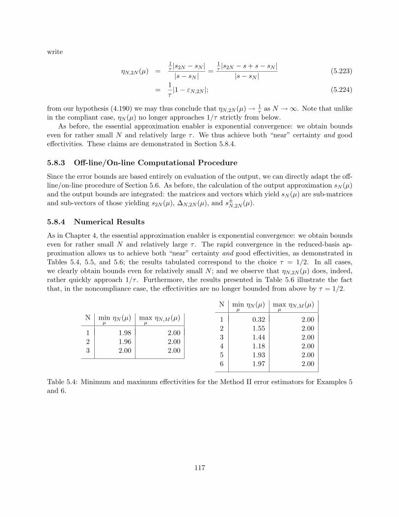
write

ηN,2N (µ) =1τ |s2N − sN ||s− sN |

=1τ |s2N − s+ s− sN |

|s− sN |(5.223)

=1τ|1− εN,2N |; (5.224)

from our hypothesis (4.190) we may thus conclude that ηN,2N (µ) → 1τ as N →∞. Note that unlike

in the compliant case, ηN (µ) no longer approaches 1/τ strictly from below.As before, the essential approximation enabler is exponential convergence: we obtain bounds

even for rather small N and relatively large τ . We thus achieve both “near” certainty and goodeffectivities. These claims are demonstrated in Section 5.8.4.

5.8.3 Off-line/On-line Computational Procedure

Since the error bounds are based entirely on evaluation of the output, we can directly adapt the off-line/on-line procedure of Section 5.6. As before, the calculation of the output approximation sN (µ)and the output bounds are integrated: the matrices and vectors which yield sN (µ) are sub-matricesand sub-vectors of those yielding s2N (µ), ∆N,2N (µ), and s±N,2N (µ).

5.8.4 Numerical Results

As in Chapter 4, the essential approximation enabler is exponential convergence: we obtain boundseven for rather small N and relatively large τ . The rapid convergence in the reduced-basis ap-proximation allows us to achieve both “near” certainty and good effectivities, as demonstrated inTables 5.4, 5.5, and 5.6; the results tabulated correspond to the choice τ = 1/2. In all cases,we clearly obtain bounds even for relatively small N ; and we observe that ηN,2N (µ) does, indeed,rather quickly approach 1/τ . Furthermore, the results presented in Table 5.6 illustrate the factthat, in the noncompliance case, the effectivities are no longer bounded from above by τ = 1/2.

N minµ

ηN (µ) maxµ

ηN,M (µ)

1 1.98 2.002 1.96 2.003 2.00 2.00

N minµ

ηN (µ) maxµ

ηN,M (µ)

1 0.32 2.002 1.55 2.003 1.44 2.004 1.18 2.005 1.93 2.006 1.97 2.00

Table 5.4: Minimum and maximum effectivities for the Method II error estimators for Examples 5and 6.

117

N minµ

ηN (µ) maxµ

ηN,M (µ)

1 0.18 1.992 0.92 1.993 1.55 2.004 1.56 2.005 1.96 2.006 1.92 2.007 1.78 2.00

N minµ

ηN (µ) maxµ

ηN,M (µ)

1 0.01 2.002 1.25 1.973 1.47 1.994 0.37 2.005 1.06 2.006 1.57 2.007 1.54 2.008 1.71 2.009 1.60 2.0010 1.70 2.00

Table 5.5: Minimum and maximum effectivities for the Method II error estimators for Examples 7and 8.

N minµ

ηN (µ) maxµ

ηN,M (µ)

4 0.30 3.608 0.16 2.0012 1.63 2.0116 1.43 2.0020 1.81 4.1524 1.54 2.0428 1.93 2.0132 1.96 2.0636 1.96 2.4440 1.97 2.00

Table 5.6: Minimum and maximum effectivities for the Method II error estimators for Example 9.

118

Chapter 6

Reduced-Basis Output Bounds forEigenvalue Problems: An ElasticStability Example

6.1 Introduction

There are many applications in which the posibility of unstable equilibria must be considered.Applied forces which exceed the critical loads may cause structures to buckle, resulting in large(and potentially dangerous) deformations; structural stability considerations must therefore beincluded in any design.

While analytical formulas exist for the critical loads of relatively simple geometries, they are oflimited applicability particularly for more complex structures. However, exact (finite element) solu-tion of the partial differential equations governing elastic stability is computationally too expensive,especially in the “many queries” context of design and optimization.

We consider here the reduced-basis approximation and (Method II) error estimation for theproblem of elastic buckling. The output of interest is the critical buckling load, calculation of whichrequires solution of a nonlinear (partial differential) eigenvalue problem. Note the nonlinearitypresents significant difficulties: the computational and storage requirements for the reduced-basisapproximation are greater, and our rigorous error estimation procedures are currently inapplicable.

6.2 Abstraction

As in Chapter 5, we consider a suitably regular (smooth) parameter-independent domain Ω ⊂IRd, d = 1, 2, or 3, the associated function space Y ⊂ (H1(Ω))d, with inner product (·, ·)Y , norm|| · ||Y = (·, ·)1/2

Y , dual space Y ′, and duality pairing 〈 ·, ·〉 = Y ′〈 ·, ·〉Y ; as before, we define aparameter set Dµ ∈ IRP , a particular point in which will be denoted µ.

We now introduce a symmetric, continuous, and coercive distributional operator A(µ) : Y → Y ′;a symmetric, continuous, and semi-definite distributional operator B(µ;w) : Y → Y ′; and boundedlinear form F (µ) ∈ Y ′. We shall again make certain assumptions on the parametric dependence ofA, B, and F . In particular, we shall suppose that, for some finite (preferably small) integers QA,

119

QB, and QF , we may express A(µ), B(µ), and F (µ) for all µ ∈ Dµ as

A(µ) =QA∑q=1

Θq(µ)Aq , (6.1)

B(µ;w) =QA∑q=1

ΘqB(µ) Bq(w) , (6.2)

F (µ) =QF∑q=1

ϕqF (µ) F q , (6.3)

where Θq(µ) : Dµ → IR, ϕqF (µ) : Dµ → IR, and Θq

B(µ) : Dµ → IR. Here, Aq : Y → Y ′, F q ∈ Y ′, andBq(w) : Y → Y ′. We further assume that the Bq are linear in w such that for any a1, a2 ∈ IR, andw1, w2 ∈ Y , Bq(a1w1 + a2w2) = a1Bq(w1) + a2Bq(w2). As before, the assumption of “separability”or affine parameter dependence is crucial to computational efficiency.

Our abstract problem statement is then: for any µ ∈ Dµ ⊂ IRP , find s(µ) ∈ IR given by

s(µ) = λ1(µ), (6.4)

where λ1(µ) is the eigenvalue with the smallest magnitude satisfying

〈A(µ)ξ(µ), v〉 = λ(µ)〈B(µ;u(µ))ξ(µ), v〉 , ∀ v ∈ Y ; (6.5)

here, ξ(µ) ∈ Y is the eigenvector associated with λ(µ), and u(µ) ∈ Y is the solution of

〈A(µ)u(µ), v〉 = 〈F (µ), v〉 , ∀ v ∈ Y . (6.6)

Calculation of s(µ) thus requires solution of the partial differential equation (6.6) and the eigenvalueproblem (6.5) — both computationally intensive.

6.3 Formulation of the Elastic Stability Problem

In this section we derive the eigenvalue problem for elastic bifurcation, using the weak form andthe equivalent minimization principle as our point of departure. We then reformulate the problemin terms of a reference domain, thus recovering the abstract formulation of Section 6.2. We againuse a bar to denote a general dependence on the parameter µ.

6.3.1 The Elastic Stability Eigenvalue Problem

Linear Elasticity

To begin, we consider a problem in linear elasticity described by

〈Au, v〉 = 〈F , v〉, ∀ v ∈ Y , (6.7)

120

where Y = v ∈ H1(Ω) | vieni = 0 on Γn

D, vieti = 0 on Γt

D, A : Y → Y ′ is a symmetric, continuous,and coercive operator given by

〈Aw, v〉 =∫

Ω

∂vi

∂xjCijkl

∂wk

∂xldΩ , (6.8)

and the “loading” F ∈ Y ′ is given by (5.25). We now introduce a load parameter λ and define

〈F ′(λ), v〉 = λ〈F , v〉, ∀ v ∈ Y . (6.9)

such that (6.7) may be written as

〈Au, v〉 = 〈F ′(1), v〉, ∀ v ∈ Y . (6.10)

Furthermore, for any λ ∈ IR,

〈A(λu), v〉 = 〈F ′(λ), v〉, ∀ v ∈ Y . (6.11)

We note that (6.11) may also be written as a minimization principle: the solution λu to (6.11)is the argument which minimizes the strain energy

λu = arg minw∈Y

J(w;λ) (6.12)

where the strain energy J(w;λ) is defined as

J(w;λ) =12

∫Ωεij(w)Cijklεkl(w) dΩ− λ

(∫Ωbiwi dΩ +

∫Γn

N

vifneni dΓ +

∫Γt

N

vifteti dΓ

)(6.13)

=12〈Aw, w〉 − 〈F ′(λ), w〉 . (6.14)

To prove (6.12), we first note that any w ∈ Y can be expressed as w = λu + v where v ∈ Y .Substituting this expression for w into (6.13) yields

J(w;λ) =12〈A(λu+ v), (λu+ v)〉 − 〈F ′(λ), (λu+ v)〉 (6.15)

=12〈A(λu), (λu)〉 − 〈F ′(λ), (λu)〉

+12〈A(λu), v〉+

12〈Av, (λu)〉 − 〈F ′(λ), v〉

+12〈Av, v〉 (6.16)

= J(λu;λ)+〈A(λu), v〉 − 〈F ′(λ), v〉

+12〈Av, v〉 (6.17)

= J(λu;λ) +12〈Av, v〉 . (6.18)

121

Since 〈Av, v〉 > 0 for all v ∈ Y , v 6= 0, it follows that

J(w;λ) > J(λu;λ) , ∀ w ∈ Y , w 6= u ; (6.19)

this concludes the proof.

The equivalence of (6.11) and (6.12) is then clear: (6.11) is in fact the stationarity condition of(6.12). In other words, if we define δvJ(w;λ) to be the first variation of J(w;λ) with respect toperturbations v, i.e.,

δvJ(w;λ) = 〈Aw, v〉 − 〈F ′(λ), v〉 , (6.20)

then the argument λu which minimizes J(w, λ) over all w ∈ Y renders the first variation zero forall perturbations v:

δvJ(w;λ)∣∣∣w=u

= 〈A(λu), v〉 − 〈F ′(λ), v〉 = 0 ∀ v ∈ Y . (6.21)

We shall now generalize our statements to the case in which the displacements and rotations may belarge; we shall use the minimization principle as the point of departure for our stability formulation.

Nonlinear Elasticity and Stability

We let ε(w) denote the (general) nonlinear strains associated with the displacement field w; ε(w)is then given by

εij(w) =12

(∂wi

∂xj+∂wj

∂xi

)+

12∂wm

∂xi

∂wm

∂xj, (6.22)

and the corresponding strain energy is

J(w;λ) =12

∫Ωεij(w)Cijklεkl(w) dΩ− λ

(∫Ωbiwi dΩ +

∫Γn

N

vifneni dΓ +

∫Γt

N

vifteti dΓ

). (6.23)

In the case in which the strains and rotations induced by w are small, the nonlinear term in (6.22)may be neglected so that ε(w) ≈ ε(w) and J(w;λ) ≈ J(w;λ).

We now consider bifurcations from the solution to the linearized equations. In particular, we seekvalues of the load parameter λ and corresponding perturbations ξ to the linearized displacementsλu such that J(λu+ ξ;λ) is stationary:

δvJ(w;λ)∣∣∣w=λu+ξ

= 0 ∀ v ∈ Y . (6.24)

122

Taking w = u+ ξ + v (and after much manipulation) we obtain

J(w;λ) = J(λu;λ)

+λ(∫

Ω

∂vi

∂xjCijkl

∂uk

∂xldΩ−

∫Ωbivi dΩ +

∫Γfivi dΓ

)+∫

Ω

∂vi

∂xjCijkl

∂ξk∂xl

dΩ + λ

∫Ω

∂ui

∂xjCijkl

∂ξm∂xk

∂vm

∂xldΩ

+λ(∫

Ω

∂ξi∂xj

Cijkl∂um

∂xk

∂vm

∂xldΩ +

∫Ω

∂vi

∂xjCijkl

∂um

∂xk

∂ξm∂xl

dΩ)

+h.o.t. (6.25)= J(λu;λ)

+∫

Ω

∂vi

∂xjCijkl

∂ξk∂xl

dΩ + λ

∫Ω

∂ui

∂xjCijkl

∂ξm∂xk

∂vm

∂xldΩ

+h.o.t. (6.26)

Following classical elastic buckling theory [18], we neglect higher-order terms to obtain the station-arity condition ∫

Ω

∂vi

∂xjCijkl

∂ξk∂xl

dΩ + λ

∫Ω

∂ui

∂xjCijkl

∂ξm∂xk

∂vm

∂xldΩ = 0, ∀ v ∈ Y (6.27)

Numerical tests (see Section 6.4) confirm that the effect of higher order terms on the eigenvaluesof interest is indeed minimal.

Our problem is then to find the “buckling load parameter” λ1(µ) at which bifurcation firstoccurs; in particular, given the solution u to

〈Au, v〉 = 〈F ′(1), v〉, ∀ v ∈ Y , (6.28)

we wish to find (λ1, ξ1) where λ1 is the eigenvalue with the smallest magnitude and ξ1 is theassociated eigenvector satisfying

〈Aξ, v〉 = λ〈B(u)ξ, v〉, ∀ v ∈ Y ; (6.29)

here, A is given by (6.8), F ′(1) is given by (6.9) and

〈B(z)w, v〉 = −∫

Ω

∂zi∂xj

Cijkl∂wm

∂xk

∂vm

∂xldΩ . (6.30)

Note that (6.29)-(6.30) is equivalent to the strong form given in Chapter 1.

6.3.2 Reduction to Abstract Form

In this section, we reformulate the eigenvalue problem defined by (6.28)-(6.30) so as to recover theabstract formulation of Section 6.2.

123

Affine Geometric Mapping

As before, we assume Ω may be subdivided into R sub-domains Ωr such that there exists a referencedomain Ω =

⋃Rr=1 Ωr where, for any x ∈ Ωr, r = 1, . . . , R, its image x ∈ Ωr is given by

x = Gr(µ; x) = Gr(µ)x+ gr(µ); (6.31)

we again write x = G(µ; x) = G(µ)x + g(µ), where x ∈ Ω, x ∈ Ω, G(µ) ∈ IRd×d is a piecewise-constant matrix, gr(µ) ∈ IRd is a piecewise-constant vector, and G(µ) : Ω → Ω is a piecewise-affinegeometric mapping.

Reference Domain Formulation

We also define the function space Y = Y (Ω) = Y (G−1(µ; Ω)) = Y (Ω), and for any function w ∈ Y ,we define w ∈ Y such that w(x) = w(G−1(x)). Furthermore, we recall that dΩ = detG−1(µ) dΩ,and dΓ =

∣∣G−1(µ) et∣∣ dΓ, where et is the unit vector tangent to the boundary Γ, and

∣∣G−1(µ) et∣∣ =

(∑d

i=1(Gijetj)

2)1/2. It then follows that 〈A(µ)w, v〉 = 〈Aw, v〉 for A as in (6.8) and A(µ) given by

〈A(µ)w, v〉 =R∑

r=1

∫Ωr

(Gr

jj′(µ)∂wi

∂xj

)Cr

ij′kl′

(Gr

ll′(µ)∂vk

∂xl

)det(Gr(µ))−1 dΩ ,

=R∑

r=1

∫Ωr

∂wi

∂xj

(Gr

jj′(µ)Crij′kl′G

rll′(µ) det(G(µ))−1

) ∂vk

∂xldΩ, ∀ w, v ∈ Y ;

〈B(µ; z)w, v〉 = 〈B(z)w, v〉 for B as in (6.30) and B(µ) given by

〈B(µ; z)w, v〉 =R∑

r=1

∫Ωr

(Gr

jj′(µ)∂zi∂xj

)Cr

ij′k′l′

(Gr

kk′(µ)∂wm

∂xk

)(Gr

ll′(µ)∂vm

∂xl

)det(Gr(µ))−1 dΩ ,

=R∑

r=1

∫Ωr

∂zi∂xj

(Gr

jj′(µ)Crij′k′l′G

rkk′(µ)Gr

ll′(µ) det(Gr(µ))−1) ∂wm

∂xk

∂vm

∂xldΩ ,

∀ w, v, z ∈ Y ;

and 〈F ′(µ;λ), v〉 = 〈F ′(λ), v〉 for F ′(λ) as in (6.9), F ′(µ;λ) given by

〈F ′(µ;λ), v〉 = λ〈F (µ), v〉 , (6.32)

and F given by (5.40). The abstract problem statement of Section 6.2 is then recovered for

〈A(µ)w, v〉 =R∑

r=1

∫Ωr

∂wi

∂xjCr

ijkl(µ)∂vk

∂xldΩ ∀ w, v ∈ Y , (6.33)

〈B(µ; z)w, v〉 =R∑

r=1

∫Ωr

∂zi∂xj

Erijkl(µ)

∂wm

∂xk

∂vm

∂xldΩ ,∀ w, v, z ∈ Y , (6.34)

124

where Crijkl(µ) and Cr

ijkl(µ) are given by

Crijkl(µ) = Gr

jj′(µ) Crij′kl′ G

rll′(µ) det(Gr(µ))−1 , (6.35)

Crijkl(µ) = Gr

jj′(µ) Crij′k′l′ G

rkk′(µ)Gr

ll′(µ) det(Gr(µ))−1 . (6.36)

Furthermore,

Θq(i,j,k,l,r)(µ) = Crijkl(µ), 〈Aq(i,j,k,l,r)w, v〉 =

∫Ωr

∂vi

∂xj

∂wk

∂xldΩ , (6.37)

for 1 ≤ i, j, k, l ≤ d, 1 ≤ r ≤ R, and q : 1, . . . , d4 × 1, . . . , R → 1, . . . , QA; and

Θq′(i,j,k,l,r)B (µ) = Cr

ijkl(µ), 〈Bq′(i,j,k,l,r)(z)w, v〉 =∫

Ωr

∂zi∂xj

∂wm

∂xk

∂vm

∂xldΩ (6.38)

for 1 ≤ i, j, k, l ≤ d, 1 ≤ r ≤ R, and q′ : 1, . . . , d4 × 1, . . . , R → 1, . . . , QB (summation overm = 1, . . . , d is implied). Note the affine decomposition of F ′(µ;λ) follows directly from the affinedecomposition of F (µ) in Section 5.3.

6.4 Model Problem

In this section we consider a simple problem upon which we shall apply our reduced-basis approx-imation and error estimation methods.

6.4.1 Example 10

We again consider the homogeneous rod of Example 6, with Young’s modulus E = 1 and Poisson’sratio ν = 0.25 in the domain Ω = (0, 1)× (0, t). The structure is clamped along ΓD, and subjectedto a compressive unit load uniformly distributed along Γn

N; the remainder of the boundary is stress-free. The equilibrium equations are given by

∂σij

∂xj= 0 , in Ω , (6.39)

with displacement boundary conditions

ui = 0, on ΓD , (6.40)

and traction boundary conditions

σijenj =

−1t

on ΓnN ,

0, on Γ\(ΓD ∪ ΓnN) ,

σijetj = 0, on Γ\(ΓD) . (6.41)

Our output of interest is the critical load parameter

s(µ) = λ1(µ) for µ = t ∈ Dµ ≡ [0.03125, 0.2] . (6.42)

125

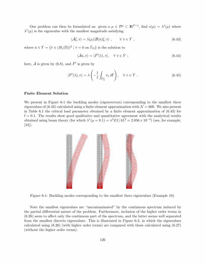
Our problem can then be formulated as: given a µ ∈ Dµ ⊂ IRP=1, find s(µ) = λ1(µ) whereλ1(µ) is the eigenvalue with the smallest magnitude satisfying

〈Aξ, v〉 = λ(µ)〈B(u)ξ, v〉 , ∀ v ∈ Y , (6.43)

where u ∈ Y = v ∈ (H1(Ω))2 | v = 0 on ΓD is the solution to

〈Au, v〉 = 〈F ′(1), v〉, ∀ v ∈ Y ; (6.44)

here, A is given by (6.8), and F ′ is given by

〈F ′(λ), v〉 = λ

(−1t

∫Γn

N

v1 dΓ

), ∀ v ∈ Y . (6.45)

Finite Element Solution

We present in Figure 6-1 the buckling modes (eigenvectors) corresponding to the smallest threeeigenvalues of (6.43) calculated using a finite element approximation withN = 600. We also presentin Table 6.1 the critical load parameter obtained by a finite element approximation of (6.43) fort = 0.1. The results show good qualitative and quantitative agreement with the analytical resultsobtained using beam theory (for which λ1(µ = 0.1) = π2EI/4L2 = 2.056×10−4) (see, for example,[44]).

Figure 6-1: Buckling modes corresponding to the smallest three eigenvalues (Example 10).

Note the smallest eigenvalues are “uncontaminated” by the continuous spectrum induced bythe partial differential nature of the problem. Furthermore, inclusion of the higher order terms in(6.26) seem to affect only the continuous part of the spectrum, and the latter seems well separatedfrom the smallest discrete eigenvalues. This is illustrated in Figure 6-2, in which the eigenvaluescalculated using (6.26) (with higher order terms) are compared with those calculated using (6.27)(without the higher order terms).

126

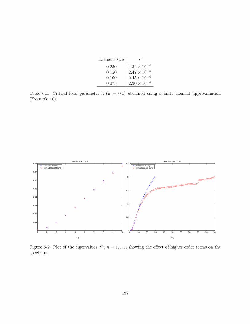
Element size λ1

0.250 4.54× 10−4

0.150 2.47× 10−4

0.100 2.45× 10−4

0.075 2.20× 10−4

Table 6.1: Critical load parameter λ1(µ = 0.1) obtained using a finite element approximation(Example 10).

1 2 3 4 5 6 7 8 9 100

0.01

0.02

0.03

0.04

0.05

0.06

0.07

0.08Element size = 0.25

Classical Theorywith additional terms

0 10 20 30 40 50 60 70 80 90 1000

0.05

0.1

0.15

0.2

0.25Element size = 0.25

Classical Theorywith additional terms

n n

Figure 6-2: Plot of the eigenvalues λn, n = 1, . . . , showing the effect of higher order terms on thespectrum.

127

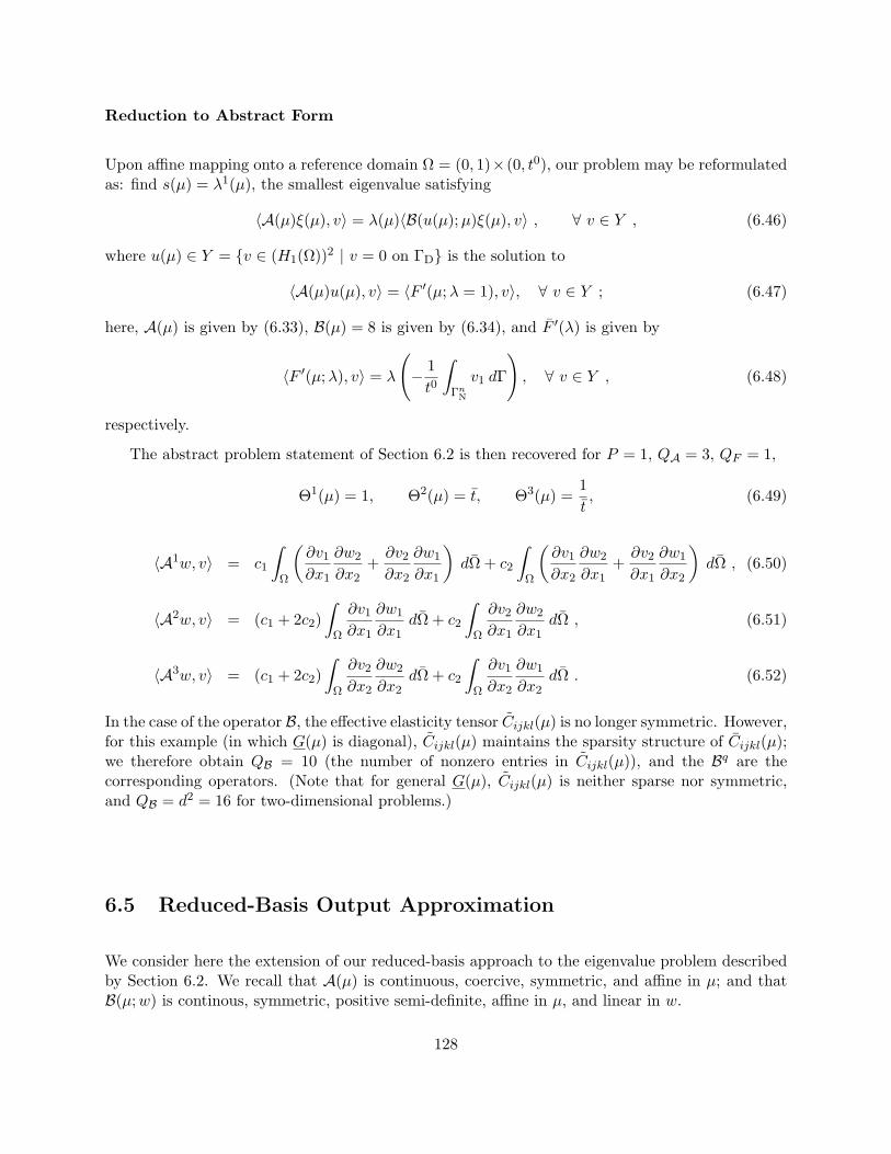
Reduction to Abstract Form

Upon affine mapping onto a reference domain Ω = (0, 1)× (0, t0), our problem may be reformulatedas: find s(µ) = λ1(µ), the smallest eigenvalue satisfying

〈A(µ)ξ(µ), v〉 = λ(µ)〈B(u(µ);µ)ξ(µ), v〉 , ∀ v ∈ Y , (6.46)

where u(µ) ∈ Y = v ∈ (H1(Ω))2 | v = 0 on ΓD is the solution to

〈A(µ)u(µ), v〉 = 〈F ′(µ;λ = 1), v〉, ∀ v ∈ Y ; (6.47)

here, A(µ) is given by (6.33), B(µ) = 8 is given by (6.34), and F ′(λ) is given by

〈F ′(µ;λ), v〉 = λ

(− 1t0

∫Γn

N

v1 dΓ

), ∀ v ∈ Y , (6.48)

respectively.

The abstract problem statement of Section 6.2 is then recovered for P = 1, QA = 3, QF = 1,

Θ1(µ) = 1, Θ2(µ) = t, Θ3(µ) =1t, (6.49)

〈A1w, v〉 = c1

∫Ω

(∂v1∂x1

∂w2

∂x2+∂v2∂x2

∂w1

∂x1

)dΩ + c2

∫Ω

(∂v1∂x2

∂w2

∂x1+∂v2∂x1

∂w1

∂x2

)dΩ , (6.50)

〈A2w, v〉 = (c1 + 2c2)∫

Ω

∂v1∂x1

∂w1

∂x1dΩ + c2

∫Ω

∂v2∂x1

∂w2

∂x1dΩ , (6.51)

〈A3w, v〉 = (c1 + 2c2)∫

Ω

∂v2∂x2

∂w2

∂x2dΩ + c2

∫Ω

∂v1∂x2

∂w1

∂x2dΩ . (6.52)

In the case of the operator B, the effective elasticity tensor Cijkl(µ) is no longer symmetric. However,for this example (in which G(µ) is diagonal), Cijkl(µ) maintains the sparsity structure of Cijkl(µ);we therefore obtain QB = 10 (the number of nonzero entries in Cijkl(µ)), and the Bq are thecorresponding operators. (Note that for general G(µ), Cijkl(µ) is neither sparse nor symmetric,and QB = d2 = 16 for two-dimensional problems.)

6.5 Reduced-Basis Output Approximation

We consider here the extension of our reduced-basis approach to the eigenvalue problem describedby Section 6.2. We recall that A(µ) is continuous, coercive, symmetric, and affine in µ; and thatB(µ;w) is continous, symmetric, positive semi-definite, affine in µ, and linear in w.

128

6.5.1 Approximation Space

We again sample our design space Dµ to create the parameter sample

SµN = µ1, . . . , µN ; (6.53)

we then introduce the reduced-basis spaces

W uN = spanζn = u(µn), n = 1, . . . , N (6.54)

W ξN = spanφn = ξ1(µn), n = 1, . . . , N (6.55)

where we recall ξ1(µ) is the eigenfunction associated with λ1(µ).

Our reduced-order approximation is then: for any µ ∈ Dµ, find uN (µ) ∈W uN such that

〈AuN (µ), v〉 = 〈F (µ), v〉 , ∀ v ∈W uN , (6.56)

and (λN (µ), ξN (µ)) such that

〈A(µ)ξN (µ), v〉 = λN (µ)〈B(µ;uN (µ))ξN (µ), v〉 , ∀ v ∈W ξN ; (6.57)

the output approximation is thensN (µ) = λ1

N (µ) . (6.58)

The dimensions of the reduced-basis spaces for u(µ) and ξ(µ) need not be the same. We notethat the solution to (6.57) is the Galerkin projection onto W ξ

N of the solution to

〈A(µ)ξ′N (µ), v〉 = λ′N (µ)〈B(µ;uN (µ))ξ′N (µ), v〉 , ∀ v ∈ Y ξ ; (6.59)

we have effectively approximated B(µ;u(µ)) in (6.5) with B(µ;uN (µ)) — λN (µ) is therefore anapproximation to λ′N (µ), which in turn approaches λ(µ) only as uN (µ) → u(µ) (and thereforeN →∞).

We also note that λ(µ) may, in general, be negative since B is not strictly positive-definite. Forinstance, structures under pure shear may have “negative” critical load parameters — this impliesthat the buckling occurs when a load reaches the critical value and is applied in the directionopposite to that originally prescribed. In this case, it is not known a priori whether the criticalload parameter is positive or negative; we must therefore approximate both λ1 + and λ1−, the(respectively) positive and negative eigenvalues with the smallest magnitude. We then introduce(in place of W ξ

N ) the reduced-basis spaces

W ξ ±N = spanφ±n = ξ1±(µn), n = 1, . . . , N , (6.60)

and calculate (λ1±N (µ), ξ1±N (µ)) such that

〈A(µ)ξ±N (µ), v〉 = λ±N (µ)〈B(µ;uN (µ))ξN (µ), v〉 , ∀ v ∈W ξN ; (6.61)

the output approximation is thensN (µ) = λ1±

N (µ) . (6.62)

129

6.5.2 Offline/Online Computational Decomposition

We now develop off-line/on-line computational procedures that exploit this dimension reduction.

We first express our approximation uN (µ) ∈ Y to be a linear combination of the appropriatebasis functions,

uN (µ) =N∑

j=1

uN j(µ) ζj (6.63)

where uN (µ) ∈ IRN ; we then choose for test functions v = ζi, i = 1, . . . , N . Inserting theserepresentations into (6.56) yields the desired algebraic equations for uN (µ) ∈ IRN ,

AuN (µ) uN (µ) = FN . (6.64)

Here AuN (µ) ∈ IRN×N is the symmetric positive-definite (SPD) matrix with entries

AuN i,j(µ) ≡ 〈A(µ)ζj , ζi〉, 1 ≤ i, j ≤ N , (6.65)

and FN ∈ IRN is the “load” vector with entries

FN i ≡ 〈F (µ), ζi〉, 1 ≤ i ≤ N . (6.66)

We also express our approximation ξN (µ) ∈ Y to be a linear combination of the correspondingbasis functions,

ξN (µ) =N∑

j=1

ξN j(µ) φj , (6.67)

where ξN

(µ) ∈ IRN . Then, in (6.57), we choose for test functions v = φi, i = 1, . . . , N , andapproximate u(µ) by uN (µ), yielding

AξN (µ) ξ

N(µ) = BN (µ;uN (µ)) . (6.68)

Here AξN (µ) ∈ IRN×N is the symmetric positive-definite (SPD) matrix with entries

AξN i,j(µ) ≡ 〈A(µ)φj , φi〉, 1 ≤ i, j ≤ N , (6.69)

and BN (µ;uN (µ)) ∈ IRN×N is the symmetric positive semi-definite (SPSD) matrix with entries

BN i,j(µ;uN (µ)) ≡ 〈B(µ;uN (µ))φj , φi〉, (6.70)

=N∑

n=1

uN n(µ)〈B(µ; ζn)φj , φi〉, 1 ≤ i, j ≤ N . (6.71)

130

We now invoke (6.1)-(6.3) to write

AuN i,j(µ) =

QA∑q=1

Θq(µ) 〈Aqζj , ζi〉 , (6.72)

AξN i,j(µ) =

QA∑q=1

Θq(µ) 〈Aqφj , φi〉 , (6.73)

BN i,j(µ;uN (µ)) =N∑

n=1

QB∑q=1

uN n(µ) ΘqB(µ) 〈Bq(µ; ζn)φj , φi〉 (6.74)

FN i(µ) =QF∑q=1

ϕqF (µ) 〈F q, ζi〉 ; (6.75)

or, more concisely,

AuN (µ) =

QA∑q=1

Θq(µ)Au qN , (6.76)

AξN (µ) =

QA∑q=1

Θq(µ)Aξ qN , (6.77)

(6.78)

BN (µ;uN (µ)) =N∑

n=1

B∑q=1

ΘqB(µ) uN n(µ)Bqn

N , (6.79)

FN (µ) =QF∑q=1

αqF (µ) F q

N , (6.80)

where the Au qN ∈ IRN×N , Aξ q

N ∈ IRN×N , BqnN ∈ IRN×N , and F q

N ∈ IRN , are given by

Au qN i,j = 〈Aqζj , ζi〉 , 1 ≤ i, j ≤ N, 1 ≤ q ≤ QA , (6.81)

Aξ qN i,j = 〈Aqφj , φi〉 , 1 ≤ i, j ≤ N, 1 ≤ q ≤ QA , (6.82)

BqnN i,j = 〈Bq(ζn)φj , φi〉 , 1 ≤ i, j, n ≤ N, 1 ≤ q ≤ QB , (6.83)

F qN i = 〈F q, ζi〉 , 1 ≤ i ≤ N, 1 ≤ q ≤ QF , (6.84)

Hence, in the off-line stage, we compute the u(µn) and ξ(µn), and form the Au qN , Aξ q

N , BqnN ,

and FN : this requires N (expensive) finite element solutions of the equilibrium equation andthe generalized eigenvalue problem, as well as O(QBN3) + O(2QAN2) + O(QFN) finite-element-vector inner products. In the on-line stage, for any given new µ, we first form Au

N (µ) and FN (µ)from (6.76) and (6.80), respectively, then solve (6.64) for uN (µ); we subsequently form Aξ

N (µ) andBN (µ;uN (µ)) from (6.77)-(6.79), then solve (6.68) for ξ

N(µ), and finally evaluate sN (µ) = λ1

N (µ):

131

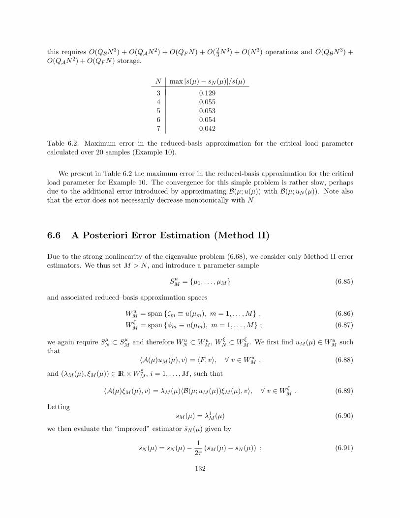
this requires O(QBN3) + O(QAN2) + O(QFN) + O(23N

3) + O(N3) operations and O(QBN3) +O(QAN2) +O(QFN) storage.

N max |s(µ)− sN (µ)|/s(µ)

3 0.1294 0.0555 0.0536 0.0547 0.042

Table 6.2: Maximum error in the reduced-basis approximation for the critical load parametercalculated over 20 samples (Example 10).

We present in Table 6.2 the maximum error in the reduced-basis approximation for the criticalload parameter for Example 10. The convergence for this simple problem is rather slow, perhapsdue to the additional error introduced by approximating B(µ;u(µ)) with B(µ;uN (µ)). Note alsothat the error does not necessarily decrease monotonically with N .

6.6 A Posteriori Error Estimation (Method II)

Due to the strong nonlinearity of the eigenvalue problem (6.68), we consider only Method II errorestimators. We thus set M > N , and introduce a parameter sample

SµM = µ1, . . . , µM (6.85)

and associated reduced–basis approximation spaces

W uM = span ζm ≡ u(µm), m = 1, . . . ,M , (6.86)

W ξM = span φm ≡ u(µm), m = 1, . . . ,M ; (6.87)

we again require SµN ⊂ Sµ

M and therefore W uN ⊂W u

M , W ξN ⊂W ξ

M . We first find uM (µ) ∈W uM such

that〈A(µ)uM (µ), v〉 = 〈F, v〉, ∀ v ∈W u

M , (6.88)

and (λM (µ), ξM (µ)) ∈ IR×W ξM , i = 1, . . . ,M , such that

〈A(µ)ξM (µ), v〉 = λM (µ)〈B(µ;uM (µ))ξM (µ), v〉, ∀ v ∈W ξM . (6.89)

LettingsM (µ) = λ1

M (µ) (6.90)

we then evaluate the “improved” estimator sN (µ) given by

sN (µ) = sN (µ)− 12τ

(sM (µ)− sN (µ)) ; (6.91)

132

our lower and upper output estimators are then

s−N (µ) = sN (µ)− 12∆N (µ) (6.92)

s+N (µ) = sN (µ) +12∆N (µ) (6.93)

where ∆N (µ), the estimator for the error |s(µ)− sN (µ)|, is given by

∆N,M (µ) =1τ|sM (µ)− sN (µ)| (6.94)

for some τ ∈ (0, 1). The effectivity of the approximation is defined as

ηN,M (µ) =∆N,M (µ)

s(µ)− sN (µ). (6.95)

We shall once again consider M = 2N .

N min ηN (µ) max ηN (µ)

1 1.9773 2.00992 1.7067 2.33953 1.8811 2.81514 1.9772 2.2783

Table 6.3: Minimum and maximum effectivities for Method II error estimators (with τ = 0.5)calculated over 20 samples (Example 10).

The analysis of the bounding properties of Method II estimators presented in Section 5.8.2 alsoapplies here. However, the necessary hypothesis (4.190), while still plausible, is now less so than inChapters 4 and 5. Nevertheless, the effectivity results presented in Table 6.3 show that ηN (µ) stilltends to 1/τ .

133

134

Chapter 7

Reduced-Basis Methods for Analysis,Optimization, and Prognosis:A MicroTruss Example

7.1 Introduction

In Chapters 3 through 6 we present the reduced-basis method — a technique for the rapid andreliable prediction of linear-functional outputs of partial differential equations with affine parameterdependence. Reduced–basis output bound methods are intended to render partial–differential-equation solutions truly useful: essentially real–time as regards operation count; “blackbox” asregards reliability; and directly relevant as regards the (limited) input–output data required.

In this chapter we revisit the microtruss example presented in Chapter 1, focusing on the struc-tural (solid mechanics) aspects of the problem. We apply reduced-basis methods to the predictionof the relevant outputs of interest; we then illustrate how these methods directly enable rapid andreliable solution of “real” optimization problems — even in the presence of significant uncertainty.In particular, we employ reduced-basis output bounds in the context of (i) design — optimizinga system at conception with respect to prescribed objectives, constraints, and worst-case environ-mental conditions — and (ii) prognosis — optimizing a system during operation subject to evolvingsystem characteristics, dynamic system requirements, and changing environmental conditions.

7.2 Formulation

We begin with the formulation of the microtruss problem, focusing particularly on the structuralaspects. In Sections 7.2.1 and 7.2.2, the circumflex ( ) denotes dimensional quantities, and indicestake the values 1, . . . , d.

7.2.1 Dimensional Formulation

We consider the periodic open cellular structure shown in Figure 7-1. As indicated in Chapter 1,the structure is simultaneously designed for heat-transfer as well as structural capability; we shallfocus on the latter. The prismatic microtruss consists of a frame (upper, lower, and lateral faces)and a core of trusses. The structure transmits a force per unit depth F uniformly distributed

135

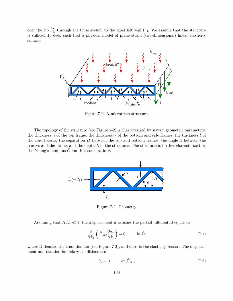
over the tip ΓtN through the truss system to the fixed left wall ΓD. We assume that the structure

is sufficiently deep such that a physical model of plane strain (two-dimensional) linear elasticitysuffices.

load

heat, q′′

coolant Phigh, T0

Plow

ft

ΓS

ΓtN

Γflux

Figure 7-1: A microtruss structure.

The topology of the structure (see Figure 7-2) is characterized by several geometric parameters:the thickness tt of the top frame, the thickness tb of the bottom and side frames, the thickness t ofthe core trusses, the separation H between the top and bottom frames, the angle α between thetrusses and the frame, and the depth L of the structure. The structure is further characterized bythe Young’s modulus C and Poisson’s ratio ν.

tb

ttt

αHts(= tb)

Figure 7-2: Geometry

Assuming that H/L 1, the displacement u satisfies the partial differential equation

∂

∂xj

(Cijkl

∂uk

∂xl

)= 0, in Ω, (7.1)

where Ω denotes the truss domain (see Figure 7-2), and Cijkl is the elasticity tensor. The displace-ment and traction boundary conditions are

ui = 0 , on ΓD , (7.2)

136

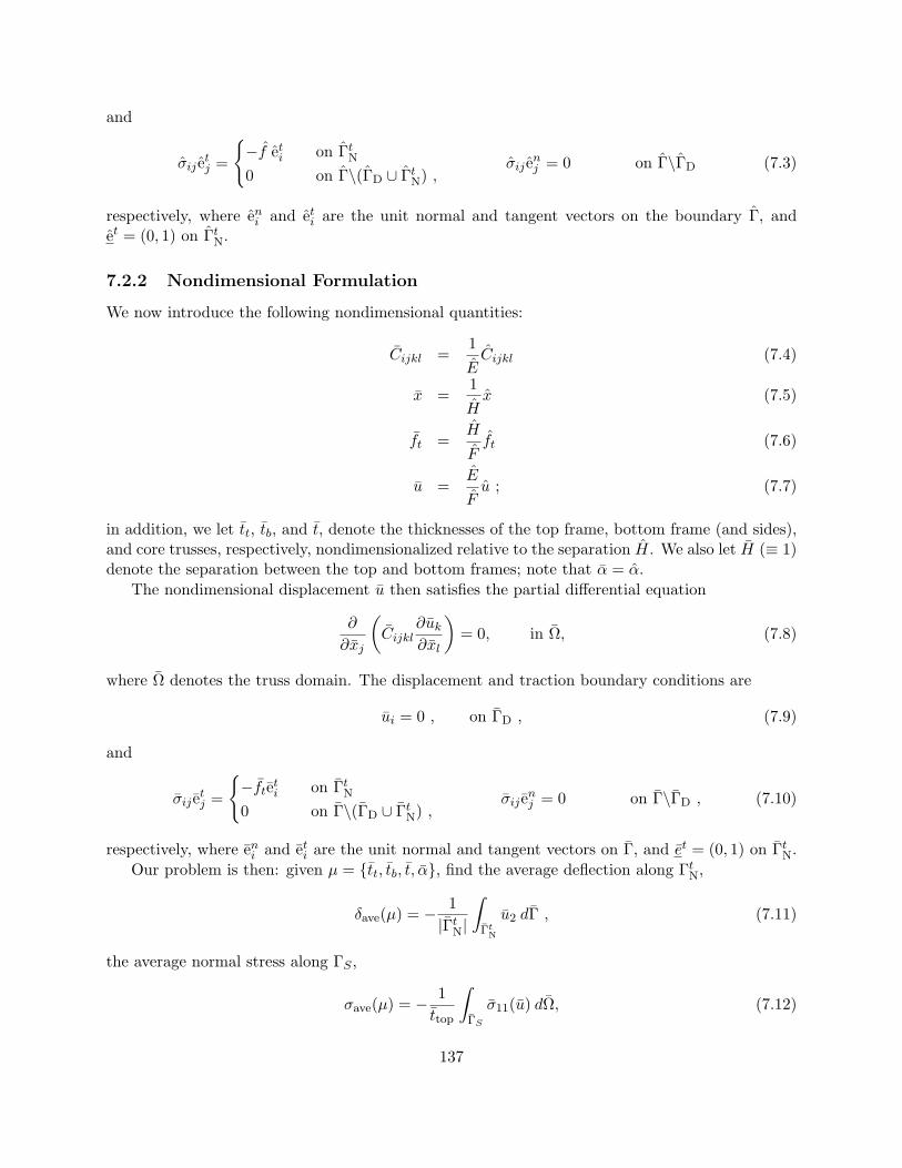
and

σij etj =

−f et

i on ΓtN

0 on Γ\(ΓD ∪ ΓtN) ,

σij enj = 0 on Γ\ΓD (7.3)

respectively, where eni and et

i are the unit normal and tangent vectors on the boundary Γ, andet = (0, 1) on Γt

N.

7.2.2 Nondimensional Formulation

We now introduce the following nondimensional quantities:

Cijkl =1ECijkl (7.4)

x =1Hx (7.5)

ft =H

Fft (7.6)

u =E

Fu ; (7.7)

in addition, we let tt, tb, and t, denote the thicknesses of the top frame, bottom frame (and sides),and core trusses, respectively, nondimensionalized relative to the separation H. We also let H (≡ 1)denote the separation between the top and bottom frames; note that α = α.

The nondimensional displacement u then satisfies the partial differential equation

∂

∂xj

(Cijkl

∂uk

∂xl

)= 0, in Ω, (7.8)

where Ω denotes the truss domain. The displacement and traction boundary conditions are

ui = 0 , on ΓD , (7.9)

and

σij etj =

−ftet

i on ΓtN

0 on Γ\(ΓD ∪ ΓtN) ,

σij enj = 0 on Γ\ΓD , (7.10)

respectively, where eni and et

i are the unit normal and tangent vectors on Γ, and et = (0, 1) on ΓtN.

Our problem is then: given µ = tt, tb, t, α, find the average deflection along ΓtN,

δave(µ) = − 1|Γt

N|

∫Γt

N

u2 dΓ , (7.11)

the average normal stress along ΓS ,

σave(µ) = − 1ttop

∫ΓS

σ11(u) dΩ, (7.12)

137

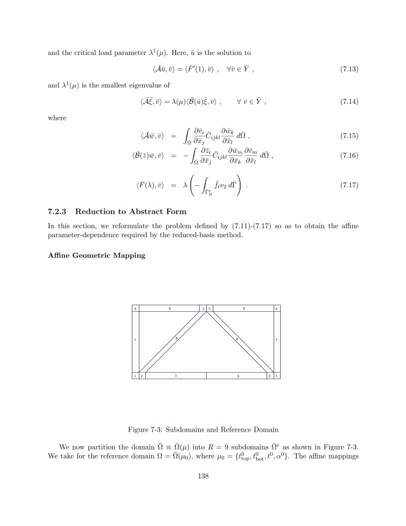
and the critical load parameter λ1(µ). Here, u is the solution to

〈Au, v〉 = 〈F ′(1), v〉 , ∀v ∈ Y , (7.13)

and λ1(µ) is the smallest eigenvalue of

〈Aξ, v〉 = λ(µ)〈B(u)ξ, v〉 , ∀ v ∈ Y , (7.14)

where

〈Aw, v〉 =∫

Ω

∂vi

∂xjCijkl

∂wk

∂xldΩ , (7.15)

〈B(z)w, v〉 = −∫

Ω

∂zi∂xj

Cijkl∂wm

∂xk

∂vm

∂xldΩ , (7.16)

〈F (λ), v〉 = λ

(−∫

ΓtN

ftv2 dΓ

). (7.17)

7.2.3 Reduction to Abstract Form

In this section, we reformulate the problem defined by (7.11)-(7.17) so as to obtain the affineparameter-dependence required by the reduced-basis method.

Affine Geometric Mapping

2 2 3

4 4 6 6

7 8 9

1

7

3 1

5 5

Figure 7-3: Subdomains and Reference Domain

We now partition the domain Ω ≡ Ω(µ) into R = 9 subdomains Ωr as shown in Figure 7-3.We take for the reference domain Ω = Ω(µ0), where µ0 = t0top, t0bot, t

0, α0. The affine mappings

138

Gr(µ) : Ωr → Ωr are then given by Gr(µ; x) = Gr(µ)x+ br(µ), where

G1 =

[t0sts

0

0 t0bottbot

]G2 =

t0hth

0

0 t0bottbot

G3 =

[L0

L0

0 t0bottbot

](7.18)

G4 =

t0sts

0

0t0topttop

G5 =

t0hth

0

0t0topttop

G6 =

[L0

L0

0t0topttop

](7.19)

G7 =

[t0sts

00 H0

H

](7.20)

G8 =[1 − tanα0

0 1

][ t0hth

00 H0

H

] [1 tan α0 1

](7.21)

G9 =[1 tanα0

0 1

][ t0hth

00 H0

H

] [1 − tan α0 1

], (7.22)

where the ts = tbot is the thickness of the side trusses; th = t/ sin α is the horizontal thickness ofthe diagonal trusses; and L = H/ tan α; similar formulas apply for t0s , t

0h, and L0.

We recall that the affine decomposition of the linear elasticity operator is related to the numberof elements in the elasticity tensor. It would therefore seem that for our microtruss example QAmight be very large — as large as 144, or the number of elements in Cijkl(µ) (16) times the numberof subdomains (9). However, as illustrated in Examples 1-9 of Chapters 3 and 5, the symmetry andsparsity of the elasticity tensor may be exploited to reduce QA. In particular, we consider only thenonzero, unique elements of the Cr

ijkl(µ), thus reducing QA to [(3×7)+(10×2)] = 41; the first termcorresponds to the 7 subdomains undergoing only “stretch” transformations (r = 1, . . . , 7) while thesecond term coresponds to the 2 subdomains undergoing both “stretch” and “shear.” Furthermore,we can further reduce QA by consolidating those terms among all the (unique,nonzero) elementsof the Cr

ijkl(µ) which are the same. For example, we consider subdomains 1 through 7 for whichthe elements of the elasticity tensor are given in Table 7.1, where we αx = G11 and αy = G22

are the diagonal (nonzero) elements of the mapping matrix G. We then note that Cr1122(µ) = c1

and Cr1221(µ) = c2 for r = 1, . . . , 7. Taking this into consideration, QA is further reduced to

[1 + (2 × 7) + (10 × 2)] = 35. Further reductions can be obtained by making similar observationsfor r = 8, 9.

Reference Domain Formulation

Using the results obtained in Chapters 5 and 6, our problem may be reformulated as: for any givenµ = tt, tb, t, α ∈ Dµ = [0.22, 2.2]3 × [0, 45], find

δave(µ) = − 1tt + tb + H

∫Γt

N

u2|G−1(µ)et| dΓ , (7.23)

139

ij\kl 11 12 21 22

11αx

αy(c1 + 2c2) 0 0 1(c1)

12 · αy

αx(c2) 1(c2) 0

21 · · αx

αy(c2) 0

22 · · · αy

αx(c1 + 2c2)

Table 7.1: Elements of the effective elasticity tensor for subdomains undergoing a ”stretch” trans-formation.

the average normal stress along ΓS (near the support),

σave(µ) = − 1ttop

∫ΓS

σ11(u) dΓ, (7.24)

and the critical (positive and negative) load parameters, λ1±(µ). Here, u is the solution to

〈A(µ)u(µ), v〉 = 〈F ′(µ; 1), v〉 , ∀ v ∈ Y , (7.25)

and λ1±(µ) are the smallest positive and negative eigenvalues satisfying

〈A(µ)ξ(µ), v〉 = λ(µ)〈B(u(µ);µ)ξ(µ), v〉 , ∀ v ∈ Y , (7.26)

where

〈A(µ)w, v〉 =R∑

r=1

∫Ωr

∂wi

∂xjCr

ijkl(µ)∂vk

∂xl∀ w, v ∈ Y , (7.27)

〈B(z)w, v〉 = −R∑

r=1

∫Ω

∂zi∂xj

Cijkl∂wm

∂xk

∂vm

∂xldΩ , (7.28)

〈F ′(µ;λ), v〉 = λ

R∑r=1

(∫Γt r

N

f t r(µ)v2 dΓ

). (7.29)

Here Crijkl(µ) = Cr

ijkl(µ) = Grjj′(µ) Cr

ij′kl′ Grll′(µ) det(Gr(µ))−1, f t r

i (µ) is given by

f t ri (µ) = ft r et

i

∣∣(Gr(µ))−1 et∣∣ , (7.30)

and Y (Ω) = v ∈(H1(Ω)

)2 | vieni = 0 on Γn

D, vieti = 0 on Γt

D.

7.3 Analysis

In this section we (i) examine the convergence of the reduced-basis approximation and the effectivityof the (Method II) error estimator for the microtruss example; and (ii) investigate the behavior of

140

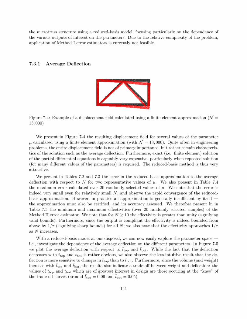
the microtruss structure using a reduced-basis model, focusing particularly on the dependence ofthe various outputs of interest on the parameters. Due to the relative complexity of the problem,application of Method I error estimators is currently not feasible.

7.3.1 Average Deflection

Figure 7-4: Example of a displacement field calculated using a finite element approximation (N =13, 000)

We present in Figure 7-4 the resulting displacement field for several values of the parameterµ calculated using a finite element approximation (with N = 13, 000). Quite often in engineeringproblems, the entire displacement field is not of primary importance, but rather certain characteris-tics of the solution such as the average deflection. Furthermore, exact (i.e., finite element) solutionof the partial differential equations is arguably very expensive, particularly when repeated solution(for many different values of the parameters) is required. The reduced-basis method is thus veryattractive.

We present in Tables 7.2 and 7.3 the error in the reduced-basis approximation to the averagedeflection with respect to N for two representative values of µ. We also present in Table 7.4the maximum error calculated over 20 randomly selected values of µ. We note that the error isindeed very small even for relatively small N , and observe the rapid convergence of the reduced-basis approximation. However, in practice an approximation is generally insufficient by itself —the approximation must also be certified, and its accuracy assessed. We therefore present in inTable 7.5 the minimum and maximum effectivities (over 20 randomly selected samples) of theMethod II error estimator. We note that for N ≥ 10 the effectivity is greater than unity (signifyingvalid bounds). Furthermore, since the output is compliant the effectivity is indeed bounded fromabove by 1/τ (signifying sharp bounds) for all N ; we also note that the effectivity approaches 1/τas N increases.

With a reduced-basis model at our disposal, we can now easily explore the parameter space —i.e., investigate the dependence of the average deflection on the different parameters. In Figure 7-5we plot the average deflection with respect to ttop and tbot. While the fact that the deflectiondecreases with ttop and tbot is rather obvious, we also observe the less intuitive result that the de-flection is more sensitive to changes in ttop than to tbot. Furthermore, since the volume (and weight)increase with ttop and tbot, the results also indicate a trade-off between weight and deflection: thevalues of ttop and tbot which are of greatest interest in design are those occuring at the “knee” ofthe trade-off curves (around ttop = 0.06 and tbot = 0.05).

141

N |s(µ)−sN (µ)|s(µ)

∆N (µ)s(µ) ηN (µ)

10 5.49e-02 8.10e-02 1.4820 1.44e-02 2.48e-02 1.7230 4.84e-03 9.00e-03 1.8640 2.00e-03 3.90e-03 1.9450 9.57e-04 1.84e-03 1.9260 3.51e-04 6.58e-04 1.8770 1.19e-04 2.08e-04 1.7580 5.39e-05 9.20e-05 1.7190 4.15e-05 7.56e-05 1.82100 3.38e-05 6.26e-05 1.85

Table 7.2: Error and effectivities for the deflection for µ = µ0 (the reference parameter).

N |s(µ)− sN (µ)|/s(µ) ∆N (µ)/s(µ) ηN (µ)

10 3.67e-01 7.02e-01 1.9120 1.64e-02 2.38e-02 1.4530 7.89e-03 1.30e-02 1.6440 4.46e-03 8.22e-03 1.8450 2.16e-03 4.10e-03 1.9060 1.41e-03 2.70e-03 1.9270 5.85e-04 1.10e-03 1.8980 3.50e-04 6.66e-04 1.9190 1.21e-04 2.22e-04 1.83100 1.10e-04 2.06e-04 1.88

Table 7.3: Error and effectivities for the deflection for a randomly selected value of µ.

N max(s(µ)− sN (µ))/s(µ)

10 4.80e-0120 2.80e-0140 1.40e-0260 6.80e-0380 1.50e-03100 1.10e-03

Table 7.4: Maximum error in the deflectioncalculated over 20 randomly selected valuesof µ.

N min ηN (µ) max ηN (µ)

10 0.66 1.8720 1.36 1.9840 1.52 1.9760 1.26 1.9980 1.55 2.00

100 1.64 2.00

Table 7.5: Minimum and maximum effectivi-ties for the deflection calculated over 20 ran-domly selected values of µ.

142

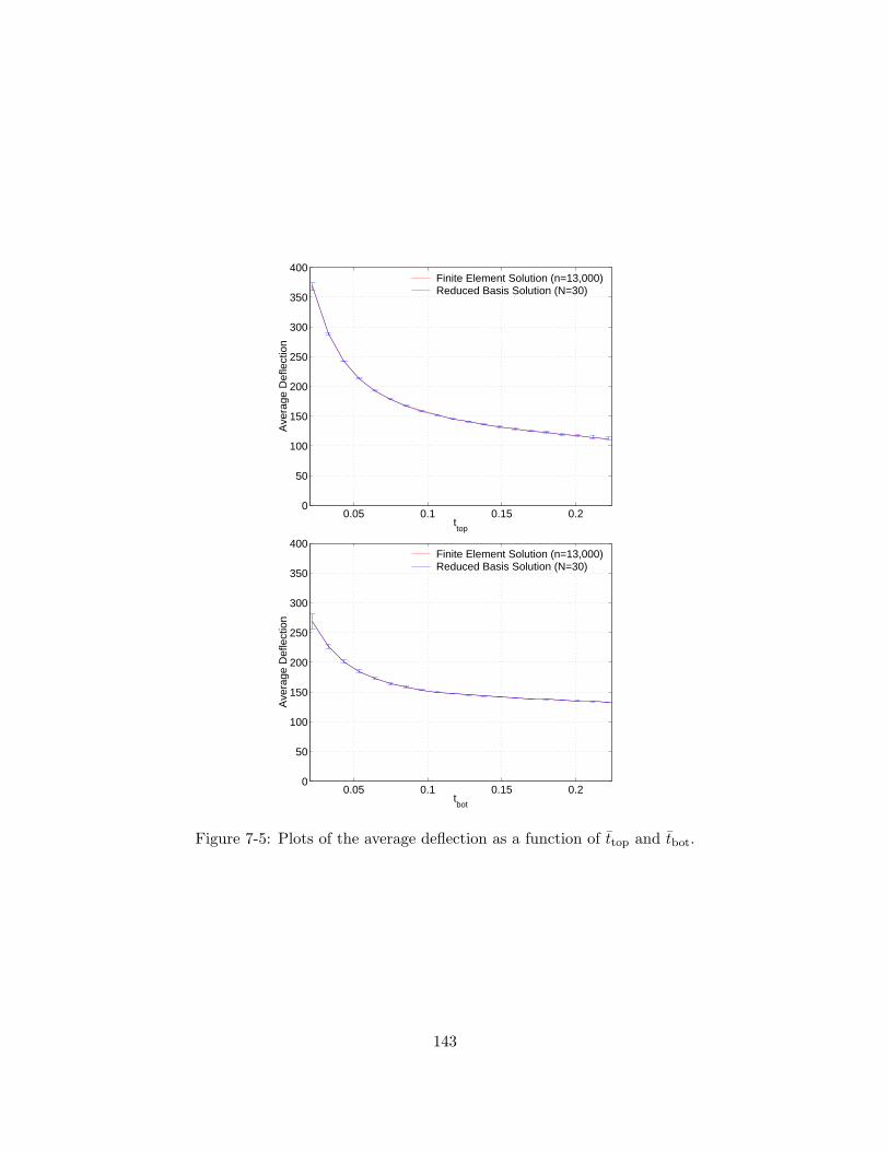
0.05 0.1 0.15 0.20

50

100

150

200

250

300

350

400

ttop

Ave

rage

Def

lect

ion

Finite Element Solution (n=13,000)Reduced Basis Solution (N=30)

0.05 0.1 0.15 0.20

50

100

150

200

250

300

350

400

tbot

Ave

rage

Def

lect

ion

Finite Element Solution (n=13,000)Reduced Basis Solution (N=30)

Figure 7-5: Plots of the average deflection as a function of ttop and tbot.

143

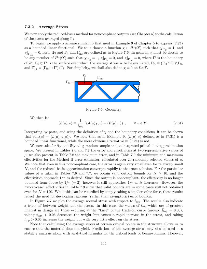
7.3.2 Average Stress

We now apply the reduced-basis method for noncompliant outputs (see Chapter 5) to the calculationof the stress averaged along ΓS .

To begin, we apply a scheme similar to that used in Example 9 of Chapter 5 to express (7.24)as a bounded linear functional. We thus choose a function χ ∈ H1(Ω′) such that χ|ΓS

= 1, andχ|Γ′int

= 0; here, ΩS and ΓS and Γ′int are defined as in Figure 7-6. In general, χ must be chosen tobe any member of H1(Ω′) such that χ|ΓS

= 1, χ|Γ′D = 0, and χ|Γ′int= 0, where Γ′ is the boundary

of Ω′, ΓS ⊂ Γ′ is the surface over which the average stress is to be evaluated, Γ′D ≡ (ΓD ∩ Γ′)\ΓS,and Γ′int ≡ (Γint ∩ Γ′)\ΓS. For simplicity, we shall also define χ ≡ 0 on Ω\Ω′.

ΓS

Γ′int

Ω′

Figure 7-6: Geometry

We then let〈L(µ), v〉 ≡ 1

ttop(〈A(µ)χ, v〉 − 〈F (µ), v〉) , ∀ v ∈ Y . (7.31)

Integrating by parts, and using the definition of χ and the boundary conditions, it can be shownthat σave(µ) = 〈L(µ), u(µ)〉. We note that as in Example 9, 〈L(µ), v〉 defined as in (7.31) is abounded linear functional, while the more obvious alternative in (7.24) is not.

We now take for SN and WN a log-random sample and an integrated primal-dual approximationspace. We present in Tables 7.6 and 7.7 the error and effectivities at two representative values ofµ; we also present in Table 7.8 the maximum error, and in Table 7.9 the minimum and maximumeffectivities for the Method II error estimator, calculated over 20 randomly selected values of µ.We note that even in this noncompliant case, the error is again very small even for relatively smallN , and the reduced-basis approximation converges rapidly to the exact solution. For the particularvalues of µ taken in Tables 7.6 and 7.7, we obtain valid output bounds for N ≥ 10, and theeffectivities approach 1/τ as desired. Since the output is noncompliant, the effectivity is no longerbounded from above by 1/τ (= 2); however it still approaches 1/τ as N increases. However, the“worst-case” effectivities in Table 7.9 show that valid bounds are in some cases still not obtainedeven for N = 120. While this can be remedied by simply taking a smaller value for τ , these resultsreflect the need for developing rigorous (rather than asymptotic) error bounds.

In Figure 7-7 we plot the average normal stress with respect to ttop. The results also indicatea trade-off between weight and the stress. In this case, the values of ttop which are of greatestinterest in design are those occuring at the “knee” of the trade-off curve (around ttop = 0.06);taking ttop < 0.06 decreases the weight but causes a rapid increase in the stress, and takingttop > 0.06 increases the weight but with very little effect on the stress.

Note that calculating the average stress at certain critical points in the structure allows us toensure that the material does not yield. Predictions of the average stress may also be used in astability analysis along with analytical formulas for the critical loads of beam-columns. However,

144

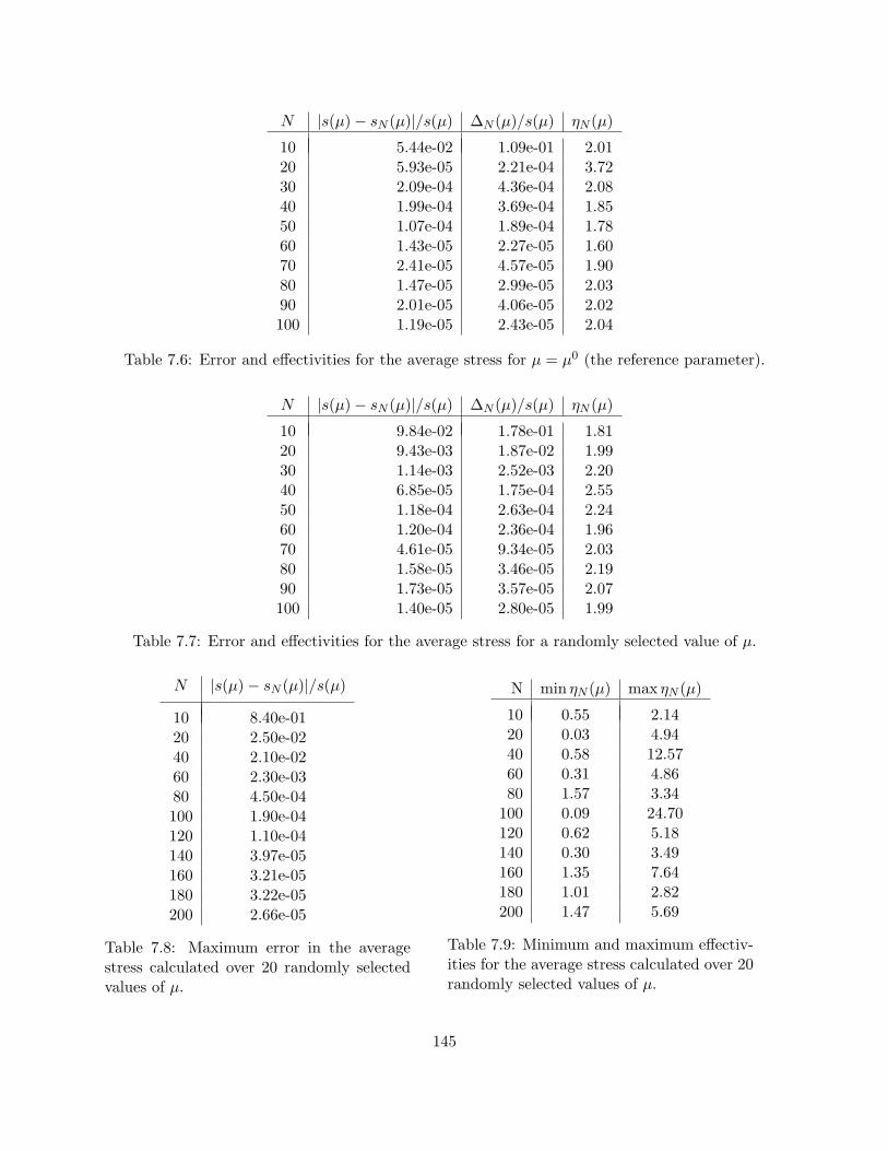
N |s(µ)− sN (µ)|/s(µ) ∆N (µ)/s(µ) ηN (µ)

10 5.44e-02 1.09e-01 2.0120 5.93e-05 2.21e-04 3.7230 2.09e-04 4.36e-04 2.0840 1.99e-04 3.69e-04 1.8550 1.07e-04 1.89e-04 1.7860 1.43e-05 2.27e-05 1.6070 2.41e-05 4.57e-05 1.9080 1.47e-05 2.99e-05 2.0390 2.01e-05 4.06e-05 2.02100 1.19e-05 2.43e-05 2.04

Table 7.6: Error and effectivities for the average stress for µ = µ0 (the reference parameter).

N |s(µ)− sN (µ)|/s(µ) ∆N (µ)/s(µ) ηN (µ)

10 9.84e-02 1.78e-01 1.8120 9.43e-03 1.87e-02 1.9930 1.14e-03 2.52e-03 2.2040 6.85e-05 1.75e-04 2.5550 1.18e-04 2.63e-04 2.2460 1.20e-04 2.36e-04 1.9670 4.61e-05 9.34e-05 2.0380 1.58e-05 3.46e-05 2.1990 1.73e-05 3.57e-05 2.07100 1.40e-05 2.80e-05 1.99

Table 7.7: Error and effectivities for the average stress for a randomly selected value of µ.

N |s(µ)− sN (µ)|/s(µ)

10 8.40e-0120 2.50e-0240 2.10e-0260 2.30e-0380 4.50e-04100 1.90e-04120 1.10e-04140 3.97e-05160 3.21e-05180 3.22e-05200 2.66e-05

Table 7.8: Maximum error in the averagestress calculated over 20 randomly selectedvalues of µ.

N min ηN (µ) max ηN (µ)

10 0.55 2.1420 0.03 4.9440 0.58 12.5760 0.31 4.8680 1.57 3.34

100 0.09 24.70120 0.62 5.18140 0.30 3.49160 1.35 7.64180 1.01 2.82200 1.47 5.69

Table 7.9: Minimum and maximum effectiv-ities for the average stress calculated over 20randomly selected values of µ.

145

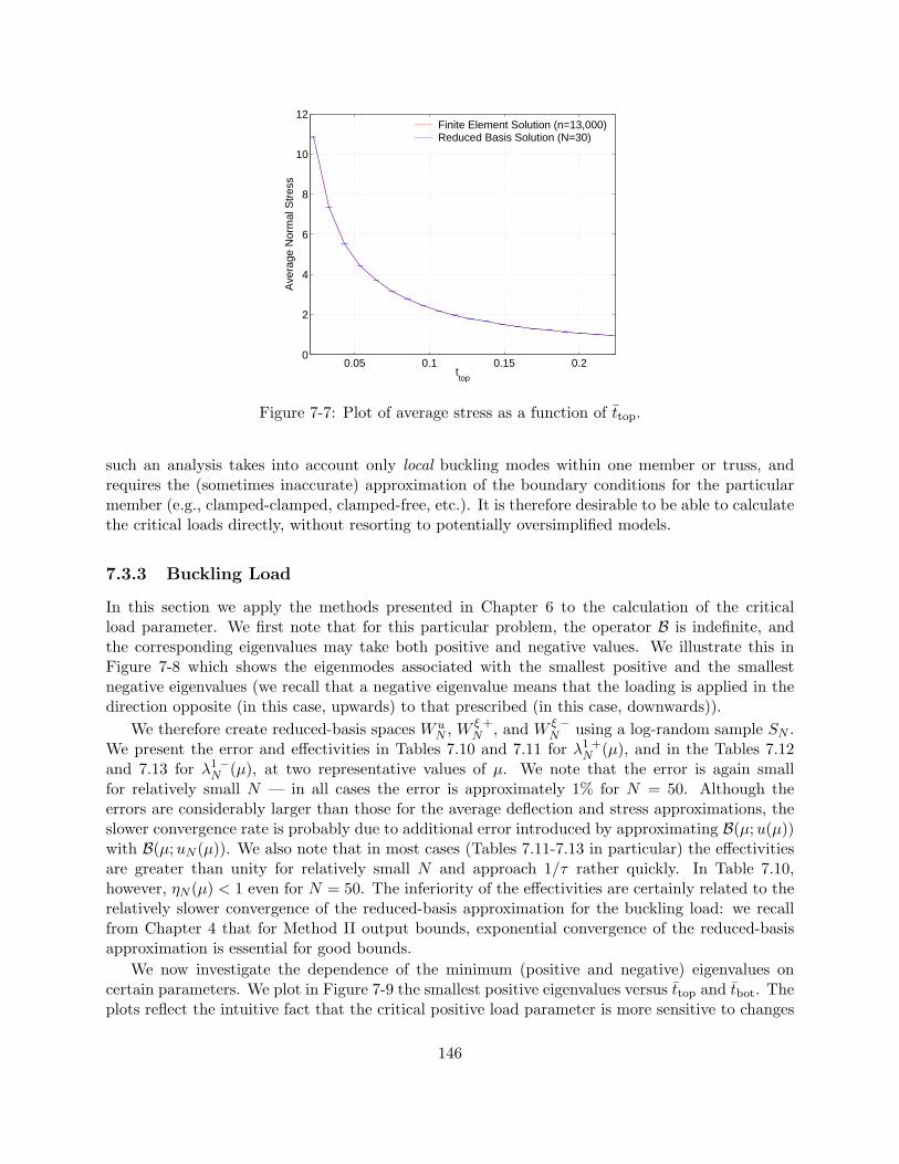
0.05 0.1 0.15 0.20

2

4

6

8

10

12

ttop

Ave

rage

Nor

mal

Str

ess

Finite Element Solution (n=13,000)Reduced Basis Solution (N=30)

Figure 7-7: Plot of average stress as a function of ttop.

such an analysis takes into account only local buckling modes within one member or truss, andrequires the (sometimes inaccurate) approximation of the boundary conditions for the particularmember (e.g., clamped-clamped, clamped-free, etc.). It is therefore desirable to be able to calculatethe critical loads directly, without resorting to potentially oversimplified models.

7.3.3 Buckling Load

In this section we apply the methods presented in Chapter 6 to the calculation of the criticalload parameter. We first note that for this particular problem, the operator B is indefinite, andthe corresponding eigenvalues may take both positive and negative values. We illustrate this inFigure 7-8 which shows the eigenmodes associated with the smallest positive and the smallestnegative eigenvalues (we recall that a negative eigenvalue means that the loading is applied in thedirection opposite (in this case, upwards) to that prescribed (in this case, downwards)).

We therefore create reduced-basis spaces W uN , W ξ +

N , and W ξ −N using a log-random sample SN .

We present the error and effectivities in Tables 7.10 and 7.11 for λ1 +N (µ), and in the Tables 7.12

and 7.13 for λ1−N (µ), at two representative values of µ. We note that the error is again small

for relatively small N — in all cases the error is approximately 1% for N = 50. Although theerrors are considerably larger than those for the average deflection and stress approximations, theslower convergence rate is probably due to additional error introduced by approximating B(µ;u(µ))with B(µ;uN (µ)). We also note that in most cases (Tables 7.11-7.13 in particular) the effectivitiesare greater than unity for relatively small N and approach 1/τ rather quickly. In Table 7.10,however, ηN (µ) < 1 even for N = 50. The inferiority of the effectivities are certainly related to therelatively slower convergence of the reduced-basis approximation for the buckling load: we recallfrom Chapter 4 that for Method II output bounds, exponential convergence of the reduced-basisapproximation is essential for good bounds.

We now investigate the dependence of the minimum (positive and negative) eigenvalues oncertain parameters. We plot in Figure 7-9 the smallest positive eigenvalues versus ttop and tbot. Theplots reflect the intuitive fact that the critical positive load parameter is more sensitive to changes

146

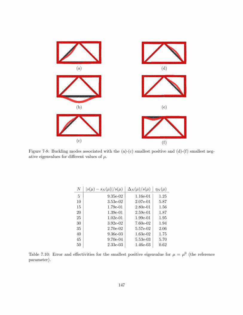
(a)

(b)

(c)

(d)

(e)

(f)

Figure 7-8: Buckling modes associated with the (a)-(c) smallest positive and (d)-(f) smallest neg-ative eigenvalues for different values of µ.

N |s(µ)− sN (µ)|/s(µ) ∆N (µ)/s(µ) ηN (µ)

5 9.35e-02 1.16e-01 1.2510 3.53e-02 2.07e-01 5.8715 1.79e-01 2.80e-01 1.5620 1.39e-01 2.59e-01 1.8725 1.02e-01 1.99e-01 1.9530 3.92e-02 7.60e-02 1.9435 2.70e-02 5.57e-02 2.0640 9.36e-03 1.63e-02 1.7545 9.70e-04 5.53e-03 5.7050 2.33e-03 1.46e-03 0.62

Table 7.10: Error and effectivities for the smallest positive eigenvalue for µ = µ0 (the referenceparameter).

147

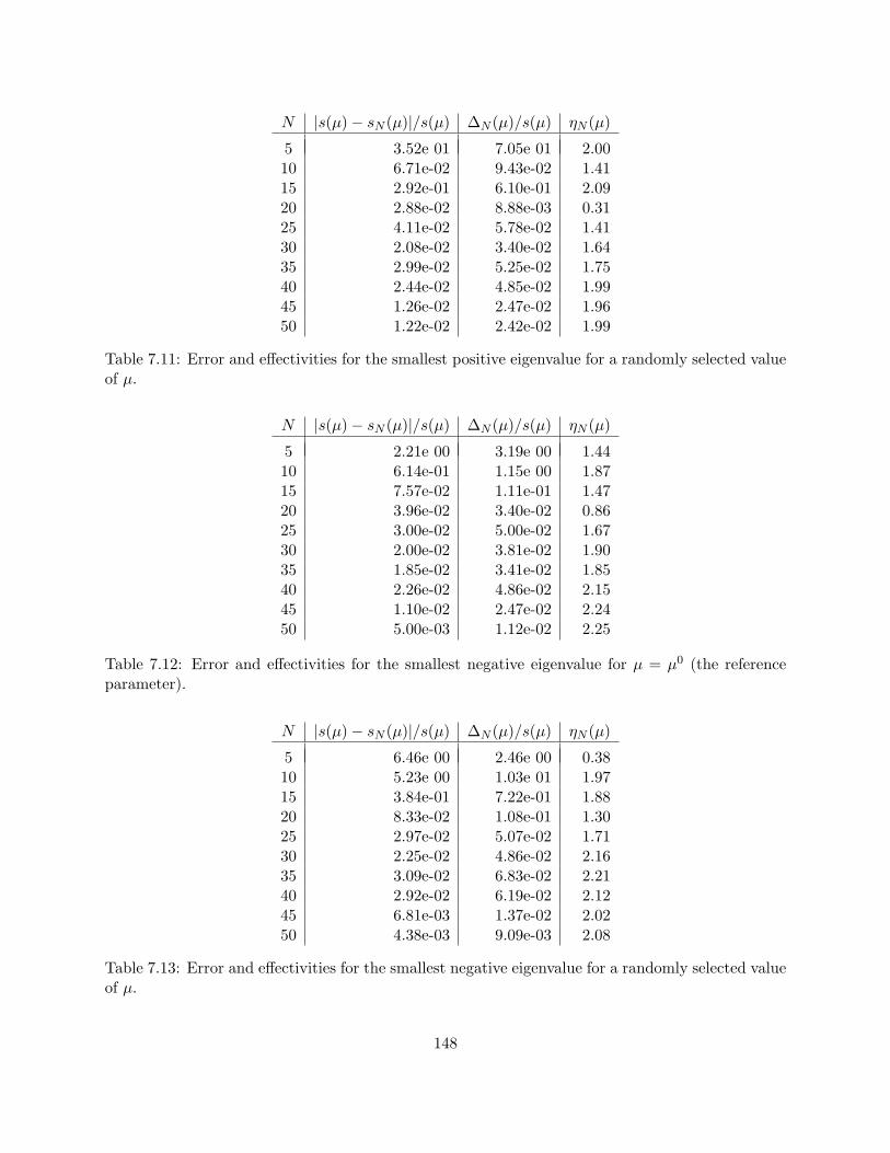
N |s(µ)− sN (µ)|/s(µ) ∆N (µ)/s(µ) ηN (µ)

5 3.52e 01 7.05e 01 2.0010 6.71e-02 9.43e-02 1.4115 2.92e-01 6.10e-01 2.0920 2.88e-02 8.88e-03 0.3125 4.11e-02 5.78e-02 1.4130 2.08e-02 3.40e-02 1.6435 2.99e-02 5.25e-02 1.7540 2.44e-02 4.85e-02 1.9945 1.26e-02 2.47e-02 1.9650 1.22e-02 2.42e-02 1.99

Table 7.11: Error and effectivities for the smallest positive eigenvalue for a randomly selected valueof µ.

N |s(µ)− sN (µ)|/s(µ) ∆N (µ)/s(µ) ηN (µ)

5 2.21e 00 3.19e 00 1.4410 6.14e-01 1.15e 00 1.8715 7.57e-02 1.11e-01 1.4720 3.96e-02 3.40e-02 0.8625 3.00e-02 5.00e-02 1.6730 2.00e-02 3.81e-02 1.9035 1.85e-02 3.41e-02 1.8540 2.26e-02 4.86e-02 2.1545 1.10e-02 2.47e-02 2.2450 5.00e-03 1.12e-02 2.25

Table 7.12: Error and effectivities for the smallest negative eigenvalue for µ = µ0 (the referenceparameter).

N |s(µ)− sN (µ)|/s(µ) ∆N (µ)/s(µ) ηN (µ)

5 6.46e 00 2.46e 00 0.3810 5.23e 00 1.03e 01 1.9715 3.84e-01 7.22e-01 1.8820 8.33e-02 1.08e-01 1.3025 2.97e-02 5.07e-02 1.7130 2.25e-02 4.86e-02 2.1635 3.09e-02 6.83e-02 2.2140 2.92e-02 6.19e-02 2.1245 6.81e-03 1.37e-02 2.0250 4.38e-03 9.09e-03 2.08

Table 7.13: Error and effectivities for the smallest negative eigenvalue for a randomly selected valueof µ.

148

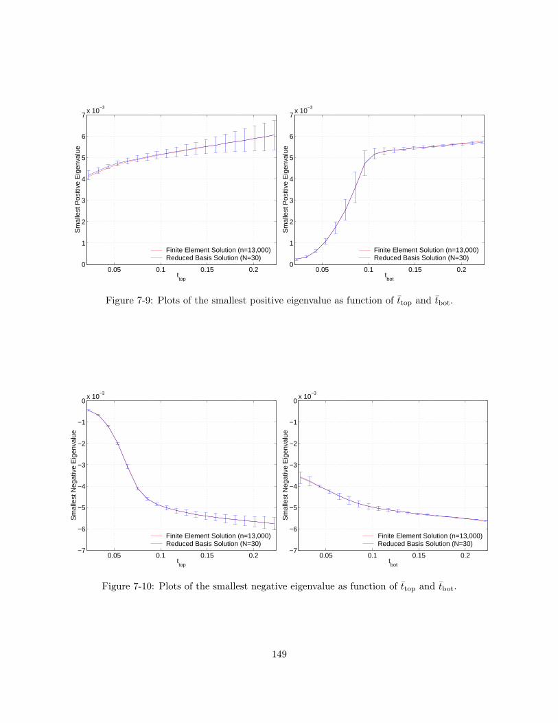
0.05 0.1 0.15 0.20

1

2

3

4

5

6

7x 10

−3

ttop

Sm

alle

st P

ositi

ve E

igen

valu

e

Finite Element Solution (n=13,000)Reduced Basis Solution (N=30)

0.05 0.1 0.15 0.20

1

2

3

4

5

6

7x 10

−3

tbot

Sm

alle

st P

ositi

ve E

igen

valu

e

Finite Element Solution (n=13,000)Reduced Basis Solution (N=30)

Figure 7-9: Plots of the smallest positive eigenvalue as function of ttop and tbot.

0.05 0.1 0.15 0.2−7

−6

−5

−4

−3

−2

−1

0x 10

−3

ttop

Sm

alle

st N

egat

ive

Eig

enva

lue

Finite Element Solution (n=13,000)Reduced Basis Solution (N=30)

0.05 0.1 0.15 0.2−7

−6

−5

−4

−3

−2

−1

0x 10

−3

tbot

Sm

alle

st N

egat

ive

Eig

enva

lue

Finite Element Solution (n=13,000)Reduced Basis Solution (N=30)

Figure 7-10: Plots of the smallest negative eigenvalue as function of ttop and tbot.

149

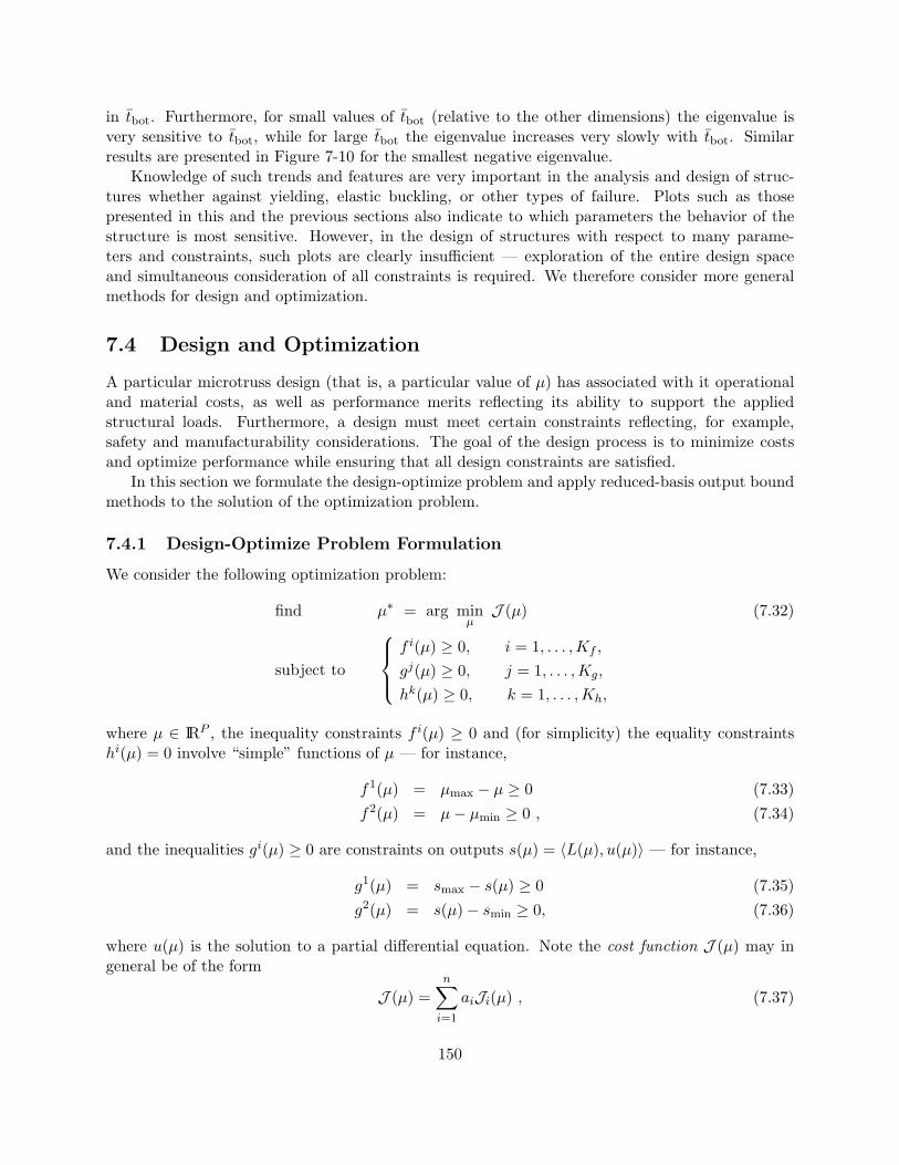
in tbot. Furthermore, for small values of tbot (relative to the other dimensions) the eigenvalue isvery sensitive to tbot, while for large tbot the eigenvalue increases very slowly with tbot. Similarresults are presented in Figure 7-10 for the smallest negative eigenvalue.

Knowledge of such trends and features are very important in the analysis and design of struc-tures whether against yielding, elastic buckling, or other types of failure. Plots such as thosepresented in this and the previous sections also indicate to which parameters the behavior of thestructure is most sensitive. However, in the design of structures with respect to many parame-ters and constraints, such plots are clearly insufficient — exploration of the entire design spaceand simultaneous consideration of all constraints is required. We therefore consider more generalmethods for design and optimization.

7.4 Design and Optimization

A particular microtruss design (that is, a particular value of µ) has associated with it operationaland material costs, as well as performance merits reflecting its ability to support the appliedstructural loads. Furthermore, a design must meet certain constraints reflecting, for example,safety and manufacturability considerations. The goal of the design process is to minimize costsand optimize performance while ensuring that all design constraints are satisfied.

In this section we formulate the design-optimize problem and apply reduced-basis output boundmethods to the solution of the optimization problem.

7.4.1 Design-Optimize Problem Formulation

We consider the following optimization problem:

find µ∗ = arg minµ

J (µ) (7.32)

subject to

f i(µ) ≥ 0, i = 1, . . . ,Kf ,

gj(µ) ≥ 0, j = 1, . . . ,Kg,

hk(µ) ≥ 0, k = 1, . . . ,Kh,

where µ ∈ IRP , the inequality constraints f i(µ) ≥ 0 and (for simplicity) the equality constraintshi(µ) = 0 involve “simple” functions of µ — for instance,

f1(µ) = µmax − µ ≥ 0 (7.33)f2(µ) = µ− µmin ≥ 0 , (7.34)

and the inequalities gi(µ) ≥ 0 are constraints on outputs s(µ) = 〈L(µ), u(µ)〉 — for instance,

g1(µ) = smax − s(µ) ≥ 0 (7.35)g2(µ) = s(µ)− smin ≥ 0, (7.36)

where u(µ) is the solution to a partial differential equation. Note the cost function J (µ) may ingeneral be of the form

J (µ) =n∑

i=1

aiJi(µ) , (7.37)

150

where the ai are weights and the Ji are different cost metrics.

Microtruss Design-Optimize Problem

We now consider a particular instantiation of our abstract optimization formulation. We considerhere a simpler version of the optimization problem posed in Chapter 1 involving only outputs relatedto the structural aspects of the problem; the full multifunctional (thermo-structural) problem isaddressed in [33].

As indicated in Chapter 1, one of the main advantages of the truss design is that it offersrelatively high structural load capacities at low weights, making it useful for weight-sensitive ap-plications such as next-generation rocket engines and unmanned autonomous vehicles (UAVs).Furthermore, the weight of the structure is directly related to the amount of material utilized,which in turn is related to material costs; in the case of rocket engines and UAVs, the weight isalso directly related to fuel consumption (operational costs). We may thus define our cost functionto be the area of the structure, J (µ) = V(µ), where µ = ttop, tbot, t, α, and

V(µ) = 2[(tt + tb)

(H

tanα+

t

sin α+ tb

)+ H

(t

sinα+ tb

)]. (7.38)

Furthermore, we require that (i) the parameter µ be in the design set, i.e., µ ∈ Dµ ⊂ IRP , whereDµ = [0.022, 0.22]3 × [0, 45], (ii) the length of the structure be equal to `0,

`(µ) = 2(

H

tanα+

t

sin α+ tb

)= `0 ; (7.39)

(iii) the deflection be less than a prescribed limit,

δave(µ) ≤ α1δmax, (7.40)

and (iv) the average stress near the support be less than the yield stress,

σave(µ) ≤ α2σY ; (7.41)

for this simpler formulation we shall not consider stability (buckling).

151

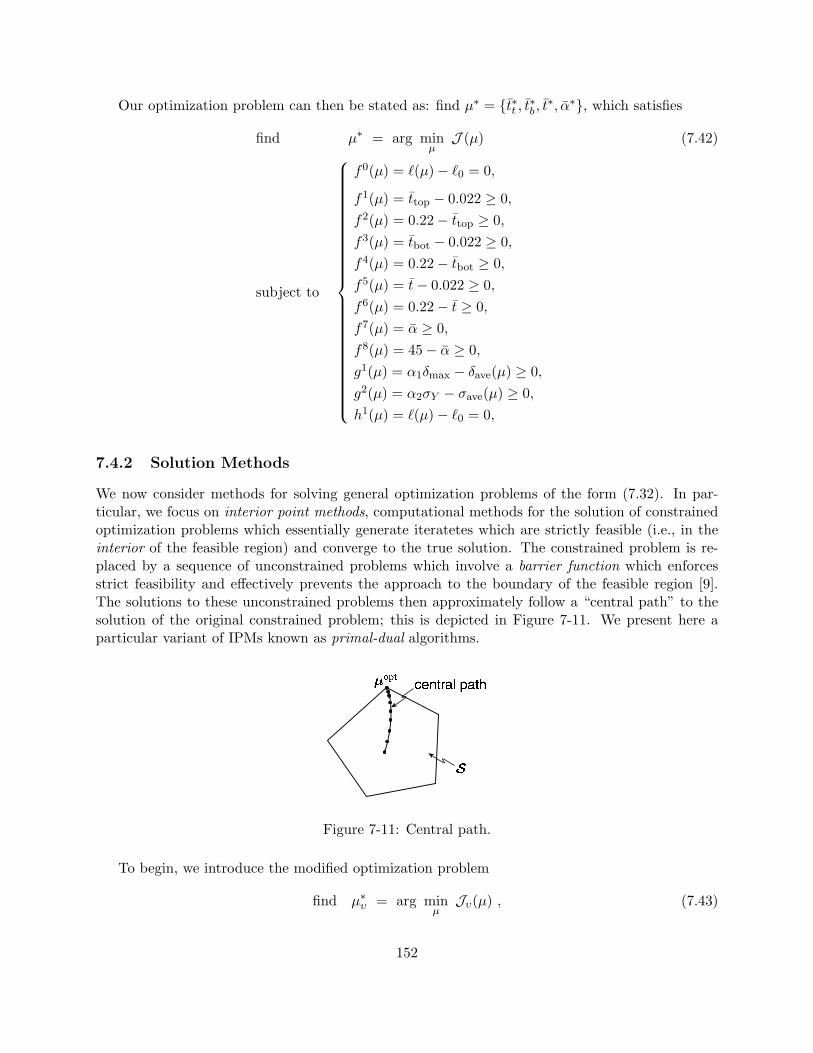
Our optimization problem can then be stated as: find µ∗ = t∗t , t∗b , t∗, α∗, which satisfies

find µ∗ = arg minµ

J (µ) (7.42)

subject to

f0(µ) = `(µ)− `0 = 0,

f1(µ) = ttop − 0.022 ≥ 0,f2(µ) = 0.22− ttop ≥ 0,f3(µ) = tbot − 0.022 ≥ 0,f4(µ) = 0.22− tbot ≥ 0,f5(µ) = t− 0.022 ≥ 0,f6(µ) = 0.22− t ≥ 0,f7(µ) = α ≥ 0,f8(µ) = 45− α ≥ 0,g1(µ) = α1δmax − δave(µ) ≥ 0,g2(µ) = α2σY − σave(µ) ≥ 0,h1(µ) = `(µ)− `0 = 0,

7.4.2 Solution Methods

We now consider methods for solving general optimization problems of the form (7.32). In par-ticular, we focus on interior point methods, computational methods for the solution of constrainedoptimization problems which essentially generate iteratetes which are strictly feasible (i.e., in theinterior of the feasible region) and converge to the true solution. The constrained problem is re-placed by a sequence of unconstrained problems which involve a barrier function which enforcesstrict feasibility and effectively prevents the approach to the boundary of the feasible region [9].The solutions to these unconstrained problems then approximately follow a “central path” to thesolution of the original constrained problem; this is depicted in Figure 7-11. We present here aparticular variant of IPMs known as primal-dual algorithms.

Figure 7-11: Central path.

To begin, we introduce the modified optimization problem

find µ∗υ = arg minµ

Jυ(µ) , (7.43)

152

where the modified cost functional is given by

Jυ(µ) ≡ J (µ)− υb

Kf∑i=1

ln fi(µ) +Kg∑j=1

ln gj(µ)

+1

2υp

Kh∑k=1

hk(µ)2; (7.44)

it can then be shown [15] that as υ = (υb, υp) → 0, the solution to (7.43) approaches the solutionto the original constrained optimization problem (7.32) — that is,

µ∗ = limυ→0

µ∗υ . (7.45)

We therefore wish to find µ∗υ such that

∇Jυ(µ∗υ) = ∇µJ(µ∗υ)− υb

Kf∑i=1

∇µfi(µ∗υ)fi(µ∗υ)

+Kg∑j=1

∇µgj(µ∗υ)gj(µ∗υ)

+1υp

Kh∑k=1

hk(µ)∇µhk(µ) = 0 (7.46)

in the limit as υ → 0.

We now introduce the “slack” variables F ∈ IRKh and G ∈ IRKg given by

F i =υ

fi(µ), i = 1, . . . ,Kf , (7.47)

Gi =υ

gi(µ), i = 1, . . . ,Kg, (7.48)

and define z = (µ, F,G) and

F(z; υ) =

∇µJ (µ) +Kf∑i=1

F i∇µfi(µ) +Kg∑i=1

Gi∇µgi(µ) +1υp

Kh∑i=1

hi(µ)∇µhi(µ)

F1f1(µ)− υ

...

FKffKf

(µ)− υ

G1g1(µ)− υ

...

GKggKg(µ)− υ

. (7.49)

The optimizer z∗ = (µ∗, F ∗, G∗) then satisfies

F(z∗; υ) = 0, as υ → 0. (7.50)

Applying Newton’s method to (7.50) and letting υ → 0, the primal-dual interior point algorithmmay thus be summarized as follows:

153

Set υ > 0, 0 < ε < 1for i = 1,. . . ,max iter do

while ||F (z; υ)|| > tol do∆z = [∇zF (z; υ)]−1 F (z);

Set γ = min

1, 0.95 mini

zi−∆zi

;

z = z + γ∆z;end whileυ = ευ

end for.

Note the factor γ is chosen such that the iterate z + γ∆z is strictly in the interior of the feasibleset.

Clearly, solution of the full optimization problem is computationally very expensive since itrequires repeated evaluation for many different values of the parameter µ of the outputs of interest.However, this is precisely the type of situation in which reduced-basis methods are most useful; wetherefore pursue a reduced-basis approach.

7.4.3 Reduced-Basis Approach

To begin, we again consider the optimization problem (7.32) but replace gi(µ) with the “appropri-ate” reduced-basis approximation such that feasibility is guaranteed,

find µ∗N = arg minµ

J (µ) (7.51)

subject to

f i(µ) ≥ 0, i = 1, . . . ,Kf ,

giN (µ) ≥ 0, i = 1, . . . ,Kg.

For example, in place of the gi(µ) defined in (7.35)-(7.36) we would take

g1N (µ) = smax − s+N (µ), (7.52)g2N (µ) = s−N (µ)− smin . (7.53)

Note if s−N (µ) ≤ s(µ) ≤ s+N (µ), and if the gN (µ) are appropriately defined (as in (7.52)-(7.53)), thesolution µ∗N to (7.51) is guaranteed to be feasible in the sense of (7.32)

The advantage of using reduced-basis methods in solving our optimization problem is twofold:(i) the low computational cost of evaluating (online) the outputs of interest allow for fast andefficient solution of the optimization problem; and (ii) rigorous error estimators and output boundsguarantee feasibility of the solution obtained from (7.51).

7.4.4 Results

We present in Table 7.14 the results of our optimization procedure for several scenarios. For thisexample we take the yield stress to be 30MPa, and the maximum deflection to be 0.03mm. Notethat in this case the angle effectively serves only to ensure that the equality constraint `(µ) = `0(µ)is satisfied. In Scenario 1, we obtain an initial guess which satisfies all the constraints but is not

154

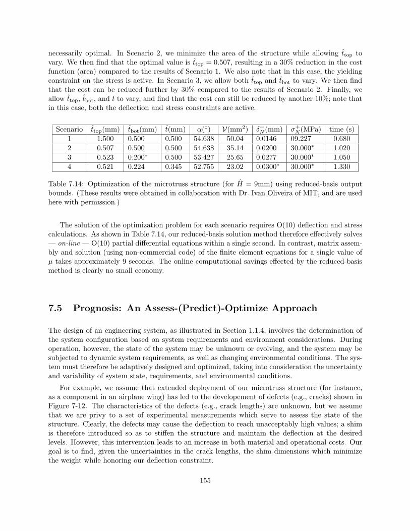
necessarily optimal. In Scenario 2, we minimize the area of the structure while allowing ttop tovary. We then find that the optimal value is ttop = 0.507, resulting in a 30% reduction in the costfunction (area) compared to the results of Scenario 1. We also note that in this case, the yieldingconstraint on the stress is active. In Scenario 3, we allow both ttop and tbot to vary. We then findthat the cost can be reduced further by 30% compared to the results of Scenario 2. Finally, weallow ttop, tbot, and t to vary, and find that the cost can still be reduced by another 10%; note thatin this case, both the deflection and stress constraints are active.

Scenario ttop(mm) tbot(mm) t(mm) α() V(mm2) δ+N (mm) σ+N (MPa) time (s)

1 1.500 0.500 0.500 54.638 50.04 0.0146 09.227 0.6802 0.507 0.500 0.500 54.638 35.14 0.0200 30.000∗ 1.0203 0.523 0.200∗ 0.500 53.427 25.65 0.0277 30.000∗ 1.0504 0.521 0.224 0.345 52.755 23.02 0.0300∗ 30.000∗ 1.330

Table 7.14: Optimization of the microtruss structure (for H = 9mm) using reduced-basis outputbounds. (These results were obtained in collaboration with Dr. Ivan Oliveira of MIT, and are usedhere with permission.)

The solution of the optimization problem for each scenario requires O(10) deflection and stresscalculations. As shown in Table 7.14, our reduced-basis solution method therefore effectively solves— on-line — O(10) partial differential equations within a single second. In contrast, matrix assem-bly and solution (using non-commercial code) of the finite element equations for a single value ofµ takes approximately 9 seconds. The online computational savings effected by the reduced-basismethod is clearly no small economy.

7.5 Prognosis: An Assess-(Predict)-Optimize Approach

The design of an engineering system, as illustrated in Section 1.1.4, involves the determination ofthe system configuration based on system requirements and environment considerations. Duringoperation, however, the state of the system may be unknown or evolving, and the system may besubjected to dynamic system requirements, as well as changing environmental conditions. The sys-tem must therefore be adaptively designed and optimized, taking into consideration the uncertaintyand variability of system state, requirements, and environmental conditions.

For example, we assume that extended deployment of our microtruss structure (for instance,as a component in an airplane wing) has led to the developement of defects (e.g., cracks) shown inFigure 7-12. The characteristics of the defects (e.g., crack lengths) are unknown, but we assumethat we are privy to a set of experimental measurements which serve to assess the state of thestructure. Clearly, the defects may cause the deflection to reach unacceptably high values; a shimis therefore introduced so as to stiffen the structure and maintain the deflection at the desiredlevels. However, this intervention leads to an increase in both material and operational costs. Ourgoal is to find, given the uncertainties in the crack lengths, the shim dimensions which minimizethe weight while honoring our deflection constraint.

155

ΓD

ΓtN

ft

Figure 7-12: A “defective” microtruss structure. The insert highlights the defects (two cracks) andintervention (shim).

L1 L2

tshim

Lshim

Figure 7-13: Parameters describing the defects, (L1 and L2), and the intervention, (Lshim andtshim).

156

7.5.1 Assess-Optimize Problem Formulation

More precisely, we characterize our system with a multiparameter µ = (µcrack, µshim) where µcrack =(L1, L2) and µshim = (Lshim, tshim). As shown in Figure 1-5, L1 and L2 are our “current guesses”for the relative lengths of the cracks on the upper frame and truss, respectively, while tshim andLshim denote the thickness and length of the shim, respectively; we also denote by µ∗crack = (L∗1, L

∗2)

the (real) unknown crack lengths. We further assume we are given Mexp intervals [δmLB, δ

mUB],

m = 1, . . . ,Mexp representing experimental measurements of the deflection such that

δave(µmshim, µ

∗crack) ∈ [δm

LB, δmUB], m = 1, . . . ,Mexp . (7.54)

From these measurements, we then infer the existence of a set L∗ such that (L∗1, L∗2) ∈ L∗. We then

wish to find the µ∗shim which satisfies

µ∗shim = arg minµshim

Vshim(µshim), (7.55)

where Vshim(µshim) = tshimLshim is simply the area of the shim, such that

µshim ∈ Dshim (7.56)max

µcrack∈L∗δave(µshim, µcrack) ≤ δmax . (7.57)

In words, we wish to find the shim dimensions which minimizes the area of the shim such thatthe maximum deflection (over all crack lengths consistent with the experiments) is less than theprescribed deflection limit δmax.

7.5.2 Solution Methods

Unfortunately, the set L∗ is very costly to construct. However, we can readily calculate a conser-vative approximation to L∗, L∗, by (i) applying our sharp yet computationally inexpensive outputbounds, and (ii) exploiting the readily proven monotonicity (increasing) property of δ(µ) withrespect to L1 and L2.

By construction, the surrogate L∗ contains L∗; we may thus replace (7.55) by:

µ∗shim = arg minµshim∈Dshim

Vshim(µshim) (7.58)

s.t. maxµcrack∈L∗

δ(µshim, µcrack) ≤ δmax,

since if µ∗shim satisfies maxµcrack∈L∗ δ(µcrack, µ∗shim) ≤ δmax then it follows that maxµcrack∈L∗ δ(µcrack, µ

∗shim) ≤

δmax. By once again exploiting the monotonicity of δ(µ) with respect to µcrack, we can readily findthe maximizer of δ over L∗; to wit, we define

µ′crack = arg maxµcrack∈L∗

δ(µcrack, µshim),

where µ′crack (which is independent of µshim) is calculated by a simple binary chop or bisection

157

algorithm (see [2]). We may then write (7.58) as

µ∗shim = arg minµshim∈Dshim

Vshim(µshim) (7.59)

s.t. δ(µ′crack, µshim) ≤ δmax.

Finally, we again apply our sharp yet inexpensive a posteriori output bounds to arrive at

µ∗shim = arg minµshim∈Dshim

Vshim(µshim) (= Lshimtshim). (7.60)

s.t. δ+N (µ′crack, µshim) ≤ δmax.

The formulation (7.60) has several advantages. First, satisfaction of the constraints is guar-anteed: if δ+N (µ) ≥ δN (µ), and µ∗shim satisfies δ+N (µ′crack, µ

∗shim) ≤ δmax, then it follows that

δ(µ′crack, µ∗shim) ≤ δmax. Second, δ+N (µ) can be calculated efficiently: the online complexity to

calculate δ+N (µ) is only O(N3) — independent of the very high dimension of the truth finite el-ement space, N . Finally, the constrained minimization problem (7.60) is readily treated by theinterior point methods presented in Section 7.4.2.

We present in Table 7.15 the solution to the optimization problem (7.60) for several scenarios.The inputs to the algorithm are: the crack lengths (L∗1, L

∗2) ∈ [0.1, 0.75]2, which are “unknown”

(to the algorithm); the error in the measurements, ε ∈ [0.1, 5]%; and the upper bound on thedeflection, δmax, “typically” chosen to be between (say) 6400 and 6600. The outputs are: the upperbound δ+N (µ) and the shim volume Vshim(µshim) at optimality. We also present the computationtime required to solve the complete optimization problem.

As a first test case, we assume that after several missions our truss structure has developedcracks of lengths (L∗1, L

∗2) = (0.5, 0.5). The plane is immediately needed for a new mission which

requires δ(µ) ≤ δmax = 6600.0; a few crude deflection measurements (ε = 5.0%) are performed, fromwhich we conclude that a shim of (optimal) dimensions (L∗shim, t

∗shim) = (15.0, 0.84) (and volume

12.6) is required to ensure feasibility.Next, we assume that for the next mission, the constraint on the deflection is now tighter,

δmax = 6400.0; (L∗1, L∗2, and ε are unchanged.) Measurement and optimization confirm that, as

anticipated, a larger shim with a volume of 20.9 is needed, with (L∗shim, t∗shim) = (15.0, , 1.4). When

the plane returns, more accurate measurements (ε = 0.1%) can now be afforded. (We assume thatL∗1, L

∗2, and δmax are unchanged.) On the basis of these new measurements, it is found that a shim

of volume 8.5 and dimensions (15.0, 0.57) actually suffices.After a subsequent mission, we assume that the crack length L∗2 has increased to 0.7. Upon

taking new measurements (ε = 0.1%), it is found that for the same deflection limit, δmax = 6400.0,an (optimal) shim of volume 8.62 and dimensions (L∗shim, t

∗shim) = (15.0, 0.57) is now required.

Next, we assume that the crack length L∗1 has increased to 0.7. New measurements and opti-mization reveal that a much bigger shim of volume 16.1 and dimensions (L∗shim, t

∗shim) = (15.0, 1.1)

is now required. The analysis automatically identifies these defects which most strongly affectperformance.

Lastly, we assume that, for a final mission, the constraint on the deflection can be relaxed,δmax = 6500.0. Measurement (ε = 0.1%) and optimization confirm that, as anticipated, a smallershim is sufficient, with volume 12.4 and (L∗shim, t

∗shim) = (15.0, 0.82).

We note that solution of a single optimization problem (for a given set of constraints) requiressolution of roughly 300 partial differential equations and associated sensitivity calculations (at

158

different parameter values).

L∗1 L∗2 ε(%) δmax δ+N (µ∗shim) Vshim(µ∗shim) Time(s)

0.5 0.5 5.0 6600 6600 12.6 9.40.5 0.5 5.0 6400 6400 20.9 7.10.5 0.5 0.1 6400 6400 8.5 7.60.5 0.7 0.1 6400 6400 8.6 7.50.7 0.7 0.1 6400 6400 16.1 9.50.7 0.7 0.1 6500 6500 12.4 10.1

Table 7.15: Solution to the assess-optimize problem with evolving (unknown) system characteristicsand varying constraints.

159

160

Chapter 8

Summary and Future Work

8.1 Summary

The main goal of this thesis is to develop reduced-basis methods for problems in elasticity. Theessential components are (i) rapidly convergent global reduced-basis approximations — projectiononto a space WN spanned by solutions of the governing partial differential equation at N selectedpoints in parameter space; (ii) a posteriori error estimation — relaxations of the error-residualequation that provide inexpensive bounds for the error in the outputs of interest; and (iii) off-line/on-line computational procedures — methods which decouple the generation and projectionstages of the approximation process. The operation count for the on-line stage — in which, givena new parameter value, we calculate the output of interest and associated error bound — dependsonly on N (typically very small) and the parametric complexity of the problem; the method isthus ideally suited for the repeated and rapid evaluations required in the context of parameterestimation, design, optimization, and real-time control.

Perhaps the biggest challenge in applying reduced-basis output bound methods to problems inlinear elasticity lies in developing rigorous (Method I) and inexpensive a posteriori error estimators.The need for rigorous output bounds is clear: in many real-world applications, certifiability ofapproximations is required so as to rigorously satisfy the prescribed application constraints.

In this thesis, we find that our Method I a posteriori error estimation procedures rely criticallyon the existence of a “bound conditioner” — in essence, an operator preconditioner that (i) satis-fies an additional spectral “bound” requirement, and (ii) admits the reduced-basis off-line/on-linecomputational stratagem. This improved understanding of reduced-basis a posteriori error estima-tion allows us to develop new techniques — in fact, recipes — for constructing the required boundconditioners.

To investigate the effectivity of these bound conditioner constructions, we first apply them inChapter 4 to the problem of heat conduction, and in Chapter 5 to the problem of linear elasticity.Problems in heat conduction serve as a good test bed for our methods prior to application tolinear elasticity: the Laplace operator is a “simpler version” of the linear elasticity operator. Thesetheoretical and numerical tests show that our bound conditioners perform remarkably well — weachieve good effectivities, and therefore sharp output bounds; and enable a better understandingof the strengths and limitations of each of technique.

Although some of our Method I techniques have been found to be generally applicable, in somecases — particularly for linear elasticity — the computational cost is still relatively high, and the

161

implementation difficult. We therefore also develop Method II error estimators — bounds whichare simple and inexpensive, albeit at the loss of complete certainty. Nevertheless, numerical testsshow that these simple bounds perform quite well.

There are also many applications in which the posibility of unstable equilibria must be con-sidered. While analytical formulas exist for the critical loads of relatively simple geometries, theyare of limited applicability particularly for more complex structures. However, exact (finite ele-ment) solution of the partial differential equations governing elastic stability is computationallytoo expensive, especially in the “many queries” context of design and optimization. We thereforeconsider in Chapter 6 reduced-basis approximation and (Method II) error estimation methods forthe problem of elastic buckling.

Finally, in Chapter 7 we apply our reduced-basis approximation and (Method II) error esti-mation methods to the structural aspects of the microtruss example put forth in Chapter 1. Theadvantages of the reduced-basis method in the “many queries” context of optimization is clear: weachieve substantial computational economy as compared to conventional finite element solution.

It must be noted that there are still many aspects of reduced-basis methods which must stillbe investigated and improved, some of which are briefly discussed in Chapter 2. In this chapter wepresent two areas which are related to the methods and problems presented here. First, we considerthe problem of thermoelasticity, important for creating a full (linear) thermo-structural model ofthe microtruss example of Chapters 1 and 7. This problem is difficult due to the “propagation”of the reduced basis error: the temperature, which must also be approximated using reduced-basismethods, enters the linear elasticity equations as “data.” Second, we consider the Helmholtz or waveequation, important in nondestructive evaluation, structural health monitoring, and prognosis —contexts for which our Assess-Predict-Optimize methodology of Chapter 7 is relevant. This problemis difficult since the operator is no longer coercive. We present initial ideas for these problems inthe following sections.

8.2 Approximately Parametrized Data: Thermoelasticity

In this section we explore the situation in which the parametrized mathematical model is not ex-act. In particular, we permit error or imprecision in the data that define the linear functionalsin our problem. In the case of thermoelasticity, for instance, this error is introduced by reduced-basis approximation of the temperature which couples into the linear elasticity equations throughthe linear functional. The ideas presented here extend the methods put forth in [38] for approxi-mately parametrized operators to the simpler case in which the data (or loading) is approximately-parametrized; we develop these ideas for the particular case of thermoelasticity.

8.2.1 Formulation of the Thermoelasticity Problem

There are many important applications in which the changes in temperature may significantly affectthe deformation of a structure — the multifunctional microtruss structure of Chapters 1 and 7 isone example, as are sensors and actuators.

When an isotropic body is subjected to a temperature change T from the uniform referencestate temperature, it may develop thermal stresses such that the (linearized) stress-strain relations[29] become

σij = − Eαϑ

1− 2νδijT + Cijklεkl , (8.1)

162

where αϑ is the linear coefficient of thermal expansion, the strains εij are related to the deformationu by (5.8), Cijkl is the elasticity tensor, and the temperature T satisfies the partial differentialequation

〈AϑT , v〉 = 〈Fϑ, v〉 , ∀ v ∈ Yϑ . (8.2)

Here, Aϑ : Yϑ → Y ′ϑ and Fϑ ∈ Y ′

ϑ are given by (3.20) and (3.21), respectively. Note we assume thatαϑ is constant and the Cijkl independent of temperature change. Substituting (8.1) into (5.22), wefind that the deformation satisfies the partial differential equation

〈Au, v〉 = 〈F , v〉+ 〈HT , v〉 , ∀ v ∈ Y , (8.3)

where A : Y → Y ′ and F ∈ Y ′ are given by (5.24) and (5.25), respectively, and H is given by

〈H, v〉 =∫

Ω

Eαϑ

1− 2ν∂vi

∂xiT dΩ , ∀ v ∈ Y . (8.4)

Upon application of a continuous piecewise-affine transformation from Ω to a fixed (µ-independent)reference domain Ω we obtain from (8.2)

〈Aϑ(µ)ϑ(µ), v〉 = 〈Fϑ(µ), v〉 , ∀ v ∈ Yϑ , (8.5)

where Aϑ : Yϑ → Y ′ϑ and Fϑ ∈ Y ′

ϑ are given by (3.34) and (3.36), respectively; and (8.3)

〈A(µ)u(µ), v〉 = 〈F (µ), v〉+ 〈H(µ)ϑ(µ), v〉 , ∀ v ∈ Y , (8.6)

where A : Y → Y ′ and F ∈ Y ′ are given by (5.38) and (5.40), respectively. Here,

〈H(µ)ϑ(µ), v〉 =∫

Ωβij(µ)

∂vi

∂xjϑ(µ) dΩ , (8.7)

where

βij(µ) =Eαϑ

1− 2νGji (detG(µ))−1 . (8.8)

We note that H(µ) is affinely dependent on the parameter since

〈H(µ)w, v〉 =QH∑q=1

αqH〈H

qw, v〉 , (8.9)

where QH = d2, and for q(i, j) : 1, . . . , d2 → 1, . . . , QH,

αq(i,j)H (µ) = βij(µ) , 〈Hqw, v〉 =

∫Ω

∂vi

∂xjw dΩ ; (8.10)

we recall from Chapters 3 and 5 that Aϑ(µ), Fϑ(µ), A(µ), and F (µ) are also affine in the parameter.

163

8.2.2 Reduced-Basis Approximation

Temperature Approximation

As before, we sample our design space Dµ to create the parameter sample

SµM = µ1, . . . , µM ; (8.11)

we then introduce the reduced-basis approximation space for the temperature

W TM = spanφm = T (µm),m = 1, . . . ,M . (8.12)

Our reduced-order temperature approximation TM (µ) ∈W TM then satisfies

〈Aϑ(µ)TM (µ), v〉 = 〈Fϑ(µ), v〉 , ∀ v ∈W TM . (8.13)

Deformation Approximation

We now introduce a “model-truncated” problem: given µ ∈ Dµ, we find

s(µ) = 〈L(µ), u(µ)〉 , (8.14)

where u(µ) ∈ Y satisfies

〈A(µ)u(µ), v〉 = 〈F (µ), v〉+ 〈H(µ)ϑM (µ), v〉 , ∀ v ∈ Y . (8.15)

We again sample the parameter space to create

SµN = µ1, . . . , µN ; (8.16)

and introduce the reduced-basis approximation space for the deformation

W uN = spanζn = u(µn), n = 1, . . . , N . (8.17)

Our output approximation is then

sN (µ) = 〈L(µ), uN (µ)〉 , (8.18)

where uN (µ) ∈W uN satisfies

〈AuN (µ), v〉 = 〈F (µ), v〉+ 〈H(µ)ϑM (µ), v〉 , ∀ v ∈W uN . (8.19)

The offline/online computational procedure to find ϑM (µ), uN (µ), and sN (µ) is similar to thatdescribed in Chapters 3 and 5.

164

A Priori Theory

In this section, we find an a priori bound for |s(µ)− s(µ)|. By way of preliminaries, we shall supposethat any member w of the temperature space Yϑ may be expressed as

w =Q∑

q=1

wq

Qϕq (8.20)

where the ϕq are basis functions of Yϑ, and Q may be quite large. We may then write

ϑ(µ)− ϑM (µ) =Q∑

q=1

βq(µ)ϕq . (8.21)

Note that replacing (8.5) and (8.6) with a “truth approximation” defined over a finite element spaceYN of dimension N (as we do in actual practice) ensures that Q may be presumed finite withoutloss of generality; we may, for instance, take Q = N and the ϕq to be the finite element nodalbasis functions. (Recall that we assume YN is sufficiently rich such that uN , sN , uN , and sN areindistinguishable from u, s, u, and s.)

Following [38], we also introduce Q suitably regular open subdomains, Dq ⊂ Ω, 1 ≤ q ≤ Q,and assume that a given subdomain Dq intersects only finitely many other subdomains Dq′ (asQ → ∞). We next define parameter-independent inner products and norms over Dq, ((·, ·))q and||| · |||q ≡ ((·, ·))1/2

q , respectively. We assume that ||| · |||q is uniformly equivalent to || · ||H1(Dq) forall functions in H1(Dq) in the sense that the relevant constants may be bounded independent ofµ and Q. It then follows from our assumptions that there exists a positive finite constant ρΣ —independent of µ and Q — such that

Q∑q=1

|||v|Dq |||2q < (ρΣ)2||v||2Y , ∀ v ∈ Y . (8.22)

We now define

EL2(µ) =

Q∑q=1

β2q (µ)

∫Ωϕ2

q

1/2

, (8.23)

and require thatEL2(µ) ≤ E (8.24)

for E ∈ IR+ independent of µ and Q (and preferably small). We next define γq ∈ IR, 1 ≤ q ≤ Q, as

γq(µ) ≡supv∈Y

〈H(µ)ϕq, v〉|||v|Dq |||q(∫

Ωϕ2

q

)1/2, (8.25)

165

and require thatγmax

Q(µ) ≡ max

q∈1,...,Qγq(µ) ≤ γ , (8.26)

for γ independent of µ.

We can now show that

|s(µ)− s(µ)| ≤ ||L||Y ′

(C1 inf

vN∈W uN

||u(µ)− vN ||Y + C2 ρΣ E γ), ∀ µ ∈ Dµ (8.27)

where C1 and C2 depend only on coercivity and continuity constants.

To prove (8.27), we first introduce e(µ) = u(µ)− uN (µ), and further define e(µ) = u(µ)− uN (µ),and e(µ) = u(µ)− u(µ), such that e(µ) = e(µ) + e(µ). We can thus write

|s(µ)− sN (µ)| = |〈L(µ), e(µ)〉| (8.28)

=∣∣∣∣〈L, e(µ)〉||e(µ)||Y

||e(µ)||Y∣∣∣∣ (8.29)

≤ supv∈Y

〈L, v〉||v||Y

||e(µ) + e(µ)||Y (8.30)

≤ ||L||Y ′ (||e(µ)||Y + ||e(µ)||Y ) (8.31)

by the triangle inequality.

Furthermore, it immediately follows from standard Galerkin theory that

||e(µ)||Y ≤ C1 infv∈W u

N

||u(µ)− vN ||Y , (8.32)

where C1 depends only on the coercivity and continuity constants associated with A.

To bound ||e(µ)||Y , we note that

〈A(µ)e(µ), v〉 = 〈H(µ) (ϑ(µ)− ϑM (µ)) , v〉, ∀ v ∈ Y . (8.33)

166

Expanding ϑ(µ)− ϑM (µ), and choosing v = e(µ), we obtain

〈A(µ)e(µ), e(µ)〉 =Q∑

q=1

βq(µ)〈H(µ)φq, e(µ)〉 (8.34)

≤Q∑

q=1

|βq(µ)| 〈H(µ)ϕq, e(µ)〉||| e(µ)|Dq

|||q||| e(µ)|Dq

|||q (8.35)

≤Q∑

q=1

|βq(µ)|(∫

Ωϕ2

q

)1/2

supv∈Y

〈H(µ)ϕq, v〉||| v|Dq

|||q(∫Ωϕ2

q

)1/2

||| e(µ)|Dq|||q (8.36)

≤ γ

Q∑q=1

β2q (µ)

∫Ωϕ2

q

1/2 Q∑q=1

||| e(µ)|Dq|||2q

1/2

(8.37)

≤ γ E ρΣ ||e(µ)||Y . (8.38)

Finally, we have

C0A ≤ inf v ∈ Y 〈A(µ)v, v〉

||v||2Y(8.39)

≤ 〈A(µ)e(µ), e(µ)〉||e(µ)||2Y

, (8.40)

from which it follows that

〈A(µ)e(µ), e(µ)〉 ≤ C2 ρΣ E γ , ∀ µ ∈ Dµ , (8.41)

where C2 = 1/C0A.

The bound (8.27) then follows from (8.31), (8.32), and (8.41). Note that we can, in fact, improveour bound to be quadratic (and not linear) in ||e(µ)||Y by introduction of the reduced-basis adjointtechniques described in Chapter 5.

8.2.3 A Posteriori Error Estimation: Method I

We develop here the necessary a posteriori error bounds — a necessity for both efficiency andreliability.

Preliminaries

As in Chapters 4 and 5, we introduce a symmetric, coercive, continuous bound conditioner C(µ) : Y →Y ′ that satisfies the spectral condition

1 ≤ 〈A(µ)v, v〉〈C(µ)v, v〉

≤ ρ, ∀ v ∈ Y,∀ µ ∈ Dµ, (8.42)

167

for some preferably small constant ρ ∈ IR, as well as the computationally invertibility hypothesisC−1(µ) =

∑i∈I(µ) αi(µ)C−1

i . It then follows from the coercivity of C(µ) and our assumptions inSection 8.2.2 that there exists a bound ρ′Σ(µ) which is independent of Q, such that

Q∑q=1

|||v|Dq |||2q < (ρ′Σ(µ))2〈C(µ)v, v〉 , ∀ v ∈ Y . (8.43)

We also introduce a symmetric, coercive, continuous bound conditioner for the thermal problemCϑ(µ) : Yϑ → Y ′

ϑ that satisfies the (analogous) spectral and computational invertibility conditions.We then define

∆ϑM (µ) = 〈Rϑ(µ), C−1

ϑ (µ)Rϑ(µ)〉 (8.44)

where 〈Rϑ(µ), v〉 = 〈Aϑ(µ) (ϑ(µ)− ϑM (µ), v)〉 for all v ∈ Yϑ. From the results of Chapters 4 and5, it follows that the error in the reduced-basis approximation for the temperature in the energynorm is bounded by ∆ϑ

M (µ):

〈Aϑ(µ) (ϑ(µ)− ϑM (µ)) , (ϑ(µ)− ϑM (µ))〉 . (8.45)

We next define the operator D as

〈Dw, v〉 =Q∑

q=1

wq

Qvq

Q

∫Ωϕ2

q dΩ , ∀ w, v ∈ Yϑ , (8.46)

where the ϕq are the nodal basis functions and wq

Q, vq

Qthe nodal values of w, v, respectively; and

the eigenvalue λL2-H1

min (µ) as

λL2-H1

min (µ) = minv∈Yϑ

〈Cϑv, v〉〈Dv, v〉

; (8.47)

Furthermore, we have

supv∈Y

〈H(µ)ϕq, v〉|||v|Dq |||q

=QH∑k=1

αkH sup

v∈Y

〈Hkϕq, v〉|||v|Dq |||q

. (8.48)

Defining zqk ∈ Yq as

zqk = arg supv∈Y

〈Hkϕq, v〉|||v|Dq |||q

, (8.49)

it follows that((zqk, v|Dq)) = 〈Hkϕq, v〉, ∀ v ∈ Yq . (8.50)

168

We then have

supv∈Y

(〈H(µ)ϕq, v〉|||v|Dq |||q

)2

=

(QH∑k=1

αkH(µ)

〈Hkϕq, zqk〉|||zqk|||q

)2

(8.51)

=

(QH∑k=1

αkH((zqk, zqk))1/2

)2

(8.52)

=QH∑k=1

QH∑k′=1

αkHα

k′H((zqk, zqk))1/2((zqk′ , zqk′))1/2 (8.53)

= aϑ(µ)Zqa(µ) , (8.54)

where a(µ) ∈ IRQH and Zq ∈ IRQH×QH are given by

a(µ) =[α1H(µ) . . . αQH

H (µ)]T

(8.55)

andZq

kk′ = ((zqk, zqk))1/2((zqk′ , zqk′))1/2 . (8.56)

Finally, we let λZq

max be the maximum eigenvalue of Zq,

λZq

max = maxv∈IRQH

vTZqv

vT v(8.57)

and define

ΛZ = maxq∈1,...,Q

λZq

max∫Ωϕ2

q

(8.58)

Error Bound

Our error estimator for |s(µ)− sN (µ)| is then given by

∆N (µ) ≡ |||L|||Y ′

(δ(µ) + δ(µ)

), (8.59)

where

|||L|||Y ′ = supv∈Y

〈L(µ), v〉〈C(µ)v, v〉1/2

(8.60)

δ(µ) = 〈C(µ)E(µ), E(µ)〉1/2 (8.61)

δ(µ) =ρ′Σ∆ϑ

M (µ)ΛZ

(aT (µ)a(µ)

)1/2

λL2-H1

min (µ). (8.62)

169

Here E(µ) ∈ Y satisfies

〈C(µ)E(µ), v〉 = 〈H(µ) (ϑ(µ)− ϑM (µ)) , v〉, ∀ v ∈ Y . (8.63)

Clearly, δ(µ) measures the error due to the reduced-basis approximation of u(µ), and δ(µ) measuresthe error due to model truncation — the error due to the reduced-basis approximation of ϑ(µ) inthe data.

We now show that our estimator ∆N (µ) is, in fact, a rigorous upper bound for |s(µ)− sN (µ)|.To begin, we note that

|s(µ)− sN (µ)| = |〈L(µ), e(µ)〉| (8.64)

≤(

supv∈X

〈L(µ), v〉〈A(µ)v, v〉1/2

)〈A(µ)e(µ), e(µ)〉1/2 (8.65)

≤(

supv∈X

〈L(µ), v〉〈A(µ)v, v〉1/2

)(〈A(µ)e(µ), e(µ)〉1/2 + 〈A(µ)e(µ), e(µ)〉1/2

)(8.66)

We next note from the results of Chapters 4 and 5 that

〈A(µ)e(µ), e(µ)〉 ≤ 〈C(µ)E(µ), E(µ)〉 (8.67)

It follows that|s(µ)− sN (µ)| ≤ |||L|||Y ′

(δ(µ) + 〈A(µ)e(µ), e(µ)〉1/2

); (8.68)

it thus remains only to show that 〈A(µ)e(µ), e(µ)〉1/2 ≤ δ(µ).

We first define E(µ) ∈ Y as the solution to

〈C(µ)E(µ), v〉 = 〈H(µ) (ϑ(µ)− ϑM (µ)) , v〉, ∀ v ∈ Y ; (8.69)

it thus follows that〈A(µ)e(µ), e(µ)〉1/2 ≤ 〈C(µ)E(µ), E(µ)〉1/2 . (8.70)

170

We now note that

〈C(µ)E(µ), E(µ)〉 = 〈H(µ) (ϑ(µ)− ϑM (µ)) , E(µ)〉 (8.71)

≤Q∑

q=1

|βq(µ)| 〈H(µ)ϕq, E(µ)〉

||| E(µ)∣∣∣Dq

|||q|||E(µ)|Dq |||q (8.72)

≤Q∑

q=1

|βq(µ)|(∫

Ωϕ2

q

)1/2

supv∈Y

〈H(µ)ϕq, v〉|||v|Dq |||q(∫

Ωϕ2

q

)1/2

||| E(µ)∣∣∣Dq

|||q (8.73)

=Q∑

q=1

|βq(µ)|(∫

Ωϕ2

q

)1/2

γq(µ)||| E(µ)∣∣∣Dq

|||q (8.74)

≤ γmaxQ

(µ)

Q∑q=1

β2q (µ)

∫Ωϕ2

q

1/2 Q∑q=1

||| E(µ)∣∣∣Dq

|||2q

1/2

(8.75)

≤ γmaxQ

(µ)EL2(µ)ρ′Σ(µ) 〈C(µ)E(µ), E(µ)〉1/2 , (8.76)

and therefore〈C(µ)E(µ), E(µ)〉1/2 ≤ γmax

Q(µ)EL2(µ)ρ′Σ(µ) . (8.77)

From (8.21) and (8.46) we have

EL2(µ) =Q∑

q=1

β2q (µ)

∫Ωϕ2

q (8.78)

= 〈D (ϑ(µ)− ϑM (µ)) , (ϑ(µ)− ϑM (µ))〉1/2 (8.79)

≤

(supv∈Yϑ

〈Dv, v〉〈Aϑ(µ)v, v〉1/2

)〈Aϑ(µ) (ϑ(µ)− ϑM (µ)) , (ϑ(µ)− ϑM (µ))〉1/2 (8.80)

≤

(supv∈Yϑ

〈Dv, v〉〈Cϑ(µ)v, v〉1/2

)∆ϑ

M (µ) (8.81)

=∆ϑ

M (µ)λL2-H1

min

. (8.82)

171

We next note that(γmax

Q(µ))2

= maxq∈1,...,Q

(γq(µ))2 (8.83)

= maxq∈1,...,Q

aT (µ)Zqa(µ)∫Ωϕ2

q

(8.84)

= maxq∈1,...,Q

1∫Ωϕ2

q

(aT (µ)Zqa(µ)aT (µ)a(µ)

)aT (µ)a(µ) (8.85)

≤ aT (µ)a(µ) maxq∈1,...,Q

1∫Ωϕ2

q

maxv∈IRQH

vTZqv

vT v(8.86)

≤ aT (µ)a(µ) maxq∈1,...,Q

1∫Ωϕ2

q

λZq

max (8.87)

= aT (µ)a(µ)Λ2Z (8.88)

Finally, we have

〈A(µ)e(µ), e(µ)〉1/2 ≤ 〈C(µ)E(µ), E(µ)〉1/2 (8.89)

≤ρ′Σ(µ)∆ϑ

M (µ)ΛZ

(aT (µ)a(µ)

)1/2

λL2-H1

min

(8.90)

= δ(µ) . (8.91)

We note that λL2-H1

min and ΛZ can be calculated offline, while ∆ϑM (µ) and aT (µ) may be calculated

online.

8.3 Noncoercive Problems: The Reduced-Wave (Helmholtz) Equa-tion

There are many important problems for which the coercivity of A is lost — a representative exampleis the Helmholtz, or reduced–wave, equation. For noncoercive problems, well–posedness is nowensured only by the inf–sup condition. This “weaker” stability condition presents difficulties in bothapproximation and error estimation; we shall address the latter in this section. In particular, wepresent some preliminary ideas for constructing approximations to the inf-sup parameter βA(µ) for(i) noncoercive problems in general, through application of certain bound conditioner constructionspresented in Chapter 3; and (ii) the Helmholtz problem in particular, through ...

8.3.1 Abstract Formulation

We again consider a suitably regular (smooth) domain Ω ⊂ IRd, d = 1, 2, or 3, and associatedfunction space Y ⊂ (H1(Ω))p with associated inner product and norm (·, ·)Y and || · ||Y = (·, ·)1/2

Y ,respectively. We recall that the dual space of Y , Y ′, is defined as the set of all linear functionals F

172

such that the dual norm of F , defined as ||F ||Y ′ ,

||F ||Y ′ = supv∈Y

〈F, v〉||v||Y

, (8.92)

is bounded.We then consider the problem: for any µ ∈ Dµ, find s(µ) = 〈L(µ), u(µ)〉 where u(µ) satisfies

〈A(µ)u(µ), v〉 = 〈F (µ), v〉, ∀ v ∈ Y , (8.93)

where the operator A(µ) : Y → Y ′ is symmetric, 〈A(µ)w, v〉 = 〈A(µ)v, w〉, continuous,

〈A(µ)w, v〉 ≤ γA(µ)||w||Y ||v||Y ≤ γ0A||w||Y ||v||Y , ∀ w, v ∈ Y, ∀ µ ∈ Dµ , (8.94)

and depends affinely on the parameter

A(µ) =QA∑q=1

Θq(µ)Aq; (8.95)

we further assume that F (µ) ∈ Y ′, L(µ) ∈ Y ′, and that F , L also depend affinely on the µ. Inaddition to the primal problem (8.93), we shall again require the dual problem

〈A(µ)v, ψ(µ)〉 = 〈L(µ), v〉, ∀ v ∈ Y , (8.96)

where ψ(µ) ∈ Y .In this section, we no longer assume that A(µ) is coercive, but instead ensure well-posedness

by the inf-sup stability condition

0 < β0A ≤ βA(µ) = inf

w∈Ysupv∈Y

〈A(µ)w, v〉||w||Y ||v||Y

, ∀ µ ∈ Dµ ; (8.97)

Several numerical difficulties arise due to this “weaker” stability condition. The first difficulty ispreservation of the inf-sup stability condition for finite dimensional approximation spaces. Althoughin the coercive case restriction to the space WN actually increases stability, in the noncoercive caserestriction to the space WN can easily decrease stability: the relevant supremizers may not beadequately represented. Furthermore, loss of stability can lead to poor approximations — the inf-sup parameter enters in the denominator of the a priori convergence result (3.92). Nevertheless,it is posssible to resolve these issues by considering projections other than standard Galerkin, and“enriched” approximation spaces [26, 43]. The second numerical difficulty — which we shall addresshere — is estimation of the inf-sup parameter βA(µ), important for certain classes of Method I aposteriori techniques. Since βA(µ) can not typically be deduced analytically, it must therefore beapproximated. To motivate our methods, we first consider an example.

8.3.2 Formulation of the Helmholtz Problem

There are many important applications in which the Helmholtz equation takes a central role —nondestructive evaluation, structural dynamics, and electromagnetics, for example.

We consider an isotropic body subjected to a harmonic loading such that the harmonic response

173

u is governed by the partial differential equation

∇2u+ ω2u = b, in Ω , (8.98)

with boundary conditions

u = 0 on ΓD (8.99)∂u

∂xjenj = f on ΓN . (8.100)

Furthermore, we assume that the output of interest is a linear functional of the response,

s(µ) = 〈L(µ), u(µ)〉, for µ = ω ∈ Dµ . (8.101)

The problem may then be (weakly) formulated as: find s(µ) = 〈L(µ), u(µ)〉, where u(µ) ∈∈Y = v ∈ H1(Ω) | v = 0 on ΓD is the solution to

〈A(µ)u(µ), v〉 = 〈F (µ), v〉,∀ v ∈ Y ; (8.102)

for this example,

〈A(µ)w, v〉 =∫

Ω

∂v

∂xi

∂w

∂xidΩ + ω2

∫Ωw v dΩ , (8.103)

and〈F (µ), v〉 =

∫Ωb v dΩ +

∫Γfv dΓ . (8.104)

Affine parameter dependence of A(µ) is then obtained for QA = 2, and

Θ1(µ) = 1, 〈A1w, v〉 =∫

Ω

∂v

∂xi

∂w

∂xidΩ , (8.105)

Θ2(µ) = ω2, 〈A2w, v〉 =∫

Ωw v dΩ . (8.106)

8.3.3 Reduced-Basis Approximation and Error Estimation

Following [43], we assume that we have the reduced-basis approximations uN (µ) ∈WN and ψN (µ) ∈WN given by

uN (µ) = arg infw∈WN

supv∈VN

〈A(µ)(u(µ)− w), v〉||v||Y

, (8.107)

ψN (µ) = arg infw∈WN

supv∈VN

〈A(µ)v, (ψ(µ)− w)〉||v||Y

, (8.108)

where WN and VN are the appropriate infimizing and supremizing spaces, respectively. Our outputapproximation is then

sN (µ) = 〈L(µ), uN (µ)〉 , (8.109)

174

and the associated upper and lower bounds are s±N (µ) = sN (µ)±∆N (µ) where

∆N (µ) =1

βLBA (µ)

||Rpr(µ)||Y ′ ||Rdu(µ)||Y ′ , (8.110)

and0 < βLB

A (µ) ≤ βA(µ) ; (8.111)

we assume for the moment that a lower bound βLBA (µ) can be readily found.

We now show that ∆N (µ) is indeed an error bound, that is,

|s(µ)− sN (µ)| ≤ ∆N (µ) . (8.112)

To begin, we define Tµw as

Tµw = arg supv∈Y

〈A(µ)w, v〉||v||Y

; (8.113)

it then follows that Tµw satisfies

(Tµw, v)Y = 〈A(µ)w, v〉, ∀ v ∈ Y , (8.114)

and therefore

||Rpr(µ)||Y ′ = supv∈Y

〈Rpr(µ), v〉||v||Y

(8.115)

= supv∈Y

〈A(µ)(u(µ)− uN (µ)), v〉||v||Y

(8.116)

=〈A(µ)(u(µ)− uN (µ)), Tµ(u(µ)− uN (µ))〉

||Tµ(u(µ)− uN (µ))||Y(8.117)

=(Tµ(u(µ)− uN (µ)), Tµ(u(µ)− uN (µ)))Y

||Tµ(u(µ)− uN (µ))||Y(8.118)

= ||Tµ(u(µ)− uN (µ))||Y . (8.119)

Furthermore, we have

βA(µ)||ψ(µ)− ψN (µ)||Y ||Tµ(ψ(µ)− ψN (µ))||Y

≤ 〈A(µ)Tµ(ψ(µ)− ψN (µ)), (ψ(µ)− ψN (µ))〉 (8.120)

= 〈Rdu(µ), Tµ(ψ(µ)− ψN (µ))〉 (8.121)

=

∣∣〈Rdu(µ), Tµ(ψ(µ)− ψN (µ))〉∣∣

||Tµ(ψ(µ)− ψN (µ))||Y ′||Tµ(ψ(µ)− ψN (µ))||Y ′ (8.122)

≤ supv∈Y

〈Rdu(µ), v〉||v||Y ′

||Tµ(ψ(µ)− ψN (µ))||Y ′ (8.123)

= ||Rdu(µ)||Y ′ ||Tµ(ψ(µ)− ψN (µ))||Y ′ , (8.124)

175

and therefore||ψ(µ)− ψN (µ)||Y ≤ 1

βA(µ)||Rdu(µ)||Y ′ . (8.125)

Finally, we have

|s(µ)− sN (µ)| = |〈A(µ)(u(µ)− uN (µ)), (ψ(µ)− ψN (µ))〉| (8.126)

= |〈Rpr(µ), (ψ(µ)− ψN (µ))〉| (8.127)

=|〈Rpr(µ), (ψ(µ)− ψN (µ))〉|||Tµ(ψ(µ)− ψN (µ))||Y

||Tµ(ψ(µ)− ψN (µ))||Y (8.128)

≤ supv∈Y

〈Rpr(µ), v〉||v||Y ′

||ψ(µ)− ψN (µ)||Y (8.129)

= ||Rpr(µ)||Y ′ ||ψ(µ)− ψN (µ)||Y (8.130)

≤ 1βA(µ)

||Rpr(µ)||Y ′ ||Rdu(µ)||Y ′ (8.131)

≤ 1βLBA (µ)

||Rpr(µ)||Y ′ ||Rdu(µ)||Y ′ ; (8.132)

this completes the proof.

Approximation of the Stability Constant: Eigenvalue Interpolation

Since the stability constant βA(µ) can not typically be deduced analytically, an approximation —more precisely, a lower bound — must be calculated. We present here a method for calculating therequisite lower bound based on the the concave-eigenvalue interpolation methods of Chapter 4.

To begin, we assume that the inner product associated with the function space Y is given by

(w, v)Y ≡ 〈Cw, v〉 , (8.133)

where C : Y → Y ′ is a µ-independent, symmetric, continuous, and coercive operator; the associatednorm is then ||v||Y = 〈Cv, v〉1/2. It then follows from (8.114) that

〈C(Tµw), v〉 = 〈A(µ)w, v〉 , ∀ v ∈ Y , (8.134)

and therefore Tµw = C−1A(µ)w. We then note that

(βA(µ))2 = infw∈Y

〈A(µ)w, Tµw〉2

||w||2Y ||Tµw||2Y(8.135)

= infw∈Y

〈A(µ)w, Tµw〉 (Tµw, Tµw)Y

(w,w)Y (Tµw, Tµw)Y(8.136)

= infw∈Y

〈A(µ)w, C−1A(µ)w〉〈Cv, v〉

(8.137)

= infw∈Y

〈L(µ)w,w〉〈Cv, v〉

, (8.138)

176

whereL(µ) ≡ (C−1A(µ))TA(µ) = A(µ)C−1A(µ) . (8.139)

We also note from our assumption of affine parameter dependence (8.95) that L(µ) is also affinein µ since

L(µ) =

QA∑q=1

Θq(µ)Aq

C−1

QA∑q′=1

Θq′(µ)Aq′

(8.140)

=(Θ1(µ)

)2︸ ︷︷ ︸Φ1(µ)

[A1C−1A1

]︸ ︷︷ ︸

L1

+(2Θ1(µ)Θ2(µ)

)︸ ︷︷ ︸Φ2(µ)

[A1C−1A2

]︸ ︷︷ ︸

L2

+ · · · (8.141)

+(2ΘQA−1ΘQA

)︸ ︷︷ ︸ΦQL−1

[AQA−1C−1AQA

]︸ ︷︷ ︸

LQL−1

+(ΘQA

)2︸ ︷︷ ︸ΦQL

[AQA C−1AQA

]︸ ︷︷ ︸

LQL

(8.142)

≡QL∑q=1

Φq(µ)Lq , (8.143)

where QL = QA(QA + 1)/2. We now define

L(φ) ≡QL∑q=1

φq Lq (8.144)

where φ ∈ IRQL , L(φ) : Y → Y ′, and the Lq ≡ Lq are symmetric and continuous

〈Lqw, v〉 ≤ γLq(µ)||w||Y ||v||Y ≤ γ0Lq ||w||Y ||v||Y , ∀ w, v ∈ Y . (8.145)

We may then writeL(Φ(µ)) = L(µ) . (8.146)

It then follows that the stability constant βA(µ) is related to the eigenvalue problem

〈L(φ)ξ(φ), v〉 = λ(φ)〈Cξ(φ), v〉 (8.147)

In particular,βA(µ) = (λ1(Φ(µ)))1/2 , (8.148)

where λ1 is the smallest eigenvalue satisfying (8.120). Furthermore, we know from Chapter 4 thatλ1 is concave in φ. We can thus construct a lower bound λLB

1 (Φ(µ)) to λ1(Φ(µ)) as the convexcombination of λ1(φk):

λLB1 (Φ(µ)) =

∑k∈T (Φ(µ))

αkλ(φk) (8.149)

177

such that the αk > 0, and ∑k∈T (Φ(µ))

αk = 1 , (8.150)

∑k∈T (Φ(µ))

αkφk = Φ(µ) ; (8.151)

The problem of finding the best (largest) convex combination λLB1max(Φ(µ)) is again a linear program-

ming problem (which may or may not be feasible). Clearly, the choice βLBA (µ) = (λLB

1max(Φ(µ)))1/2

then satisfies (8.111).The potential difficulty with (8.149) is that the off-line stage may be expensive and also com-

plicated, and relatedly, that there is little a priori guidance (for the φk or T (Φ(µ))). Note inthis noncoercive case the relevant operator yields QL = O(Q2

A) coefficients, thus aggravating theproblems already identified in Chapter 4 — negative lower bounds, fine lookup tables, large Q.

178

Appendix A

Elementary Affine GeometricTransformations

We consider the case Ω(µ),Ω ⊂ IRd, d = 2; the extension to d = 1 and d = 3 is straightforward.

Stretch

We consider the mapping from Ω(µ) → Ω shown in Figure A-1(a) and A-1(f). The forward andinverse affine mappings are then given by (here, α is the angle of Ω(µ), and the angle of Ω is 0.)

G(µ) =

t1

t1(µ)·

· t2t2(µ)

, g(µ) = 0 , (A.1)

G−1(µ) =

t1(µ)t1

·

· t2(µ)t2

, g′(µ) = 0 . (A.2)

Horizontal Shear

We now consider the mapping from Ω(µ) → Ω shown in Figure A-1(b) and A-1(f). The forwardand inverse affine mappings are then given by

G(µ) =[

1 − tanα· 1

], g(µ) = 0 , (A.3)

G−1(µ) =[

1 tanα· 1

], g′(µ) = 0 . (A.4)

179

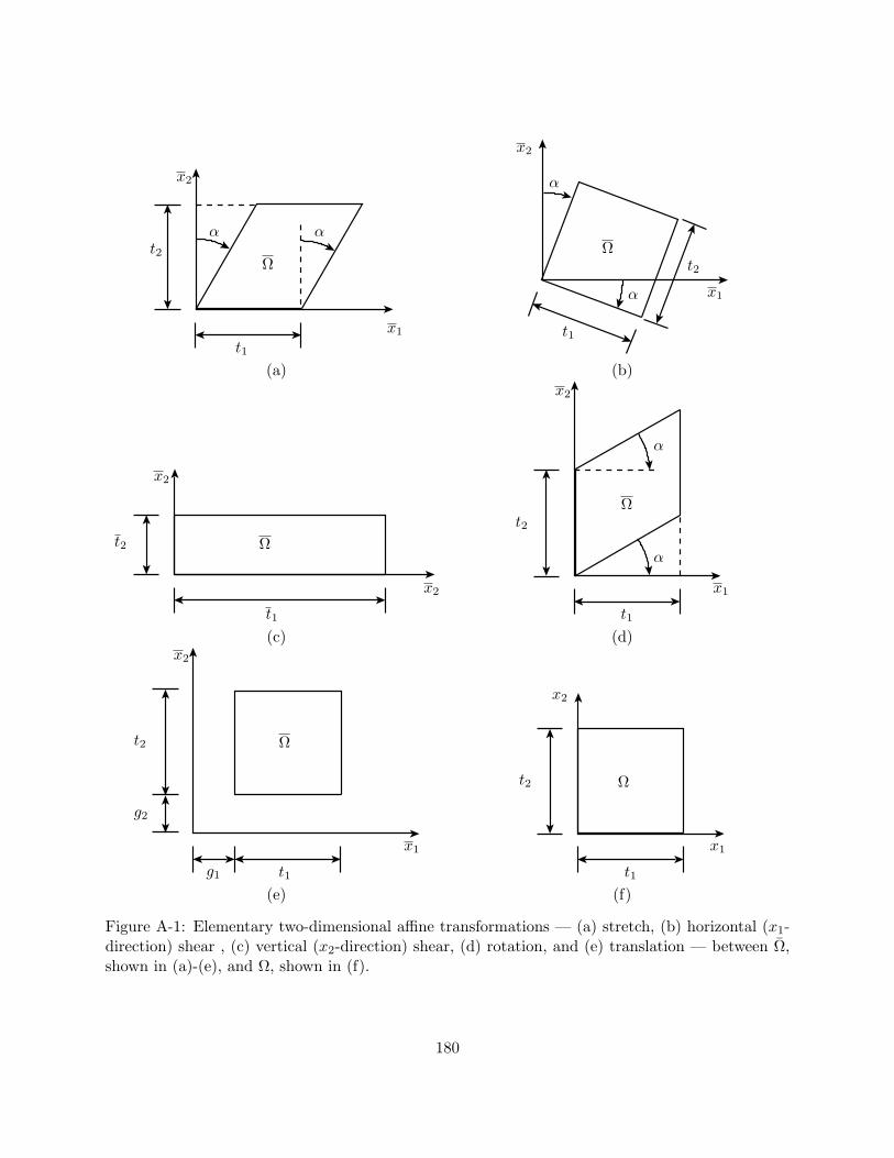
α α

x1

Ω

t1

x2

t2

(a)

x2

x1α

Ωt2

t1

α

(b)

x2

x2

t2

t1

Ω

(c)

α

α

Ω

x2

x1

t2

t1

(d)

Ω

x2

x1

g1 t1

g2

t2

(e)

x2

x1

Ωt2

t1

(f)

Figure A-1: Elementary two-dimensional affine transformations — (a) stretch, (b) horizontal (x1-direction) shear , (c) vertical (x2-direction) shear, (d) rotation, and (e) translation — between Ω,shown in (a)-(e), and Ω, shown in (f).

180

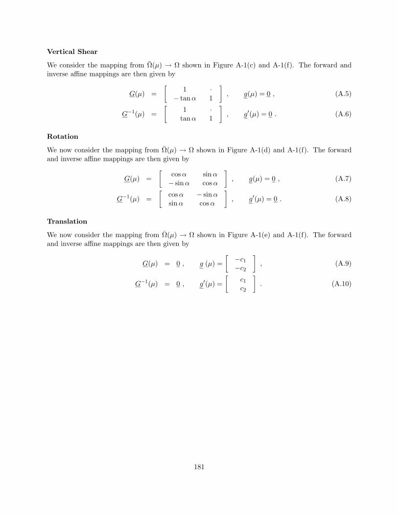
Vertical Shear

We consider the mapping from Ω(µ) → Ω shown in Figure A-1(c) and A-1(f). The forward andinverse affine mappings are then given by

G(µ) =[

1 ·− tanα 1

], g(µ) = 0 , (A.5)

G−1(µ) =[

1 ·tanα 1

], g′(µ) = 0 . (A.6)

Rotation

We now consider the mapping from Ω(µ) → Ω shown in Figure A-1(d) and A-1(f). The forwardand inverse affine mappings are then given by

G(µ) =[

cosα sinα− sinα cosα

], g(µ) = 0 , (A.7)

G−1(µ) =[

cosα − sinαsinα cosα

], g′(µ) = 0 . (A.8)

Translation

We now consider the mapping from Ω(µ) → Ω shown in Figure A-1(e) and A-1(f). The forwardand inverse affine mappings are then given by

G(µ) = 0 , g (µ) =[

−c1−c2

], (A.9)

G−1(µ) = 0 , g′(µ) =[

c1c2

]. (A.10)

181

182

Bibliography

[1] M. A. Akgun, J. H. Garcelon, and R. T. Haftka. Fast exact linear and non-linear structural re-analysis and the Sherman-Morrison-Woodbury formulas. International Journal for NumericalMethods in Engineering, 50(7):1587–1606, March 2001.

[2] S. Ali. TITLE. PhD thesis, SMA, 2003. In progress.

[3] E. Allgower and K. Georg. Simplicial and continuation methods for approximating fixed-pointsand solutions to systems of equations. SIAM Review, 22(1):28–85, 1980.

[4] B. O. Almroth, P. Stern, and F. A. Brogan. Automatic choice of global shape functions instructural analysis. AIAA Journal, 16:525–528, May 1978.

[5] A.C Antoulas and D.C. Sorensen. Approximation of large-scale dynamical systems: Anoverview. Technical report, Rice University, 2001.

[6] M. Avriel. Nonlinear Programming: Analysis and Methods. Prentice-Hall, Inc., EnglewoodCliffs, NJ, 1976.

[7] E. Balmes. Parametric families of reduced finite element models: Theory and applications.Mechanical Systems and Signal Processing, 10(4):381–394, 1996.

[8] A. Barrett and G. Reddien. On the reduced basis method. Z. Angew. Math. Mech., 75(7):543–549, 1995.

[9] D. Bertsekas. Nonlinear Programming. Athena Scientific, Belmont, MA, 2nd edition, 1999.

[10] T. F. Chan and W. L. Wan. Analysis of projection methods for solving linear systems withmultiple right-hand sides. SIAM Journal on Scientific Computing, 18(6):1698, 1721 1997.

[11] A. G. Evans, J. W. Hutchinson, N.A. Fleck, M. F. Ashby, and H. N. G. Wadley. The topologicaldesign of multifunctional cellular metals. Progress in Materials Science, 46(3-4):309–327, 2001.

[12] A.G. Evans. Private communication, 2001-2002.

[13] C. Farhat and F. X. Roux. Implicit parallel processing in structural mechanics. TechnicalReport CU-CSSC-93-26, Center for Aerospace Structures, University of Colorado, Boulder,CO, 1993.

[14] J. P. Fink and W. C. Rheinboldt. On the error behavior of the reduced basis technique fornonlinear finite element approximations. Z. Angew. Math. Mech., 63:21–28, 1983.

183

[15] A. Forsgren, P.E. Gill, and M.H. Wright. Interior methods for nonlinear optimization. SIAMReview, 44(4):535–597, 2002.

[16] L. J. Gibson and M. F. Ashby. Cellular Solids: Structure and Properties. Cambridge UniversityPress, 2nd edition, 1997.

[17] M. Grepl. PhD thesis, Massachusetts Institute of Technology, 2005. In progress.

[18] J. W. Hutchinson. Plastic buckling. In C.-S. Yih, editor, Advances in Applied Mechanics,volume 14, pages 67–144. Academic Press, Inc., 1974.

[19] J.W. Hutchinson. Private communication, 2001-2002.

[20] T. Leurent. Reduced basis output bounds for linear elasticity: Application to microtrussstructures. Master’s thesis, Massachusetts Institute of Technology, 2001.

[21] L. Machiels, Y. Maday, I. B. Oliveira, A.T. Patera, and D.V. Rovas. Output bounds forreduced-basis approximations of symmetric positive definite eigenvalue problems. C. R. Acad.Sci. Paris, Serie I, 331(2):153–158, July 2000.

[22] L. Machiels, Y. Maday, and A. T. Patera. A “flux-free” nodal Neumann subproblem approachto output bounds for partial differential equations. C. R. Acad. Sci. Paris, Serie I, 330(3):249–254, February 2000.

[23] L. Machiels, A.T. Patera, and D.V. Rovas. Reduced basis output bound methods for parabolicproblems. Computer Methods in Applied Mechanics and Engineering, 2001. Submitted.

[24] L. Machiels, J. Peraire, and A. T. Patera. A posteriori finite element output bounds for theincompressible Navier-Stokes equations; Application to a natural convection problem. Journalof Computational Physics, 172:401–425, 2001.

[25] Y. Maday, A. T. Patera, and J. Peraire. A general formulation for a posteriori bounds foroutput functionals of partial differential equations; Application to the eigenvalue problem. C.R. Acad. Sci. Paris, Serie I, 328:823–828, 1999.

[26] Y. Maday, A.T. Patera, and D.V. Rovas. A blackbox reduced-basis output bound method fornoncoercive linear problems. Nonlinear Partial Differential Equations and Their Applications,2001. Proceedings of the College De France Seminars.

[27] Y. Maday, A.T. Patera, and G. Turinici. A priori convergence theory for approximation ofsingle–parameter elliptic partial differential equations. C.R. Acad. Sci. Paris Serie I. Submit-ted.

[28] Y. Maday, A.T. Patera, and G. Turinici. A priori convergence theory for reduced–basis ap-proximations of single-parameter elliptic partial differential equations. Journal of ScientificComputing, 17(1–4):437–446, December 2002.

[29] L.E. Malvern. Introduction to the Mechanics of a Continuous Medium. Prentice-Hall, Inc.,1969.

184

[30] M.U. Nabi, V.R. Sule, and S.V. Kulkarni. An efficient computational modeling and solu-tion scheme for repeated finite element analysis of composite domains with varying materialproperty. International Journal of Computational Engineering Science, 3(3):257–275, 2002.

[31] A.W. Naylor and G.R. Sell. Linear Operator Theory in Engineering and Science, volume 40of Applied Mathematical Sciences. Springer-Verlag, New York, 1982.

[32] A. K. Noor and J. M. Peters. Reduced basis technique for nonlinear analysis of structures.AIAA Journal, 18(4):455–462, April 1980.

[33] I. Oliveira, C. Prud’homme, K. Veroy, and A.T. Patera. Thermo-structural anal-ysis of multifunctinoal prismatic cellular (triangular) metals. Web Publication,http://augustine.mit.edu, 2002.

[34] I. B. Oliveira and A. T. Patera. Reliable real-time optimization of nonconvex systems de-scribed by parametrized partial differential equations. In Proceedings Singapore-MIT AllianceSymposium, January 2003.

[35] A. T. Patera and E. M. Rønquist. A general output bound result: Application to discretizationand iteration error estimation and control. Math. Models Methods Appl. Sci., 11(4):685–712,2001.

[36] J. S. Peterson. The reduced basis method for incompressible viscous flow calculations. SIAMJ. Sci. Stat. Comput., 10(4):777–786, July 1989.

[37] T. A. Porsching. Estimation of the error in the reduced basis method solution of nonlinearequations. Mathematics of Computation, 45(172):487–496, October 1985.

[38] C. Prud’homme and A.T. Patera. Reduced-basis output bounds for approximatelyparametrized elliptic coercive partial differential equations. Computing and Visualization inScience, 2003. Accepted.

[39] C. Prud’homme, D. Rovas, K. Veroy, Y. Maday, A.T. Patera, and G. Turinici. Reliablereal-time solution of parametrized partial differential equations: Reduced-basis output boundsmethods. Journal of Fluids Engineering, 124(1):70–80, Mar 2002.

[40] C. Prud’homme, D. Rovas, K. Veroy, and A.T. Patera. Mathematical and computationalframework for reliable real–time solution of parametrized partial differential equations. M2AN,2002. Submitted.

[41] W.C. Rheinboldt. Numerical analysis of continuation methods for nonlinear structural prob-lems. Computers and Structures, 13(1-3):103–113, 1981.

[42] W.C. Rheinboldt. On the theory and error estimation of the reduced basis method for multi-parameter problems. Nonlinear Analysis, Theory, Methods and Applications, 21(11):849–858,1993.

[43] D. Rovas. Reduced-Basis Output Bound Methods for Partial Differential Equations. PhDthesis, Massachusetts Institute of Technology, 2002. In progress.

[44] I.H. Shames. Introduction to Solid Mechanics. Prentice Hall, New Jersey, 2nd edition, 1989.

185

[45] L. Sirovich and M. Kirby. Low-dimensional procedure for the characterization of human faces.Journal of the Optical Society of America A, 4(3):519–524, March 1987.

[46] Y. Solodukhov. (In progress). PhD thesis, Massachusetts Institute of Technology, 2004.

[47] K. Veroy, D. Rovas, and A.T. Patera. A posteriori error estimation for reduced-basis ap-proximation of parametrized elliptic coercive partial differential equations: “convex inverse”bound conditioners. Control, Optimisation and Calculus of Variations, 8:1007–1028, June2002. Special Volume: A tribute to J.-L. Lions.

[48] E. L. Yip. A note on the stability of solving a rank-p modification of a linear system by theSherman-Morrison-Woodbury formula. SIAM Journal on Scientific and Statistical Computat-ing, 7(2):507–513, April 1986.

186