Embed Size (px)
Citation preview
REDUCED KEPLER PROBLEM
IN ELLIPTIC COORDINATES
Nicholas Wheeler, Reed College Physics Department
March 1999
Introduction. The “2-body problem with central interaction” can be described
L = 12m1xxx1···xxx1 + 1
2m2xxx2···xxx2 − U(r)r ≡ length of rrr ≡ xxx2 − xxx1
but by familiar reduction—write
xxx1 = XXX + rrr1
xxx2 = XXX + rrr2
and require m1rrr1 + m2rrr2 = 000, giving
xxx1 = XXX − m2m1+m2
rrr
xxx2 = XXX + m1m1+m2
rrr
—assumes a form
L = 12MXXX···XXX +
12mrrr··· rrr − U(r)
with
M ≡ m1 + m2 : total massm ≡ m1m2
m1+m2: reduced mass
which can be considered to describe• motion rrr(t) of a fictitious “reduced mass” m in a central force field pinned
at the center of mass, superimposed upon• unaccelerated drift XXX(t) of the center of mass.
One is led thus from a physical 2-body problem to an abstractly equivalentone-body problem—the “reduced central force problem”
L = 12mrrr··· rrr − U(r) (1)
which in the case U(r) = −kr−1 becomes the “reduced Kepler problem.”Further reduction is made possible by the observation that, because the force iscentral, the orbit rrr(t) is confined necessarily to a central plane (i.e., to a planethat intersects the origin). That fact can be obtained as a corollary of a morerestrictive condition; namely, that (whether one argues by Noether’s theorem
2 Kepler problem in elliptic coordinates
from the rotational symmetry of (1), or from evaluation of the relevant Poissonbrackets) angular momentum is conserved :
LLL = 000 with LLL ≡ rrr×pppppp ≡ ∂L/∂rrr = mrrr
Evidently LLL stands normal to the orbital plane.
The 3-body problem (with gravitational interaction) is well-known to beanalytically intractable except in several classes of special cases, among whichis the “problem of two centers,” first studied by Leonard Euler. Euler imaginedtwo of the masses (M1 and M2) to be pinned (and their coordinates thereforeto be removed from the list of dynamical variables; the 3-body problem hasbecome at this point a one-body problem). The orbit of the third mass m isthen generally not confined to a plane, but—since m never experiences forcecomponents normal to the (M1,M2,m)-plane—will be so confined in pppinitial liesin that plane. It is to this case that Euler restricted his attention.
In a recent essay1 I had occasion to review, and in some respects to extend,Euler’s solution of the problem just described. Results appropriate to the Keplerproblem were obtained there by a several distinct limiting procedures. But thedensity of the argument was so great as frequently to obscure the significance ofthe results obtained. Here I will attempt to achieve a more focused account ofthe Keplerean significance of Euler’s method by eliminating all explicit referenceto Euler’s “second force center.” I will, of course, have things to say about thefamiliar “orbital” aspects of the Kepler problem, but will have special interest inthose aspects of its classical physics which relate more directly to the associatedquantum theory; orbital notions contributed centrally to Bohr’s account of thephysics of the hydrogen atom, but in the line of development which proceededhistorically from Bohr to Schrodinger such notions became progressively moresubordinate to ideas borrowed from Hamilton-Jacobi theory.
1. Reduced central force problem in polar coordinates. Erect—with origin atthe (inertial) force center—a Cartesian frame with (as a matter of convenience)z-axis aligned with LLL, and write
rrr =
x
y0
=
r cos θ
r sin θ0
Then
L = 12m(x2 + y2)− U
(√x2 + y2
)(2.1)
= 12m(r2 + r2θ2)− U(r) (2.2)
1 “Kepler problem by descent from the Euler problem” ().
Polar coordinates 3
givemx +
x√x2 + y2
· U ′(√x2 + y2)
= 0
my +y√
x2 + y2· U ′(√x2 + y2
)= 0
(3.1)
andmr + U ′(r)−mrθ2 = 0
ddt
[mr2θ
]= 0
(3.2)
respectively. Equations (3.1) are coupled except in the case U(r) = kr2, whichis the case of a 2-dimensional harmonic oscillator; m is bound to the force centerby a “spring.” Equations (3.2) are coupled in every case, but in every case onehas
mr2θ = constant with dimension of angular momentum, call it (4)
givingmr + U ′(r)− 2/mr3 = 0 (5)
from which all reference to θ has disappeared. Notice that we have achieved (5)not as an artifact of decoupling (of the sort exhibited by (3.1) in the harmoniccase) but by appeal to a conservation law; this is a circumstance recalled bythe 2 in (5). The conservation law in question can be expressed
pθ = 0 with pθ ≡ ∂∂θ
L = mr2θ : momentum conjugate to θ (6)= xpy− ypx
= (xxx× ppp)z
and arises because θ does not appear among the arguments of the Lagrangian;the polar coordinate system acquires its “universal pertinence” from the factthat it is adapted to the rotational symmetry of the central force problem(promotes the argument of U(•) to the status of a coordinate).
Further progress is made by appeal to energy conservation—as yetunexploited. From
E = 12m(r2 + r2θ2) + U(r)
= 12mr2 + U(r) + 1
22/mr2 (7)
we obtaindrdt =
√2m
[E − U(r)− 2
2mr2
](8)
at which point the dynamical problem has been “reduced to quadrature.”Further progress hinges upon one’s ability to• evaluate an integral;• execute a functional inversion;• evaluate another integral.
4 Kepler problem in elliptic coordinates
It would be pointless for me to pursue the details; they have been burnishedover the ages, and are well-described in (for example) Chapter 3 of Goldstein.2
I will confine my remarks to a few relatively non-standard points.
In dynamics generally—not just in connection with the 2-body problem—it is possible (and sometimes useful) to partition the “dynamical problem”(describe xxx(t)) into two parts:• construct a parameterized description xxx(λ) of the trajectory;• describe temporal progress λ(t) along that trajectory.
The former problem is, within the present context, usually interpreted as anassignment to construct r(θ), and is approached as follows:3 divide this variantof (4)
dθdt = /mr2
into (8) and obtain
drdθ = mr2
√2m
[E − U(r)− 2
2mr2
](9)
No θ appears on the right, so the problem has again been reduced to quadratureand a functional inversion—which, when they can be performed, yield r(θ;E, ).I digress now to describe an alternative derivation of (9).
Write r(θ) to describe a plane curve linking pointr1, θ1
to point
r2, θ2
.
The Euclidean length of such a curve C can be described∫ θ2
θ1
√r 2 + r2 dθ
where r ≡ dr/dθ. The mechanical analog of the “optical path length” of C isan attribute of C that becomes meaningful when we imagine the curve to havebeen traced with conserved energy E by a particle of mass m, and is given by4
A[r(t)] ≡∫ θ2
θ1
1n(r;E)
√r 2 + r2 dθ
1n(r;E)
≡√
2m
[E − U(r)
] (10)
Jacobi’s principle (the mechanical analog of Fermat’s principle of least time,sometimes known as the “principle of least action”) asserts that the physicaltrajectory
r1, θ1
−−−−−−−−−−−−−−−−−−−−−−−−−−−−−−−→
isoenergetic trajectory of particle with mass m
r2, θ2
2 H. Goldstein, Classical Mechanics (2nd edition, ). All future references
to “Goldstein” will be to this classic text.3 See §3–5 in Goldstein.4 See §5 in “Geometrical mechanics: Remarks commemorative of Heinrich
Hertz” ().
Polar coordinates 5
is the trajectory which extremizes A[r(θ)]:
δA[r(θ)] = 0 =⇒
ddθ
∂∂ r− ∂
∂ r
AE(r, r ) = 0 (11)
AE(r, r ) ≡√
2m
[E − U(r)
][r 2 + r2
]One could—with patience, on a large sheet of paper—actually write out thesecond order differential equation
G(r, r,˚r ) = 0 : mechanical analog of the optical “ray equation”
of which (11) speaks, but the result (I am informed by Mathematica) is a mess:that, evidently, is not the way to go; some circumspection is called for. Iproceed in geometrical/non-temporal mimicry of a line of argument standardto temporal mechanics.
Lagrangian dynamics supplies the general proposition that if L(q, q) doesnot depend explicitly on t then J(q, q) ≡ L− q ·(∂L/∂q) is a constant of motion:
∂∂tL = 0 =⇒ J(q, q) = constant
J(q, q) is “Jacobi’s integral”—interpretable as “total energy” T +U in its mostcommonly-encountered manifestations, and recommended to our attention byNoether’s theorem as the object of interest whenever time-translation is amap of interest. All of which has much to do with the abstract calculus ofvariations, and only incidentally to do—by way of “illustrative application”—with dynamics. Looking in this light back now to (11), we observe that AE(r, r )displays no explicit dependence upon the independent variable θ: ∂
∂θAE = 0.The implication is that
J(r, r ) ≡ AE − r · (∂AE/∂ r ) (12.1)
has the property that ∂∂θJ(r, r ) vanishes on every solution r(θ) of (11):
J(r, r ) is constant on every trajectory (12.2)
The argument culminating in (12) is of some general interest: it alerts us to thefact that Noether’s theorem possesses a domain of applicability which extendsfar beyond the dynamical domain with which we physicists are most familiar.5
But concentrating now on the particulars of the situation, we have
J =√
2m
[E − U
][r 2 + r2
]− r ·
2m
[E − U
]r√
2m
[E − U
][r 2 + r2
]=
2m
[E − U
][r 2 + r2 − r 2
]√2m
[E − U
][r 2 + r2
]5 I suspect that the non-dynamical (geometrical) manifestations of her train
of thought were known long before Noether herself entered the picture, andthat she was familiar with them, but I have not had opportunity to discoverwhether the historical literature supports my suspicion.
6 Kepler problem in elliptic coordinates
giving
J(r, r ) = r2
√E − U(r)r 2 + r2
= constant, call it√
2/2m (13)
This is precisely equivalent to (9). Recent discussion has taught us nothing wedid not already know about orbital geometry in central force problems, but it isinteresting to see that (and how) the variational principle (11)—which pertainsin principle to a much broader class of problems—can be made to do usefulwork. And the discussion has served to alert us to the geometrical potentialitiesof Noether’s theorem.
The orbital equation (13) can be written
r 2 = r2
E − U(r)2/2mr2
− 1
= (2mr4/2)E − U(r)− 2/2mr2
(14.1)
= (2mr4/2)E − Ueff(r; 2)
(14.2)
Ueff(r; 2) ≡ 2
2mr2 + U(r) (15)
A change of variable r → z ≡ 1/r (which entails r → z = − r /r2) permits thisresult to be cast into a form
12mz 2 = E− V (z) with
E ≡ (m/)2EV (z) ≡ (m/)2Ueff(z−1; 2)
which makes even more obvious the fact that (14) presents a problem which isabstractly equivalent to the problem of a particle moving one-dimensionally ina potential well; the role of time t has been taken over now by a geometricalvariable θ, and z has the dimension of reciprocal length, but—those distinctionsnotwithstanding—the imagery of the latter problem can be borrowed intact:orbits are excluded from regions where E − V (z) < 0, are confined to theinterior of annular regions bounded by the analog of “turning points,” becomecircular at the analog of stable/unstable “equilibrium points.” Orbits passingthrough a point r(θ) are• destined to collapse (r → 0)• bounded (r is oscillatory, a periodic function of θ)• destined to evaporate (r →∞)
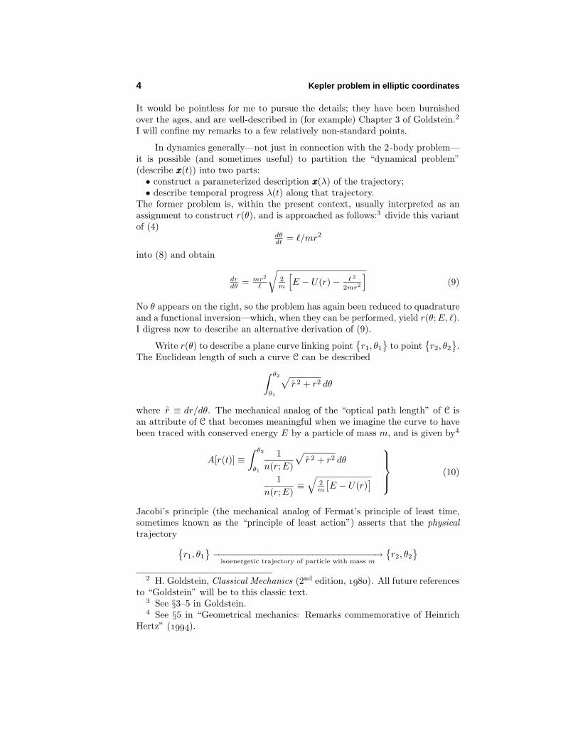
according to the placement of the nearest turning points, and that placementdepends upon the values which have been assigned to the physical parametersE and 2 (which can usefully be considered to mark a point on a semi-infinite“control plane”). Typical aspects of the situation are illustrated in Figure 1.
In view of my destination, and to eliminate distracting complications inthe shorter term, I restrict my attention now and henceforth to the power-lawpotentials
U(r) = krn (16)
Polar coordinates 7
1 2 3 4 5
-2
2
4
6
8
10
Figure 1: I have, for illustrative purposes, assigned the potentialenergy function the physically artificial structure
U(r) = ae−br sin cr
and plotted Ueff(r, 2). From such figures one can, for each assignedvalue of E, read off orbital turning point data. Here identical valuesof E and 2 support both
a bound orbit with 0.9 r 2.3, andan unbound orbit with 2.8 r
Analogous figures arise from each assigned value of 2. For the2-value shown, no orbit is possible if E < 2.2. The spike on theleft arises from the 2/2mr2-term which enters additively into thedefinition of Ueff(r, 2).
and will give special attention to the
harmonic potential: U(r) = +kr2
attractive coulomb potential (kepler problem): U(r) = −kr−1
where the “strength parameter” k is taken in both cases to be positive. Graphstypical of Ueff(r, 2) in those two cases are shown in Figure 2. Also worthy ofspecial mention is the “super-Coulombic case” U(r) = −kr−2 which, thoughphysically unimportant, acquires theoretical interest from several interrelatedcircumstances: the associated effective potential can be written
Ueff(r, 2) =
2
2m − kr−2
which presents only a single power or r; bound orbits are possible only if2 < 2mk, and such orbits are unstable against collapse. Of deeper interest
8 Kepler problem in elliptic coordinates
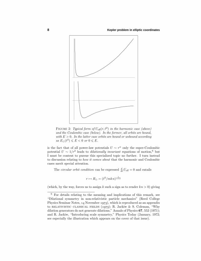
Figure 2: Typical form of Ueff(r, 2) in the harmonic case (above)and the Coulombic case (below). In the former, all orbits are bound,with E > 0. In the latter case orbits are bound or unbound accordingas E(2) E < 0 or 0 E.
is the fact that of all power-law potentials U ∼ rn only the super-Coulombicpotential U ∼ 1/r2 leads to dilationally invariant equations of motion,6 butI must be content to pursue this specialized topic no further. I turn insteadto discussion relating to how it comes about that the harmonic and Coulombiccases merit special attention.
The circular orbit condition can be expressed ddrUeff = 0 and entails
r → R = (2/mkn)1
n+2
(which, by the way, forces us to assign k such a sign as to render kn > 0) giving
6 For details relating to the meaning and implications of this remark, see“Dilational symmetry in non-relativistic particle mechanics” (Reed CollegePhysics Seminar Notes, November ), which is reproduced as an appendixto relativistic classical fields (); R. Jackiw & S. Coleman, “Whydilation generators do not generate dilations,” Annals of Physics 67, 552 (1971);and R. Jackiw, “Introducing scale symmetry,” Physics Today (January, 1972;see especially the illustration which appears on the cover of that issue).
Polar coordinates 9
2-dependent radius of circular orbit R =
(2/2mk)1/4 : case n = +2(2/mk) : case n = −1
Such orbits are pursued with energy
E(2) = √
2k2/m = 2U(R) : case n = +2− 1
2mk2/2 = 12U(R) : case n = −1
and these results—written
E(2) = T + U(R) with
T = +1U(R) : case n = +2T = − 1
2U(R) : case n = −1
—are found to be consistent with assertions of the virial theorem.7 Location ofthe turning points requires that we discover real solutions (when they exist) of
krn+2 − Er2 + 2/2m = 0
which generally cannot be accomplished in closed form. But in the harmoniccase we have
kr4 − Er2 + 2/2m = 0
giving
r2 =E ±
√E2 − 2k2/m
2k: necessarily E2 2k2/m = E2
whence
rmin (E, 2) =[E −
√E2 − 2k2/m
2k
] 12
R(2)
rmax(E, 2) =[E +
√E2 − 2k2/m
2k
] 12
R(2)
which coalesce as E ↓ E and become imaginary (unphysical) if E < E. Inthe Coulombic (Keplerean) case we have
Er2 + kr − 2/2m = 0
and find that we must distinguish• elliptic cases E E < 0 from• parabolic cases E = 0 from• hyperbolic cases E > 0.
The relatively fussy details are developed in §6. Such details are of interest ina variety of connections, and serve indispensably as aids to setting parametersand initial conditions in numerical work such as that to which I now turn.
7 Goldstein, §3–4. In the general case we expect, on this elegant basis, tohave T = n
2U(R).

10 Kepler problem in elliptic coordinates
One might naively suppose that, having selected a potential U(r) andassigned values to E, 2 and r (0), one has only to integrate (9)—numericallyif not analytically—to obtain a description of the implied orbit r(θ). But acomputational problem (whichMathematica was quick to bring to my attention)arises from the circumstance that (9) should properly be written
r = ±mr2
√2m
[E − U(r)− 2
2mr2
](17)
where the sign is ± on ascending/descending sectors of an orbit; it flips +→ −as r(θ) passes through rmax, and flips again − → + as r(θ) passes throughrmin. Any successful orbit-generating algorithm based upon (17) will containnecessarily some sign-selection sub-routine, and this my rudimentary numericalskills have not permitted me to accomplish. I need graphical representations oforbits to make my expository point, so I temporarily retreat to the elementaryCartesian t -parameterized dynamics of the problem, working from
mx = −kn(x2 + y2)n−2
2 x
my = −kn(x2 + y2)n−2
2 y
(18)
though it hurts to do so: (17) is a single first-order equation, phrased in termsthat relate directly to the geometrical problem of interest, while (18) is a pairof second-order equations which relate only incidentally orbital geometry.
To study the qualitative implications of (18) we write those equations insimplified canonical form
x = uu = −(x2 + y2)
n−22 x
y = vv = −(x2 + y2)
n−22 y
and set x0 = 1, u0 = y0 = 0. If, additionally, we set v0 = 1 then the resultingorbit is found in all cases—irrespective of the value assigned to n—to be a unitcircle, centered at the origin. Thus nicely positioned in parameter space, we(to obtain orbits with informative shape) tweek the launch speed (set v0 = 0.5)and draw the orbits which result when• n lies in the neighborhood of its harmonic value n = +2;• n lies in the neighborhood of its Coulombic value n = −1. The results are
displayed in Figures 3 & 4, which are intended to lend experimental weight tothe following claim:
Precession is the rule, orbital closure the exception. For any given powerlaw U ∼ rn the bound-orbital sector of the parameter space
E, 2
is peppered
with points that give rise to closed/periodic orbits, but only in the harmonicand Coulombic cases is every bound orbit closed (and, as it happens, elliptical,with center at the force center in the former case, focus at the force center in

Polar coordinates 11
the latter case). This is the upshot of “Bertrand’s theorem,”8 which did notattract general interest until soon after the invention of quantum mechanics,when it was noticed—first by Pauli ()—that there appears to be a deepand significant connection between• orbital closure,• multiple separability of the Schrodinger equation,• “accidental degeneracy” of the quantum mechanical energy spectrum.9
This circumstance accounts for the fact that it is to be best modern texts thatone must look to find discussion of the proof of Bertrand’s theorem.10 Herewe will be concerned mainly with aspects of the multi-separability issue.
8 Joseph L. P. Bertrand (–), who received his doctorate at seventeen,made important contributions to pure mathematics, theoretical mechanics,thermodynamics and several other fields (he wrote on the flight of birds), wasthe author of several influential texts, and ultimately acquired virtually everyscholarly distinction his native France had to bestow. “Bertrand’s theorem”was published in Comptes Rendus 77, 849 (1873). It was ignored by authors ofmost of the older monographs, but is discussed in §428 of E. J. Routh’s Treatiseon the Dynamics of a Particle ().
9 For an accessible account of this pretty subject—which appears to retainmuch mystery—see H. V. McIntosh, “On accidental degeneracy in classical andquantum mechanics,” AJP 27, 620 (1959) and classic papers cited there; also“Symmetry and degeneracy” in Group Theory and its Applications II , edited byE. M. Loebl (). Relevant material can be found in classical dynamics,Chapter 9, pp. 61–74 ().
10 Goldstein devotes his §3–6 to discussion of some implications of Bertrand’stheorem, and in his Appendix A presents a detailed proof. Valuable discussioncan be found also in §2.3.3 of J. V. Jose & E. J. Saletan, Classical Dynamics:A Contemporary Approach () and—which I especially recommend—§§4.4/5of J. L. McCauley, Classical Mechanics: Transformations, Flows, Integrable& Chaotic Dynamics (). It is my impression, however, that the worldstill awaits the development of a truly illuminating account of the origin andramifications of Bertrand’s theorem.
12 Kepler problem in elliptic coordinates
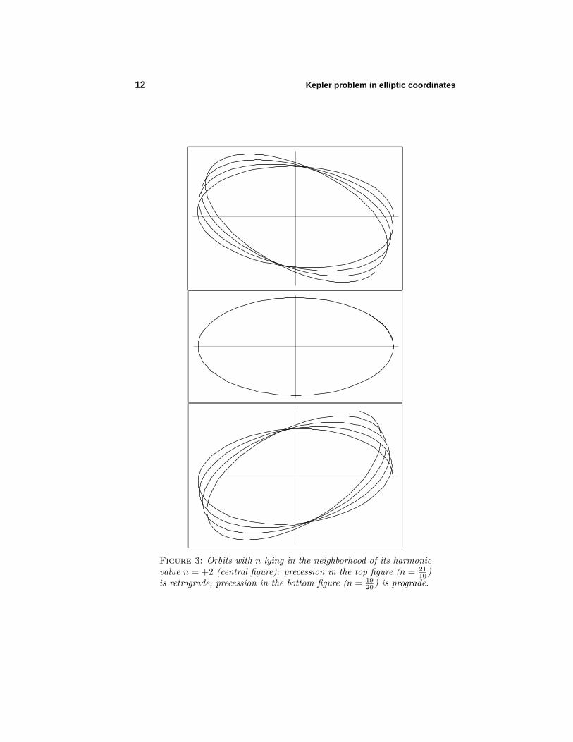
Figure 3: Orbits with n lying in the neighborhood of its harmonicvalue n = +2 (central figure): precession in the top figure (n = 21
10)is retrograde, precession in the bottom figure (n = 19
20) is prograde.

Polar coordinates 13
14 Kepler problem in elliptic coordinates
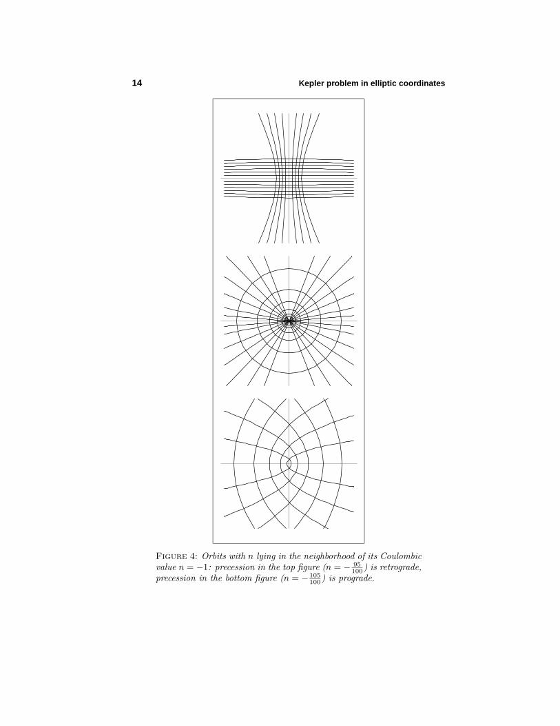
Figure 4: Orbits with n lying in the neighborhood of its Coulombicvalue n = −1: precession in the top figure (n = − 95
100) is retrograde,precession in the bottom figure (n = − 105
100) is prograde.
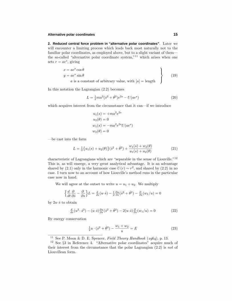
Alternative polar coordinates 15
2. Reduced central force problem in “alternative polar coordinates”. Later wewill encounter a limiting process which leads back most naturally not to thefamiliar polar coordinates, as employed above, but to a slight variant of them—the so-called “alternative polar coordinate system,”11 which arises when onesets r = aes, giving
x = aes cos θy = aes sin θ
a is a constant of arbitrary value, with [a] = length
(19)
In this notation the Lagrangian (2.2) becomes
L = 12ma2(s2 + θ2)e2s − U(aes) (20)
which acquires interest from the circumstance that it can—if we introduce
u1(s) = +ma2e2s
u2(θ) = 0
w1(s) = −ma2e2sU(aes)w2(θ) = 0
—be cast into the form
L = 12
u1(s) + u2(θ)
(s2 + θ2) +
w1(s) + w2(θ)u1(s) + u2(θ)
(21)
characteristic of Lagrangians which are “separable in the sense of Liouville.”12
This is, as will emerge, a very great analytical advantage. It is an advantageshared by (2.1) only in the harmonic case U(r) ∼ r2, and shared by (2.2) in nocase. I turn now to an account of how Liouville’s method runs in the particularcase now in hand.
We will agree at the outset to write u = u1 + u2. We multiplyddt
∂∂s− ∂
∂s
L = d
ds (u·s)− 12∂u∂s (s2 + θ2)− ∂
∂s (w1/u) = 0
by 2u·s to obtain
dds (u
2 · s2)− (u·s)∂u∂s (s2 + θ2)− 2(u·s) ∂∂s (w1/u) = 0 (22)
By energy conservation
12u · (s2 + θ2)− w1 + w2
u= E (23)
11 See P. Moon & D. E. Spencer, Field Theory Handbook (), p. 13.12 See §3 in Reference 4. “Alternative polar coordinates” acquire much of
their interest from the circumstance that the polar Lagrangian (2.2) is not ofLiouvillean form.
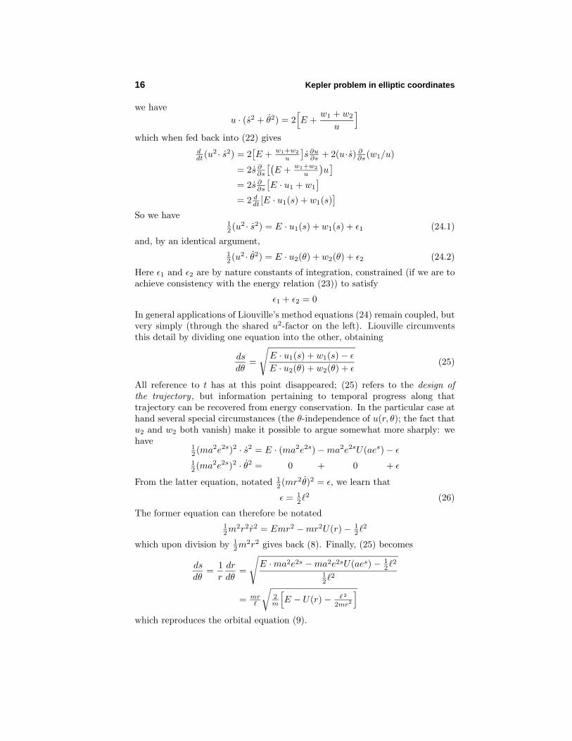
16 Kepler problem in elliptic coordinates
we haveu · (s2 + θ2) = 2
[E +
w1 + w2
u
]which when fed back into (22) gives
ddt (u
2 · s2) = 2[E + w1+w2
u
]s∂u∂s + 2(u·s) ∂
∂s (w1/u)
= 2s ∂∂s
[(E + w1+w2
u
)u
]= 2s ∂
∂s
[E · u1 + w1
]= 2 d
dt [E · u1(s) + w1(s)]
So we have12 (u2 · s2) = E · u1(s) + w1(s) + ε1 (24.1)
and, by an identical argument,12 (u2 · θ2) = E · u2(θ) + w2(θ) + ε2 (24.2)
Here ε1 and ε2 are by nature constants of integration, constrained (if we are toachieve consistency with the energy relation (23)) to satisfy
ε1 + ε2 = 0
In general applications of Liouville’s method equations (24) remain coupled, butvery simply (through the shared u2-factor on the left). Liouville circumventsthis detail by dividing one equation into the other, obtaining
ds
dθ=
√E · u1(s) + w1(s)− ε
E · u2(θ) + w2(θ) + ε(25)
All reference to t has at this point disappeared; (25) refers to the design ofthe trajectory , but information pertaining to temporal progress along thattrajectory can be recovered from energy conservation. In the particular case athand several special circumstances (the θ-independence of u(r, θ); the fact thatu2 and w2 both vanish) make it possible to argue somewhat more sharply: wehave
12 (ma2e2s)2 · s2 = E · (ma2e2s)−ma2e2sU(aes)− ε
12 (ma2e2s)2 · θ2 = 0 + 0 + ε
From the latter equation, notated 12 (mr2θ)2 = ε, we learn that
ε = 12
2 (26)
The former equation can therefore be notated12m
2r2r2 = Emr2 −mr2U(r)− 12
2
which upon division by 12m
2r2 gives back (8). Finally, (25) becomes
ds
dθ= 1
r
dr
dθ=
√E ·ma2e2s −ma2e2sU(aes)− 1
22
12
2
= mr
√2m
[E − U(r)− 2
2mr2
]which reproduces the orbital equation (9).
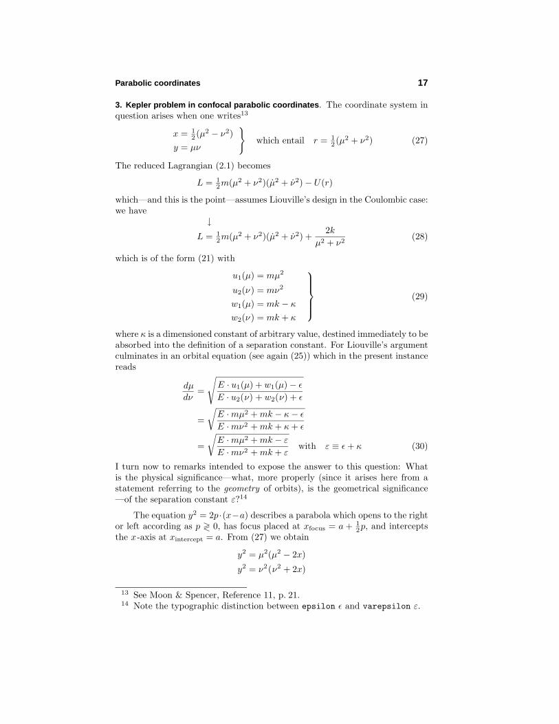
Parabolic coordinates 17
3. Kepler problem in confocal parabolic coordinates. The coordinate system inquestion arises when one writes13
x = 12 (µ2 − ν2)
y = µν
which entail r = 1
2 (µ2 + ν2) (27)
The reduced Lagrangian (2.1) becomes
L = 12m(µ2 + ν2)(µ2 + ν2)− U(r)
which—and this is the point—assumes Liouville’s design in the Coulombic case:we have
↓L = 1
2m(µ2 + ν2)(µ2 + ν2) +2k
µ2 + ν2(28)
which is of the form (21) with
u1(µ) = mµ2
u2(ν) = mν2
w1(µ) = mk − κ
w2(ν) = mk + κ
(29)
where κ is a dimensioned constant of arbitrary value, destined immediately to beabsorbed into the definition of a separation constant. For Liouville’s argumentculminates in an orbital equation (see again (25)) which in the present instancereads
dµ
dν=
√E · u1(µ) + w1(µ)− ε
E · u2(ν) + w2(ν) + ε
=
√E ·mµ2 + mk − κ− ε
E ·mν2 + mk + κ + ε
=
√E ·mµ2 + mk − ε
E ·mν2 + mk + εwith ε ≡ ε + κ (30)
I turn now to remarks intended to expose the answer to this question: Whatis the physical significance—what, more properly (since it arises here from astatement referring to the geometry of orbits), is the geometrical significance—of the separation constant ε?14
The equation y2 = 2p ·(x−a) describes a parabola which opens to the rightor left according as p ≷ 0, has focus placed at xfocus = a + 1
2p, and interceptsthe x-axis at xintercept = a. From (27) we obtain
y2 = µ2(µ2 − 2x)
y2 = ν2(ν2 + 2x)
13 See Moon & Spencer, Reference 11, p. 21.14 Note the typographic distinction between epsilon ε and varepsilon ε.
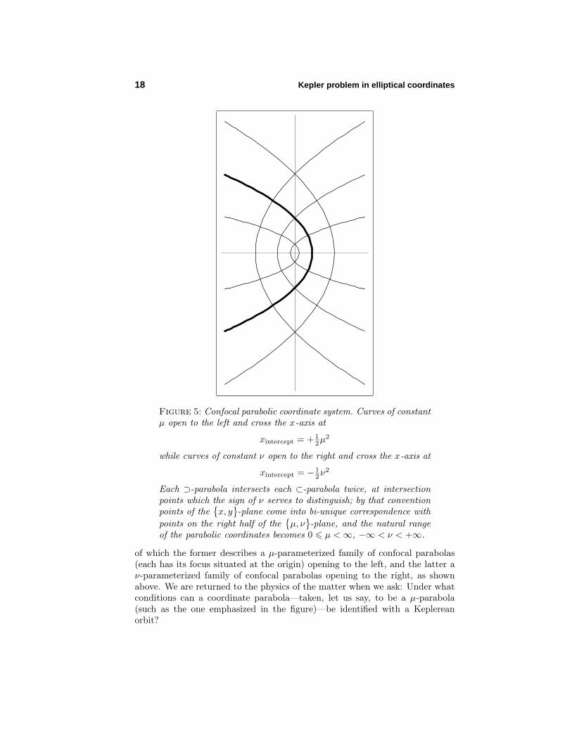
18 Kepler problem in elliptical coordinates
Figure 5: Confocal parabolic coordinate system. Curves of constantµ open to the left and cross the x-axis at
xintercept = + 12µ
2
while curves of constant ν open to the right and cross the x-axis at
xintercept = − 12ν
2
Each ⊃-parabola intersects each ⊂-parabola twice, at intersectionpoints which the sign of ν serves to distinguish; by that conventionpoints of the
x, y
-plane come into bi-unique correspondence with
points on the right half of theµ, ν
-plane, and the natural range
of the parabolic coordinates becomes 0 µ <∞, −∞ < ν < +∞.
of which the former describes a µ-parameterized family of confocal parabolas(each has its focus situated at the origin) opening to the left, and the latter aν-parameterized family of confocal parabolas opening to the right, as shownabove. We are returned to the physics of the matter when we ask: Under whatconditions can a coordinate parabola—taken, let us say, to be a µ-parabola(such as the one emphasized in the figure)—be identified with a Keplereanorbit?
Elliptic coordinates 19
4. The confocal elliptic coordinate system. The coordinate system now inquestion arises when one writes15
x = a cosh ξ cos ηy = a sinh ξ sin η
(31)
and assumesξ, η
to range on a semi-infinite strip: 0 ξ < ∞, 0 η < 2π.
Elimination first of η, then of ξ, gives( x
a cosh ξ
)2
+( y
a sinh ξ
)2
= 1( x
a cos η
)2
−( y
a sin η
)2
= 1
(32)
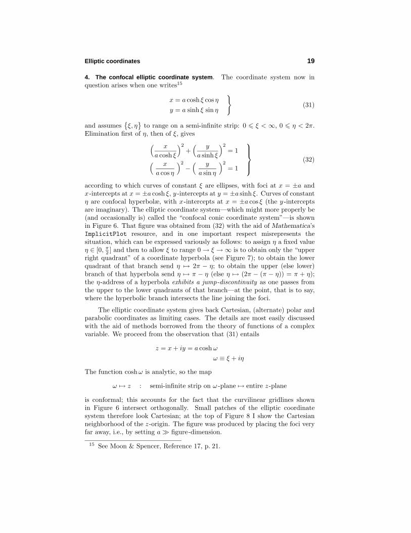
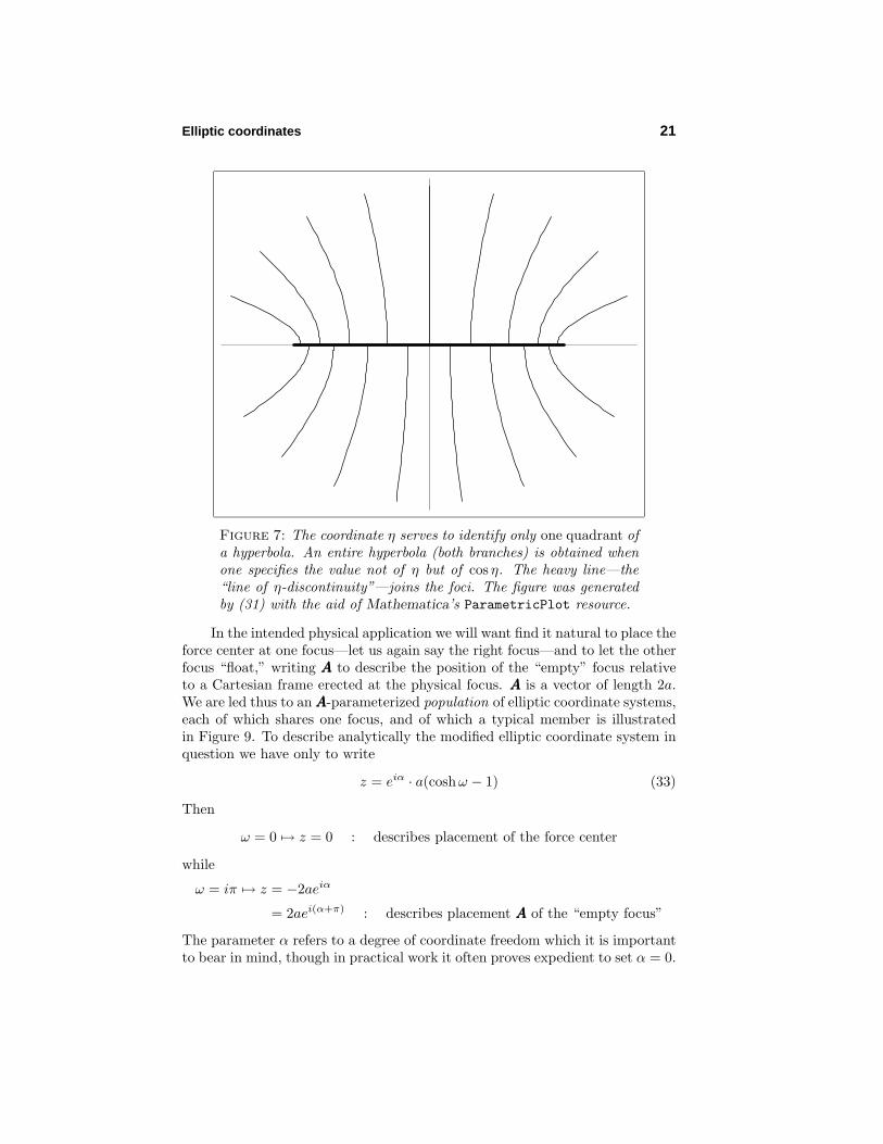
according to which curves of constant ξ are ellipses, with foci at x = ±a andx-intercepts at x = ±a cosh ξ, y -intercepts at y = ±a sinh ξ. Curves of constantη are confocal hyperbolæ, with x-intercepts at x = ±a cos ξ (the y -interceptsare imaginary). The elliptic coordinate system—which might more properly be(and occasionally is) called the “confocal conic coordinate system”—is shownin Figure 6. That figure was obtained from (32) with the aid of Mathematica’sImplicitPlot resource, and in one important respect misrepresents thesituation, which can be expressed variously as follows: to assign η a fixed valueη ∈ [0, π2 ] and then to allow ξ to range 0→ ξ →∞ is to obtain only the “upperright quadrant” of a coordinate hyperbola (see Figure 7); to obtain the lowerquadrant of that branch send η → 2π − η; to obtain the upper (else lower)branch of that hyperbola send η → π − η (else η → (2π − (π − η)) = π + η);the η-address of a hyperbola exhibits a jump-discontinuity as one passes fromthe upper to the lower quadrants of that branch—at the point, that is to say,where the hyperbolic branch intersects the line joining the foci.
The elliptic coordinate system gives back Cartesian, (alternate) polar andparabolic coordinates as limiting cases. The details are most easily discussedwith the aid of methods borrowed from the theory of functions of a complexvariable. We proceed from the observation that (31) entails
z = x + iy = a cosh ω
ω ≡ ξ + iη
The function coshω is analytic, so the map
ω → z : semi-infinite strip on ω -plane → entire z-plane
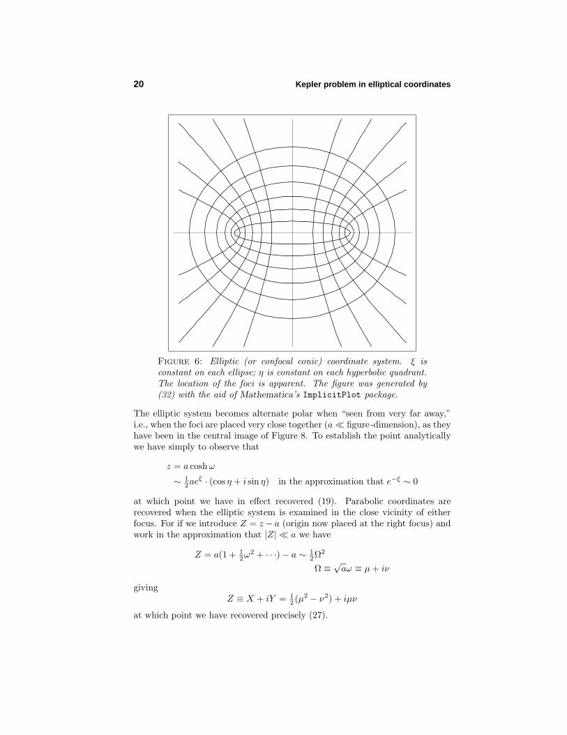
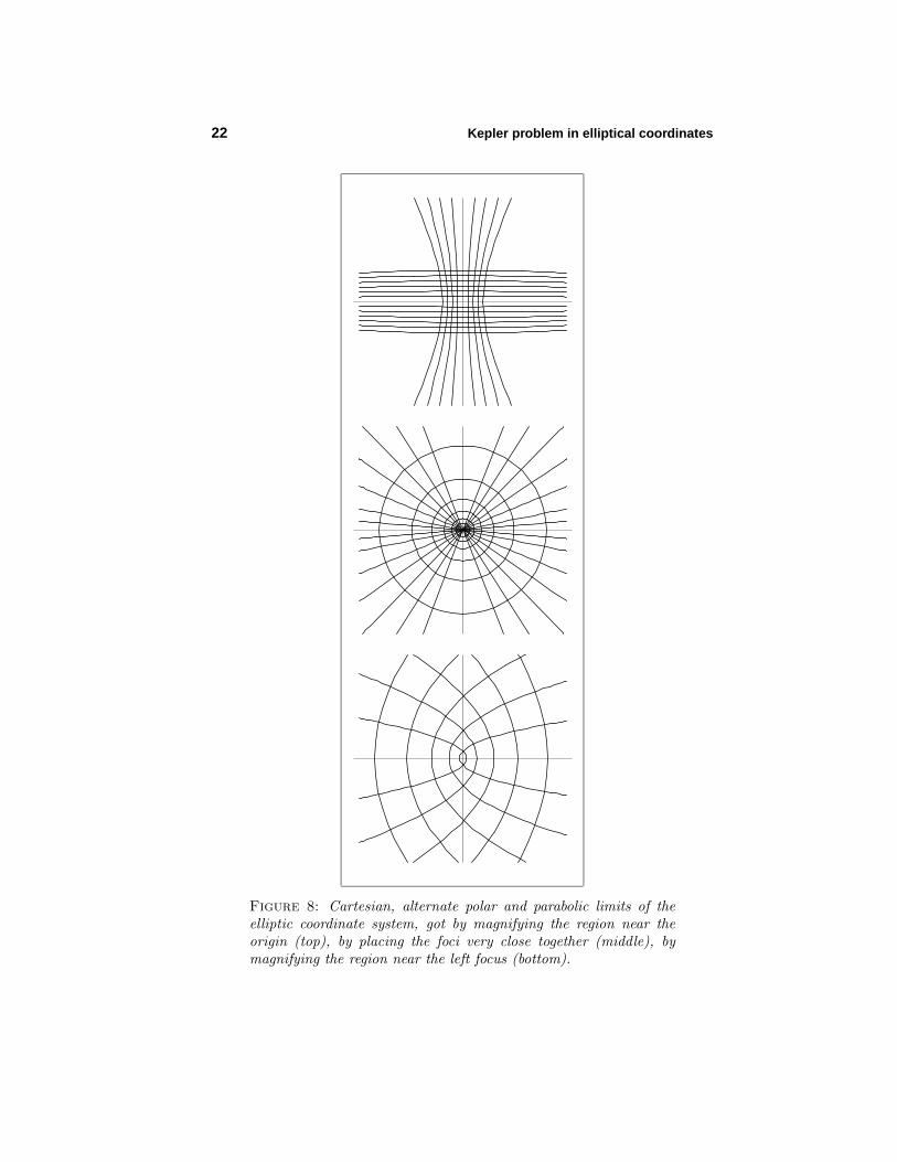
is conformal; this accounts for the fact that the curvilinear gridlines shownin Figure 6 intersect orthogonally. Small patches of the elliptic coordinatesystem therefore look Cartesian; at the top of Figure 8 I show the Cartesianneighborhood of the z-origin. The figure was produced by placing the foci veryfar away, i.e., by setting a figure-dimension.
15 See Moon & Spencer, Reference 17, p. 21.
20 Kepler problem in elliptical coordinates
Figure 6: Elliptic (or confocal conic) coordinate system. ξ isconstant on each ellipse; η is constant on each hyperbolic quadrant.The location of the foci is apparent. The figure was generated by(32) with the aid of Mathematica’s ImplicitPlot package.
The elliptic system becomes alternate polar when “seen from very far away,”i.e., when the foci are placed very close together (a figure-dimension), as theyhave been in the central image of Figure 8. To establish the point analyticallywe have simply to observe that
z = a coshω
∼ 12ae
ξ · (cos η + i sin η) in the approximation that e−ξ ∼ 0
at which point we have in effect recovered (19). Parabolic coordinates arerecovered when the elliptic system is examined in the close vicinity of eitherfocus. For if we introduce Z = z− a (origin now placed at the right focus) andwork in the approximation that |Z| a we have
Z = a(1 + 12ω
2 + · · ·)− a ∼ 12Ω2
Ω ≡√aω ≡ µ + iν
givingZ ≡ X + iY = 1
2 (µ2 − ν2) + iµν
at which point we have recovered precisely (27).
Elliptic coordinates 21
Figure 7: The coordinate η serves to identify only one quadrant ofa hyperbola. An entire hyperbola (both branches) is obtained whenone specifies the value not of η but of cos η. The heavy line—the“line of η-discontinuity”—joins the foci. The figure was generatedby (31) with the aid of Mathematica’s ParametricPlot resource.
In the intended physical application we will want find it natural to place theforce center at one focus—let us again say the right focus—and to let the otherfocus “float,” writing AAA to describe the position of the “empty” focus relativeto a Cartesian frame erected at the physical focus. AAA is a vector of length 2a.We are led thus to an AAA-parameterized population of elliptic coordinate systems,each of which shares one focus, and of which a typical member is illustratedin Figure 9. To describe analytically the modified elliptic coordinate system inquestion we have only to write
z = eiα · a(coshω − 1) (33)
Then
ω = 0 → z = 0 : describes placement of the force center
while
ω = iπ → z = −2aeiα
= 2aei(α+π) : describes placement AAA of the “empty focus”
The parameter α refers to a degree of coordinate freedom which it is importantto bear in mind, though in practical work it often proves expedient to set α = 0.
22 Kepler problem in elliptical coordinates
Figure 8: Cartesian, alternate polar and parabolic limits of theelliptic coordinate system, got by magnifying the region near theorigin (top), by placing the foci very close together (middle), bymagnifying the region near the left focus (bottom).

Elliptic coordinates 23
Figure 9: Keplerean modification of the elliptic coordinate system.The standard system has been first translated (top figure) so as toplace a focus at the origin (force center), and then rotated (bottomfigure). The heavy ellipse alludes to the possibility of identifyingcoordinate lines with Keplerean orbits.
The polar and parabolic coordinate systems give rise to populations ofcoordinate lines which can in both cases be associated with subsets of the setof all possible Keplerean orbits (i.e., with the set of all conic sections whichhave a focus at the origin). It is, in this respect, a striking—and potentiallyuseful—property of the elliptic system(s) that
every Keplerean orbit can be associated with one or anotherof the coordinate lines supplied by some elliptic system;
one has only to assign appropriate values to AAA and ξ (else η). Moreover, thevector AAA (which is to say: the location of the empty focus) acquires the statusof a constant of the motion. I return to this topic in §6.
With all preparations now behind us, we are in position at last to turn toreview of the formal mechanical essentials of the topic announced in the title:

24 Kepler problem in elliptical coordinates
5. Physical application: the Kepler problem. The reduced Lagrangian (1) can,in the Keplerean case,16 be notated
L = 12mz∗z + k 1√
z∗z
= 12ma2(sinhω)∗(sinhω) · ω∗ω + k 1
a√
(coshω − 1)∗(coshω − 1)
which with the aid of
sinhω = sinh ξ cos η + i cosh ξ sin η
coshω = cosh ξ cos η + i sinh ξ sin η
⇓(sinhω)∗(sinhω) = cosh2 ξ − cos2 η
(coshω − 1)∗(coshω − 1) = (cosh ξ − cos η)2
becomes
L = 12ma2(cosh2 ξ − cos2 η)(ξ2 + η2) + k
cosh ξ + cos ηa(cosh2 ξ − cos2 η)
(34)
But (34) is of the design (21) with
u1(ξ) = +ma2 cosh2 ξ
u2(η) = −ma2 cos2 η
w1(ξ) = kma cosh ξ
w2(ξ) = kma cos η
(35)
and is therefore “separable in the sense of Liouville.” The remarkableimplication is that the Kepler problem is separable not only in polar andparabolic coordinates (separability in those cases is well known) but in eachof the confocal elliptic systems (33), where “each” means “irrespective of thevalues ascribed to a and to α” (in short: for all AAA). Polar/parabolic separabilitycan be understood to arise as limiting consequences of this exceptional fact.
Working from (33) we find that the momenta conjugate to ξ and η can bedescribed
pξ = uξ
pη = uη
u ≡ u1(ξ) + u2(η) = ma2(cosh2 ξ − cos2 η)
16 Generally I reserve “Keplerean” for problems in which the interaction is(attractive) gravitational (k = GMm), and—as previously—use “Coulombic”when the sign and physical interpretation of k are non-specific. In the presentcontext I find it artificial to maintain that convention.

Mechanical essentials 25
and that the associated Hamiltonian H = pξ ξ + pη η − L can therefore berendered
H = 12u
(p2ξ + p2
η
)− 2(w1 + w2)
(36)
= 12ma2
1
cosh2 ξ − cos2 η(p2
ξ + p2η)− 2kma 1
cosh ξ − cos η
Eliminating E between Liouville’s equations (24)—which in the present instanceread
12 (u2 · ξ2) = E · u1(ξ) + w1(ξ)− ε12 (u2 · η2) = E · u2(η) + w2(η) + ε
—we obtain
ε = − 12u · (u2 ξ
2 − u1η2) + u2w1 − u1w2
u
↓G = − 1
2u
(u2p
2ξ − u1p
2η
)− 2
(u2w1 − u1w2
)(37)
= 12
1
cosh2 ξ − cos2 η
(p2ξ cos2 η + p2
η cosh2 ξ)− 2kma
cosh ξ cos ηcosh ξ − cos η
Here ε, which came to us as a “separation constant in the sense of Liouville,”has been promoted to the status of an observable, which I will call “Liouville’sobservable.” With the indispensable assistance of Mathmatica we confirm—whether we work from the generic or the elliptic-specific versions of (36) and(37)—that the Poisson bracket
[H,G ] = 0
according to which ε acquires this interpretation:
ε = dynamically conserved value of G(pξ, pη, ξ, η)
But that observation, while it shifts the locus, leaves unanswered the question:What is the “meaning” of ε? I approach the question by specialization of themethods and results developed in §§4–6 of an essay previously cited.1
Keplerean orbits are standardly classified by specification of the conservedvalues of H, LLL and KKK, where
H ≡ 12m ppp···ppp− k
r : HamiltonianLLL ≡ rrr × ppp : angular momentum vectorKKK ≡ 1
m (ppp×LLL)− kr rrr (38)
= 1m
[(ppp···ppp)rrr − (rrr···ppp)ppp
]− k
r rrr : Lenz vector
26 Kepler problem in elliptical coordinates
and only the last of those is at all unfamiliar.17 Clearly KKK ⊥ LLL, and sinceLLL stands normal to the orbital plane, KKK lies in the orbital plane. We have,by convention, identified the orbital plane with the
x, y
-plane, and therefore
have
LLL =
0
0Lz
=
0
0xpy−ypx
and
KKK =
Kx
Ky
0
=
1
mpy(xpy−ypx)− krx
1mpx(ypx−xpy)− k
r y0
If in (33) we set α = 0 we have
x = a cosh ξ cos η − a
y = a sinh ξ sin η
and computepξ = ∂x
∂ξ px + ∂y∂ξ py
= a+ px sinh ξ cos η + py cosh ξ sin η
pη = ∂x
∂η px + ∂y∂ηpy
= a− px cosh ξ sin η + py sinh ξ cos η
which by matrix inversion yields
px = 1a(cosh2 ξ−cos2 η)
pξ sinh ξ cos η − pη cosh ξ sin η
py = 1
a(cosh2 ξ−cos2 η)
pξ cosh ξ sin η + pη sinh ξ cos η
This information puts us in position to compute (for example, and because itwill soon prove useful)
Lz = −pξ sin ηcosh ξ+cos η + pη
sinh ξcosh ξ+cos η (39)
With foreknowledge of where I’m headed, I compute
ma2H = 12(cosh2 ξ−cos2 η)
(p2ξ + p2
η)− kma 1cosh ξ−cos η (40)
maKx = − 1cosh2 ξ−cos2 η
pξ cosh ξ sin η + pη sinh ξ cos η
(41)
·pξ
sin ηcosh ξ+cos η − pη
sinh ξcosh ξ+cos η
− kma cosh ξ cos η−1
cosh ξ−cos η
17 Goldstein, in his excellent §3–9, reports that the classical physics of KKKwas known already to Laplace in , and rediscovered by Hamilton in .Runge’s contribution () was merely expository, but was cited by Lenz inthe first quantum mechanical application () of Laplace’s idea.
Mechanical essentials 27
and notice that G−ma2H −maKx is k-independent; in fact
G−ma2H −maKx = 12(cosh2 ξ−cos2 η)
(p2
ξ cos2 η + p2η cosh2 ξ)
− (p2ξ + p2
η) + 2[pξ cosh ξ sin η + pη sinh ξ cos η
]·[pξ
sin ηcosh ξ+cos η − pη
sinh ξcosh ξ+cos η
]= 1
2
[pξ
sin ηcosh ξ+cos η − pη
sinh ξcosh ξ+cos η
]2= 1
2L2z
The pretty implication is that
G = ma2H + maKx + 12L
2z (42)
which in Cartesian coordinates reads
G = ma2
12m (p2
x + p2y)− k 1√
x2+y2
(43)
+ ma
1mpy(xpy−ypx)− k 1√
x2+y2x
+ 12 (xpy− ypx)2
The unaccompanied entry of Kx into (42)—what happened to Ky?—isaccounted for by the circumstance that when we set α = 0 we identified thex-axis with the focal axis (the line joining the foci). If we introduce
aaa =
a
00
= − 1
2AAA
= displacement vector: center of confocal conics −→ occupied focus
then (42) becomes
G = m(aaa···aaa)H + m(aaa···KKK) + 12 (LLL···LLL) (44)
which is manifestly invariant with respect to occupied-focus-preserving rotationsof the orbital plane into itself.18
The argument which led to the construction (44) carries through in each ofa continuum of confocal conic coordinatizations of the orbital plane; Liouville’sobservable G describes a constant of Keplerean motion irrespective of the valueascribed to aaa:
[G,H] = 0 : all aaa
⇓[H ,H] = 0 : trivial, though Liouville made explicit use of E -conservation[KKK ,H] = 000 : might serve to motivate the definition of Kx, Ky
[Lz, H] = 0 : might serve to motivate the definition of Lz
18 By natural extension O(2)→ O(3) we can, in fact, drop the final phase.
28 Kepler problem in elliptical coordinates
I am aware of no other context in which one obtains “several conservationlaws for the price of one” in quite this way (i.e., as successive coefficientsof a “conserved polynomial”), though it is commonplace to obtain multipleconservation laws from a single multiply-parameterized symmetry group. Thus,for example, do the three conserved components of LLL arise from symmetry withrespect to the proper rotation group O(3) of coordinate transformations. Weremind ourselves of one familiar implication of this latter fact: elements of O(3)can be described
R = exp
0 −λ3 +λ2
+λ3 0 −λ1
−λ2 +λ1 0
= exp
λ1A1 + λ2A2 + λ3A3
and by computation
[A1,A2] = A3, [A2,A3] = A1 and [A3,A1] = A2
On the other hand we have the Poisson bracket relations
[Lx, Ly] = Lz, [Ly, Lz] = Lx and [Lz, Lx] = Ly (45)
which in an obvious sense “echo the design” of the underlying symmetry group.It is to gain insight into the transformation-theoretic origin of
Kx,Ky, Lz
that we now play the game in reverse, computing
[Kx,Ky] = − 2mH · Lz, [Ky, Lz] = Kx and [Lz,Kx] = Ky (46)
The equation H(x, y, px, py) = E partitions 4-dimensional phase space intodisjoint 3-dimensional surfaces ΣE. The observables Kx, Ky and Lz can beinterpreted to be the Lie-generators of canonical transformations which (sinceeach commutes with H ) send each such ΣE onto itself. The orbits inscribed onΣE are hyperbolic/parabolic/elliptic according as E is greater than, equal to orless than zero. Let observables Jx and Jy be defined
Jx ≡
Kx
/√+ 2
mH on hyperbolic sector of phase space
Kx
/√− 2
mH on elliptic sector of phase space
Jy ≡
Ky
/√+ 2
mH on hyperbolic sector of phase space
Ky
/√− 2
mH on elliptic sector of phase space
The Poisson bracket relations (46) can then be written
[Jx, Jy] = −Lz, [Jy, Lz] = Jx, [Lz, Jx] = Jy on hyperbolic sector (47.1)[Jx, Jy] = +Lz, [Jy, Lz] = Jx, [Lz, Jx] = Jy on elliptic sector (47.2)
Mechanical essentials 29
From (47.2) we infer thatJx, Jy, Lz
generate within each elliptic ΣE a
canonical representation of O(3). What of (47.1)? Proper 3×3 Lorentz matricescan be described
L = exp
0 +λ3 +λ2
+λ3 0 −λ1
+λ2 +λ1 0
= exp
λ1B1 + λ2B2 + λ3B3
and by computation we have
[ B1,B2] = −B3, [ B2,B3] = B1 and [ B3,B1] = B2
from which we infer thatJx, Jy, Lz
generate within each hyperbolic ΣE a
canonical representation of the Lorentz group O(1, 2). It will be appreciatedthat the occurance of O(1, 2) in such a context has no more to do with relativitythan the occurance of O(3) ≡ O(3, 0) has to do with spatial rotation: these aresimply continuous groups of low order which have found here some additionalwork to do—work situated not in spacetime but in phase space.
In the parabolic sector (46) reads
[Kx,Ky] = 0, [Ky, Lz] = Kx and [Lz,Kx] = Ky
and the introduction ofJx, Jy
becomes unfeasible. Description of the group
whichKx,Ky, Lz
serve to generate within Σ0 requires special discussion, to
which I may return on another occasion.
Consider again the concatenated circumstances that brought us to thispoint:• we elected to work in elliptic coordinates;• we found we were in position to exploit Liouville’s method;• we promoted Liouville’s separation constant to the status of an observable;• we were able to obtain “several conservation laws for the price of one”
because in the Keplerean application one focus remained free-floating. Incontexts (Euler’s “problem of two centers”) where the physics serves to pinboth foci we loose access to the line of argument which served to bring (notonly Lz but also) Kx (and by implication Ky) spontaneously to our attention.And in the present (Keplerean) context we are—once Lz, Kx and Ky have beendelivered into our hands—free to abandon the coordinates which did the deed.What becomes of those conservation laws—what survives of the argument whichgave them—if we elect to work in polar (or parabolic) coordinates? The questionacquires practical interest from the circumstance that those are the coordinatesystems most commonly encountered. And it acquires formal interest from thecircumstance that the latter coordinate systems retain only pale vestiges ofthe “floating focus.” Looking first to details associated with the adoption ofalternate polar coordinates:
I begin by assembling and enlarging upon some facts already in ourpossession: we had
x = aes cos θy = aes sin θ
30 Kepler problem in elliptical coordinates
at (19), and working from the Keplerean instance of (20) obtain
ps = ma2se2s
pθ = ma2θe2s
px = (ps cos θ − pθ sin θ)/aes
py = (ps sin θ + pθ cos θ)/aes
u1(s) = ma2e2s
u2(θ) = 0w1(s) = kmaes
w2(θ) = 0
Working most efficiently from the generic description (37) of G we have
Galternate polar = − 12u
(u2p
2s − u1p
2θ
)− 2
(u2w1 − u1w2
)= 1
2p2θ
while the generic description (36) of H and the Cartesian descriptions of Lz,Kx and Ky give
H = 12u
(p2s + p2
θ
)− 2
(w1 + w2
)= 1
ma2
12e
−2s(p2s + p2
θ
)− kmae−s
(48.1)
Lz = xpy− ypx
= pθ (48.2)Kx = 1
mpy(xpy−ypx)− krx
= 1ma
e−s
(p2θ cos θ + pspθ sin θ
)− kma cos θ
(48.3)
Ky = 1mpx(ypx−xpy)− k
r y
= 1ma
e−s
(p2θ sin θ − pspθ cos θ
)− kma sin θ
(48.4)
which bring me to the delicate point of this discussion. Working from (42) onehas
lima↓0
Gelliptic = 12L
2z
= Galternate polar (49)
but if one introduces (48) into (42) one obtains an expression of the form
Gelliptic = a-independent function ofs, θ, ps, pθ
+ a · (dangling term)
which does not give back (49) in the limit a ↓ 0. Why? Because some a-factors are sequestered—folded into the definitions of
s, θ, ps, pθ
. When we

Mechanical essentials 31
elect to adopt alternate polar coordinates we are led not to (42) but to theequation just prior to (48), as was anticipated already at (28); KKK-conservationis not brought spontaneously to our attention, and we have in fact no reasonto develop interest in Gelliptic, which simply does not appear on our radarscreen. Having elected to work with a limiting case of the elliptic system wehave sacrificed the analytical leverage which derives from the “floating focus;” all alternate polar coordinate systems are unipolar, and the presence of thefreely-adjustable constant a appears to purchase no analytical advantage.
Adoption of ordinary polar coordinates places one at an even greaterdisadvantage. Formulæ analogous to (49) are easily developed,19 but (as wasremarked already in §2) the Lagrangian (2.2) is not of Liouville’s form (21), so inpolar coordinates—though they be the coordinates standard to the Keplereanliterature—we cannot get to first base because we are not qualified even to playthe game.
Looking finally to details associated with the adoption of confocal paraboliccoordinates: we had
x = 12 (µ2 − ν2)
y = µν
at (27), and working from (28) obtain
pµ = m(µ2 + ν2)µ
pν = m(µ2 + ν2)νpx = 1
µ2+ν2 (µpµ− νpν)
py = 1µ2+ν2 (νpµ + µpν)
while descriptions of u1(µ), u2(ν), w1(µ) and w2(ν) can be read off from (29).So we have20
Gparabolic = 12(µ2+ν2)
(µ2p2
ν − ν2p2µ)− 2mk(µ2 − ν2)
− κ (50.1)
H = 1µ2+ν2
1
2m (p2µ + p2
ν)− 2k
(50.2)
Lz = 12 (µpν − νpν) (50.3)
Kx = 1µ2+ν2
1
2m (µ2p2ν − ν2p2
µ)− k(µ2 − ν2)
Ky = 1µ2+ν2
1
2m
[µν(p2
µ + p2ν)− pµpν(µ2 + ν2)
]− 2kµν
(50.4)
EvidentlyGparabolic = mKx (51)
where I have abandoned as an uninteresting triviality the additive constantwhich appears in (50.1).
19 See (54.1) in Reference 1.20 The last four of the following equations have been transcribed from (54.2)
in the essay just cited.
32 Kepler problem in elliptical coordinates
The alternate polar and parabolic coordinate systems are in many respectscomplementary. The former led us to Lz, the latter to Kx. The formerretains a floating constant but no directionality (isotropy emerged when the focicoalesced), the latter retains “floating directionality” but no adjustable constant(a has become infinite). At (51) the preferential reference to the x-component ofKKK reflects our tacit decision at (27) to place the parabolic system in “standardposition;” i.e., to remove the floating focus to the “negative end of the x-axis.”
6. Identification of orbits with curves-of-constant-coordinate. I have severaltimes remarked21 that elliptical coordinate systems which share the propertythat they have one focus pinned at the force center give rise to populations ofcoordinate lines (curves on which a coordinate—be it ξ or η, s or θ, µ or ν—isconstant) which invite interpretation as Keplerean orbits. I look now into someof the detailed ramifications of that elementary idea, and begin by assemblingsome familiar facts relating generally to the description of Keplerean orbits.
Let us agree to use the term “perihelion” when referring to
R ≡ distance of closest approach to force center
even though we do not imagine ourselves to be doing celestial mechanics, havenot placed the literal “sun” at the force center, and anyway are discussing thereduced Kepler problem (imaginary “reduced mass” orbiting an imaginary forcecenter). Speed v, distance r from the force center, and angular momentum stand in the especially simple relationship = mrv when the particle m crossesthe principal axis (since it does so normally: vvv ⊥ rrr). From the energy relation
E = T + U = 12
2/mr2 − k/r
we obtainr2 + k
E r − 2/2mE = 0
This polynomial—first encountered in §1—has positive real roots (implying abound orbit)
r = − k2E
[1±
√1 + 2E2/mk2
]only if −mk2/22 < E < 0; in such (elliptic) cases we have
perihelion R = − k2E
[1−
√1 + 2E2/mk2
]aphelion = − k
2E
[1 +
√1 + 2E2/mk2
]giving
semimajor axis = 12 (perihelion + aphelion) = − k
2E (52)
eccentricity e =semimajor axis − perihelion
semimajor axis=
√1 + 2E2/mk2 (53)
where the -independence of the semimajor axis merits special notice. In terms
21 See again Figures 5 & 9 and associated text.
Identification of orbits with coordinate curves 33
of the eccentricity one has
E = −mk2
22 (1− e2) : 0 e < 1 (54)
R = − k2E (1− e)
= 2
mk (1 + e)−1 (55)
The Lentz vector KKK, introduced at (38), has—since conserved—the same valueat whatever orbital point it is evaluated, but is (by vvv ⊥ rrr) particularly easy toevaluate at perihelion; one has
KKK = KRRR with K = v− k
= 2/mR− k
= ke (56)
The Lenz vector KKK serves therefore to describe the orientation and ellipticityof the orbit. Specification of E and 2 are sufficient to determine the latter, butnot the former. From K = ke = k
√1 + 2E2/mk2 we obtain
K2 = k2 + 2E2/m (57)
so while one can specify KKK arbitrarily the value of K is prefigured.
Occupying a special place within the population of elliptical orbits are thecircular orbits; from the
circularity condition: perihelion = aphelion
we recover informationE = E = −mk2/22 (58)
and
R = R = −k/2E
= 2/mk (59)
reported already in §1. Circular orbits have eccentricity e = 0 and, since itis meaningless to speak of the “rotational orientation of a circle,” we are notsurprised to have K = 0.
In the limit E ↑ 0 we obtain
parihelion→ 2/2km (60)aphelion→∞ : orbit becomes unbound (parabolic)
eccentricity→ 1K → k (61)

34 Kepler problem in elliptical coordinates
If E > 0 then
perihelion R = k2E
[√1 + 2E2/mk2 − 1
]“aphelion” = k
2E
[√1 + 2E2/mk2 + 1
]︸ ︷︷ ︸
refers to “remote branch” of hyperbola
The “semimajor axis” retains its former meaning (distance between interceptswith principal axis) but acquires a modified description:
semimajor axis = 12 (“aphelion” − periphelion) = + k
2E (62)
The definition of “eccentricity” is similarly adjusted:
eccentricity e =semimajor axis + perihelion
semimajor axis=
√1 + 2E2/mk2
One therefore has
E = +mk2
22 (e2 − 1) : e > 1 (63)
R = + k2E (e− 1)
= 2
mk (1 + e)−1 (64)
which differ only in emphasis from their elliptic counterparts. And the equationK = ke remains intact.
Thus reminded of the details by which physical/geometrical parametersenter into the design of Keplerean orbits, we are positioned to ask: Underwhat conditions can lines of coordinate constancy be associated with Keplereanorbits, and vice versa?
circular orbits
Circular coordinate lines arise within the alternate polar system as lines ofconstant s:
s(θ) = constant
Working from (25) we have
dsdθ
=
√E ·ma2e2s + kmaes − 1
22
12
2
=
√Er2 + kr − 1
2m2
12m2
with 12
2 = numerical value of Galternate polar
sodsdθ
= 0 ⇒ r = k2E
− 1±
√1 + 2E2/mk2
Identification of orbits with coordinate curves 35
We have recovered—now as an artifact of Liouville’s method—precisely theequation upon which the review just ended was based. Circularity requiresthat the two roots be coincident, so we have
E = −mk2/22 < 0 and R = 2/mk
—in precise agreement with (58) and (59). My intent here has been not somuch (except as a check) to reproduce familiar results as to establish a patternof argument.
radial orbits
Free fall entails θ(s) = constant (i.e., dθ/ds = 0). By adjustment of thedetails spelled out above it sets no condition on E, but requires = 0.
elliptic orbits
Elliptic coordinate lines arise withinξ, η
systems as lines of constant ξ:
ξ(η) = constant; i.e., dξ
dη= 0
Arguing as before with the aid of (35) we have
dξ
dη=
√E ·ma2 cosh2 ξ + kma cosh ξ − ε
−E ·ma2 cos2 η + kma cos η + ε
ε = numerical value of Gelliptic
= ma2E + maK + 12
2
where I have allowed myself to drop the subscript from Kx. Evidently
a cosh ξ = − k2E
1±
√1 + 4Eε/mk2
but this serves only to locate the greatest/least values of ξ encountered on anorbital tour; on a coordinate ellipse (ellipse of constant ξ) those are necessarilyidentical, so we have
E = −mk2/4ε < 0 and 〈a cosh ξ 〉︸ ︷︷ ︸ = −k/2E = 2ε/mk (65)
denotes “constant value of. . . ”
Notice now that the ξ-ellipse—described parametrically by
x = a cosh ξ cos η − a
y = a sinh ξ sin η

36 Kepler problem in elliptical coordinates
—intercepts the x-axis at η = 0 (perihelion) and at η = π (aphelion); theξ-ellipse therefore has
perihelion = a cosh ξ − a
aphelion = a cosh ξ + a
semimajor axis = a cosh ξ
= − k2E by (65), consistently with (52)
ellipticity = 1/ cosh ξ
Evidentlya = − k
2E e (66)
which when introduced into ε = ma2E + ma ·ke + 12
2 gives
ε = −mk2
4E e2 + 12
2 (67)
On the other hand, (65) supplies
ε = −mk2
4E
so we recover (53): e =√
1 + 2E2/mk2. By slight rearrangement of theargument one could deduce that necessarily K = ke. The summary implicationis that to describe a Keplerean ellipse as an ellipse of constant ξ (see againFigure 9) one has only to• align the x-axis with the principal axis;• set cosh ξ = 1/e;• set a = −ke/2E.
parabolic orbits
All coordinate lines associated with theµ, ν
system are parabolic:
ν-parameterized lines of constant µ open to the left, while µ-parameterizedlines of constant ν open to the right, as illustrated in Figure 5. I elect to workwith the former, writing
µ(ν) = constant
though the latter would serve as well. Arguing as before from (29) (in which Ihave without loss of generality set κ = 0) we have
dµ
dν=
√E ·mµ2 + mk − ε
E ·mν2 + mk + ε
ε = numerical value of Gparabolic
= mKx by (51)
Parabolic orbits arise if and only if E = 0, so from dµ/dν=0 we obtain
Kx = k for parabolic orbits
Identification of orbits with coordinate curves 37
in precise agreement with (61). We obtain, however, no information about howthe constant value of µ depends upon physical constants of the motion. Butfrom r = 1
2 (µ2 + ν2) we know that that r = 12µ
2 describes the µ-parabola’sclosest approach to the origin (see again Figure 5); we are let thus by (60) tothe association
µ-parabola ←→ Keplerean orbit with E = 0, 2 = kmµ2, KKK =
k
00
hyperbolic orbits
Hyperbolic coordinate lines are presented byξ, η
systems as lines of
constant η:
η(ξ) = constant; i.e., dη
dξ= 0
We have physical interest only in the proximate branch (cos η > 0: see againFigure 7) if the force is attractive (k > 0), which we will assume to be thecase, and would have interest only in the remote branch in the contrary case.Adjustment of the argument employed in the elliptic case leads us to write
dη
dξ=
√−E ·ma2 cos2 η + kma cos η + ε
E ·ma2 cosh2 ξ + kma cosh ξ − ε
ε = numerical value of Gelliptic
= ma2E + maK + 12
2
Evidentlya cos η = + k
2E
1±
√1 + 4Eε/mk2
from which we obtain
E = −mk2/4ε > 0 and 〈a cos η 〉 = +k/2E = −2ε/mk (68)
The proximate branch of the ξ-parameterized η -hyperbola intercepts the x-axisat x = a cos η − a < 0, the remote branch at x = −a cos η − a 0, so we have
perihelion = a− a cos η“aphelion” = a + a cos η
semimajor axis = a cos η
= + k2E by (68), consistently with (62)
ellipticity = 1/ cos η
Evidentlya = + k
2E e (69)
38 Kepler problem in elliptical coordinates
One final observation is required to bring the argument to completion: thevectors
aaacenter → focus and KKKfocus → perihelion are
parallel in elliptic cases, butantiparallel in hyperbolic cases
It follows therefore from (44) that
ε =
ma2E + ma ·ke + 12
2 in elliptic cases, but
ma2E −ma ·ke + 12
2 in hyperbolic cases
Introducing (69) into the latter we again obtain ε = −mk2
4E e2 + 12
2, and drawingupon (68) again recover (53): e =
√1 + 2E2/mk2. The summary implication
is that to describe a Keplerean hyperbola as a hyperbola of constant cos η onehas—in the attractive case—only to• align the x-axis with the principal axis;• set cos η = 1/e;• set a = +ke/2E.
By slight adjustment one could assign physicality alternatively to the remotebranch, as required when the central force is repulsive (k < 0).
A claim make in text subsequent to Figure 9 is now substantiated: everyKeplerean orbit can be displayed as a curve of the form
elliptic coordinate = constant
in some appropriately selected elliptic coordinate system (among which we havelearned to include polar and parabolic systems as limiting cases). The argumenthas served to demonstrate the utility—at least in these simplest cases—of“Liouville’s orbital equation” (first encountered at (25)), and has served also todeepen our understanding of “Liouville’s observable” G.
Of course, Liouville’s orbital equation serves in principle to describe anyKeplerean orbit in any elliptic coordinate system, in which connection I borrowthe following pretty argument from Goldstein: we have
KKK ≡ 1m (ppp×LLL)− k
r rrr
giving
KKK···rrr = Kr cos θ = 1m rrr ···(ppp×LLL)︸ ︷︷ ︸−kr
= LLL···(rrr × ppp) = 2
↓1r = mk
2 (1 + Kk cos θ)
= mk2 (1± e cos θ) with e =
√1 + 2E2
mk2 (70)

Separation of the Hamilton-Jacobi equation in spherical coordinates 39
Familiarity with the Lenz vector KKK has led us here—swiftly and elegantly—tothe “polar orbital equation” standard to the literature: (70) provides an explicitdescription of all possible Keplerean orbits.22 By coordinate transformation
r, θ−→
elliptic coordinates
it should, on this basis, be possible to describe in all generality the solutions ofLiouville’s equation. . .but I will not pursue this idea.
PART II: HAMILTON-JACOBI THEORY
7. Separation in spherical coordinates. Classical motion in any central force fieldis planar. Our work thus far contains no reference to the fact that the orbitalplane lives in 3-space (or none beyond that implicit in the observation thatCoulombic forces F ∼ r−2 become “geometrical” only in three dimensions). Tolook to the associated quantum theory—in effect, a theory of the “2-dimensionalhydrogen atom”—is, however, to look to a “toy quantum theory,” for the realhydrogen atom is a profoundly 3-dimensional object. Hamilton-Jacobi theory,though entirely classical (it contains no ’s), is enough richer than the mechanicsof Newton/Lagrange as to be susceptible to the force of a similar remark, andit is to be in better position to mark the respects in which 2-dimensional theoryfails to reflect 3-dimensional reality that I step now into three dimensions, fromwhich I will by “dimensional descent” soon parachute onto the orbital plane,taking careful note of the scenery lost from view in the process.
If spherical coordinatesr, θ, φ
are introduced by this slight variant
x = r cos θy = r sin θ cosφz = r sin θ sinφ
(71)
of the standard procedure23 then
L = 12m[ x2 + y2 + z2 ] + k
r
= 12m[ r2 + r2θ2 + (r sin θ)2φ2 ] + k
r
givespr = mr
pθ = mr2θ
pφ = m(r sin θ)2φ
22 To ask on the basis of (70) for “orbits of constant r” is to recover (59).23 In (27) and (31) I honored convention by associating the line containing the
foci with the x-axis. My 3-dimensional coordinate systems will be constructedby revolution about the x-axis; by this convention I become able to recover my2-dimensional formulæ (i.e., to “turn off z) by the simple expedient of settingthe revolution angle φ = 0, but at this cost: the “polar axis”—standardly takento be the z-axis—has become the x-axis.
40 Kepler problem in elliptical coordinates
whence24
H = 12m
[p2r + 1
r2p2θ + 1
r2 sin2 θp2φ
]− k
r(72)
The time-independent Hamilton-Jacobi equation reads
12m
[(∂S∂r
)2
+ 1r2
(∂S∂θ
)2
+ 1r2 sin2 θ
(∂S∂φ
)2]− k
r= E (73)
and on strength of the additivity assumption
S(r, θ, φ) = S1(r) + S2(θ) + S3(φ) (74)
separates; we obtain
dS3
dφ= λ3(
dS2
dθ
)2
+λ2
3
sin2 θ= λ2
2(dS1
dr
)2
+λ2
2
r2− 2m
[kr
+ E]
= 0
(75)
where λ2 and λ3 are separation constants (as also is E, which is an artifact ofour having passed—by separation—from t -dependent Hamilton-Jacobi theoryto its t -independent variant).
Had we, on the other hand, parachuted onto the orbital plane prior toinvoking the apparatus of Hamilton-Jacobi theory—had we, in other words,elected to assign z the frozen value z = 0 (φ = 0) and proceed from
H = 12m
[p2r + 1
r2p2θ
]− k
r(76)
—we would have obtained
12m
[(∂S∂r
)2
+ 1r2
(∂S∂θ
)2]− k
r= E
which byS(r, θ) = S1(r) + S2(θ)
separates to become (dS2
dθ
)2
= λ2
(dS1
dr
)2
+ λ2
r2− 2m
[kr
+ E]
= 0
(77)
which (in addition to E) contains only a single separation constant. What Imeant by “scenery lost from view” becomes vividly evident when one compares(77) with (75).
24 Compare M. Born, The Mechanics of the Atom (, English languageedition of ), p. 132; G. Birtwhistle, The Quantum Theory of the Atom(), p. 187; Goldstein, p. 455.

Hamilton-Jacobi separation in alternate spherical coordinates 41
For the moment I consider separation itself to be the point at issue, andam content therefore to postpone discussion of what the separated equationsmay be good for.25
8. Separation in alternate spherical coordinates. In place of (71) we write
x = aes cos θy = aes sin θ cosφz = aes sin θ sinφ
(78)
Then
L = 12m[ x2 + y2 + z2 ] + k
r
= 12ma2e2s[ s2 + θ2 + (sin θ)2φ2 ] + k
ae−s (79)
givesps = ma2e2ss
pθ = ma2e2sθ
pφ = ma2e2s sin2 θ · φ
whence
H = 12ma2e2s
[p2s + p2
θ + 1sin2 θ
p2φ
]− k
aes(80)
The associated Hamilton-Jacobi equation
12ma2e2s
[(∂S∂s
)2
+(∂S∂θ
)2
+ 1sin2 θ
(∂S2
∂φ
)2]− k
aes= E (81)
separates by S(s, θ, φ) = S1(s) + S2(θ) + S3(φ) to give
dS3
dφ= λ3(
dS2
dθ
)2
+λ2
3
sin2 θ= λ2
2(dS1
ds
)2
+ λ22 − 2ma2e2s
[kaes
+ E]
= 0
(82)
which by dds = r d
dr is readily seen to be equivalent to (75).
Had we elected to turn off z at the outset then—as was remarked alreadyat (20)—the Lagrangian (79) would have assumed Liouville’s design—a designnot shared by (79). Separation proceeds in the standard way
25 Born, Birtwhistle and Goldstein, in references just cited, explore thataspect of our subject in great detail.

42 Kepler problem in elliptical coordinates
12ma2e2s
[(∂S∂s
)2
+(∂S∂θ
)2]− k
aes= E (83)↓(
dS2
dθ
)2
= λ2
(dS1
ds
)2
+ λ2 − 2ma2e2s[
kaes
+ E]
= 0
(84)
which is gratifying, but the take-home lesson is this:
Separability of the Hamilton-Jacobi equation does notpresume Lagrangian separability in the sense of Liouville.
9. Separation in parabolic coordinates. The coordinate system now in question
x = 12 (µ2 − ν2)
y = µν cosφz = µν sinφ
(85)
gives back (27) at φ = 0, and should not be confused with the “paraboloidalcoordinate system,” which is something else.26 From
L = 12m[ x2 + y2 + z2 ] + k
r
= 12m
[(µ2 + ν2)(µ2 + ν2) + µ2ν2φ2
]+ 2k
µ2 + ν2
—which, notably, does not display Liouville’s design, but at φ = 0 gives back(28), which does—we are, following the pattern of previous argument, led towrite
pµ = m(µ2 + ν2)µ
pν = m(µ2 + ν2)ν
pφ = mµ2ν2φ
H = 12m
[1
µ2 + ν2
p2µ + p2
ν
+ 1
µ2ν2p2φ
]− 2k
µ2 + ν2
12m
[1
µ2 + ν2
(∂S∂µ
)2
+(∂S∂ν
)2+ 1
µ2ν2
(∂S∂φ
)2]− 2k
µ2 + ν2= E (86)↓(
dS3
dφ
)= λ3(
dS2
dν
)2
+ 1ν2
λ23 − 2m(k − Eν2) = +λ2(
dS1
dµ
)2
+ 1µ2
λ23 − 2m(k − Eµ2) = −λ2
(87)
26 See Moon & Spencer, Reference 11, p. 44.
Hamilton-Jacobi separation in prolate spheroidal coordinates 43
Had we, on the other hand, elected at the outset to work exclusively on theorbital plane φ = 0 we would have been led to write
12m
[1
µ2 + ν2
(∂S∂µ
)2
+(∂S∂ν
)2]− 2k
µ2 + ν2= E (88)↓
(dS2
dν
)2
− 2m(k + Eν2) = +λ(dS1
dµ
)2
− 2m(k + Eµ2) = −λ
(89)
The separated equations obtained in this case are notable for their elegantsymmetry.27
10. Separation in displaced prolate spheroidal coordinates. Prolate spheroidalcoordinates
x = a cosh ξ cos ηy = a sinh ξ sin η cosφz = a sinh ξ sin η sinφ
arise when the confocal elliptic system (31) is revolved about the x-axis, andgive back (31) at φ = 0. The system is to be distinguished from the “ellipsoidal”and “conicoidal” systems, which are two quite different things,28 and also fromthe “oblate spheroidal” system, which arises when (31) is revolved about they -axis.29 We have physical interest actually in this variant
x = a cosh ξ cos η − a
y = a sinh ξ sin η cosφz = a sinh ξ sin η sinφ
(90)
where the displacement serves to place one focus at the Cartesian origin.
27 Parabolic separation is discussed in §35 of Born, and in Birtwhistle’sChapter 9. Both authors cite P. Epstein and K. Schwartzschild, who in noticed independently that parabolic coordinates could be used (in the languageprovided by the “old quantum theory”) to construct accounts of the Starkeffect in hydrogen. Epstein and Schwartzschild took Jacobi’s solution of Euler’s“problem of two centers” as their point of departure, and by removing one forcecenter to infinity (Jacobi’s elliptic coordinates then become parabolic, as wehave seen) synthesized the locally uniform electric field upon which the Starkeffect depends. That parabolic coordinates figure also in Schrodinger’s initialpaper begins to seem not so amazing.
28 See Moon & Spencer, Reference 11, pp. 37 & 40. Properties of prolatespheroidal coordinate systems are described on pp. 31–33.
29 The foci are by this operation caused to trace a circle on thex, z
-plane;
oblate spheroidal coordinates might therefore prove useful in describing themotion of a particle in the presence of a charged ring .
44 Kepler problem in elliptical coordinates
Taking
L = 12m[ x2 + y2 + z2 ] + k
r
= 12ma2
[(cosh2ξ − cos2η)(ξ2 + η2) + 2 sinh2ξ sin2η · φ2
]+ k
a(cosh ξ − cos η)
as our point of departure, we observe that we attain Liouville’s design (34) onlyif φ is frozen (φ = 0), and are led to write
pξ = ma2(cosh2ξ − cos2η) ξ
pη = ma2(cosh2ξ − cos2η) η
pφ = 2ma2 sinh2ξ sin2η · φ
The Hamilton, after a little manipulation, becomes
H = 12ma2(cosh2 ξ − cos2 η)
[p2ξ + p2
η + 2( 1
sinh2 ξ+ 1
sin2 η
)p2φ
]+ 2kma(cosh ξ + cos η)
giving
12ma2(cosh2 ξ − cos2 η)
[(∂S∂ξ
)2
+(∂S∂η
)2
+ 2( 1
sinh2 ξ+ 1
sin2 η
)(∂S∂φ
)2]+ 2kma(cosh ξ + cos η)
= E
whence
dS3
dφ= λ3(
dS2
dη
)2
+2λ2
3
sin2 η+ 2ma(k cos η + Ea cos2 η ) = +λ2(
dS1
dξ
)2
+2λ2
3
sinh2 ξ+ 2ma(k cosh ξ − Ea cosh2 ξ) = −λ2
(91)
Prior abandonment of the third dimension would have resulted in the truncatedsystem (
dS2
dη
)2
+ 2ma(k cos η + Ea cos2 η ) = +λ2(dS1
dξ
)2
+ 2ma(k cosh ξ − Ea cosh2 ξ) = −λ2
(92)
All previously separated Hamilton-Jacobi systems can be recovered as limitingcases of (91) and (92).
Gallery of 3-dimensional coordinate systems 45
Born, in his §39, provides a sketch of the Hamilton-Jacobi theory (“oldquantum mechanics”) of the “two-centers problem” and in that connectionmakes necessary use of what he calls “elliptic coordinates.”30 But neitherBorn nor Birtwhistle appears to have noticed (or at least to have attached anysignificance to the fact) that the Kepler problem—the “single center problem,”posed as a problem in applied Hamilton-Jacobi theory—separates in (displaced)prolate spheroidal coordinates (irrespective of where the floating focus may havebeen placed). Goldstein (p. 457) remarks that “Separation of variables for thepurely central force problem can also be performed in other coordinate systems,e.g., parabolic coordinates. . . ” but gives no indication that he was, when hewrote, aware of the prolate spheroidal separability of the Kepler problem.Doubtless, the latter fact is (or once was) “well-known” to somebody, but Ido not know who that somebody (Pauli?) may be or have been.31
Were a thorough account of the physical solution of the Kepler problemour objective, then (91) would represent not the end of the story, but only itsbeginning; ahead would lie discussion of• the physical interpretations of the various separation constants;• how one goes about recovering the theory of orbits;• how one describes temporal progress along those orbits;• implementation of Delaunay’s theory of “action and angle variables”
—all good stuff, all susceptible to attack by methods Goldstein reviews in hisChapter 10, all of which I am content on this occasion to set aside.
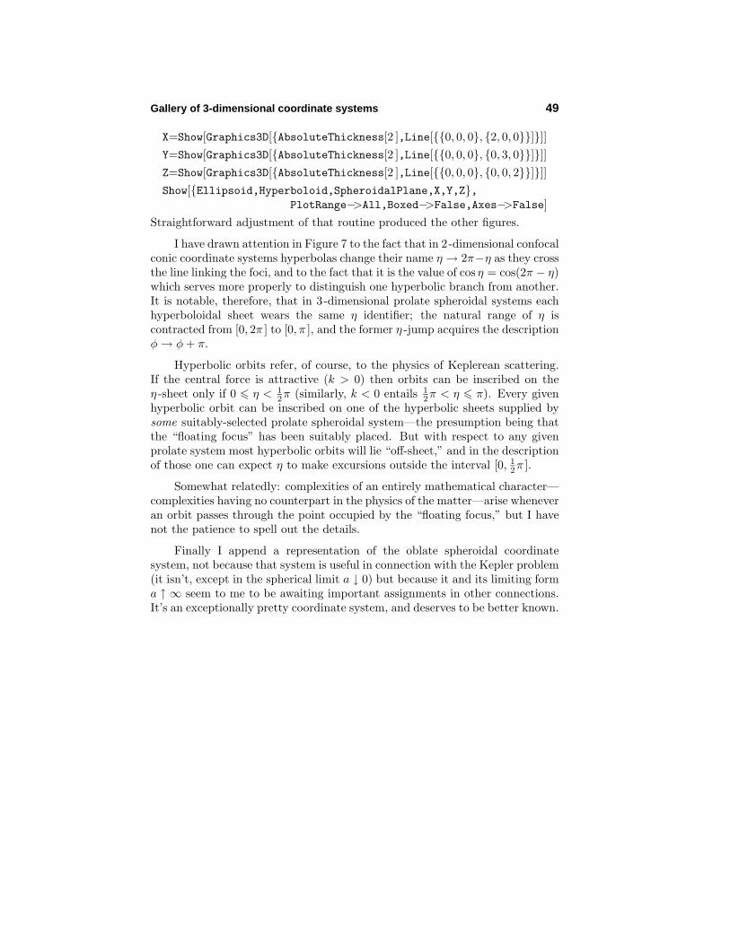
11. Graphical display of some 3-dimensional coordinate systems. It is in aneffort to make quite clear what we are talking about, and to lend visual variety tothe presentation, that I insert here three figures representative of the coordinatesystems which have recently generated so many equations. For the benefit ofreaders who may wish to engage in a bit of graphical experimentation (whichI encourage—not least because the colored display is so pretty) I reproducehere the Mathematica code which produced Figure 10: after a precautionaryClearAll writex[ξ , η , φ ] :=Cosh[ ξ ]Cos[ η ]−1y[ξ , η , φ ] :=Sinh[ ξ ]Sin[ η ]Cos[φ ]z[ξ , η , φ ] :=Sinh[ ξ ]Sin[ η ]Sin[φ ]Ellipsoid=ParametricPlot3D[x[1, η, φ ],−y[1, η, φ ], z[1, η, φ ],
η, 0, π, φ, π2 , 2π]Hyperboloid=ParametricPlot3D[x[ξ, 3
4 , φ ],−y[ξ, 34 , φ ], z[ξ, 3
4 , φ ],ξ, 0, 3
2, φ, π2 , 2π]SpheroidalPlane=ParametricPlot3D[x[ξ, η, π ],−y[ξ, η, π ], z[ξ, η, π ],
ξ, 0, 32, η, 0, π]
30 Born draws here upon work done by Pauli and—independently—byK. F. Niessen in , and is content to be sketchy because that work producednumbers which we found to be in disagreement with H+
2 data.31 Birtwhistle provides reference to Jacobi’s Vorlesungen uber Dynamik ,
p. 202, which might be the place to launch a serach of the literature.
46 Kepler problem in elliptical coordinates
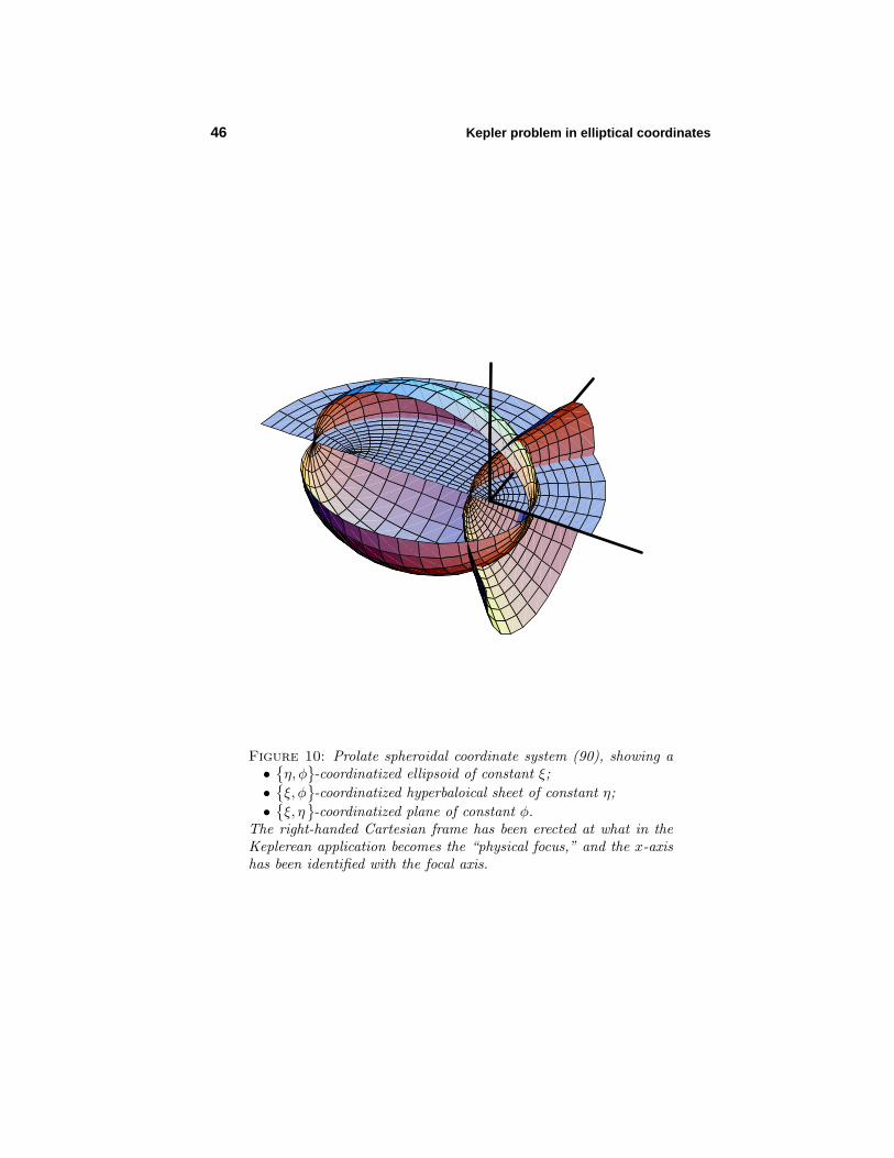
Figure 10: Prolate spheroidal coordinate system (90), showing a•
η, φ
-coordinatized ellipsoid of constant ξ;
•ξ, φ
-coordinatized hyperbaloical sheet of constant η;
•ξ, η
-coordinatized plane of constant φ.
The right-handed Cartesian frame has been erected at what in theKeplerean application becomes the “physical focus,” and the x-axishas been identified with the focal axis.
Gallery of 3-dimensional coordinate systems 47
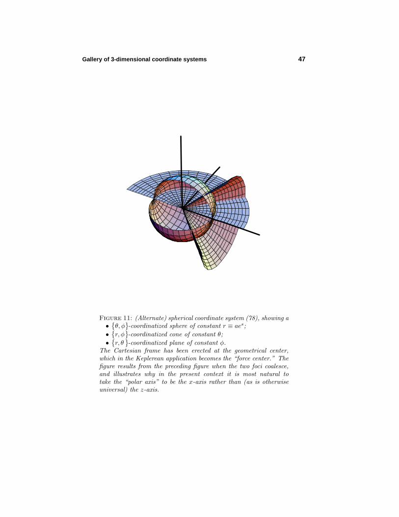
Figure 11: (Alternate) spherical coordinate system (78), showing a•
θ, φ
-coordinatized sphere of constant r ≡ aes;
•r, φ
-coordinatized cone of constant θ;
•r, θ
-coordinatized plane of constant φ.
The Cartesian frame has been erected at the geometrical center,which in the Keplerean application becomes the “force center.” Thefigure results from the preceding figure when the two foci coalesce,and illustrates why in the present context it is most natural totake the “polar axis” to be the x-axis rather than (as is otherwiseuniversal) the z-axis.

48 Kepler problem in elliptical coordinates
Figure 12: Parabolic coordinate system (85), showing a•
ν, φ
-coordinatized paraboloid of constant µ (opens left);
•µ, φ
-coordinatized paraboloid of constant ν (opens right);
•µ, ν
-coordinatized plane of constant φ.
The Cartesian frame has been erected at the shared focus, whichin the Keplerean application becomes the “force center.” The figureresults from Figure 10 when the “floating focus” is allowed to retreatto x→ −∞.
Gallery of 3-dimensional coordinate systems 49
X=Show[Graphics3D[AbsoluteThickness[2 ],Line[0, 0, 0, 2, 0, 0]]]Y=Show[Graphics3D[AbsoluteThickness[2 ],Line[0, 0, 0, 0, 3, 0]]]Z=Show[Graphics3D[AbsoluteThickness[2 ],Line[0, 0, 0, 0, 0, 2]]]Show[Ellipsoid,Hyperboloid,SpheroidalPlane,X,Y,Z,
PlotRange−>All,Boxed−>False,Axes−>False]Straightforward adjustment of that routine produced the other figures.
I have drawn attention in Figure 7 to the fact that in 2-dimensional confocalconic coordinate systems hyperbolas change their name η → 2π−η as they crossthe line linking the foci, and to the fact that it is the value of cos η = cos(2π − η)which serves more properly to distinguish one hyperbolic branch from another.It is notable, therefore, that in 3-dimensional prolate spheroidal systems eachhyperboloidal sheet wears the same η identifier; the natural range of η iscontracted from [0, 2π ] to [0, π ], and the former η -jump acquires the descriptionφ→ φ + π.
Hyperbolic orbits refer, of course, to the physics of Keplerean scattering.If the central force is attractive (k > 0) then orbits can be inscribed on theη -sheet only if 0 η < 1
2π (similarly, k < 0 entails 12π < η π). Every given
hyperbolic orbit can be inscribed on one of the hyperbolic sheets supplied bysome suitably-selected prolate spheroidal system—the presumption being thatthe “floating focus” has been suitably placed. But with respect to any givenprolate system most hyperbolic orbits will lie “off-sheet,” and in the descriptionof those one can expect η to make excursions outside the interval [0, 1
2π ].
Somewhat relatedly: complexities of an entirely mathematical character—complexities having no counterpart in the physics of the matter—arise wheneveran orbit passes through the point occupied by the “floating focus,” but I havenot the patience to spell out the details.
Finally I append a representation of the oblate spheroidal coordinatesystem, not because that system is useful in connection with the Kepler problem(it isn’t, except in the spherical limit a ↓ 0) but because it and its limiting forma ↑ ∞ seem to me to be awaiting important assignments in other connections.It’s an exceptionally pretty coordinate system, and deserves to be better known.
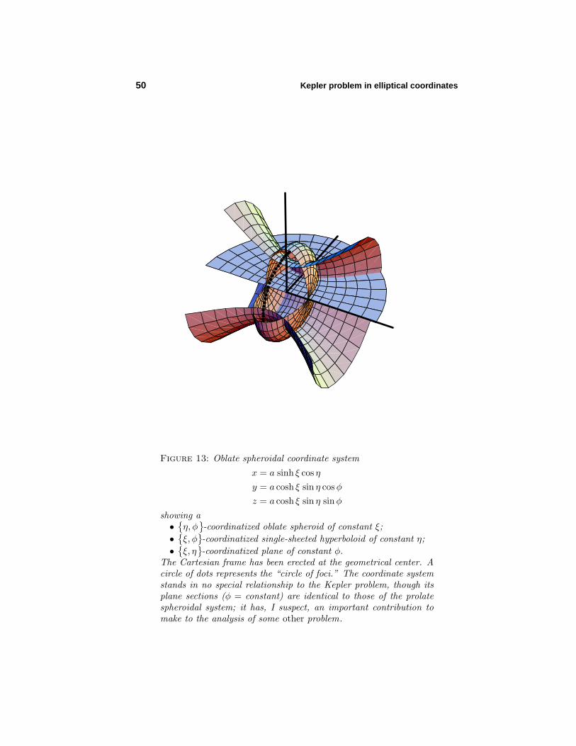
50 Kepler problem in elliptical coordinates
Figure 13: Oblate spheroidal coordinate system
x = a sinh ξ cos ηy = a cosh ξ sin η cosφz = a cosh ξ sin η sinφ
showing a•
η, φ
-coordinatized oblate spheroid of constant ξ;
•ξ, φ
-coordinatized single-sheeted hyperboloid of constant η;
•ξ, η
-coordinatized plane of constant φ.
The Cartesian frame has been erected at the geometrical center. Acircle of dots represents the “circle of foci.” The coordinate systemstands in no special relationship to the Kepler problem, though itsplane sections (φ = constant) are identical to those of the prolatespheroidal system; it has, I suspect, an important contribution tomake to the analysis of some other problem.

Universal Hamilton-Jacobi separability of Liouville’s systems 51
12. Universal Hamilton-Jacobi separability of Liouville’s systems. We have seenby example that separability of the Hamilton-Jacobi equation does not presumeseparability in the sense of Liouville. I digress now to demonstrate that, on theother hand, systems of Liouville’s design do universally give rise to separableHamilton-Jacobi equations.
Lagrangians of the form
L = 12
[v1(q1)q
21 + · · ·+ vn(qn)q2
n
]−
[w1(q1) + · · ·+ wn(qn)
]lead trivially to uncoupled equations of motion. Liouville () exploredimplications of the less restrictive assumption
L = 12u
[v1(q1)q
21 + · · ·+ vn(qn)q2
n
]−
[w1(q1) + · · ·+ wn(qn)
]u
u ≡ u1(q1) + · · ·+ un(qn)
which by a change of variable32 is tantamount to an assumption that theLagrangian possesses what I have called “Liouville’s design”33
L = 12u
[q21 + · · ·+ q2
n
]−
[w1(q1) + · · ·+ wn(qn)
]u
u ≡ u1(q1) + · · ·+ un(qn)
(93)
From p1 = uq1, . . . , pn = uqn we are led to a Hamiltonian of the correspondinglydistinctive but even simpler design
H = 1u
12
[p21 + · · ·+ p2
n
]+
[w1(q1) + · · ·+ wn(qn)
](94)
The associated time-independent Hamilton-Jacobi equation
12
[(∂S∂q1
)2 + · · ·+(∂S∂qn
)2] +[w1(q1) + · · ·+ wn(qn)
]= E u (95)
immediately separates on strength of the assumption
S(q1, . . . , qn) = S1(q1) + · · ·+ Sn(qn)
to yield the following uncoupled system of ordinary differential equations
12
(dS1dq1
)2 +[w1(q1 )− E u1(q1 )
]= ε1
12
(dS2dq2
)2 +[w2(q2 )− E u2(q2 )
]= ε2
...12
(dSn
dqn
)2 +[wn(qn)− E un(qn)
]= εn
(96)
32 See §43 in E. T. Whittaker’s Analytical Dynamics () for all missingdetails.
33 Notice that Liouville’s design requires the variables q to be co-dimensional.
52 Kepler problem in elliptical coordinates
where the (necessarily co-dimensional) separation constantsε1, ε2, . . . , εn
are
subject necessarily to the following constraint:
ε1 + ε2 + · · ·+ εn = 0 (97)
The “universal separability” to which my section title refers is thus established;what follows is by nature commentary.
Liouville himself, by Whittaker’s account, was interested not in separationof the Hamilton-Jacobi equation but in decoupling the equations of motion—which he did not quite accomplish (except in a familiar special case). By cleveranalysis34 he proceeded from the Lagrange equations implicit in (93) to a systemof first-order differential equations
12u
2 · q21 +
[w1(q1 )− E u1(q1 )
]= ε1
12u
2 · q22 +
[w2(q2 )− E u2(q2 )
]= ε2...
12u
2 · q2n +
[wn(qn)− E un(qn)
]= εn
(98)
which by u · qk = pk = ∂S∂q
k= ∂Sk
∂qk
are in fact precisely equivalent to (96).But while the system (96) is assuredly/universally separated, the system (98)becomes uncoupled only in the case u = constant, and in that case the Lagrangeequations latent in (93) are automatically uncoupled: Liouville can in that caseclaim simply to have reduced the order of the system.
In the case n = 2 Liouville eliminates the offending u2 term by dividingone equation—actually its square root—into the other; that procedure servesto eliminate not only the offending u -factor but also all reference to motion!One obtains an equation of the form
dq1dq2
=
√E · u1(q1)− w1(q1)− ε
E · u2(q2)− w2(q2) + ε
which we first encountered at (25), an equation which refers through q1(q2) tothe design of the orbit ; information relating to rate of progress along that orbithas then to be extracted from energy conservation by a separate argument. Inhigher-dimensional cases one might write
qi = qi(qn) : i = 1, 2, . . . , n− 1
and proceed similarly. . . into the higher reaches of analytical intractability.
A paraphrase of Liouville’s analysis could be erected upon the baseprovided by the canonical equations latent in (94)
q1 = 1up1 p1 = 1
u
[Hu′
1 − w′1
]u1
q2 = 1up2 p2 = 1
u
[Hu′
2 − w′2
]u2...
...qn = 1
upn pn = 1u
[Hu′
n − w′n
]un
34 See Whittaker, or §3 in Reference 1.
Universal Hamilton-Jacobi separability of Liouville’s systems 53
but I will not belabor the details.
Supposeq1, q2, q3
refer—relative to an inertial Cartesian frame—to a
locally orthogonal coordinatization of physical 3-space:
(dσ)2 ≡ (dx)2 + (dy)2 + (dz)2 = g1(dq1)2 + g2(dq2)
2 + g3(dq3)2
ThenL = 1
2m[x2 + y2 + z2
]− V (x, y, z)
= 12m
[g1q
21 + g2q
22 + g3q
23
]− U(q1, q2, q3)
will possess Liouville’s design if an only if
g1 = g2 = g3 = u(q1, q2, q3) ≡ u1(q1) + u2(q2) + u3(q3) (99.1)
and (simultaneously) the potential energy function has acquired the structure
U(q1, q2, q3) =w1(q1) + w2(q2) + w3(q3)
u(q1, q2, q3)(99.2)
In the 3-dimensional coordinate systems in which we have acquired interest onehas35
spherical : (dσ)2 = (dr)2 + r2(dθ)2 + r2 sin2 θ(dφ)2
alternate spherical : (dσ)2 = a2e2s[(ds)2 + (dθ)2
]+ a2e2s sin2 θ(dφ)2
parabolic : (dσ)2 = (µ2 + ν2)[(dµ)2 + (dν)2
]+ µ2ν2(dφ)2
prolate spheroidal : (dσ)2 = a2(cosh2 ξ + cos2 η)[(dξ)2 + (dη)2
]+ a2 sinh2 ξ sin2 η(dφ)2
—none of which satisfy condition (99.1); Hamilton-Jacobi separability in thosecases is (as previously noted) “non-Liouvillian.” But if one extinguishes thethird dimension (dφ = 0) then all but the spherical (polar) system conforms to(99.1), and (as we have seen) the Keplerean potential conforms also to (99.2); inthose cases separability “on the orbital plane” can be said to be “Liouvillian.”Some the preceding details will acquire new interest when, in connection withseparation of the Keplerean Schrodinger equation, we undertake to constructcurvilinear generalizations of ∇2.
On several occasions subsequent to (37) we were able to obtain valuableinformation by the simple expedient of “promoting Liouville’s separationconstant to the status of an observable.” I explore now the higher-dimensionalramifications of that idea, which—working from (96)—becomes
ε1 → G1 ≡ 12p
21 +
[w1 (q1 )−H u1 (q1 )
]ε2 → G2 ≡ 1
2p22 +
[w2 (q2 )−H u2 (q2 )
]...
εn → Gn ≡ 12p
2n +
[wn(qn )−H un(qn )
]
(100)
35 I take my information from Moon & Spencer.
54 Kepler problem in elliptical coordinates
where H was described at (94). I will, as a matter of expository convenience,henceforth set n = 3. The point transformation
x, y, z−→
q1, q2, q3
sends T = 1
2m[x2 + y2 + z2
]−→ u
[q21 + q2
2 + q23
], and in doing so induces the
“extended point transformation”x, y, z; px, py, pz
−→
q1, q2, q3; p1, p2, p3
Since such transformations are necessarily canonical, it becomes a matter ofindifference whether we use Cartesian or curvilinear variables when computingPoisson brackets, and—since it was in terms of the latter that the observablesG presented themselves at (100)—it proves more natural to use curvilinearcoordinates. With the (heroic!) assistance of Mathematica we quickly compute
[H,G1] = [H,G2] = [H,G3] = 0 (101)
and verify thatG1 + G2 + G3 = 0 (102)
Moreover[G1, G2] = [G1, G3] = [G2, G3] = 0 (103)
We expect these results to sustain 3→ n generalization; I have not attemptedto construct a formal proof, but will proceed as though such a proof were inhand.
I know of no “natural” way to select or assemble n−1 objects from n, so dothe obvious simple (but symmetry-breaking) thing: I select
G1, G2, . . . , Gn−1
and understand Gn to be recoverable from Gn = −(G1 + G2 + · · · + Gn−1).The set
H,G1, G2, . . . , Gn−1
is a set of n observables, each of which (in the
Poisson bracket sense) commutes with every other; the set is, in other words,involutory (its elements are “in involution”), with powerful consequences (somedue to Liouville himself) which are detailed in Whittaker’s §§147 & 148.36
It is a notable fact that the conserved observables Gi supplied by (100)are of non-Noetherean design. The substance of this remark has been detailedelsewhere,37 but its deeper meaning and ultimate consequences I do not yetunderstand.
In the case n = 2 we are at (100) supplied with only a single observable,namely
G1 ≡ 12p
21 +
[w1(q1)−H u1(q1)
](104)
36 In quantum mechanics such maximal involutory sets become “completesets of simultaneous (or commuting) observables.”
37 See §4 in Reference 1. In essence, the observables J supplied by Noether’stheorem acquire their quadratic p -dependence entirely from the Hamiltonian,which enters as a factor, but the observables G generally exhibit also some“dangling p -dependence.”

Curvilinear quantization 55
which on its face does not much resemble either −G2 or the G which at (37)was obtained by an “E-elimination procedure” and gave rise ultimately to (42).But when written out in explicit detail, (104) reads
G1 =
[u2(q2)p
21 − u1(q1)p
22
]+ 2
[u2(q2)w1(q1)− u1(q1)w2(q2)
]2[u1(q1) + u2(q2)
]which clearly does conform to (102)
G1 + G2 = 0
and clearly does mimic the design of (37).I bring this discussion to an arbitrary end with some brief historical and
bibliographic remarks. Whittaker concludes his §43 with reference to the“further investigations on this subject” by P. Stackel (), J. Hadamard(), P. Burgatti () and V. S. Vrkljan (). From the more detailedreferences to the work of Stackel38 supplied by Moon & Spencer it becomesapparent that Stackel drew his motivation directly from Hamilton-Jacobi theory(not from the theory of partial differential equations in some more generalizedsense), while the references to Stackel which Goldstein introduced into hissecond edition (see especially p. 453 and Appendix D) make it abundantly clearthat Stackel took Liouville’s work as his specific point of departure.39
PART III: SCHRODINGER THEORY
13. Escape from Cartesian tyranny: curvilinear quantization. Though Newton’screative fire took its energy from sources which will always remain somewhatwrapped in mystery, it is clear that he worked always in reaction to themetaphysics of Rene Descartes, and it becomes therefore one of the ironiesof history that his first act in the Principia () was to attach a Cartesianframe to the fixed stars, and thus to place mechanics under the thumb of akind of “Cartesian tyranny.” Autocratic regimes may simplify life, but providelimited opportunity, and have ultimately to be cast off. Which may take awhile.In mechanics the escape from Cartesian tyranny—of which
FFF = mxxx −→ddt
∂∂q− ∂
∂q
L = 0
38 “Uber die Integration der Hamilton-Jacobischen Differentialgleichungmittels Separation der Variabelen” (); “Sur une classe de problemes dedynamique” (); “Uber die Integration der Hamiltonschen Differential-gleichung mittels Separation der Variabelen” ().
39 The Dictionary of Scientific Biography accords Paul Stackel (–)only brief notice: we are informed that he was a disciple of Weierstrass, taughtat Heidelberg, specialized in analytical mechanics and related geometry, thetheory of analytic functions and (in later years) set theory and the theory ofprime numbers. He was also active as an historian of 18th and early 19th
Century science; he played a major role in arranging for publication of Euler’sOpera omnia and also edited works of (among others) Gauss and Jacobi.
56 Kepler problem in elliptical coordinates
provides a cartoon—took the better part of a century, and became completeonly with the publication () of Lagrange’s Mechanique analytique.
Quantum mechanics admits of famously many distinct but equivalentformulations, of which some are better known than others, but all (or almostall—certainly all of the standard formulations) were created by, and are todaycultivated by, physicists seemingly content to go about their practical worksubject to the strictures of a benign Cartesian tyranny. Of present interest tome is the formalism formerly known as “wave mechanics,” but which I now findit convenient to call “Schrodinger theory.” Within that formalism one proceeds
Hamiltonian∣∣Cartesian
−−−−−−−−→ Hamiltonian∣∣curvilinear
|| p→
i∂∂x|↓
Schrodinger∣∣Cartesian
−−−−−−−−→ Schrodinger∣∣curvilinear
and the subtle presence of Cartesian tyranny (or is it merely chauvinism?) isrevealed the absence of a descending arrow on the right. Such an arrow canbe installed, but it takes some doing.40 But since it leads to a result which (atleast in flat space) is not in dispute, I will—with explicit acknowledgement thatI am doing so—be content on this occasion to join the masses in acquiescing tothe now-traditional tyranny.
So we take −
2
2m∇2− k 1√
x2+y2+z2
ψ = Eψ (105)
as our point of departure, and recall that if curvilinear coordinatesq1, q2, q3
are introduced by equations of the form
x = x(q1, q2, q3)
y = y(q1, q2, q3)
z = z(q1, q2, q3)
then(ds)2 ≡ (dx)2 + (dy)2 + (dz)2 = gij(q)dqidqj
40 One must recognize first of all that the wave function ψ(xxx) transforms notas a scalar field, but as a scalar density of weight W = 1
2 . One must recognizealso that (and how) Laplace-Beltrami operators ∇2(W ) appropriate to scalardensities are to be distinguished from the (more familiar) operators ∇2 ≡ ∇2(0)appropriate to simple scalars. One then finds that the quantization procedureppp→
i∇∇∇ has in general to be described
ppp −→ covariant derivative operator of weight W = 12
For an elaborate account of the details (the overthrow of tyranny sometimescalls for terrorism) see quantum mechanics (), Chapter 2, pp. 153–183.
Curvilinear quantization 57
where the metric matrix ‖gij‖ is everywhere diagonal if the q-system is(everywhere locally) orthogonal. In all events one has
∇2 = 1√g∂∂qi
√ggij ∂
∂qj
(here ‖gij‖ ≡ ‖gij‖–1 and g ≡ det ‖gij‖) which in orthogonal cases simplifies:
∇2 = 1√g
∂∂q1√gg11 ∂
∂q1 + 1√g
∂∂q2√gg22 ∂
∂q2 + 1√g
∂∂q3√gg33 ∂
∂q3
And since
‖gij‖ =
g1 0 0
0 g2 00 0 g3
entails g = g1g2g3 and ‖gij‖ =
g–1
1 0 00 g–1
2 00 0 g–1
3
we have
∇2 = 1√g1g2g3
∂∂q1
√g2g3g1
∂∂q1 + ∂
∂q2
√g1g3g2
∂∂q2 + ∂
∂q3
√g1g2g3
∂∂q3
so, taking our metric data from equations displayed just prior to (100), weobtain
∇2Cartesian =
(∂∂x
)2 +(∂∂y
)2 +(∂∂z
)2 (106.1)
∇2spherical = 1
r2 sin θ
∂∂r r
2 sin θ ∂∂r + ∂
∂θ sin θ ∂∂θ + ∂
∂φ1
sin θ∂∂φ
(106.2)
∇2alternate = 1
a3e3s sin θ
∂∂sae
s sin θ ∂∂s + ∂
∂θaes sin θ ∂
∂θ
+ ∂∂φ
aes
sin θ∂∂φ
(106.3)
∇2parabolic = 1
µν(µ2+ν2)
∂∂µµν
∂∂µ + ∂
∂νµν∂∂ν + ∂
∂φµ2+ν2
µν∂∂φ
(106.4)
∇2displaced spheroidal = 1
a3 sinh ξ sin η(sinh2 ξ+sin2 η)
∂∂ξa sinh ξ sin η ∂
∂ξ
+ ∂∂ηa sinh ξ sin η ∂
∂η + ∂∂φ
sinh2 ξ+sin2 ηsinh ξ sin η
∂∂φ
(106.5)
The Kepler problem requires us to recall also these implications√x2 + y2 + z2 = r
= aes
= 12 (µ2 + ν2)
= a(cosh ξ − cos η)
of the coordinate definitions (71),(78), (85) and (90), and in connection with(106.5) it proves useful to notice that sinh2 ξ + sin2 η = cosh2 ξ − cos2 η.
Pull-back to the orbital plane—identified with thex, y
-plane—leaves the
classical physics (though not the classical Hamilton-Jacobi physics) of central
58 Kepler problem in elliptical coordinates
force problems unaffected, but is profoundly unphysical in quantum mechanics,where it becomes a merely formal exercise. But informative, for that veryreason. In preparation for such exercise we use
∇2 = 1√g1g2
∂∂q1
√g2g1
∂∂q1 + ∂
∂q2
√g1g2
∂∂q2
(107)
to obtain
∇2Cartesian =
(∂∂x
)2+(∂∂y
)2 (108.1)
∇2polar = 1
r
∂∂r r
∂∂r + ∂
∂θ1r∂∂θ
(108.2)
∇2alternate = 1
a2e2s
(∂∂s
)2+(∂∂θ
)2
(108.3)
∇2parabolic = 1
µ2+ν2
(∂∂µ
)2+(∂∂ν
)2
(108.4)
∇2displaced conic = 1
a2(sinh2 ξ+sin2 η)
(∂∂ξ
)2+(∂∂η
)2
(108.5)
Note how non-trivial is the procedure by which (107) is extracted from its3-dimensional counterpart; i.e., by which (106) → (108). And how especiallysimple (except in the polar case) are the latter equations. That simplicityis a direct reflection of the circumstance that the metric is in those cases“conformally Euclidean”
‖gij‖ = u ·(
1 00 1
)and endowed therefore with the specialized structure assumed by Liouville.
Chapter 21 of Abramowitz & Stegun’s Handbook of Mathematical Functionsprovides a valuable account of “Spheroidal Wave Functions,” but proceeds fromdefinitions of the associated prolate/oblate coordinate systems which departfrom my own conventions. In essence, where I (at the beginning of §9) wrote
x = a cosh ξ cos ηy = a sinh ξ sin η cosφz = a sinh ξ sin η sinφ
they would write (but without the hats)
x = aξ η
y = a
√(ξ2 − 1)(1− η2) cosφ
z = a
√(ξ2 − 1)(1− η2) sinφ
and in place of our “displaced” system (90) they would write
x = aξ η − a
y = a
√(ξ2 − 1)(1− η2) cosφ
z = a
√(ξ2 − 1)(1− η2) sinφ
(109)
Spherical separation of the Schrodinger equation 59
One in either case (with or without displacement) computes
(ds)2 = a2 ξ2−η2
ξ2−1(dξ)2 + a2 ξ2−η2
1 −η2 (dη)2 + a2(ξ2 − 1)(1− η2)(dφ)2
giving
∇2 = 1a3(ξ2−η2)
∂∂ξ
a(ξ2 − 1) ∂∂ξ
+ ∂∂η a(1− η2) ∂
∂η
+ ∂∂φa
ξ2−η2
(ξ2−1)(1−η2)∂∂φ
(110)
“Displacement” does, however, serve to simplify the description of
r =√
x2 + y2 + z2 =
a(ξ − η) with displacementa√
ξ2 + η2 − 1 without
Pull-back to thex, y
-plane is accomplished by setting sinφ = 0 in (109); we
then compute(ds)2 = a2 ξ2−η2
ξ2−1(dξ)2 + a2 ξ2−η2
1 −η2 (dη)2 (111)
and notice thatξ, η
→
ξ, η
has caused the metric to lose its formerly
conformal structure, with the consequence that the descriptioin of ∇2 loses itsformer simplicity:
∇2 =√
(ξ2−1)(1−η2)
a2(ξ2−η2)
∂∂ξ
[ξ2−11 −η2
]+ 12 ∂∂ξ
+ ∂∂η
[ξ2−11 −η2
]− 12 ∂∂η
(112)
We have previously had occasion to notice thatr, θ
s, θ
entails both
costs and benefits: the former system serves well the purposes of analysis (whenexpanded to include φ it supports the standard formulation of the theory ofspherical harmonics) but only the latter serves the specialized needs of Liouville.The situation with regard to
ξ, η
ξ, η
is similar.
14. Spherical separation of the Schrodinger equation. Returning with (106.2)to (105), we have
− 2
2m
[1r2
∂∂r r
2 ∂∂r + 1
r2
1
sin θ∂∂θ sin θ ∂
∂θ + 1sin2 θ
(∂∂φ
)2]− k
r
ψ = Eψ
after simplifications. Separation proceeds from the assumption (compare (74))that the wave function has the factored design
ψ(r, θ, φ) = R(r)·Θ(θ)· Φ(φ) (113)
An initial separation gives1r2
ddr r
2 ddr + 2m
2
[E + k
r
]− λ
r2
R(r) = 0 (114.1)
1sin θ
∂∂θ sin θ ∂
∂θ + 1sin2 θ
(∂∂φ
)2Y (θ, φ) = −λ · Y (θ, φ) (114.2)
60 Kepler problem in elliptical coordinates
where λ is a spearation constant and Y (θ, φ) ≡ Θ(θ) · Φ(φ). Allusion to theCoulomb potential is confined to the “radial equation (114.1); to say the samething another way. . .
The angular equation (114.2) contains no reference to the force strengthk, and arises whatever the central potential U(r). It refers to the rotationalsymmetry of such problems, and gives rise to the familiar theory of “sphericalharmonics,” which is but another name for the “quantum theory of angularmomentum.” To summarize the highlights of that well known subject, treatedin every text:41 physically acceptable solutions of (114.2) are found to arise ifan only if λ = ( + 1) with ∈
0, 1, 2, . . .
, and are found to be of the form
Y m (θ, φ) = (normalization factor) · eimφPm
(cos θ) (115)
where m ∈− , . . . ,+
and the normalization factor is designed to achieve
orthonormality on the sphere:∫ 2π
0
∫ π
0
Y m (θ, φ)Y m′
′ (θ, φ) sin θ dθdφ = δ′δmm′
Contact with the theory of angular momentum is made explicit by the equations
L2 Y m = ( + 1)2 · Y m
and LpolarYm = m · Y m
(116)
(Here I have written Lpolar where one expects to see Lz because, though it isconventional to identify the z -axis with the polar axis of the spherical coordinatesystem, I have found it more natural to assign that distinction to the x-axis; thenotation Lpolar is intended to capture the essence of the matter in a convention-independent way.) Finally, if R is a rotation matrix then
xxx→ xxx = Rxxx induces Y m → Y m
=n=+∑n=−
Rmn()Y n
where ‖Rmn()‖ provides a (2+1)×(2+1)-dimensional matrix representation
of the action of O(3).
Turning now to the radial equation (114.1)—where λ = (+1) has now tobe understood—one might expect, after imposition of physical side conditions,to have
− 2
2m1r2
ddr r
2 ddr − k
r + 2
2m(+1)r2
R(r) = E()R(r) (117)
with
degeneracy of En() = 2 + 1 : number of Y m with the given
41 I particularly like the uncluttered discussion to be found in Chapter 7 ofJ. Powell & B. Crassman, Quantum Mechanics (). See also my “Algebraictheory of spherical harmonics” ().
Spherical separation of the Schrodinger equation 61
and that is indeed the situation typical of arbitrary central potentials U(r).But the case U(r) = −k/r is special: it emerges in that case that if we agreeto write
En()≡ spectral set associated with case
then En()
⊂
En(− 1)
⊂ · · · ⊂
En(0)
on which basis we anticipate that
E1 is 1-fold degenerateE2 is 1 + 3 = 22-fold degenerateE3 is 1 + 3 + 5 = 32-fold degenerate...
En is 1 + 3 + · · ·+ (2n− 1) = n2-fold degenerate
I have alluded here to facts—illustrated in Figure 14—usually obtained byexplicit solution of the radial equation;42 one finds that (117) possessesphysically acceptable (bound state) solutions if and only if
E() = Eν, ≡ −E01
(ν++1)2 : ν = , + 1, + 2, . . . (118)
E0 ≡ mk2
22
and that in those cases
R(r) = (normalization factor) · e− 12xx
α−12 Lα
ν (x) (119)
where α ≡ 2 + 1 and x ≡ 2ν++1 (r/a0) with a0 ≡
2/mk = “Bohr radius.”One is motivated by the structure of these results to introduce the so-called“principal quantum number”
n = n(ν, ) ≡ ν + + 1 : n = 1, 2, 3, . . . (120)
in terms of which one has radial eigenfunctions
Rn(r) = (normalization factor) · e−r/na0(2r/na0)L2+1n−−1(2r/na0) (121)
and associated eigenvalues with depend upon n and not individually but onlyin the combination n(ν, )
En = −E01n2 (122)
It is this fact—degeneracy over and above the m-independence which arises fromrotational symmetry—to which the phrase “accidental degeneracy” refers. We
42 See, for example, Schiff (Reference 59, §16) for a good account of thetedious details.
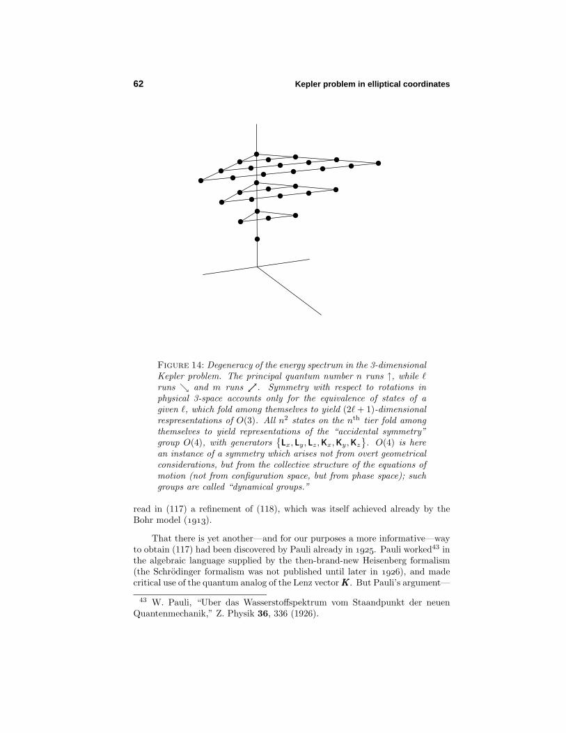
62 Kepler problem in elliptical coordinates
Figure 14: Degeneracy of the energy spectrum in the 3-dimensionalKepler problem. The principal quantum number n runs ↑, while runs and m runs . Symmetry with respect to rotations inphysical 3-space accounts only for the equivalence of states of agiven , which fold among themselves to yield (2 + 1)-dimensionalrespresentations of O(3). All n2 states on the nth tier fold amongthemselves to yield representations of the “accidental symmetry”group O(4), with generators
Lx, Ly, Lz,Kx,Ky,Kz
. O(4) is here
an instance of a symmetry which arises not from overt geometricalconsiderations, but from the collective structure of the equations ofmotion (not from configuration space, but from phase space); suchgroups are called “dynamical groups.”
read in (117) a refinement of (118), which was itself achieved already by theBohr model ().
That there is yet another—and for our purposes a more informative—wayto obtain (117) had been discovered by Pauli already in . Pauli worked43 inthe algebraic language supplied by the then-brand-new Heisenberg formalism(the Schrodinger formalism was not published until later in ), and madecritical use of the quantum analog of the Lenz vector KKK. But Pauli’s argument—
43 W. Pauli, “Uber das Wasserstoffspektrum vom Staandpunkt der neuenQuantenmechanik,” Z. Physik 36, 336 (1926).
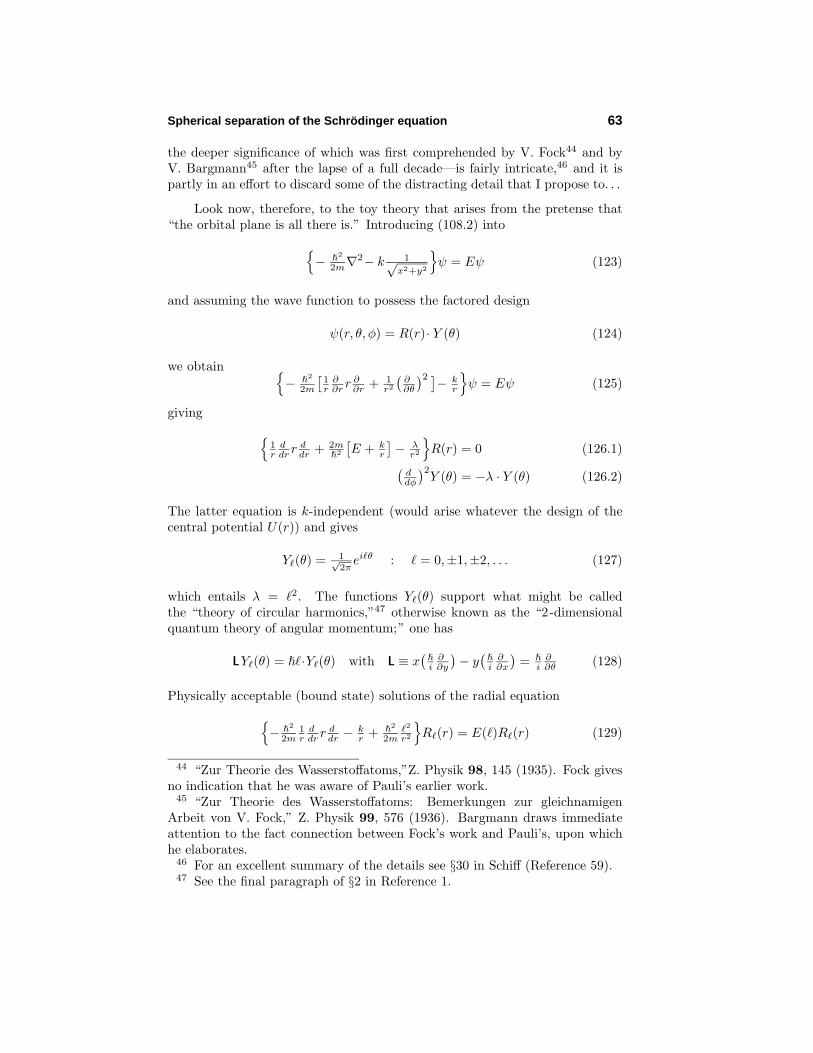
Spherical separation of the Schrodinger equation 63
the deeper significance of which was first comprehended by V. Fock44 and byV. Bargmann45 after the lapse of a full decade—is fairly intricate,46 and it ispartly in an effort to discard some of the distracting detail that I propose to. . .
Look now, therefore, to the toy theory that arises from the pretense that“the orbital plane is all there is.” Introducing (108.2) into
−
2
2m∇2− k 1√
x2+y2
ψ = Eψ (123)
and assuming the wave function to possess the factored design
ψ(r, θ, φ) = R(r)· Y (θ) (124)
we obtain −
2
2m
[1r∂∂r r
∂∂r + 1
r2
(∂∂θ
)2 ]− k
r
ψ = Eψ (125)
giving 1rddr r
ddr + 2m
2
[E + k
r
]− λ
r2
R(r) = 0 (126.1)(
ddφ
)2Y (θ) = −λ · Y (θ) (126.2)
The latter equation is k-independent (would arise whatever the design of thecentral potential U(r)) and gives
Y(θ) = 1√2π
eiθ : = 0,±1,±2, . . . (127)
which entails λ = 2. The functions Y(θ) support what might be calledthe “theory of circular harmonics,”47 otherwise known as the “2-dimensionalquantum theory of angular momentum;” one has
LY(θ) = ·Y(θ) with L ≡ x(
i∂∂y
)− y
(
i∂∂x
)=
i∂∂θ (128)
Physically acceptable (bound state) solutions of the radial equation
−
2
2m1rddr r
ddr − k
r + 2
2m2
r2
R(r) = E()R(r) (129)
44 “Zur Theorie des Wasserstoffatoms,”Z. Physik 98, 145 (1935). Fock givesno indication that he was aware of Pauli’s earlier work.
45 “Zur Theorie des Wasserstoffatoms: Bemerkungen zur gleichnamigenArbeit von V. Fock,” Z. Physik 99, 576 (1936). Bargmann draws immediateattention to the fact connection between Fock’s work and Pauli’s, upon whichhe elaborates.
46 For an excellent summary of the details see §30 in Schiff (Reference 59).47 See the final paragraph of §2 in Reference 1.

64 Kepler problem in elliptical coordinates
arise48 if and only if
E() = Eν, ≡ −E01
(ν+||+ 12 )2
: ν = ||, ||+ 1, ||+ 2, . . . (130)
and in those cases one has
R(r) = (normalization factor) · e− 12xx
α2 Lα
ν (x) (131)
where now α ≡ 2|| and x ≡ 2ν+||+ 1
2(r/a0), though E0 and a0 have retained
their former definitions. If one adopts this slight modification
n = n(ν, ) ≡ ν + ||+ 1 : n = 1, 2, 3, . . .
of our former definition of the “principal quantum number” then we are enabledto write
En = −E01
(n− 12 )2
= −4E01
(2n−1)2 (132)
and (compare (121))
Rn(r) = (normalization factor) · e− 12xx||L2||
n−||−1(x) (133)
where now x = 2n− 1
2(r/a0) = 4
2n−1 (r/a0).
We are in position now to take inventory of the consequences of dimensionalretraction
2-dimensions ←− 3-dimensions
The induced adjustment
circular harmonics Y(θ) ←− spherical harmonics Y m (θ, φ)
is profound but unproblematic. The adjustment
Rn(r) ∼ e−12xx||L2||
n−||−1(x) ←− Rn(r) ∼ e−12xxL2+1
n−−1(x)
seems function-theoretically modest on its face, but note: it presumes
x = 2n− 1
2(r/a0) ←− x = 2
n (r/a0)
which at n = 1 reads x = 4(r/a0)← x = 2(r/a0); the radial function Rn(r) hasbeen rendered spatially more compact . Which is a little surprising, for the Bohrmodel is effectively 2-dimensional, and it gives “orbits of the correct diameter”(by which we really mean only that it gives the observed spectroscopy). Thisdevelopment is consistent with
En = −E01
(n− 12 )2
←− En = −E01n2
according to which
Dimensional reduction depresses the energy spectrum
48 Here I borrow (except for misprints) from B. Zaslow & M. E. Zandler,“Two-dimensional analog to the hydrogen atom,” AJP 35, 1118 (1967).
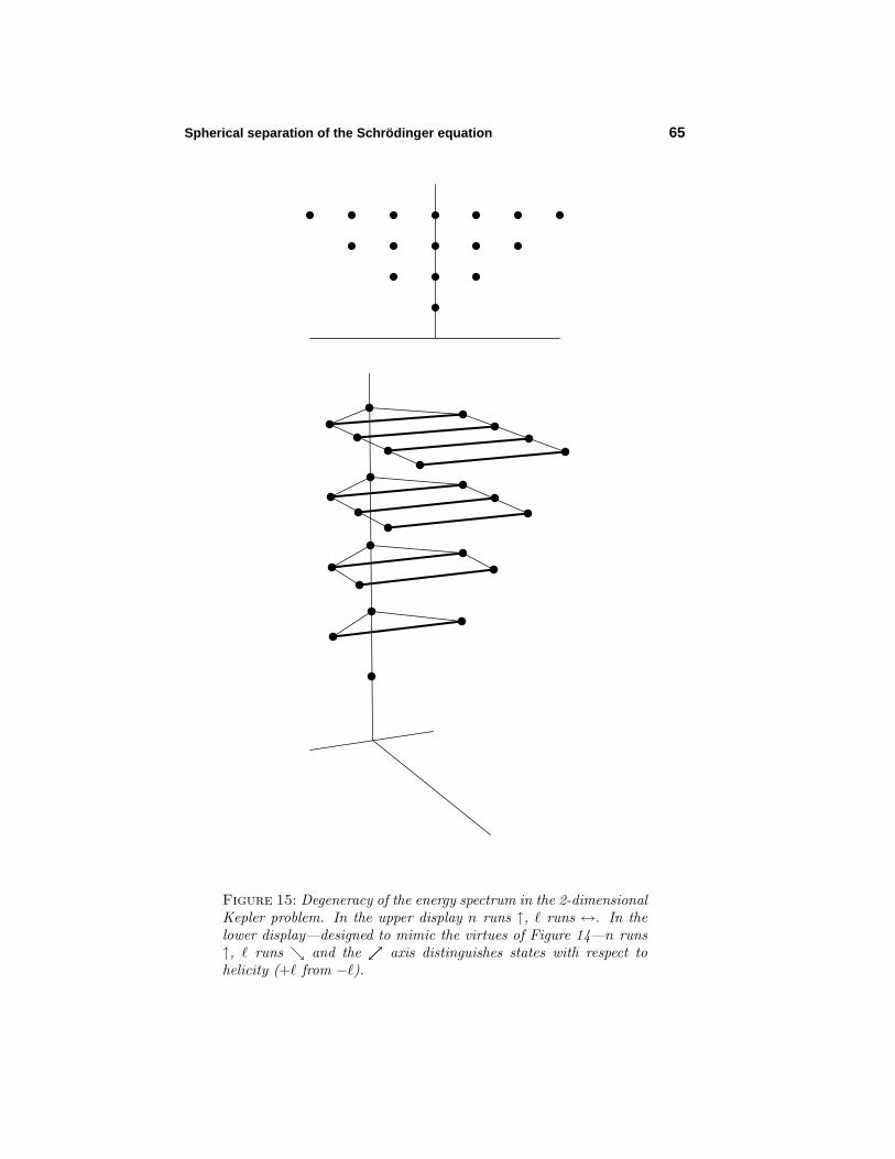
Spherical separation of the Schrodinger equation 65
Figure 15: Degeneracy of the energy spectrum in the 2-dimensionalKepler problem. In the upper display n runs ↑, runs ↔. In thelower display—designed to mimic the virtues of Figure 14—n runs↑, runs and the axis distinguishes states with respect tohelicity (+ from −).
66 Kepler problem in elliptical coordinates
Specifically, the ground state of the 2-dimensional hydrogen atom lies four timesdeeper than the ground state of the 3-dimensional atom. And according toR. Louden the trend continues; he reports49 that for 1-dimensional hydrogenE0 = −∞.50 Finally, dimensional reduction radically alters the degeneracystructure of the energy spectrum—from that shown in Figure 14 to that shownin Figure 15. More specifically, we have
degeneracy with respect to helicity(sign of ) is geometrical, but
degeneracy with respect is accidental
←
degeneracy with respect to mis geometrical, but
degeneracy with respect is accidental
which puts us in position at last to consider the. . .
15. 2-dimensional analog of Pauli’s argument. We have
H = 12m
[p2x + p2
y
]− k
[x2 + y2
]− 12 (134)
and at (128) acquired interest in
L = x py − y px (135)
With labor51 we confirm that
[ H, L ] = O (136)
With Pauli (who was content to borrow from Lenz52) we borrow from (38) thesehermitianized counterparts of Kx and Ky (Kz being of no present interest)
Kx ≡ + 12m
[pyL + L py
]− k x
[x2 + y2
]− 12
Ky ≡ − 12m
[pxL + L px
]− k y
[x2 + y2
]− 12
(137)
49 “One-dimensional hydrogen atom,” AJP 27, 649 (1959).50 Zaslow & Zandler remark that the boxed statement pertains also to
particle-in-a-box problems, and to oscillators. The question therefore arises:Can one show that holds generally? Such a result seemsintuitively plausible, but would be in one respect anomalous: for a particlein an a-by-b box one has
E0 = π22
2m
[1a2 + 1
b2
]which
grows as b ↓ 0, but
assumes a reduced value whenthe b -dimension is discarded
We touch here on this deep problem: How does one properly incorporateholonomically constrained coordinates into quantum theory?
51 I ask Mathematica to confirm that HLf(x, y) = LHf(x, y) for all f(x, y),with L = β(x∂y − y∂x), etc., β being a place holder for /i.
52 W. Lenz, “Uber den Bewegungsverlauf und die Quantenzustande dergestorten Keplerbewegung,” Z. Physik 24, 197 (1924). Lenz cites C. Runge’s
Hidden symmetry: 2-dimensional analog of Pauli’s argument 67
and at length establish the following commutation relations:
[ H,Kx ] = [ H,Ky ] = O (138)
[ Kx,Ky ] = −i 2mH L
[ Ky , L ] = +i Kx
[ L ,Kx ] = +i Ky
Within each eigenspace of H we can replace the operator by its eigenvalue E,which for bound states is negative. It makes sense, therefore, to introduce(compare (47.2))
J1 ≡ Kx
/√− 2
mE
J2 ≡ Ky
/√− 2
mE
J3 ≡ L
(139)
in terms of which we have [J1, J2
]= i J3[
J2, J3
]= i J1[
J3, J1
]= i J2
(140)
and therefore (immediately)[J2, J1
]=
[J2, J2
]=
[J2, J3
]= O with
J2 ≡ J21 + J2
2 + J23
= L2 − m2EK2 (141)
Classically
K2 ≡ K2x + K2
y =[
1mpy(xpy−ypx)− k
rx]2 +
[1mpx(ypx−xpy)− k
r y]2
= 2m
[1
2m (p2x + p2
y)− kr
][xpy − ypx
]2 + k2
= 2mHL2 + k2
so we are not surprised to discover by (heavy!) exploratory calculation that
K2 ≡ K2x + K2
y = 2mH ( L2 + 1
42I ) + k2 I (142)
Retreating now again to the (bound state) eigenspace HE ⊂ H, we have
[continued from the preceding page] Vektoranalysis () as his own source,and, according to Goldstein, Runge borrowed his material from Gibbs (∼).The Dictionary of Scientific Biography makes no mention of Lenz, but providesa fascinating account of the life of Carl Runge (–), who appears to havebeen introduced to his future wife, to have been motivated to move from puremathematics into spectral physics, and ultimately to have become the father-in-law of Richard Courant—all in consequence of having been tall, handsome,and an outstanding ice skater.
68 Kepler problem in elliptical coordinates
J2 = L2 − m2E
2mE ( L2 + 1
42I ) + k2 I
= −
[14
2 + mk2
2E
]I (143)
Borrowing from the algebraic formulation of the 3-dimensional quantum theoryof angular momentum53 we know that
J2 has eigenvalues j(j + 1)2 with j = 0, 12 , 1,
32 , 2, . . .
and thatthe eigenvalue j(j + 1)2 is (2j + 1)-fold degenerate
Bring this information to (143) we obtain
−mk2
2E =[j(j + 1) + 1
4
]
2
= 14 (2j + 1)2
2
giving
E(j) = −4mk2
221
(2j+1)2 (144)
= −4E01
(integer)2
Whether one argues analytically (with Schrodinger) or group-theoretically (withPauli), one has Bohr’s result
E = −E01
(integer)2 in the 3-dimensional case
while at (132) Zaslow & Zandler’s analytical argument yielded
E = −4E01
(odd integer)2 in the 2-dimensional case
with the implication that at (144) we must exclude the fractional values of j.With respect to description of the “hidden symmetry” of the 2-dimensionalhydrogen atom one must disallow the spinor representations of the rotationgroup; the “dynamical group” of that system is (we speak only of the boundstates) O(3), not SU(2).54
It is, in this light, more natural to assign to j the work formerly assignedto the principal quantum number n; the identification 2j + 1 = 2n− 1 entails
n = j + 1 : j = 0, 1, 2, . . .
so we acquire the notations
En = Ej+1 = E(j)
53 See, for example, Schiff’s §27, Mertzbacher’s Chapter 16, or §§4.3 & 4.4 inD. Griffiths’ Introduction to Quantum Mechanics ().
54 It is now easy to understand how confusion on this point might arise, ashistorically it did arise. For detailed discussion and references see A. Cisneros &H. V. McIntosh, “Symmetry of the two-dimensional hydrogen atom,” J. Math.Phys. 10, 277 (1969). I return to this problem on p. 77 below.
Hidden symmetry: 2-dimensional analog of Pauli’s argument 69
Turning now again to description (within the 2-dimensional theory) of thehydrogenic wavefunctions (i.e., to construction of a natural basis in HE(j)) weagain borrow from the 3-dimensional quantum theory of angular momentum,introducing
J+ ≡ J1 + iJ2 = ( Kx + iKy)√−m/2E(j)
J− ≡ J1 − iJ2 = ( Kx − iKy)√−m/2E(j)
(145)
From (140) it then follows that [J2, J±
]= O[
L, J±]
=[J3, J±
]= ± J±
(146)
The (non-hermitian) “ladder operators” ± are introduced because—as isestablished by an algebraic argument which it must have given immeasurablesatisfaction to its inventor, but which it would be pointless to reproduce—theypermit one to climb up and down through the set
|j, ) : = −j, . . . ,−1, 0,+1, . . . ,+j
of simultaneous eigenstates of J2 and L:
J2|j, ) = j(j + 1)2 |j, ) and L|j, ) = |j, )
In 3-dimensional physics one encounters operatorsLx, Ly, Lz
which are (as we
have had occasion already to remark) algebraically identical to the operatorsJx, Jy, Jz
of present interest. In that context the operators
L±, Lz, L
2
acquire representations
L± = ±e±iφ(∂∂θ ± i cot θ ∂
∂φ
)Lz =
i∂∂φ
L2 = L+L− + L2z − Lz
and the eigenstates |,m) become just the familiar spherical harmonics Y m (θ, φ).
The 2-dimensional Kepler problem gives rise, however, to quite a differentrealization of the same algebra. Introducing
x = r cos θy = r sin θ
px =
i
cos θ · ∂∂r − 1
r sin θ · ∂∂θ
py =
i
sin θ · ∂∂r + 1
r cos θ · ∂∂θ
(147)
into first (135) and then (137) we obtain
L =
i∂∂θ
K+ = eiθ[
2
2mr
(1− 2i ∂∂θ
)(r ∂∂r + i ∂∂θ
)+ k
]K− = complex conjugate of the above
(148)
70 Kepler problem in elliptical coordinates
and confirm by explicit calculaton that the operators thus described to in factsatisfy the anticipated commutation relations. With (148) in hand, we are inposition to construct polar representations of J2 and J±, though in this regardtwo interrelated points should be borne in mind:•Within the jth energy eigenspace HE(j) the action of J2 is almost trivial: if|ψ) ∈ HE(j) then J2|ψ) = j(j + 1)2|ψ);• The presence of the factor
√−m/2E(j) =
2k (2j+1) in the definition (145)of the ladder operators J± gives those operators a j -dependence (theirdesign is specific to each separate HE(j)) which has no counterpart in thetheory of angular momentum (i.e., in the design of L±).
With the aid of
J± =
2k (2j + 1) · K± (149.1)
= 2j+12
eiθ
[a0
12r
(1− 2i ∂∂θ
)(r ∂∂r + i ∂∂θ
)+ 1
]complex conjugate of the above
(149.2)
one can hike right/left on the jth tier of the top design in Figure 15, or clamberabout on the jth branch of the tree shown at bottom. I illustrate by examplehow this works:
In the discussion culminating in (133) we obtained separated eigenfunctionswhich (by n = j + 1) can be described
Ψj(r, θ) = (normalization factor)·Fj,(r, θ)
Fj,(r, θ) ≡ e−12xx||L2||
j−||(x) · eiθ
with x ≡ 42j+1 (r/a0). It follows, in particular, that
F2,0(r, θ) = e−12xL0
2(x) with x = 45a0
r
Mathematica, by computation based upon (149.2), gives
J+F2,0(r, θ) = −4
25a20
exp− 1
24
5a0r(15a0 − 4r)reiθ
= − e−12xxL2
1(x)eiθ
= −F2,1(r, θ)
J+F2,1(r, θ) = −16
25a20
exp− 1
24
5a0rr2e2iθ
= − e−12xx2L4
0(x)e2iθ
= −F2,2(r, θ)
J+F2,2(r, θ) = 0
These results, since they conform precisely to our expectations, inspireconfidence in the accuracy of (149.2) (and confidence also that I have correctlyadjusted many mistaken signs in the paper by Zaslow & Zandler48 upon whichI have relied).
Alternate spherical separation of the Schrodinger equation 71
We will have occasion to revisit Pauli’s lovely argument. But for themoment I am content simply to emphasize that it does go through in the2-dimensional case, and—compare Schiff’s §30—works more simply than inthe 3-dimensional case, upon which the 2-dimensional argument sheds usefullight.55 Initially (note the subscripts that appear in (135) and (137)) we foundit convenient to embrace Cartesian tyranny, but by the end of the discussionwe had regained our polar poise. Note finally that it was by a consistencyargument that we able at (144) to obtain—unanticipatedly?—a description ofthe (bound state) energy spectrum. And that I have passed over in silence allthat Pauli’s argument has to say about unbound solutions of the 2-dimensionalKepler problem.
16. Alternate spherical separation of the Schrodinger equation. Returning with(106.3) to (105), we have an equation which can be written
− 2
2m
[1
a2e3s sin θ
∂∂se
s sin θ ∂∂s + ∂
∂θ es sin θ ∂
∂θ
(150)
+ 1(aes sin θ)2
(∂∂φ
)2]− k
aes
ψ = Eψ
after simplifications, but which would lose its fragile symmetry if one were tofurther simplify the inner
etc.
term. The variable θ is now more naturally
associated with s than with φ, and if we assume the wave function to possessthe design
ψ(s, θ, φ) = Z(s, θ)· Φ(φ) (151)
we are led by familiar steps to
Φm(φ) = 1√2π
eimφ : m = 0,±1,±2, . . . (152)
and to56−
2
2M
[1
a2e3s sin θ
∂∂se
s sin θ ∂∂s + ∂
∂θ es sin θ ∂
∂θ
]− k
aes + 2
2M
m2
(aes sin θ)2
Zm(s, θ) = E(m)Zm(s, θ)
where, since m has been preempted, I have been obliged to use µ to denote themass of the particle. The latter equation is—its symmetry notwithstanding—analytically unappetizing, but if one uses
aes = r whence ∂∂s = r ∂
∂r (153)
it gives back−
2
2M
[1
r2 sin θ
∂∂r r
2 sin θ ∂∂r + ∂
∂θ sin θ ∂∂θ
]− k
r + 2
2M
m2
r2 sin2 θ
Zm(r, θ) = E(m)Zm(r, θ)
55 Does Pauli’s argument have things to say also in the n -dimensional case?56 Here and henceforth: whenever m acquires other work to do, I will use M
to denote mass.
72 Kepler problem in elliptical coordinates
which when written−
2
2M
[1r2
∂∂r r
2 ∂∂r + 1
r2
1
sin θ∂∂θ sin θ ∂
∂θ − m2
sin2 θ
]− k
r
Z = EZ
is seen to give back a familiar pair of equations when separated.
The analogous 2-dimensional theory is prettier: introducing (108.3) into(123) we obtain
− 2
2m
[1
a2e2s
(∂∂s
)2+(∂∂θ
)2]− k
aes
ψ(s, θ) = Eψ(s, θ) (154)
which separates straightforwardly into a pair of equations1
a2e2s
(dds
)2 + 2m2
[E + k
aes
]− 2
a2e2s
S(s) = 0(
ddθ
)2Y (θ) = −2Y (θ)
(155)
which are readily seen to be equivalent (by (153)) to (126), but which inthemselves appear to offer no distinct advantages.57 The Hamilton-Jacobiprecursors of (154) were encountered at (84).
17. Quantum mechanics of Liouville systems. I digress, partly to make clearwhy it is that (154) is relatively simpler than its 3-dimensional counterpart,and partly to prepare for developments that lie ahead.
Liouville’s theory works in n -dimensions. It will serve my purposes to lookonly to the cases n = 3 (which is typical of the general case) and n = 2, whichis, as will emerge, special. Liouville, on the presumption that
Lagrangian = kinetic energy− potential
imposes strong restrictions upon the design of the kinetic energy term, andseparate (but related) restrictions upon the design of the potential energyfunction. Looking first to the former: it was remarked already in §12 thatLiouville assumes the metric to be conformally Euclidean
‖gij(q1, q2, q3)‖ = u(q1, q2, q3)
1 0 0
0 1 00 0 1
but with a vengence: he asssumes
u(q1, q2, q3) = u1(q1) + u2(q2) + u3(q3)
57 Note, however, that the system (155) does lend itself beautifully well tostudy of central force problems of the non-Keplerean design
U(x, y) = kx2+y2 ∼ r−2
Digression: Quantum mechanics of Liouville systems 73
which by the general formula which gave (106) gives
∇2 =
u− 32
∂∂q1√u ∂∂q1 + ∂
∂q2√u ∂∂q2 + ∂
∂q3√u ∂∂q3
: 3-dimensions
u−1(
∂∂q1
)2+(∂∂q2
)2 : 2-dimensions
This accounts already for the simplicity of (108.3/4/5) relative to (106.3/4/5),and for some of the simplicity of such 2-dimensional Schrodinger equations asmay make use of the former ∇2 operators.
But Liouville assumes also that the potential is of the form
U = 1u
w1(q1) + w2(q2) + w3(q3)
One is led, therefore, to a Schrodinger equation of a form
1u
3∑i=1
−
2
2m
[(∂∂qi
)2 + 12uu
′i∂∂qi
]+ wi
ψ = Eψ
which can be written3∑
i=1
−
2
2m
[(∂∂qi
)2+ 12uu
′i· ∂∂qi
]+
[wi − Eui
]ψ = 0
12uu
′i -factor messes up separability
Separability is destroyed by the presence of factors derived from the “interstitial√u -factors,”which in the n-dimensional case become “interstitial u
n−22 -factors;”
only in the case n = 2 are such factors absent,58 and in that case we have
2∑i=1
−
2
2m
(∂∂qi
)2 +[wi − Eui
]ψ = 0
which separates instantly to give (compare the Hamilton-Jacobi system (96))−
2
2m
(∂∂q1
)2 +[w1 − Eu1
]− ε1
ψ = 0
− 2
2m
(∂∂q2
)2 +[w2 − Eu2
]− ε2
ψ = 0
(156)
with ε1 + ε2 = 0.
Consider again, by way of illustration, the 2-dimensional Kepler problemin alternate polar coordinates: taking our descriptions of u1(s), u2(θ), w1(s)and w2(θ) from (20), we have
− 2
2m
(∂∂s
)2 +[− kaes − Ea2e2s
]+ ε
ψ = 0
− 2
2m
(∂∂θ
)2 − εψ = 0
A single-valuedness condition enforces 2mε/2 = 2 ( = 0,±1,±2, . . .), so we
have recovered precisely (155).
58 I dismiss as uninteresting the n -dimensional cases in which u is constant.
74 Kepler problem in elliptical coordinates
18. Parabolic separation of the Schrodinger equation. Returning with (106.4) to(105), we have
− 2
2m
[1
(µ2+ν2)
1µ
∂∂µµ
∂∂µ + 1
ν∂∂ν ν
∂∂ν
(157)
+ 1µ2ν2
(∂∂φ
)2]− 2k
µ2+ν2
ψ = Eψ
after elementary simplifications. Authors of most of the better quantum texts59
—perpetuating a tradition inaugurated by Schrodinger himself—give somespace to discussion of the “parabolic separability of the hydrogen problem.”Most authors mention that parabolic coordinates are particularly well-adaptedto discussion of the Coulomb scattering problem, and to the perturbationtheory of orbitals when “a particular direction in space is distinguished bysome external force [as, for example, in the] Stark effect, photo-electric effect,Compton effect, collision of electrons.”60 But (with the exception only ofCisneros & McIntosh54) all—including myself, on a former occasion61—proceedfrom definitions which depart from the convention established at (85); in placeof
x = 12 (µ2 − ν2)
y = µν cosφz = µν sinφ
they write (but without the hats)
x = 12 (µ− ν)
y =√
µν cosφ
z =√
µν sinφ
(158)
which one might consider to be recommended already on dimensional grounds.By computation
(ds)2 = µ+ν4µ (dµ)2 + µ+ν
4ν (dν)2 + µν(dφ)2
from which it follows that
∇2 = 4µ+ν
∂∂µ µ
∂∂µ + ∂
∂ν ν∂∂ν + ∂
∂φµ+ν4µν
∂∂φ
(159)
59 See, for example,D. Bohm. Quantum Theory (),§58;L. D. Landau & E. M. Lifshitz, Quantum Mechanics (), §37;L. I. Schiff, Quantum Mechanics (3rd edition ), pp. 95–98;E. Merzbacher, Quantum Mechanics (2nd edition ), pp. 245–250;
or H. A. Betha & E. Salpeter, Quantum Mechanics of One- and Two-ElectronAtoms (), §6.
60 Here I quote Bethe & Salpeter.61 See quantum mechanics (), Chapter 2, pp. 30-33.
Parabolic separation of the Schrodinger equation 75
while pull-back to thex, y
-plane gives
(ds)2 = µ+ν4µ (dµ)2 + µ+ν
4ν (dν)2
whence∇2 = 4
√µν
µ+ν
∂∂µ
[µν
]+ 12 ∂∂µ + ∂
∂ν
[µν
]− 12 ∂∂ν
(160)
But whether we work in three dimensions or two, we have
r = 12 (µ + ν)
The pattern of events is familiar, in thatµ, ν
µ, ν
entails trade-offs: the
former system may simplify analytical work, but only the latter system leads tothe conformally Euclidean metric upon which Liouville separation depends.62
Looking first, in bare outline, to the parabolic solution of the 3-dimensionalKepler problem, we—non-standardly—take (157) as our point of departure, andafter an initial separation have
− 2
2M
[1
(µ2+ν2)
1µ
∂∂µµ
∂∂µ + 1
ν∂∂ν ν
∂∂ν
− m2
µ2ν2
]− 2k
µ2+ν2
P (µ, ν) = EP (µ, ν) (161.1)(
ddφ
)2Φ(φ) = −m2Φ(φ)
By coordinate adjustment
µ =√
µ
ν =√
ν
whence
∂∂µ = 2
√µ ∂∂µ
∂∂ν = 2
√ν ∂∂ν
(160.1) assumes the form−
2
2M
[4
(µ+ν)
∂∂µ µ
∂∂µ + ∂
∂ν ν∂∂ν
− m2
µν
]− 2k
µ+ν
P (µ, ν) = EP (µ, ν) (161.2)
standardly encountered in the literature. A final separation givesddµ µ
ddµ − m2
4µ + M
22Eµ + M
22 k1 − ε1
M(µ) = 0
ddν ν
ddν − m2
4ν + M
22Eν + M
22 k2 − ε2
N( ν) = 0
62 As Whittaker remarks, if Liouville were confronted with a kinetic energyterm of the form T = 1
4 (µ + ν)[
1µ
(dµdt
)2 + 1ν
(dνdt
)2] his first act would be tomake a coordinate adjustment µ → µ =
√µ, ν → ν =
õ designed to achieve
conformality: T → (µ2 + ν2)[µ2 + ν2
].
76 Kepler problem in elliptical coordinates
where ε1 + ε2 = 0 and k1 + k2 = 2k. In the interest of clarity we (with Schiff)select the options ε2 = −(ε1 ≡ ε), k2 = 0 and obtain
ddµ µ
ddµ − m2
4µ + M
22Eµ + M
2 k − εM(µ) = 0
ddν ν
ddν − m2
4ν + M
22Eν + εN( ν) = 0
Tedious analysis motivates the introduction of the parameter
α ≡√−2ME/2 : dimensionality of (length)–1
and the definitionsλ1 ≡ 1
α
(Mk2 − ε
)λ2 ≡ 1
αε
Physically acceptable solutions arise if and only if
λ1 = n1 + 12 (|m|+ 1)
λ2 = n2 + 12 (|m|+ 1)
: n1, n2 = 0, 1, 2, . . .
which give
E = −2α2
2M
= −Mk2
221n2 with n ≡ λ1 + λ2 = (n1 + n2 + 1) + |m| (162)
and are in those cases (apart from normalization) given by
M(µ) = e−12 µµ
12 |m|L|m|
n1+|m|(αµ) (163)
N ( ν) = similar
—all of which has been known for a very long time,63 and is of immediateinterest only as counterpoint for what now follows.
To obtain a parabolic theory of the 2-dimensional hydrogen atom one mightintroduce (108.4) into (123). Alternatively and more efficiently, one might
63 Schiff cites Schrodinger, “Quantisierung als Eigenwertproblem. III,” Ann.Physik 80, 437 (1926); P. S. Epstein, “The Stark effect from the point of viewof Schroedinger’s theory,” Phys. Rev. 28, 695 (1926) and I. Waller, “DerStarkeffekt zweiter Ordnung bei Wasserstoff und die Rydbergkorrektion derSpektra von He und Li+,” Z. Physik 38, 635 (1926). Epstein had used paraboliccoordinates to study (in language of the “Old Quantum Theory”) the Starkeffect already in . He was at Caltech, and his paper marks, I believe, thefirst occurance of the Schrodinger equation in the pages of Physical Review.
Note, by the way, that we have been led to solutions which are axially(rather than rotationally) symmetric, and that the familiar spherical harmonicfactor has been “disolved;” Bethe & Salpeter elaborate upon the point.
Parabolic separation of the Schrodinger equation 77
particularize (156). Both methods lead almost instantly to separated equations−
2
2m
(ddµ
)2 − Eµ2 − k1 − ε1M(µ) = 0
− 2
2m
(ddν
)2 − E ν2 − k2 − ε2N(ν) = 0
in which k1+k2 = 2k, ε1+ε2 = 0. These equations—which should be comparedto their Hamilton-Jacobi percursors (89)—can be written
−
2
2m
(ddµ
)2 + 12mω2µ2
M(µ) = (k1 + ε1)M(µ)
− 2
2m
(ddν
)2 + 12mω2 ν2
N(ν) = (k2 + ε2)N(ν)
(164)
12mω2 ≡ −E : positive for bound states
These equations place us in position to make formal use of the familiar quantumtheory of oscillators; immediately
k1 + ε1 = ω(n1 + 12 ) : n1 = 0, 1, 2, . . .
k2 + ε2 = ω(n2 + 12 ) : n2 = 0, 1, 2, . . .
↓2k = ω(n1 + n2 + 1) giving E = −4mk2
221
(n1+n2+1)2 (165)
The associated (unnormalized) eigenfunctions (see Schiff’s §13) are
Mn1(µ) = e−12 (αµ)2Hn1(αµ) (166)
Nn2(ν) = similar
whereα ≡
√mω
=[− 2mE
2
] 14 = 1√
a0
[2
n1+n2+1
] 12 (167)
has (as required) the dimensionality of (length)−12 and—in stark contrast to
the situation in oscillator theory—a meaning which is specific to each energyeigenspace.
Thus the “harmonic oscillator trick,” which inspires these comments:
The hatted coordinatesµ, ν
, which served so well in the 3-dimensional
problem, are ill-adapted to the associated 3-dimensional theory. I am satisfiedthat the oscillator trick works only in unhatted coordinates, and only in twodimensions, but will not belabor the point.
At (165) were were led to a spectral formula
E = −4E01
(integer)2
which—while it does display the correct spectral depression factor—is yet atvariance from the
E = −4E01
(odd integer)2
78 Kepler problem in elliptical coordinates
achieved by Zaslow & Zandler (see again p. 67). Cisneros & McIntosh54 haveidentified the source of the discrepency, which I now describe. It is an obviousproperty of the
µ, ν
coordinate system (27) that
µ, ν
and− µ,−ν
refer to the same point
x, y
and it is to remove that element of redundancy that one standardly restrainsthe range of (say) µ, writing 0 µ < +∞, −∞ < ν < +∞.64 We were led bythe oscillator trick to hydrogenic wave functions of the form
Ψ(µ, ν) = e−12α
2(µ2+ν2)Hn1(αµ)Hn2(αν)
It is, in this context, most convenient not to restrain µ but to impose
Ψ(µ, ν) = Ψ(−µ,−ν)
as an explicit condition (single-valuedness condition). And that—by a familiarparity property of the Hermite polynomials—requires that n1 and n2 must beeither both even or both odd, which in either case entails that
n1 + n2 + 1 must necessarily be odd
Half of the wave functions supplied by the oscillator trick must therefore bediscarded, and these, as Cisnero & McIntosh emphasize, are precisely the statesrequired to express the distinction between SO(2) (the known dynamical groupof the 2-dimensional oscillator) and O(3) (the advertised dynamical group of the2-dimensional Kepler problem).
We were led (see again the penultimate paragraph of §13) by polar analysisto unnormalized eigenfunctions Fj,(r, θ) which when expressed in terms ofparabolic coordinates become (here I lapse into the lingo of Mathematica)
Gj,(µ, ν) = Exp[− µ2+ν2
(2j+1)a0
]∗
(2(µ2+ν2)(2j+1)a0
)Abs[ ]
∗ LaguerreL[j −Abs[ ], 2 Abs[ ], 2(µ2+ν2)
(2j+1)a0
]∗ ComplexExpand
[(µ2−ν2
µ2+ν2 + i 2µνµ2+ν2
) ]giving (if I allow myself temporarily to write a in place of a0)
G0,0(µ, ν) = e−µ2+ν2
a
G1,+1(µ, ν) = 13ae
−µ2+ν2
3a
[2(µ2 − ν2) + 4iµν
]G1, 0(µ, ν) = 1
3ae−µ2+ν2
3a
[3a− 2(µ2 + ν2)
]G1,−1(µ, ν) = conjugate of G1,+1(µ, ν)
64 In the 3-dimensional case one on the other hand writesµ, ν
∈ [0,∞];
see pp. 17 & 34 of Moon & Spencer.
Parabolic separation of the Schrodinger equation 79
G2,+2(µ, ν) = 125a2 e
−µ2+ν2
5a
[(4µ4 − 24µ2ν2 + 4ν4) + i(16µ3ν − 16µν3)
]G2,+1(µ, ν) = 1
25a2 e−µ2+ν2
5a
[(4µ4 − 30aµ2 + 30aν2 − 4ν4)
+ i(8µ3ν − 60aµν + 8µν3)]
G2, 0(µ, ν) = 125a2 e
−µ2+ν2
5a
[2(µ2 + ν2)2 − 20a(µ2 + ν2) + 25a2
]G2,−1(µ, ν) = conjugate of G2,+1(µ, ν)G2,−2(µ, ν) = conjugate of G2,+2(µ, ν)
Parabolic analysis led, on the other hand, to unnormalized eigenfunctions ofthe form
Hn1,n2(µ, ν) = Exp[− µ2+ν2
(n1+n2+1)a0
]∗HermiteH
[n1,
√2µ2
(n1+n2+1)a0
]∗HermiteH
[n2,
√2ν2
(n1+n2+1)a0
]giving
H0,0(µ, ν) = e−µ2+ν2
a
H2,0(µ, ν) = 13ae
−µ2+ν2
3a (8µ2 − 6a)
H1,1(µ, ν) = 13ae
−µ2+ν2
3a (8µν)
H0,2(µ, ν) = 13ae
−µ2+ν2
3a (8ν2 − 6a)
H4,0(µ, ν) = 125a2 e
−µ2+ν2
5a (64µ4 − 480aµ2 + 300a2)
H3,1(µ, ν) = 125a2 e
−µ2+ν2
5a (64µ3ν − 240aµν)
H2,2(µ, ν) = 125a2 e
−µ2+ν2
5a (64µ2ν2 − 80aµ2 − 80aν2 + 100a2)
H1,3(µ, ν) = 125a2 e
−µ2+ν2
5a (64µν3 − 240aµν)
H0,4(µ, ν) = 125a2 e
−µ2+ν2
5a (64ν4 − 480aν2 + 300a2)
By inspection
G0,0 = H0,0 (168.0)
G1,+1 = 14 (H2,0 −H0,2) + i 1
2H1,1
G1, 0 = − 12 (H2,0 + H0,2) (168.1)
G1,−1 = 14 (H2,0 −H0,2)− i 1
2H1,1

80 Kepler problem in elliptical coordinates
G2,+2 = 116 (H4,0 + H0,4)− 3
8H2,2 + i 14 (H3,1 −H1,3)
G2,+1 = 116 (H4,0 −H0,4) + i 1
8 (H3,1 + H1,3)G2, 0 = 1
32 (H4,0 + H0,4) + 116H2,2 (168.2)
G2,−1 = 116 (H4,0 −H0,4) − i 1
8 (H3,1 + H1,3)G2,−2 = 1
16 (H4,0 + H0,4)− 38H2,2 − i 1
4 (H3,1 −H1,3)
The short of it is this: polar analysis and parabolic analysis erect distinct baseswithin each of the respective energy eigenspaces. Those bases are interrelated bylinear transformations (168) which, in the absence of normalization, we cannotexpect to be unitary, but which are of a form
(exponential)·(power)·(Laguerre) =∑
(gaussian)·(Hermite)·(Hermite)
frequently encountered in the handbooks of higher analysis. Polar analysisyields basis functions which speak of angular momentum: working from
x = 12 (µ2 − ν2)
y = µν
=⇒
∂∂x = 1
µ2+ν2
[µ ∂∂µ − ν ∂
∂ν
]∂∂y = 1
µ2+ν2
[ν ∂∂µ + µ ∂
∂ν
] (169)
we haveL ∼ x ∂
∂y − y ∂∂x = 1
2
[µ ∂∂ν − ν ∂
∂µ
](170)
and are not surprised to discover by calculation (what in polar coordinates wasfamiliar/obvious; namely) that
12
[µ ∂∂ν − ν ∂
∂µ
]Gj,(µ, ν) = ·Gj,(µ, ν) : = 0,±1, . . . ,±j
What, in the same spirit, can one say of the eigenfunctions Hn1,n2(µ, ν)?
We saw already in §5—compare (51) with (48)—that Liouville separationleads in parabolic coordinates to the conserved Lenz vector with the samenaturalness that in (alternate) polar coordinates it leads to the conservationof angular momentum. Working from (137) with the aid of (169) we compute
Kx = ka0
[−x
(∂∂y
)2 + y ∂∂x
∂∂y + 1
2∂∂x
]− x√
x2+y2
= k 1
21
µ2+ν2
a0
[ν2
(∂∂µ
)2 − µ2(∂∂ν
)2]− 2(µ2 − ν2)
(171.1)
Ky = ka0
[−y
(∂∂x
)2 + x ∂∂y
∂∂x + 1
2∂∂y
]− y√
x2+y2
= k 1
21
µ2+ν2
a0
[− µν
(∂∂µ
)2 + (µ2 + ν2) ∂∂µ
∂∂ν − µν
(∂∂ν
)2]− 4µν
(171.2)
where ∇2 has the meaning stated at (108.4). Cisneros & McIntosh (whose xand y are the reverse of my own) draw attention to alternative formulation of
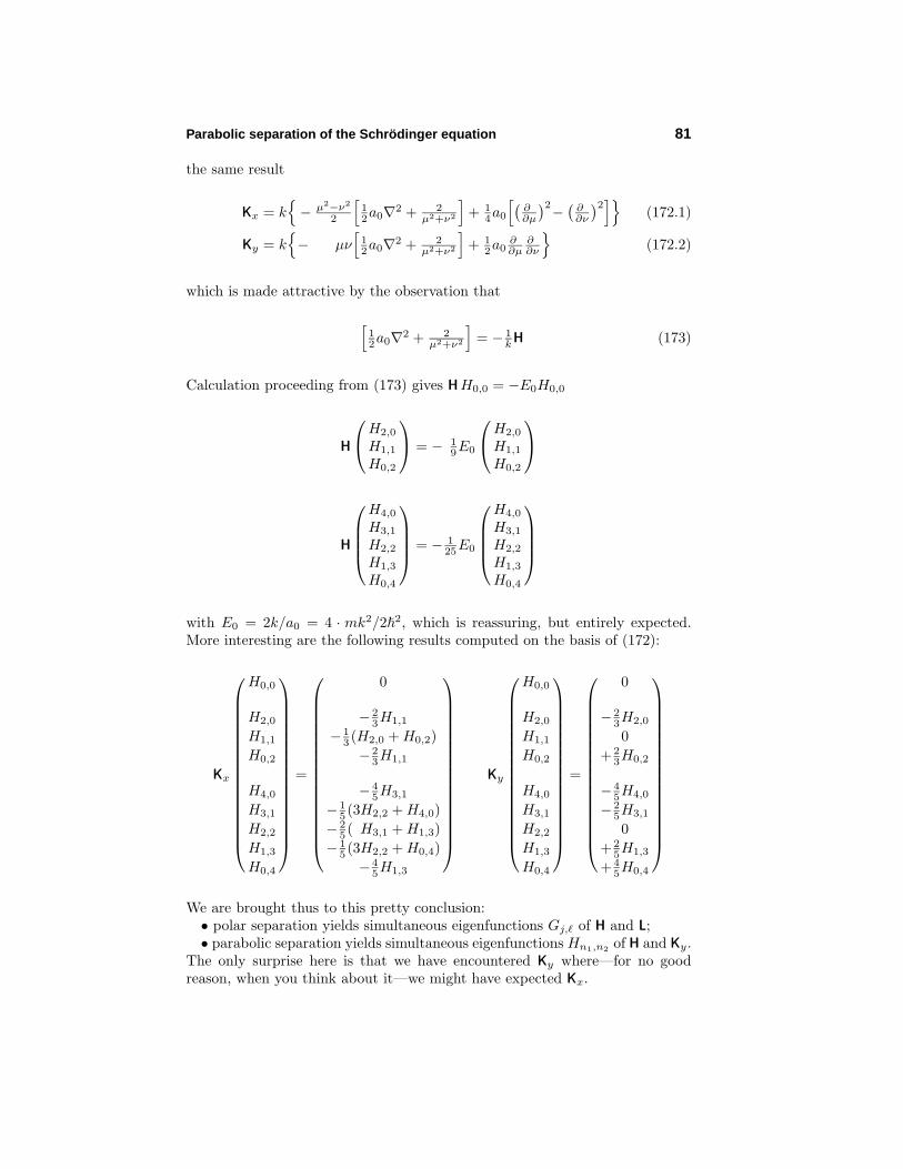
Parabolic separation of the Schrodinger equation 81
the same result
Kx = k− µ2−ν2
2
[12a0∇2 + 2
µ2+ν2
]+ 1
4a0
[(∂∂µ
)2−(∂∂ν
)2]
(172.1)
Ky = k− µν
[12a0∇2 + 2
µ2+ν2
]+ 1
2a0∂∂µ
∂∂ν
(172.2)
which is made attractive by the observation that
[12a0∇2 + 2
µ2+ν2
]= − 1
kH (173)
Calculation proceeding from (173) gives HH0,0 = −E0H0,0
H
H2,0
H1,1
H0,2
= − 1
9E0
H2,0
H1,1
H0,2
H
H4,0
H3,1
H2,2
H1,3
H0,4
= − 1
25E0
H4,0
H3,1
H2,2
H1,3
H0,4
with E0 = 2k/a0 = 4 · mk2/22, which is reassuring, but entirely expected.
More interesting are the following results computed on the basis of (172):
Kx
H0,0
H2,0
H1,1
H0,2
H4,0
H3,1
H2,2
H1,3
H0,4
=
0
− 23H1,1
− 13 (H2,0 + H0,2)− 2
3H1,1
− 45H3,1
− 15 (3H2,2 + H4,0)− 2
5 ( H3,1 + H1,3)− 1
5 (3H2,2 + H0,4)− 4
5H1,3
Ky
H0,0
H2,0
H1,1
H0,2
H4,0
H3,1
H2,2
H1,3
H0,4
=
0
− 23H2,0
0+ 2
3H0,2
− 45H4,0
− 25H3,1
0+ 2
5H1,3
+ 45H0,4
We are brought thus to this pretty conclusion:• polar separation yields simultaneous eigenfunctions Gj, of H and L;• parabolic separation yields simultaneous eigenfunctions Hn1,n2 of H and Ky.
The only surprise here is that we have encountered Ky where—for no goodreason, when you think about it—we might have expected Kx.
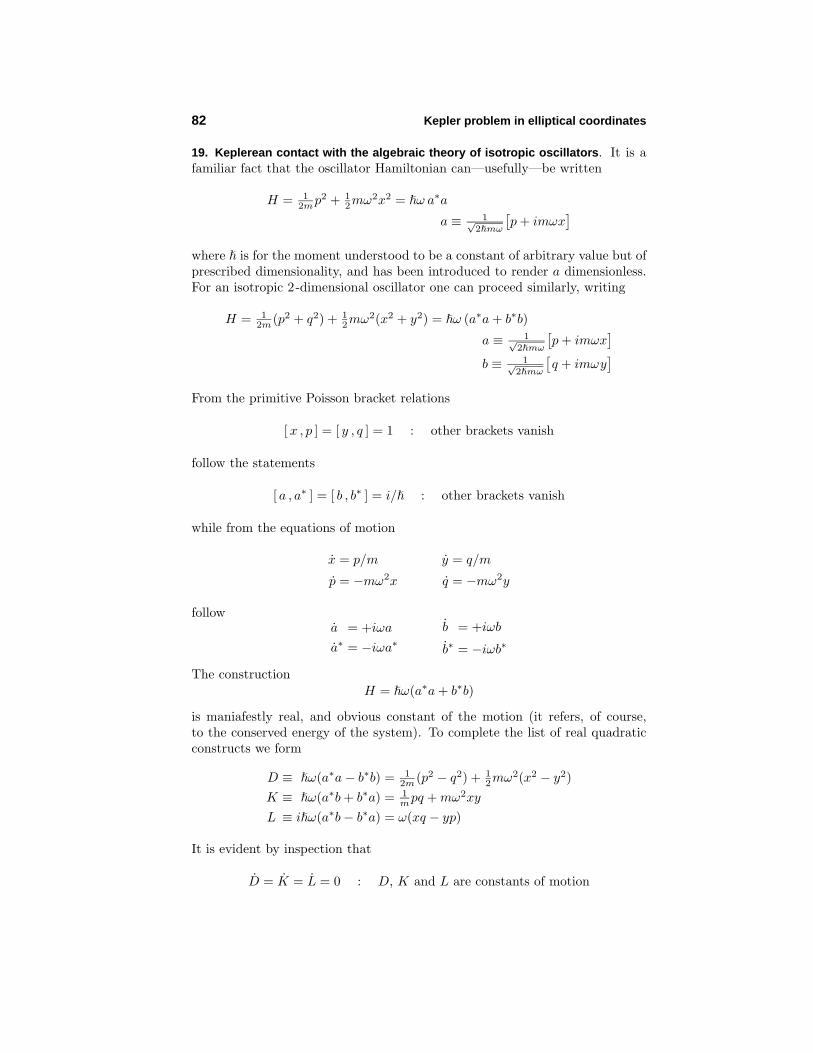
82 Kepler problem in elliptical coordinates
19. Keplerean contact with the algebraic theory of isotropic oscillators. It is afamiliar fact that the oscillator Hamiltonian can—usefully—be written
H = 12mp2 + 1
2mω2x2 = ω a∗a
a ≡ 1√2mω
[p + imωx
]where is for the moment understood to be a constant of arbitrary value but ofprescribed dimensionality, and has been introduced to render a dimensionless.For an isotropic 2-dimensional oscillator one can proceed similarly, writing
H = 12m (p2 + q2) + 1
2mω2(x2 + y2) = ω (a∗a + b∗b)
a ≡ 1√2mω
[p + imωx
]b ≡ 1√
2mω
[q + imωy
]From the primitive Poisson bracket relations
[x , p ] = [ y , q ] = 1 : other brackets vanish
follow the statements
[ a , a∗ ] = [ b , b∗ ] = i/ : other brackets vanish
while from the equations of motion
x = p/m
p = −mω2x
y = q/m
q = −mω2y
followa = +iωa
a∗ = −iωa∗b = +iωb
b∗ = −iωb∗
The constructionH = ω(a∗a + b∗b)
is maniafestly real, and obvious constant of the motion (it refers, of course,to the conserved energy of the system). To complete the list of real quadraticconstructs we form
D ≡ ω(a∗a− b∗b) = 12m (p2 − q2) + 1
2mω2(x2 − y2)K ≡ ω(a∗b + b∗a) = 1
mpq + mω2xy
L ≡ iω(a∗b− b∗a) = ω(xq − yp)
It is evident by inspection that
D = K = L = 0 : D, K and L are constants of motion
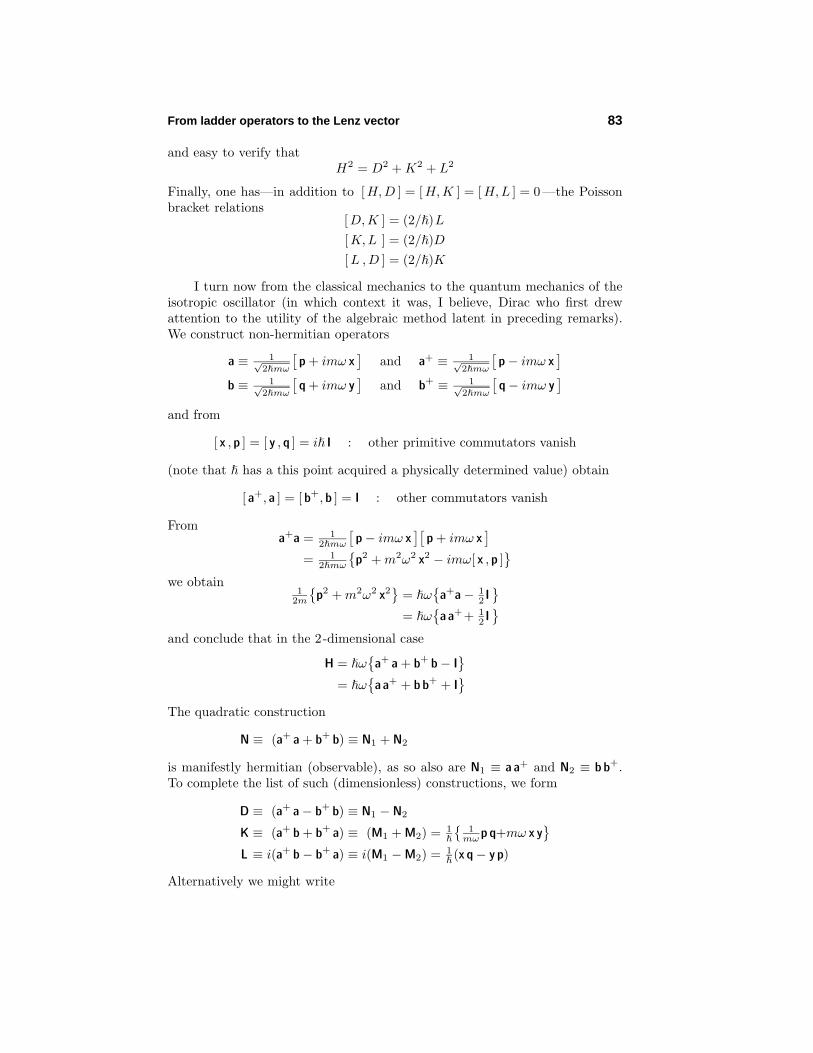
From ladder operators to the Lenz vector 83
and easy to verify thatH2 = D2 + K2 + L2
Finally, one has—in addition to [H,D ] = [H,K ] = [H,L ] = 0 —the Poissonbracket relations
[D,K ] = (2/)L[K,L ] = (2/)D[L ,D ] = (2/)K
I turn now from the classical mechanics to the quantum mechanics of theisotropic oscillator (in which context it was, I believe, Dirac who first drewattention to the utility of the algebraic method latent in preceding remarks).We construct non-hermitian operators
a ≡ 1√2mω
[p + imω x
]and a+ ≡ 1√
2mω
[p− imω x
]b ≡ 1√
2mω
[q + imω y
]and b+ ≡ 1√
2mω
[q− imω y
]and from
[ x , p ] = [ y , q ] = i I : other primitive commutators vanish
(note that has a this point acquired a physically determined value) obtain
[ a+, a ] = [ b+, b ] = I : other commutators vanish
Froma+a = 1
2mω
[p− imω x
][p + imω x
]= 1
2mω
p2 + m2ω2 x2 − imω[ x , p ]
we obtain
12m
p2 + m2ω2 x2
= ω
a+a− 1
2 I
= ωa a++ 1
2 I
and conclude that in the 2-dimensional case
H = ωa+ a + b+ b− I
= ω
a a+ + b b+ + I
The quadratic construction
N ≡ (a+ a + b+ b) ≡ N1 + N2
is manifestly hermitian (observable), as so also are N1 ≡ a a+ and N2 ≡ b b+.To complete the list of such (dimensionless) constructions, we form
D ≡ (a+ a− b+ b) ≡ N1 − N2
K ≡ (a+ b + b+ a) ≡ (M1 + M2) = 1
1
mωp q+mω x y
L ≡ i(a+ b− b+ a) ≡ i(M1 −M2) = 1(x q− y p)
Alternatively we might write

84 Kepler problem in elliptical coordinates
N =(
ab
)+(1 00 1
) (ab
)D =
(ab
)+(1 00 −1
) (ab
)
K =(
ab
)+(0 11 0
) (ab
)L =
(ab
)+(0 i−i 0
) (ab
)Computation65 gives
[ N ,D ] = [ N ,K ] = [ N , L ] = O
and[ D ,K ] = 2i L
[ K , L ] = 2iD
[ L ,D ] = 2iK
The latter equations mimic (to within an incidental sign) the commutationrelations satisfied by the traceless hermitian matrices
D ≡(
1 00 −1
)K ≡
(0 11 0
)L ≡
(0 i−i 0
)which we recognize to be “Pauli matrices”—generators of the fundamentalrepresentation of SU(2). Additional computation66 gives
D2 + K2 + L2 = N ( N− 222 )
The non-hermitian operators a , b and a+, b+ become up/down “ladderoperators”—and the hermitian operators N1 and N2 become at the same time“number opertors”—in consequence of the elementary facts summarized below:
N1 a = a ( N1 + I )N1 a+ = a+ ( N1 − I )N1 b = b N1
N1 b+ = b+ N1
N2 a = a N2
N2 a+ = a+ N2
N2 b = b (N2 + I )
N2 b+ = b+ ( N2 − I )
For if |ψ) is an eigenstate of N1 then so also is a|ψ), with eigenvalue incrementedby unity:
N1|ψ) = λ |ψ) =⇒
N1a |ψ) = (λ + 1) a |ψ)N1a
+|ψ) = (λ− 1) a+|ψ)etc.
65 It is simplest to proceed from the observation that
[ N1 ,N2 ] = O [ N1 ,M1 ] = −M1
[ N2 ,M1 ] = +M1
[ N1 ,M2 ] = +M2
[ N2 ,M2 ] = −M2
[ M1 ,M2 ] = N2 − N1
66 Easily D2+K2+L2 = N21−2N1N2+N2
2+2(2 M1M2+N1−N2). The argumentis completed by the observation that M1M2 = N1N2 − N1.
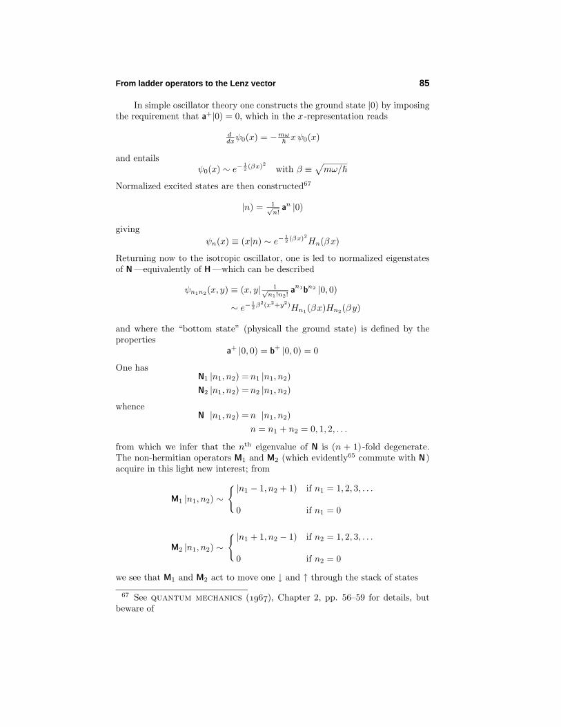
From ladder operators to the Lenz vector 85
In simple oscillator theory one constructs the ground state |0) by imposingthe requirement that a+|0) = 0, which in the x-representation reads
ddxψ0(x) = −mω
xψ0(x)
and entailsψ0(x) ∼ e−
12 (βx)2 with β ≡
√mω/
Normalized excited states are then constructed67
|n) = 1√n!
an |0)
givingψn(x) ≡ (x|n) ∼ e−
12 (βx)2Hn(βx)
Returning now to the isotropic oscillator, one is led to normalized eigenstatesof N —equivalently of H —which can be described
ψn1n2(x, y) ≡ (x, y| 1√n1!n2!
an1bn2 |0, 0)
∼ e−12β
2(x2+y2)Hn1(βx)Hn2(βy)
and where the “bottom state” (physicall the ground state) is defined by theproperties
a+ |0, 0) = b+ |0, 0) = 0
One hasN1 |n1, n2) =n1 |n1, n2)N2 |n1, n2) =n2 |n1, n2)
whenceN |n1, n2) =n |n1, n2)
n = n1 + n2 = 0, 1, 2, . . .
from which we infer that the nth eigenvalue of N is (n + 1)-fold degenerate.The non-hermitian operators M1 and M2 (which evidently65 commute with N)acquire in this light new interest; from
M1 |n1, n2) ∼ |n1 − 1, n2 + 1) if n1 = 1, 2, 3, . . .
0 if n1 = 0
M2 |n1, n2) ∼ |n1 + 1, n2 − 1) if n2 = 1, 2, 3, . . .
0 if n2 = 0
we see that M1 and M2 act to move one ↓ and ↑ through the stack of states
67 See quantum mechanics (), Chapter 2, pp. 56–59 for details, butbeware of

86 Kepler problem in elliptical coordinates
|n , 0)|n− 1, 1)|n− 2, 2)...|2, n− 2)|1, n− 1)|0, n )
which span the nth eigenspace of N, and within whichD,K , L
act to generate
an (n + 1)-dimensional representation of SU(2).
All of which has clear relevance to material that emerged from the parabolicformulation of the quantum mechanics of the 2-dimensional Kepler problem,though two fundamental distinctions have to be made:• The formal substitution
x, y
→
µ, ν
was found (p. 77) to entail that
we enforce the single-valuedness condition Ψ(µ, ν) = Ψ(−µ,−ν), and thusto require that in application to the Kepler problem we admit only evenvalues of n;• The formal substitution
β ≡√
mω
−→ α ≡√
2mk2(n+1)
brings into play an n-dependent scale factor which varies from eigenspaceto eigenspace.68 Bohr’s spectral formula (118/144) yields this alternativestatement
mω −→
The latter circumstance bedevils the design of the “Keplerean ladder operators,”in ways which Cisneros & McIntosh have labored to disentangle, but is relativelybenign as relates to operators (like N1, N2, M1 and M2, and operators assembledfrom them) which return eigenstates to the eigenspaces in which they originated.The force of the latter assertion is illustrated by the remarks which bring usnow to the point of this discussion:
In oscillator theory one has
N = N1 + N2 =
68 Note that the substitutions → involve replacing a variable/parameter byanother of different physical dimension.
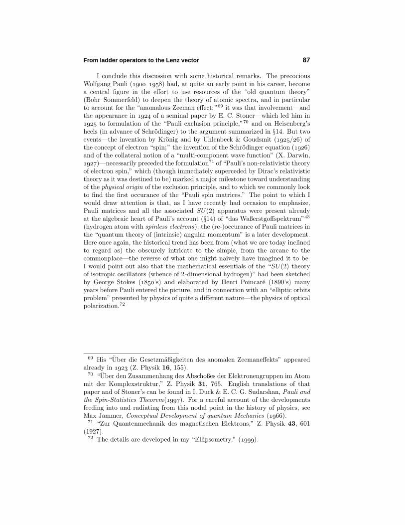
From ladder operators to the Lenz vector 87
I conclude this discussion with some historical remarks. The precociousWolfgang Pauli (–) had, at quite an early point in his career, becomea central figure in the effort to use resources of the “old quantum theory”(Bohr–Sommerfeld) to deepen the theory of atomic spectra, and in particularto account for the “anomalous Zeeman effect;”69 it was that involvement—andthe appearance in of a seminal paper by E. C. Stoner—which led him in to formulation of the “Pauli exclusion principle,”70 and on Heisenberg’sheels (in advance of Schrodinger) to the argument summarized in §14. But twoevents—the invention by Kronig and by Uhlenbeck & Goudsmit (/) ofthe concept of electron “spin;” the invention of the Schrodinger equation ()and of the collateral notion of a “multi-component wave function” (X. Darwin,)—necessarily preceded the formulation71 of “Pauli’s non-relativistic theoryof electron spin,” which (though immediately superceded by Dirac’s relativistictheory as it was destined to be) marked a major milestone toward understandingof the physical origin of the exclusion principle, and to which we commonly lookto find the first occurance of the “Pauli spin matrices.” The point to which Iwould draw attention is that, as I have recently had occasion to emphasize,Pauli matrices and all the associated SU(2) apparatus were present alreadyat the algebraic heart of Pauli’s account (§14) of “das Waßerstgoffspektrum”43
(hydrogen atom with spinless electrons); the (re-)occurance of Pauli matrices inthe “quantum theory of (intrinsic) angular momentum” is a later development.Here once again, the historical trend has been from (what we are today inclinedto regard as) the obscurely intricate to the simple, from the arcane to thecommonplace—the reverse of what one might naively have imagined it to be.I would point out also that the mathematical essentials of the “SU(2) theoryof isotropic oscillators (whence of 2-dimensional hydrogen)” had been sketchedby George Stokes (’s) and elaborated by Henri Poincare (1890’s) manyyears before Pauli entered the picture, and in connection with an “elliptic orbitsproblem” presented by physics of quite a different nature—the physics of opticalpolarization.72
69 His “Uber die Gesetzmaßigkeiten des anomalen Zeemaneffekts” appearedalready in (Z. Physik 16, 155).
70 “Uber den Zusammenhang des Abschoßes der Elektronengruppen im Atommit der Komplexstruktur,” Z. Physik 31, 765. English translations of thatpaper and of Stoner’s can be found in I. Duck & E. C. G. Sudarshan, Pauli andthe Spin-Statistics Theorem(). For a careful account of the developmentsfeeding into and radiating from this nodal point in the history of physics, seeMax Jammer, Conceptual Development of quantum Mechanics ().
71 “Zur Quantenmechanik des magnetischen Elektrons,” Z. Physik 43, 601(1927).
72 The details are developed in my “Ellipsometry,” ().