Embed Size (px)
Citation preview

i
REDUCED REFERENCE IMAGE QUALITY ASSESMENT
By
LAI MING JIE
A project report submitted in partial fulfilment of the requirements for the
award of Bachelor of Science (Hons.) Applied Mathematics with Computing
Faculty of Engineering and Science
Universiti Tunku Abdul Rahman
January 2016

ii
DECLARATION
I hereby declare that this project report entitled “REDUCED REFERENCE IMAGE
QUALITY ASSESSMENT” is my own work except for citations and quotations
which have been duly acknowledged. I also declare that it has not been previously and
concurrently submitted for any other degree or award at UTAR or other institutions.
Signature :
Name :
ID No. :
Date :

iii
APPROVAL FOR SUBMISSION
I certify that this project report entitled “REDUCED REFERENCE IMAGE
QUALITY ASSESSMENT” was prepared by LAI MING JIE has met the required
standard for submission in partial fulfilment of the requirements for the award of
Bachelor of Science (Hons.) Applied Mathematics With Computing at Universiti
Tunku Abdul Rahman.
Approved by,
Signature :
Supervisor :
Date :
iv
The copyright of this report belongs to the author under the terms of the
copyright Act1987 as qualified by Intellectual Property Policy of University Tunku
Abdul Rahman. Due acknowledgement shall always be made of the use of any material
contained in, or derived from, this report.
© 2016, LAI MING JIE. All rights reserved.

v
ACKNOWLEDGEMENTS
I would like to express my appreciation to my parents for their support in sending
me to Universiti Tunku Abdul Rahman to pursue the course I wanted, which is
Bachelor of Science (Hons.) Applied Mathematics with Computing. Other than
financially support, they always give me a lot of encouragement to handle the stress
that I faced during my university lives.
In addition, I want to thank my supervisor, Dr. Chang Yun Fah for guiding
me to complete this final year project, from the beginning until the end. Dr. Chang
always willing to share his thoughts and teach me a lot of extra knowledges which
guide me to think about my final year project. As a full-scheduled head of
department, lecturer, and many other final year students’ supervisor, Dr. Chang
always make his time to follow up with my progress. I am very thankful to have Dr.
Chang as my supervisor.
Furthermore, I want to thank my lecturers and my friends for their help.
Lecturers have taught me a lot of basic knowledges in mathematics and
programming. These basics have helped me in doing my final year project. Besides,
my friends do helped me a lot in completing my final year project. They always
willing to help me in using the build-in function of Microsoft Word to prepare my
final report. Moreover, when my laptop is broken down, they always offer me their
laptop to continue my work before my laptop recover.

vi
REDUCED REFERENCE IMAGE
QUALITY ASSESSMENT
ABSTRACT
Image quality assessment (IQA) is an analysis on the quality of an image. It is important
to ensure the quality of an image remains high after conversion through any software or
transmission from sender to receiver. This is because the image quality will affect the
applications of imaging technologies. There are three levels of image quality assessment
based on the availability on reference image, which are full reference (FR), no reference
(NR), and reduced reference (RR). This study aims to propose a new reduced reference
image quality metric (IQM), by way of statistical approach, for imperfect quality reference
image.
The new RR-IQM used the concept of logistic function, which demonstrates the
relationship between distortion level and image quality. The logistic model is used to
derive the image quality metric 𝑅𝐿2 =
𝑅𝑠2
𝐿 where the carrying capacity, L is estimated by
plotting graphs of sigma value, s which is the ratio of standard deviation for reference
image and distorted image and 𝑅𝑠2 is the coefficient of determination. The proposed 𝑅𝐿
2 is
a RR-IQM as the perfect reference image is unnecessary. In order to assess the
performance of 𝑅𝐿2, PLCC and MAE are used to test their monotonicity, whereas RMSE,
SRCC, and KRCC are used to assess its accuracy. A good IQM should have high PLCC,
SRCC, and KRCC values and low MAE and RMSE values.
The proposed 𝑅𝐿2 is then tested on a standard image database called LIVE. The
results show that 𝑅𝐿2 performs better than others IQMs if the reference image is degraded

vii
by JPEG2000 and it works reasonably well under JPEG and Gaussian Blur. In addition to
that, 𝑅𝐿2 has good monotonicity and accuracy when reference image is of greater quality.
For same distorted image, 𝑅𝐿2 provides more consistent results for over a range of
reference image qualities.

viii
TABLE OF CONTENTS
DECLARATION ii
APPROVAL FOR SUBMISSION iii
ACKNOWLEDGEMENTS v
ABSTRACT vi
TABLE OF CONTENTS viii
LIST OF TABLES xi
LIST OF FIGURE xiv
CHAPTER
1 INTRODUCTION 1
1-1 Motivation 2
1-2 Objectives 3
1-3 Scope of Study 4
1-4 Definition 5
2 LITERATURE REVIEW 6
2-1 Statistical prior models 6
2-2 Structural method 9

ix
2-3 Machine Learning 10
2-4 Metrics as comparison 11
...... 2-4-1 Structural Similarity (SSIM) Index 11
2-4-2 Peak signal-to-noise ratio (PSNR) 12
2-4-3 Estimate SSIM proposed by Z. Wang (2012) 13
2-4-4 Difference Mean Opinion Score (DMOS) 15
3 METHODOLOGY 16
3-1 Type of Distortion 16
3-2 Test Images 19
3-3 Proposed metric, 𝑅𝐿2 21
3-4 Estimate the carrying capacity, L 26
3-5 Measuring the performance of IQM 30
3-5-1 Pearson linear correlation coefficient (PLCC) 30
3-5-2 Mean absolute error (MAE) 31
3-5-3 Root mean-squared (RMS) error 32
3-5-4 Spearman’s rank correlation coefficient (SRCC) 32
3-5-5 Kendall’s rank correlation coefficient (KRCC) 33
3-6 Bit Rate of Distortions 33
4 RESULTS AND DISCUSSION 34
4-1 Performance of 𝑅𝐿2 When Reference Image Has Gaussian
Blur Distortion 35
4-1-1 JPEG distorted image as compressed image 35
4-1-2 JPEG2000 distorted image as compressed image 41

x
4-1-3 Gaussian Noise distorted image as compressed
image 47
4-1-4 Fast Fading distorted image as compressed image 53
4-2 Performance of 𝑅𝐿2 When Reference Image Has JPEG
Distortion 59
4-2-1 Gaussian Noise distorted image as compressed
image 59
4-2-2 Gaussian Blur distorted image as compressed
image 66
4-2-3 JPEG2000 distorted image as compressed
image 72
4-2-4 Fast Fading distorted image as compressed
image 78
4-3 Performance of 𝑅𝐿2 When Reference Image Has JPEG2000
Distortion 84
4-3-1 Gaussian Noise distorted image as compressed
image 85
4-3-2 Fast Fading distorted image as compressed
image 91
4-3-3 JPEG distorted image as compressed image 97
4-3-4 Gaussian Blur distorted image as compressed
image 103
5 CONCLUSION 110
REFERENCES 113

xi
LIST OF TABLES
TABLE TITLE PAGE
3-1 Information of the test images. 20
4-1 Results of each metrics applied on JPEG distorted image,
caps.bmp, with different level of bit rate. The reference
image used is with Gaussian blur distortion. 36
4-2 Results of each metrics used to judge the performance
of RR-IQA metrics used 38
4-3 Results of each metrics applied on a JPEG2000
compressed image, caps.bmp, with different level
of bit rate. The reference image used is with Gaussian
blur distortion. 42
4-4 Results of each metrics used to judge the performance
of RR-IQA metrics used. 45
4-5 Results of each metrics used to judge the performance
of RR-IQA metrics used. 48
4-6 Results of each metrics used to judge the performance
of RR-IQA metrics used. 51
4-7 Results of each metrics applied on a Fast Fading
compressed image, caps.bmp, with different level of
bit rate. The reference image used is with Gaussian blur
distortion. 54
4-8 Results of each metrics used to judge the performance
of RR-IQA metrics used. 57

xii
4-9 Results of each metrics applied on a Gaussian Noise
compressed image, caps.bmp, with different level of
bit rate. The reference image used is with JPEG distortion. 60
4-10 Results of each metrics used to judge the performance
of RR-IQA metrics used. 63
4-11 Results of each metrics applied on a Gaussian Blur
compressed image, caps.bmp, with different level of
bit rate. The reference image used is with JPEG distortion. 67
4-12 Results of each metrics used to judge the performance
of RR-IQA metrics used. 70
4-13 Results of each metrics applied on a JPEG2000
compressed image, caps.bmp, with different level of
bit rate. The reference image used is with JPEG distortion. 73
4-14 Results of each metrics used to judge the performance
of RR-IQA metrics used. 76
4-15 Results of each metrics applied on a fast fading
compressed image, caps.bmp, with different level of
bit rate. The reference image used is with JPEG distortion.. 79
4-16 Results of each metrics used to judge the performance
of RR-IQA metrics used. 81
4-17 Results of each metrics applied on a Gaussian Noise
compressed image, caps.bmp, with different level of
bit rate. The reference image used is with JPEG2000
distortion. 86
4-18 Results of each metrics used to judge the performance
of RR-IQA metrics used. 88
4-19 Results of each metrics applied on a Fast Fading
compressed image, caps.bmp, with different level of
bit rate. The reference image used is with JPEG2000
distortion. 92

xiii
4-20 Results of each metrics used to judge the performance
of RR-IQA metrics used. 95
4-21 Results of each metrics applied on a JPEG compressed
image, caps.bmp, with different level of bit rate. The
reference image used is with JPEG2000 distortion. 98
4-22 Results of each metrics used to judge the
performance of RR-IQA metrics used. 100
4-23 Results of each metrics applied on a Gaussian Blur
compressed image, caps.bmp, with different level of
bit rate. The reference image used is with JPEG2000
distortion. 104
4-24 Results of each metrics used to judge the performance
of RR-IQA metrics used. 107
5-1 Summary of the performance of each IQM. 111

xiv
LIST OF FIGURES
FIGURE TITLE PAGE
3-1 Samples of Gaussian blur distortion with bit rate
0 and 11.333325. 17
3-2 Samples of JPEG distortion with bit rate 0 and
2.7772. 17
3-3 Samples of JPEG2000 distortion with bit rate 0
and 2.9056. 18
3-4 Samples of fast fading distortion with bit rate 0 and 16.5. 18
3-5 Samples of Gaussian Noise distortion with bit rate 0 and 1.0. 19
3-6 Example of test images used, Caps.bmp 21
3-7 Logistic relationship between compression quality factor
and image quality. 22
3-8 Graph plotted by s versus 𝑅𝑠2, for Gaussian blur distortion. 27
3-9 Graph plotted by s versus 𝑅𝑠2, for JPEG distortion. 28
3-10 Graph plotted by s versus 𝑅𝑠2, for JPEG2000 distortion. 29
4-1 Graph plotted to show the relationship of each metrics,
with different bit rate value of JPEG distorted value,
and different level of distortion for Gaussian blur
distorted reference image. 40
4-2 Graph plotted to show the relationship of each metrics,
with different bit rate value of JPEG2000 distorted value,
and different level of distortion for Gaussian blur
distorted reference image. 46

xv
4-3 Graph plotted to show the relationship of each metrics,
with different bit rate value of Gaussian Noise distorted
value, and different level of distortion for Gaussian blur
distorted reference image. 52
4-4 Graph plotted to show the relationship of each metrics,
with different bit rate value of fast fading distorted value,
and different level of distortion for Gaussian blur distorted
reference image. 58
4-5 Graph plotted to show the relationship of each metrics,
with different bit rate value of Gaussian Noise distorted
value, and different level of distortion for JPEG distorted
reference image. 65
4-6 Graph plotted to show the relationship of each metrics,
with different bit rate value of fast fading distorted value,
and different level of distortion for Gaussian blur distorted
reference image. 71
4-7 Graph plotted to show the relationship of each metrics,
with different bit rate value of fast fading distorted value,
and different level of distortion for JPEG distorted r
eference image. 77
4-8 Graph plotted to show the relationship of each metrics,
with different bit rate value of fast fading distorted value,
and different level of distortion for JPEG distorted
reference image. 83
4-9 Graph plotted to show the relationship of each metrics,
with different bit rate value of Gaussian Noise distorted
value, and different level of distortion for JPEG2000
distorted reference image. 90
4-10 Graph plotted to show the relationship of each metrics,
with different bit rate value of fast fading distorted value,
xvi
and different level of distortion for JPEG2000 distorted
reference image. 96
4-11 Graph plotted to show the relationship of each metrics,
with different bit rate value of JPEG distorted value,
and different level of distortion for JPEG2000 distorted
reference image. 102
4-12 Graph plotted to show the relationship of each metrics,
with different bit rate value of Gaussian Blur distorted
value, and different level of distortion for JPEG2000
distorted reference image. 108

1
CHAPTER 1
INTRODUCTION
Digital images are economical and efficient medium for communicating information. It
has greatly influenced the modern lifestyle, for example telemedicine, satellite imaging,
biometric surveillance, advertisement and entertainment. The quality of an image will
affect the applications of imaging technologies. In such, more and more experts proposed
and improved different methods of image quality assessment metric (IQM), to enrich the
image processing application. IQM provides an objective indicator of the perceived
quality of an image. Generally, IQM has three types of application, which are to keep
tracking the quality of images for quality control systems, to standardized image
processing algorithms, and to enhance the parameter settings.
An image is distorted after it is converted through any software or transmitting
from sender to receiver. It has to pass through several stages before it reach the receiver.
Those distortions or noises are generated and added into the image at those stages of image
processing, such as image acquisition, image compression, and image reconstruction. In
order to make sure that the receiver get the same quality of image as the sender, IQM acts
an important role in it. According to an articles, the reporters say that the best way to assess
the quality of an image is perhaps to look at it because human eyes are the ultimate
receivers in most image processing environments. However, this is a very subjective
opinion from different people, moreover with different visionary ability. Therefore, IQA
measurements is developed to assess different images provided by different fields of users.

2
Mainly, the IQM algorithms can be divided into three levels, which are full
reference (FR), reduced reference (RR), and no reference (NR). Full reference (FR) IQA
is that an image, which is free of distortion and considered perfect in quality, is used as
the reference image. Reduced reference (RR) IQA is, by using an imperfect quality image
as the reference image. On the other hand, no reference image is given for no reference
(NR) IQA, to carry out the assessment. Most of the IQM proposed is FR-IQM, as it is
considered as the easiest way to construct the metric. However, this study is look into RR-
IQM, and a new RR-IQM is proposed.
1-1 Motivation
Image quality is an important topic as it will affect the output analysis of certain aspects,
especially for medical imaging. The medical imaging continues to play a stronger role in
diagnosis of diseases and treatment, the importance of image quality relatively rises. A
pleasing or beautiful image alone does not indicate an accurate diagnosis. Therefore, a
necessity of the efforts of the image quality assessment and medical imaging professionals
is required to optimize the quality and safety of health care to ensure the optimal outcome.
The similar theory is applied to the satellite image. The photo grain that always appear in
space photos may limit the information contents of digitized photo. A good image quality
will definitely improve this limitation and give a hand in the development of topography.
On the other hand, by improving image quality will indirectly improve the quality
of lives. Most of the entertainment today involve visual enjoyment, such as videos, movies,
animations and photos. An obvious example is from the Korean Pop (K-pop) industry.
The major selling point of K-pop is about music, which is about listening. However,
another important aspect is the visual genre. Even the successful of a song or artist began
to rely on television during the 1980s. Most of the music programs started to dedicate in
live performances, talk shows, musical dramas, different types of show, behind-the-scenes

3
documentaries, and music videos (MV). This has shown a great improving of quality of
lives as people are upgraded from listening enjoyment to visual and audio enjoyment.
Furthermore, image quality does act an important role in business industry. People
rely on imaginary to share information, learn about new knowledge, and get themselves
involved on things that they are interested. Using images in business works in a same way,
which help people to feel and see the products and services without relying on written
messages only. A high quality images, and illustrations will definitely increase the interest
and excitement of the customers. Besides, a good quality of video during video
conferencing will enhance the progress of a meeting. Business partner from different
places manage to call out a meeting together, just like face to face meeting if the video
conferencing have a good quality. This will save time and cost of travelling, and to make
sure that an important business issue is not delayed.
1-2 Objectives
In this study, a new IQM is proposed to provide an objective indicator of the perceived
quality of an image. This study has the following objectives
1. To survey different image quality assessment metrics (IQM) from various
articles and journals. The methods, advantages and disadvantages of those
metrics is studied.
2. To develop a new reduced reference image quality measurement using logistic
concept.
3. To evaluate the performance the proposed IQM in various distortion types of
reference image.

4
4. To apply the proposed metric to certain distortion type of imperfect reference
images, which are Gaussian blur, JPEG and JPEG2000 distortion. This is to
ensure that the metric proposed is suitable for the targeted images.
1-3 Scope of Study
In IQA field, there are three levels of assessment available, which are full reference (FR), reduced
reference (RR), and no reference (NR). In this study, only reduced reference IQA is considered. This
is because RR-IQA has plenty of metrics proposed in this filed, we need to propose a more
practically useful IQM to help in improving this field. We use a statistical way to construct the RR-
IQM in this study.
There are quite a number of image database provided, such as Cornell-A57 database, IVC
database, Toyama-MICT database, Tampere Image database, and more. By using images from
different database can provide a more accurate result for IQA, as different characteristics can be
found from different database. However in this study, only images in LIVE database is used in this
study due to time constrain. LIVE database contains 982 images in total, where 779 of them are
distorted with five different types of distortion.
In this study, only three types of distortion is included for imperfect reference image, which
are Gaussian Blur, JPEG, and JEPG2000. When estimating the carrying capacity, L for each
distortion types, more accurate result is found for these three distortion types. Gaussian Noise and
Fast Fading distortion type do not get the accurate carrying capacity value. This may due to fewer
images is included in predicting the carrying capacity value.

5
1-4 Definition
IQA can be divided into three levels, which are full reference (FR), reduced reference
(RR), and no reference (NR). Full reference (FR) IQA is that, a reference image, which is
free of distortion and considered as perfect in quality, is given. Then, a distorted image is
given as well to make an assessment between them. FR-IQA is considered as the easiest
way to assess an image quality, as a perfect quality of reference image is used. However,
it is sometimes impractical in actual as it is difficult to obtain an original perfect quality
image as the full reference.
In reduced reference (RR) IQA problem, an imperfect quality image is provided
as the reference image, to carry out assessment with the distorted image given. Basically,
there are three types of RR-IQA. The first one is that only some variables of reference
image is available to carry out the IQA. Secondly, only certain part of the reference image
is given. Lastly, only a corrupted reference image and standard deviations of both
reference image and distorted image are given, where this is the type of RR-IQA studied
in this study. RR-IQA is more practically used, as a reference image we can get in actual
lives is mostly without perfect quality. When an RR-IQA is used, only certain information
are needed based on the IQM algorithm’s structure.
For no reference (NR) IQA, no reference image is given, but only the distorted
image. An algorithm need to be developed to assess the quality of image provided itself
without doing any referencing. NR-IQA can be considered as an ideal IQA but is the most
difficult one. Up to date, there is still lack of successful NR-IQM algorithm in the field.

6
CHAPTER 2
LITERATURE REVIEW
Over the decade, the reduced reference (RR) image quality assessment (IQA) is mostly
studied among all. Structural similarity (SSIM) index is seldom been used, as it is more
suitable for full reference (FR) metric. Majority of the reduce reference IQA performed
were related to logarithm function. There are three categories of metrics will be reviewed.
2-1 Statistical prior models
Statistical regression method is being used in developing image quality assessment
method. Xue&Mou (2010) have proposed a new method named βW-SCM to estimate the
quality of distorted image. It requires two steps before performing the new method, which
are defining the SCM for redundancy reduction to present image features, and employing
Weibull distribution to describe the statistics of SCM and scale parameter β is extracted
as reduced reference feature. (Xue&Mou 2010)The final perceptual distortion of the tested
image proposed is defined as

7
𝐷𝛽𝑊−𝑆𝐶𝑀 = ∑√𝑑𝐴𝑛 × 𝑑𝑅
𝑛
6
𝑛=1
where 𝑑𝐴𝑛 is the absolute deviation, 𝑑𝑅
𝑛 is the relative deviation, and N is the total number
of scales. (Xue&Mou2010) This new method uses less reduced reference feature and has
a short execution time. However, it needs to perform two steps before execute the new
method proposed, which may consider lengthy steps and time consumed.
Zhang et al (2011) proposed a simple edge verification method for RR-IQA metric.
Only 12 scalar features are needed as compared to other RR IQA model which need 16
scalar features. (Zhang et al 2011)The predicted objective score for one image is defined
as
𝐷𝑀 =∑∑𝑙𝑜𝑔10[𝑝𝑐𝑖(𝑥𝑘) − 𝑝𝐷𝑖(𝑥𝑘)]2
3
𝑘=1
4
𝑖=1
where 𝑝𝑐𝑖(𝑥𝑘) and 𝑝𝐷𝑖(𝑥𝑘) is the normalized histogram comes from the statistics of the
edge pattern maps 𝐶𝑖𝑝
and 𝐷𝑖𝑝. (Zhang et al 2011)The proposed algorithm is simple, but
the data rate is lower than other well-known IQA. (Zhang et al 2011)
D. Yang et al (2012) focus their research of RR-IQA metric based on natural image
statistic in Roberts cross derivative domain. Roberts cross derivative (L.S. Davis 1975) is
widely used in detecting image edges which are important geometric feature about image
for visual prediction. (D. Yang et al 2012) The overall distortion between the reference
and distorted image is defined as
𝐷𝑖𝑠𝑡𝑜𝑟𝑡𝑖𝑜𝑛 = 𝑙𝑜𝑔2(1 +𝐷𝑅𝐴𝐷𝑋 (𝑝𝑋, 𝑞𝑋)𝐷𝜎2
𝑋 𝐷𝑘𝑋𝐷𝑆
𝑋 +𝐷𝑅𝐴𝐷𝑌 (𝑝𝑌 , 𝑞𝑌)𝐷𝜎2
𝑌 𝐷𝑘𝑌𝐷𝑆
𝑌
2𝐷0)

8
where X and Y are associated the main diagonal and the anti-diagonal of image,
respectively, 𝑝𝑋 and 𝑞𝑋 (𝑝𝑌 and 𝑞𝑌) denote the probability density functions of Roberts
cross derivative in the reference and distorted images, respectively,
𝐷𝐾𝐿𝐷𝑌 (𝑝𝑌 , 𝑞𝑌) (𝐷𝐾𝐿𝐷
𝑋 (𝑝𝑋, 𝑞𝑋)) is the estimation of KLD between 𝑝𝑋 and 𝑞𝑋 (𝑝𝑌 and 𝑞𝑌),
and 𝐷𝜎2𝑋 (𝐷𝜎2
𝑌 ), 𝐷𝑘𝑋(𝐷𝑘
𝑌), 𝐷𝑆𝑋 (𝐷𝑆
𝑌) are the comparisons of variance, kurtosis and skewness,
respectively. (D. Yang et al 2012) The proposed metric is less complex as compared to
other RR-IQA, as only twelve parameters from the reference image is needed.(D. Yang et
al 2012)Moreover, the metric can be applied for all distortion types and has a good
performance as compared to other popular RR-IQA. (D. Yang et al 2012)
The coefficient of determination derived from MULFR (Multidimensional
replicate linear functional relationship) model proposed by Y. F. Chang et al (2008), is
used for correlation measure, denoted by 𝑅𝐹2. The specialty of this measurement is where
it assumes both the reference and compressed images is subjected to errors, and uses
several quality attributes to calculate overall image similarity value. (Y.F. Chang et al
2008) Numerous quality attributes computed from local windows are used to calculate the
overall image similarity value.
The similarity measure,𝑅𝐹2is defined as
𝑅𝑓2 =
𝑆𝑆𝑅𝑆𝑦𝑦
= ��𝑆𝑥𝑦𝑆𝑦𝑦
where �� = (𝑆𝑦𝑦−𝜆𝑆𝑥𝑥)+ √(𝑆𝑦𝑦−𝜆𝑆𝑥𝑥)
2+4𝜆𝑆𝑥𝑦2
2𝑆𝑥𝑦, �� = (��1, ��2, … , ��𝑝)′ , �� = (��1, ��2, … , ��𝑝)′ ,
𝑆𝑥𝑥 = ∑ 𝑥𝑖′𝑥𝑖 − 𝑛𝑥
′𝑥 𝑛𝑖=1 , 𝑆𝑦𝑦 = ∑ 𝑦𝑖
′𝑦𝑖 − 𝑛𝑦′𝑦𝑛
𝑖=1 and 𝑆𝑥𝑦 = ∑ 𝑥𝑖′𝑦𝑖
𝑛𝑖=1 − 𝑛𝑥 ′𝑦.
The value of 𝑅𝐹2 shows the proportion of variation in reference image explained by the
distorted image.
9
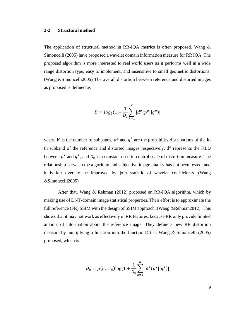
2-2 Structural method
The application of structural method in RR-IQA metrics is often proposed. Wang &
Simoncelli (2005) have proposed a wavelet domain information measure for RR IQA. The
proposed algorithm is more interested to real world users as it performs well in a wide
range distortion type, easy to implement, and insensitive to small geometric distortions.
(Wang &Simoncelli2005) The overall distortion between reference and distorted images
as proposed is defined as
𝐷 = 𝑙𝑜𝑔2 (1 +1
𝐷0∑|𝑑𝑘(𝑝𝑘||𝑞𝑘)|
𝐾
𝑘=1
where K is the number of subbands, 𝑝𝑘 and 𝑞𝑘 are the probability distributions of the k-
th subband of the reference and distorted images respectively, 𝑑𝑘 represents the KLD
between 𝑝𝑘 and 𝑞𝑘, and 𝐷0 is a constant used to control scale of distortion measure. The
relationship between the algorithm and subjective image quality has not been tested, and
it is left over to be improved by join statistic of wavelet coefficients. (Wang
&Simoncelli2005)
After that, Wang & Rehman (2012) proposed an RR-IQA algorithm, which by
making use of DNT-domain image statistical properties. Their effort is to approximate the
full reference (FR) SSIM with the design of SSIM approach. (Wang &Rehman2012) This
shows that it may not work as effectively in RR features, because RR only provide limited
amount of information about the reference image. They define a new RR distortion
measure by multiplying a function into the function D that Wang & Simoncelli (2005)
proposed, which is
𝐷𝑛 = 𝑔(𝜎𝑟 , 𝜎𝑑)log (1 +1
𝐷0∑|𝑑𝑘(𝑝𝑘||𝑞𝑘)|
𝐾
𝑘=1

10
The estimated SSIM value is used as a benchmark for my study. Their method will be
further discuss in the methodology part.
J. Wu et al (n.d.) introduced a RR-IQA metric which use less reference data and
achieve higher prediction accuracy. They suggested to represent the image structure by
using the local binary pattern (LBP), which is a popular and well accepted structural
descriptor, to extract structural information. (J. Wu et al n.d.)The main structural
degradation proposed is defined as
𝐻𝐶(𝐼𝑖𝑑, 𝐼𝑖
𝑜) =2 × 𝐻𝑖
𝑑 ∙ 𝐻𝑖𝑜
(𝐻𝑖𝑑)2 + (𝐻𝑖
𝑜)2
where 𝑖 ∈ {𝑝, 𝑟}. The RR-IQA proposed is generally a good RR-IQA as it meet a high
consistent. (J. Wu et al n.d.) However, it takes a lengthy steps to get the final result that
need to perform several procedures.
2-3 Machine Learning
Machine learning method is introduced in the development of RR IQA. This method is
considered a new method which a recent article is found studied about it. Mocanu et al
(2015) introduced a novel stochastic RR-IQA metric, called RBMSim. It evaluates on two
subjective benchmarked image databases. (Mocanu et al 2015)The RBMSim metric is
defined as

11
𝑅𝐵𝑀𝑆𝑖𝑚(𝐷𝐼) = √1
𝑛𝑣∑(𝑣𝑖
𝐷𝐼 − 𝑣𝑖𝐷𝐼)2
𝑛𝑣
𝑖=1
where 𝑛𝑣 is the number of visible neurons.RBMSim has a fast computational time and is
therefore suitable for online applications. (Mocanu et al 2015)The author left a further
discussion on to adapt RBMSim to videos by training RBMSim on all frames of video.
2-4 Metrics as comparison
Among the IQA proposed and exist for statistical prior model, SSIM, PSNR, estimated
RR-SSIM, and DMOS are used as major comparison with the method proposed, 𝑅𝐿2. SSIM
and PSNR are used, as SSIM is a popular FR-IQA, whereas PSNR is a traditional method,
which is commonly used. The estimated RR-SSIM, proposed by Z. Wang (2012) is the
latest RR-IQA proposed, which has a better accuracy, consistency, and monotonicity.
DMOS (Difference Mean Opinion Score) is a metric used for decades to obtain the
human’s user view of the quality of an image. Therefore, these four metrics are used as a
comparison in this study.
2-4-1 Structural Similarity (SSIM) Index
Structural similarity (SSIM) index is a method to measure the similarity between two
images. SSIM is a full reference image quality assessment metric. It is designed and

12
proposed to improve the older metrics, such as peak signal-to-noise ratio (PSNR) and
mean square error (MSE) metrics.
SSIM between two images x and y of common size is defined as
𝑆𝑆𝐼𝑀(𝑥, 𝑦) = (2𝜇𝑥𝜇𝑦 + 𝑐1)(2𝜎𝑥𝑦 + 𝑐2)
(𝜇𝑥2 + 𝜇𝑦2 + 𝑐1)(𝜎𝑥2 + 𝜎𝑦2 + 𝑐2)
where 𝜇𝑥 is the average of x, 𝜇𝑦 is the average of y, 𝜎𝑥2 is the variance of x, 𝜎𝑦
2 is the
variance of y, 𝜎𝑥𝑦 is the covariance of x and y, 𝑐1 = (𝑘1𝐿)2 and 𝑐2 = (𝑘2𝐿)
2 are two
variables to stabilize the division with weak denominator, with L is the dynamic range of
the pixel-values, and 𝑘1 = 0.01, 𝑘2 = 0.03 by default.
2-4-2 Peak signal-to-noise ratio (PSNR)
The peak signal-to-noise ratio (PSNR) is the ratio between the maximum possible power
of a signal and the power of distorted noise that affects its representation. PSNR is usually
expressed in terms of logarithmic scale. Normally, a higher PSNR value means that image
is of higher quality.
PSNR is more easily to define through the mean squared error (MSE), which is
defined as
𝑀𝑆𝐸 = 1
𝑚𝑛∑∑[𝐼(𝑖, 𝑗) − 𝐾(𝑖, 𝑗)]2
𝑛−1
𝑗=0
𝑚−1
𝑖=0

13
where 𝑚 × 𝑛 is the size of a grayscale image 𝐼, 𝐾 is the noise approximation.
The PSNR is defined as
𝑃𝑆𝑁𝑅 = 20 𝑙𝑜𝑔10(𝑀𝐴𝑋𝐼) − 10 𝑙𝑜𝑔10(𝑀𝑆𝐸)
where 𝑀𝐴𝑋𝐼 is the maximum pixel value of the image.
2-4-3 Estimate SSIM proposed by Z. Wang (2012)
The SSIM proposed by Z. Wang (2012) is estimated by using a straight-line relationship
between a newly defined reduced reference distortion measure,𝐷𝑛 and SSIM value. The
distortion of the distorted image is evaluated by the Kullback-Leibler divergence (KLD)
between the probability distribution of the original image, p(x) and the distorted image,
q(x). KLD is defined as
𝑑(𝑝||𝑞) = ∫𝑝𝑚(𝑥)𝑙𝑜𝑔𝑝(𝑥)
𝑞(𝑥)𝑑𝑥
where 𝑝𝑚(𝑥) is the model Gaussian distribution.
The new reduced reference distortion measure of the whole image is defined as
𝐷𝑛 = 𝑔(𝜎𝑟 , 𝜎𝑑)log (1 +1
𝐷0∑|𝑑
𝑘(𝑝𝑘||𝑞𝑘)|
𝐾
𝑘=1

14
where𝑝𝑘 and 𝑞𝑘 are the probability distributions of the k-th subband of the reference and
distorted images respectively, 𝑑𝑘 represents the KLD between 𝑝𝑘 and 𝑞𝑘 , and 𝑔(𝜎𝑟 , 𝜎𝑑)
is defined as
𝑔(𝜎𝑟 , 𝜎𝑑) = ||𝜎𝑟||
2 + ||𝜎𝑑||2 + 𝐶
2(𝜎𝑟 ∙ 𝜎𝑑) + 𝐶
where 𝜎𝑟 and 𝜎𝑑 represent the vectors containing standard deviation 𝜎 values, K is the
total number of subbands, C is a positive constant which is included to avoid instability
when the dot product𝜎𝑟 ∙ 𝜎𝑑 is close to 0.
For each fixed distortion type, 𝐷𝑛 exhibits a nearly perfect linear relationship with
SSIM. This relationship reduce the SSIM estimation problem to estimate the slope factor.
The straight-line relationship to estimate SSIM is defined as
�� = 1 − 𝛼𝐷𝑛
where 𝛼 is the slope factor.

15
2-4-4 Difference Mean Opinion Score (DMOS)
DMOS is the most straight forward way to determine the image quality. This is conducted
by asking a group of people to rate an image sequence relative to a full reference image.
The range of the DMOS value is rated differently for each researcher. In this study, the
range is as follow
0 - 20 – Very Satisfied
21 - 40 – Satisfied
41 - 60 – Some Users Satisfied
61 - 80 – Many Users Dissatisfied
81 - 100 – Most Users Dissatisfied
16
CHAPTER 3
METHODOLOGY
From the discussion in Chapter 2 literature review, we have seen the needs for proposing
a new RR-IQA for statistical approach. The proposed metric 𝑅𝐿2 is majorly based on the
MULFR model, 𝑅𝐹2 proposed by Chang Y. F. (2008). On the proposing of this metric,
various types of distortions are included in the study as the imperfect reference image and
distorted image. Those images are taken from LIVE database, which is widely used by the
researchers when proposing an IQA metric. Besides, it is important to know the
performance of a metric proposed to assess the quality of images. In this study, the
performance of the metric proposed is examined by five evaluation methods.
3-1 Type of Distortion
There are five distortion types involved in this study, which are Gaussian blur, JPEG,
JPEG2000, Fast Fading, and Gaussian Noise. Gaussian Blur, JPEG, and JPEG2000
distortions, with different bit rate are used as the imperfect reference image. For each of

17
the different imperfect reference image, another four types of distortions are used in the
distorted image to carry out this study.
Figure 3-1: Samples of Gaussian Blur Distortion with Bit Rate 0 and 11.333325.
Gaussian blur is a distortion type which having the result of blurring an image. It
is typically used in reduce the image noise or to reduce the image details. In mathematics,
Gaussian blur is performed by combining an image with Gaussian function.
Figure 3-2: Samples of JPEG Distortion with Bit Rate 0 and 2.7772.
18
JPEG is a commonly used compression designed to compress images effectively.
The degree of compression can be adjusted that is the image quality factor. JPEG is the
acronym for Joint Photographic Experts Group, the name for the committee who created
JPEG. JPEG is generally uses a form of compression based on the discrete cosine
transform (DCT).
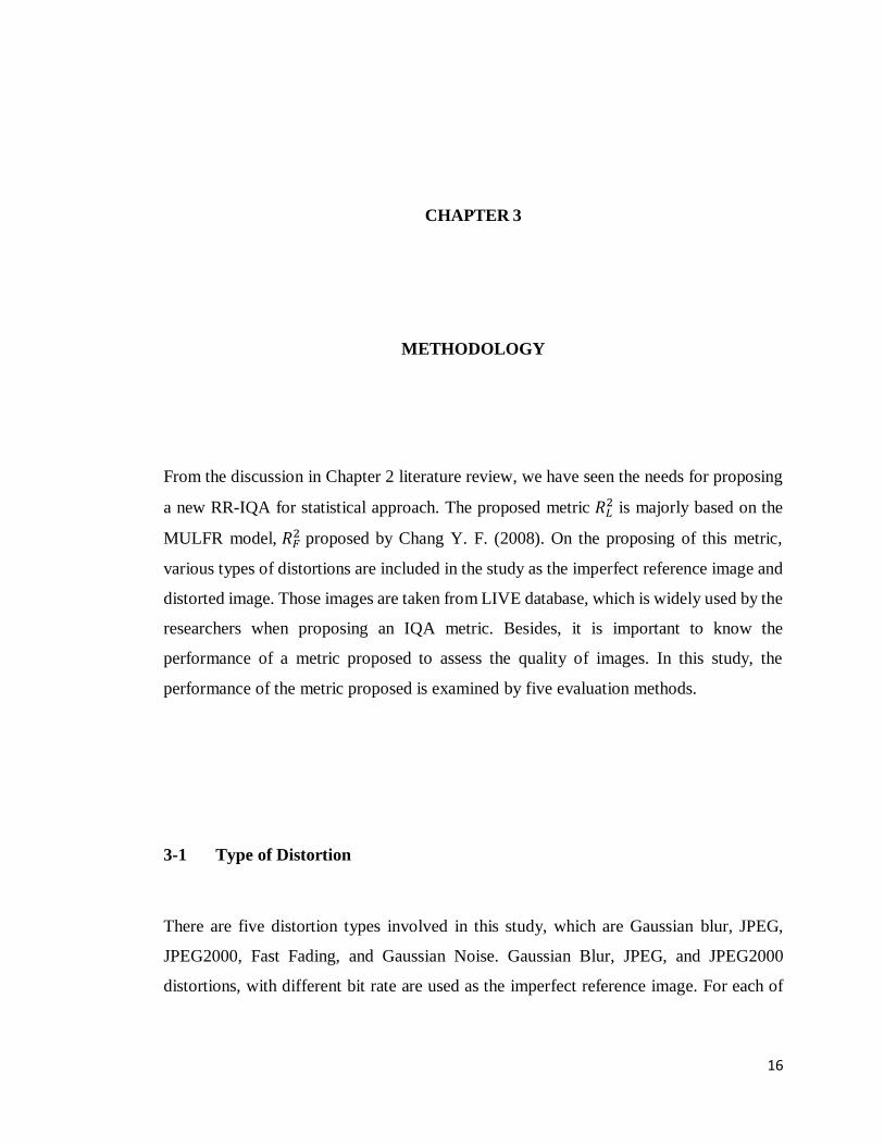
Figure 3-3: Samples of JPEG2000 Distortion with Bit Rate 0 and 2.9056.
JPEG2000 is a better image distortion or solution than JPEG. This is because it
compresses images with a lesser loss of visual performance. JPEG2000 is designed in year
2000, with a wavelet-based method. However, JPEG2000 is seldom being used due to its
complexity.
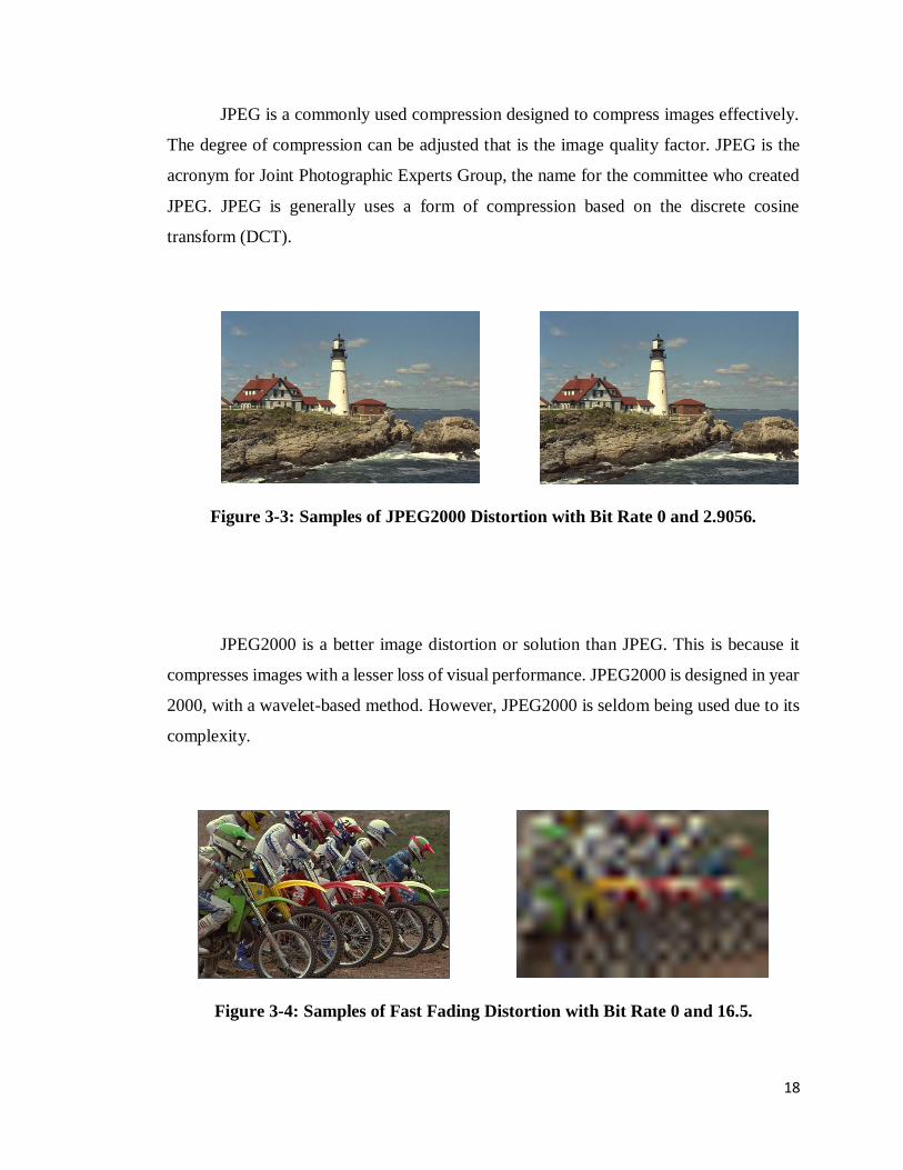
Figure 3-4: Samples of Fast Fading Distortion with Bit Rate 0 and 16.5.

19
Fading is the digression of a depletion affecting a media, such as images. It may
changes with time or radio frequency. Fast fading is where the frequency response changes
occur speedily. Practically, this type of distortion only occurs for very low data rates
images.
Figure 3-5: Samples of Gaussian Noise Distortion with Bit Rate 0 and 1.0.
Noise is the departure from the ideal image and the distorted image. Gaussian noise
often occur in acquisition process while sending an image. It can be caused by several
reasons, such as poor illumination, high temperature, and transmission.
3-2 Test Images
In this study, three types of distortion, which are Gaussian blur, JPEG, and JPEG2000
distortion with different bit rate each, are used in the imperfect reference image. On the
other hand, five types of distortion, which include Gaussian noise, fast fading, and the
three types of distortion mentioned previously, with different level of bit rate each, are

20
used as the distorted images. All of the images are from the LIVE database, which is a
database that is frequently used by most of the researchers in the literature review.
Table 3-1: Information of the Test Images.
Type of
Distortion
Number of
Images
Number of
Distortion
Gaussian Blur 29 67 × 29 = 1943
Gaussian Noise 29 56 × 29 = 1624
JPEG 29 159 × 29 = 4611
JPEG2000 29 149 × 29 = 4321
Fast Fading 29 11 × 29 = 319
21
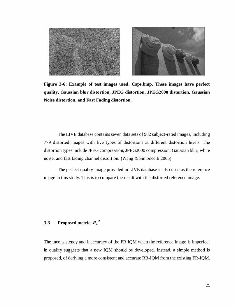
Figure 3-6: Example of test images used, Caps.bmp. These images have perfect
quality, Gaussian blur distortion, JPEG distortion, JPEG2000 distortion, Gaussian
Noise distortion, and Fast Fading distortion.
The LIVE database contains seven data sets of 982 subject-rated images, including
779 distorted images with five types of distortions at different distortion levels. The
distortion types include JPEG compression, JPEG2000 compression, Gaussian blur, white
noise, and fast fading channel distortion. (Wang & Simoncelli 2005)
The perfect quality image provided in LIVE database is also used as the reference
image in this study. This is to compare the result with the distorted reference image.
3-3 Proposed metric, 𝑹𝑳𝟐
The inconsistency and inaccuracy of the FR IQM when the reference image is imperfect
in quality suggests that a new IQM should be developed. Instead, a simple method is
proposed, of deriving a more consistent and accurate RR-IQM from the existing FR-IQM.

22
Logistic regression models the relationship between a dependent and one or more
independent variables. This allows us to look at the fitness of the model and the meaning
of the relationships that are modelling. In many ways, it is seems to be alike with ordinary
regression. However, there is a slight difference with ordinary linear regression. The
ordinary regression find the best fitting line by using ordinary least squares method, while
logistic regression calculate the probability of an event occur.
Image quality, 𝑅𝑠2
Highest L=1
Lowest
0 20 80 100 Compression quality
factor, Q
Figure 3-7: Logistic Relationship Between Compression Quality Factor and Image
Quality.
The sketch in Figure 3-7 demonstrates the relationship between compression
quality factor and image quality. It has a logistic relationship in which a drop in quality
factor at the highest level does not give a significant effect to the image quality. However,
the image quality degrades dramatically at moderate compression level with obvious
compression artifacts. Finally, at the lowest quality factor range, the compression level is
optimum with minimum image quality value. A possible expression for this relationship
is given by the logistic model

23
𝑅𝑠2(𝑄) =
𝐿
1+𝐴𝑒−𝑘𝑄 (3. 1)
where Q is the quality factor, L is the carrying capacity, 𝑅𝑠2 is the image quality value and
A, k are constant values.
It is given that the compression quality factor is scaled between 0 to 100, which 0
indicates the highest compression effect while 100 represents the lowest compression
effect. From the graph, compression effect between 80 to 100 has a high image quality.
Compression effect between 0 to 20 has a low image quality. This indicates that a lower
compression effect has a higher image quality. Besides, the compression quality between
20 to 80 shows a large gradient effect, which means error increase fast at this area. The
image quality change with a fast rate which the changing effect can be obviously observed.
The area with small gradient, which are the compression effect at 0 to 20 and 80 to 100,
has a relatively flat variance and mean error. At these points, the changes of image quality
is not obvious.
From Equation (3.1), let 𝑅𝑠2(𝑄) be the quality value of full reference metric at
compression quality factor, Q. It is suggested that the quality metric, 𝑅𝑠2 and quality factor,
Q has a logistic relationship with ‘S’ shape
𝑑𝑅𝑠2
𝑠𝑄= 𝑘𝑅𝑠
2(1 −𝑅𝑠2
𝐿)
By solving this separable differential equation, Equation (3.1) is obtained as follow
∫𝑑𝑅𝑠
2
𝑅𝑠2(1 −𝑅𝑠2
𝐿)= ∫𝑘𝑑𝑄
∫(1
𝑅𝑠2+
1
𝐿 − 𝑅𝑠2) 𝑑𝑅𝑠
2 = ∫𝑘𝑑𝑄

24
𝑙𝑛|𝑅𝑠2| − 𝑙𝑛|𝐿 − 𝑅𝑠
2| = 𝑘𝑄 + 𝐶
ln |𝐿 − 𝑅𝑠
2
𝑅𝑠2| = −𝑘𝑄 − 𝐶
𝐿 − 𝑅𝑠2
𝑅𝑠2= 𝐴𝑒−𝑘𝑄 , 𝑤ℎ𝑒𝑟𝑒 𝐴 = ±𝑒−𝐶
⟹ 𝑅𝑠2(𝑄) =
𝐿
1+𝐴𝑒−𝑘𝑄 (3. 2)
where Q is the JPEG quality factor of range 1 to 100, L is the carrying capacity or upper
limit of 𝑅𝑠2, k is a constant value and 𝐴 =
1−𝑅𝑠2(1)
𝑅𝑠2(1)
.
Given a perfect full reference image, we have L=1 when the compressed image
and the reference image are identical. Assuming that 𝑅𝑠2(100) = 0.99999 and 𝑅𝑠
2(1) =
0.00001 for the highest compression quality and the lowest compression quality,
respectively. We believe that even at highest compression quality, there is a little quality
loss in the compressed image. Similarly, there is a little similarity between the intensity
values of the two images at the lowest compression quality factor. Therefore, we have
𝐴 =1−0.0001
0.0001= 99999. (3. 3)
Then, Equation (3.2) becomes
𝑅𝑠2(𝑄) =
1
1+99999𝑒−𝑘𝑄. (3. 4)
Substitute 𝑅𝑠2(100) = 0.99999 into Equation (3.4) yields
0.99999 =1
1+99999𝑒−100𝑘 or 𝑘 =
1
50𝑙𝑛(99999).

25
Thus, the logistic model for Rs2 given a perfect reference image is
𝑅𝑠2(𝑄) =
1
1+99999𝑒−𝑄50𝑙𝑛(99999)
. (3. 5)
Now, we consider a non-perfect reference image. This implies that L < 1. Let 𝑅𝑠2 be the
calculated 𝑅𝑠2 given a non-perfect reference image. We have
𝑅𝑠2(𝑄) =
��
1+99999𝑒−𝑄50𝑙𝑛(99999)
. (3. 6)
Rewrite the Equation (3.6) as
𝑄 =−50
𝑙𝑛 99999𝑙𝑛[
��−��𝑠2
99999��𝑠2]. (3. 7)
Therefore, the reduced reference quality measure, 𝑅𝐿2 can be obtained from a non-perfect
reference image by substituting Equation (3.7) into Equation (3.5), yields
𝑅𝑠2 =
1
1+99999𝑒−150
𝑙𝑛(99999)[−50
𝑙𝑛 99999𝑙𝑛(
��−��𝑠2
99999��𝑠2)]
=𝑅𝑠2
��. (3. 8)
The remaining task in Equation (3.8) is to estimate the value of L. Note that the
value of L depends on reference image. A perfect image implies that L = 1, and the greater
distortion of reference image, the lower value of upper limit L. One possible way of
measuring the level of distortion in reference image is to consider its standard deviation.
Let 𝜎𝑌∗ and 𝜎𝑌 be the standard deviation for the imperfect reference image and perfect
reference image, respectively. We have the following properties

26
i. When the reference image is of perfect quality, then the ratio 𝜎𝑌∗
𝜎𝑌= 1⟹ 𝐿 = 1.
ii. When the quality of the reference image degrades, then the ratio, s < 1 or s > 1⟹
L→ 0.
This is further discuss in the section 3-4.
3-4 Estimate the carrying capacity, L
𝑅𝐿2 is evaluated by dividing carrying capacity, L from 𝑅𝑠
2. The carrying capacity, L value
used is vary for different distortion type of imperfect reference image and distorted image.
In this study, three distortion types of imperfect reference image are studied, which are
Gaussian Blur, JPEG, and JPEG2000. Each of the reference image is tested with four other
distortion types of distorted images, which included the mentioned three types of
distortion, Fast Fading, and Gaussian Noise distortion.
The L value is determined by a model which is evaluated by plotting graphs of
sigma value, s and 𝑅𝑠2 value. The sigma value, s, is the ratio of the standard deviation for
an original reference image and its distorted reference image. Initially, a graph is plotted
by including all s value and 𝑅𝑠2 value in one regression. However, it is found out that a
better regression with higher R-squared value is obtained after separating the graph into
two or more sections. R-squared value, which also known as coefficient of determination,
is used to measure the fitness of the data with the regression line. With so, for this study,
we proposed two or four quadratic regressions to model the data for each of the different
distortion types.

27
Figure 3-8: Graph plotted by s versus 𝑹𝒔𝟐 (Rs), for Gaussian Blur distortion.
The model yielded for Gaussian blur is
�� =
{
|57.126𝑠2 − 97.257𝑠 + 41.439| 𝑖𝑓 𝑠 < 0.98|8.2969𝑠 − 7.2487| 𝑖𝑓 0.98 ≤ 𝑠 < 1 1 𝑖𝑓 𝑠 = 1
|−1187.3𝑠2 + 2379𝑠 − 1190.62| 𝑖𝑓 1 < 𝑠 < 1.03
|6.5903𝑠2 − 15.036𝑠 + 8.599| 𝑖𝑓 𝑠 > 1.03
(3. 9)
The regression equations of Gaussian blur stated, is obtained by plotting graphs of
sigma value, s versus 𝑅𝑠2 value. Figure 3-8 shows the graphs plotted for Gaussian Blur
distortion, which is used to find the L value. Four sub-sections of graphs are plotted, where
y = 57.126x2 - 97.257x + 41.419R² = 0.9966
0
0.2
0.4
0.6
0.8
1
1.2
0.00 0.50 1.00 1.50
G. Blur - s vs Rs (s < 0.98)
y = 8.2969x - 7.2287R² = 0.985
0
0.2
0.4
0.6
0.8
1
1.2
0.85 0.90 0.95 1.00 1.05
G. Blur - s vs Rs (s ≤ 1)
y = -1187.3x2 + 2379x - 1190.6R² = 0.8907
0
0.2
0.4
0.6
0.8
1
1.2
0.98 0.99 1.00 1.01 1.02 1.03 1.04
G. Blur - s vs Rs (1 < s < 1.03)
y = 6.5903x2 - 15.036x + 8.579R² = 0.5967
0
0.02
0.04
0.06
0.08
0.1
1.00 1.05 1.10 1.15 1.20
G. Blur - s vs Rs (s ≥ 1.03)
28
the first graph is plotted with s value less than 0.98, the second graph is plotted with s
value less than 1 but greater than or equals to 0.98, the third graph is plotted with s value
greater than 1 and less than 1.03, whereas the fourth graph is plotted with s value greater
than or equals to 1.03. When s value equals to 1, no graph is plotted as L value equals to
1.
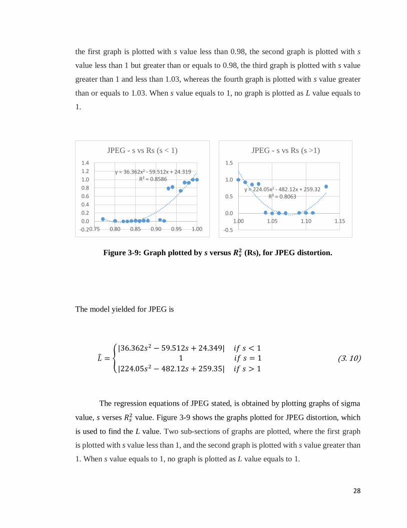
Figure 3-9: Graph plotted by s versus 𝑹𝒔𝟐 (Rs), for JPEG distortion.
The model yielded for JPEG is
�� = {
|36.362𝑠2 − 59.512𝑠 + 24.349| 𝑖𝑓 𝑠 < 1 1 𝑖𝑓 𝑠 = 1
|224.05𝑠2 − 482.12𝑠 + 259.35| 𝑖𝑓 𝑠 > 1
(3. 10)
The regression equations of JPEG stated, is obtained by plotting graphs of sigma
value, s verses 𝑅𝑠2 value. Figure 3-9 shows the graphs plotted for JPEG distortion, which
is used to find the L value. Two sub-sections of graphs are plotted, where the first graph
is plotted with s value less than 1, and the second graph is plotted with s value greater than
1. When s value equals to 1, no graph is plotted as L value equals to 1.
y = 36.362x2 - 59.512x + 24.319R² = 0.8586
-0.2
0.0
0.2
0.4
0.6
0.8
1.0
1.2
1.4
0.75 0.80 0.85 0.90 0.95 1.00
JPEG - s vs Rs (s < 1)
y = 224.05x2 - 482.12x + 259.32R² = 0.8063
-0.5
0.0
0.5
1.0
1.5
1.00 1.05 1.10 1.15
JPEG - s vs Rs (s >1)

29
Figure 3-10: Graph plotted by s versus 𝑹𝒔𝟐 (Rs), for JPEG2000 distortion.
The model yielded for JPEG2000 is
�� =
{
|0.2167𝑠 − 0.2366| 𝑖𝑓 𝑠 < 0.95|27.832𝑠 − 26.633| 𝑖𝑓 0.95 ≤ 𝑠 < 1
1 𝑖𝑓 𝑠 = 1|−4.8484𝑠 + 5.8739| 𝑖𝑓 1 < 𝑠 ≤ 1.03
|359.87𝑠2 − 773.64𝑠 + 415.73| 𝑖𝑓 𝑠 > 1.03
(3. 11)
The regression equations of JPEG2000 stated, is obtained by plotting graphs of
sigma value, s verses 𝑅𝑠2 value. Figure 3-10 shows the graphs plotted for JPEG2000
y = 0.2167x - 0.1766R² = 0.2773
-0.020000
0.000000
0.020000
0.040000
0.060000
0.080000
0.00 0.20 0.40 0.60 0.80 1.00
JPEG2k - s vs Rs (s < 0.95)
y = 27.832x - 26.573R² = 0.7217
-0.200000
0.000000
0.200000
0.400000
0.600000
0.800000
1.000000
1.200000
0.94 0.95 0.96 0.97 0.98 0.99 1.00
JPEG2k - s vs Rs (0.95 ≤ s < 1)
y = -4.8484x + 5.8139R² = 0.7714
0.000000
0.200000
0.400000
0.600000
0.800000
1.000000
1.200000
0.98 0.99 1.00 1.01 1.02 1.03 1.04
JPEG2k - s vs Rs (1 < s <1.03)
y = 359.87x2 - 773.64x + 415.67R² = 0.6815
-0.200000
0.000000
0.200000
0.400000
0.600000
0.800000
1.000000
1.02 1.04 1.06 1.08 1.10 1.12
JPEG2k - s vs Rs ( s ≥ 1.03)

30
distortion, which is used to find the L value. Four sub-sections of graphs are plotted, where
the first graph is plotted with s value less than 0.95, the second graph is plotted with s
value less than 1 but greater than or equals to 0.95, the third graph is plotted with s value
greater than 1 and less than 1.03, whereas the fourth graph is plotted with s value greater
than or equals to 1.03. When s value equals to 1, no graph is plotted as L value equals to
1.
3-5 Measuring the performance of IQM
A RR-IQA metrics is categorized as a good metrics when it satisfy three main properties,
which are monotonicity, consistency, and accuracy. The monotonicity property can be
judged by calculating the value of SRCC and KRCC. PLCC, MAE, and RMS are used to
determine the accuracy of a RR-IQA metric. The consistency can be determined by
observing the pattern of the graph plotted for results of different IQM. Therefore, a better
IQA metric should have higher PLCC, SRCC and KRCC while lower MAE and RMS
values.
3-5-1 Pearson linear correlation coefficient (PLCC)
Pearson linear correlation coefficient (PLCC), which was proposed by Karl Pearson from
a related idea introduced by Francis Galton in the 1880s, is used to measure the strength
of a linear relationship between two variables. The value of PLCC is always between -1
to 1. The linear relationship is strong when PLCC value is close to either -1 or 1, and is

31
weak when close to 0. There is no linear relationship when PLCC value is 0. The positive
and negative sign indicate the direction of the linear relationship. PLCC is defined as
𝑃𝐿𝐶𝐶 = ∑ (𝑞𝑖 −𝑖 𝑞 ) ∗ (𝑜𝑖 − 𝑜 )
√∑ (𝑞𝑖 −𝑖 ��)2 ∗ ∑ (𝑜𝑖 −𝑖 ��)2
where 𝑜𝑖 is the DMOS between reference and distorted images, and 𝑞𝑖 is a nonlinear
function.
3-5-2 Mean absolute error (MAE)
Mean absolute error (MAE) measures the average magnitude of errors in a set of
estimation. The MAE is the average of absolute errors between a prediction and the true
value, which in this study is between the reference image and distorted image. MAE is
defined with an equation as follow
𝑀𝐴𝐸 = 1
𝑁∑|𝑞𝑖 − 𝑜𝑖|

32
3-5-3 Root mean-squared (RMS) error
Root mean-squared (RMS) error is the square root of the average of the square of all error.
It is often used to measure the differences between the predicted values of a model and the
actually observed value. RMS can be defined as
𝑅𝑀𝑆 = √1
𝑁∑(𝑞𝑖 − 𝑜𝑖)2
3-5-4 Spearman’s rank correlation coefficient (SRCC)
The Spearman’s rank correlation coefficient (SRCC) is used to measure the strength of
the relationship between two sets of data. It is suitable for both discrete and continuous
data. The SRCC is defined as
𝑆𝑅𝐶𝐶 = 1 − 6∑ 𝑑𝑖
2𝑁𝑖=1
𝑁(𝑁2 − 1)
where 𝑑𝑖 is the difference between 𝑖 -th image’s ranks in subjective and objective
evaluations.

33
3-5-5 Kendall’s rank correlation coefficient (KRCC)
The Kendall (1955) rank correlation coefficient is another non-parametric rank correlation
metric that determine the similarity between two sets of rank given to same set of objects.
The KRCC is given by
𝐾𝑅𝐶𝐶 = 𝑁𝑐 −𝑁𝑑
1
2𝑁(𝑁 − 1)
where 𝑁𝑐 and 𝑁𝑑 are the numbers of consistent and inconsistent pairs in the data set,
respectively.
3-6 Bit Rate of Distortions
In visual data and computing, the number of bits that are transmitted or processed per unit
of time is called the bit rate. The bit rate is defined by calculating bits for each second.
LIVE database provided each distortions with different bit rate. The higher the bit rate of
distortion, the lower the quality of the image.
Different distortion has different range of bit rate value provided in LIVE database.
Gaussian Blur has bit rate value between 0 and 14.9997. JPEG has bit rate value between
0 and 3.3336. The bit rate value of JPEG2000 is between 0 and 3.1539. Gaussian Noise
has bit rate value between 0 and 1.9961, whereas Fast Fading has bit rate between 0 and
26.1. With different range of bit rate value given, we can say that if the bit rate value is
near to 0, the distortion of distorted image is considered non-noticeable, which means that
the quality of distorted image is relatively high.

34
CHAPTER 4
RESULTS AND DISCUSSION
Three different distortion types of imperfect reference image are used to test the image
quality assessment metrics proposed. They are Gaussian Blur distortion, JPEG distortion,
and JPEG2000 distortion. The sample data of Fast Fading distortion, and Gaussian Noise
distortion type used as imperfect reference image are not included in this report, which is
due to the inaccuracy of the L value obtained. The distorted images used are with different
bit rate, which included a total of five types of distortion.
The table records the results of each pair of reference image and distorted images
tested on each metrics used. Other than the RR-IQM proposed 𝑅𝐿2 (RL), there are five
other metrics that are involved in this study which used to make comparison. They are
SSIM, PSNR, 𝑅𝑠2 (Rs), estimated SSIM S (S_Dn), and DMOS value, which is given in
LIVE database.

35
4-1 Performance of 𝑹𝑳𝟐 When Reference Image Has Gaussian Blur Distortion
Here, Gaussian Blur distorted image is used as imperfect reference image. In order to test
the accuracy, consistency, and monotonicity of each of the RR-IQA applied to this
distortion type of reduced reference image, different types of distorted image is tested with
it. There are four types of distorted image being tested, which are JPEG, JPEG2000,
Gaussian Noise, and Fast Fading distortion.
4-1-1 JPEG distorted image as compressed image
Table 4-1(a) used a perfect quality image as the reference while (b), (c), (d), (e) and (f)
used a JPEG distorted image as the reference image. The bit rate of distortion increases
from (b) to (f). The result value more than one is converted to one in this table. This is
because the highest value qualified is one. From Table 4-1, we can see that the SSIM,𝑅𝐹2,
PSNR, and 𝑅𝐿2 value is decreasing gradually from (a) to (f).
SSIM is a metric designed for full reference image quality assessment. The value
of SSIM decreases from (a) to (f) indicates that SSIM value is less effective when the
reference image used has no perfect quality, and the bit rate of distortion increases.
The PSNR value decreases in value from (a) to (f). This is because PSNR is
calculated by the mean square error of the two images involved. When the reference image
is distorted, it could hardly give an accurate image quality assessment result.

36
Table 4-1: Results of each metrics applied on a JPEG distorted image, caps.bmp,
with different level of bit rate. The imperfect reference image used is with Gaussian
blur distortion. (a)Perfect quality image as reference. (b)Gaussian blur distorted
image with bit rate 0.677051 as reference. (c)Gaussian blur distorted image with bit
rate 1.164031 as reference. (d) Gaussian blur distorted image with bit rate 1.708303
as reference. (e) Gaussian blur distorted image with bit rate 3.083306 as reference.
(f) Gaussian blur distorted image with bit rate 5.833312 as reference.
Bit Rate of G.Blur = 0
Bit Rate SSIM PSNR S_Dn Rs L RL DMOS
0 1 65535 0.955331 1 1 1 100
0.15312 0.75055 25.86641 0.809367 0.944352 0.91461 1 60.06954
0.1993 0.838527 29.4221 0.864707 0.975457 0.959459 1 49.85666
0.40535 0.956837 34.09477 0.930092 0.991667 1.022811 0.969551 40.20038
0.42483 0.960829 34.36081 0.930826 0.99216 1.022606 0.970228 42.87448
0.85118 0.989243 38.29867 0.900567 0.99684 1.047553 0.951589 28.3078
(a)
Bit Rate of G.Blur = 0.677051
Bit Rate SSIM PSNR S_Dn Rs L RL DMOS
0 0.98811 36.16914 0.954758 0.994885 1.049929 0.947574 100
0.15312 0.777268 26.79641 0.980614 0.95442 0.973515 0.980385 60.06954
0.1993 0.85596 30.83819 0.990581 0.982025 1.018688 0.96401 49.85666
0.40535 0.958556 34.85438 0.957608 0.992961 1.077901 0.921199 40.20038
0.42483 0.961855 34.96304 0.955887 0.993128 1.078035 0.92124 42.87448
0.85118 0.982217 35.7065 0.932128 0.994261 1.050922 0.946084 28.3078
(b)
Bit Rate of G.Blur = 1.164031
Bit Rate SSIM PSNR S_Dn Rs L RL DMOS
0 0.955954 31.70434 0.951516 0.985561 1.000461 0.985107 100
0.15312 0.79836 27.09293 0.999389 0.957153 0.998243 0.958838 60.06954
0.1993 0.857682 30.47073 0.99869 0.980376 1.043551 0.939462 49.85666
0.40535 0.93781 32.0805 0.953872 0.986649 1.050719 0.939023 40.20038
0.42483 0.940243 32.06473 0.952134 0.986584 1.051032 0.938681 42.87448
0.85118 0.953256 31.80884 0.932489 0.985841 1.002024 0.98385 28.3078
(c)
Bit Rate of G.Blur = 1.708303
Bit Rate SSIM PSNR S_Dn Rs L RL DMOS
0 0.919171 29.76012 0.920504 0.97731 1.002991 0.974396 100

37
0.15312 0.80847 27.00901 0.999761 0.956145 0.997198 0.958831 60.06954
0.1993 0.845062 29.52151 0.996447 0.975542 1.0425 0.935772 49.85666
0.40535 0.906951 30.18129 0.92381 0.979265 1.052305 0.93059 40.20038
0.42483 0.908739 30.15227 0.921105 0.979098 1.052611 0.930162 42.87448
0.85118 0.917651 29.87137 0.890639 0.977797 1.004531 0.973387 28.3078
(d)
Bit Rate of G.Blur = 3.083306
Bit Rate SSIM PSNR S_Dn Rs L RL DMOS
0 0.852187 27.54849 0.861114 0.96207 0.892852 1 100
0.15312 0.800037 26.26837 0.999473 0.947724 1.033336 0.91715 60.06954
0.1993 0.802469 27.67737 0.993017 0.962494 1.080058 0.891149 49.85666
0.40535 0.844566 27.86098 0.867038 0.964481 0.974968 0.989243 40.20038
0.42483 0.845674 27.84127 0.862382 0.964275 0.975538 0.988455 42.87448
0.85118 0.851185 27.63827 0.809443 0.962708 0.89523 1 28.3078
(e)
Bit Rate of G.Blur = 5.833312
Bit Rate SSIM PSNR S_Dn Rs L RL DMOS
0 0.769698 25.25396 0.786669 0.935269 1.026541 0.911088 100
0.15312 0.752876 24.70845 0.999114 0.924701 0.8933 1 60.06954
0.1993 0.734077 25.42786 0.989045 0.936735 0.938032 0.998618 49.85666
0.40535 0.764098 25.45758 0.795599 0.93787 1.001218 0.936729 40.20038
0.42483 0.764841 25.44907 0.788459 0.937682 1.001014 0.936733 42.87448
0.85118 0.768765 25.32062 0.707046 0.936031 1.025895 0.912404 28.3078
(f)
Besides, the value of 𝑅𝑠2 and 𝑅𝐿
2 also show a decrease from Table 4-1(a) to (f).
However, the decreasing of the average value is small. The distortion is non-noticeable
because the bit rate of distorted image is relatively small, which indicates that the distorted
image is considered high quality. Therefore, the result value is close to 1 although the bit
rate is the highest here. This shows that both 𝑅𝑠2 and 𝑅𝐿
2 are suitable for reduced reference
image quality assessment. However, from (f), we can see that 𝑅𝐿2 provided a better result
than𝑅𝑠2.
The S value calculated from 𝐷𝑛 value has inconsistent changes in value, as we can
see from Table 4-1 (a) to (f).The S values increase while some decrease inconsistently.

38
This indicates that the estimated SSIM, S is inaccurate and ineffective for reduced
reference image quality assessment.
As what we can see in Table 4-1 (f), the value of each metric results is
inconsistently small. This indicates that an imperfect reference image with a higher bit
rate of distortion will affect the accuracy of a RR-IQA. However, the results for 𝑅𝐿2
decrease in a consistent way.
Table 4-2: Results of each metrics used to judge the performance of RR-IQA metrics
used.
Bit Rate PLCC MAE RMSE SRCC KRCC
DMOS vs
SSIM
0 0.018983 53.55148 57.39575 -0.08571 -0.2
0.677051 -0.00584 53.55148 57.39232 -0.08571 -0.2
1.164031 -0.02299 53.55148 57.40499 -0.08571 -0.2
1.708303 -0.02322 53.55148 57.42581 -0.08571 -0.2
3.083306 0.013123 53.55148 57.47266 -0.08571 -0.2
5.833312 0.100773 53.55148 57.53982 -0.02857 -0.06667
DMOS vs
S_Dn
0 0.203077 53.55148 57.40849 0.085714 0.066667
0.677051 0.213667 53.55148 57.35263 0.314286 0.2
1.164031 0.166832 53.55148 57.35004 0.371429 0.333333
1.708303 0.166157 53.55148 57.36977 0.371429 0.333333
3.083306 0.165412 53.55148 57.40751 0.371429 0.333333
5.833312 0.166106 53.55148 57.45493 0.371429 0.333333
DMOs vs
Rs
0 0.001028 53.55148 57.33454 -0.08571 -0.2
0.677051 -0.07851 53.55148 57.33329 -0.08571 -0.2
1.164031 -0.1364 53.55148 57.33793 -0.65714 -0.46667
1.708303 -0.16844 53.55148 57.34355 -0.65714 -0.46667
3.083306 -0.20817 53.55148 57.35593 -0.77143 -0.6
5.833312 -0.24557 53.55148 57.37965 -0.6 -0.46667
DMOS vs
RL
0 0.74185 53.55148 57.33029 0.941124 0.894427
0.677051 0.281114 53.55148 57.36578 0.657143 0.466667
1.164031 0.408432 53.55148 57.35501 0.371429 0.333333
1.708303 0.428249 53.55148 57.36144 0.371429 0.333333
3.083306 0.021625 53.55148 57.35169 -0.23191 -0.27603
5.833312 -0.07774 53.55148 57.36702 0.142857 0.333333
39
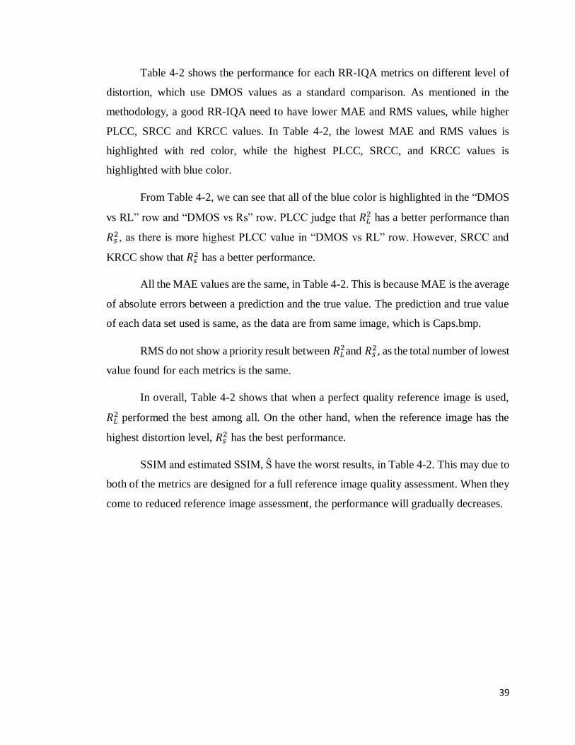
Table 4-2 shows the performance for each RR-IQA metrics on different level of
distortion, which use DMOS values as a standard comparison. As mentioned in the
methodology, a good RR-IQA need to have lower MAE and RMS values, while higher
PLCC, SRCC and KRCC values. In Table 4-2, the lowest MAE and RMS values is
highlighted with red color, while the highest PLCC, SRCC, and KRCC values is
highlighted with blue color.
From Table 4-2, we can see that all of the blue color is highlighted in the “DMOS
vs RL” row and “DMOS vs Rs” row. PLCC judge that 𝑅𝐿2 has a better performance than
𝑅𝑠2, as there is more highest PLCC value in “DMOS vs RL” row. However, SRCC and
KRCC show that 𝑅𝑠2 has a better performance.
All the MAE values are the same, in Table 4-2. This is because MAE is the average
of absolute errors between a prediction and the true value. The prediction and true value
of each data set used is same, as the data are from same image, which is Caps.bmp.
RMS do not show a priority result between 𝑅𝐿2and 𝑅𝑠
2, as the total number of lowest
value found for each metrics is the same.
In overall, Table 4-2 shows that when a perfect quality reference image is used,
𝑅𝐿2 performed the best among all. On the other hand, when the reference image has the
highest distortion level, 𝑅𝑠2 has the best performance.
SSIM and estimated SSIM, S have the worst results, in Table 4-2. This may due to
both of the metrics are designed for a full reference image quality assessment. When they
come to reduced reference image assessment, the performance will gradually decreases.

40
Figure 4-1: Graph plotted by IQM results versus bit rate of imperfect reference
image. It is to show the relationship of each metrics, with different bit rate value of
JPEG distorted value, and different level of distortion for Gaussian blur distorted
reference image.
00.20.40.60.8
11.2
G.Blur vs JPEG
(bit rate = 0)
SSIM S_Dn Rs RL
0
0.2
0.4
0.6
0.8
1
1.2
1 2 3 4 5 6
G.Blur vs JPEG
(bit rate = 0.15312)
SSIM S_Dn Rs RL
00.20.40.60.8
11.2
G.Blur vs JPEG
(bit rate = 0.1993)
SSIM S_Dn Rs RL
00.20.40.60.8
11.2
G.Blur vs JPEG
(bit rate = 0.85118)
SSIM S_Dn Rs RL
00.20.40.60.8
11.2
G.Blur vs JPEG
(bit rate = 0.40535)
SSIM S_Dn Rs RL
00.20.40.60.8
11.2
G.Blur vs JPEG
(bit rate = 0.42483)
SSIM S_Dn Rs RL

41
In Figure 4-1, it shows the graph plotted for each metrics with different bit rate
value of distortion. The graph is used to show the performance of each metrics when the
bit rate value of JPEG distorted image is increasing in each graph, and the Gaussian blur
imperfect reference image has different distortion value, which is in x-axis. The flatter the
pattern of the graph, indicates a better consistency of the IQM tested.
From Figure 4-1, 𝑅𝐿2 has a better performance as compared to other metrics, when
JPEG distorted image has a perfect quality or with bit rate 0 and 0.15312. For other JPEG
distorted image, 𝑅𝑠2 has an average of better consistency. Here, we can say that 𝑅𝐿
2 and
𝑅𝑠2provide a more consistent assessment to Gaussian blur distorted reduced reference
image.
In overall, the performance of 𝑅𝑠2 and 𝑅𝐿
2 are the best when compared to the other
metrics included, when the reference image has Gaussian blur distortion is compared to
JPEG distorted image.
4-1-2 JPEG2000 distorted image as compressed image
Table 4-3(a) used a perfect quality image as the reference while (b), (c), (d), (e) and (f)
used a JPEG2000 distorted image as the reference image. The bit rate of distortion
increases from (b) to (f). The result value more than one is converted to one in this table.
This is because the highest value qualified is one. From Table 4-3, we can see that the
SSIM,𝑅𝐹2, PSNR, and 𝑅𝐿
2 value is decreasing gradually from (a) to (f).
SSIM is a metric designed for full reference image quality assessment. The value
of SSIM decreases from (a) to (f) for each of the different bit rate for Gaussian blur
reference image. This indicates that SSIM value is less effective when the reference image
used has no perfect quality, and the bit rate of distortion increases.

42
The PSNR value decreases in value from (a) to (f). This is because PSNR is
calculated by the mean square error of the two images involved. When the reference image
is distorted, it could hardly give an accurate image quality assessment result.
Table 4-3: Results of each metrics applied on a JPEG2000 compressed image,
caps.bmp, with different level of bit rate. The imperfect reference image used is with
Gaussian Blur distortion. (a)Perfect quality image as reference. (b)Gaussian Blur
distorted image with bit rate 0.677051 as reference. (c)Gaussian Blur distorted image
with bit rate 1.164031 as reference. (d)Gaussian Blur distorted image with bit rate
1.708303 as reference. (e)Gaussian Blur distorted image with bit rate 3.083306 as
reference. (f)Gaussian Blur distorted image with bit rate 5.833312 as reference.
Bit Rate of G.Blur = 0
Bit Rate SSIM PSNR S_Dn Rs L RL DMOS
0 1 65535 0.968702 1 1 1 100
0.050378 0.831895 28.98727 0.845755 0.972697 0.941349 1 56.81507
0.098741 0.889199 30.8188 0.928655 0.982177 0.966907 1 53.4561
0.19944 0.929898 33.27789 0.945545 0.989921 0.990785 0.999128 46.58432
0.40137 0.964494 36.69453 0.931831 0.995423 1.031065 0.965432 34.49728
0.60354 0.977638 39.26188 0.936601 0.997469 1.043332 0.956042 26.6733
(a)
Bit Rate of G.Blur = 0.677051
Bit Rate SSIM PSNR S_Dn Rs L RL DMOS
0 0.98811 36.16914 0.962885 0.994885 1.049929 0.947574 100
0.050378 0.867478 31.23329 0.976932 0.983349 1.000447 0.982909 56.81507
0.098741 0.918368 33.20056 0.991017 0.989481 1.026189 0.964229 53.4561
0.19944 0.946333 34.63151 0.973474 0.992504 1.08101 0.918127 46.58432
0.40137 0.968186 35.52851 0.946538 0.993978 1.071281 0.927841 34.49728
0.60354 0.975993 35.71695 0.943858 0.994272 1.05704 0.94062 26.6733
(b)
Bit Rate of G.Blur = 1.164031
Bit Rate SSIM PSNR S_Dn Rs L RL DMOS
0 0.955954 31.70434 0.954946 0.985561 1.000461 0.985107 100
0.050378 0.898963 32.2477 0.995877 0.986668 1.025255 0.962364 56.81507
0.098741 0.934541 33.02777 0.991214 0.989003 1.081382 0.914574 53.4561
0.19944 0.944068 32.62334 0.966312 0.988091 1.081746 0.913422 46.58432

43
0.40137 0.951464 32.14243 0.941224 0.986833 1.036868 0.951744 34.49728
0.60354 0.953583 31.86576 0.937583 0.986025 1.011855 0.974472 26.6733
(c)
Bit Rate of G.Blur = 1.708303
Bit Rate SSIM PSNR S_Dn Rs L RL DMOS
0 0.919171 29.76012 0.93078 0.97731 1.002991 0.974396 100
0.050378 0.918336 32.15909 0.995143 0.986341 1.024207 0.963028 56.81507
0.098741 0.934333 31.81161 0.984653 0.98545 1.08091 0.911686 53.4561
0.19944 0.928354 30.87118 0.946939 0.98215 1.08215 0.907592 46.58432
0.40137 0.925222 30.23945 0.910937 0.979535 1.038761 0.942984 34.49728
0.60354 0.923177 29.95207 0.905541 0.978209 1.014205 0.964509 26.6733
(d)
Bit Rate of G.Blur = 3.083306
Bit Rate SSIM PSNR S_Dn Rs L RL DMOS
0 0.852187 27.54849 0.879018 0.96207 0.892852 1 100
0.050378 0.919728 30.31181 0.99142 0.979146 1.08391 0.903347 56.81507
0.098741 0.903194 29.2993 0.972439 0.974056 1.075095 0.906019 53.4561
0.19944 0.882801 28.44585 0.906914 0.96873 1.045904 0.926213 46.58432
0.40137 0.868323 27.92243 0.844752 0.964981 0.950781 1 34.49728
0.60354 0.861787 27.69965 0.835396 0.963244 0.91037 1 26.6733
(e)
Bit Rate of G.Blur = 5.833312
Bit Rate SSIM PSNR S_Dn Rs L RL DMOS
0 0.769698 25.25396 0.806571 0.935269 1.026541 0.911088 100
0.050378 0.867239 27.14056 0.98622 0.956737 0.919969 1 56.81507
0.098741 0.82954 26.35671 0.955657 0.948726 0.94546 1 53.4561
0.19944 0.807126 25.83444 0.850843 0.942673 0.969276 0.972554 46.58432
0.40137 0.789069 25.49545 0.751564 0.93842 1.009451 0.929634 34.49728
0.60354 0.780574 25.35055 0.736621 0.936494 1.021686 0.916617 26.6733
(f)
The value of 𝑅𝑠2 also show a decrease from Table 4-3(a) to (f). However, the
decreasing of the average value is small. This shows that 𝑅𝑠2 is suitable for reduced
reference image quality assessment. On the other hand, the values of 𝑅𝐹2 fluctuated
inconsistently from Table 4-3 (a) to (f). However, from (f), we can see that 𝑅𝐿2 provided a
better result than𝑅𝑠2 in overall. The distortion is non-noticeable because the bit rate of

44
distorted image is relatively small, which indicates that the distorted image is considered
high quality. Therefore, the result value is close to 1 although the bit rate is the highest
here.
The S value calculated from 𝐷𝑛 value decreases in overall, as we can see from
Table 4-3 (a) to (f). However, the S value is less than the value of 𝑅𝑠2 and 𝑅𝐹
2 in general.
This indicates that the estimated SSIM, S is less accurate and less effective for this
assessment.
As what we can see in Table 4-3 (f), the value of each metric results is smaller than
the previous results. This means that a Gaussian blur distorted reference image with a
higher bit rate of JPEG2000 distortion will affect the accuracy of a RR-IQA. However,
the results for 𝑅𝐿2has the highest value among all metrics.
Table 4-4 shows the performance for each RR-IQA metrics on different level of
distortion, which use DMOS values as a standard comparison. As mentioned in the
methodology, a good RR-IQA need to have lower MAE and RMS values, and higher
PLCC, SRCC and KRCC values. In Table 4-4, the lowest MAE and RMS values is
highlighted with red color, while the highest PLCC, SRCC, and KRCC values is
highlighted with blue color.
From Table 4-4, we can see that most of the blue color is highlighted in the “DMOS
vs S_Dn” row and the second most is highlighted in “DMOS vs RL” row. PLCC judge
that the estimated SSIM, S has a better performance, as there are more highest PLCC value
in “DMOS vs RL” row. Besides, SRCC and KRCC also show that estimated SSIM, S has
a better performance.
All the MAE values are the same in Table 4-4. This is because MAE is the average
of absolute errors between a prediction and the true value. The prediction and true value
of each data set used is same, as the data are from same image, which is Caps.bmp. RMS
shows a priority result in 𝑅𝑠2, as the total number of lowest value found in “DMOS vs Rs”
row is the largest.

45
Table 4-4: Results of each metrics used to judge the performance of RR-IQA
metrics used.
Bit Rate PLCC MAE RMSE SRCC KRCC
DMOS vs
SSIM
0 0.124935 53.00435 57.10726 -0.14286 -0.33333
0.677051 0.080613 53.00435 57.09798 -0.14286 -0.33333
1.164031 -0.00182 53.00435 57.10328 -0.14286 -0.33333
1.708303 -0.35411 53.00435 57.11773 -0.37143 -0.06667
3.083306 -0.1405 53.00435 57.1579 0.142857 0.333333
5.833312 -0.10464 53.00435 57.22557 0.142857 0.333333
DMOS vs
S_Dn
0 0.220785 53.00435 57.11218 0.028571 -0.06667
0.677051 0.340524 53.00435 57.0772 0.6 0.466667
1.164031 0.255097 53.00435 57.07832 0.657143 0.6
1.708303 0.249044 53.00435 57.09439 0.657143 0.6
3.083306 0.24815 53.00435 57.12895 0.657143 0.6
5.833312 0.248973 53.00435 57.1774 0.657143 0.6
DMOs vs
Rs
0 0.077527 53.00435 57.05751 -0.14286 -0.33333
0.677051 0.003202 53.00435 57.05617 -0.14286 -0.33333
1.164031 -0.27829 53.00435 57.0603 -0.2 -0.06667
1.708303 -0.11888 53.00435 57.06538 0.142857 0.333333
3.083306 -0.06619 53.00435 57.07704 0.142857 0.333333
5.833312 -0.04709 53.00435 57.10041 0.142857 0.333333
DMOS vs
RL
0 0.688516 53.00435 57.05514 0.941124 0.894427
0.677051 0.2879 53.00435 57.0942 0.6 0.333333
1.164031 0.318734 53.00435 57.09006 0.257143 0.2
1.708303 0.326821 53.00435 57.09587 0.257143 0.2
3.083306 0.010016 53.00435 57.08835 -0.39466 -0.44721
5.833312 -0.09579 53.00435 57.09087 0.115954 0.276026
In overall, Table 4-4 shows that when a perfect quality reference image is used,
𝑅𝐿2 performed the best among all. On the other hand, when the reference image has the
highest distortion level, the estimated SSIM, S has the best performance.
SSIM have the worst results, in Table 4-4. This may due to it is designed for a full
reference image quality assessment. When it comes to reduced reference image quality
assessment, the performance will gradually decreases.
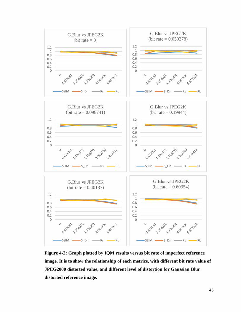
46
Figure 4-2: Graph plotted by IQM results versus bit rate of imperfect reference
image. It is to show the relationship of each metrics, with different bit rate value of
JPEG2000 distorted value, and different level of distortion for Gaussian Blur
distorted reference image.
00.20.40.60.8
11.2
G.Blur vs JPEG2K
(bit rate = 0)
SSIM S_Dn Rs RL
00.20.40.60.8
11.2
G.Blur vs JPEG2K
(bit rate = 0.050378)
SSIM S_Dn Rs RL
00.20.40.60.8
11.2
G.Blur vs JPEG2K
(bit rate = 0.098741)
SSIM S_Dn Rs RL
00.20.40.60.8
11.2
G.Blur vs JPEG2K
(bit rate = 0.19944)
SSIM S_Dn Rs RL
00.20.40.60.8
11.2
G.Blur vs JPEG2K
(bit rate = 0.40137)
SSIM S_Dn Rs RL
00.20.40.60.8
11.2
G.Blur vs JPEG2K
(bit rate = 0.60354)
SSIM S_Dn Rs RL

47
In Figure 4-2, it shows the graph plotted for each metrics with different bit rate
value of distortion. The graph is used to show the performance of each metrics when the
bit rate value of JPEG2000 distorted image is increasing in each graph, and the Gaussian
blur distorted reference image has different distortion value, which is in x-axis of the graph.
The flatter the pattern of the graph, indicates a better consistency of the IQM tested.
From Figure 4-2, 𝑅𝑠2 has a better consistency as compared to other metrics, when
JPEG distorted image is used as the reference image, followed by 𝑅𝐿2, Here, we can say
that 𝑅𝑠2 provide a more accurate assessment to higher level of Gaussian blur reduced
reference image.
In overall, the performance of the 𝑅𝑠2 are the best as compared to the other metrics
included, when the reference image has Gaussian blur distortion is compared to JPEG2000
distorted image.
4-1-3 Gaussian Noise distorted image as compressed image
Table 4-5(a) shows the use of a perfect quality image as the reference while (b), (c), (d),
(e) and (f) used a Gaussian blur distorted image as the reference image. The bit rate of
distortion increases from (b) to (f). The result value more than one is converted to one in
this table. This is because the highest value qualified is one. From Table 4-5, we can see
that the SSIM, 𝑅𝐹2, PSNR, and 𝑅𝐿
2 value is decreasing gradually from (a) to (f).
SSIM is a metric designed for full reference image quality assessment. The value
of SSIM decreases from (a) to (f) for each of the different bit rate for Gaussian blur
reference image. This indicates that SSIM value is less effective when the reference image
used has no perfect quality, and the bit rate of distortion increases.

48
The PSNR value decreases in value from (a) to (f). This is because PSNR is
calculated by the mean square error of the two images involved. When the reference image
is distorted, it could hardly give an accurate image quality assessment result.
Table 4-5: Results of each metrics applied on Gaussian Noise distorted image,
caps.bmp. (a)Perfect quality image as reference. (b)Gaussian Blur distorted image
with bit rate 0.677051 as reference. (c)Gaussian Blur distorted image with bit rate
1.164031 as reference. (d)Gaussian Blur distorted image with bit rate 1.708303 as
reference. (e)Gaussian Blur distorted image with bit rate 3.083306 as reference.
(f)Gaussian Blur distorted image with bit rate 5.833312 as reference.
Bit Rate of G.Blur = 0
Bit Rate SSIM PSNR S_Dn Rs L RL DMOS
0 1 65535 0.948758 1 1 1 100
0.015625 0.982878 39.55768 0.95635 0.997643 1.037724 0.961376 22.50337
0.03125 0.937012 33.61711 0.884508 0.990815 1.002782 0.988066 33.54177
0.0625 0.801863 27.65342 0.747118 0.964984 0.909943 1 41.3394
0.125 0.548208 21.75995 0.60953 0.87853 0.746509 1 48.03932
1 0.086885 10.31411 0.086594 0.198253 0.14375 1 67.38191
(a)
Bit Rate of G.Blur = 0.677051
Bit Rate SSIM PSNR S_Dn Rs L RL DMOS
0 0.98811 36.16914 0.825551 0.994885 1.049929 0.947574 100
0.015625 0.970982 34.56806 0.947825 0.992588 1.064204 0.932705 22.50337
0.03125 0.924787 31.74925 0.934237 0.985874 1.084049 0.909436 33.54177
0.0625 0.787781 27.10482 0.842322 0.96018 0.968815 0.991087 41.3394
0.125 0.533796 21.62159 0.686164 0.874204 0.837226 1 48.03932
1 0.084027 10.32709 0.054933 0.197344 0.176888 1 67.38191
(b)
Bit Rate of G.Blur = 1.164031
Bit Rate SSIM PSNR S_Dn Rs L RL DMOS
0 0.955954 31.70434 0.646223 0.985561 1.000461 0.985107 100
0.015625 0.938991 31.07492 0.848326 0.98332 1.023947 0.960323 22.50337
0.03125 0.893338 29.60307 0.895901 0.976737 1.074353 0.90914 33.54177
0.0625 0.757371 26.24962 0.872055 0.951309 0.993528 0.957506 41.3394
0.125 0.508428 21.37179 0.737976 0.866214 0.876948 0.987759 48.03932

49
1 0.080194 10.32946 0.13606 0.19558 0.192213 1 67.38191
(c)
Bit Rate of G.Blur = 1.708303
Bit Rate SSIM PSNR S_Dn Rs L RL DMOS
0 0.919171 29.76012 0.594467 0.97731 1.002991 0.974396 100
0.015625 0.902473 29.35532 0.815393 0.975121 1.026088 0.950328 22.50337
0.03125 0.857599 28.31999 0.875686 0.968631 1.075199 0.900885 33.54177
0.0625 0.723638 25.61696 0.867443 0.943476 0.992483 0.950622 41.3394
0.125 0.481207 21.16344 0.737645 0.859143 0.87525 0.981597 48.03932
1 0.07637 10.33121 0.145666 0.193957 0.191549 1 67.38191
(d)
Bit Rate of G.Blur = 3.083306
Bit Rate SSIM PSNR S_Dn Rs L RL DMOS
0 0.852187 27.54849 0.558907 0.96207 0.892852 1 100
0.015625 0.836078 27.31014 0.797405 0.959977 0.929507 1 22.50337
0.03125 0.792935 26.64351 0.863941 0.953639 1.023597 0.931655 33.54177
0.0625 0.663245 24.64884 0.857726 0.928985 1.028601 0.903154 41.3394
0.125 0.432563 20.80499 0.720564 0.84608 0.934989 0.904909 48.03932
1 0.069368 10.33642 0.090747 0.191011 0.215397 0.886787 67.38191
(e)
Bit Rate of G.Blur = 5.833312
Bit Rate SSIM PSNR S_Dn Rs L RL DMOS
0 0.769698 25.25396 0.520709 0.935269 1.026541 0.911088 100
0.015625 0.754361 25.11933 0.779552 0.933312 1.016093 0.918531 22.50337
0.03125 0.713773 24.71051 0.851599 0.927188 0.981241 0.944914 33.54177
0.0625 0.591 23.3458 0.84575 0.90342 0.888645 1 41.3394
0.125 0.375574 20.24025 0.698071 0.823054 0.715047 1 48.03932
1 0.060301 10.34148 0.016288 0.185731 0.132931 1 67.38191
(f)
The value of 𝑅𝑠2 also show a decrease from Table 4-5(a) to (f). However, the
decreasing of the average value is small. This shows that 𝑅𝑠2 is suitable for reduced
reference image quality assessment. On the other hand, the values of 𝑅𝐿2 fluctuated
inconsistently from Table 4-5(a) to (f). However, from (f), we can see that 𝑅𝐿2 provided a
better result than𝑅𝑠2 in overall, especially for the highest value of Gaussian Noise bit rate

50
value. The distortion is non-noticeable because the bit rate of distorted image is relatively
small, which indicates that the distorted image is considered high quality. Therefore, the
result value is close to 1 although the bit rate is the highest here.
The S value calculated from 𝐷𝑛 value decreases in overall, as we can see from
Table 4-5 (a) to (f). However, the S value is less than the value of 𝑅𝑠2 and 𝑅𝐹
2 in general.
This indicates that the estimated SSIM, S is less accurate and less effective for this
assessment.
As what we can see in Table 4-5 (f), the value of each metric results is smaller than
the previous results. This means that a Gaussian blur distorted reference image with a
higher bit rate of Gaussian Noise distortion will affect the accuracy of a RR-IQA. However,
the results for 𝑅𝐿2 has the highest value among all metrics.
Table 4-6 shows the performance for each RR-IQA metrics on different level of
distortion, which use DMOS values as a standard comparison. As mentioned in the
methodology, a good RR-IQA need to have lower MAE and RMS values, and higher
PLCC, SRCC and KRCC values. In Table 4-6, the lowest MAE and RMS values is
highlighted with red color, while the highest PLCC, SRCC, and KRCC values is
highlighted with blue color.
From Table 4-6, we can see that most of the blue color is highlighted in the “DMOS
vs S_Dn” row and the second most is highlighted in “DMOS vs RL” row. PLCC judge
that the estimated SSIM, S has a better performance, as there are more highest PLCC value
in “DMOS vs RL” row. Besides, SRCC and KRCC also show that estimated SSIM, S has
a better performance.
All the MAE values are the same in Table 4-4. This is because MAE is the average
of absolute errors between a prediction and the true value. The prediction and true value
of each data set used is same, as the data are from same image, which is Caps.bmp. On
the other hand, RMS shows a priority result in 𝑅𝐿2, as all of the lowest value found in
“DMOS vs RL” row.

51
Table 4-6: Results of each metrics used to judge the performance of RR-IQA metrics
used.
Bit Rate PLCC MAE RMSE SRCC KRCC
DMOS vs
SSIM
0 -0.16678 52.1343 57.37961 -0.14286 -0.33333
0.677051 -0.16462 52.1343 57.38914 -0.14286 -0.33333
1.164031 -0.16204 52.1343 57.4112 -0.14286 -0.33333
1.708303 -0.15938 52.1343 57.43593 -0.14286 -0.33333
3.083306 -0.15456 52.1343 57.48069 -0.14286 -0.33333
5.833312 -0.14884 52.1343 57.53523 -0.14286 -0.33333
DMOS vs
S_Dn
0 -0.1867 52.1343 57.39904 -0.42857 -0.46667
0.677051 -0.36244 52.1343 57.41475 -0.82857 -0.73333
1.164031 -0.53098 52.1343 57.44983 -0.77143 -0.6
1.708303 -0.57116 52.1343 57.46744 -0.77143 -0.6
3.083306 -0.5773 52.1343 57.49413 -0.77143 -0.6
5.833312 -0.57851 52.1343 57.52646 -0.77143 -0.6
DMOs vs
Rs
0 -0.25166 52.1343 57.2872 -0.14286 -0.33333
0.677051 -0.25176 52.1343 57.29079 -0.14286 -0.33333
1.164031 -0.25186 52.1343 57.29741 -0.14286 -0.33333
1.708303 -0.25194 52.1343 57.30327 -0.14286 -0.33333
3.083306 -0.25208 52.1343 57.3141 -0.14286 -0.33333
5.833312 -0.25227 52.1343 57.33319 -0.14286 -0.33333
DMOS vs
RL
0 0.631012 52.1343 57.11294 0.845154 0.774597
0.677051 0.233634 52.1343 57.13841 0.579771 0.414039
1.164031 0.585122 52.1343 57.13149 0.657143 0.466667
1.708303 0.561411 52.1343 57.13766 0.771429 0.6
3.083306 0.139721 52.1343 57.16228 -0.23191 -0.27603
5.833312 -0.13756 52.1343 57.14542 0.030359 0.149071
In overall, Table 4-6 shows that when a perfect quality reference image is used,
𝑅𝐿2 performed the best among all. On the other hand, when the reference image has the
highest distortion level, the estimated SSIM, S has the best performance.
SSIM have the worst results, in Table 4-6. This may due to it is designed for a full
reference image quality assessment. When it comes to reduced reference image quality
assessment, the performance will gradually decreases.

52
Figure 4-3: Graph plotted by IQM results versus bit rate of imperfect reference
image. It is to show the relationship of each metrics, with different bit rate value of
Gaussian Noise distorted value, and different level of distortion for Gaussian blur
distorted reference image.
00.20.40.60.8
11.2
G.Blur vs G. Noise
(bit rate = 0)
SSIM S_Dn Rs RL
00.20.40.60.8
11.2
G.Blur vs G. Noise
(bit rate = 0.015625)
SSIM S_Dn Rs RL
00.20.40.60.8
11.2
G.Blur vs G. Noise
(bit rate = 0.03125)
SSIM S_Dn Rs RL
00.20.40.60.8
11.2
G.Blur vs G. Noise
(bit rate = 0.0625)
SSIM S_Dn Rs RL
00.20.40.60.8
11.2
G.Blur vs G. Noise
(bit rate = 0.125)
SSIM S_Dn Rs RL
00.20.40.60.8
11.2
G.Blur vs G. Noise
(bit rate = 1)
SSIM S_Dn Rs RL
53
In Figure 4-3, it shows the graph plotted for each metrics with different bit rate
value of distortion. The graph is used to show the performance of each metrics when the
bit rate value of Gaussian Noise distorted image is increasing, and the Gaussian Blur
distorted reference image has different distortion value, which is in x-axis of the graph.
The flatter the pattern of the graph, indicates a better consistency of the IQM tested.
From Figure 4-3, 𝑅𝐿2 has a better consistency as compared to other metrics, for the
lower bit rate of Gaussian Noise distorted image. 𝑅𝑠2 has better consistency when the
Gaussian Noise distorted images has higher bit rate distortion. Here, we can say that 𝑅𝐿2
provide a consistent assessment to Gaussian Blur reduced reference image.
In overall, the performance of the 𝑅𝐿2 are the best as compared to the other metrics
included, when the reference image has Gaussian Blur distortion is compared to Gaussian
Boise distorted image.
4-1-4 Fast Fading distorted image as compressed image
Table 4-7(a) used a perfect quality image as the reference while (b), (c), (d), (e) and (f)
used a fast fading distorted image as the reference image. The bit rate of distortion
increases from (b) to (f). The result value more than one is converted to one in this table.
This is because the highest value qualified is one. From Table 4-7, we can see that the
SSIM, 𝑅𝐹2, PSNR, and 𝑅𝐿
2 value is decreasing gradually from (a) to (f).
SSIM is a metric designed for full reference image quality assessment. The value
of SSIM decreases from (a) to (f) for each of the different bit rate for Gaussian blur
reference image. This indicates that SSIM value is less effective when the reference image
used has no perfect quality, and the bit rate of distortion increases.

54
The PSNR value decreases in value from (a) to (f). This is because PSNR is
calculated by the mean square error of the two images involved. When the reference image
is distorted, it could hardly give an accurate image quality assessment result.
Table 4-7: Results of each metrics applied on a Fast Fading compressed image,
caps.bmp, with different level of bit rate. The imperfect reference image used is with
Gaussian blur distortion. (a)Perfect quality image as reference. (b)Gaussian Blur
distorted image with bit rate 0.677051 as reference. (c)Gaussian Blur distorted image
with bit rate 1.164031 as reference. (d) Gaussian Blur distorted image with bit rate
1.708303 as reference. (e)Gaussian Blur distorted image with bit rate 3.083306 as
reference. (f) Gaussian Blur distorted image with bit rate 5.833312 as reference.
Bit Rate of G.Blur = 0
Bit Rate SSIM PSNR S_Dn Rs L RL DMOS
0 1 65535 0.954867 1 1 1 100
15.5 0.729741 25.41353 0.784455 0.936684 0.92539 1 69.00739
18.9 0.796929 26.59974 0.803897 0.952255 0.930471 1 60.05539
20.3 0.910108 29.91208 0.88453 0.97799 0.924763 1 50.70893
23.7 0.98202 36.04244 0.945002 0.994681 1.014239 0.980716 34.45273
25.1 0.96702 34.6269 0.90351 0.99263 1.01404 0.978886 42.48964
(a)
Bit Rate of G.Blur = 0.677051
Bit Rate SSIM PSNR S_Dn Rs L RL DMOS
0 0.98811 36.16914 0.912767 0.994885 1.049929 0.947574 100
15.5 0.764491 26.51579 0.948952 0.949771 0.984373 0.964848 69.00739
18.9 0.833129 28.00254 0.956637 0.964688 0.989491 0.974933 60.05539
20.3 0.944741 33.11247 0.978407 0.989227 0.983742 1 50.70893
23.7 0.984926 36.77243 0.923807 0.995468 1.08225 0.919813 34.45273
25.1 0.969061 35.03805 0.917374 0.993262 1.082321 0.917715 42.48964
(b)
Bit Rate of G.Blur = 1.164031
Bit Rate SSIM PSNR S_Dn Rs L RL DMOS
0 0.955954 31.70434 0.943989 0.985561 1.000461 0.985107 100
15.5 0.801286 27.31611 0.995716 0.957627 1.009133 0.94896 69.00739
18.9 0.86886 28.91042 0.995693 0.970987 1.014266 0.95733 60.05539

55
20.3 0.966993 34.86271 0.990889 0.992741 1.0085 0.984374 50.70893
23.7 0.964167 33.07663 0.945665 0.989371 1.062561 0.931119 34.45273
25.1 0.947921 32.22648 0.949438 0.987112 1.062806 0.92878 42.48964
(c)
Bit Rate of G.Blur = 1.708303
Bit Rate SSIM PSNR S_Dn Rs L RL DMOS
0 0.919171 29.76012 0.913302 0.97731 1.002991 0.974396 100
15.5 0.835779 28.0476 0.995277 0.963743 1.008087 0.956013 69.00739
18.9 0.896704 29.48205 0.99436 0.974329 1.013219 0.961617 60.05539
20.3 0.967057 34.36271 0.983923 0.991876 1.007454 0.984538 50.70893
23.7 0.931709 30.83765 0.914271 0.982145 1.06383 0.923216 34.45273
25.1 0.915085 30.29871 0.920422 0.979852 1.064067 0.920855 42.48964
(d)
Bit Rate of G.Blur = 3.083306
Bit Rate SSIM PSNR S_Dn Rs L RL DMOS
0 0.852187 27.54849 0.844948 0.96207 0.892852 1 100
15.5 0.89601 29.34151 0.991894 0.972507 1.044272 0.931278 69.00739
18.9 0.915444 29.39612 0.989957 0.973594 1.080625 0.900954 60.05539
20.3 0.920787 30.94495 0.97062 0.982215 1.043637 0.941146 50.70893
23.7 0.866126 28.23367 0.846419 0.967349 0.997522 0.969753 34.45273
25.1 0.848799 27.91118 0.85685 0.964944 0.998014 0.966864 42.48964
(e)
Bit Rate of G.Blur = 5.833312
Bit Rate SSIM PSNR S_Dn Rs L RL DMOS
0 0.769698 25.25396 0.754604 0.935269 1.026541 0.911088 100
15.5 0.941385 29.27717 0.987218 0.972207 0.904052 1 69.00739
18.9 0.857712 27.13135 0.984001 0.955507 0.90912 1 60.05539
20.3 0.83102 27.10832 0.953179 0.956745 0.903427 1 50.70893
23.7 0.782246 25.65778 0.756469 0.940572 0.992669 0.947518 34.45273
25.1 0.765456 25.4711 0.772778 0.938153 0.992471 0.94527 42.48964
(f)
The value of 𝑅𝑠2 also show a decrease from Table 4-7(a) to (f). However, the
decreasing of the average value is small. This shows that 𝑅𝑠2 is suitable for reduced
reference image quality assessment. On the other hand, the values of 𝑅𝐿2decrease from

56
Table 4-7 (a) to (e). From Table 4-7 (f), we can see that the value of 𝑅𝐿2 fluctuated
inconsistently from (e). However, from (f), we can see that 𝑅𝐿2 provided a better result
than𝑅𝑠2 in overall. The distortion is non-noticeable because the bit rate of distorted image
is relatively small, which indicates that the distorted image is considered high quality.
Therefore, the result value is close to 1 although the bit rate is the highest here.
The S value calculated from 𝐷𝑛 value decreases in overall, as we can see from
Table 4-7 (a) to (f). However, the S value is less than the value of 𝑅𝑠2 and 𝑅𝐹
2 in general.
This indicates that the estimated SSIM, S is less accurate and less effective for this
assessment.
As what we can see in Table 4-7 (f), the value of each metric results is smaller than
the previous results. This means that a Gaussian blur distorted reference image with a
higher bit rate of fast fading distortion will affect the accuracy of a RR-IQA. However,
the results for 𝑅𝐿2has the highest value among all metrics.
Table 4-8 shows the performance for each RR-IQA metrics on different level of
distortion, which use DMOS values as a standard comparison. As mentioned in the
methodology, a good RR-IQA need to have lower MAE and RMS values, and higher
PLCC, SRCC and KRCC values. In Table 4-6, the lowest MAE and RMS values is
highlighted with red color, while the highest PLCC, SRCC, and KRCC values is
highlighted with blue color.
From Table 4-8, we can see that most of the blue color is highlighted in the “DMOS
vs RL” row and the second most is highlighted in “DMOS vs Rs” row. PLCC judge that
𝑅𝐿2has a better performance, as there are more highest PLCC values in “DMOS vs RL”
row. On the other hand, SRCC and KRCC show that 𝑅𝑠2has a better performance.
All the MAE values are the same in Table 4-8. This is because MAE is the average
of absolute errors between a prediction and the true value. The prediction and true value
of each data set used is same, as the data are from same image, which is Caps.bmp. On
the other hand, RMS shows a priority result in 𝑅𝑠2, as most of the lowest value are found
in “DMOS vs RL” row.

57
Table 4-8: Results of each metrics used to judge the performance of RR-IQA metrics
used.
Bit Rate PLCC MAE RMSE SRCC KRCC
DMOS vs
SSIM
0 -0.07063 59.45235 62.31471 -0.14286 -0.33333
0.677051 -0.13318 59.45235 62.30068 -0.14286 -0.33333
1.164031 -0.21468 59.45235 62.29807 -0.42857 -0.33333
1.708303 -0.28928 59.45235 62.30367 -0.42857 -0.33333
3.083306 -0.11694 59.45235 62.32691 0.085714 -0.06667
5.833312 0.115456 59.45235 62.37843 0.314286 0.333333
DMOS vs
S_Dn
0 0.001619 59.45235 62.32935 -0.14286 -0.33333
0.677051 -0.18405 59.45235 62.2742 -0.14286 -0.2
1.164031 -0.00618 59.45235 62.24404 0.142857 0.333333
1.708303 0.014409 59.45235 62.25944 0.142857 0.333333
3.083306 0.01776 59.45235 62.29383 0.142857 0.333333
5.833312 0.019636 59.45235 62.33938 0.142857 0.333333
DMOs vs
Rs
0 -0.061 59.45235 62.23934 -0.14286 -0.33333
0.677051 -0.17178 59.45235 62.2347 -0.42857 -0.46667
1.164031 -0.2919 59.45235 62.23551 -0.65714 -0.46667
1.708303 -0.39052 59.45235 62.23762 -0.65714 -0.46667
3.083306 -0.29573 59.45235 62.24445 -0.14286 -0.2
5.833312 -0.00247 59.45235 62.26325 0.028571 0.066667
DMOS vs
RL
0 0.689063 59.45235 62.22009 0.777542 0.602464
0.677051 0.245418 59.45235 62.25663 0.371429 0.066667
1.164031 0.6747 59.45235 62.25219 0.714286 0.466667
1.708303 0.624327 59.45235 62.25464 0.542857 0.333333
3.083306 0.276292 59.45235 62.25845 -0.08571 -0.2
5.833312 -0.30718 59.45235 62.25039 -0.03036 0
In overall, Table 4-8 shows that when a perfect quality reference image is used,
𝑅𝐿2 performed the best among all. This is the same to the result when the reference image
has the highest distortion level.
SSIM has the worst results, in Table 4-8. This may due to it is designed for a full
reference image quality assessment. When it comes to reduced reference image quality
assessment, the performance will gradually decreases.

58
Figure 4-4: Graph plotted by IQM results versus bit rate of imperfect reference
image. It is to show the relationship of each metrics, with different bit rate value of
fast fading distorted value, and different level of distortion for Gaussian blur
distorted reference image.
00.20.40.60.8
11.2
G.Blur vs F.Fading
(bit rate = 0)
SSIM S_Dn Rs RL
00.20.40.60.8
11.2
G.Blur vs F.Fading
(bit rate = 15.5)
SSIM S_Dn Rs RL
00.20.40.60.8
11.2
G.Blur vs F.Fading
(bit rate = 18.9)
SSIM S_Dn Rs RL
00.20.40.60.8
11.2
G.Blur vs F.Fading
(bit rate = 20.3)
SSIM S_Dn Rs RL
0
0.5
1
1.5
G.Blur vs F.Fading
(bit rate = 23.7)
SSIM S_Dn Rs RL
00.20.40.60.8
11.2
G.Blur vs F.Fading
(bit rate = 25.1)
SSIM S_Dn Rs RL

59
In Figure 4-4, it shows the graph plotted for each metrics with different bit rate
value of distortion. The graph is used to show the performance of each metrics when the
bit rate value of fast fading distorted image is increasing, and the Gaussian Blur imperfect
reference image has different distortion value, which is in x-axis of the graph. The flatter
the pattern of the graph, indicates a better consistency of the IQM tested.
From Figure 4-4, 𝑅𝑠2 has a better consistency as compared to other metrics. 𝑅𝐿
2 also
shows a good consistency when Fast Fading distorted image has bit rate of 15.5 and 20.3.
Here, we can say that 𝑅𝐿2 and 𝑅𝑠
2 provide a consistent assessment to Gaussian blur reduced
reference image, when fast fading distorted image is compared.
In overall, the performance of the 𝑅𝐿2 are the best as compared to the other metrics
included, when the reference image has Gaussian blur distortion is compared to fast fading
distorted image.
4-2 Performance of 𝑹𝑳𝟐 When Reference Image Has JPEG Distortion
Here, JPEG distorted image is used as the imperfect reference image. In order to test the
accuracy, consistency, and monotonicity of each of the RR-IQA metrics applied to this
distortion type of reduced reference image, different types of distorted image is tested with
it. There are four types of distortion being tested, which are Gaussian Noise, Gaussian
Blur, JPEG2000, and Fast Fading distortion.

60
4-2-1 Gaussian Noise distorted image as compressed image
Table 4-9(a) used a perfect quality image as the reference while (b), (c), (d), (e) and (f)
used a JPEG distorted image as the reference image. The bit rate of distortion increases
from (b) to (f). The result value more than one is converted to one in this table. This is
because the highest value qualified is one. From Table 4-9, we can see that the SSIM,𝑅𝐹2,
PSNR, and 𝑅𝐿2 value is changing gradually from (a) to (f).
SSIM is a metric designed for full reference image quality assessment. The value
of SSIM mostly decreases from (a) to (f) for each of the different bit rate for JPEG
reference image. This indicates that SSIM value is less effective when the reference image
used has no perfect quality, and the bit rate of distortion increases.
The PSNR value changes gradually in value from (a) to (f). This is because PSNR
is calculated by the mean square error of the two images involved. When the reference
image is distorted, it could hardly give an accurate image quality assessment result.
Table 4-9: Results of each metrics applied on a Gaussian Noise compressed image,
caps.bmp, with different level of bit rate. The imperfect reference image used is with
JPEG distortion. (a)Perfect quality image as reference. (b)JPEG distorted image
with bit rate 0.15312 as reference. (c)JPEG distorted image with bit rate 0.1993 as
reference. (d)JPEG distorted image with bit rate 0.40535 as reference. (e)JPEG
distorted image with bit rate 0.42483 as reference. (f) JPEG distorted image with bit
rate 0.85118 as reference.
Bit rate of JPEG = 0
Bit Rate SSIM PSNR S_Dn Rs L RL DMOS
0 1 65535 0.948758 1 1 1 100
0.015625 0.982878 39.55768 0.95635 0.997643 1.182376 0.843761 22.50337
0.03125 0.937012 33.61711 0.884508 0.990815 1.127765 0.878565 33.54177
0.0625 0.801863 27.65342 0.747118 0.964984 0.988936 0.97578 41.3394
0.125 0.548208 21.75995 0.60953 0.87853 0.750961 1 48.03932
1 0.086885 10.31411 0.086594 0.198253 0.201829 0.982283 67.38191
(a)

61
Bit rate of JPEG = 0.15312
Bit Rate SSIM PSNR S_Dn Rs L RL DMOS
0 0.75055 25.86641 0.52136 0.944352 0.783275 1 100
0.015625 0.736826 25.69911 0.779266 0.942263 0.817891 1 22.50337
0.03125 0.700132 25.22304 0.852109 0.935992 0.93869 0.997126 33.54177
0.0625 0.590008 23.6746 0.846934 0.911339 1.191458 0.764893 41.3394
0.125 0.398929 20.37069 0.697743 0.829994 0.924654 0.897627 48.03932
1 0.070903 10.28053 0.01812 0.187525 0.288998 0.648881 67.38191
(b)
Bit rate of JPEG = 0.1993
Bit Rate SSIM PSNR S_Dn Rs L RL DMOS
0 0.838527 29.4221 0.604602 0.975457 0.938386 1 100
0.015625 0.82516 29.03737 0.827638 0.973234 0.975987 0.99718 22.50337
0.03125 0.788604 28.05781 0.880518 0.966707 1.106683 0.873517 33.54177
0.0625 0.676883 25.45912 0.858074 0.941441 1.120622 0.840106 41.3394
0.125 0.470146 21.10589 0.714829 0.857496 0.863691 0.992827 48.03932
1 0.079067 10.30723 0.063732 0.193348 0.257677 0.750353 67.38191
(c)
Bit rate of JPEG = 0.40535
Bit Rate SSIM PSNR S_Dn Rs L RL DMOS
0 0.956837 34.09477 0.825124 0.991667 1.177686 0.842047 100
0.015625 0.940842 33.03038 0.944479 0.989373 1.21939 0.811368 22.50337
0.03125 0.898185 30.8782 0.924152 0.982689 1.167221 0.841905 33.54177
0.0625 0.768677 26.77462 0.830664 0.956983 1.025488 0.933198 41.3394
0.125 0.529007 21.52894 0.671057 0.871481 0.782167 1 48.03932
1 0.084655 10.31181 0.046564 0.196532 0.216996 0.905695 67.38191
(d)
Bit rate of JPEG = 0.42483
Bit Rate SSIM PSNR S_Dn Rs L RL DMOS
0 0.960829 34.36081 0.833422 0.99216 1.176875 0.843046 100
0.015625 0.944879 33.2372 0.947192 0.989865 1.218565 0.81232 22.50337
0.03125 0.901282 30.9971 0.923594 0.983155 1.167543 0.842071 33.54177
0.0625 0.771786 26.82276 0.828296 0.957458 1.025787 0.933389 41.3394
0.125 0.529767 21.54094 0.664437 0.871822 0.782422 1 48.03932
1 0.085016 10.31518 0.047764 0.196596 0.217121 0.905469 67.38191
(e)
Bit rate of JPEG = 0.85118
Bit Rate SSIM PSNR S_Dn Rs L RL DMOS

62
0 0.989243 38.29867 0.90625 0.99684 1.277347 0.780399 100
0.015625 0.972578 35.90624 0.953408 0.994528 1.183399 0.8404 22.50337
0.03125 0.927503 32.37108 0.887637 0.987746 1.12876 0.875072 33.54177
0.0625 0.793575 27.30182 0.75595 0.961979 0.989857 0.971836 41.3394
0.125 0.543478 21.67105 0.609494 0.87586 0.751746 1 48.03932
1 0.086354 10.31386 0.082568 0.197676 0.202208 0.977589 67.38191
(f)
The value of 𝑅𝑠2 show some changes from Table 4-9(a) to (f). However, the
differences between the average values are small. This shows that 𝑅𝑠2 is suitable for
reduced reference image quality assessment. On the other hand, the values of 𝑅𝐿2 change
from Table 4-9 (a) to (f). However, from (f), we can see that 𝑅𝐿2 provided a better result
than𝑅𝑠2 when the Gaussian noise distorted image has a higher bit rate of distortion. The
distortion is non-noticeable because the bit rate of distorted image is relatively small,
which indicates that the distorted image is considered high quality. Therefore, the result
value is close to 1 although the bit rate is the highest here.
The S value calculated from 𝐷𝑛 value changes inconsistently in overall, as we can
see from Table 4-9 (a) to (f). Besides, the S value is less than the value of 𝑅𝑠2 in general,
and less than the value of 𝑅𝐹2 when the distortion level is high. This indicates that the
estimated SSIM, S is less accurate and less effective for this assessment.
As what we can see in Table 4-9 (f), the value of each metric result is much smaller
than the previous results when Gaussian noise has higher distortion level. This means that
a JPEG distorted reference image with a higher bit rate of Gaussian noise distortion will
affect the accuracy of a RR-IQA metric. However, the results for 𝑅𝐿2 has the highest value
among all metrics.
Table 4-10 shows the performance for each RR-IQA metrics on different level of
distortion, which use DMOS values as a standard comparison. As mentioned in the
methodology, a good RR-IQA need to have lower MAE and RMS values, and higher
PLCC, SRCC and KRCC values. In Table 4-10, the lowest MAE and RMS values is

63
highlighted with red color, while the highest PLCC, SRCC, and KRCC values is
highlighted with blue color.
Table 4-10: Results of each metrics used to judge the performance of RR-IQA
metrics used.
Bit Rate PLCC MAE RMSE SRCC KRCC
DMOS vs
SSIM
0 -0.166775 52.1343 57.37961 -0.142857 -0.333333
0.15312 -0.158365 52.1343 57.53796 -0.142857 -0.333333
0.1993 -0.170178 52.1343 57.47703 -0.142857 -0.333333
0.40535 -0.168211 52.1343 57.40533 -0.142857 -0.333333
0.42483 -0.16784 52.1343 57.40309 -0.142857 -0.333333
0.85118 -0.167269 52.1343 57.38598 -0.142857 -0.333333
DMOS vs
S_Dn
0 -0.186698 52.1343 57.39904 -0.428571 -0.466667
0.15312 -0.578428 52.1343 57.52579 -0.771429 -0.6
0.1993 -0.538303 52.1343 57.48351 -0.771429 -0.6
0.40535 -0.354531 52.1343 57.42112 -0.828571 -0.733333
0.42483 -0.345631 52.1343 57.41957 -0.657143 -0.6
0.85118 -0.236539 52.1343 57.4109 -0.428571 -0.466667
DMOs vs
Rs
0 -0.251657 52.1343 57.2872 -0.142857 -0.333333
0.15312 -0.251888 52.1343 57.32695 -0.142857 -0.333333
0.1993 -0.251844 52.1343 57.30469 -0.142857 -0.333333
0.40535 -0.251757 52.1343 57.29313 -0.142857 -0.333333
0.42483 -0.251743 52.1343 57.2928 -0.142857 -0.333333
0.85118 -0.251716 52.1343 57.28943 -0.142857 -0.333333
DMOS vs
RL
0 0.7275816 52.1343 57.13705 0.8986451 0.8280787
0.15312 -0.113742 52.1343 57.21957 -0.231908 -0.276026
0.1993 0.0264684 52.1343 57.18983 0.0285714 -0.066667
0.40535 0.0255218 52.1343 57.20806 0.4857143 0.3333333
0.42483 0.0267729 52.1343 57.20771 0.4857143 0.3333333
0.85118 -0.283132 52.1343 57.20242 0.0857143 0.2
From Table 4-10, we can see that most of the blue color is highlighted in the
“DMOS vs S_Dn” row and the second most is highlighted in “DMOS vs RL” row. PLCC

64
judge that the estimated SSIM, S has a better performance, as there are more highest PLCC
values in “DMOS vs S_Dn” row. Besides, SRCC and KRCC also show that S has a better
performance. However, RMSE shows that 𝑅𝐿2 has better monotonicity. This may due to
RMSE is more suitable to test the performance of 𝑅𝐿2.
All the MAE values are the same in Table 4-10. This is because MAE is the
average of absolute errors between a prediction and the true value. The prediction and true
value of each data set used is same, as the data are from same image, which is Caps.bmp.
On the other hand, RMS shows a priority result in 𝑅𝐿2, as all of the lowest value are found
in “DMOS vs RL” row.
In overall, Table 4-10 shows that when a perfect quality reference image is used,
𝑅𝐿2 performed the best among all. However, when the reference image has the highest
distortion level, 𝑅𝐿2 and S have equally good performance in this assessment.
SSIM has the worst results, in Table 4-10. This may due to it is designed for a full
reference image quality assessment. When it comes to reduced reference image quality
assessment, the performance will gradually decreases.

65
Figure 4-5: Graph plotted by IQM results versus bit rate of imperfect reference
image. It is to show the relationship of each metrics, with different bit rate value of
Gaussian Noise distorted value, and different level of distortion for JPEG distorted
reference image.
00.20.40.60.8
11.2
JPEG vs G. Noise
(bit rate = 0)
SSIM S_Dn Rs RL
00.20.40.60.8
11.2
JPEG vs G. Noise
(bit rate = 0.015625)
SSIM S_Dn Rs RL
00.20.40.60.8
11.2
JPEG vs G. Noise
(bit rate = 0.03125)
SSIM S_Dn Rs RL
00.20.40.60.8
11.2
JPEG vs G. Noise
(bit rate = 0.0625)
SSIM S_Dn Rs RL
00.20.40.60.8
11.2
JPEG vs G. Noise
(bit rate = 0.125)
SSIM S_Dn Rs RL
00.20.40.60.8
11.2
JPEG vs G. Noise
(bit rate = 1)
SSIM S_Dn Rs RL

66
In Figure 4-5, it shows the graph plotted for each metrics with different bit rate
value of distortion. The graph is used to show the performance of each metrics when the
bit rate value of Gaussian noise distorted image is increasing, and the JPEG distorted
reference image has different distortion value, which is in x-axis of the graph. The flatter
the pattern of the graph, indicates a better consistency of the IQM tested.
From Figure 4-5, 𝑅𝑠2 shows a better consistency as compared to other metrics, for
all the Gaussian noise distorted image. 𝑅𝐿2 shows a bad consistency in this test, as the
pattern of graph obviously fluctuated. Here, we can say that 𝑅𝑠2 provide an accurate
assessment to JPEG reduced reference image when Gaussian noise distorted image is
tested.
In overall, the performance of the S gives a better accuracy, whereas 𝑅𝑠2 shows a
better consistency as compared to the other metrics included, when the reference image
has JPEG distortion is compared to Gaussian noise distorted image.
4-2-2 Gaussian Blur distorted image as compressed image
Table 4-11(a) used a perfect quality image as the reference while (b), (c), (d), (e) and (f)
used a JPEG distorted image as the reference image. The bit rate of distortion increases
from (b) to (f). The result value more than one is converted to one in this table. This is
because the highest value qualified is one. From Table 4-11, we can see that the SSIM,
𝑅𝐹2, PSNR, and 𝑅𝐿
2 value is changing gradually from (a) to (f).
SSIM is a metric designed for full reference image quality assessment. The value
of SSIM changes accordingly from (a) to (f) for each of the different bit rate for JPEG
distorted reference image. This indicates that SSIM value is less effective when the
reference image used has no perfect quality, and the bit rate of distortion increases.

67
The PSNR value changes inconsistently from (a) to (f). This is because PSNR is
calculated by the mean square error of the two images involved. When the reference image
is distorted, it could hardly give an accurate image quality assessment result.
Table 4-11: Results of each metrics applied on a Gaussian Blur compressed image,
caps.bmp, with different level of bit rate. The imperfect reference image used is with
JPEG distortion. (a)Perfect quality image as reference. (b)JPEG distorted image
with bit rate 0.15312 as reference. (c)JPEG distorted image with bit rate 0.1993 as
reference. (d)JPEG distorted image with bit rate 0.40535 as reference. (e)JPEG
distorted image with bit rate 0.42483 as reference. (f)JPEG distorted image with bit
rate 0.85118 as reference.
Bit rate of JPEG = 0
Bit Rate SSIM PSNR S_Dn Rs L RL DMOS
0 1 65535 0.96551 1 1 1 100
0.677051 0.98811 36.16914 0.97994 0.994885 1.106213 0.899361 24.64764
1.164031 0.955954 31.70434 0.937741 0.985561 1.068756 0.922157 40.79745
1.708303 0.919171 29.76012 0.887688 0.97731 1.070321 0.9131 54.14974
3.083306 0.852187 27.54849 0.839299 0.96207 1.017074 0.945919 60.83318
5.833312 0.769698 25.25396 0.812935 0.935269 1.192494 0.784297 69.15498
(a)
Bit rate of JPEG = 0.15312
Bit Rate SSIM PSNR S_Dn Rs L RL DMOS
0 0.75055 25.86641 0.668879 0.944352 0.783275 1 100
0.677051 0.777268 26.79641 0.79167 0.95442 0.989473 0.964574 24.64764
1.164031 0.79836 27.09293 0.911928 0.957153 1.082139 0.884501 40.79745
1.708303 0.80847 27.00901 0.965894 0.956145 1.078152 0.886836 54.14974
3.083306 0.800037 26.26837 0.978869 0.947724 1.219664 0.777036 60.83318
5.833312 0.752876 24.70845 0.97831 0.924701 0.713869 1 69.15498
(b)
Bit rate of JPEG = 0.1993
Bit Rate SSIM PSNR S_Dn Rs L RL DMOS
0 0.838527 29.4221 0.763617 0.975457 0.938386 1 100
0.677051 0.85596 30.83819 0.85715 0.982025 1.161413 0.845544 24.64764
1.164031 0.857682 30.47073 0.942994 0.980376 1.260996 0.777461 40.79745
1.708303 0.845062 29.52151 0.976586 0.975542 1.256719 0.776261 54.14974

68
3.083306 0.802469 27.67737 0.979394 0.962494 1.150886 0.836307 60.83318
5.833312 0.734077 25.42786 0.975356 0.936735 0.862767 1 69.15498
(c)
Bit rate of JPEG = 0.40535
Bit Rate SSIM PSNR S_Dn Rs L RL DMOS
0 0.956837 34.09477 0.835414 0.991667 1.177686 0.842047 100
0.677051 0.958556 34.85438 0.933385 0.992961 1.145227 0.867042 24.64764
1.164031 0.93781 32.0805 0.963663 0.986649 1.106994 0.891287 40.79745
1.708303 0.906951 30.18129 0.938241 0.979265 1.108592 0.883341 54.14974
3.083306 0.844566 27.86098 0.894046 0.964481 1.054226 0.914871 60.83318
5.833312 0.764098 25.45758 0.862935 0.93787 1.093527 0.857655 69.15498
(d)
Bit rate of JPEG = 0.42483
Bit Rate SSIM PSNR S_Dn Rs L RL DMOS
0 0.960829 34.36081 0.842521 0.99216 1.176875 0.843046 100
0.677051 0.961855 34.96304 0.937043 0.993128 1.145546 0.866948 24.64764
1.164031 0.940243 32.06473 0.961842 0.986584 1.107307 0.890976 40.79745
1.708303 0.908739 30.15227 0.933275 0.979098 1.108904 0.882942 54.14974
3.083306 0.845674 27.84127 0.886922 0.964275 1.054529 0.914413 60.83318
5.833312 0.764841 25.44907 0.854959 0.937682 1.092743 0.858099 69.15498
(e)
Bit rate of JPEG = 0.85118
Bit Rate SSIM PSNR S_Dn Rs L RL DMOS
0 0.989243 38.29867 0.935903 0.99684 1.277347 0.780399 100
0.677051 0.982217 35.7065 0.969127 0.994261 1.107197 0.897998 24.64764
1.164031 0.953256 31.80884 0.939184 0.985841 1.06972 0.921588 40.79745
1.708303 0.917651 29.87137 0.891438 0.977797 1.071286 0.912732 54.14974
3.083306 0.851185 27.63827 0.843948 0.962708 1.01801 0.945676 60.83318
5.833312 0.768765 25.32062 0.81569 0.936031 1.189926 0.78663 69.15498
(f)
The value of 𝑅𝑠2 also show a changes from Table 4-11 (a) to (f). However, the
changes between the average values are small. This shows that 𝑅𝑠2 is suitable for reduced
reference image quality assessment. On the other hand, the values of 𝑅𝐿2 changes from
Table 4-11 (a) to (f). From (f), we can see that the value of 𝑅𝐿2 is smaller than the one of

69
𝑅𝑠2. This indicates that 𝑅𝑠
2 might be a better metric to assess between the JPEG distorted
reference image with Gaussian blur distorted image. The distortion is non-noticeable
because the bit rate of distorted image is relatively small, which indicates that the distorted
image is considered high quality. Therefore, the result value is close to 1 although the bit
rate is the highest here.
The S value calculated from 𝐷𝑛 value decreases in overall, as we can see from
Table 4-11 (a) to (f). However, the S value is less than the value of 𝑅𝑠2 in general. This
indicates that the estimated SSIM, S is less accurate and less effective as compared to 𝑅𝑠2,
for this assessment.
Table 4-12 shows the performance for each RR-IQA metrics on different level of
distortion, which use DMOS values as a standard comparison. As mentioned in the
methodology, a good RR-IQA need to have lower MAE and RMS values, and higher
PLCC, SRCC and KRCC values. In Table 4-12, the lowest MAE and RMS values is
highlighted with red color, while the highest PLCC, SRCC, and KRCC values is
highlighted with blue color.
From Table 4-12, we can see that most of the blue color is highlighted in the
“DMOS vs S_Dn” row. PLCC judge that 𝑅𝐿2has a better performance, as there are more
highest PLCC values in “DMOS vs RL” row. On the other hand, SRCC and KRCC show
that S has a better performance.
All the MAE values are the same in Table 4-12. This is because MAE is the
average of absolute errors between a prediction and the true value. The prediction and true
value of each data set used is same, as the data are from same image, which is Caps.bmp.
On the other hand, RMS shows a priority result in 𝑅𝑠2, as most of the lowest value are
found in “DMOS vs Rs” row.

70
Table 4-12: Results of each metrics used to judge the performance of RR-IQA
metrics used.
Bit Rate PLCC MAE RMSE SRCC KRCC
DMOS vs
SSIM
0 -0.12137 58.26383 61.98908 -0.14286 -0.33333
0.15312 -0.56255 58.26383 62.11319 -0.48571 -0.33333
0.1993 -0.35491 58.26383 62.07619 -0.77143 -0.6
0.40535 -0.19274 58.26383 62.0084 -0.42857 -0.46667
0.42483 -0.18829 58.26383 62.0063 -0.42857 -0.46667
0.85118 -0.14441 58.26383 61.99316 -0.14286 -0.33333
DMOS vs
S_Dn
0 -0.18889 58.26383 61.99937 -0.42857 -0.46667
0.15312 -0.33277 58.26383 62.02923 0.085714 0.2
0.1993 -0.37915 58.26383 61.99536 -0.02857 0.066667
0.40535 -0.86945 58.26383 62.00898 -0.82857 -0.73333
0.42483 -0.86192 58.26383 62.01037 -0.94286 -0.86667
0.85118 -0.3289 58.26383 62.006 -0.65714 -0.6
DMOs vs
Rs
0 -0.09219 58.26383 61.92903 -0.14286 -0.33333
0.15312 -0.51869 58.26383 61.95675 -0.77143 -0.6
0.1993 -0.34541 58.26383 61.93685 -0.82857 -0.73333
0.40535 -0.20549 58.26383 61.93011 -0.42857 -0.46667
0.42483 -0.1986 58.26383 61.93006 -0.42857 -0.46667
0.85118 -0.13268 58.26383 61.92957 -0.14286 -0.33333
DMOS vs
RL
0 0.284152 58.26383 61.98144 0.371429 0.333333
0.15312 0.277661 58.26383 61.97272 0.463817 0.276026
0.1993 0.723292 58.26383 61.99811 0.579771 0.414039
0.40535 -0.45254 58.26383 62.02467 -0.48571 -0.33333
0.42483 -0.44469 58.26383 62.02449 -0.48571 -0.33333
0.85118 -0.69832 58.26383 62.03975 -0.48571 -0.33333
In overall, Table 4-12 shows that when a perfect quality reference image is used,
S performed the best among all. This is the same to the result when the reference image
has the highest distortion level.

71
Figure 4-6: Graph plotted by IQM results versus bit rate of imperfect reference
image. It is to show the relationship of each metrics, with different bit rate value of
fast fading distorted value, and different level of distortion for Gaussian blur
distorted reference image.
0
0.2
0.4
0.6
0.8
1
1.2
1 2 3 4 5 6
JPEG vs G.Blur
(bit rate =0)
SSIM S_Dn Rs RL
0
0.2
0.4
0.6
0.8
1
1.2
1 2 3 4 5 6
JPEG vs G.Blur
(bit rate =0.677051)
SSIM S_Dn Rs RL
0
0.2
0.4
0.6
0.8
1
1.2
1 2 3 4 5 6
JPEG vs G.Blur
(bit rate =1.164031)
SSIM S_Dn Rs RL
0
0.2
0.4
0.6
0.8
1
1.2
1 2 3 4 5 6
JPEG vs G.Blur
(bit rate =1.708303)
SSIM S_Dn Rs RL
0
0.2
0.4
0.6
0.8
1
1.2
1 2 3 4 5 6
JPEG vs G.Blur
(bit rate =3.083306)
SSIM S_Dn Rs RL
0
0.2
0.4
0.6
0.8
1
1.2
1 2 3 4 5 6
JPEG vs G.Blur
(bit rate =5.833312)
SSIM S_Dn Rs RL

72
In Figure 4-6, it shows the graph plotted for each metrics with different bit rate
value of distortion. The graph is used to show the performance of each metrics when the
bit rate value of Gaussian blur distorted image is increasing, and the JPEG distorted
reference image has different distortion value, which is in x-axis of the graph. The flatter
the pattern of the graph, indicates a better consistency of the IQM tested.
From Figure 4-6, 𝑅𝑠2 has a better consistency as compared to other metrics, for all
the Gaussian Blur distorted image. 𝑅𝐿2 do not show consistency here, as its graph pattern
fluctuated a lot. Here, we can say that 𝑅𝑠2 provide a consistent assessment to JPEG reduced
reference image.
In overall, the performance of the S gives a better accuracy and 𝑅𝑠2 gives a better
consistency here, as compared to the other metrics included, when the reference image has
JPEG distortion is compared to Gaussian blur distorted image.
4-2-3 JPEG2000 distorted image as compressed image
Table 4-13 (a) used a perfect quality image as the reference while (b), (c), (d), (e) and (f)
used a JPEG distorted image as the reference image. The bit rate of distortion increases
from (b) to (f). The result value more than one is converted to one in this table. This is
because the highest value qualified is one. From Table 4-13, we can see that the SSIM,
𝑅𝐹2, PSNR, and 𝑅𝐿
2 value is changing gradually from (a) to (f).
SSIM is a metric designed for full reference image quality assessment. The value
of SSIM change randomly from (a) to (f) for each of the different bit rate for Gaussian
blur reference image. This indicates that SSIM value is less effective when the reference
image used has no perfect quality, and the bit rate of distortion increases.

73
The PSNR value changes inconsistently from (a) to (f). This is because PSNR is
calculated by the mean square error of the two images involved. When the reference image
is distorted, it could hardly give an accurate image quality assessment result.
Table 4-13: Results of each metrics applied on a JPEG2000 compressed image,
caps.bmp, with different level of bit rate. The imperfect reference image used is with
JPEG distortion. (a)Perfect quality image as reference. (b)JPEG distorted image
with bit rate 0.15312 as reference. (c)JPEG distorted image with bit rate 0.1993 as
reference. (d)JPEG distorted image with bit rate 0.40535 as reference. (e)JPEG
distorted image with bit rate 0.42483 as reference. (f)JPEG distorted image with bit
rate 0.85118 as reference.
Bit rate of JPEG = 0
Bit Rate SSIM PSNR S_Dn Rs L RL DMOS
0 1 65535 0.948758 1 1 1 100
0.050378 0.831895 28.98727 0.747462 0.972697 1.034881 0.939912 56.81507
0.098741 0.889199 30.8188 0.88319 0.982177 1.073039 0.915323 53.4561
0.19944 0.929898 33.27789 0.910844 0.989921 1.109314 0.892373 46.58432
0.40137 0.964494 36.69453 0.888389 0.995423 1.17187 0.849432 34.49728
0.60354 0.977638 39.26188 0.896199 0.997469 1.191261 0.837322 26.6733
(a)
Bit rate of JPEG = 0.15312
Bit Rate SSIM PSNR S_Dn Rs L RL DMOS
0 0.75055 25.86641 0.782555 0.944352 0.783275 1 100
0.050378 0.784151 26.77258 0.984179 0.953823 1.170972 0.814557 56.81507
0.098741 0.779535 26.64765 0.949621 0.952783 1.071254 0.88941 53.4561
0.19944 0.772811 26.3504 0.831634 0.949738 0.982056 0.967091 46.58432
0.40137 0.764472 26.09408 0.720993 0.946952 0.840277 1 34.49728
0.60354 0.759497 25.96464 0.703938 0.945468 0.799269 1 26.6733
(b)
Bit rate of JPEG = 0.1993
Bit Rate SSIM PSNR S_Dn Rs L RL DMOS
0 0.838527 29.4221 0.856493 0.975457 0.938386 1 100
0.050378 0.792502 29.00317 0.986329 0.97238 1.170027 0.831075 56.81507
0.098741 0.831152 29.96124 0.970226 0.977968 1.249316 0.782803 53.4561
0.19944 0.84301 30.02987 0.890879 0.978432 1.153427 0.848282 46.58432

74
0.40137 0.844892 29.74813 0.81218 0.977111 1.000266 0.976851 34.49728
0.60354 0.843388 29.57165 0.800987 0.976222 0.955768 1 26.6733
(c)
Bit rate of JPEG = 0.40535
Bit Rate SSIM PSNR S_Dn Rs L RL DMOS
0 0.956837 34.09477 0.926813 0.991667 1.177686 0.842047 100
0.050378 0.82605 29.35283 0.947876 0.974746 1.072409 0.908931 56.81507
0.098741 0.882259 31.1894 0.982544 0.983532 1.111366 0.884975 53.4561
0.19944 0.91915 32.89558 0.958065 0.988922 1.148391 0.861137 46.58432
0.40137 0.94521 33.85251 0.910758 0.991145 1.246271 0.795288 34.49728
0.60354 0.953084 34.08496 0.905766 0.991625 1.196976 0.828442 26.6733
(d)
Bit rate of JPEG = 0.42483
Bit Rate SSIM PSNR S_Dn Rs L RL DMOS
0 0.960829 34.36081 0.927946 0.99216 1.176875 0.843046 100
0.050378 0.827099 29.33898 0.943362 0.974623 1.072716 0.908557 56.81507
0.098741 0.88339 31.18563 0.981701 0.983492 1.111679 0.884691 53.4561
0.19944 0.920635 32.94235 0.958935 0.989025 1.14871 0.860988 46.58432
0.40137 0.947821 34.03657 0.912469 0.991505 1.245439 0.796109 34.49728
0.60354 0.956247 34.3125 0.907598 0.992047 1.196159 0.829361 26.6733
(e)
Bit rate of JPEG = 0.85118
Bit Rate SSIM PSNR S_Dn Rs L RL DMOS
0 0.989243 38.29867 0.93851 0.99684 1.277347 0.780399 100
0.050378 0.830752 29.07018 0.842197 0.973128 1.035827 0.93947 56.81507
0.098741 0.887878 30.90933 0.933187 0.982489 1.074005 0.91479 53.4561
0.19944 0.9279 33.19251 0.957251 0.989687 1.110298 0.89137 46.58432
0.40137 0.961456 35.73002 0.941572 0.994267 1.172887 0.847709 34.49728
0.60354 0.973876 37.0217 0.942446 0.995749 1.192288 0.835158 26.6733
(f)
The value of 𝑅𝑠2 also show a consistent changes from Table 4-13 (a) to (f).
However, the changes of the average value is small. This shows that 𝑅𝑠2 is suitable for
reduced reference image quality assessment. On the other hand, the values of 𝑅𝐿2 changing
accordingly from Table 4-13 (a) to (f). From Table 4-13 (f), we can see that 𝑅𝑠2 provide a
75
better result than 𝑅𝐿2 in overall. The distortion is non-noticeable because the bit rate of
distorted image is relatively small, which indicates that the distorted image is considered
high quality. Therefore, the result value is close to 1 although the bit rate is the highest
here.
The S value calculated from 𝐷𝑛 value decreases in overall, as we can see from
Table 4-13 (a) to (f). However, the S value is less than the value of 𝑅𝑠2 in general. This
indicates that the estimated SSIM, S is less accurate and less effective than 𝑅𝑠2 for this
assessment.
As what we can see in Table 4-13 (f), the value of each metric results is smaller
than the previous results. This means that a JPEG distorted reference image with a higher
bit rate of JPEG2000 distortion will affect the accuracy of a RR-IQA metrics. However,
the results for 𝑅𝐿2has the highest value among all metrics.
Table 4-14 shows the performance for each RR-IQA metrics on different level of
distortion, which use DMOS values as a standard comparison. As mentioned in the
methodology, a good RR-IQA need to have lower MAE and RMS values, and higher
PLCC, SRCC and KRCC values. In Table 4-14, the lowest MAE and RMS values is
highlighted with red color, while the highest PLCC, SRCC, and KRCC values is
highlighted with blue color.
From Table 4-14, we can see that most of the blue color is highlighted in the
“DMOS vs RL” row and the second most is highlighted in “DMOS vs S_Dn” row. PLCC
judge that 𝑅𝐿2 has a better performance, as there are more highest PLCC values in “DMOS
vs RL” row. On the other hand, SRCC and KRCC also show that 𝑅𝐿2 has a better
performance among all metrics. However, RMSE shows that has better monotonicity.
This may due to RMSE is more suitable to test the performance of 𝑅𝑠2.
All the MAE values are the same in Table 4-14. This is because MAE is the
average of absolute errors between a prediction and the true value. The prediction and true
value of each data set used is same as the data are from same image, which is Caps.bmp.
On the other hand, RMS shows a priority result in 𝑅𝑠2, as most of the lowest value are
found in “DMOS vs Rs” row.

76
Table 4-14: Results of each metrics used to judge the performance of RR-IQA
metrics used
Bit Rate PLCC MAE RMSE SRCC KRCC
DMOS vs
SSIM
0 0.124935 53.00435 57.10726 -0.14286 -0.33333
0.15312 -0.30372 53.00435 57.26089 0.142857 0.333333
0.1993 -0.17555 53.00435 57.20263 -0.77143 -0.6
0.40535 0.00363 53.00435 57.12691 -0.14286 -0.33333
0.42483 0.011158 53.00435 57.12473 -0.14286 -0.33333
0.85118 0.08592 53.00435 57.11161 -0.14286 -0.33333
DMOS vs
S_Dn
0 0.220785 53.00435 57.15289 0.028571 -0.06667
0.15312 0.249344 53.00435 57.19364 0.657143 0.6
0.1993 0.258866 53.00435 57.14456 0.657143 0.6
0.40535 0.198692 53.00435 57.10209 0.485714 0.333333
0.42483 0.193157 53.00435 57.1022 0.485714 0.333333
0.85118 -0.12117 53.00435 57.11785 -0.65714 -0.46667
DMOs vs
Rs
0 0.077527 53.00435 57.05751 -0.14286 -0.33333
0.15312 -0.14389 53.00435 57.09518 0.142857 0.333333
0.1993 -0.28545 53.00435 57.07022 -0.42857 -0.2
0.40535 -0.04603 53.00435 57.06037 -0.14286 -0.33333
0.42483 -0.03974 53.00435 57.06017 -0.14286 -0.33333
0.85118 0.02136 53.00435 57.05858 -0.14286 -0.33333
DMOS vs
RL
0 0.967576 53.00435 57.11246 1 1
0.15312 -0.05511 53.00435 57.09996 -0.39466 -0.44721
0.1993 0.053146 53.00435 57.13173 -0.23191 -0.27603
0.40535 0.263259 53.00435 57.17795 0.6 0.466667
0.42483 0.268256 53.00435 57.17764 0.6 0.466667
0.85118 -0.3648 53.00435 57.17655 0.142857 0.333333
In overall, Table 4-14 shows that when a perfect quality reference image is used,
𝑅𝐿2 performed the best among all. However, S shows a better performance when the
reference image has the highest distortion level.

77
Figure 4-7: Graph plotted by IQM results versus bit rate of imperfect reference
image. It is to show the relationship of each metrics, with different bit rate value of
fast fading distorted value, and different level of distortion for JPEG distorted
reference image.
00.20.40.60.8
11.2
JPEG vs JPEG2k
(bit rate = 0)
SSIM S_Dn Rs RL
00.20.40.60.8
11.2
JPEG vs JPEG2k
(bit rate = 0.050378)
SSIM S_Dn Rs RL
00.20.40.60.8
11.2
JPEG vs JPEG2k
(bit rate = 0.098741)
SSIM S_Dn Rs RL
00.20.40.60.8
11.2
JPEG vs JPEG2k
(bit rate = 0.19944)
SSIM S_Dn Rs RL
00.20.40.60.8
11.2
JPEG vs JPEG2k
(bit rate = 0.40137)
SSIM S_Dn Rs RL
00.20.40.60.8
11.2
JPEG vs JPEG2k
(bit rate = 0.60354)
SSIM S_Dn Rs RL

78
In Figure 4-7, it shows the graph plotted for each metrics with different bit rate
value of distortion. The graph is used to show the performance of each metrics when the
bit rate value of JPEG2000 distorted image is increasing, and the JPEG distorted reference
image has different distortion value, which is in x-axis of the graph. The flatter the pattern
of the graph, indicates a better consistency of the IQM tested.
From Figure 17, 𝑅𝑠2 has a better consistency as compared to other metrics, for all
the JPEG2000 distorted image, in overall. 𝑅𝐿2 do not show consistency here, as its graph
pattern fluctuated a lot. Here, we can say that 𝑅𝑠2 provide a consistent assessment to
Gaussian blur reduced reference image.
In overall, the performance of 𝑅𝐿2 shows a better accuracy whereas 𝑅𝑠
2 shows a
better consistency here, as compared to the other metrics included, when the reference
image has JPEG distortion is compared to JPEG2000 distorted image.
4-2-4 Fast Fading distorted image as compressed image
Table 4-15 (a) used a perfect quality image as the reference while (b), (c), (d), (e) and (f)
used a JPEG distorted image as the reference image. The bit rate of distortion increases
from (b) to (f). The result value more than one is converted to one in this table. This is
because the highest value qualified is one. From Table 4-15, we can see that the SSIM,
𝑅𝐹2, PSNR, and 𝑅𝐿
2 value is changing gradually from (a) to (f).
SSIM is a metric designed for full reference image quality assessment. The value
of SSIM decreases from (a) to (b), and increases from (b) to (f) for each of the different
bit rate for JPEG reference image. The changes is inconsistent. This indicates that SSIM
value is less effective when the reference image used has no perfect quality, and the bit
rate of distortion increases.

79
The PSNR value vary randomly from (a) to (f). This is because PSNR is calculated
by the mean square error of the two images involved. When the reference image is
distorted, it could hardly give an accurate image quality assessment result.
Table 4-15: Results of each metrics applied on a Fast Fading compressed image,
caps.bmp, with different level of bit rate. The imperfect reference image used is with
JPEG distortion. (a)Perfect quality image as reference. (b)JPEG distorted image
with bit rate 0.15312 as reference. (c)JPEG distorted image with bit rate 0.1993 as
reference. (d) JPEG distorted image with bit rate 0.40535 as reference. (e)JPEG
distorted image with bit rate 0.42483 as reference. (f) JPEG distorted image with bit
rate 0.85118 as reference.
Bit rate of JPEG = 0
Bit Rate SSIM PSNR S_Dn Rs L RL DMOS
0 1 65535 0.954867 1 1 1 100
15.5 0.729741 25.41353 0.784455 0.936684 1.011404 0.926123 69.00739
18.9 0.796929 26.59974 0.803897 0.952255 1.01885 0.934637 60.05539
20.3 0.910108 29.91208 0.88453 0.97799 1.010487 0.96784 50.70893
23.7 0.98202 36.04244 0.945002 0.994681 1.14553 0.868315 34.45273
25.1 0.96702 34.6269 0.90351 0.99263 1.145221 0.866758 42.48964
(a)
Bit rate of JPEG = 0.15312
Bit Rate SSIM PSNR S_Dn Rs L RL DMOS
0 0.75055 25.86641 0.722137 0.944352 0.783275 1 100
15.5 0.716703 24.91415 0.984286 0.927776 1.235467 0.750952 69.00739
18.9 0.744319 25.52031 0.980342 0.937846 1.214746 0.772051 60.05539
20.3 0.781551 26.90804 0.945962 0.955322 1.238034 0.771644 50.70893
23.7 0.759788 26.26084 0.724347 0.94884 0.898174 1 34.45273
25.1 0.7457 26.05472 0.745499 0.946497 0.898871 1 42.48964
(b)
Bit rate of JPEG = 0.1993
Bit Rate SSIM PSNR S_Dn Rs L RL DMOS
0 0.838527 29.4221 0.804389 0.975457 0.938386 1 100
15.5 0.699239 25.5967 0.983247 0.938337 1.144788 0.81966 69.00739
18.9 0.750784 26.66359 0.982879 0.952242 1.152795 0.826029 60.05539

80
20.3 0.830616 29.60389 0.965132 0.975988 1.143803 0.853283 50.70893
23.7 0.842929 30.04189 0.810671 0.978557 1.062932 0.92062 34.45273
25.1 0.829905 29.60889 0.826197 0.976378 1.063685 0.917921 42.48964
(c)
Bit rate of JPEG = 0.40535
Bit Rate SSIM PSNR S_Dn Rs L RL DMOS
0 0.956837 34.09477 0.84935 0.991667 1.177686 0.842047 100
15.5 0.724556 25.61992 0.895443 0.939259 1.048435 0.895868 69.00739
18.9 0.790866 26.84506 0.911851 0.954613 1.056039 0.903957 60.05539
20.3 0.897003 30.35686 0.962338 0.980006 1.047499 0.935567 50.70893
23.7 0.951717 34.1097 0.889923 0.991641 1.185349 0.836582 34.45273
25.1 0.936857 33.07751 0.873605 0.989421 1.185032 0.834932 42.48964
(d)
Bit rate of JPEG = 0.42483
Bit Rate SSIM PSNR S_Dn Rs L RL DMOS
0 0.960829 34.36081 0.850965 0.99216 1.176875 0.843046 100
15.5 0.72508 25.61132 0.885303 0.939018 1.048737 0.89538 69.00739
18.9 0.791766 26.83355 0.902731 0.954406 1.056343 0.9035 60.05539
20.3 0.898908 30.31584 0.95815 0.979778 1.047801 0.93508 50.70893
23.7 0.954865 34.25545 0.892002 0.991906 1.185674 0.836576 34.45273
25.1 0.940121 33.19536 0.87321 0.989694 1.185358 0.834933 42.48964
(e)
Bit rate of JPEG = 0.85118
Bit Rate SSIM PSNR S_Dn Rs L RL DMOS
0 0.989243 38.29867 0.913614 0.99684 1.277347 0.780399 100
15.5 0.728779 25.47895 0.784482 0.937437 1.012337 0.926013 69.00739
18.9 0.796092 26.66753 0.805391 0.952855 1.019787 0.934367 60.05539
20.3 0.908811 30.01966 0.895504 0.978457 1.01142 0.96741 50.70893
23.7 0.976055 35.34714 0.95201 0.993733 1.146534 0.866728 34.45273
25.1 0.961125 34.07193 0.909023 0.991604 1.146224 0.865105 42.48964
(f)
Besides, the value of 𝑅𝑠2 also show a changes from Table 4-15 (a) to (f). However, the
changes of the value is averagely small. This shows that 𝑅𝑠2 is suitable for reduced
reference image quality assessment. On the other hand, the values of 𝑅𝐿2 changes gradually
from Table 4-15 (a) to (f). However, from (f), we can see that 𝑅𝑠2 provided a better result

81
than𝑅𝐿2 in overall. The distortion is non-noticeable because the bit rate of distorted image
is relatively small, which indicates that the distorted image is considered high quality.
Therefore, the result value is close to 1 although the bit rate is the highest here.
The S value calculated from 𝐷𝑛 value changes inconsistently in overall, as we can
see from Table 4-15 (a) to (f). Moreover, the S value is less than the value of 𝑅𝑠2 in general.
This indicates that the estimated SSIM, S is less accurate and less effective than that of
𝑅𝑠2 in this assessment.
Table 4-16: Results of each metrics used to judge the performance of RR-IQA
metrics used.
Bit Rate PLCC MAE RMSE SRCC KRCC
DMOS vs
SSIM
0 -0.07063 59.45235 62.31471 -0.14286 -0.33333
0.15312 -0.30159 59.45235 62.45317 -0.42857 -0.33333
0.1993 -0.18396 59.45235 62.40865 -0.37143 -0.33333
0.40535 -0.11799 59.45235 62.33586 -0.14286 -0.33333
0.42483 -0.11493 59.45235 62.33367 -0.14286 -0.33333
0.85118 -0.08757 59.45235 62.31923 -0.14286 -0.33333
DMOS vs
S_Dn
0 0.001619 59.45235 62.32935 -0.14286 -0.33333
0.15312 0.016342 59.45235 62.356 0.142857 0.333333
0.1993 -0.01102 59.45235 62.31465 0.142857 0.333333
0.40535 -0.4322 59.45235 62.3179 -0.14286 -0.2
0.42483 -0.46876 59.45235 62.32118 -0.37143 -0.33333
0.85118 -0.26112 59.45235 62.33734 -0.42857 -0.46667
DMOs vs
Rs
0 -0.061 59.45235 62.23934 -0.14286 -0.33333
0.15312 -0.3645 59.45235 62.27025 -0.65714 -0.46667
0.1993 -0.23805 59.45235 62.24906 -0.82857 -0.73333
0.40535 -0.14714 59.45235 62.24106 -0.14286 -0.33333
0.42483 -0.14229 59.45235 62.24099 -0.14286 -0.33333
0.85118 -0.0931 59.45235 62.24008 -0.14286 -0.33333
DMOS vs
RL
0 0.820027 59.45235 62.27075 0.714286 0.466667
0.15312 -0.03457 59.45235 62.32798 -0.33395 -0.29814
0.1993 0.348651 59.45235 62.31222 -0.14286 -0.33333
0.40535 -0.00176 59.45235 62.33367 0.371429 0.066667
0.42483 0.006324 59.45235 62.33363 0.371429 0.066667
0.85118 -0.47913 59.45235 62.32942 -0.14286 -0.2

82
Table 4-16 shows the performance for each RR-IQA metrics on different level of
distortion, which use DMOS values as a standard comparison. As mentioned in the
methodology, a good RR-IQA need to have lower MAE and RMS values, and higher
PLCC, SRCC and KRCC values. In Table 4-16, the lowest MAE and RMS values is
highlighted with red color, while the highest PLCC, SRCC, and KRCC values is
highlighted with blue color.
From Table 4-16, we can see that most of the blue color is highlighted in the
“DMOS vs RL” row and the second most is highlighted in “DMOS vs S_Dn” row, and
“DMOS vs Rs” row. PLCC and SRCC judge that 𝑅𝐿2has a better performance, as there are
more highest PLCC and SRCC values in “DMOS vs RL” row. On the other hand, KRCC
show that 𝑅𝑠2has a better performance.
All the MAE values are the same in Table 4-16. This is because MAE is the
average of absolute errors between a prediction and the true value. The prediction and true
value of each data set used is same, as the data are from same image, which is Caps.bmp.
On the other hand, RMS shows a priority result in 𝑅𝑠2, as most of the lowest value are
found in “DMOS vs Rs” row.
In overall, Table 4-16 shows that when a perfect quality reference image is used,
𝑅𝐿2 performed the best among all. The estimated SSIM, S perform better when the
reference image has the highest distortion level.
SSIM has the worst results, in Table 4-16. This may due to it is designed for a full
reference image quality assessment. When it comes to reduced reference image quality
assessment, the performance will gradually decreases.

83
Figure 4-8: Graph plotted by IQM results versus bit rate of imperfect reference
image. It is to show the relationship of each metrics, with different bit rate value of
fast fading distorted value, and different level of distortion for JPEG distorted
reference image.
00.20.40.60.8
11.2
JPEG vs Fast Fading
(bit rate = 0)
SSIM S_Dn Rs RL
00.20.40.60.8
11.2
JPEG vs Fast Fading
(bit rate = 15.5)
SSIM S_Dn Rs RL
00.20.40.60.8
11.2
JPEG vs Fast Fading
(bit rate = 18.9)
SSIM S_Dn Rs RL
00.20.40.60.8
11.2
JPEG vs Fast Fading
(bit rate = 20.3)
SSIM S_Dn Rs RL
00.20.40.60.8
11.2
JPEG vs Fast Fading
(bit rate = 23.7)
SSIM S_Dn Rs RL
00.20.40.60.8
11.2
JPEG vs Fast Fading
(bit rate = 25.1)
SSIM S_Dn Rs RL

84
In Figure 4-8, it shows the graph plotted for each metrics with different bit rate
value of distortion. The graph is used to show the performance of each metrics when the
bit rate value of fast fading distorted image is increasing, and the JPEG distorted reference
image has different distortion value, which is in x-axis of the graph. The flatter the pattern
of the graph, indicates a better consistency of the IQM tested.
From Figure 4-8, 𝑅𝑠2 has a better consistency in overall as compared to other
metrics, for all the fast fading distorted image. The pattern of graph of 𝑅𝐿2 fluctuated a lot,
which indicates that poor consistency is show here. Thus, we can say that 𝑅𝑠2 provide a
consistent assessment to JPEG reduced reference image when compared with fast fading
distorted image.
In overall, 𝑅𝐿2 shows a better accuracy here and 𝑅𝑠
2 gives a better consistency here,
as compared to the other metrics included, when the reference image has JPEG distortion
is compared to fast fading distorted image.
4-3 Performance of 𝑹𝑳𝟐 When Reference Image Has JPEG2000 Distortion
Here, JPEG2000 distorted image is used as a reference image. In order to test the accuracy,
consistency, and monotonicity of each of the RR-IQA applied to this distortion type of
reduced reference image, different types of distorted image is tested with it. There are four
types of distortion being tested, which are Gaussian Noise, Fast Fading, JPEG, and
Gaussian Blur distortion.

85
4-3-1 Gaussian Noise distorted image as compressed image
Table 4-17 (a) used a perfect quality image as the reference while (b), (c), (d), (e) and (f)
used a JPEG2000 distorted image as the reference image. The bit rate of distortion
increases from (b) to (f). The result value more than one is converted to one in this table.
This is because the highest value qualified is one. From Table 4-17, we can see that the
SSIM, 𝑅𝐹2, PSNR, and 𝑅𝐿
2 value is changing gradually from (a) to (f).
SSIM is a metric designed for full reference image quality assessment. The value
of SSIM decreases from (a) to (b) then increases from (b) to (f), for each of the different
bit rate for JPEG2000 reference image. For each of SSIM value get when the bit rate of
Gaussian noise is 1.0, which is the highest bit rate of distortion, is extremely small as
compared to others. This indicates that SSIM value is less effective when the reference
image used has no perfect quality, and the bit rate of distortion increases.
The PSNR value changes in value from (a) to (f). Besides, the PSNR value is
extremely small when Gaussian Noise distortion level is high. This is because PSNR is
calculated by the mean square error of the two images involved. When the reference image
is distorted and the distorted image has very high distortion, it could hardly give an
accurate image quality assessment result.

86
Table 4-17: Results of each metrics applied on a Gaussian Noise compressed image,
caps.bmp, with different level of bit rate. The imperfect reference image used is with
JPEG2000 distortion. (a)Perfect quality image as reference. (b)JPEG2000 distorted
image with bit rate 0.050378 as reference. (c)JPEG2000 distorted image with bit rate
0.098741 as reference. (d) JPEG2000 distorted image with bit rate 0.19944 as
reference. (e)JPEG2000 distorted image with bit rate 0.40137 as reference. (f)
JPEG2000 distorted image with bit rate 0.60354 as reference.
Bit rate of JPEG2000 = 0
Bit Rate SSIM PSNR S_Dn Rs L RL DMOS
0 1 65535 0.948758 1 1 1 100
0.015625 0.982878 39.55768 0.95635 0.997643 1.163859 0.857185 22.50337
0.03125 0.937012 33.61711 0.884508 0.990815 1.046644 0.946659 33.54177
0.0625 0.801863 27.65342 0.747118 0.964984 0.735216 1 41.3394
0.125 0.548208 21.75995 0.60953 0.87853 0.145405 1 48.03932
1 0.086885 10.31411 0.086594 0.198253 0.043079 1 67.38191
(a)
Bit rate of JPEG2000 =0.050378 -
Bit Rate SSIM PSNR S_Dn Rs L RL DMOS
0 0.8318948 28.98727 0.554165 0.972697 0.962246 1 100
0.015625 0.8166617 28.64181 0.793209 0.970494 0.968447 1 22.50337
0.03125 0.7761448 27.75018 0.860548 0.964055 0.989133 0.974647 33.54177
0.0625 0.6550823 25.29597 0.853572 0.93894 1.092274 0.859619 41.3394
0.125 0.4364151 21.04515 0.717354 0.854983 0.494768 1 48.03932
1 0.0735435 10.32491 0.082769 0.19292 0.040554 1 67.38191
(b)
Bit rate of JPEG2000 =0.098741
Bit Rate SSIM PSNR S_Dn Rs L RL DMOS
0 0.8891991 30.8188 0.665464 0.982177 0.977525 1 100
0.015625 0.8734489 30.29224 0.863825 0.979918 0.983707 0.996148 22.50337
0.03125 0.8310602 29.0242 0.901455 0.97332 1.004329 0.969125 33.54177
0.0625 0.70573 25.97613 0.861153 0.948035 1.006024 0.942357 41.3394
0.125 0.4760047 21.27701 0.708887 0.863127 0.410377 1 48.03932
1 0.0788933 10.32107 0.057522 0.194814 0.041164 1 67.38191
(c)

87
Bit rate of JPEG2000 =0.19944
Bit Rate SSIM PSNR S_Dn Rs L RL DMOS
0 0.9298985 33.27789 0.813656 0.989921 0.991715 0.998191 100
0.015625 0.9138191 32.38334 0.936519 0.98764 0.997879 0.989739 22.50337
0.03125 0.8703455 30.46541 0.921128 0.980927 1.018441 0.963165 33.54177
0.0625 0.7414988 26.61992 0.829454 0.955359 0.925925 1 41.3394
0.125 0.5044522 21.47942 0.66839 0.869815 0.332004 1 48.03932
1 0.0825671 10.31948 0.027857 0.196383 0.04173 1 67.38191
(d)
Bit rate of JPEG2000 =0.40137
Bit Rate SSIM PSNR S_Dn Rs L RL DMOS
0 0.9644935 36.69453 0.908866 0.995423 1.015466 0.980262 100
0.015625 0.9481787 34.92294 0.951215 0.993131 1.021601 0.972132 22.50337
0.03125 0.9033235 31.90693 0.884598 0.986351 1.103925 0.893495 33.54177
0.0625 0.7711251 27.15043 0.757285 0.960597 0.791853 1 41.3394
0.125 0.5274785 21.63129 0.608444 0.874611 0.200821 1 48.03932
1 0.0848749 10.3169 0.062178 0.197439 0.042678 1 67.38191
(e)
Bit rate of JPEG2000 =0.60354
Bit Rate SSIM PSNR S_Dn Rs L RL DMOS
0 0.9776377 39.26188 0.923287 0.997469 1.022654 0.975373 100
0.015625 0.9611178 36.43961 0.946969 0.995161 1.180178 0.84323 22.50337
0.03125 0.9161968 32.60696 0.87315 0.988396 1.062893 0.92991 33.54177
0.0625 0.7829727 27.37036 0.74017 0.962581 0.751283 1 41.3394
0.125 0.5361243 21.68934 0.599675 0.876397 0.161126 1 48.03932
1 0.086065 10.31616 0.081783 0.197924 0.042965 1 67.38191
(f)
Besides, the value of 𝑅𝑠2 also show a changes from Table 4-17 (a) to (f). However,
the changes of the value is averagely small. This shows that 𝑅𝑠2 is suitable for reduced
reference image quality assessment. On the other hand, the values of 𝑅𝐿2 also changes
accordingly from Table 4-17 (a) to (f). However, from (f), we can see that 𝑅𝐿2 provided a
better result than𝑅𝑠2 when the Gaussian noise distortion level is higher. The distortion is
non-noticeable because the bit rate of distorted image is relatively small, which indicates

88
that the distorted image is considered high quality. Therefore, the result value is close to
1 although the bit rate is the highest here.
The S value calculated from 𝐷𝑛 value change consistently, as we can see from
Table 4-17 (a) to (f). However, the S value is less than the value of 𝑅𝑠2 and 𝑅𝐹
2 in general.
This indicates that the estimated SSIM, S is less accurate and less effective for this
assessment as compared to both of the metrics mentioned.
Table 4-18: Results of each metrics used to judge the performance of RR-IQA
metrics used.
Bit Rate PLCC MAE RMSE SRCC KRCC
DMOS vs
SSIM
0 -0.16678 52.1343 57.37961 -0.14286 -0.33333
0.050378 -0.15868 52.1343 57.48896 -0.14286 -0.33333
0.098741 -0.16212 52.1343 57.45122 -0.14286 -0.33333
0.19944 -0.16445 52.1343 57.4244 -0.14286 -0.33333
0.40137 -0.16595 52.1343 57.40206 -0.14286 -0.33333
0.60354 -0.16661 52.1343 57.39343 -0.14286 -0.33333
DMOS vs
S_Dn
0 -0.1867 52.1343 57.39904 -0.42857 -0.46667
0.050378 -0.57662 52.1343 57.49857 -0.77143 -0.6
0.098741 -0.49346 52.1343 57.46338 -0.88571 -0.73333
0.19944 -0.36021 52.1343 57.42937 -0.82857 -0.73333
0.40137 -0.23286 52.1343 57.41455 -0.42857 -0.46667
0.60354 -0.20417 52.1343 57.41115 -0.42857 -0.46667
DMOs vs
Rs
0 -0.25166 52.1343 57.2872 -0.14286 -0.33333
0.050378 -0.2519 52.1343 57.30663 -0.14286 -0.33333
0.098741 -0.25181 52.1343 57.29988 -0.14286 -0.33333
0.19944 -0.25175 52.1343 57.29436 -0.14286 -0.33333
0.40137 -0.25172 52.1343 57.29043 -0.14286 -0.33333
0.60354 -0.25172 52.1343 57.28895 -0.14286 -0.33333
DMOS vs
RL
0 0.646381 52.1343 57.12344 0.845154 0.774597
0.050378 0.253958 52.1343 57.12834 0.371868 0.258199
0.098741 0.392748 52.1343 57.11934 0.698253 0.447214
0.19944 0.443491 52.1343 57.11404 0.5161 0.298142
0.40137 0.323091 52.1343 57.12696 0.5161 0.298142
0.60354 0.547525 52.1343 57.13303 0.576818 0.447214
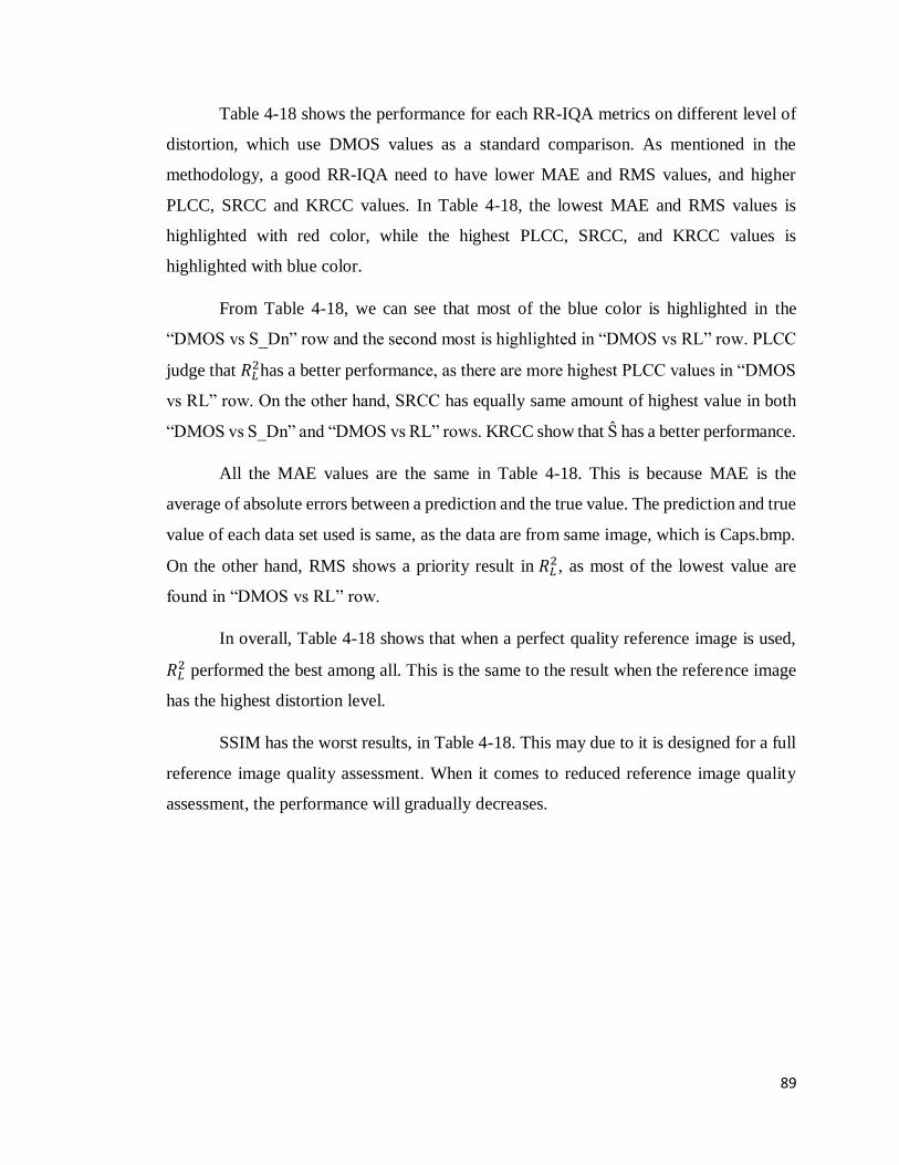
89
Table 4-18 shows the performance for each RR-IQA metrics on different level of
distortion, which use DMOS values as a standard comparison. As mentioned in the
methodology, a good RR-IQA need to have lower MAE and RMS values, and higher
PLCC, SRCC and KRCC values. In Table 4-18, the lowest MAE and RMS values is
highlighted with red color, while the highest PLCC, SRCC, and KRCC values is
highlighted with blue color.
From Table 4-18, we can see that most of the blue color is highlighted in the
“DMOS vs S_Dn” row and the second most is highlighted in “DMOS vs RL” row. PLCC
judge that 𝑅𝐿2has a better performance, as there are more highest PLCC values in “DMOS
vs RL” row. On the other hand, SRCC has equally same amount of highest value in both
“DMOS vs S_Dn” and “DMOS vs RL” rows. KRCC show that S has a better performance.
All the MAE values are the same in Table 4-18. This is because MAE is the
average of absolute errors between a prediction and the true value. The prediction and true
value of each data set used is same, as the data are from same image, which is Caps.bmp.
On the other hand, RMS shows a priority result in 𝑅𝐿2, as most of the lowest value are
found in “DMOS vs RL” row.
In overall, Table 4-18 shows that when a perfect quality reference image is used,
𝑅𝐿2 performed the best among all. This is the same to the result when the reference image
has the highest distortion level.
SSIM has the worst results, in Table 4-18. This may due to it is designed for a full
reference image quality assessment. When it comes to reduced reference image quality
assessment, the performance will gradually decreases.

90
Figure 4-9: Graph plotted by IQM results versus bit rate of imperfect reference
image. It is to show the relationship of each metrics, with different bit rate value of
Gaussian Noise distorted value, and different level of distortion for JPEG2000
distorted reference image.
00.20.40.60.8
11.2
JPEG vs G. Noise
(bit rate = 0)
SSIM S_Dn Rs RL
00.20.40.60.8
11.2
JPEG vs G. Noise
(bit rate = 0.015625)
SSIM S_Dn Rs RL
0
0.2
0.4
0.6
0.8
1
1.2
JPEG vs G. Noise
(bit rate = 0.03125)
SSIM S_Dn Rs RL
0
0.2
0.4
0.6
0.8
1
1.2
JPEG vs G. Noise
(bit rate = 0.0625)
SSIM S_Dn Rs RL
00.20.40.60.8
11.2
JPEG vs G. Noise
(bit rate = 0.125)
SSIM S_Dn Rs RL
00.20.40.60.8
11.2
JPEG vs G. Noise
(bit rate = 1)
SSIM S_Dn Rs RL

91
In Figure 4-9, it shows the graph plotted for each metrics with different bit rate
value of distortion. The graph is used to show the performance of each metrics when the
bit rate value of Gaussian noise distorted image is increasing, and the JPEG2000 distorted
reference image has different distortion value, which is in x-axis of the graph. The flatter
the pattern of the graph, indicates a better consistency of the IQM tested.
From Figure 4-9, 𝑅𝑠2 has a better consistency as compared to other metrics, for all
the Gaussian noise distorted image. 𝑅𝐿2 shows a second best performance in this
assessment, especially when the Gaussian noise distorted image has higher bit rate. Here,
we can say that 𝑅𝐿2 provide a consistent assessment to JPEG2000 reduced reference image
when compared with Gaussian noise distorted image, which is in higher bit rate.
In overall, S shows a better accuracy whereas 𝑅𝐿2 shows a better consistency here,
as compared to the other metrics included, when the reference image has JPEG2000
distortion is compared to Gaussian Noise distorted image.
4-3-2 Fast Fading distorted image as compressed image
Table 4-19 (a) used a perfect quality image as the reference while (b), (c), (d), (e) and (f)
used a JPEG2000 distorted image as the reference image. The bit rate of distortion
increases from (b) to (f). The result value more than one is converted to one in this table.
This is because the highest value qualified is one. From Table 4-19, we can see that the
SSIM, 𝑅𝐹2, PSNR, and 𝑅𝐿
2 value is changing gradually from (a) to (f).
SSIM is a metric designed for full reference image quality assessment. The value
of SSIM changes randomly from (a) to (f) for each of the different bit rate for JPEG2000
reference image. This indicates that SSIM value is less effective when the reference image
used has no perfect quality, and the bit rate of distortion increases.

92
The PSNR value changes inconsistently in value from (a) to (f). This is because
PSNR is calculated by the mean square error of the two images involved. When the
reference image is distorted, it could hardly give an accurate image quality assessment
result.
Table 4-19: Results of each metrics applied on a Fast Fading compressed image,
caps.bmp, with different level of bit rate. The imperfect reference image used is with
JPEG2000 distortion. (a)Perfect quality image as reference. (b)JPEG2000 distorted
image with bit rate 0.050378 as reference. (c)JPEG2000 distorted image with bit rate
0.098741 as reference. (d) JPEG2000 distorted image with bit rate 0.19944 as
reference. (e)JPEG2000 distorted image with bit rate 0.40137 as reference.
(f)JPEG2000 distorted image with bit rate 0.60354 as reference.
Bit rate of JPEG2000 =0
Bit Rate SSIM PSNR S_Dn Rs L RL DMOS
0 1 65535 0.954867 1 1 1 100
15.5 0.7297412 25.41353 0.784455 0.936684 0.787033 1 69.00739
18.9 0.796929 26.59974 0.803897 0.952255 0.804078 1 60.05539
20.3 0.9101077 29.91208 0.88453 0.97799 0.78493 1 50.70893
23.7 0.9820205 36.04244 0.945002 0.994681 1.085079 0.91669 34.45273
25.1 0.9670201 34.6269 0.90351 0.99263 1.084411 0.915362 42.48964
(a)
Bit rate of JPEG2000 =0.050378
Bit Rate SSIM PSNR S_Dn Rs L RL DMOS
0 0.8318948 28.98727 0.81952 0.972697 0.962246 1 100
15.5 0.8362347 27.62309 0.98968 0.960493 1.144767 0.83903 69.00739
18.9 0.8670001 28.88964 0.987747 0.970773 1.162034 0.835408 60.05539
20.3 0.8905735 32.39134 0.965517 0.987114 1.142637 0.863891 50.70893
23.7 0.8457546 29.93694 0.820673 0.977848 0.98235 0.995418 34.45273
25.1 0.8291761 29.47077 0.835784 0.975432 0.982468 0.992839 42.48964
(b)
Bit rate of JPEG2000 =0.098741
Bit Rate SSIM PSNR S_Dn Rs L RL DMOS
0 0.8891991 30.8188 0.867124 0.982177 0.977525 1 100
15.5 0.7876242 26.63278 0.981579 0.951021 1.058354 0.898585 69.00739

93
18.9 0.8566593 28.18228 0.983255 0.96605 1.075568 0.898177 60.05539
20.3 0.9179592 32.30432 0.979286 0.986987 1.056231 0.934443 50.70893
23.7 0.9033107 32.24996 0.874471 0.987057 0.997567 0.989465 34.45273
25.1 0.8861417 31.45271 0.882614 0.984507 0.997684 0.986792 42.48964
(c)
Bit rate of JPEG2000 =0.19944
Bit Rate SSIM PSNR S_Dn Rs L RL DMOS
0 0.9298985 33.27789 0.849209 0.989921 0.991715 0.998191 100
15.5 0.7657489 26.05069 0.903934 0.944543 0.978103 0.965689 69.00739
18.9 0.8342767 27.395 0.919891 0.959686 0.995267 0.964249 60.05539
20.3 0.9133778 31.05171 0.969349 0.982808 0.975986 1 50.70893
23.7 0.9394356 34.36608 0.893781 0.992077 1.011699 0.980606 34.45273
25.1 0.9226294 33.27805 0.881777 0.989857 1.011816 0.978298 42.48964
(d)
Bit rate of JPEG2000 =0.40137
Bit Rate SSIM PSNR S_Dn Rs L RL DMOS
0 0.9644935 36.69453 0.917166 0.995423 1.015466 0.980262 100
15.5 0.7486144 25.67798 0.790531 0.940033 0.843777 1 69.00739
18.9 0.8149839 26.92409 0.811567 0.955404 0.860858 1 60.05539
20.3 0.9148344 30.42855 0.90375 0.980319 0.84167 1 50.70893
23.7 0.9623294 35.46127 0.953522 0.993873 1.14244 0.869956 34.45273
25.1 0.9467813 34.17635 0.911751 0.991782 1.141771 0.868634 42.48964
(e)
Bit rate of JPEG2000 =0.60354
Bit Rate SSIM PSNR S_Dn Rs L RL DMOS
0 0.9776377 39.26188 0.935513 0.997469 1.022654 0.975373 100
15.5 0.7402399 25.52102 0.784784 0.938015 0.80313 1 69.00739
18.9 0.8072687 26.73348 0.804541 0.953544 0.820186 1 60.05539
20.3 0.9141381 30.12626 0.892236 0.978971 0.801027 1 50.70893
23.7 0.9716736 35.9608 0.960453 0.994556 1.101352 0.903033 34.45273
25.1 0.9564238 34.57554 0.914857 0.99252 1.100684 0.90173 42.48964
(f)
Besides, the value of 𝑅𝑠2 also show a changes from Table 4-19 (a) to (f). However,
the changes of the value is averagely small. This shows that 𝑅𝑠2 is suitable for reduced

94
reference image quality assessment. On the other hand, the values of 𝑅𝐿2 have little
changes from Table 4-19 (a) to (f). However, from (f), we can see that 𝑅𝐿2 provided a better
result than 𝑅𝑠2 in certain level of fast fading distortion in distorted image. The distortion is
non-noticeable because the bit rate of distorted image is relatively small, which indicates
that the distorted image is considered high quality. Therefore, the result value is close to
1 although the bit rate is the highest here.
The S value calculated from 𝐷𝑛 value changes randomly in overall, as we can see
from Table 4-19 (a) to (f). However, the S value is less than the value of 𝑅𝑠2 and 𝑅𝐹
2 in
general. This indicates that the estimated SSIM, S is less accurate and less effective for
this assessment.
Table 4-20 shows the performance for each RR-IQA metrics on different level of
distortion, which use DMOS values as a standard comparison. As mentioned in the
methodology, a good RR-IQA need to have lower MAE and RMS values, and higher
PLCC, SRCC and KRCC values. In Table 4-6, the lowest MAE and RMS values is
highlighted with red color, while the highest PLCC, SRCC, and KRCC values is
highlighted with blue color.
From Table 4-20, we can see that most of the blue color is highlighted in the
“DMOS vs Rs” row and the second most is highlighted in “DMOS vs RL” row. PLCC
judge that 𝑅𝐿2 has a better performance, as there are more highest PLCC values in “DMOS
vs RL” row. On the other hand, SRCC judge that both the 𝑅𝑠2 and 𝑅𝐿
2 has equally good
performance in this assessment. KRCC show that 𝑅𝑠2has a better performance.
All the MAE values are the same in Table 4-20. This is because MAE is the
average of absolute errors between a prediction and the true value. The prediction and true
value of each data set used is same, as the data are from same image, which is Caps.bmp.
On the other hand, RMS shows a priority result in 𝑅𝑠2, as most of the lowest value are
found in “DMOS vs Rs” row.

95
Table 4-20: Results of each metrics used to judge the performance of RR-IQA
metrics used.
Bit Rate PLCC MAE RMSE SRCC KRCC
DMOS vs
SSIM
0 -0.07063 59.45235 62.31471 -0.14286 -0.33333
0.050378 -0.26689 59.45235 62.35888 -0.14286 -0.2
0.098741 -0.28265 59.45235 62.33903 -0.42857 -0.33333
0.19944 -0.19749 59.45235 62.3291 -0.42857 -0.46667
0.40137 -0.13031 59.45235 62.32119 -0.14286 -0.33333
0.60354 -0.11369 59.45235 62.31865 -0.14286 -0.33333
DMOS vs
S_Dn
0 0.001619 59.45235 62.32935 -0.14286 -0.33333
0.050378 0.014578 59.45235 62.30667 0.142857 0.333333
0.098741 -0.0385 59.45235 62.28434 0.085714 0.2
0.19944 -0.45749 59.45235 62.31293 -0.14286 -0.2
0.40137 -0.26066 59.45235 62.33278 -0.42857 -0.46667
0.60354 -0.16911 59.45235 62.33065 -0.42857 -0.46667
DMOs vs
Rs
0 -0.061 59.45235 62.23934 -0.14286 -0.33333
0.050378 -0.40993 59.45235 62.24151 -0.65714 -0.46667
0.098741 -0.29844 59.45235 62.23965 -0.77143 -0.6
0.19944 -0.19219 59.45235 62.2393 -0.42857 -0.46667
0.40137 -0.11866 59.45235 62.2393 -0.14286 -0.33333
0.60354 -0.09602 59.45235 62.23945 -0.14286 -0.33333
DMOS vs
RL
0 0.695078 59.45235 62.23291 0.777542 0.602464
0.050378 -0.02187 59.45235 62.29076 -0.08571 -0.2
0.098741 0.005519 59.45235 62.26176 -0.08571 -0.2
0.19944 0.240052 59.45235 62.23256 -0.08571 -0.06667
0.40137 0.612963 59.45235 62.24754 0.5161 0.298142
0.60354 0.549827 59.45235 62.24218 0.5161 0.298142
In overall, Table 4-20 shows that when a perfect quality reference image is used,
𝑅𝐿2 performed the best among all. This is the same to the result when the reference image
has the highest distortion level.
SSIM has the worst results, in Table 4-20. This may due to it is designed for a full
reference image quality assessment. When it comes to reduced reference image quality
assessment, the performance will gradually decreases.

96
Figure 4-10: Graph plotted by IQM results versus bit rate of imperfect reference
image. It is to show the relationship of each metrics, with different bit rate value of
fast fading distorted value, and different level of distortion for JPEG2000 distorted
reference image.
00.20.40.60.8
11.2
JPEG2k vs F. Fading
(bit rate = 0)
SSIM S_Dn Rs RL
00.20.40.60.8
11.2
JPEG2k vs F. Fading
(bit rate = 15.5)
SSIM S_Dn Rs RL
00.20.40.60.8
11.2
JPEG2k vs F. Fading
(bit rate = 18.9)
SSIM S_Dn Rs RL
0.750.8
0.850.9
0.951
1.05
JPEG2k vs F. Fading
(bit rate = 20.3)
SSIM S_Dn Rs RL
00.20.40.60.8
11.2
JPEG2k vs F. Fading
(bit rate = 23.7)
SSIM S_Dn Rs RL
0.70.75
0.80.85
0.90.95
11.05
JPEG2k vs F. Fading
(bit rate = 25.1)
SSIM S_Dn Rs RL

97
In Figure 4-10, it shows the graph plotted for each metrics with different bit rate
value of distortion. The graph is used to show the performance of each metrics when the
bit rate value of fast fading distorted image is increasing, and the JPEG2000 distorted
reference image has different distortion value, which is in x-axis of the graph. The flatter
the pattern of the graph, indicates a better consistency of the IQM tested.
From Figure 4-10, 𝑅𝑠2 has a better consistency as compared to other metrics, for
all the fast fading distorted image. 𝑅𝐿2 only shows a better performance, when fast fading
has zero level of distortion. Here, we can say that 𝑅𝑠2 provide a consistent assessment to
JPEG2000 reduced reference image as tested with fast fading distorted image.
In overall, the performance of the 𝑅𝑠2 are the best as compared to the other metrics
included, when the reference image has JPEG2000 distortion is compared to fast fading
distorted image. This is because 𝑅𝑠2 shows a better accuracy and consistency here.
4-3-3 JPEG distorted image as compressed image
Table 4-21 (a) used a perfect quality image as the reference while (b), (c), (d), (e) and (f)
used a JPEG distorted image as the reference image. The bit rate of distortion increases
from (b) to (f). The result value more than one is converted to one in this table. This is
because the highest value qualified is one. From Table 4-21, we can see that the SSIM,
𝑅𝐹2, PSNR, and 𝑅𝐿
2 value is changing gradually from (a) to (f).
SSIM is a metric designed for full reference image quality assessment. The value
of SSIM changes randomly from (a) to (f) for each of the different bit rate for JPEG2000
reference image. This indicates that SSIM value is less effective when the reference image
used has no perfect quality, and the bit rate of distortion increases.
The PSNR value also changes inconsistently in value from (a) to (f). This is
because PSNR is calculated by the mean square error of the two images involved. When
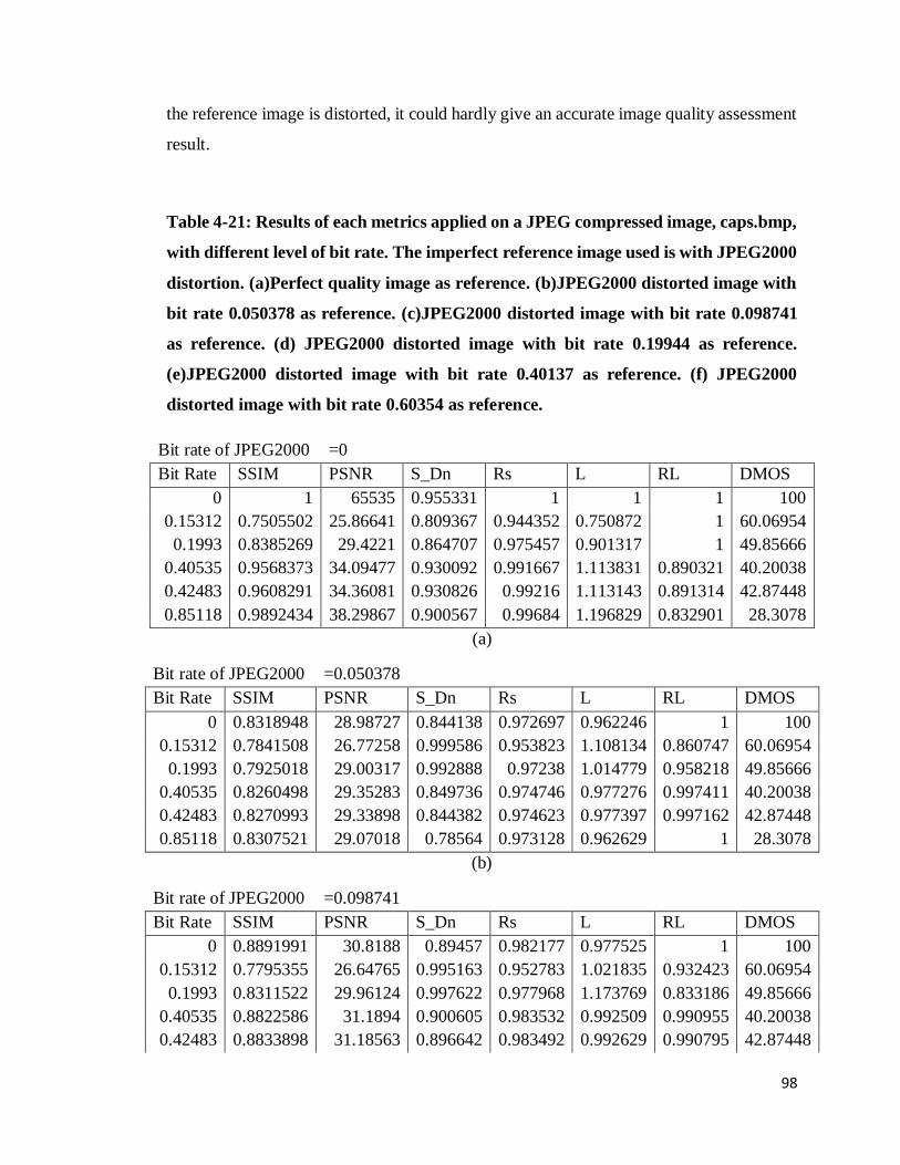
98
the reference image is distorted, it could hardly give an accurate image quality assessment
result.
Table 4-21: Results of each metrics applied on a JPEG compressed image, caps.bmp,
with different level of bit rate. The imperfect reference image used is with JPEG2000
distortion. (a)Perfect quality image as reference. (b)JPEG2000 distorted image with
bit rate 0.050378 as reference. (c)JPEG2000 distorted image with bit rate 0.098741
as reference. (d) JPEG2000 distorted image with bit rate 0.19944 as reference.
(e)JPEG2000 distorted image with bit rate 0.40137 as reference. (f) JPEG2000
distorted image with bit rate 0.60354 as reference.
Bit rate of JPEG2000 =0
Bit Rate SSIM PSNR S_Dn Rs L RL DMOS
0 1 65535 0.955331 1 1 1 100
0.15312 0.7505502 25.86641 0.809367 0.944352 0.750872 1 60.06954
0.1993 0.8385269 29.4221 0.864707 0.975457 0.901317 1 49.85666
0.40535 0.9568373 34.09477 0.930092 0.991667 1.113831 0.890321 40.20038
0.42483 0.9608291 34.36081 0.930826 0.99216 1.113143 0.891314 42.87448
0.85118 0.9892434 38.29867 0.900567 0.99684 1.196829 0.832901 28.3078
(a)
Bit rate of JPEG2000 =0.050378
Bit Rate SSIM PSNR S_Dn Rs L RL DMOS
0 0.8318948 28.98727 0.844138 0.972697 0.962246 1 100
0.15312 0.7841508 26.77258 0.999586 0.953823 1.108134 0.860747 60.06954
0.1993 0.7925018 29.00317 0.992888 0.97238 1.014779 0.958218 49.85666
0.40535 0.8260498 29.35283 0.849736 0.974746 0.977276 0.997411 40.20038
0.42483 0.8270993 29.33898 0.844382 0.974623 0.977397 0.997162 42.87448
0.85118 0.8307521 29.07018 0.78564 0.973128 0.962629 1 28.3078
(b)
Bit rate of JPEG2000 =0.098741
Bit Rate SSIM PSNR S_Dn Rs L RL DMOS
0 0.8891991 30.8188 0.89457 0.982177 0.977525 1 100
0.15312 0.7795355 26.64765 0.995163 0.952783 1.021835 0.932423 60.06954
0.1993 0.8311522 29.96124 0.997622 0.977968 1.173769 0.833186 49.85666
0.40535 0.8822586 31.1894 0.900605 0.983532 0.992509 0.990955 40.20038
0.42483 0.8833898 31.18563 0.896642 0.983492 0.992629 0.990795 42.87448

99
0.85118 0.8878785 30.90933 0.852637 0.982489 0.977907 1 28.3078
(c)
Bit rate of JPEG2000 =0.19944
Bit Rate SSIM PSNR S_Dn Rs L RL DMOS
0 0.9298985 33.27789 0.895235 0.989921 0.991715 0.998191 100
0.15312 0.7728114 26.3504 0.949794 0.949738 0.94169 1 60.06954
0.1993 0.8430102 30.02987 0.975741 0.978432 1.093184 0.895029 49.85666
0.40535 0.9191501 32.89558 0.918263 0.988922 1.006655 0.982384 40.20038
0.42483 0.9206346 32.94235 0.914034 0.989025 1.006776 0.982369 42.87448
0.85118 0.9278998 33.19251 0.86839 0.989687 0.992096 0.997572 28.3078
(d)
Bit rate of JPEG2000 =0.40137
Bit Rate SSIM PSNR S_Dn Rs L RL DMOS
0 0.9644935 36.69453 0.910754 0.995423 1.015466 0.980262 100
0.15312 0.7644716 26.09408 0.800669 0.946952 0.807542 1 60.06954
0.1993 0.8448925 29.74813 0.861601 0.977111 0.958298 1 49.85666
0.40535 0.9452103 33.85251 0.946376 0.991145 1.171252 0.846227 40.20038
0.42483 0.9478214 34.03657 0.945573 0.991505 1.170563 0.847033 42.87448
0.85118 0.9614563 35.73002 0.909715 0.994267 1.015846 0.978758 28.3078
(e)
Bit rate of JPEG2000 =0.60354
Bit Rate SSIM PSNR S_Dn Rs L RL DMOS
0 0.9776377 39.26188 0.929541 0.997469 1.022654 0.975373 100
0.15312 0.7594967 25.96464 0.788272 0.945468 0.766948 1 60.06954
0.1993 0.8433876 29.57165 0.847119 0.976222 0.917482 1 49.85666
0.40535 0.953084 34.08496 0.95392 0.991625 1.13012 0.877451 40.20038
0.42483 0.9562472 34.3125 0.954712 0.992047 1.129432 0.878359 42.87448
0.85118 0.973876 37.0217 0.928547 0.995749 1.023032 0.973331 28.3078
(f)
Besides, the value of 𝑅𝑠2 also show a gradual changes from Table 4-21 (a) to (f).
However, the changes of the value is averagely small. This shows that 𝑅𝑠2 is suitable for
reduced reference image quality assessment. On the other hand, the values of 𝑅𝐿2 changes
accordingly with the pattern of other metrics from Table 4-21 (a) to (f). From (f), we can
see that 𝑅𝑠2 provided a better result than 𝑅𝐿
2 in overall. The distortion is non-noticeable

100
because the bit rate of distorted image is relatively small, which indicates that the distorted
image is considered high quality. Therefore, the result value is close to 1 although the bit
rate is the highest here.
The S value calculated from 𝐷𝑛 value changes accordingly in overall, as we can
see from Table 4-21 (a) to (f). However, the S value is less than the value of 𝑅𝑠2 and 𝑅𝐹
2 in
general. This indicates that the estimated SSIM, S is less accurate and less effective for
this assessment.
Table 4-22: Results of each metrics used to judge the performance of RR-IQA
metrics used.
Bit Rate PLCC MAE RMSE SRCC KRCC
DMOS vs
SSIM
0 0.018983 53.55148 57.39575 -0.08571 -0.2
0.050378 -0.00284 53.55148 57.48865 -0.08571 -0.2
0.098741 -0.05578 53.55148 57.44965 -0.08571 -0.2
0.19944 -0.0509 53.55148 57.42549 -0.08571 -0.2
0.40137 -0.03406 53.55148 57.40777 -0.08571 -0.2
0.60354 -0.02458 53.55148 57.40215 -0.08571 -0.2
DMOS vs
S_Dn
0 0.203077 53.55148 57.40849 0.085714 0.066667
0.050378 0.167842 53.55148 57.41847 0.371429 0.333333
0.098741 0.164863 53.55148 57.38651 0.314286 0.2
0.19944 0.047498 53.55148 57.39182 0.314286 0.2
0.40137 -0.19336 53.55148 57.41887 -0.37143 -0.33333
0.60354 -0.13983 53.55148 57.41419 -0.31429 -0.2
DMOs vs
Rs
0 0.001028 53.55148 57.33454 -0.08571 -0.2
0.050378 -0.1779 53.55148 57.34716 -0.65714 -0.46667
0.098741 -0.14271 53.55148 57.34099 -0.65714 -0.46667
0.19944 -0.09557 53.55148 57.33736 -0.08571 -0.2
0.40137 -0.05117 53.55148 57.33552 -0.08571 -0.2
0.60354 -0.0325 53.55148 57.33508 -0.08571 -0.2
DMOS vs
RL
0 0.742814 53.55148 57.35841 0.941124 0.894427
0.050378 -0.09909 53.55148 57.34986 -0.28989 -0.41404
0.098741 0.047575 53.55148 57.35683 -0.23191 -0.27603
0.19944 0.1556 53.55148 57.33914 0.371429 0.066667
0.40137 0.354058 53.55148 57.36292 0.637748 0.414039
0.60354 0.341357 53.55148 57.35736 0.637748 0.414039

101
Table 4-22 shows the performance for each RR-IQA metrics on different level of
distortion, which use DMOS values as a standard comparison. As mentioned in the
methodology, a good RR-IQA need to have lower MAE and RMS values, and higher
PLCC, SRCC and KRCC values. In Table 4-22, the lowest MAE and RMS values is
highlighted with red color, while the highest PLCC, SRCC, and KRCC values is
highlighted with blue color.
From Table 4-22, we can see that most of the blue color is highlighted in the
“DMOS vs RL” row and the second most is highlighted in “DMOS vs Rs” row. In such,
PLCC, SRCC, and KRCC judge that 𝑅𝐿2 has a better performance, as there are more
highest PLCC, SRCC, and KRCC values in “DMOS vs RL” row.
All the MAE values are the same in Table 4-22. This is because MAE is the
average of absolute errors between a prediction and the true value. The prediction and true
value of each data set used is same, as the data are from same image, which is Caps.bmp.
On the other hand, RMS shows a priority result in 𝑅𝑠2, as all of the lowest value are found
in “DMOS vs RL” row.
In overall, Table 4-22 shows that when a perfect quality reference image is used,
𝑅𝐿2 performed the best among all. This is the same to the result when the reference image
has the highest distortion level.
SSIM has the worst results, in Table 4-22. This may due to it is designed for a full
reference image quality assessment. When it comes to reduced reference image quality
assessment, the performance will gradually decreases.
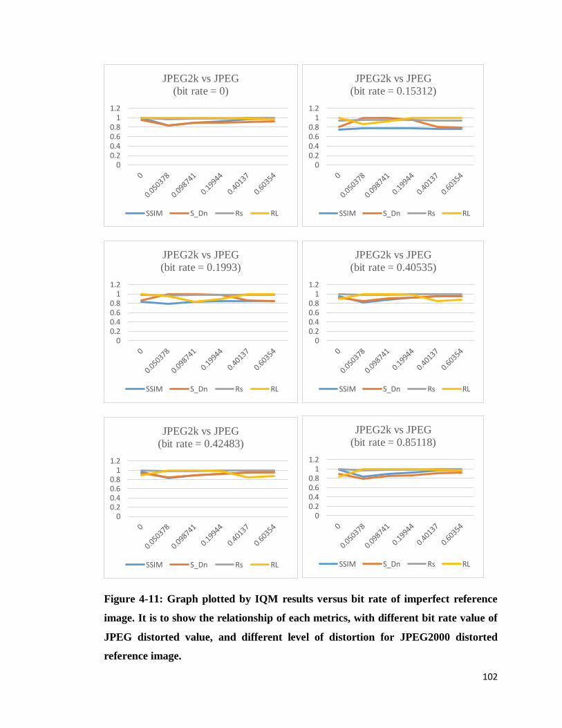
102
Figure 4-11: Graph plotted by IQM results versus bit rate of imperfect reference
image. It is to show the relationship of each metrics, with different bit rate value of
JPEG distorted value, and different level of distortion for JPEG2000 distorted
reference image.
00.20.40.60.8
11.2
JPEG2k vs JPEG
(bit rate = 0)
SSIM S_Dn Rs RL
00.20.40.60.8
11.2
JPEG2k vs JPEG
(bit rate = 0.15312)
SSIM S_Dn Rs RL
00.20.40.60.8
11.2
JPEG2k vs JPEG
(bit rate = 0.1993)
SSIM S_Dn Rs RL
00.20.40.60.8
11.2
JPEG2k vs JPEG
(bit rate = 0.40535)
SSIM S_Dn Rs RL
00.20.40.60.8
11.2
JPEG2k vs JPEG
(bit rate = 0.42483)
SSIM S_Dn Rs RL
00.20.40.60.8
11.2
JPEG2k vs JPEG
(bit rate = 0.85118)
SSIM S_Dn Rs RL

103
In Figure 4-11, it shows the graph plotted for each metrics with different bit rate
value of distortion. The graph is used to show the performance of each metrics when the
bit rate value of JPEG distorted image is increasing, and the JPEG2000 distorted reference
image has different distortion value, which is in x-axis of the graph. The flatter the pattern
of the graph, indicates a better consistency of the IQM tested.
From Figure 4-11, 𝑅𝑠2 has a better consistency as compared to other metrics, for
all distortion level of the JPEG distorted image. 𝑅𝐿2 only shows a better performance when
JPEG distortion level is zero. Here, we can say that 𝑅𝑠2 provide a consistent assessment to
JPEG2000 reduced reference image when compared with JPEG distorted image.
In overall, 𝑅𝐿2 shows a better accuracy and 𝑅𝑠
2 gives a better consistency here, as
compared to the other metrics included, when the reference image has JPEG2000
distortion is compared to JPEG distorted image.
4-3-4 Gaussian Blur distorted image as compressed image
Table 4-23 (a) used a perfect quality image as the reference while (b), (c), (d), (e) and (f)
used a JPEG2000 distorted image as the reference image. The bit rate of distortion
increases from (b) to (f). The result value more than one is converted to one in this table.
This is because the highest value qualified is one. From Table 4-23, we can see that the
SSIM, 𝑅𝐹2, PSNR, and 𝑅𝐿
2 value changes gradually from (a) to (f).
SSIM is a metric designed for full reference image quality assessment. The value
of SSIM show an inconsistent changes when Gaussian blur distorted image has higher
distortion level from (a) to (f). This indicates that SSIM value is less effective when the
reference image used has no perfect quality, and the bit rate of distortion increases.
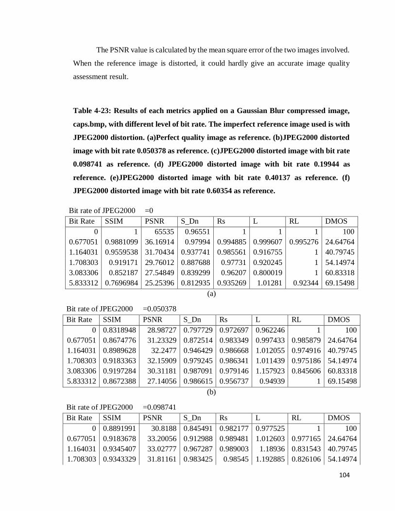
104
The PSNR value is calculated by the mean square error of the two images involved.
When the reference image is distorted, it could hardly give an accurate image quality
assessment result.
Table 4-23: Results of each metrics applied on a Gaussian Blur compressed image,
caps.bmp, with different level of bit rate. The imperfect reference image used is with
JPEG2000 distortion. (a)Perfect quality image as reference. (b)JPEG2000 distorted
image with bit rate 0.050378 as reference. (c)JPEG2000 distorted image with bit rate
0.098741 as reference. (d) JPEG2000 distorted image with bit rate 0.19944 as
reference. (e)JPEG2000 distorted image with bit rate 0.40137 as reference. (f)
JPEG2000 distorted image with bit rate 0.60354 as reference.
Bit rate of JPEG2000 =0
Bit Rate SSIM PSNR S_Dn Rs L RL DMOS
0 1 65535 0.96551 1 1 1 100
0.677051 0.9881099 36.16914 0.97994 0.994885 0.999607 0.995276 24.64764
1.164031 0.9559538 31.70434 0.937741 0.985561 0.916755 1 40.79745
1.708303 0.919171 29.76012 0.887688 0.97731 0.920245 1 54.14974
3.083306 0.852187 27.54849 0.839299 0.96207 0.800019 1 60.83318
5.833312 0.7696984 25.25396 0.812935 0.935269 1.01281 0.92344 69.15498
(a)
Bit rate of JPEG2000 =0.050378
Bit Rate SSIM PSNR S_Dn Rs L RL DMOS
0 0.8318948 28.98727 0.797729 0.972697 0.962246 1 100
0.677051 0.8674776 31.23329 0.872514 0.983349 0.997433 0.985879 24.64764
1.164031 0.8989628 32.2477 0.946429 0.986668 1.012055 0.974916 40.79745
1.708303 0.9183363 32.15909 0.979245 0.986341 1.011439 0.975186 54.14974
3.083306 0.9197284 30.31181 0.987091 0.979146 1.157923 0.845606 60.83318
5.833312 0.8672388 27.14056 0.986615 0.956737 0.94939 1 69.15498
(b)
Bit rate of JPEG2000 =0.098741
Bit Rate SSIM PSNR S_Dn Rs L RL DMOS
0 0.8891991 30.8188 0.845491 0.982177 0.977525 1 100
0.677051 0.9183678 33.20056 0.912988 0.989481 1.012603 0.977165 24.64764
1.164031 0.9345407 33.02777 0.967287 0.989003 1.18936 0.831543 40.79745
1.708303 0.9343329 31.81161 0.983425 0.98545 1.192885 0.826106 54.14974

105
3.083306 0.9031943 29.2993 0.979936 0.974056 1.071469 0.909085 60.83318
5.833312 0.8295402 26.35671 0.973648 0.948726 0.96471 0.983431 69.15498
(c)
Bit rate of JPEG2000 =0.19944
Bit Rate SSIM PSNR S_Dn Rs L RL DMOS
0 0.9298985 33.27789 0.846149 0.989921 0.991715 0.998191 100
0.677051 0.9463335 34.63151 0.938962 0.992504 1.192159 0.832527 24.64764
1.164031 0.9440675 32.62334 0.972405 0.988091 1.108729 0.891192 40.79745
1.708303 0.9283536 30.87118 0.95131 0.98215 1.112244 0.883035 54.14974
3.083306 0.8828013 28.44585 0.911358 0.96873 0.99118 0.97735 60.83318
5.833312 0.8071262 25.83444 0.883599 0.942673 0.978937 0.962956 69.15498
(d)
Bit rate of JPEG2000 =0.40137
Bit Rate SSIM PSNR S_Dn Rs L RL DMOS
0 0.9644935 36.69453 0.939593 0.995423 1.015466 0.980262 100
0.677051 0.9681861 35.52851 0.973787 0.993978 1.056791 0.940562 24.64764
1.164031 0.9514637 32.14243 0.947352 0.986833 0.973768 1 40.79745
1.708303 0.9252225 30.23945 0.899947 0.979535 0.977265 1 54.14974
3.083306 0.8683226 27.92243 0.853973 0.964981 0.85679 1 60.83318
5.833312 0.7890685 25.49545 0.824365 0.93842 1.00275 0.935846 69.15498
(e)
Bit rate of JPEG2000 =0.60354
Bit Rate SSIM PSNR S_Dn Rs L RL DMOS
0 0.9776377 39.26188 0.952836 0.997469 1.022654 0.975373 100
0.677051 0.9759931 35.71695 0.97503 0.994272 1.015829 0.978779 24.64764
1.164031 0.9535834 31.86576 0.940036 0.986025 0.932929 1 40.79745
1.708303 0.923177 29.95207 0.892432 0.978209 0.936421 1 54.14974
3.083306 0.8617872 27.69965 0.8484 0.963244 0.816124 1 60.83318
5.833312 0.7805744 25.35055 0.821806 0.936494 1.009956 0.927262 69.15498
(f)
Besides, the value of 𝑅𝑠2 also show a changes from Table 4-23(a) to (f). However,
the changes of the value is averagely small. This shows that 𝑅𝑠2 is suitable for reduced
reference image quality assessment. On the other hand, the values of 𝑅𝐿2 also changes by
little difference from Table 4-23 (a) to (f). However, from (f), we can see that 𝑅𝐿2 provided

106
a better result than 𝑅𝑠2 at the Gaussian blur distortion bit rate of 1.164031, 1.708303, and
3.083306. The distortion is non-noticeable because the bit rate of distorted image is
relatively small, which indicates that the distorted image is considered high quality.
Therefore, the result value is close to 1 although the bit rate is the highest here.
The S value calculated from 𝐷𝑛 value changes accordingly in overall, as we can
see from Table 4-23 (a) to (f). However, the S value is less than the value of 𝑅𝑠2 and 𝑅𝐹
2 in
general. This indicates that the estimated SSIM, S is less accurate and less effective for
this assessment.
Table 4-24 shows the performance for each RR-IQA metrics on different level of
distortion, which use DMOS values as a standard comparison. As mentioned in the
methodology, a good RR-IQA need to have lower MAE and RMS values, and higher
PLCC, SRCC and KRCC values. In Table 4-6, the lowest MAE and RMS values is
highlighted with red color, while the highest PLCC, SRCC, and KRCC values is
highlighted with blue color.
From Table 4-24, we can see that most of the blue color is highlighted in the
“DMOS vs S_Dn” row and the second most is highlighted in “DMOS vs Rs” and “DMOS
vs RL” rows. PLCC judge that both S and 𝑅𝐿2 has a better performance, as there are more
highest PLCC values in “DMOs vs S_Dn” and “DMOS vs RL” row. On the other hand,
SRCC and KRCC show that S has a better performance.
All the MAE values are the same in Table 4-24. This is because MAE is the
average of absolute errors between a prediction and the true value. The prediction and true
value of each data set used is same, as the data are from same image, which is Caps.bmp.
On the other hand, RMS shows a priority result in 𝑅𝑠2 and 𝑅𝐿
2, as most of the lowest value
are found in “ DMOS vs Rs” and “DMOS vs RL” rows.

107
Table 4-24: Results of each metrics used to judge the performance of RR-IQA
metrics used.
Bit Rate PLCC MAE RMSE SRCC KRCC
DMOS vs
SSIM
0 -0.12137 58.26383 61.98908 -0.14286 -0.33333
0.050378 -0.47546 58.26383 62.01897 -0.42857 -0.2
0.098741 -0.50591 58.26383 62.00394 -0.77143 -0.6
0.19944 -0.32503 58.26383 61.99855 -0.65714 -0.6
0.40137 -0.2092 58.26383 61.99325 -0.42857 -0.46667
0.60354 -0.17466 58.26383 61.99194 -0.14286 -0.33333
DMOS vs
S_Dn
0 -0.18889 58.26383 61.99937 -0.42857 -0.46667
0.050378 -0.33246 58.26383 61.98122 0.085714 0.2
0.098741 -0.45774 58.26383 61.9666 -0.08571 -0.06667
0.19944 -0.86176 58.26383 61.99637 -0.82857 -0.73333
0.40137 -0.34735 58.26383 61.99941 -0.65714 -0.6
0.60354 -0.24996 58.26383 61.99904 -0.42857 -0.46667
DMOs vs
Rs
0 -0.09219 58.26383 61.92903 -0.14286 -0.33333
0.050378 -0.55378 58.26383 61.92893 -0.77143 -0.6
0.098741 -0.3828 58.26383 61.92818 -0.82857 -0.73333
0.19944 -0.24197 58.26383 61.92847 -0.42857 -0.46667
0.40137 -0.15537 58.26383 61.9288 -0.14286 -0.33333
0.60354 -0.12384 58.26383 61.92915 -0.14286 -0.33333
DMOS vs
RL
0 -0.16943 58.26383 61.92027 0.067612 0.086066
0.050378 0.081509 58.26383 61.93795 0.463817 0.276026
0.098741 0.399056 58.26383 61.96805 0.6 0.466667
0.19944 0.89548 58.26383 61.95595 0.885714 0.733333
0.40137 0.121522 58.26383 61.92674 -0.21251 -0.14907
0.60354 -0.30357 58.26383 61.92718 -0.5161 -0.29814
In overall, Table 4-24 shows that when a perfect quality reference image is used,
S performed the best among all. On the other hand, 𝑅𝐿2 performed when the reference
image has the highest distortion level.
SSIM has the worst results, in Table 4-24. This may due to it is designed for a full
reference image quality assessment. When it comes to reduced reference image quality
assessment, the performance will gradually decreases.

108
Figure 4-12: Graph plotted by IQM results versus bit rate of imperfect reference
image. It is to show the relationship of each metrics, with different bit rate value of
Gaussian Blur distorted value, and different level of distortion for JPEG2000
distorted reference image.
00.20.40.60.8
11.2
JPEG2k vs G. Blur
(bit rate =0)
SSIM S_Dn Rs RL
0.750.8
0.850.9
0.951
1.05
JPEG2k vs G. Blur
(bit rate =0.677051)
SSIM S_Dn Rs RL
00.20.40.60.8
11.2
JPEG2k vs G. Blur
(bit rate =1.164031)
SSIM S_Dn Rs RL
00.20.40.60.8
11.2
JPEG2k vs G. Blur
(bit rate =1.708303)
SSIM S_Dn Rs RL
0.750.8
0.850.9
0.951
1.05
JPEG2k vs G. Blur
(bit rate =3.083306)
SSIM S_Dn Rs RL
00.20.40.60.8
11.2
JPEG2k vs G. Blur
(bit rate =5.833312)
SSIM S_Dn Rs RL

109
In Figure 4-12, it shows the graph plotted for each metrics with different bit rate
value of distortion. The graph is used to show the performance of each metrics when the
bit rate value of Fast Fading distorted image is increasing, and the Gaussian Blur distorted
reference image has different distortion value, which is in x-axis of the graph. The flatter
the pattern of the graph, indicates a better consistency of the IQM tested.
From Figure 4-12, 𝑅𝑠2 has a better consistency as compared to other metrics, for
all the Gaussian blur distorted image. 𝑅𝐿2 has the second best performance when Gaussian
blur distortion level is zero and the highest. Here, we can say that 𝑅𝑠2 provide an accurate
assessment to JPEG2000 reduced reference image as compared with Gaussian blur
distorted image.
In overall, S shows a better accuracy whereas 𝑅𝑠2 shows a better consistency here,
as compared to the other metrics included, when the reference image has JPEG2000
distortion is compared to Gaussian blur distorted image.

110
CHAPTER 5
CONCLUSION AND RECOMMENDATIONS
In this paper, a new statistical prior model method, 𝑅𝐿2 reinforced from MULFR model
which is proposed for full reference image quality assessment. The proposed 𝑅𝐿2 is
designed for reduced reference image quality assessment, where there is distortion applied
on the imperfect reference image. This IQM is more reliable in actual applications. A
major characteristic of 𝑅𝐿2 is it flexibility to be used to test on different types of distortions.
To show the effectiveness of 𝑅𝐿2, we tested it on a set of images with different types
of distortions, which are JPEG, JPEG2000, Gaussian Noise, and Gaussian Blur, and
proved that it compares positively with other IQA metrics. 𝑅𝐿2 shows a good performance
when JPEG2000 is used as imperfect reference image. When Gaussian Blur is used on
imperfect reference image, 𝑅𝑠2 and S show a good performance. For JPEG compression
applied on imperfect reference image, 𝑅𝑠2 shows a better consistency and monotonicity.
On the other hand, 𝑅𝐿2 shows a good performance when JPEG2000, JPEG, or Gaussian
Blur is applied on the distorted image. 𝑅𝑠2 shows an overall better performance when Fast
Fading distortion is applied on distorted image. The summary of each IQM performance
can be found from Table 5-1.

111
Table 5.1: Summary of the performance of each IQM.
G. Blur vs JPEG
Monotonicity: 𝑅𝐿2
Accuracy: 𝑅𝑠2
Consistency: 𝑅𝑠2
⟹ Overall: 𝑅𝑠2
JPEG vs G. Noise
Monotonicity: S
Accuracy: S
Consistency: 𝑅𝑠2
⟹ Overall: S
JPEG2K vs G. Noise
Monotonicity: 𝑅𝐿2
Accuracy: 𝑅𝐿2
Consistency: 𝑅𝐿2
⟹ Overall: 𝑅𝐿2
G. Blur vs JPEG2K
Monotonicity: S
Accuracy: S
Consistency: 𝑅𝑠2
⟹ Overall: S
JPEG vs G. Blur
Monotonicity: 𝑅𝑠2
Accuracy: 𝑅𝐿2
Consistency: 𝑅𝑠2
⟹ Overall: 𝑅𝑠2
JPEG2K vs F. Fading
Monotonicity: 𝑅𝑠2
Accuracy: 𝑅𝐿2
Consistency: 𝑅𝑠2
⟹ Overall: 𝑅𝑠2
G. Blur vs G. Noise
Monotonicity: S
Accuracy: S
Consistency: 𝑅𝐿2
⟹ Overall: S
JPEG vs JPEG2K
Monotonicity: 𝑅𝐿2
Accuracy: 𝑅𝐿2
Consistency: 𝑅𝑠2
⟹ Overall: 𝑅𝐿2
JPEG2K vs JPEG
Monotonicity: 𝑅𝐿2
Accuracy: 𝑅𝐿2
Consistency: 𝑅𝑠2
⟹ Overall: 𝑅𝐿2
G. Blur vs F. Fading
Monotonicity: 𝑅𝐿2
Accuracy: 𝑅𝑠2
Consistency: 𝑅𝑠2
⟹ Overall: 𝑅𝑠2
JPEG vs F. Fading
Monotonicity: 𝑅𝑠2
Accuracy: 𝑅𝐿2
Consistency: 𝑅𝑠2
⟹ Overall: 𝑅𝑠2
JPEG2K vs G. Blur
Monotonicity: 𝑅𝐿2
Accuracy: 𝑅𝐿2
Consistency: 𝑅𝑠2
⟹ Overall: 𝑅𝐿2
For the perfect reference image, 𝑅𝐿2 , 𝑅𝑠
2 , SSIM, and PSNR show a very good
performance. They have a good accuracy, consistency, and monotonicity. SSIM is more
suitable for full reference IQA. When the quality of reference image is distorted, we found
that 𝑅𝐿2 performs better than all other IQMs. SSIM could be seriously under measure
image quality for reduced reference image, followed by PSNR, S, and 𝑅𝑠2. This is a major

112
benefit by using 𝑅𝐿2 for IQA, because the perfect quality reference image is hardly obtain
in actual applications, especially for the end-receiver.
There are some limitations found during conduct this study. All the images used
in this study is taken from only one database, which is LIVE database. There are quite a
number of image databases found in this field. By including different image database in a
study, it will improve the IQM results, and make it more reliable. Different level of noise
from different database can provide a more accurate results. Besides, the more accurate
carrying capacity value is found for only three of the distortions, which are Gaussian Blur,
JPEG, and JPEG2000. And so, only these three distortions is used in imperfect reference
image. In order to include more distortion types for imperfect reference image, the
carrying capacity value should be found. This can be done by including and analyzing
more images from different database to get more image constraints for calculating the
carrying capacity value. Besides, by doing so will also improve the existing carrying
capacity value. This will provide a better performance of 𝑅𝐿2.

113
REFERENCES
Abdul, R. and Zhou, W. (2012). Reduced-Reference Image Quality Assessment by
Structural Similarity Estimation. [online] Available at:
https://ece.uwaterloo.ca/~a5rehman/docs/RR_SSIM.pdf [Accessed 8 Jul. 2015].
Archambault, M. (2015). JPEG 2000: The Better Alternative to JPEG That Never Made
it Big. [online] PetaPixel. Available at:
http://petapixel.com/2015/09/12/jpeg-2000-the-better-alternative-to-jpeg-that-never-
made-it-big/ [Accessed 20 Mar. 2016].
Developing for Developers. (2006). How does JPEG actually work?. [online] Available
at: https://blogs.msdn.microsoft.com/devdev/2006/04/12/how-does-jpeg-actually-
work/[Accessed 31 Jan. 2016].
Diwei, Y., Hongwei, L., Huiming, P., Yongluo, S. and Yuantong, S. (2015). Reduced
reference Image Quality Assessment Based on Roberts Derivative Statistic Model of
Natural Image. [online] Available at:
http://www.jofcis.com/publishedpapers/2012_8_5_1837_1844.pdf [Accessed 25 Jul.
2015].
Jinjian, W., Weisi, L., Guangming, S. and Long, X. (n.d.). Reduced-Reference Image
Quality Assessment with Local Binary Structural Pattern. [online] Available at:
http://web.xidian.edu.cn/wjj/files/20140119_184936.pdf [Accessed 18 Mar. 2016].
Min, Z., Wufeng, X. and Xuanqin, M. (2013). Reduced Reference Image Quality
Assessment Based on Statistics of Edge. [online] Available at:
http://ipl.xjtu.edu.cn/ftp/wxue/RR_Min_SPIE2011.pdf [Accessed 8 Jul. 2015].
114
Rajiv, S. and Alan C., B. (2015). Rred Indices: Reduced Reference Entropic
DifferencingFramework For Image Quality Assessment. [online] Available at:
http://live.ece.utexas.edu/publications/2011/rs_icassp_2011.pdf [Accessed 22 Jul.
2015].
Shiqi, W., Xiang, Z., Siwei, M. and Wen, G. (2015). Reduced Reference Image Quality
Assessment Using Entropy of Primitives. [online] Available at:
http://www.jdl.ac.cn/doc/2011/20131021111321509_pid2949423.pdf [Accessed 19
Jul.2015].
Wufeng, X. and Xuanqin, M. (2010). Reduced Reference Image Quality Assessment
Based On Weibull Statistics. [online] Available at:
http://ipl.xjtu.edu.cn/download/wxue/Weibull%20RRIQA2010.pdf [Accessed 8 Jul.
2015].
Zhou, W. and Eero, P. (2005). Reduced-Reference Image Quality Assessment Using A
Wavelet-Domain Natural Image Statistic Model. [online] Available at:
https://ece.uwaterloo.ca/~z70wang/publications/ei05.pdf [Accessed 8 Jul. 2015].