15 AUGUST 2000 2987K A P L A N E T A L .

q 2000 American Meteorological Society

Reduced Space Optimal Interpolation of Historical Marine Sea Level Pressure:1854–1992*

ALEXEY KAPLAN, YOCHANAN KUSHNIR, AND MARK A. CANE

Lamont-Doherty Earth Observatory, Columbia University, Palisades, New York

(Manuscript received 20 April 1999, in final form 8 October 1999)

ABSTRACT

Near-global 48 3 48 gridded analysis of marine sea level pressure (SLP) from the Comprehensive Ocean–Atmosphere Data Set for monthly averages from 1854 to 1992 was produced along with its estimated errorusing a reduced space optimal interpolation method. A novel procedure of covariance adjustment brought theresults of the analysis to the consistency with the a priori assumptions on the signal covariance structure.Comparisons with the National Centers for Environmental Prediction–National Center for Atmospheric Researchglobal atmosphere reanalysis, with the National Center for Atmospheric Research historical analysis of theNorthern Hemisphere SLP, and with the global historical analysis of the U.K. Meteorological Office showencouraging skill of the present product and identifies noninclusion of the land data as its main limitation.Marine SLP pressure proxies are produced for the land stations used in the definitions of the Southern Oscillationand North Atlantic Oscillation (NAO) indices. Surprisingly, they prove to be competitive in quality with theland station records. Global singular value decomposition analysis of the SLP fields versus sea surface temperatureidentified three major patterns of their joint large-scale and long-term variability as ‘‘trend,’’ Pacific decadaloscillation, and NAO.

1. Introduction

The monthly averaged sea level pressure (SLP) canbe viewed as a physical variable that together with seasurface temperature (SST) describes the large-scale be-havior of the ocean–atmosphere interface, the mediumof crucial dynamical importance for the climate and itsvariability. For the presatellite era, the main source ofobservations of this interface are the measurements tak-en on volunteer observing ships. As a result, the ob-servational coverage reflects ship traffic variations, be-ing incomplete at present, quite sparse before 1950, andvirtually nonexistent before the middle of the nineteenthcentury. Compilations of such observations into binnedaverages on a regular latitude–longitude grid with qual-ity control and other statistics have become availableduring the last decade [e.g., Comprehensive Ocean–At-mosphere Data Set (COADS), Woodruff et al. 1987;Global Ocean Surface Temperature Atlas (GOSTA),Bottomley et al. 1990]. We recently developed a methodfor objective optimal analysis of such historical datasets

* Lamont-Doherty Earth Observatory Contribution Number 5982.

Corresponding author address: Dr. Alexey Kaplan, Lamont-Do-herty Earth Observatory, Columbia University, P.O. Box 1000, 61Route 9W, Palisades, NY 10964-8000.E-mail: alexeyk@ldeo.columbia.edu

(Kaplan et al. 1997), and applied it to the MOHSST5version of GOSTA (Parker et al. 1994), producing near-global analysis of monthly SST anomalies for the period1856–1991 (Kaplan et al. 1998, hereafter K98). Thismethod combines a classic approach of least squaresoptimal estimation with the novelty of space reductionand is specifically designed to recover large-scale fea-tures of the observed variable. These features are pre-sumed to be of largest climatic importance, and they areessentially all of the robust signal that can be derivedfrom sparse data. Here we apply a similar approach tothe COADS compilation of SLP observations.

The goal of this work is to produce an optimal anal-ysis of SLP with estimated uncertainty, based solely onmarine observations. Such a product will be useful forthe baseline comparison of more elaborated analyses(those making use of land station data, atmosphericmodels, etc.) that might be produced in the future.

While we were attempting to apply to the COADSSLP data exactly the same technique we used in K98,the differences in the data produced a few alternationsin the procedure. To the large extent, these differencesare caused by the different nature of estimated variables.SLP is known to have larger scales of spatial coherencethan SST has but a much whiter temporal spectrum(Davis 1976). Consequently, the spatial interpolation ofSLP data with main patterns of SLP variability that canbe approximated by eigenvectors of the data samplecovariance matrix [also known as empirical orthogonal

2988 VOLUME 13J O U R N A L O F C L I M A T E

functions (EOFs)] has good prospects, but temporalsmoothing probably will not be useful. As a result, in-stead of the reduced space optimal smoothing techniqueof K98, we use reduced space optimal interpolationhere.

In section 2 we provide a short description of theprocedure, concentrating on the differences between thepresent application and K98. The rest of the paper dealswith the verification of the product we developed. Insection 3 it is compared with the National Centers forEnvironmental Prediction–National Center for Atmo-spheric Research (NCEP–NCAR) global atmosphere re-analysis (Kalnay et al. 1996), with a historical analysisof the Northern Hemisphere SLP (Trenberth and Paolino1980), and with the analysis GMSLP2.1f of the U.K.Meteorological Office (Basnett and Parker 1997). In sec-tion 4 we use the analysis to estimate the SLP valuesat locations of a few land stations—Darwin, Tahiti,Reykjavik, and Gibraltar—in order to verify the resultsand theoretical error estimates against independent data.We also produce and validate the analysis versions ofthe Souther Oscillation and North Atlantic Oscillationindices. Section 5 presents verification of more subtlefeatures of the analysis, its representation of the long-term variability of SLP and SST, while section 6 dis-cusses results and makes conclusions.

2. Data and their analysis

a. Observational data for the analysis

The SLP data consist of monthly summary trimmedgroups (MSTGs) from release 1 of COADS (years1854–1979; Woodruff et al. 1987) extended by standardrelease 1a (years 1980–92; Woodruff et al. 1993).MSTG data do not contain individual measurements butinstead provide monthly summary statistics of the setsof measurements in 28 3 28 boxes arranged in a regularspatial grid. In addition to COADS regular quality con-trol procedures, the data for MSTG statistics are sub-jected to the additional ‘‘trimming’’ procedure, whichidentifies and excludes outliers with respect to clima-tological 3.5s limits derived from data for periods1854–1909, 1910–49, and 1950–79, the latter periodlimits being used also for standard release 1a. Our anal-ysis procedure uses two statistical characteristics of themeasurements inside 28 3 28 monthly boxes: mean SLP(p) and the number of observations (nobs). We also usethe standard deviations (s) for the recent (1980–92)period in order to estimate the SLP intrabox variability,which we use for estimating sampling error in the boxmean values.

The present version of COADS provides particularlypoor SLP data coverage prior to World War II, as com-pared to, for example, SST data coverage for the sameperiod. According to Woodruff et al. (1998), in ‘‘Dutch’’deck, a major component of COADS data for the period1854–1938, SLP data is not translated from millimeters

to millibars (this requires a correction for gravity) andthus is omitted from the MSTG data.

b. Estimating the annual cycle and monthlyanomalies

The analysis is of the monthly anomalies, that is,deviations from the climatological annual cycle. Wecomputed the anomalies with respect to the climatolog-ical annual cycle estimated from data collected duringthe period 1951–80 [the period used by Parker et al.(1994) in estimating anomalies for their MOHSST5product, which was analyzed by K98]. While averagingmonthly values of 28 3 28 boxes for each calendarmonth over the 30 yr, we weight each monthly valueby the number of individual observations available forthat box in that month. Such weights minimize the im-pact of random instrumental and sampling error on re-sulting averages. After averaging and obtaining a 12-month climatology, we apply a binomial 1–2–1 filterperiodically in time, and a fourth-order Shapiro filter(Shapiro 1971) in space. As a result of these steps, weobtain a spatially and temporally smooth climatologythat is then subtracted from the COADS values accord-ing to the calendar month, in order to obtain 28 3 28anomalies.

c. Covariance estimation

As emphasized in K98, reliable estimation of thespace covariance matrix is the most crucial element ofour method. To obtain faithful field reconstructions, wehave to use a relatively long time period for the co-variance estimation, and there should be enough datain it for estimating all necessary cross covariances. Withthis in mind, we attempt to estimate covariance for theperiod 1951–92, which starts with a steep postwar in-crease in data coverage. As in K98, we define the do-main of the analysis by the requirement that the obser-vations are available for more than half of the timepoints for every spatial box included. The initial attemptto apply this approach to the original COADS 28 3 28bins produces a very impractical domain: large gaps inthe equatorial Pacific are left uncovered, as well assmaller areas in the Indian Ocean and the South Atlantic.Starting in the 1960s instead of the 1950s does not makemuch difference. In order to improve the spatial cov-erage of the estimated covariance (and, subsequently,the analyzed data), we have to decrease resolution byuniting COADS 28 3 28 boxes into larger bins. Thisprocedure is justified by the fact that the SLP anomaliesusually have larger spatial scales than the climatology.While the switch to 28 latitude 3 48 longitude bins stillleave many ‘‘holes,’’ averaging data into 48 3 48 boxesbasically solves the problem. This example demon-strates the restriction that existing marine observationalcoverage imposes on the spatial resolution of the co-variance estimate based on (at least) a few decades, and

15 AUGUST 2000 2989K A P L A N E T A L .

thus it sets the limit on the possible resolution of thehistorical climate analyses based solely on the observedcovariance, without any additional special assumptionsof its small-scale behavior.

After averaging 28 3 28 box means into those of 483 48 boxes (weighting every value by the number ofobservations that was used to obtain it), we estimate aspace 3 space sample covariance matrix and subject itto the procedures of K98 intended to suppress the in-fluence of observational and sampling error: we applya fourth-order Shapiro filter to rows and columns of thesample covariance matrix, then test the variance de-crease against our estimate of data error [diagonal ofmatrix R in Eq. (4) below]. If the decrease is larger thanthe error estimate, we inflate the variance accordinglywhile preserving correlation structures of the filteredcovariance. Unlike K98, in the present application theheuristic procedure of redistributing the variance amongeigenvalues [see Eq. (19) in Kaplan et al. (1997)] didnot give proper consistency with the distribution of en-ergy over EOF modes in the analyzed solution. Becauseof that we had to develop a more complicated procedure,which is described in the appendix. This new procedureallows us to achieve consistency between the expectedand actual covariances of the analyzed solution and toadd reliability to its theoretical error estimates.

d. Space reduction

We present the resulting covariance matrix C in itscanonical form:

C 5 ELET 1 E9L9E9T. (1)

Here L is the diagonal matrix that contains the Llargest eigenvalues (the reduced phase space); the re-mainder of the spectrum, L9, corresponds to the modesdominated by noise and error. Further, E and E9 arematrices whose columns are eigenvectors (EOFs) cor-responding to the eigenvalues contained in L and L9,respectively. The leading L eigenvectors define the re-duced space of the main modes of large-scale variabilityin which we will be looking for an analyzed solution.The discarded part of the total space is too contaminatedby noise to yield any structured information. For eachmonth we approximate the SLP field T by its projectionon the L-dimensional space of leading eigenvectors,

T 5 Ea, (2)

and looking for the optimal estimate of the L-dimen-sional vector of coefficients a.

In K98 we compared with partially independent datathe analyses of SST with widely varying L and choseL 5 80 to be the best. At the same time we noticed thatthe results of the analysis are affected only slightly bychanges in L within 50%. Similar to SST resolution atthe worse coverage and higher random error of SLPdata suggest not to use more than 80 EOFs for the SLP

analysis. Because of that we run the analysis with L 580 retaining almost 70% of the total variance.

e. Cost function

For each time point (month) in the record the reducedspace optimal interpolation (OI) solution for a mini-mizes the cost function

S[a] 5 (HEa 2 To)T (HEa 2 To) 1 aTL21a, (3)21R

where To is a vector of available SLP observations, His a transfer operator from the full grid representationof the SLP field T to the available observations

To 5 HT 1 «o,

and R 5 ^«o«oT& is the covariance of sum of observa-tional error (which includes both instrumental and sam-pling types of error) and representational error [whichis an error of approximation (2)]. Since observationsare averaged into 48 3 48 boxes, both T and To are onthe same grid so that H is just a ‘‘sampling’’ operator(a submatrix of the identity matrix that includes onlyrows corresponding to available observations).

The error covariance

R 5 R 1 HE9L9E9THT (4)

consists of two terms. The usual data error covariance,R, accounts for the instrumental and sampling error in48 3 48 box monthly means. It is represented by a di-agonal matrix with the elements ^ &/Nobs on diagonal,2s 434

where Nobs is number of observations contributing to the48 3 48 box statistics, and ^ & is intrabox measure-2s 434

ment variability estimated through averaging over a re-cent well-sampled period (1983–92). The idea behindthis estimate is that the error in the monthly averagedbox value is related to the high-frequency, submonthlyvariability (due to sampling variability and observa-tional errors) typical to that box (Leith 1973; Trenberthet al. 1992). The 48 3 48 intrabox variances are esti-mated from the individual statistics for 28 3 28 subboxesincluded in COADS (mean p, standard deviation s, andnumber of observations nobs) using

22 2n (s 1 p ) n pobs i i i obs i i2s 5 2 ,O O434 1 2N Ni51,...,4 i51,...,4obs obs

N 5 n .Oobs obs ii51,...,4

The square root of average values of ^ &/Nobs for the2s 434

period 1951–92 is shown in Fig. 1a. The second termin R accounts for the covariance created in the truncatedmodes E9, the covariance not resolved by the analysis(Fig. 1b).

f. Analyzed solution

Because of the first term in the formulation of thecost function (3), the minimization of S will constrain

2990 VOLUME 13J O U R N A L O F C L I M A T E

FIG. 1. The rms error estimates in millibars: (a) observational errorof 48 3 48 box means for 1951–92, (b) error due to the truncation:the variance in the EOFs beyond L 5 80, and (c) large-scale estimatederror: 1951–92.

the solution to be close to the observed data (within theuncertainty defined by observational error). The secondterm confines the distribution of energy over the modesof variability to that found in the data (i.e., a derivedtemporal coefficient of a given eigenvector cannot havemore variance than the corresponding eigenvalue). Incontrast with the SST analysis presented in K98, thesmall month-to-month persistence in the SLP field evenfor the leading modes of variability did not allow us toincorporate a model of time transitions into the analysisand implement the optimal smoother. Here we have tostop at the level of optimal interpolation.

Minimizing S gives the OI solution

5 ,T T 21 oa PE H R T

where

P 5 ( 1 L21)21T T 21E H R HE

is a theoretical estimate for error covariance in the so-lution.

This reduced space OI solution can be converted intoits full grid representation by

T 5 E ; P 5 EP ET.a

It should be kept in mind that despite being presentedin the full grid space, P only accounts for the large-scale error (its rms for 1951–92 is shown in Fig. 1c).Here T does not have any variability corresponding tothe modes with numbers higher than L. These modescontribute to an additional error against unfiltered realitywith covariance

Pr 5 E9L9E9T

(cf. the second term in the formula for R above). Thestandard deviation of this error is shown in Fig. 1b.

3. Analysis verification

Here we present the systematic comparison of our OIanalysis of COADS SLP with four other products: rawCOADS data (averaged into 48 boxes, as describedabove), SLP from the Climate Data Assimilation System(CDAS) reanalysis project run jointly by NCEP andNCAR (Kalnay et al. 1996), Trenberth and Paolino(1980) Northern Hemisphere SLP analysis (hereafterNCAR NH analysis), and the recent GMSLP2.1f anal-ysis produced in the Hadley Centre of the U.K. Met.Office by Basnett and Parker (1997) (hereafter theUKMO analysis), which supercedes its earlier versionpresented by Allan et al. (1996). The CDAS reanalysisis the output of a state-of-the-art atmospheric numericalweather prediction model (albeit with reduced resolu-tion) with a sophisticated three-dimensional spectralvariational scheme of data assimilation through whicha great deal of observed data (global rawisonde data,surface marine data, aircraft data, surface land synopticdata, satellite sounder data, Special Sensor Microwave/Imager surface wind speeds, satellite cloud drift winds,etc.) is being reconciled with the model dynamics. Wetake the CDAS reanalysis SLP output to be the referencestandard against which all other products are verified.

The NCAR NH analysis, available on monthly 58 358 grids starting in 1899, is a compilation of historicalweather charts for different regions. U.S. Navy opera-tional analyses are used from July 1962. An elaborateprocedure was used to identify, and where possible cor-rect, suspicious data. The UKMO analysis is based onmedian blending of a few previously existing griddedanalyses of historical SLP (NCAR NH included) withmarine and land observations, and involves a sophis-ticated sequence of corrections and smoothing. There-fore, it should come as no surprise that there is a certaindegree of similarity between all three of these analyses(CDAS, NCAR NH, and UKMO). All three analysesuse the land station data and benefit from the generalprinciples of operational meteorological analysis, albeit

15 AUGUST 2000 2991K A P L A N E T A L .

FIG. 2. The rms differences (mb) for 1958–92 between CDAS reanalysis SLP and (a) OI, (b) COADS, (c)NCAR NH, and (d) UKMO SLP products.

implemented differently in different products. In con-trast, our product uses nothing but raw COADS marineobservations and the generic principles of reduced spaceoptimal estimation.

The comparison is done for three intervals of time:the most recent one, 1958–92, for which all productsare available; the intermediate period 1899–57, forwhich there are no NCEP–NCAR model reanalysis butall historical SLP products are available; and the earlyperiod 1871–98, for which only UKMO, COADS, andour analysis are available. We also look into equatorialPacific SLP values for the latter three products at thefull length of their common coverage (1871–1992). Be-fore doing comparisons, fields from all products wereregridded on the common 58 3 58 grid, and their cli-matological means for periods of comparison were re-moved.

a. 1958–92

Spatial patterns of standard deviation of anomaliesfor all products (not shown) have a great deal of sim-ilarity. However, raw COADS has a significant amountof excessive variance compared to CDAS, about (2 mb)2

on average, which should be interpreted as the varianceof the observational and sampling error. The NCAR NHproduct also shows greater variance, while our OI andthe UKMO products are close to CDAS. Both the NCARNH and UKMO products are clearly superior to oursnear coastlines (former analyses use land observationswhile we do not) and at the southern boundary of ouranalysis domain. In the ‘‘open ocean,’’ however, the OI

results seem to be somewhat smoother and more similarto CDAS.

The same tendencies stand out also when the productsare compared to CDAS in terms of rms differences (Fig.2) and correlation coefficients (not shown). The largeincrease in rms differences with CDAS near continentcoastlines and the southern edge of the analysis domaindiscerned in the raw COADS data is only slightly de-creased in the OI analysis, while in both the UKMOanalysis and the NCAR NH the use of land observationsand operational weather analyses reduce differenceswith the CDAS in these places.

Comparison of Figs. 2a and 1b shows that our esti-mate of the truncation error exceeds almost everywherethe OI difference from CDAS. While the latter is ex-pected to be smaller than the total error in the OI analysis(because both products use essentially the same datasetof historical marine SLP observations and becauseCDAS is probably providing a somewhat smoother ver-sion of the reality), the magnitude of the discrepancysuggests that our covariance adjustment procedure (seeappendix) overestimated the variance in the tail of thespectrum.

b. 1899–1957

In the Tropics the OI is closer to the UKMO productthan to the raw COADS (Fig. 3). In the North Atlanticthe UKMO and the NCAR NH analyses are remarkablyclose (recall that the NCAR NH was used in the UKMOanalysis as one of the input sources) and our OI is closerto both of them than to the raw COADS. In the North

2992 VOLUME 13J O U R N A L O F C L I M A T E

FIG. 3. The rms differences (mb) for 1899–1957 between (a) OI and COADS, (b) OI and NCAR NH, (c) OI andUKMO, and (d) UKMO and NCAR NH.

Pacific, however, the UKMO and NCAR NH have largerdifferences, and the OI is closer to the UKMO than tothe NCAR NH analysis.

For this as well as for the later period the correlationbetween different products has flat patterns (not shown)of high values in the most of North Pacific and NorthAtlantic, which decrease steeply toward continentalcoastlines. Because of that, the rms patterns of Figs. 2and 3 in these areas resemble scaled-down patterns ofstandard deviation of SLP anomaly.

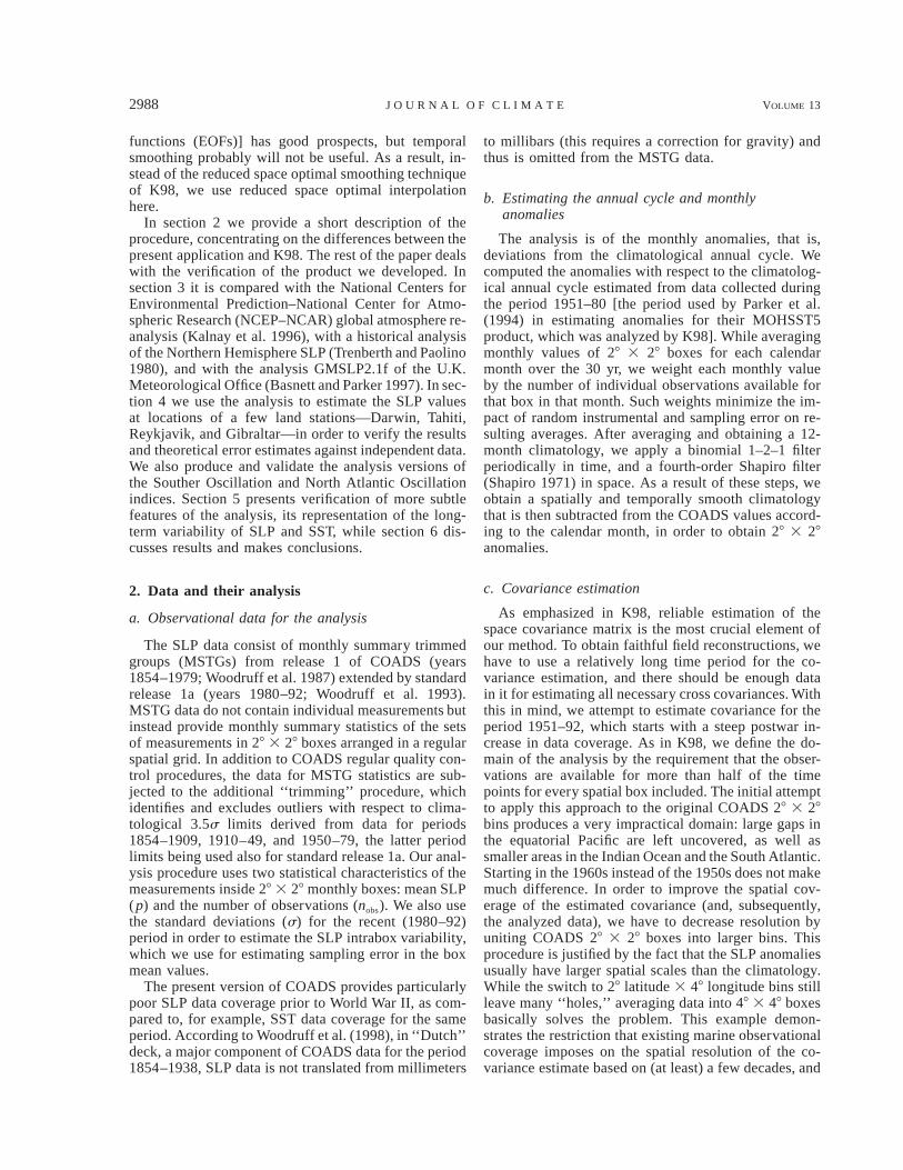
c. 1871–98

For this early period of erratic COADS data our OIanalysis differs by less than 1 mb rms from the UKMOproduct in the Tropics and is closer to the UKMO anal-ysis than to the raw COADS everywhere (Fig. 4). Infact, everywhere except for the North Atlantic and thevicinity of the New Zealand, the OI–UKMO differenceis smaller for this period than for the period 1899–1957(cf. Figs. 4b and 3c), because under the condition ofextreme data sparsity both analyses exhibit substantiallyless variance during the former period than during thelatter. The UKMO product shows particularly dramaticreduction in the variance of the analyzed anomalies:aside from the North Atlantic and New Zealand, thestandard deviation of their marine SLP anomalies rarelyexceeds 1 mb, the anomalies being equal to zero fordecades in some areas of North Pacific and SouthernHemisphere. Because of this and being based exclu-sively on the COADS data, the OI is also slightly closerto them than the UKMO product is.

It should be kept in mind that the reliability of theanalyzed SLP fields is very low for this period. Thevariance of the large-scale error alone is comparable tothe variance of reconstructed fields themselves in tropicsand North Atlantic and exceeds it in the North Pacificand Southern Ocean.

d. Equatorial Pacific

Figure 5 shows aspects of raw COADS data, theUKMO product, our OI, and SST analysis of K98 inthe annual mean anomalies for the equatorial Pacific.The OI and UKMO analyses are particularly close toeach other for the period 1960–80 and reasonably closefor the entire postwar period. For the most of the recordthe OI analysis produces an expected picture of zonallycoherent equatorial variability that mirrors variability inthe SST values. In contrast, before 1930 when theCOADS data in the area are scarce, the UKMO analysisexhibits a few patches of positive and negative anom-alies seemingly dictated by the available island stationdata. In this case the blending and smoothing techniqueemployed for the UKMO analysis could not effectivelysmooth out mean discrepancies between different sta-tions resulting in this patchy structure. The obviousshortcoming of our product is the reduction in the var-iance of the equatorial Pacific during the periods whenCOADS data are sparse (1910–20 and pre-1870).

4. Sea level pressure indicesHere we use the OI analysis of marine SLP data in

order to estimate SLP variations at locations of four

15 AUGUST 2000 2993K A P L A N E T A L .

FIG. 4. The rms differences (mb) for 1871–99 between (a) OI andCOADS, (b) OI and UKMO, and (c) UKMO and COADS.

land stations where particularly long barometric recordsare available (Table 1). The SLP records of these stationsdefine widely used climatic indices of North AtlanticOscillation (NAO) (Jones et al. 1997) and Southern Os-cillation index (SOI) (Ropelewski and Jones 1987). Weproduce marine-based proxies for a land station SLP byaveraging the OI analysis values over a few highly cor-related 48 3 48 grid boxes surrounding the station, asindicated in Table 1. Such definitions of proxies allowone to use the formalism of Kaplan et al. (1997) to getoptimal estimates of the proxies with error bars on them.Large (by far exceeding error bars) differences betweenstation data and proxies can occur in one of a few cases:when land station barometric measurements are in se-rious error, when surrounding ship data are subject tosystematic error, and when SLP on a land station has a

large contribution of essentially local effects that cannotbe captured by averaging marine SLP over the area ofa few grid boxes. Since the land station record consistsof monthly averages of many measurements taken atthe same location by the same instrument, one expectsit to be of superior quality compared to averages of shipmeasurements over individual grid boxes. Surprisingly,however, the proxies based on the latter prove to becomparable in quality with land station data, except forthe periods when marine data coverage is particularlybad.

Table 2 compares monthly time series of Darwin andTahiti SLP observations with their marine-based prox-ies. In the recent (1951–92) period of relatively reliabledata, both land station records are equally highly cor-related with the proxies and show rms deviations fromthem that are well below theoretical error estimates.Imperfections in the correspondence between stationsand proxy values in this period come mostly from high(and incoherent between the two types of records)month-to-month SLP variability. When the latter is fil-tered by a 5-month running mean filter, the match im-proves considerably (Figs. 6 and 7). For the earlier pe-riods the correspondence between the station data andproxies worsens, more so for Tahiti (where the deviationexceeds expected error) than for Darwin records. Im-provement of proxies on straight averages of local rawmarine data is remarkable (Fig. 6). In fact, the truthfulreconstructions are not even limited by the availabilityof the local data, using large-scale correlations with re-mote data in order to estimate the SLP in the vicinityof the station.

Since Darwin and Tahiti stations are known to capturethe variability of the Southern Oscillation, we expectsignificant anticorrelation of the SLP records at thesestations, as well as significant absolute values of thecorrelation with Nino-3 (mean SST for the eastern equa-torial Pacific 58S–58N, 1508–908W; we use optimal es-timates of this index from K98). We expect the absolutevalues of the correlation coefficients to be high for therecent time periods and reduced for the earlier periodsof lower quality data. Indeed, as we move from thepresent to the past the absolute values of the correlationcoefficients of station records with Nino-3 decreases:only slightly for Darwin and more appreciably for Ta-hiti. Note that the marine-based proxy for Tahiti SLPis more robust in terms of its Nino-3 correlation thanthe station record. Similarly, the two proxies are morestrongly anticorrelated with each other than the two sta-tion records.

In the spirit of Trenberth (1984), higher correlationsbetween reconstructed indices compared to the land-based ones are interpreted as higher signal-to-noise ratio(in this case ‘‘signal’’ is large-scale ENSO-associatedphenomena, ‘‘noise’’ is everything else). This improve-ment might take place for two reasons. First, a marine-based proxy might be free from systematic errors in theland station data, which, when they occur, are very dif-

2994 VOLUME 13J O U R N A L O F C L I M A T E

FIG. 5. Equatorial anomalies of (a) COADS SLP (mb), (b) UKMO (mb), (c) OI (mb), and (d) K98 SST anomaly (8C) multiplied by 21.Contour interval for SLP (SST) is 0.5 mb (0.68C); values higher than 0.25 mb (0.38C) are shaded dark, lower than 20.25 mb (20.38C)are shaded light. Missing data in (a) are dotted.

TABLE 1. Land stations and their marine proxies.

StationSource of the

land dataTime periodin the source

Marine SLP proxy defined asthe OI analysis average over the area

DarwinTahitiGibraltarReykjavik

Konnen et al. (1998)Konnen et al. (1998)Jones et al. (1997)Jones et al. (1997)

1866–19971855–19971821–19971821–1997

148–108S, 1288–1328E228–148S, 1568–1448W348–388N, 88W–48E628–668N, 288–208W

ficult to correct. For example, there are known to beproblems with the Tahiti barometer before 1935 (Ro-pelewski and Jones 1987; Trenberth and Hoar 1996).Certain biases have been corrected by Ropelewski andJones (1987) (see their Table 2). Still, the station recordshows an almost constant positive anomaly from 1928to 1932 that does not have a counterpart in either Darwin

record, Nino-3 reconstruction, or marine data abundantin the vicinity of Tahiti at that time, leading to the con-clusion that Tahiti station data are in error during theperiod. Also suspicious are the largest in this centurypositive anomaly in 1917 (incidentally, a year when thebarometer was changed; a bias correction of 2 mb wasapplied to the entire period 1917–25) and uncorrelated

15 AUGUST 2000 2995K A P L A N E T A L .

TABLE 2. Comparison of land station data with marine-based proxies at Darwin and Tahiti.

Statistics

1855–1900

Darwin Tahiti

1901–50

Darwin Tahiti

1951–92

Darwin Tahiti

Correlation between station and proxyRms diff between station and proxy (mb)Rms proxy theoretical error (mb)Correlation between proxy and Nino-3Correlation between station and Nino-3

0.451.11.30.480.51

0.261.31.1

20.4120.27

0.600.841.30.440.56

0.311.160.98

20.5320.26

0.830.601.20.610.61

0.830.560.89

20.5520.47

Correlation between proxiesCorrelation between stations

20.5520.17

20.3620.25

20.4920.35

FIG. 7. Five-month running mean SLP anomaly (mb) at Tahiti: landstation records compiled by Konnen et al. (1998) (dashed line) andRopelewski and Jones (1987) (dots), and OI proxy (solid line). Nino-3(8C) multiplied by 21 is shown by a thick light line.

FIG. 6. Five-month running mean SLP anomaly (mb) at Darwin:land station record (dashed line), OI proxy (solid line), and rawCOADS proxylike average (dots). Nino-3 (8C) is shown by a thicklight line.

with other sources variability between 1902 and 1904.Recently recovered early Tahiti data along with regres-sion of the data from other stations were used by Konnenet al. (1998) to extend the Tahitian record back to 1855and fill the gaps in it. Figure 7 shows that on both ofthe most prominent occasions of disagreement betweenKonnen et al. (1998) and Ropelewski and Jones (1987)Tahiti records (1905 and 1926), the former is closer toNino-3 and our OI estimate.

Another reason for the increase in signal-to-noise ra-

tio in the proxy indices is that our technique reconstructslarge-scale patterns of variability, and in the periods ofpoor data coverage it reflects the large-scale SouthernOscillation variability rather than local variability. Thisexplains the fact that the strongest anticorrelation be-tween proxies (20.55) is achieved in the earliest period,when the data coverage is particularly poor.

The obvious problem with the marine-based proxiesis when data availability over the entire global ocean ispoor, the optimal estimate will tend to produce no var-

2996 VOLUME 13J O U R N A L O F C L I M A T E

FIG. 8. Five-month running mean SLP anomaly (mb) at Gibraltar:land station record (dashed line), OI proxy (solid line), and rawCOADS proxylike average (dots).

FIG. 9. Five-month running mean SLP anomaly (mb) at Reykjavik:land station record (dashed line), OI proxy (solid line), and rawCOADS proxylike average (dots).

TABLE 3. Comparison of land station data with marine-based proxies at Gibraltar and Reykjavik.

Statistics

1855–1900

Gibr Reyk

1901–50

Gibr Reyk

1951–92

Gibr Reyk

Correlation between station and proxyRms diff between station and proxy (mb)Rms proxy theoretical error (mb)

0.522.32.0

0.486.35.2

0.811.41.4

0.794.23.0

0.920.981.2

0.971.72.1

Correlation between proxiesCorrelation between stations

20.5720.48

20.4820.49

20.4920.47

iability, as is the case with the Darwin and Tahiti re-constructions before 1875 (Figs. 6 and 7). This seemsto be less the case for Gibraltar and Reykjavik SLPmarine-based proxies, which take advantage of goodNorth Atlantic data coverage (Figs. 8 and 9). Otherwisethe tendencies in the Atlantic proxy correlations are con-sistent with what was observed for tropical stations(Figs. 8 and 9, and Table 3).

Figure 10 compares SOI and NAO indices based onthe proxies (seasonal and winter values respectively)with those based on land station data. The match seemsalmost perfect in the recent decades and degraded duringearlier times. This suggests that mismatches are mainly

due to the decreased data quality rather than to the dif-ference in the definition of marine-based and land-basedindices. We show monthly values of Nino-3 on SOIpanel as well. Two of the most prominent occasionswhen land-based SOI differs from the two other curves(around 1917 and 1930) are traceable to problems inthe Tahiti station record.

5. Global climate variability in the SLP analysis

Using the SLP analysis described above, and the SSTanalysis of K98, we seek to identify the leading patternsof global climate variability during the last century or

15 AUGUST 2000 2997K A P L A N E T A L .

FIG. 10. Comparison of land-based (dashed lines) and marine-based (solid lines) oscillationindices. Seasonal means for SOI and winter means for NAO are shown. SOI panel shows alsoNino-3 multiplied by 21 in a thick light line.

so. We apply a running 5-yr means filter to annual av-erages of the 80 time coefficients corresponding to SLPand SST, respectively (the direct results of the reduced-space analysis procedure), and calculate the covariancematrix between the two fields. We then perform a sin-gular value decomposition (SVD) analysis of this 80 380 covariance matrix to determine the linear combi-nations of each set of coefficients (SLP and SST) thatwould lead to time series that maximize the covariancebetween the two fields. We then regress the full data onthese time series to uncover the spatial patterns of eachfield corresponding to these modes. The procedure isequivalent to that described by Bretherton et al. (1992)and can be thought of as the latter’s reduced space ver-sion. The leading three heterogeneous patterns (the re-gression of each field on the normalized time series ofthe other) are shown in Fig. 11, and the time series arein Fig. 12.

The dominant pattern of SLP–SST covariability ex-plains 29% of the covariance, and the correlation be-tween the two corresponding time series is 0.73. To-gether, the SST time series and pattern (Fig. 12, toppanel, and Fig. 11, top left panel) describe a century-long warming of the world ocean. The SST time seriesis quite similar to that of globally averaged SST (e.g.,Nicholls et al. 1996; their Fig. 3.3). The warming is notuniform in either space or time. During the last 90 yearsor so, there are two intervals of conspicuous warming,one between 1920 and 1950, and the other after 1975or so.

The pattern is quite similar to the one described inCane et al. (1997). It indicates that most ocean areascontribute positively to the warming trend, with thestrongest warming occurring in the Southern Hemi-sphere. However, some oceanic regions display a non-committal cooling trend. These regions are found in thetropical Pacific, North Pacific, and North AtlanticOceans. Cane et al. (1997) interpret this patterns, inparticular the equatorial Pacific cooling, as the responseof the regional equatorial atmosphere–ocean system toglobal warming induced by the increase in CO2. How-ever, the robustness of the equatorial signature has beenquestioned by others (e.g., Hurrell and Trenberth 1999).The regions where the SST changes are most significant(as judged by the heterogeneous correlation patterns,not shown) are in the South Atlantic and Indian Oceans,and in the western tropical and South Pacific Ocean,west of the date line. Overall the pattern explains 11%of the analysis area SST variance.

The corresponding leading SLP time series (Fig. 12,top panel) indicates a negative trend in the last fewdecades of the nineteenth century and positive trend inthe twentieth century. The trend is disrupted by a sharpfluctuation during the World War I years, which maybe spurious. The spatial pattern of the trend (Fig. 11,top right) indicates that the east–west pressure contrastover the Pacific Ocean has been decreasing since theturn of the century. There does not seem to be a con-sistent local relationship between the trend in SLP andthat in SST. In some regions SLP is decreasing in time

2998 VOLUME 13J O U R N A L O F C L I M A T E

FIG. 11. Heterogenous regression patterns corresponding to the three leading SVD modes of SST andSLP covariance. SST patterns are in units of degrees Celsius per one standard deviation of SLP timeseries from Fig. 12; SLP patterns are in units of millibars per one standard deviation of SST time seriesfrom Fig. 12.

when SST is increasing, and in others the situation isreversed. Moreover, the pattern explains only 6% of theanalysis area SLP variance and the heterogeneous cor-relation pattern (not shown) rarely displays values high-er than 0.3, except over the southern edge of the analysisdomain. Clearly further independent SLP data are need-ed to verify the authenticity of this pattern.

The second pattern of joint SLP and SST variabilityduring the last century and a half is shown in the middleset of panels in Fig. 11. The corresponding time seriesare in the middle panel of Fig. 12. From its spatialstructure and temporal characteristics the pattern can beeasily recognized as that of the Pacific decadal oscil-lation (Zhang et al. 1997; Mantua et al. 1997). It rep-

15 AUGUST 2000 2999K A P L A N E T A L .

FIG. 12. Time series corresponding to the three leading SVDmodes for SST (8C) (solid lines) and SLP (mb) (dashed lines).

resents the low-frequency manifestation of ENSO. Thepattern entails an ‘‘ENSO-like’’ relationship betweentropical and midlatitude Pacific SST, and between SSTand SLP in the entire Pacific basin. South Atlantic andIndian Oceans SST vary in phase with those in thetropical Pacific and along the western North Americanseaboard. SLP in the Atlantic and the Indian Oceansvaries in opposite polarity to that over the northern andeastern tropical Pacific, consistent with the signature ofthe Southern Oscillation. The time series of the SLPand SST patterns are correlated at a level of 0.91 andexplain 20% of the total covariance between the twofields, and 15% and 18% of the analysis domain SSTand SLP variance, respectively. The SST time series issignificantly correlated (0.77) with the Nino-3 index,and the corresponding SLP series highly correlates(0.88) with the Trenberth and Hurrell (1994) North Pa-cific index.

The third pattern (bottom panels of Figs. 11 and 12)shows little SLP variability outside the North Atlanticbasin. The latter consists of an out-of-phase fluctuationbetween the subpolar and subtropical Atlantic, resem-bling the NAO ‘‘dipole’’ (Hurrell 1995). The corre-sponding SST pattern is more global in extent, covering

regions in both Atlantic and Pacific Ocean basins. Inthe Atlantic, SST north and south of the equator varyout of phase with each other in a manner akin to thatdisplayed by the third SST eigenvector of Folland et al.(1986) (see also Parker and Folland 1991). There is.alsosome resemblance between the North Atlantic SST pat-tern and the interdecadal pattern of Atlantic SST vari-ability described in Kushnir (1994; see also Kushnir andHeld 1996). Note that the relationship between SST andSLP variability in the North Atlantic is somewhat dif-ferent from that associated with interannual variability(Kushnir 1994; Kushnir and Held 1996). The temporalbehavior of the SLP pattern is consistent with the low-frequency evolution of the NAO index shown in Hurrell(1995) and has a correlation of 0.78 with the latter. Therelationship between Pacific SST and variability in theAtlantic basin is to some extent consistent with the Fol-land et al. (1986) analysis, but in addition reveals a linkbetween the topical Pacific and decadal changes in theNAO. However, these features maybe spurious as theSST heterogeneous correlation pattern does not displaylarge areas with correlation above 0.3, except in theNorth Atlantic and south Indian Ocean regions. As aresult this climate variability pattern explains only 6%of the SST variance. The respective number for the SLPfield is 9%. Overall this pattern explains 9% of the jointvariability of the two fields and the time series correlateat a level of 0.81.

6. Discussion and summary

This first attempt at applying the reduced space OIanalysis technique to marine SLP data shows some suc-cess. The open ocean SLP fields verify against theCDAS and UKMO analyses, products based on richerdata sources; historical reconstructions of SLP indicesare validated by land observations; the analysis errorbars give reliable error estimates; large-scale long-termmodes of variability are reasonable. However, aliasingof short-term SLP variability near land and on the south-ern edge of the analysis domain causes steep error in-crease in these areas. Comparison with other productsthat benefit from the land station data and principles ofmeteorological analysis suggests that those problemscan be helped by bringing land data into the analysis.This will be our next step, to be carried out as soon asa coherent compilation of land station SLP records cur-rently under development in the UKMO becomes avail-able for our use. Incorporating land into such an analysiswill make it almost global and will be beneficial in itsown right. We also plan to test the use of the SLP fieldsof the CDAS reanalysis for the estimation of the reducedspace patterns and energy distribution. However, thelatter procedure will result in a dependence of the anal-ysis on the CDAS assimilating model, a possible draw-back in some regions. The difference between CDASand COADS implied covariance structures, and the in-fluence of the switching from one covariance estimate

3000 VOLUME 13J O U R N A L O F C L I M A T E

to another on the results of optimal analysis, will haveto be investigated. More elaborated versions of the anal-ysis may involve seasonal variations of assumed co-variance structure and make use of SST data via SST–SLP statistical connections.

The procedure of reestimating the signal covariancedeveloped in this work achieves the consistency be-tween the energy distribution in the solution with the apriori estimate of the reduced space signal covariance.However, it apparently overestimates the covariance inthe truncated part of the spectrum. Inadequacy of theobservational data sampling and the crudeness of ourobservational error model are the most probable culprits.While the possibilities of improving the former are lim-ited, the latter can perhaps be refined in the future. Theinfluence of this procedural caveat on the present prod-uct is not particularly detrimental: if anything, it resultsin the larger (more conservative) theoretical error es-timates for the solution.

Among many things that could go wrong with thisSLP analysis is the possible aliasing of diurnal and semi-diurnal tides for the periods such as the beginning ofthe century (Barnett 1984) when the COADS data weresampled fewer than four times per day (Trenberth 1977).Effect of atmospheric tides can exceed 1 mb in theTropics, but we see no evidence of the problem in ourreconstruction of tropical indices. A possible explana-tion is that the tidal influence has a global structure ofwavenumber 2 in the atmosphere (Trenberth 1991),which is not assigned much energy by our reduced spacecovariance structure, as the latter was estimated for themodern period of approximately four times per day datasampling. Also predominant data sampling in midlati-tudes, where tidal influence is weaker, probably helpsto filter out tropical aliasing.

A surprising finding of this work is that reconstructionof SLP indices based exclusively on ship observationscan be competitive in quality with those based on landstation records. However, all presently available datasetsof marine observations start in the 1850s and have verypoor data coverage over the first two decades, whichlimits the length of useful reconstructions for marine-based indices.

Acknowledgments. We are grateful to many colleaguesfor their interest to this work and generous help. KevinTrenberth, David Parker, Phil Jones, Eugenia Kalnay, RobAllan, Mike Evans, and Scott Woodruff read the manu-script and made many useful remarks and suggestions.Constructive remarks of two anonymous reviewers areparticularly appreciated. Ed Cook discussed data avail-ability and interpretation issues; Jim Simpson explainedthe subtleties of different definitions of SOI and helpedwith the data; Klaus Wolter, Dick Reynolds, Tom Smith,and Bob Livezey discussed the results. We are thankfulto the U.K. Met. Office and Tracy Basnett for making theirSLP analysis available to us. Benno Blumenthal’s Ingridsoftware is responsible for all 2D plots in this work, and

his Data Library system uses Senya Basin’s CUF formatfor providing easy public access to the results of this workat http://ingrid.ldgo.columbia.edu/SOURCES/.KAPLAN/.RSApCOADSpSLP1.html. This work was supported byNOAA Grant UCSIO-10775411D/NA47GPO-188.

APPENDIX

Reestimation of the Signal Covariance

Kaplan et al. (1997) (hereafter K97) in their appendixB obtained equations

defpp p TA 5 ^a a & 5 L 1 P , (A1)p

defpOI OI T 21A 5 ^a a & 5 L(L 1 P ) L, (A2)OI

which tie together covariances of the projection andreduced space OI solutions (ap and aOI, respectively),error covariance for the projection solution P p, and thecovariance of the retained portion of the signal space,L, presented for the basis defined by E [cf. Eq. (1)].The projection solution ap consists of the best-fit co-efficients for the predetermined set of patterns (the col-umns of E) to the observed data. Covariance P p is thetheoretical estimate of the error in these coefficients.

The covariance L is the principal assumption in ourcomputational procedure: it determines the distributionof energy over the basis of the reduced space. If theunderlying assumptions of the method hold, the valuesof analyses covariances Ap and AOI obtained from thesolution should be approximately equal to the theoreticalvalues given by the respective right-hand sides of theequations (A1) and (A2). In particular, the covarianceof the projection solution should exceed the assumedcovariance of the ‘‘true’’ signal, while the latter shouldexceed the covariance of the OI. In K97 we tested thisconsistency by plotting the ratios of the diagonals ofthe analyses’ covariances to the diagonal of L. We ex-pect the projection ratio to be larger than unity and theOI ratio to be smaller than unity. If no adjustment ismade to the covariance found through our standard pro-cedure, this consistency check fails for the present SLPanalysis: both ratios are less than unity. This test didnot hold for the unadjusted signal covariance in our SSTanalyses either, but a heuristic procedure was introducedthat changed only the distribution of energy over theEOF modes and preserved the diagonality of L. Thisapproach implicitly assumed that the individual EOFsmodes could be used as they are, without any rotation.Results of this procedure were quite satisfactory for theSST analysis (see Fig. 15 of K97) but failed for thepresent SLP analysis. Consequently, here we develop amore complete and less heuristic procedure based onEqs. (A1) and (A2).

Inserting (A1) into (A2) to eliminate P p yields

Ap 5 L L,21AOI (A3)

in which Ap and AOI are the known estimates from the

15 AUGUST 2000 3001K A P L A N E T A L .

projection and OI solutions, respectively, and L is beingsought in the class of symmetric nonnegative definitematrices. An exact solution to the nonlinear matrix equa-tion (A3) can be constructed in the following way. Wedefine canonical decompositions of the symmetric pos-itive matrices Ap and AOI by

Ap 5 Ep , AOI 5 EOI ,2 T 22 TS E S Ep p OI OI (A4)

where Ep and EOI are orthogonal matrices, while and2Sp

are positive diagonal matrices. Inserting Eq. (A4)2SOI

into (A3) we obtain2 T 2 TE S E 5 LE S E L, orp p p OI OI OI

T T(E S )(E S ) 5 (LE S )(LE S ) .p p p p OI OI OI OI

The latter can be true if and only if there exists anorthogonal matrix U such that

EpSpU 5 LEOISOI,

and thus

L 5 EpSp .21 TUS EOI OI (A5)

Now our task is to choose U so that L defined by formula(A5) is symmetric and nonnegative definite. Symmetrymeans that

21 T 21 T TE S US E 5 E S U S E orp p OI OI OI OI p p

21 T 21 21 T 21 TUS E E S 5 S E E S UOI OI p p p P OI OI

21 T 21 T5 (US E E S ) . (A6)OI OI p p

We define the singular value decomposition ofEp by21 T 21S E SOI OI p

Ep 5 G1S ;21 T 21 TS E S GOI OI p 2 (A7)

G1 and G2 being orthogonal matrices, and S being adiagonal matrix with nonnegative elements. Obviously,the choice

U 5 G2TG1

makes

5 G2S21 T 21 TUS E E S GOI OI p p 2

symmetric and thus satisfies Eq. (A6). As a result wehave

L 5 EpSpG2S Sp ,T TG E2 p (A8)

which is obviously symmetric and nonnegative (as S isnonnegative). In order to compute the solution (A8) weperform matrix decompositions (A4) and (A7) usingMATLAB software. All matrices involved in this com-putation has the order equal to the dimension L of achosen reduced space (L 5 80 in the present applica-tion).

The entire procedure of the analysis then performedin the following two-stage way. The covariance of thefield is estimated; EOF patterns and eigenvalues arecomputed and used in projection and OI analyses with-out any adjustment. From the results of the analysis, Ap

and AOI are estimated, as is the signal covariance L,computed according to formula (A8). Canonical decom-position,

L 5 FL1FT,

shows that the EOF patterns found originally should berotated by the operator F and the distribution of energyover these rotated (but still orthogonal!) patterns shouldbe given by the elements of L1. EOFs not included intothe reduced space are not being rotated, but their ei-genvalues are modified according to the formula

5 gl i 1 c, i 5 L 1 1, . . . , M,1li

where g and c are constants that we defined from thetwo conditions: conservation of the total variance y ofthe spectrum

y 5 Tr[L1] 1 g(y 2 Tr[L]) 1 c(M 2 L),

and ‘‘no-jump’’ after the last reduced-space eigenvalue

glL11 1 c 5 .1lL

These conditions give the values of constants

1y 2 Tr[L ] 2 l (M 2 L)1 L 1g 5 , c 5 l 2 gl .L L11y 2 Tr[L] 2 l (M 2 L)L11

With this corrected estimate of covariance we rerun theanalysis and check if Eqs. (A1) and (A2) hold for Ap

and AOI estimated from its results (i.e., if the results ofthe analysis are consistent with our a priori assumptionon the signal variance). If not, we could do anotheriteration. However, for this particular SLP applicationsthe agreement was quite satisfactory.

To close the story, we examine why the heuristicalgorithm of K97 failed for the SLP analysis, but notfor the SST analysis of K98. For this we run our newcovariance reestimation algorithm for the SST analysisof K98. The explanation is that the reduced-space EOFrotation matrix F for the SLP analysis has more offdi-agonal structure than that for the SST analysis. Also theeigenvalues estimated by the present algorithm are muchcloser to those estimated by the K97 method for SSTthan for SLP.

As discussed in K97, a realistic estimate of the signalcovariance is of crucial importance for obtaining real-istic theoretical error estimates. When we repeat theexperiment with the North Atlantic 1950–92 withheldarea as in K97 and K98 we find that the theoretical errorestimate in the middle of the North Atlantic withheldarea reaches 0.8 mb, while when all the available dataare used, the estimated error is about 0.3 mb [becausethis value includes large-scale error only (Fig. 1c), ex-cluding the influence of truncation error (Fig. 1b), it issmaller than the North Atlantic error values in Fig. 2aand Table 3]. Consistent with these error estimates, therms difference between the solutions with and withoutthe data in the chosen area almost reaches 0.6 mb. Thisexample is evidence that the analysis with the given

3002 VOLUME 13J O U R N A L O F C L I M A T E

settings produces reliable conservative error estimatesfor the solution.

REFERENCES

Allan, R. J., J. A. Lindesay, and D. E. Parker, 1996: El Nino SouthernOscillation and Climatic Variability. CSIRO Publications, 405pp.

Barnett, T. P., 1984: Long-term trends in surface temperature overthe oceans. Mon. Wea. Rev., 112, 303–312.

Basnett, T. A., and D. E. Parker, 1997: Development of the globalmean sea level pressure data set GMSLP2. Hadley Centre of theU.K. Meteorological Office for Climate Research, Tech. Note79, 16 pp. [Available from the Hadley Centre for Climate Pre-diction and Research, Meteorological Office, London Road,Bracknell, Berkshire RS12 2SY, United Kingdom.]

Bottomley, M., C. K. Folland, J. Hsiung, R. E. Newell, and D. E.Parker, 1990: Global Ocean Surface Temperature Atlas. HerMajesty’s Stationery Office, 20 pp.

Bretherton, C. S., C. Smith, and J. M. Wallace, 1992: An intercom-parison of methods for finding coupled patterns in climate data.J. Climate, 5, 541–560.

Cane, M. A., A. C. Clement, A. Kaplan, Y. Kushnir, R. Murtugudde,D. Pozdnyakov, R. Seager, and S. E. Zebiak, 1997: 20th centurysea surface temperature trends. Science, 275, 957–960.

Davis, R. E., 1976: Predictability of sea surface temperature and sealevel pressure anomalies over the North Pacific Ocean. J. Phys.Oceanogr., 6, 249–266.

Folland, C. K., T. N. Palmer, and D. E. Parker, 1986: Sahel rainfalland worldwide sea temperatures 1901–85. Nature, 320, 602–607.

Hurrell, J. W., 1995: Decadal trends in the North Atlantic Oscillation:Regional temperatures and precipitation. Science, 269, 676–679., and K. E. Trenberth, 1999: Global sea surface temperatureanalyses: Multiple problems and their implications for climateanalysis, modeling, and reanalysis. Bull. Amer. Meteor. Soc., 80,2661–2678.

Jones, P. D., T. Jonsson, and D. Wheeler, 1997: Extension to the NorthAtlantic Oscillation using early instrumental pressure observa-tions from Gibraltar and South-West Iceland. Int. J. Climatol.,17, 1433–1450.

Kalnay, E., and Coauthors, 1996: The NCEP/NCAR 40-year reanal-ysis project. Bull. Amer. Meteor. Soc., 77, 437–471.

Kaplan, A., Y. Kushnir, M. A. Cane, and M. B. Blumenthal, 1997:Reduced space optimal analysis for historical datasets: 136 yearsof Atlantic sea surface temperatures. J. Geophys. Res., 102,27 835–27 860., M. A. Cane, Y. Kushnir, A. C. Clement, M. B. Blumenthal,and B. Rajagopalan, 1998: Analyses of global sea surface tem-perature 1856–1991. J. Geophys. Res., 103, 18 567–18 589.

Konnen, G. P., P. D. Jones, M. H. Kaltofen, and R. J. Allan, 1998:Pre-1866 extensions of the Southern Oscillation index using ear-

ly Indonesian and Tahitian meteorological readings. J. Climate,11, 2325–2339.

Kushnir, Y., 1994: Interdecadal variations in North Atlantic sea sur-face temperature and associated atmospheric conditions. J. Cli-mate, 7, 141–157., and I. M. Held, 1996: Equilibrium response to North AtlanticSST anomalies. J. Climate, 9, 1208–1220.

Leith, C. E., 1973: The standard error of time-average estimates ofclimatic means. J. Appl. Meteor., 12, 1066–1069.

Mantua, N. J., S. R. Hare, Y. Zhang, J. M. Wallace, and R. C. Francis,1997: A Pacific interdecadal climate oscillation with impacts onsalmon production. Bull. Amer. Meteor. Soc., 78, 1069–1079.

Nicholls, N., G. V. Gruza, J. Jouzel, T. R. Karl, L. A. Ogallo, andD. E. Parker, 1996: Observed climate variability and change.Climate Change 1995, J. T. Houghton et al., Eds., CambridgeUniversity Press, 133–192.

Parker, D. E., and C. K. Folland, 1991: Worldwide surface temper-ature trends since the mid-19th century. Greenhouse-Gas-In-duced Climatic Change: A Critical Appraisal of Simulations andObservations, M. E. Schlesinger, Ed., Elsevier, 173–193., P. D. Jones, C. K. Folland, and A. Bevan, 1994: Interdecadalchanges of surface temperature since the late nineteenth century.J. Geophys. Res., 99, 14 373–14 399.

Ropelewski, C. F., and P. D. Jones, 1987: An extension of the Tahiti–Darwin Southern Oscillation index. Mon. Wea. Rev., 115, 2161–2165.

Shapiro, R., 1971: The use of linear filtering as a parameterizationof atmospheric diffusion. J. Atmos. Sci., 28, 523–531.

Trenberth, K. E., 1977: Surface atmospheric tides in New Zealand.N. Z. J. Sci., 20, 339–356., 1984: Signal versus noise in the Southern Oscillation. Mon.Wea. Rev., 112, 326–332., 1991: Climate diagnostics from global analyses: Conservationof mass in ECMWF analyses. J. Climate, 4, 707–722., and D. A. Paolino, 1980: The Northern Hemisphere sea-levelpressure data set: Trends, errors, and discontinuities. Mon. Wea.Rev., 108, 855–872., and J. W. Hurrell, 1994: Decadal atmosphere–ocean variationsin the Pacific. Climate Dyn., 9, 303–319., and T. J. Hoar, 1996: The 1990–1995 El Nino–Southern Os-cillation event: Longest on record. Geophys. Res. Lett., 23, 57–60., J. R. Christy, and J. W. Hurrell, 1992: Monitoring global month-ly mean surface temperatures. J. Climate, 5, 1405–1423.

Woodruff, S. D., R. J. Slutz, R. L. Jenne, and P. M. Steurer, 1987:A comprehensive ocean–atmosphere data set. Bull. Amer. Me-teor. Soc., 68, 1239–1250., S. J. Lubker, K. Wolter, S. J. Worley, and J. D. Elms, 1993:Comprehensive Ocean–Atmosphere Data Set (COADS) Release1a: 1980–92. Earth Syst. Monit., 4, 1–8., H. F. Diaz, J. D. Elms, and S. J. Worley, 1998: COADS Release2 data and metadata enhancements for improvements of marinesurface flux fields. Phys. Chem. Earth, 23, 517–526.

Zhang, Y., J. M. Wallace, and D. S. Battisti, 1997: ENSO-like in-terdecadal variability: 1900–93. J. Climate, 10, 1004–1020.