Reducing Energy Costs for IBM Blue Gene/Pvia Power-Aware Job Scheduling

Zhou Zhou1, Zhiling Lan1, Wei Tang2, and Narayan Desai2

1 Department of Computer ScienceIllinois Institute of TechnologyChicago, Illinois, United States

{zzhou1,lan}@iit.edu2 Mathematics and Computer Science Division

Argonne National LaboratoryArgonne, Illinois, United States{wtang,desai}@mcs.anl.gov

Abstract. Energy expense is becoming increasingly dominant in theoperating costs of high-performance computing (HPC) systems. At thesame time, electricity prices vary significantly at different times of theday. Furthermore, job power profiles also differ greatly, especially on HPCsystems. In this paper, we propose a smart, power-aware job schedulingapproach for HPC systems based on variable energy prices and job pow-er profiles. In particular, we propose a 0-1 knapsack model and demon-strate its flexibility and effectiveness for scheduling jobs, with the goalof reducing energy cost and not degrading system utilization. We designscheduling strategies for Blue Gene/P, a typical partition-based system.Experiments with both synthetic data and real job traces from produc-tion systems show that our power-aware job scheduling approach canreduce the energy cost significantly, up to 25%, with only slight impacton system utilization.

Keywords: energy, power-aware job scheduling, resource management,Blue Gene, HPC system

1 Introduction

With the vast improvement in technology, we are now moving toward exascalecomputing. Many experts predict that exascale computers will have millions ofnodes, billions of threads of execution, hundreds of petabytes of inner memory,and exabytes of persistent storage [1]. Exascale computers will have unprece-dented scale and architectural complexity different from the petascale systemswe have now. Hence, many challenges are expected to emerge during the transi-tion to exascale computing. Four major challenges—power, storage, concurrency,and reliability—are identified where current trends in technology are insufficientand disruptive technical breakthroughs will be needed to make exascale com-puting a reality [2]. In particular, the energy and power challenge is pervasive,

affecting every part of a system. Today’s leading-edge petascale systems consumebetween 2 and 3 megawatts per petaflop [2]. It is generally accepted that an ex-aflop system should consume no more than 20 MW; otherwise their operatingcosts would be prohibitively expensive.

High-performance computing generally requires a large amount of electricityto operate computer resources and to cool the machine room. For example, ahigh-performance computing (HPC) center with 1,000 racks and about 25,000square feet requires 10 MW of energy for the computing infrastructure and anadditional 5 MW to remove the dissipated heat [3]. At the Argonne LeadershipComputing Facility (ALCF), our systems consume approximately $1 millionworth of electricity annually. As of 2006, the data centers in the United Stateswere consuming 61.4 billion kWh per year [4], an amount of energy equivalent tothat consumed by the entire transportation manufacturing industry (the indus-try that makes airplanes, ships, cars, trucks, and other means of transportation)[5]. Since the cost of powering HPC systems has been steadily rising with grow-ing performance, while the cost of hardware has remained relatively stable, itis argued that if these trends were to continue, the energy cost of a large-scalesystem during its lifetime could surpass the equipment itself [6].

Several conventional approaches to reducing energy cost have been adoptedby organizations operating HPC systems. For instance, a popular and intuitivestrategy is to manipulate the nodes within an HPC system through techniquessuch as dynamic voltage and frequency scaling, power state transitions, and theuse of separation in hot and cold aisles. Meanwhile, new cooling technologies,load-balancing algorithms, and location-aware computing have been proposedas new ways to reduce the energy demand of HPC centers [7].

In this paper we develop and analyze a new method to reduce the ener-gy cost of operating large-scale HPC systems. Our method relies on three keyobservations.

1. Electricity prices vary. In many districts in the United States with whole-sale electricity markets, the price varies on an hourly basis. Sometimes thevariation can be significant as much as a factor of 10 from one hour to thenext [7]. HPC centers often make a contract with the power companies topay variable electricity prices. A common arrangement is that HPC centerspay less for electricity consumed during an off-peak period (nighttime) thanduring an on-peak period (daytime)[4].

2. Job power consumption differs. Studies have shown that most HPC jobs havedistinct power consumption profiles. For example, in [8] the authors analyzedthe energy characteristics of the production workload at the Research CenterJuelich (FZJ) and found that their jobs have a power consumption rangingfrom 20 kW to 33 kW per rack on their Blue Gene/P system. Usually, anapplication has relatively high power consumption during its computationalphases, and its power consumption drops during the communication or I/Ophase [8]. For example, I/O-intensive jobs and computation-intensive jobshave totally different energy-consuming behaviors leading to variation intheir power consumption.

3. System utilization cannot be impacted in HPC. Most conventional power sav-ing approaches focus on manipulating nodes by turning off some nodes orputting the system into an idle phase during the peak price time. An imme-diate consequence of these approaches is that they lower system utilization[4]. Lowering system utilization for energy saving is not tolerable for HPCcenters, however. HPC systems require a significant capital investment; andhence making efficient use of expensive resources is of paramount importanceto HPC centers. Unlike Internet data centers that typically run at about 10–15% utilization, systems at HPC centers have a typical utilization of 50–80%[9], and job queues are rarely empty because of the insatiable demand in sci-ence and engineering. Therefore, an approach is needed that can save energycost while maintaining relatively high system utilization.

We argue that HPC systems can save a considerable amount of electric cost-s by adopting an intelligent scheduling policy that utilizes variable electricityprices and distinct job power profiles—without reducing system utilization. Morespecifically, we develop a power-aware scheduling mechanism that smartly selectsand allocates jobs based on their power profiles by preferentially allocating thejobs with high power consumption demands during the off-peak electricity priceperiod. Our design is built on three key techniques: a scheduling window, a 0-1knapsack model, and an on-line scheduling algorithm. The scheduling windowis used to balance different scheduling goals such as performance and fairness;rather than allocating jobs one by one from the wait queue, our scheduler makesdecisions on a group of jobs selected from the waiting queue. We formalize ourscheduling problem into a standard 0-1 knapsack model, based on which weapply dynamic programming to efficiently solve the scheduling problem. Thederived 0-1 knapsack model enables us to reduce energy cost during high elec-tricity pricing period with no or limited impact to system utilization. We useour on-line scheduling algorithm together with the scheduling window and 0-1knapsack model to schedule jobs on Blue Gene/P.

By means of trace-based simulations using real job traces of the 40-rack BlueGene/P system at Argonne, we target how much cost saving can be achievedwith this smart power-aware scheduling. One major advantage of using real jobtraces from production systems of different architectures is to ensure that exper-imental results can reflect the actual system performance to the greatest extent.Experimental results show that our scheduling approach can reduce energy bill-s by 25% with no or slight loss of system utilization and scheduling fairness.We also perform a detailed analysis to provide insight into the correlation be-tween power and system utilization rate, comparing our power-aware schedulingwith the default no-power-aware scheduling. We also conduct a sensitivity studyto explore how energy cost savings and utilization can be affected by applyingdifferent combinations of power ranges and pricing ratio.

The remainder of the paper is organized as follows. Section 2 discusses relatedstudies on HPC energy issues. Section 3 describes our methodology, includingthe scheduling window, 0-1 knapsack model, and on-line scheduling algorithm.

Section 4 describes our experiments and results. Section 5 draws conclusion andpresents future work.

2 Related Work

Research on power- or energy-aware HPC systems has been active in recent years.Broadly speaking, existing work has mainly focused on the following topics:hardware design, processor adjustment, computing nodes controlling and powercapping.

Energy-efficient hardware is being developed so that the components consumeenergy more efficiently than do standard components [10]. Several researchers[11] and [12] argue that the power consumption of a machine should be pro-portional to its workload. According to [12]a machine should consume no powerin idle state, almost no power when the workload is very light, and eventuallymore power when the workload is increased. However, power consumption doesnot strictly follow this because of the various job behaviors during runtime. In[8], the authors discuss these phenomena by presenting core power and memorypower for a job on Blue Gene/P.

Dynamic voltage and frequency scaling (DVFS) is another widely used tech-nique for controlling CPU power since the power consumption of processorsoccupies a substantial portion of the total system power (roughly 50% underload) [10]. DVFS enables a process to run at a lower frequency or voltage, in-creasing the job execution time in order to gain energy savings. Some researchefforts on applying DVFS can be found in [13], [14], and [15]. Nevertheless, D-VFS is not appropriate for some HPC systems. For example, DVFS is both lessfeasible and less important for the Blue Gene series because it does not includecomparable infrastructure and already operates at highly optimized voltage andfrequency ranges [8]. Green Destiny [16] are build based on low frequency processto achieve the goal of energy efficiency which leaves little space for DVFS whichperforms better on systems equipped with high frequency processors.

In a typical HPC system, nodes often consume considerable energy in idlestate without any running application. For example, an idle Blue Gene/P rackstill has a DC power consumption of about 13 kW. Some nodes are shut downor switched to a low-power state during the time of low system utilization [10,17]. In [13] the authors designed an approach that can dynamically turn nodeson and off during running time. Jobs are concentrated onto fewer nodes, so thatother idle nodes can be shut down to save energy consumption. Experimentson an 8-node cluster show about 19% energy savings. In their testbed, the timeused to power on the server is 100 seconds, while the time to shut down is 45seconds, causing approximately 20% degradation in performance.

Many large data centers use power capping to reduce the total power con-sumption. The data center administrator can set a threshold of power consump-tion to limit the actual power of the data center [6]. The total power consumptionis kept under a predefined power budget so that an unexpected rise in powercan be prevented. The approach also allows administrators to plan data centers

more efficiently to avoid the risk of overloading existing power supplies. Theidea of our scheduling borrows the idea of using power capping as a way to limitthe power consumption of the system. However, our work is different from theconventional power capping approach in several aspects. First, we do not controlthe total power consumption through adjusting the frequency of CPU or powerconsumption of other components. Second, our goal is not to reduce the over-all power consumption; instead, we aim at reducing energy cost by consideringvarious job power ranges and dynamic electricity prices.

3 Methodology

In this section, we present the detailed scheduling methodology. As mentionedearlier, our scheduling design is built on three key techniques: scheduling window,0-1 knapsack problem formulation, and on-line scheduling.

3.1 Problem Statement

User jobs are submitted to the system through a batch job scheduler. The jobscheduler is responsible for allocating jobs in the wait queue to compute nodes.Before performing job scheduling, we have made two essential assumptions: (1)electricity prices keep changing during the day, with significant variation betweenlow and high prices; (2) HPC jobs have different power profiles caused by differ-ent characteristics, which are available to the job scheduler at job submission.Also, our expected scheduling method should be based on the following designprinciples: (1) the scheduling method should save considerable energy cost bytaking advantage of variable electricity prices and job power profiling, (2) thereshould be no or only minor impact to system utilization, and (3) job fairnessshould be preserved as much as possible. When electricity price is high (i.e.,during the on-peak period), in order to save energy costs, we reduce the totalamount of power consumed by the jobs allocated on the system. To limit thetotal power consumption, we set an upper bound denoted as the power budgetthat the system cannot exceed. Thus, our scheduling problem is as follows: Howcan we schedule jobs with different power profiles, without exceeding a prede-fined power budget and at the same time not affecting system utilization andnot breaking the fairness of scheduling as much as possible?

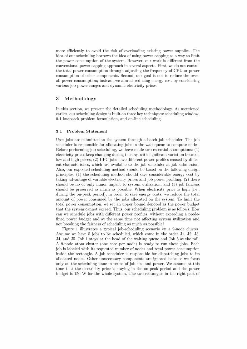
Figure 1 illustrates a typical job-scheduling scenario on a 9-node cluster.Assume we have 5 jobs to be scheduled, which come in the order J1, J2, J3,J4, and J5. Job 1 stays at the head of the waiting queue and Job 5 at the tail.A 9-node atom cluster (one core per node) is ready to run these jobs. Eachjob is labeled with its requested number of nodes and total power consumptioninside the rectangle. A job scheduler is responsible for dispatching jobs to itsallocated nodes. Other unnecessary components are ignored because we focusonly on the scheduling issue in terms of job size and power. We assume at thistime that the electricity price is staying in the on-peak period and the powerbudget is 150 W for the whole system. The two rectangles in the right part of

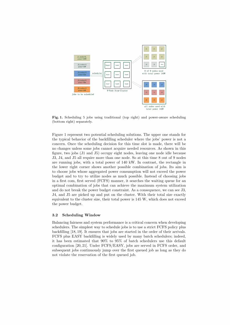
Fig. 1. Scheduling 5 jobs using traditional (top right) and power-aware scheduling(bottom right) separately.

Figure 1 represent two potential scheduling solutions. The upper one stands forthe typical behavior of the backfilling scheduler where the jobs’ power is not aconcern. Once the scheduling decision for this time slot is made, there will beno changes unless some jobs cannot acquire needed resources. As shown in thisfigure, two jobs (J1 and J5) occupy eight nodes, leaving one node idle becauseJ3, J4, and J5 all require more than one node. So at this time 8 out of 9 nodesare running jobs, with a total power of 140 kW. In contrast, the rectangle inthe lower right corner shows another possible combination of jobs. Its aim isto choose jobs whose aggregated power consumption will not exceed the powerbudget and to try to utilize nodes as much possible. Instead of choosing jobsin a first com, first served (FCFS) manner, it searches the waiting queue for anoptimal combination of jobs that can achieve the maximum system utilizationand do not break the power budget constraint. As a consequence, we can see J3,J4, and J5 are picked up and put on the cluster. With their total size exactlyequivalent to the cluster size, their total power is 145 W, which does not exceedthe power budget.

3.2 Scheduling Window

Balancing fairness and system performance is a critical concern when developingschedulers. The simplest way to schedule jobs is to use a strict FCFS policy plusbackfilling [18, 19]. It ensures that jobs are started in the order of their arrivals.FCFS plus EASY backfilling is widely used by many batch schedulers; indeed,it has been estimated that 90% to 95% of batch schedulers use this defaultconfiguration [20, 21]. Under FCFS/EASY, jobs are served in FCFS order, andsubsequent jobs continuously jump over the first queued job as long as they donot violate the reservation of the first queued job.

In our design, we use a window-based scheduling mechanism to avoid break-ing the fairness of job scheduling as much as possible. Rather than allocatingjobs one by one from the front of the queue as adopted by existing schedulers,our method allocates a window of jobs at a time. The selection of jobs into thewindow is to guarantee certain fairness, while the allocation of the jobs in thewindow onto system resources is to meet our objective of maximizing systemutilization without exceeding the predefined power budget. The job schedulermakes decisions on a group of jobs selected from the waiting queue. Jobs withinthe group are called to be in a scheduling window. To ensure fairness as muchas possible, the job scheduler selects jobs in the scheduling window based thesystem’s original scheduling policy. This can be seen as a variant of FCFS inthat this window-based approach treats the group of jobs in the front of thewait queue with the same priority.

3.3 Job Scheduling

We now describe how to formalize the scheduling problem listed in Section 3.1into a 0-1 knapsack model. We then present dynamic programming to efficientlysolve the model.

0-1 Knapsack Model Suppose there are S available nodes in the system, J jobsas {ji|1 ≤ i ≤ J} to be scheduled, and a power budget denoted as PB. Hencewe can formalize the problem into a classical 0-1 knapsack model as follows:

Problem 1. To select a subset of {ji|1 ≤ i ≤ J} such that their aggregat-ed power consumption is no more than the power budget, with the objective ofmaximizing the number of nodes allocated to these jobs.

For each job ji, we associate it with a gain value vi and weight wi. Here virepresents the number of nodes allocated to the job, which will be elaboratedin the next subsection, and wi denotes its power consumption, which is usuallymeasured in kilowatts per node or kilowatts per rack.

Problem 2. To determine a binary vector X = {xi|1 ≤ i ≤ J} such that

maximize∑

1≤i≤J

xi · vi, xi = 0 or 1

subject to∑

1≤i≤j

xi · wi ≤ PB.(1)

Job Power Profiling To make an intelligent job allocation, we must preciselymodel the job power consumption. The IBM Blue Gene series is representative ofcontiguous systems, which means that only logically contiguous subsets of nodescan be grouped to serve a single job. For instance, in Blue Gene/P systems,the basic unit of job allocation is called midplane, which includes 512 nodesconnected via a 3D torus network [22]. Two midplanes are grouped together toform a 1024-node rack. Hence a job can be allocated more nodes than it actuallyrequests.

Calculating job power consumption of a job on a contiguous system is a bitcomplicated. Because of the existence of the basic allocation unit, some nodesin the group serving a job may stay idle. Therefore, we derive the job powerconsumption as follows.

wi = Pwork nodes + Pidle nodes (2)

As shown in this equation, the total power consumption of job ji is the sumof two parts: that of the working nodes Pwork nodes and that of the idle nodesPidle nodes.

To calculate Pwork nodes and Pidle nodes, we take the Blue Gene/P system asa simple example. We get the following formulas.

Pwork nodes =Ni

Nalloci

· Pi

1024

Pidle nodes =Nalloc

i −Ni

Nalloci

· Pidle

1024

(3)

In Equation 3, Pi is the power consumption of job ji, which is measured in kWper rack; Ni is the number of nodes ji requests; and Nalloc

i is the number ofnodes ji actually get allocated. Sometimes Ni ̸= Nalloc

i because there exists abasic allocation unit (512-node midplane). Pi

1024 and Pidle

1024 denote the power con-sumption in kW/node transformed from kW/rack with a rack consisting of 1,024computing nodes. Pi and Pidle can be obtained by querying the historical dataof a job recorded by a power monitor. Many HPC systems have been equippedwith particular hardware and software to detect the running information (e.g.,LLView for Blue Gene/P; see [8]).

Dynamic Programming After setting up the gain value and weight, the 0-1knapsack model can be solved in pseudo-polynomial time by using a dynamicprogramming method [23]. To avoid redundant computation, when implementingthis algorithm we use the tabular approach by defining a 2D table G, whereG[k,w] denotes the maximum gain value that can be achieved by schedulingjobs {ji|1 ≤ i ≤ k} with no more than the power budget as w, where 1 ≤ k ≤ J .G[k,w] has the following recursive feature.

G[k,w] =

0 k = 0 or w = 0G[k − 1, w] wi ≥ wmax(G[k − 1, w], vi +G[k − 1, w − wi]) wi ≤ w

(4)

The solution G[J, PB] and its corresponding binary vector X determine theselection of jobs scheduled to run. The computation complexity of Equation 4 isO(J · PB).

3.4 On-Line Scheduling on Blue Gene/P

We apply the 0-1 knapsack model after the scheduling decision has been made.The detailed scheduling steps are as follows.

Step 1: Use a traditional scheduling method to select a set of jobs denotedas J .

Step 2: Decide whether it is an on-peak period. If so, go to Step 3. If not,set J as the optimal solution, and go to Step 5.

Step 3: Apply the 0-1 knapsack model to the job set J using weight andvalue functions, and get the optimal combination of jobs.

Step 4: Release allocated nodes of jobs that are not in the optimal set.Step 5: Start jobs in the optimal set.

Table 1. Experiment Configuration

Workload Intrepid (BG/P) at Argonne National Lab.

No. of Nodes 40,960 (40 racks)

No. of JobsMarch, 2009: 9709; Arpil, 2009: 10503May, 2009: 7925; June, 2009: 8317July, 2009: 8241; Aug, 2009: 7592

Price OeriodOn-peak(9am-11pm)Off-peak(11pm-9am)

Pricing Ratio On-peak:Off-peak = 1:3, 1:4, 1:5

Job Power Profile20 to 33 kW per rack30 to 90 kW per rack30 to 120 kw per rack

Power Budget 50%, 60%, 70%, 80%, 90%

4 Evaluation

We evaluate our power-aware scheduling algorithm by using trace-based simu-lations. In particular, we use the event-driven simulator called Qsim [24], whichsupports simulation of the BG/P system and its partition-based job scheduling.We extend Qsim to include our power-aware scheduling method. In this section,we describe the experiment configuration and our evaluation metrics. We thenpresent our experimental results by comparing our power-aware scheduling withthe default power-agnostic scheduling. Table 1 shows the overall configurationof our experiment that will be described in the next subsection.

4.1 Experiment Configuration

Job trace. Our experimental study is based on real job traces from workload-s collected from two different systems: one workload is from the 40-rack BlueGene/P system called Intrepid at Argonne. Intrepid is a partitioned torus sys-tem, so nodes can be allocated in order to connect them into a job-specific torusnetwork [25]. One major advantage of using real job traces is that experimentalresults from simulation are more convincing and can reflect the system perfor-mance to the greatest extent. For Intrepid, we use a six-month job trace from

the machine (40,960 computing nodes) collected by Cobalt, a resource managerdeveloped at Argonne [26]. It contains 52,287 jobs recorded from March 2009to August 2009. We apply our power-aware scheduling algorithm on a monthlybase to see the results for months. By doing so, we are able to examine ouralgorithm under diverse characteristics of jobs such as different numbers of jobsand various job arriving rate.Dynamic electricity price. In our experiments, we assume the most commontype of variable electricity price, namely, on-peak/off-peak pricing. Under thispricing system, electricity costs less during off-peak periods (from 11pm to 9pm)and more when used during on-peak periods (from 9am until 11pm) [4]. Here weare not concerned about the absolute value of electricity price. Instead we careonly about the ratio of on-peak pricing to off-peak pricing because one of ourgoals is to explore how much energy cost can be saved under our smart power-aware scheduling as compared with a default job scheduler without consideringpower or energy. According to the study listed in [7], the most common ratio ofon-peak and off-peak pricing varies from 2.0 to 5.0. Hence we use three differentratios, 1:3, 1:4, and 1:5, in our experiments. In the figures in the following sec-tions, we use “PR” to denote “pricing ratio” for short.Job power profile. Because we lack the power information directly related tothe testing workloads, we use the field data listed in [8] to estimate the approx-imate power consumption of jobs for our workloads. For the Intrepid workload,job power ranges between 20 to 33 kW per rack. We assign each job a randompower value within this range using normal distribution, which fits the observa-tion in [8] that most jobs fall into the 22 to 24 kW per rack range. For definitenessand without loss of generality, we apply another two sets of ranges as 30 to 90kW and 30 to 120 kW per rack. These numbers should not be taken too lit-erally since they are used to represent a higher ratio between high-power andlow-power jobs for the newest supercomputers. In the following sections, we use“power” to denote the meaning “power per rack” for short.Power budget. We evaluate five power budgets in our experiments as follows.We first run the simulation using the default scheduling policy and monitor theruntime power of the system; we then calculate the average power and set it asthe baseline value. Respectively, we set the power budget to 50%, 60%, 70%,80%, and 90% of the baseline value.

4.2 Evaluation Metrics

Our power-aware scheduling has three targets: saving energy cost, impactingsystem utilization only slightly, and preserving a certain degree of fairness.

Energy cost saving. This metric represents the amount of the energy billthat we can reduce by using our power-aware scheduling, as compared with thedefault scheduling approach without considering power or energy. In detail, theenergy cost is calculated by accumulation during runtime. Because the pricechanges at different time periods, a monitor is responsible for calculating thecurrent energy cost as an extension to Qsim.

System utilization rate. This metric represents the ratio of the utilized node-hour compared with the total available node-hours. Usually it is calculated asan average value over a specified period of time.Fairness. Currently, there is no standard way to measure job fairness. Pre-vious work on fairness of scheduling includes using “fair start time” [27] andmeasuring resource quality [28, 29]. To study the fairness of our power-awarescheduling, we propose a new metric by investigating the temporal relationshipbetween the start times of jobs. Because we adopt a scheduling window whenapply the 0-1 knapsack algorithm, Any job within this window can be selectedfor scheduling. Such scheduling may disrupt the execution order between jobsincluded in that window. Here we introduce a new metric called “inverse pair.”This idea is borrowed from the concept of permutation inverse in discrete math-ematics. In combinatorial and discrete mathematics, a pair of element of (pi, pj)is called an inversion in a permutation p if i ≥ j and pi ≤ pj [30]. Similarly,we build a sequence of jobs, S, based on their start time using a traditional jobscheduling method. Si denotes the start time of job Ji. Also we build anothersequence of jobs, called P, using our power-aware job scheduling method. In thesame way Pi denotes the start time of job Ji. In sequence S and P, for a pairof jobs Ji and Jj , if Si ≤ Sj and Pi ≥ Pj , we call jobs Ji and Jj an “inversepair.” We count the total number of inverse pairs to assess the overall fairness.This metric reflects the extent of disruption to job execution caused by usingbudget controlling.

4.3 Results

Our experimental results are presented in four different groups. First, we evaluateenergy cost saving gained by using our power-aware scheduling policy. Second, westudy the impact to system utilization after using our scheduling policy. Third,we study the extent to which scheduling fairness is impacted by our power-awarescheduling policy. We also conduct detailed analysis of how the average powerand system utilization change within a day. In the three groups above, we usethe power range 20 to 33 kW of real systems and a pricing ratio 1:3 to presentdetailed analysis. We then conduct a complementary sensitivity study on energycost savings and system utilization using different combinations of power rangesand pricing ratios.

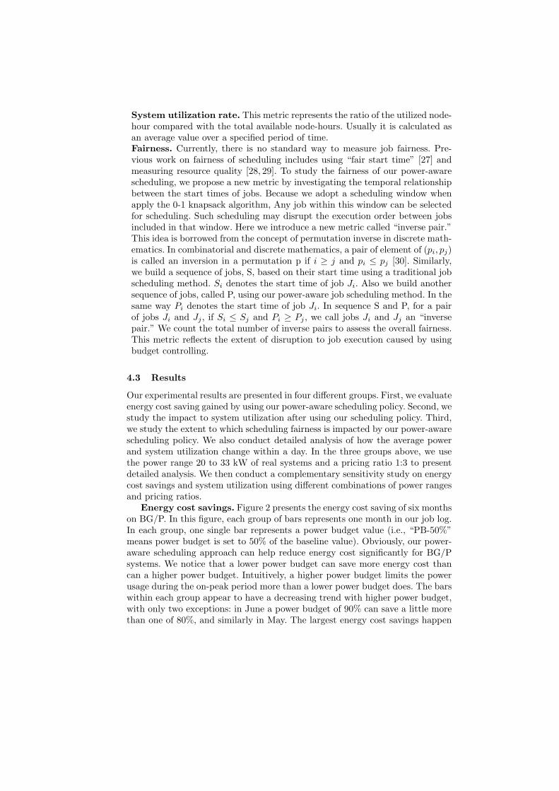
Energy cost savings. Figure 2 presents the energy cost saving of six monthson BG/P. In this figure, each group of bars represents one month in our job log.In each group, one single bar represents a power budget value (i.e., “PB-50%”means power budget is set to 50% of the baseline value). Obviously, our power-aware scheduling approach can help reduce energy cost significantly for BG/Psystems. We notice that a lower power budget can save more energy cost thancan a higher power budget. Intuitively, a higher power budget limits the powerusage during the on-peak period more than a lower power budget does. The barswithin each group appear to have a decreasing trend with higher power budget,with only two exceptions: in June a power budget of 90% can save a little morethan one of 80%, and similarly in May. The largest energy cost savings happen

0%

5%

10%

15%

20%

25%

30%

March April May June July August

Ene

rgy

cost

sav

ings

Month

PB-50% PB-60% PB-70% PB-80% PB-90%

Fig. 2. Energy cost savings with power 20 to 33 kW per rack and pricing ratio 1:3.

0%

20%

40%

60%

80%

100%

March April May June July August

Util

izat

ion

Month

PB-50%PB-60%PB-70%PB-80%PB-90%

No Power-Aware

Fig. 3. Utilization with power 20 to 33 kW per rack and pricing ratio 1:3.

in August, as much as 23% with a power budget of 50%. For the other fivemonths, using a power budget of 50% can achieve more than 15% cost savings.Even when using the highest power budget (PB-90%), most months can achievemore than 5% energy cost savings.

Impact on utilization. Figure 3 shows the system utilization of six monthson BG/P. The bars are similar to those in Figure 2, and in each group there is anadditional bar for the default scheduling method without power-aware schedul-ing. The figure shows that the system utilization is roughly 50% to 70%, whichis comparable to many real scientific computing data centers and grids [31, 12].Two features are prominent. First we observe that our power-aware schedulingapproach only slightly affects the system utilization rate. Unlike energy costsavings, the disparity between high and low power budget is not large, com-pared with the base value. For example, the most utilization drop is in Junewhen the original utilization rate using default scheduling policy is around 75%,while using a power budget of 50% results in a utilization rate of 62%. Second,whereas five power budgets are used in July, the utilization rates are almost thesame, around 55%. This phenomenon is caused by our power-aware schedulingapproach, which shifts some of the workload from the on-peak period to the off-peak period. We note that using a power budget would affect the utilization rate

0

1000

2000

3000

4000

5000

6000

7000

8000

9000

10000

50% 60% 70% 80% 90%

Num

ber

of in

vers

e pa

irs

Power budget (kW)

March, 2009April, 2009May, 2009

June, 2009July, 2009

August, 2009

Fig. 4. Fairness of scheduling under power range 20 to 33 kW per rack and pricingratio 1:3.

only during the on-peak period and would be compensated during the off-peakperiod.

Impact on fairness. We assess the fairness of scheduling using the metric“inverse pair.” Her we evaluate how the power budget will affect the fairness ofjob scheduling. Figure 4 depicts the total number of inverse pairs on BG/P. Thex-axis represents the power budget as introduced in the simulation configurationsection. The y-axis denotes the total number of inverse pairs when we imposedifferent power budgets. First we found that the number of inverse pairs occupiesonly a small portion of the total number of job pairs. For example, when we usea 50% power budget job log from March 2009 on BG/P, the number of inversepairs is nearly 7,000, and the total number of job pairs in the job sequence isabout 107 (9,709 jobs and C2

9709 ≈ 108). From Figure 4 we can clearly see thatthe number of inverse pairs decreases as the power budget goes up; generally,the trend shows a linear decline as the power budget grows up. Even under thelowest power budget (50%) the total order of job executions is not affected toomuch, with the number of inverse pairs up to 8,000. Moreover, for all months,the number of inverse pairs dropped by nearly 50% when the power budget rosefrom 50% to 60%. We found that the number of inverse pairs is also related to thenumber of jobs in the job trace. Intuitively, a larger power budget is beneficial toscheduling more jobs and not disrupting their relatively temporal relationship.

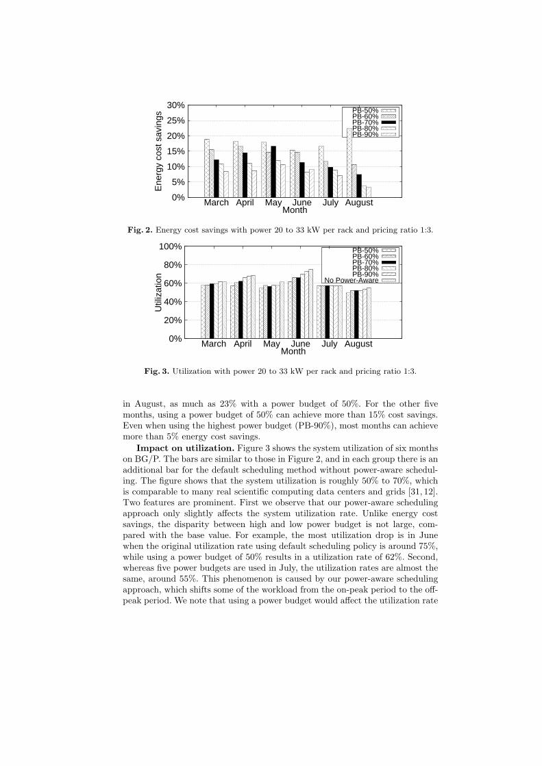
Correlation between power and utilization. So far, we have studied theenergy cost savings and system utilization rate under our power-aware schedulingapproach. Here we present detailed results of the power and instant utilizationwithin a day and how power-aware scheduling affects them. Figure 5(a) showsthe average power in a day during March 2009 of a BG/P job trace. The x-axisrepresents the time in one day measured in minute. The y-axis represents theinstant system power consumption recorded at each time point. The black lineabove minute=540 splits the time of a day into two periods of which the leftpart represents the off-peak period, whereas the right parts represents on-peakperiod. The green line represents a traditional system power pattern using thedefault scheduling policy. This reflects a common behavior of system power withrelatively low power consumption early in the morning and higher during the restof the day. Remember that in our simulation configuration, we set the on-peak

0

200

400

600

800

1000

1200

0 200 400 600 800 1000 1200 1400

Pow

er (

kilo

wat

t)

Time of day (minute)

Off-peak period On-peak period PB-50%, Price-1:3No Power-Aware

(a) Daily power on average during March 2009

0%

20%

40%

60%

80%

100%

0 200 400 600 800 1000 1200 1400

Util

izat

ion

Time of day (minute)

Off-peak period On-peak period PB-50%, Price-1:3No Power-Aware

(b) Daily utilization on average during March 2009

Fig. 5. Average power and utilization of BG/P using default no power-aware jobscheduling (green line) power 20 to 33 kW per rack and pricing ratio 1:3 (red line).

period to be 9am to 11pm. Hence, we find that the system power with power-aware scheduling (red line) starts to go down around the time where minute=540.We can see that the red line is always below around 50% of the baseline valueas half of the power of the green line. And we can also see that during the off-peak period where minute goes from 0 to 540, the system is running at a higherpower rate indicated by the red line. The reason is that along with power-awarescheduling during on-peak period some jobs are delayed and get a chance to berun after on-peak period. These jobs can be seen as being “pushed” to off-peakperiod. This situation leads to more jobs in the waiting queue, causing morepower consumption than the original scheduling method does. This fits what weexpect, namely, that during the on-peak period less energy should be consumedand during the off-peak period more energy should be consumed.

Figure 5(b) shows the average utilization within a day for job log March2009. The black dashed line where minutes=540 still acts as the splitting pointbetween off-peak period and on-peak period. Obviously, we can see the curveof the utilization line conforms very closely to that in Figure 5(a). This fits theconclusion of multiple studies [6, 12] which have indicated that CPU utilizationis a good estimator for power usage. First we examine the left part of the dashedline. Beginning from minute=540, the system utilization under default schedulingfluctuates around 80% and has a small drop off to 70% later on. This is typical inthe real world because systems are always highly utilized in daytime where more

0%

5%

10%

15%

20%

25%

30%

March April May June July August

Ene

rgy

cost

sav

ings

Month

PB-50% PB-60% PB-70% PB-80% PB-90%

(a) Power 30-90 kW, PR 1:3

0%

5%

10%

15%

20%

25%

30%

March April May June July August

Ene

rgy

cost

sav

ings

Month

PB-50% PB-60% PB-70% PB-80% PB-90%

(b) Power 30-120 kW, PR 1:3

0%

5%

10%

15%

20%

25%

30%

March April May June July August

Ene

rgy

cost

sav

ings

Month

PB-50% PB-60% PB-70% PB-80% PB-90%

(c) Power 30-90 kW, PR 1:4

0%

5%

10%

15%

20%

25%

30%

March April May June July August

Ene

rgy

cost

sav

ings

Month

PB-50% PB-60% PB-70% PB-80% PB-90%

(d) Power 30-120 kW, PR 1:4

0%

5%

10%

15%

20%

25%

30%

March April May June July August

Ene

rgy

cost

sav

ings

Month

PB-50% PB-60% PB-70% PB-80% PB-90%

(e) Power 20-33 kW, PR 1:4

0%

5%

10%

15%

20%

25%

30%

March April May June July August

Ene

rgy

cost

sav

ings

Month

PB-50% PB-60% PB-70% PB-80% PB-90%

(f) Power 30-90 kW, PR 1:5

0%

5%

10%

15%

20%

25%

30%

March April May June July August

Ene

rgy

cost

sav

ings

Month

PB-50% PB-60% PB-70% PB-80% PB-90%

(g) Power 30-120 kW, PR 1:5

0%

5%

10%

15%

20%

25%

30%

March April May June July August

Ene

rgy

cost

sav

ings

Month

PB-50% PB-60% PB-70% PB-80% PB-90%

(h) Power 20-33 kW, PR 1:5

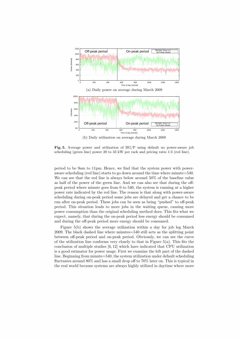
Fig. 6. Energy cost savings under various combinations; “Power” is the power rangeper rack, and “PR” is the pricing ratio.

jobs are submitted into the system. Also from minute=540, system utilizationunder power-aware scheduling policy starts to drop off and swiftly reaches arelatively stable value about 40% to 50%. Now we refer to the right part denotingthe off-peak period. As shown in Figure 8, the green line and red line resemblethe tendency in Figure 7. The utilization use power-aware scheduling is higherthan scheduling without power budget most of the time. Overall, our power-aware scheduling approach reduces the system utilization during on-peak periodand on the contrary raise it during off-peak period as compensation. Hence, ithas only a slight impact on the whole system utilization, as we presented in theprevious section.

Sensitivity study Our initial profiling experiments show that in future sys-tems the difference of job power consumption is expected to be higher. Today’sleadership-class supercomputers have wider power ranges, where the ratio be-

0%

20%

40%

60%

80%

100%

March April May June July August

Util

izat

ion

Month

PB-50%PB-60%PB-70%PB-80%PB-90%

No Power-Aware

(a) Power 30-90 kW, PR 1:3

0%

20%

40%

60%

80%

100%

March April May June July August

Util

izat

ion

Month

PB-50%PB-60%PB-70%PB-80%PB-90%

No Power-Aware

(b) Power 30-120 kW, PR 1:3

0%

20%

40%

60%

80%

100%

March April May June July August

Util

izat

ion

Month

PB-50%PB-60%PB-70%PB-80%PB-90%

No Power-Aware

(c) Power 30-90 kW, PR 1:4

0%

20%

40%

60%

80%

100%

March April May June July August

Util

izat

ion

Month

PB-50%PB-60%PB-70%PB-80%PB-90%

No Power-Aware

(d) Power 30-120 kW, PR 1:4

0%

20%

40%

60%

80%

100%

March April May June July August

Util

izat

ion

Month

PB-50%PB-60%PB-70%PB-80%PB-90%

No Power-Aware

(e) Power 20-33 kW, PR 1:4

0%

20%

40%

60%

80%

100%

March April May June July August

Util

izat

ion

Month

PB-50%PB-60%PB-70%PB-80%PB-90%

No Power-Aware

(f) Power 30-90 kW, PR 1:5

0%

20%

40%

60%

80%

100%

March April May June July August

Util

izat

ion

Month

PB-50%PB-60%PB-70%PB-80%PB-90%

No Power-Aware

(g) Power 30-120 kW, PR 1:5

0%

20%

40%

60%

80%

100%

March April May June July August

Util

izat

ion

Month

PB-50%PB-60%PB-70%PB-80%PB-90%

No Power-Aware

(h) Power 20-33 kW, PR 1:5

Fig. 7. Utilization under various combinations; “Power” is the power range per rackand “PR” is the pricing ratio.

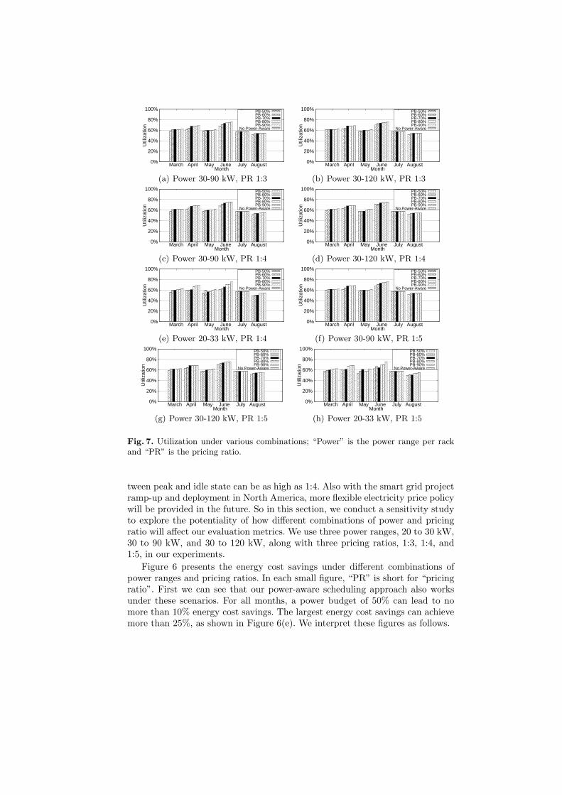
tween peak and idle state can be as high as 1:4. Also with the smart grid projectramp-up and deployment in North America, more flexible electricity price policywill be provided in the future. So in this section, we conduct a sensitivity studyto explore the potentiality of how different combinations of power and pricingratio will affect our evaluation metrics. We use three power ranges, 20 to 30 kW,30 to 90 kW, and 30 to 120 kW, along with three pricing ratios, 1:3, 1:4, and1:5, in our experiments.

Figure 6 presents the energy cost savings under different combinations ofpower ranges and pricing ratios. In each small figure, “PR” is short for “pricingratio”. First we can see that our power-aware scheduling approach also worksunder these scenarios. For all months, a power budget of 50% can lead to nomore than 10% energy cost savings. The largest energy cost savings can achievemore than 25%, as shown in Figure 6(e). We interpret these figures as follows.

First, we compare energy cost savings under variable power ranges and fixedpricing ratios. We observe that a narrower power range is likely to save moreenergy cost savings than is a wider power range. For example, when the pricingratio is fixed to 1:4, the effect of a power range of 20 to 33 kW is greater thanthat of power range 30 to 90 kW and 30 to 120 kW in all months. Also under thesame pricing ratio 1:4, a power range 30 to 90 kW results in greater energy costsavings than in almost all the months with a power range of 30 to 120 kW. Thereason is that the majority of jobs in the BG/P log are small and thus requirenodes less than 2 racks, which can have many more idle nodes. With many smalljobs running in the systems, the system power tends to be lower than on systemswhere job sizes are more uniformly distributed. As a result, imposing a powerbudget cannot constrain the power of the whole system as much as that undera narrower power range.

Second, we focus on savings under a fixed power range and variable pricingratio. Obviously, higher pricing ratios produce more energy cost savings in everymonth. Since some portion of the system power usage is shifted from the on-peakperiod to the off-peak period, higher pricing ratios lead to more difference in thecost of the amount of power transferred. Hence we believe one can saving saveenergy costs with a personalized electricity pricing policy in the future.

Figure 7 shows the system utilization rates under different combinations ofpower ranges and pricing ratios. Since the pricing ratio does not influence theutilization, we focus only on variable power ranges. First, similar to Figure 3, ourpower-aware job scheduling brings minor impact to system utilization rate. Thelargest utilization drop is in June in Figure 7(e), a drop of about 15%. Second,we observe that system utilization rates under wider power ranger are higher insome months. For example, in Figure 7(g) when the price is fixed at 1:5, usinga power range of 30 to 120 kW gives rise to higher utilization in June than doesa power range of 20 to 33 kW. This result reflects the role of our 0-1 knapsackalgorithm. Under the same power budget, a wider power range can generate amore optimal solution because of the larger choosing space. But we notice thatthe effect is not that obvious because in BG/P the system resources released byjobs each time are relatively small compared with the whole system size, thusleaving little space for optimizing the system utilization rate.

4.4 Results Summary

In summary, our trace-based experiments have shown the following.

• Our power-aware scheduling approach can effectively reduce the energy costby up to 25%. For HPC centers such as the ALCF, this energy cost savings istranslated into over $250,000 saving per year.

• This energy cost savings comes at the expense of a slight impact on systemutilization during the on-peak price period. We also observe a modest increasein system utilization during the off-peak price period. In other words, theoverall system utilization does not change much on a daily base.

• While our scheduling window preserves some degree of scheduling fairness,some jobs, especially those having high power consumption, will be delayed;but the delay is limited to a day.

• Based on our sensitivity study, we find that our power-aware job schedulinghas a high potential to save energy costs and maintain system utilization.

5 Conclusion and Future Work

In this paper, we have presented a smart power-aware scheduling method toreduce electric bills for HPC systems under the condition of limiting the impacton system utilization and scheduling fairness. The design explores variable elec-tricity prices and distinct job power profiles. Our approach contains three keytechniques: a scheduling window, 0-1 knapsack, and on-line scheduling algorithm.Using real workloads from BG/P, we have demonstrated that our power-awarescheduling can effectively save energy costs with acceptable loss to system met-rics such as utilization.

This is our first step in investigating power-aware job scheduling to addressthe energy challenge for HPC. We plan to extend our work in several ways. First,we will explore data analysis technology on historical data in order to examinepower profiles for HPC jobs at various production systems; our aim is to en-able us to predict job power profiles at their submission. Additionally, we areenhancing our power-aware scheduling with an adaptive self-tuning mechanism;the resulting job scheduler will be able to adjust its decision to external condi-tions such as electricity price automatically during operation. We also plan tointegrate this work with our prior studies on fault-aware scheduling [24, 21, 32].

Acknowledgment

This work was supported in part by the U.S. National Science Foundation grantsCNS-0834514 and CNS-0720549 and in part by the U.S. Department of Ener-gy, Office of Science, Advanced Scientific Computing Research under contractDE-AC02-06CH1135. We thank Dr. Ioan Raicu for generously providing high-performance servers for our experiments.

References

1. Z. Zhou, W. Tang, Z. Zheng, Z. Lan, and N. Desai, “Evaluating performanceimpacts of delayed failure repairing on large-scale systems,” in 2011 IEEE Inter-national Conference on Cluster Computing (CLUSTER), pp. 532–536, 2011.

2. K. Bergman, S. Borkar, D. Campbell, W. Carlson, W. Dally, M. Denneau, P. Fran-zon, W. Harrod, J. Hiller, S. Karp, S. Keckler, D. Klein, R. Lucas, M. Richard-s, A. Scarpelli, S. Scott, A. Snavely, T. Sterling, R. S. Williams, K. Yelick,K. Bergman, S. Borkar, D. Campbell, W. Carlson, W. Dally, M. Denneau, P. Fran-zon, W. Harrod, J. Hiller, S. Keckler, D. Klein, P. Kogge, R. S. Williams, andK. Yelick, “Exascale computing study: Technology challenges in achieving exas-cale systems,” 2008.

3. C. Patel, R. Sharma, C. Bash, and S. Graupner, “Energy aware grid: Global work-load placement based on energy efficiency,” in Proceedings of IMECE, 2003.

4. I. Goiri, K. Le, M. Haque, R. Beauchea, T. Nguyen, J. Guitart, J. Torres, andR. Bianchini, “Greenslot: Scheduling energy consumption in green datacenters,”in 2011 International Conference on High Performance Computing, Networking,Storage and Analysis (SC), pp. 1–11, 2011.

5. A. Jossen, J. Garche, and D. U. Sauer, “Operation conditions of batteries in pvapplications,” Solar Energy, vol. 76, pp. 759–769, 2004.

6. X. Fan, W.-D. Weber, and L. A. Barroso, “Power provisioning for a warehouse-sized computer,” in Proceedings of the 34th annual International Symposium onComputer Architecture, ISCA ’07, (New York, NY, USA), pp. 13–23, ACM, 2007.

7. A. Qureshi, R. Weber, H. Balakrishnan, J. Guttag, and B. Maggs, “Cutting theelectric bill for internet-scale systems,” in Proceedings of the ACM SIGCOMM2009 conference on data communication, SIGCOMM ’09, (New York, NY, USA),pp. 123–134, ACM, 2009.

8. M. Hennecke, W. Frings, W. Homberg, A. Zitz, M. Knobloch, and H. Bttiger,“Measuring power consumption on IBM Blue Gene/P,” Computer Science - Re-search and Development, vol. 27, no. 4, pp. 329–336, 2012.

9. “Parallel workload archive.” http://www.cs.huji.ac.il/labs/parallel/workload/.10. O. Mmmel, M. Majanen, R. Basmadjian, H. Meer, A. Giesler, and W. Homberg,

“Energy-aware job scheduler for high-performance computing,” Computer Science- Research and Development, vol. 27, no. 4, pp. 265–275, 2012.

11. D. Meisner, C. Sadler, L. Barroso, W. Weber, and T. Wenisch, “Power managementof online data-intensive services,” in 2011 38th Annual International Symposiumon Computer Architecture (ISCA), pp. 319–330, 2011.

12. L. Barroso and U. Holzle, “The case for energy-proportional computing,” Comput-er, vol. 40, no. 12, pp. 33–37, 2007.

13. E. Pinheiro, R. Bianchini, E. V. Carrera, and T. Heath, “Load balancing andunbalancing for power and performance in cluster-based systems,” in Proceedingsof the Workshop on Compilers and Operating Systems for Low Power (COLP’01),2001.

14. Y. Liu and H. Zhu, “A survey of the research on power management techniques forhigh-performance systems,” Softw. Pract. Exper., vol. 40, pp. 943–964, Oct. 2010.

15. E. Lee, I. Kulkarni, D. Pompili, and M. Parashar, “Proactive thermal managementin green datacenters,” The Journal of Supercomputing, vol. 60, no. 2, pp. 165–195,2012.

16. W. Feng, M. Warren, and E. Weigle, “The bladed beowulf: a cost-effective alterna-tive to traditional beowulfs,” in Proceedings. 2002 IEEE International Conferenceon Cluster Computing, 2002, pp. 245–254, 2002.

17. J. Hikita, A. Hirano, and H. Nakashima, “Saving 200kw and $200k/year by power-aware job/machine scheduling,” in IEEE International Symposium on Parallel andDistributed Processing, 2008, IPDPS 2008, pp. 1–8, 2008.

18. Y. Etsion and D. Tsafrir, “A short survey of commercial cluster batch schedulers,”tech. rep., The Hebrew University of Jerusalem, Jerusalem, Israel, May 2005.

19. D. Feitelson and A. Weil, “Utilization and predictability in scheduling the ibmsp2 with backfilling,” in Parallel Processing Symposium, 1998. IPPS/SPDP 1998.Proceedings of the First Merged International ... and Symposium on Parallel andDistributed Processing 1998, pp. 542–546, 1998.

20. D. Tsafrir, Y. Etsion, and D. Feitelson, “Backfilling using system-generated pre-dictions rather than user runtime estimates,” IEEE Transactions on Parallel andDistributed Systems, vol. 18, no. 6, pp. 789–803, 2007.

21. Y. Li, Z. Lan, P. Gujrati, and X.-H. Sun, “Fault-aware runtime strategies for high-performance computing,” Parallel and Distributed Systems, IEEE Transactions on,vol. 20, no. 4, pp. 460–473, 2009.

22. “Overview of the IBM Blue Gene/P project,” IBM Journal of Research and De-velopment, vol. 52, no. 1.2, pp. 199–220, 2008.

23. T. H. Cormen, C. Stein, R. L. Rivest, and C. E. Leiserson, Introduction to Algo-rithms. McGraw-Hill Higher Education, 2nd ed., 2001.

24. W. Tang, Z. Lan, N. Desai, and D. Buettner, “Fault-aware, utility-based jobscheduling on Blue Gene/P systems,” in IEEE International Conference on ClusterComputing and Workshops, 2009, CLUSTER ’09, pp. 1–10, 2009.

25. W. Tang, Z. Lan, N. Desai, D. Buettner, and Y. Yu, “Reducing fragmentation ontorus-connected supercomputers,” in 2011 IEEE International Parallel DistributedProcessing Symposium (IPDPS), pp. 828–839, May 2011.

26. “Cobalt resource manager.” http://trac.mcs.anl.gov/projects/cobalt.27. G. Sabin, G. Kochhar, and P. Sadayappan, “Job fairness in non-preemptive job

scheduling,” in International Conference on Parallel Processing, 2004, ICPP 2004,pp. 186–194, vol. 1, 2004.

28. G. Sabin and P. Sadayappan, “Unfairness metrics for space-sharing parallel jobschedulers,” in Job Scheduling Strategies for Parallel Processing (D. Feitelson,E. Frachtenberg, L. Rudolph, and U. Schwiegelshohn, eds.), vol. 3834 of LectureNotes in Computer Science, pp. 238–256, Springer, Berlin, 2005.

29. W. Tang, D. Ren, Z. Lan, and N. Desai, “Adaptive metric-aware job schedulingfor production supercomputers,” in Parallel Processing Workshops (ICPPW), 201241st International Conference on, pp. 107–115, 2012.

30. S. Pemmaraju and S. Skiena, Computational Discrete Mathematics:Combinatoricsand Graph Theory with Mathematica. New York, NY, USA: Cambridge UniversityPress, 2003.

31. I. Rodero, F. Guim, and J. Corbalan, “Evaluation of coordinated grid schedulingstrategies,” in 11th IEEE International Conference on High Performance Comput-ing and Communications, 2009, HPCC ’09, pp. 1–10, 2009.

32. W. Tang, N. Desai, D. Buettner, and Z. Lan, “Analyzing and adjusting user run-time estimates to improve job scheduling on the Blue Gene/P,” in IEEE Inter-national Symposium on Parallel Distributed Processing (IPDPS), 2010, pp. 1–11,2010.

Government License

The submitted manuscript has been created by UChicago Argonne, LLC, Opera-tor of Argonne National Laboratory (”Argonne”). Argonne, a U.S. Departmentof Energy Office of Science laboratory, is operated under Contract No. DE-AC02-06CH11357. The U.S. Government retains for itself, and others acting onits behalf, a paid-up nonexclusive, irrevocable worldwide license in said article toreproduce, prepare derivative works, distribute copies to the public, and performpublicly and display publicly, by or on behalf of the Government.