Reducing the thermal conductivity of chemically ordered binary alloys below the1

alloy limit via the alteration of phonon dispersion relations – supporting2

information3

Ashutosh Giri,1 Jeffrey L. Braun,1 John A. Tomko,1 and Patrick E. Hopkins1, a)4

Department of Mechanical and Aerospace Engineering, University of Virginia,5

Charlottesville, Virginia 22904, USA6

(Dated: May 3, 2017)7

a)Electronic mail: phopkins@virginia.edu

1

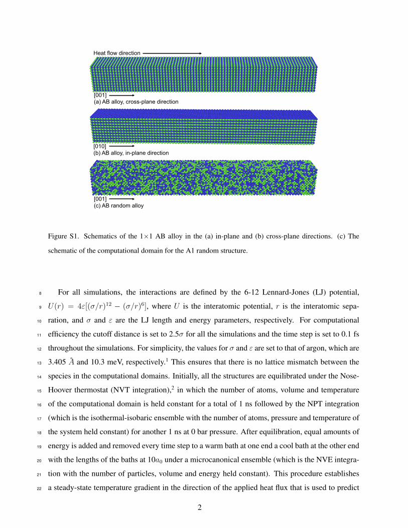
[001] (a) AB alloy, cross-plane direction

[010] (b) AB alloy, in-plane direction

[001] (c) AB random alloy

Heat flow direction

Figure S1. Schematics of the 1×1 AB alloy in the (a) in-plane and (b) cross-plane directions. (c) The

schematic of the computational domain for the A1 random structure.

For all simulations, the interactions are defined by the 6-12 Lennard-Jones (LJ) potential,8

U(r) = 4ε[(σ/r)12 − (σ/r)6], where U is the interatomic potential, r is the interatomic sepa-9

ration, and σ and ε are the LJ length and energy parameters, respectively. For computational10

efficiency the cutoff distance is set to 2.5σ for all the simulations and the time step is set to 0.1 fs11

throughout the simulations. For simplicity, the values for σ and ε are set to that of argon, which are12

3.405 A and 10.3 meV, respectively.1 This ensures that there is no lattice mismatch between the13

species in the computational domains. Initially, all the structures are equilibrated under the Nose-14

Hoover thermostat (NVT integration),2 in which the number of atoms, volume and temperature15

of the computational domain is held constant for a total of 1 ns followed by the NPT integration16

(which is the isothermal-isobaric ensemble with the number of atoms, pressure and temperature of17

the system held constant) for another 1 ns at 0 bar pressure. After equilibration, equal amounts of18

energy is added and removed every time step to a warm bath at one end a cool bath at the other end19

with the lengths of the baths at 10a0 under a microcanonical ensemble (which is the NVE integra-20

tion with the number of particles, volume and energy held constant). This procedure establishes21

a steady-state temperature gradient in the direction of the applied heat flux that is used to predict22

2

the thermal conductivity by invoking the Fourier law, Q = −κ∂T/∂z, where the applied flux is in23

the z-direction.24

Figure 2a of the manuscript shows the temperature dependent thermal conductivities of ma-25

terials A and B calculated along the [001] direction, the thermal conductivity of the AB alloy in26

the in-plane and cross-plane directions, and the thermal conductivity of the disordered (random27

alloy). Figure S1 shows the schematics of the computational domains for the 1×1 AB alloy in28

the cross-plane and in-plane direction, along with the schematic of its constituent A1 random al-29

loy structure. To ensure that size effects did not affect the thermal conductivity calculations, we30

implemented two pre-equilibrated domain sizes (with Lz=60 and 80 UCs). As the thermal con-31

ductivity predictions do not show a systematic change with the domain size, finite size effects can32

be ruled out in our simulations. Also, to gain confidence in our NEMD predictions, we compare33

the thermal conductivity calculations for our LJ argon structure with that predicted via the Green-34

Kubo (GK) technique in Ref. 3. The agreement between our NEMD predictions and the that of35

the GK simulations further supports our claim that no size effects distort our calculations. The36

error bars represent uncertainties in the fitting routine from three independent simulations and un-37

correlated fluctuations in the data sampling for all computational domains. It should also be noted38

that increasing the applied heat flux or changing the direction of the heat flow did not produce39

statistically significant change in the thermal conductivity calculations.40

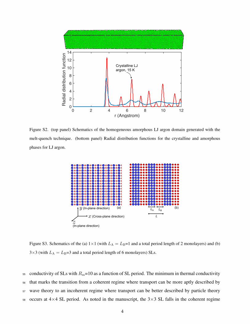
The amorphous phases were generated using the melt-quench technique. Starting from a solid41

arranged in an fcc lattice with a0=5.31 A, the crystal is heated from 0 to 300 K (note the melting42

temperature of LJ argon is 87 K) via a velocity scaling routine. To lose all memory of the initial43

conditions, the liquid is equilibrated at 300 K temperature for a total of 500 ps. After equilibration,44

the structures are rapidly cooled to 4 K at a quench rate of 0.8 K/ps. Further equilibration is per-45

formed under the NPT integration at 0 bar pressure for a total of 1 ns to obtain the final amorphous46

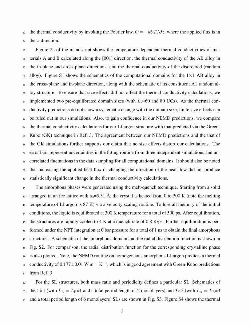
structures. A schematic of the amorphous domain and the radial distribution function is shown in47

Fig. S2. For comparison, the radial distribution function for the corresponding crystalline phase48

is also plotted. Note, the NEMD routine on homogeneous amorphous LJ argon predicts a thermal49

conductivity of 0.177±0.01 W m−1 K−1, which is in good agreement with Green-Kubo predictions50

from Ref. 351

For the SL structures, both mass ratio and periodicity defines a particular SL. Schematics of52

the 1×1 (with LA = LB=1 and a total period length of 2 monolayers) and 3×3 (with LA = LB=353

and a total period length of 6 monolayers) SLs are shown in Fig. S3. Figure S4 shows the thermal54

3

0 2 4 6 8 10 12r (Angstrom)

0

2

4

6

8

10

12

14

Rad

ial d

istri

butio

n fu

nctio

nCrystalline LJ argon, 15 K

Figure S2. (top panel) Schematics of the homogeneous amorphous LJ argon domain generated with the

melt-quench technique. (bottom panel) Radial distribution functions for the crystalline and amorphous

phases for LJ argon.

LA

LB

L

(Cross-plane direction)

(In-plane direction)

(In-plane direction)

zx

y (a)

(b)

Figure S3. Schematics of the (a) 1×1 (with LA = LB=1 and a total period length of 2 monolayers) and (b)

3×3 (with LA = LB=3 and a total period length of 6 monolayers) SLs.

conductivity of SLs withRm=10 as a function of SL period. The minimum in thermal conductivity55

that marks the transition from a coherent regime where transport can be more aptly described by56

wave theory to an incoherent regime where transport can be better described by particle theory57

occurs at 4×4 SL period. As noted in the manuscript, the 3×3 SL falls in the coherent regime58

4

0 5 10 15

Period (monolayers)

0

0.02

0.04

0.06

0.08

0.1

Therm

al C

onductivity (

W m

-1 K

-1)

minimum limit, Rm

= 10

Rm

= 10

Figure S4. Thermal conductivity of SLs with Rm=10 as a function of SL period (in monolayers). For

comparison, the thermal conductivity of the corresponding amorphous phase is also shown.

where the reduced thermal conductivity is a result of zone folding and miniband formation. The59

minimum in the SL thermal conductivity is well below the theoretical minimum corresponding to60

the thermal conductivity of the amorphous phase of the composite.61

For the spectral calculations of thermal conductivity accumumlation, the heat flux is spectrally62

resolved by the relation,4 Q =∫∞0

dω2πq(ω), where ω is the angular frequency and q(ω) is the63

spectral heat current. In general, this heat current between an atom i and j is proportional to64

the correlation between the interatomic force ~Fij between the atoms and the velocities, qi→j(ω) ∝65

〈~Fij ·(~vi+~vj)〉, where the brakets denote steady-state nonequilibrium ensemble average.5–7 In order66

to calculate the spectrally resolved thermal conductivities, forces and velocities for the atoms under67

consideration are tabulated for a total of 10 ns with 10 fs time intervals under the NVE integration.68

The spectral contributions for Material A (LJ argon) is in agreement with the predictions from69

a Boltzmann transport equation (BTE) in conjunction with anharmonic lattice dynamics (LD)70

calculations performed with the same LJ parameters as detailed in Ref. 8 and noted in our previous71

work.9 For more details on this approach, the reader is referred to Ref. 9.72

5

REFERENCES73

1D. V. Matyushov and R. Schmid, The Journal of Chemical Physics 104, 8627 (1996).74

2W. G. Hoover, Phys. Rev. A 31, 1695 (1985).75

3A. McGaughey and M. Kaviany, International Journal of Heat and Mass Transfer 47, 178376

(2004).77

4K. Saaskilahti, J. Oksanen, J. Tulkki, and S. Volz, Phys. Rev. B 90, 134312 (2014).78

5K. Saaskilahti, J. Oksanen, R. P. Linna, and J. Tulkki, Phys. Rev. E 86, 031107 (2012).79

6Z.-Y. Ong and E. Pop, Journal of Applied Physics 108, 103502 (2010).80

7G. Domingues, S. Volz, K. Joulain, and J.-J. Greffet, Phys. Rev. Lett. 94, 085901 (2005).81

8J. E. Turney, E. S. Landry, A. J. H. McGaughey, and C. H. Amon, Phys. Rev. B 79, 06430182

(2009).83

9A. Giri, J. L. Braun, and P. E. Hopkins, The Journal of Physical Chemistry C, The Journal of84

Physical Chemistry C 120, 24847 (2016).85

6