ReducingEnergy Consumption inSerial Production Lines with

April 24, 2017 International Journal of Production Research energy˙serial˙ijpr˙revise˙2˙new

International Journal of Production ResearchVol. 00, No. 00, 00 Month 20XX, 1–23

Reducing Energy Consumption in Serial Production Lines with Bernoulli Reliability Machines

Wen Sua,b, Xiaolei Xiea,∗, Jingshan Lib, Li Zhenga and Shaw Fengca Department of Industrial Engineering, Tsinghua University, Beijing 100084, China

b Department of Industrial and Systems Engineering, University of Wisconsin, Madison, WI 53706, USA c Engineering Laboratory, National Institute of Standards and Technology, Gaithersburg, MD 20899, USA

(Received 00 Month 20XX; final version received 00 Month 20XX)

In this paper, an integrated model to minimize energy consumption while maintaining desired productiv-ity in Bernoulli serial lines is introduced. Exact analysis of optimal allocation of production capacity iscarried out for small systems, such as three- and four-machine lines with small buffers. For medium sizesystems (e.g., three- and four-machine lines with larger buffers, or five-machine lines with small buffers),an aggregation procedure is introduced to evaluate line production rate, and then use it to search optimalallocation of machine efficiency to minimize energy usage. Insights and allocation principles are obtainedthrough the analyses. Finally, for larger systems, a heuristic algorithm is proposed and validated throughextensive numerical experiments.

Keywords: Serial line, Bernoulli reliability model, energy efficient manufacturing, key performanceindicator, probabilistic models, stochastic models, production modelling, reliability engineering.

1. INTRODUCTION

Manufacturing systems need to be green. As outlined in Li et al. (2013), green manufacturingincludes both manufacturing of green technology products, such as solar panels, battery cells, andother renewable energy products, and improving manufacturing process and control to address keyperformance indicators (KPIs) of energy and environmental concerns in existing systems (Joung etal. (2013)), such as pollution and emission reduction, energy consumption reduction, recycling andremanufacturing. Green manufacturing contributes to providing cleaner energy, reducing waste,emissions and greenhouse gasses, saving natural resources and energy, etc., which have substantialbenefits to the society and economy.In many manufacturing processes, such as refinery, casting, painting, heating, and photovoltaic

process, extensive energy consumption is needed. For example, petroleum refining industry andthe chemical industry are the first and second largest users of energy in industry. In steel industry,which consumes about 6% of all energies, about 30% of the energy consumption is used in heating.In automotive industry, more than 60% of the energy consumption is in painting booths andovens. Therefore, studying energy efficient and environment friendly (EEEF or E3F) manufacturingsystems has received growing interests in recent years. Significant research attention is paid toimproving energy efficiency in manufacturing process, particularly, those with energy intensiveoperations. However, in many studies, the productivity concerns are not addressed.

This work is supported in part by NSF Grant No. CMMI-1063656, NIST grant 70NANB14H260, and National Science Foun-dation of China (NSFC) Grant No. 71501109.∗ Corresponding author. Email: [email protected]

1


In another direction, substantial amount of research efforts have been devoted to manufacturingsystems. Most of them address issues related to throughput, quality, cost, lead time, and demandsatisfaction, etc. But energy consumption is typically not considered in such works. In other words,the productivity improvement and energy reduction are studied separately instead of taking theirinterdependency into analysis. However, these two areas are tightly coupled. The energy reductionefforts is typically carried out with the loss in production performance. To our best knowledge, onlylimited studies have addressed the tradeoffs between productivity and energy. Therefore, there isa strong need to develop an integrated model to optimize energy consumption and productivitysimultaneously.The main contribution of this paper is in presenting such an integrated model. Using which,

the energy consumption as a sustainability KPI in manufacturing systems (NIST (2009)) is mini-mized while still maintaining the desired production rate. Specifically, we consider serial productionlines with multiple Bernoulli machines and finite buffers. Analytical formulas and procedures aredeveloped for small and medium size systems and a heuristic algorithm is introduced for largersystems.The remainder of this paper is organized as follows. Section 2 reviews the related literature. Sys-

tem description and problem formulation are presented in Section 3. Section 4 focuses on three- andfour-machine lines with small buffers, and Sections 5 and 6 analyze medium and large size systems,respectively. Conclusions are given in Section 7. Proofs and additional examples are provided inthe Appendices.

2. LITERATURE REVIEW

Manufacturing systems have received substantial research attention during the last five decades.Numerous studies have been focusing on productivity analysis, quality improvement, productscheduling, cost and lead time reduction, and customer demand satisfaction (see, for example,monographs by Viswanadham and Narahari (1992); Buzacott and Shanthikumar (1993); Pa-padopoulos et al. (1993); Tempelmeier and Kuhn (1993); Gershwin (1994); Li and Meerkov (2009),reviews by Dallery and Gershwin (1992); Papadopoulos and Heavey (1996); Li et al. (2009)). Amongall these studies, throughput analysis to maintain and improve system productivity has been oneof the center topics. Due to the complexity in manufacturing systems, direct analysis may not bepossible. Thus, various aggregation and decomposition methods have been proposed to evaluatesystem performance, see representative papers by Gershwin (1987); Dallery et al. (1988); Jacobsand Meerkov (1995); Chiang et al. (2001); Li (2005); Colledani et al. (2008); Zhao et al. (2016).Due to the importance of energy and environmental concerns, sustainable manufacturing has

become more and more critical (Li et al. (2013)). Substantial amount of efforts have been devotedto improving energy intensive manufacturing processes. For example, as metal casting is an energyand materials intensive manufacturing process, Ross (2006) creates a material and energy flowmodel of the typical iron casting facility to analyze the effect of melting technologies on energy,materials and pollution. It is shown that the impact on energy and the associated carbon dioxideemissions change widely with different melting technologies. Mattis et al. (1996) investigate theenergy expenditure in the forming process of designing injection-molded thermoplastic parts. Theinfluence of component and mold design decisions and process parameters on the process energyefficiency is analyzed through a 3D solid modeling framework that integrates environment, fillingand post-filling behavior, and an energy-based process model. Calvanese (2013) intends to min-imize energy consumption of machine tools (CNC milling centre) during operations. The energyconsumptions in terms of power adsorption are analyzed in a closed analytical form and thennumerically optimized to identify the cutting conditions that satisfy the minimum energy criteria.As paint shop has been the largest energy unit in automotive assembly plants, Kolta (1999)

presents various aspects of volatile-organic-compound (VOC) emission control in automotive paint-ing operations, including sources of VOC emissions, monitoring, equipment, processes, and mate-

2


rials, etc. Guerrero et al. (2011) study capacity design of repair facility in paint shops to reducethe energy consumption due to excessive repaints. Wang et al. (2011) introduce efficient schedul-ing algorithms for paint operations to reduce energy consumption without investigating on newequipments.In addition, Sekulic (2009) uses exergy (the maximum amount of available work) as a metric to

measure energy availability, and studies insights of sustainability and energy-related metric basedon entropy balancing of a non-energy system. A manufacturing process of controlled atmospherebrazing of aluminum is used as an example, which involves mass production of compact heatexchangers for automotive, aerospace, and process industries. Based on the first and second lawsof thermodynamics, Gyftopoulos and Beretta (2005) model manufacturing as a sequence of openthermodynamic processes. Aligning in this direction, Gutowski et al. (2009) use a thermodynamicframework to characterize the material and energy resources used in manufacturing processes. Atotal of 20 processes are analyzed and the relevances of thermodynamics (including exergy analysis)for all processes are illustrated. It is shown that the long-lasting focus in manufacturing on productquality not necessarily leads to energy/material conversion efficiency.However, in most of these studies, issues of production performance are seldom investigated.

As both productivity and energy have significant importance, an integrated study to maintaindesired production performance while minimizing energy consumption has become a new trend inproduction systems research. Giret et al. (2015) present a state-of-the-art review on sustainablemanufacturing operations scheduling, and discuss the relevant challenges, issues and urgent prob-lems. Jaehn (2016) introduces terms and definitions of sustainable operations by focusing on theinteractions between economic, social and ecological aspects, and organizes them into various areasarising from a typical enterprise structure.Along this direction, Chen et al. (2011) introduce effective scheduling and control policies of

machine startup and shutdown to achieve energy consumption reduction in production systems.Transient analysis of Bernoulli serial lines with time-dependent machine efficiencies is carried out.Tradeoff between productivity and energy efficiency is studied using a constrained optimizationapproach. Mashaei and Lennartson (2013) derive a control policy to turn off the idle machinesand reduce their level of energy consumption in a closed-loop pallet system. The operation of themachines and the motion of the pallets are coordinated to gain the minimal energy consumptionas well as to maintain the desired throughput. A mixed integer nonlinear minimization algorithmis developed and a heuristic approach is introduced to reduce time complexity. Xu and Cao (2014)consider improving energy efficiency through effective scheduling of maintenance operations usinga discrete-time, discrete-state homogeneous Markov chain model of machine tool deteriorationand renewal reward algorithm of average energy efficiency and average productivity. Frigerio andMatta (2015) propose a framework to integrate different control policies for machine switching offin order to minimize the expected energy during the machine idle periods. The energy consumedat each machine state is modeled explicitly and a comparison of the most common practices inmanufacturing is reported. In addition, Fernandez et al. (2011) present a “just-for-peak” inventorymanagement policy to reduce electricity consumption without sacrificing system throughput duringpeak periods for manufacturing firms. The electricity cost is considered through balancing withinventory holding and backorder costs in stochastic make-to-stock manufacturing lines by Papier(2016).In spite of these efforts, an integrated study on productivity and energy efficiency is still in an

infant phase. More in-depth research is desirable. To improve energy efficiency and to maintainproductivity performance simultaneously, Su et al. (2016) present an integrated model for two-machine Bernoulli lines. Analytical formulas to achieve optimal solutions to assign productioncapacity are derived. However, the study for longer lines is still unavailable. The goal of this paperis to contribute to this end.

3


3. PROBLEM FORMULATION

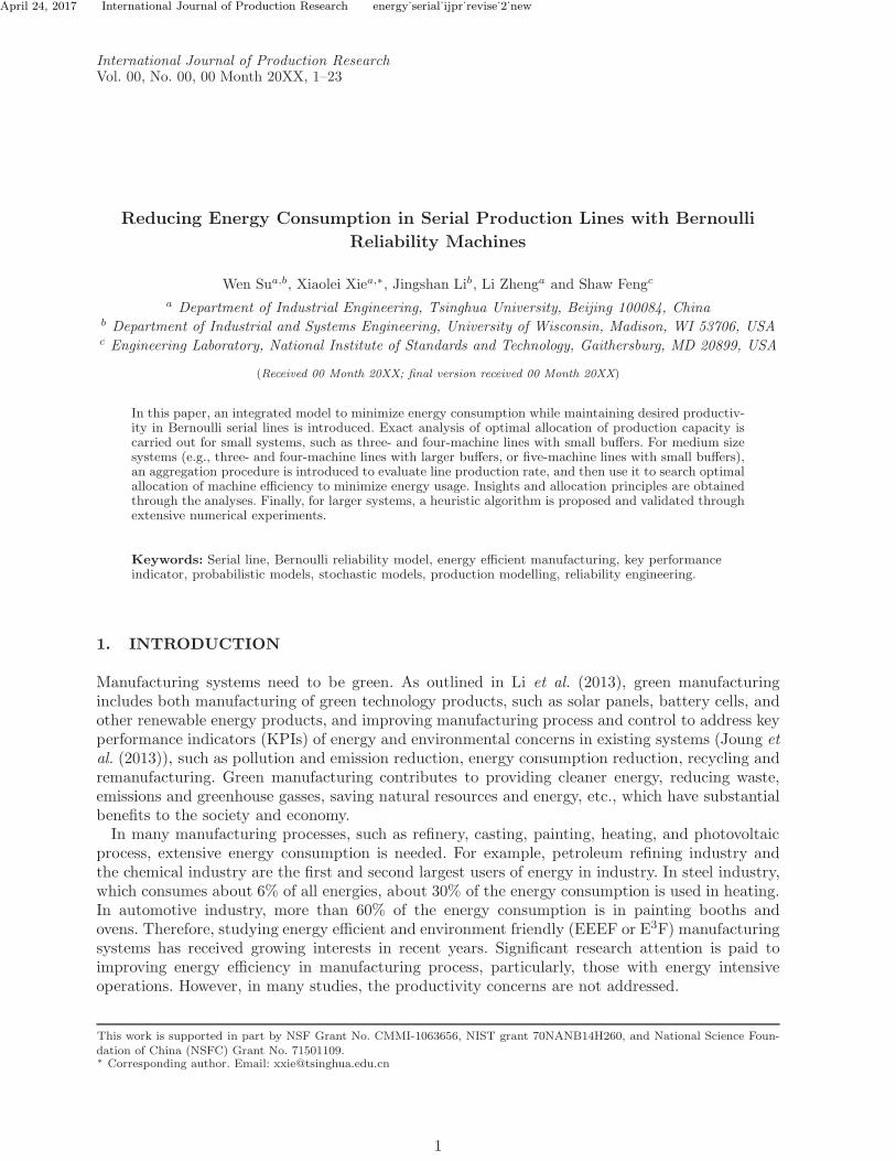
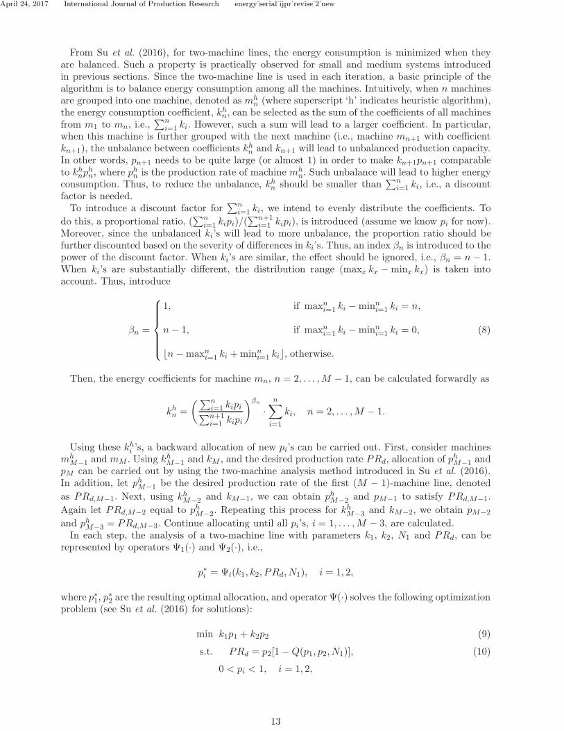
Consider a serial production line making one product type with M machines and M − 1 buffersseparating each pair of consecutive machines (see Figure 1 where the circles represent the machinesand the rectangles are the buffers). The following assumptions address the machines, the buffers,the energy consumption, and their mutual interactions.

2p1N1

p

m 1 b 1 m 2

NM-1 p M

b M-1 m M

Figure 1. Bernoulli serial line

(1) All machines have identical cycle time. During each cycle, machine mi, i = 1, . . . ,M , hasprobability pi to be up and 1−pi to be down. When a machine is up, it is capable of processinga part, while when it is down, no production takes place. The status of each machine isdetermined at the beginning of each cycle, independent of the status in the previous cycleand buffer contents.

(2) Buffer bi, i = 1, . . . ,M −1, has a finite capacity 0 ≤ Ni < ∞. The buffer status is determinedat the end of each cycle.

(3) If buffer bi, i = 1, . . . ,M − 1, is empty at the beginning of a cycle, then machine mi+1 isstarved in this time slot if it is up. Machine m1 is never starved.

(4) If buffer bi, i = 1, . . . ,M − 1, is full and machine mi+1 does not take a part from bi at thebeginning of a time slot, then machine mi is blocked during this cycle if it is up. MachinemM is never blocked.

(5) The energy consumption of machine mi, i = 1, . . . ,M , includes the average electrical powerto start up and maintain the machine and environment, and the power used to process theparts, kipi, which is proportional to its production capacity pi and ki is a constant, referredto as energy consumption coefficient.

(6) The desired production rate the system needs to maintain is denoted as PRd.

Remark 3.1. Bernoulli machine reliability model is assumed in this work. Such a model is typicallysuitable for assembly type systems where machine downtime is comparable to its cycle time. Forother systems, a transformation can be introduced that

pi =ci

cmax

·µi

λi + µi

,

where ci is speed (or capacity) of machine mi, and cmax = maxi ci. The shortest processing time(1/cmax) is selected as the unit for cycle time. In addition, λi and µi are the failure and repairrates of mi, respectively. Thus, parameter pi represents the probability to produce a part duringcycle time 1/cmax, and it can also be viewed as the relative efficiency or capacity of the machine,or the proportion of time the machine is working during a cycle. The Bernoulli model has beenused in many manufacturing system studies successfully (see monograph by Li and Meerkov (2009)and papers by Lim et al. (1990); Kuo et al. (1996); Li and Meerkov (2001); Arinez et al. (2010);Wang and Li (2010); Zhao and Li (2014)). In future work, other machine reliability models will bestudied.

Remark 3.2. In this study, we assume electrical power being the practical form of energy con-sidered. Such energy can be divided into two categories. One is the energy to start up and keepthe machine at an “on” or “ready” status as well as maintain the necessary environment (such astemperature, humidity, lights), which often require a fixed power. Another is the energy to operatethe machine to produce a part, which typically consumes power proportional to the machine’sprocessing rate (e.g., parameter pi). In this study, we focus on the second one. Thus, the energy

4


consumption for machine mi during a cycle is

Ei = kipi, i = 1, . . . ,M. (1)

Similar formulation is also given in Calvanese (2013), Gutowski et al. (2009) and Su et al. (2016).

Then the total energy consumed in a multi-machine line is

E =

M∑

i=1

kipi. (2)

The objective of this study is to seek the optimal allocation of machine capacity (or efficiency),

denoted as p∗i ’s, i = 1, . . . ,M , to minimize energy consumption E (or equivalently,∑M

i=1 kipi) whileensuring the desired production rate PRd. Define PR as the production rate of the serial line. Thenthe problem to be addressed can be formulated as:

min E =

M∑

i=1

kipi, (3)

s.t. PR ≥ PRd. (4)

Remark 3.3. In general, the failure rates (λi in Remark 3.1) may not be fully controllable butpredictable or observable. The repair rates (µi in Remark 3.1) are relatively easier to adjust and thespeed can be controlled. For example, many machines have some freedom to adjust the processingtime (1/ci), such as in machining and painting. In this case, it is still possible to control machineparameters to reach the desired pi. This has been achieved in many case studies (e.g., see Li andMeerkov (2009)).

To solve this problem, we first study three- and four-machine production lines with very smallbuffers to derive exact solutions. Then, for medium size systems (typical three- or four-machinelines with relatively large buffers), an aggregation procedure is introduced for production rateevaluation and then used for optimal solution search. Finally, for larger systems with five or moremachines, a heuristic algorithm is developed.

4. EXACT ANALYSIS FOR SMALL SYSTEMS

For small systems, it is possible to develop Markov chain models to derive exact results. In an appro-priately defined state space, transition probabilities can be defined, and steady state probabilitiescan be calculated by solving balance equations. Then the line production rate can be evaluated.By searching the possible scenarios, the optimal solution to minimize energy consumption whilemaintaining the desired production rate can be obtained.In this section, first, we analyze balanced lines with identical Ni’s, i = 1, . . . ,M − 1, and ki’s,

i = 1, . . . ,M . Next, lines with unequal Ni’s but equal ki’s are studied. Finally, systems withnonequal ki’s are investigated.

4.1 Lines with Identical Buffers and Energy Coefficients

First, consider the simplest three-machine line L1, where energy coefficients and buffer capacitiesare assumed to be one.

L1 : N1 = N2 = 1, k1 : k2 : k3 = 1 : 1 : 1.

5


According to Li and Meerkov (2009), the states of a Bernoulli production line can be rep-resented by the occupancy of the buffers. Thus, the state space of L1 can be described byS = {(0, 0), (1, 0), (0, 1), (1, 1)}. Let Pj,i be the transition probability from state j to state i, and Pi

be the steady state probability. Then the corresponding transition probability matrix and balanceequations can be obtained. Solving them we obtain:

Proposition 4.1. Under assumptions 1)-6), the steady state probabilities of Line L1 are

P(0,0) =(1− p1)

2p2p23

Λ, P(1,0) =

p1p3(p3 + p1(1− p2 − p3))

Λ,

P(0,1) =(1− p1)p1p2p3

Λ, P(1,1) =

p21p2Λ

, (5)

where

Λ = p21p2(1− p3)2 + p21p3(1− p3) + p2p

23 + p1p3(p2 + p3 − 2p2p3). (6)

Then the line production rate can be calculated as

PRL1 = (P(0,1) + P(1,1))p3 =(1− p1)p1p2p

23 + p21p2p3

Λ. (7)

Proof: See Appendix A.

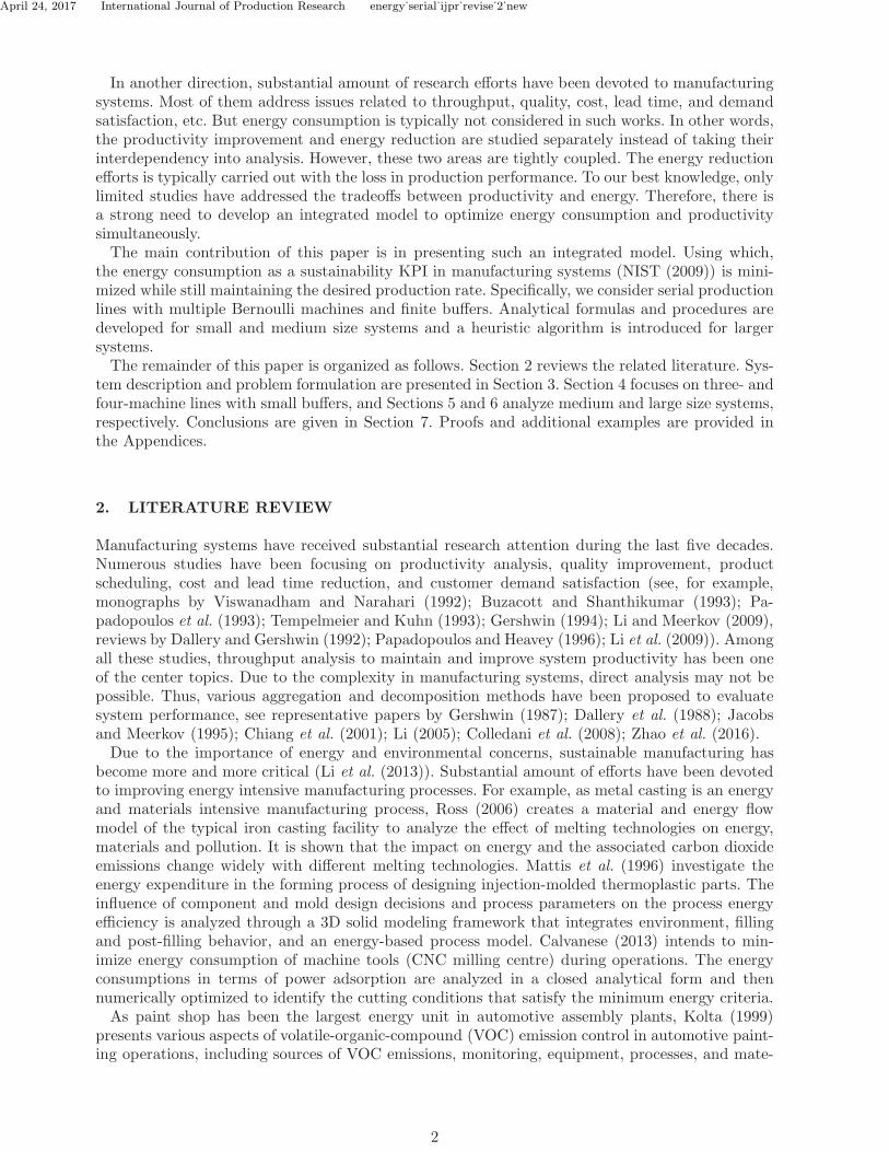
Although a closed-form expression of line production rate can be obtained, finding a closed-form solution of p∗i ’s, i = 1, 2, 3 for optimization problem (3) and (4) is impossible. Therefore,Mathematica is used to search the optimal p∗i ’s satisfying the desired production rate. The resultsare illustrated in Figure 2(a).

(a) L1 (b) L2

Figure 2. Optimal p∗i’s in L1 and L2

Similar analysis is applied to another three-machine line L2 with the only difference that allbuffer capacities are increased by 1, and the optimal allocations of pi’s are shown in Figure 2(b).

L2 : N1 = N2 = 2, k1 : k2 : k3 = 1 : 1 : 1.

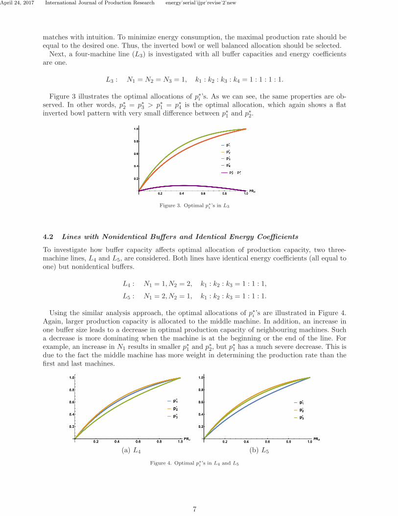
For both lines, p∗1 and p∗3 are always equal and smaller than p∗2, indicating that there exists aninverted bowl pattern for the optimal allocation of production capacity. In addition, the differencebetween p∗1 (or p∗3) and p∗2 is typically small, less than 0.05, and is also distributed as an invertedbowl shape with respect to PRd. Such small difference between p∗1 and p∗2 suggests that by evenlydistributing pi along the line, the result could be close to the optimal solution. Since the invertedbowl shape allocation delivers the maximal production rate and the performance difference betweeninverted bowl and evenly distributed allocations is very small (Li and Meerkov (2009)), such a result

6


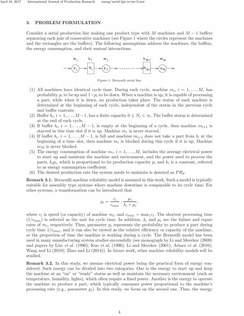
matches with intuition. To minimize energy consumption, the maximal production rate should beequal to the desired one. Thus, the inverted bowl or well balanced allocation should be selected.Next, a four-machine line (L3) is investigated with all buffer capacities and energy coefficients

are one.

L3 : N1 = N2 = N3 = 1, k1 : k2 : k3 : k4 = 1 : 1 : 1 : 1.

Figure 3 illustrates the optimal allocations of p∗i ’s. As we can see, the same properties are ob-served. In other words, p∗2 = p∗3 > p∗1 = p∗4 is the optimal allocation, which again shows a flatinverted bowl pattern with very small difference between p∗1 and p∗2.

Figure 3. Optimal p∗i’s in L3

4.2 Lines with Nonidentical Buffers and Identical Energy Coefficients

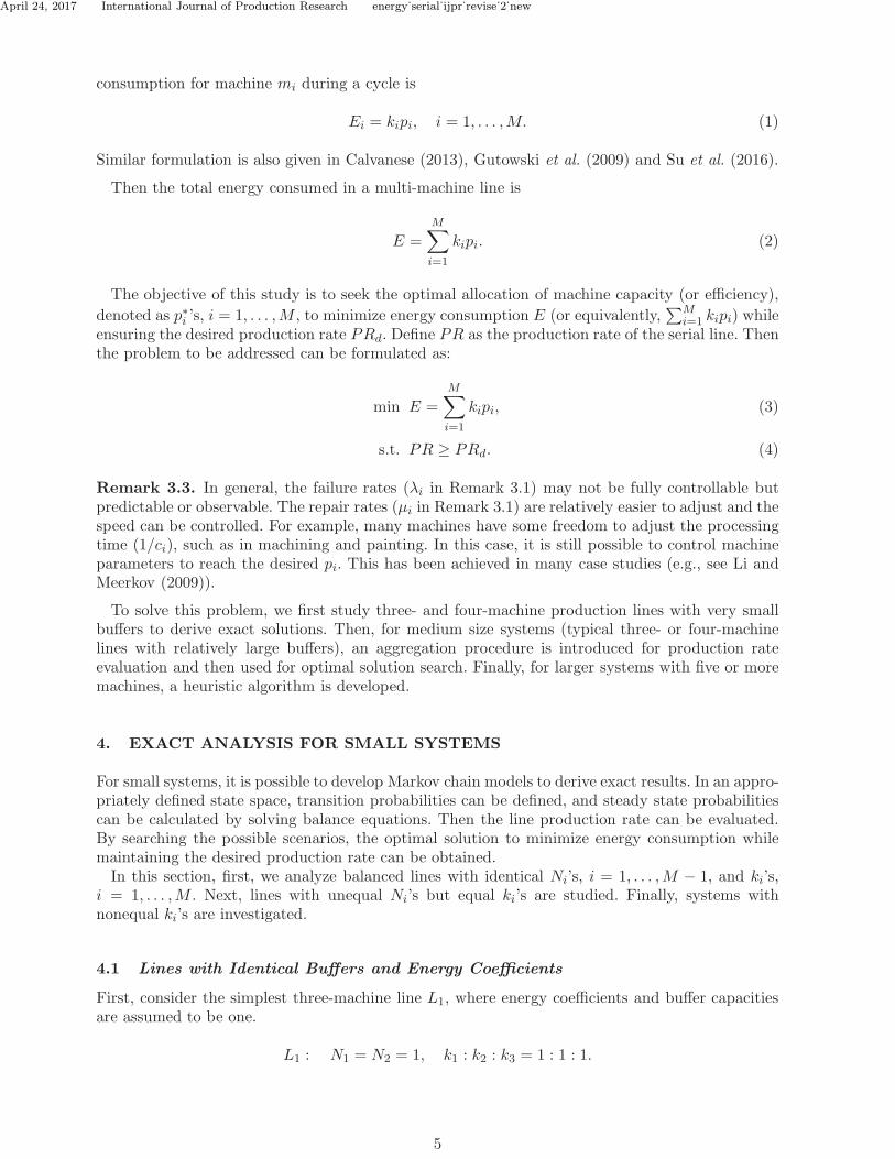
To investigate how buffer capacity affects optimal allocation of production capacity, two three-machine lines, L4 and L5, are considered. Both lines have identical energy coefficients (all equal toone) but nonidentical buffers.

L4 : N1 = 1, N2 = 2, k1 : k2 : k3 = 1 : 1 : 1,

L5 : N1 = 2, N2 = 1, k1 : k2 : k3 = 1 : 1 : 1.

Using the similar analysis approach, the optimal allocations of p∗i ’s are illustrated in Figure 4.Again, larger production capacity is allocated to the middle machine. In addition, an increase inone buffer size leads to a decrease in optimal production capacity of neighbouring machines. Sucha decrease is more dominating when the machine is at the beginning or the end of the line. Forexample, an increase in N1 results in smaller p∗1 and p∗2, but p

∗

1 has a much severe decrease. This isdue to the fact the middle machine has more weight in determining the production rate than thefirst and last machines.

(a) L4 (b) L5


7


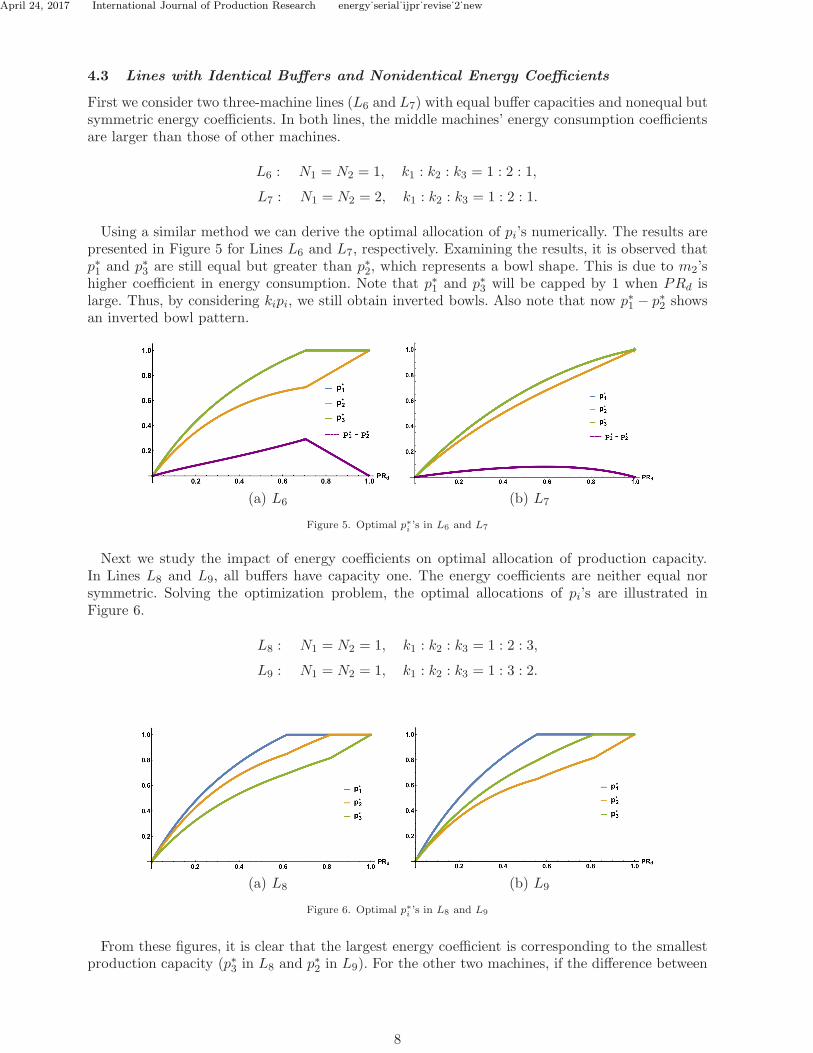
4.3 Lines with Identical Buffers and Nonidentical Energy Coefficients

First we consider two three-machine lines (L6 and L7) with equal buffer capacities and nonequal butsymmetric energy coefficients. In both lines, the middle machines’ energy consumption coefficientsare larger than those of other machines.

L6 : N1 = N2 = 1, k1 : k2 : k3 = 1 : 2 : 1,

L7 : N1 = N2 = 2, k1 : k2 : k3 = 1 : 2 : 1.

Using a similar method we can derive the optimal allocation of pi’s numerically. The results arepresented in Figure 5 for Lines L6 and L7, respectively. Examining the results, it is observed thatp∗1 and p∗3 are still equal but greater than p∗2, which represents a bowl shape. This is due to m2’shigher coefficient in energy consumption. Note that p∗1 and p∗3 will be capped by 1 when PRd islarge. Thus, by considering kipi, we still obtain inverted bowls. Also note that now p∗1 − p∗2 showsan inverted bowl pattern.

(a) L6 (b) L7


Next we study the impact of energy coefficients on optimal allocation of production capacity.In Lines L8 and L9, all buffers have capacity one. The energy coefficients are neither equal norsymmetric. Solving the optimization problem, the optimal allocations of pi’s are illustrated inFigure 6.

L8 : N1 = N2 = 1, k1 : k2 : k3 = 1 : 2 : 3,

L9 : N1 = N2 = 1, k1 : k2 : k3 = 1 : 3 : 2.

(a) L8 (b) L9


From these figures, it is clear that the largest energy coefficient is corresponding to the smallestproduction capacity (p∗3 in L8 and p∗2 in L9). For the other two machines, if the difference between

8


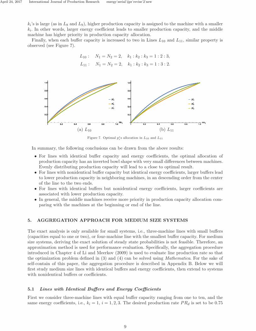
ki’s is large (as in L8 and L9), higher production capacity is assigned to the machine with a smallerki. In other words, larger energy coefficient leads to smaller production capacity, and the middlemachine has higher priority in production capacity allocation.Finally, when each buffer capacity is increased to two in Lines L10 and L11, similar property is

observed (see Figure 7).

L10 : N1 = N2 = 2, k1 : k2 : k3 = 1 : 2 : 3,

L11 : N1 = N2 = 2, k1 : k2 : k3 = 1 : 3 : 2.

(a) L10 (b) L11

Figure 7. Optimal p∗is allocation in L10 and L11

In summary, the following conclusions can be drawn from the above results:

• For lines with identical buffer capacity and energy coefficients, the optimal allocation ofproduction capacity has an inverted bowl shape with very small differences between machines.Evenly distributing production capacity will lead to a close to optimal result.

• For lines with nonidentical buffer capacity but identical energy coefficients, larger buffers leadto lower production capacity in neighboring machines, in an descending order from the centerof the line to the two ends.

• For lines with identical buffers but nonidentical energy coefficients, larger coefficients areassociated with lower production capacity.

• In general, the middle machines receive more priority in production capacity allocation com-paring with the machines at the beginning or end of the line.

5. AGGREGATION APPROACH FOR MEDIUM SIZE SYSTEMS

The exact analysis is only available for small systems, i.e., three-machine lines with small buffers(capacities equal to one or two), or four-machine line with the smallest buffer capacity. For mediumsize systems, deriving the exact solution of steady state probabilities is not feasible. Therefore, anapproximation method is used for performance evaluation. Specifically, the aggregation procedureintroduced in Chapter 4 of Li and Meerkov (2009) is used to evaluate line production rate so thatthe optimization problem defined in (3) and (4) can be solved using Mathematica. For the sake ofself-contain of this paper, the aggregation procedure is described in Appendix B. Below we willfirst study medium size lines with identical buffers and energy coefficients, then extend to systemswith nonidentical buffers or coefficients.

5.1 Lines with Identical Buffers and Energy Coefficients

First we consider three-machine lines with equal buffer capacity ranging from one to ten, and thesame energy coefficients, i.e., ki = 1, i = 1, 2, 3. The desired production rate PRd is set to be 0.75

9


(and in all subsequent studies).As one can see from Table 1, larger buffer size always implies smaller production capacity allo-

cation for each machine, resulting in lower energy consumption. The rationale behind this is thatlarger buffers lead to higher production rate. Thus, to only maintain the desired production rate,machine reliability can be reduced so that the required energy consumption will be smaller. In ad-dition, Table 1 suggests that the production capacity is almost evenly distributed, which is slightlydifferent with the results obtained for small buffer systems in the previous section (such as theinverted bowl shape). However, the difference is small. In the first two rows of Table 1, comparisonwith the optimal results obtained through exact analysis is provided. Clearly, the differences aresmaller than 0.8%, which indicates that the results obtained using aggregation procedure provideclose to optimal solutions of allocating p∗i ’s. Such differences are in the same order as throughputdifference between an inverted bowl allocation and a well balanced distribution (see Li and Meerkov(2009)). Note that for other rows and in subsequent tables, exact analysis cannot generate optimalresults due to high dimension of transition matrices, thus an “N/A” note is presented.

Table 1. Three-machine lines with identical buffers and energy coefficients (ki = 1, i = 1, 2, 3)

N1, N2 p∗1, p∗

2, p∗

3

∑ikip

∗

iComparison

1, 1 0.900, 0.900, 0.900 2.700 0.4%

2, 2 0.852, 0.850, 0.850 2.552 0.8%

3, 3 0.827, 0.825, 0.825 2.476 N/A

4, 4 0.811, 0.810, 0.810 2.431 N/A

5, 5 0.801, 0.800, 0.800 2.400 N/A

6, 6 0.794, 0.793, 0.793 2.379 N/A

7, 7 0.788, 0.787, 0.787 2.362 N/A

8, 8 0.784, 0.783, 0.783 2.350 N/A

9, 9 0.780, 0.780, 0.780 2.340 N/A

10, 10 0.778, 0.777, 0.777 2.332 N/A

For four-machine lines with identical buffers (capacities one to three) and energy coefficients,similar results can be observed (as shown in Table 2). Again the first row in Table 2 shows thecomparison with the optimal solution, and the difference is only 0.7%.

Table 2. Four-machine lines with identical buffers and energy coefficients (ki = 1, i = 1, . . . , 4)

N1, N2, N3 p∗1, p∗

2, p∗

3, p∗

4

∑ikip

∗

iComparison

1, 1, 1 0.923, 0.923, 0.923, 0.923 3.692 0.7%

2, 2, 2 0.873, 0.871, 0.896, 0.896 3.483 N/A

3, 3, 3 0.843, 0.842, 0.840, 0.840 3.367 N/A

Similar results are obtained for five-machine lines with small buffer capacities (one or two, seeTable 3). Note that in this case, exact analysis is unavailable.

Table 3. Five-machine lines with identical buffers and energy coefficients (ki = 1, i = 1, . . . , 5)

N1, N2, N3, N4 p∗1, p∗

2, p∗

3, p∗

4, p∗

5

∑ikip

∗

i

1,1,1,1 0.938, 0.938, 0.938, 0.938, 0.938 4.689

2,2,2,2 0.887, 0.886, 0.884, 0.883, 0.883 4.423

Therefore, we conclude that for lines with identical buffers and energy coefficients, evenly dis-tributing production capacity is a practical way to minimize energy usage and maintain the desiredproductivity level.

10


5.2 Lines with Nonidentical Buffers and Equal Energy Coefficients

To study the impact of buffer capacity, we consider three- and four-machine lines with differentbuffer capacities but equal energy coefficients, and results are presented in Tables 4 and 5, respec-tively.

Table 4. Three-machine lines with nonidentical buffers and equal energy coefficients

N1, N2 p∗1, p∗

2, p∗

3

∑ikip

∗

iComparison

1, 2 0.964, 0.835, 0.835 2.634 1.0%

2, 1 0.834, 0.891, 0.891 2.617 0.3%

2, 3 0.859, 0.830, 0.830 2.521 N/A

3, 2 0.822, 0.843, 0.843 2.509 N/A

2, 4 0.863, 0.820, 0.820 2.502 N/A

4, 2 0.806, 0.839, 0.839 2.484 N/A

Table 5. Four-machine lines with nonidentical buffers and equal energy coefficients

N1, N2, N3 p∗1, p∗

2, p∗

3, p∗

4

∑ikip

∗

i

2, 1, 1 0.840, 0.923, 0.923, 0.923 3.608

1, 2, 1 0.994, 0.834, 0.892, 0.892 3.617

1, 1, 2 0.974, 0.974, 0.843, 0.843 3.633

2, 2, 3 0.878, 0.876, 0.850, 0.850 3.454

3, 2, 2 0.836, 0.868, 0.866, 0.866 3.434

2, 3, 2 0.880, 0.842, 0.861, 0.861 3.444

3, 3, 4 0.845, 0.844, 0.830, 0.830 3.350

3, 4, 3 0.846, 0.825, 0.836, 0.836 3.343

4, 3, 3 0.822, 0.840, 0.838, 0.838 3.339

Again as one can see, in Table 4, an increase in N1 leads to decreases in p∗1, and sometimes p∗2as well. Similarly, larger N2 also indicates smaller p∗2 and p∗3. Energy is reduced in both cases. InTable 5, an N3’s increase implies decreases in p∗1 and p∗2. Thus, the conclusions are consistent, i.e.,an increase in Ni leads to decreases in p∗i and possible p∗i+1 as well as the total energy consumed.Comparing to exact analysis, the results from aggregation-based method only have small differences(within 1.0%, see the first two rows in Table 4). The properties obtained from exact analysis stillapply.For five-machine lines with small buffers, as before, similar properties are observed (Table 6).

Table 6. Five-machine lines with nonidentical buffers and equal energy coefficients

N1, N2, N3, N4 p∗1, p∗

2, p∗

3, p∗

4, p∗

5

∑ikip

∗

i

2, 3, 2, 2 0.893, 0.850, 0.880, 0.879, 0.879 4.380

2, 2, 3, 2 0.892, 0.891, 0.855, 0.874, 0.874 4.302

5.3 Lines with Identical Buffers and Unbalanced Energy Coefficients

To investigate the impact of energy consumption coefficients, lines with nonidentical energy coef-ficients are considered. In Table 7, three-machine lines with identical buffers (N1 = N2 = 2) butdifferent energy coefficients are studied. Four different patterns of ki’s are considered: ramp, slope,bowl-type, and inverted bowl-type. As one can observe, an increasing (or decreasing) pattern of en-ergy coefficients results in a decreasing (respectively, increasing) distribution of optimal productioncapacity. In bowl and inverted bowl shapes of ki’s allocation, p∗i ’s follow an inverted bowl and aregular bowl pattern, respectively. In addition, comparing with the exact solutions, the allocationsusing the aggregation procedure lead to close to optimal results, with differences less than 1.5%.

11


Table 7. Three-machine lines with identical buffers (N1 = N2 = 2) but different energy coefficients

k1 : k2 : k3 p∗1, p∗

2, p∗

3

∑ikip

∗

iComparison

1 : 1.2 : 1.5 0.878, 0.855, 0.824 3.141 0.8%

1 : 2 : 3 0.926, 0.856, 0.800 5.040 0.5%

3 : 2 : 1 0.800, 0.856, 0.928 5.041 0.5%

2 : 1 : 2 0.830, 0.910, 0.828 4.227 1.4%

1 : 2 : 1 0.889, 0.797, 0.888 3.371 0.3%

When four-machine lines are considered, similar properties still follow, as illustrated in Table 8.This is also true for the five-machine case (see Table 9). In addition, note that the significantlyhigher energy consumptions in the first two rows of Tables 8 and 9 than those in other lines aredue to much larger energy coefficients. Thus, we still claim that in lines with identical buffers, theproduction capacity needs to be allocated negatively to the energy coefficients distribution.

Table 8. Four-machine lines with identical buffers (Ni = 2, i = 1, 2, 3) but different energy coefficients

k1 : k2 : k3 : k4 p∗1, p∗

2, p∗

3, p∗

4

∑ikip

∗

i

1 : 2 : 3 : 4 0.951, 0.902, 0.856, 0.816 8.587

4 : 3 : 2 : 1 0.818, 0.855, 0.900, 0.955 8.594

1 : 2 : 1 : 2 0.916, 0.839, 0.916, 0.837 5.184

2 : 1 : 1 : 2 0.840, 0.916, 0.916, 0.836 5.184

1 : 2 : 2 : 1 0.916, 0.839, 0.837, 0.916 5.184

Table 9. Five-machine lines with identical buffers (Ni = 2, i = 1, 2, 3, 4) but different energy coefficients

k1 : k2 : k3 : k4 : k5 p∗1, p∗

2, p∗

3, p∗

4, p∗

5

∑ikip

∗

i

1 : 1.5 : 2 : 2.5 : 3 0.945, 0.917, 0.890, 0.863, 0.839 8.774

3 : 2.5 : 2 : 1.5 : 1 0.842, 0.864, 0.888, 0.916, 0.947 8.782

1 : 2 : 1 : 2 : 1 0.921, 0.847, 0.921, 0.844, 0.920 6.145

1 : 2 : 2 : 2 : 1 0.931, 0.864, 0.862, 0.860, 0.931 7.034

2 : 1 : 1 : 1 : 2 0.848, 0.921, 0.921, 0.920, 0.843 6.146

The above results indicate that, for medium size systems, the method based on aggregation pro-cedure can be applied to search the optimal production capacity allocations for energy consumptionminimization while still ensuring the desired line throughput. When systems become more complex,the search space for optimal solution becomes too large so that computation intensity becomes anissue. Thus, a heuristic method will be pursued.

6. HEURISTIC METHOD FOR LARGE SYSTEMS

Although the aggregation approach can be used to study medium size systems, computation in-tensity still limits its application to larger systems. Therefore, in this section, a heuristic methodis proposed for systems with more than five machines. First, a heuristic algorithm is introduced.Then, the performance of the algorithm is studied by comparing with the results from aggregationapproach in medium size systems, and with simulation results in larger systems.

6.1 Algorithm Description

The idea of the heuristic algorithm is to forwardly group the energy consumption coefficients oftwo machines into one, and continue until the last one, then backwardly derive production capacityallocation for every two machines until the first one. Such a process is repeated until convergenceand the energy efficiency can be improved while still maintaining the desired production rate.

12


From Su et al. (2016), for two-machine lines, the energy consumption is minimized when theyare balanced. Such a property is practically observed for small and medium systems introducedin previous sections. Since the two-machine line is used in each iteration, a basic principle of thealgorithm is to balance energy consumption among all the machines. Intuitively, when n machinesare grouped into one machine, denoted as mh

n (where superscript ‘h’ indicates heuristic algorithm),the energy consumption coefficient, khn, can be selected as the sum of the coefficients of all machinesfrom m1 to mn, i.e.,

∑ni=1 ki. However, such a sum will lead to a larger coefficient. In particular,

when this machine is further grouped with the next machine (i.e., machine mn+1 with coefficientkn+1), the unbalance between coefficients khn and kn+1 will lead to unbalanced production capacity.In other words, pn+1 needs to be quite large (or almost 1) in order to make kn+1pn+1 comparableto khnp

hn, where p

hn is the production rate of machine mh

n. Such unbalance will lead to higher energyconsumption. Thus, to reduce the unbalance, khn should be smaller than

∑ni=1 ki, i.e., a discount

factor is needed.To introduce a discount factor for

∑ni=1 ki, we intend to evenly distribute the coefficients. To

do this, a proportional ratio, (∑n

i=1 kipi)/(∑n+1

i=1 kipi), is introduced (assume we know pi for now).Moreover, since the unbalanced ki’s will lead to more unbalance, the proportion ratio should befurther discounted based on the severity of differences in ki’s. Thus, an index βn is introduced to thepower of the discount factor. When ki’s are similar, the effect should be ignored, i.e., βn = n− 1.When ki’s are substantially different, the distribution range (maxx kx −minx kx) is taken intoaccount. Thus, introduce

βn =

1, if maxni=1 ki −minni=1 ki = n,

n− 1, if maxni=1 ki −minni=1 ki = 0,

⌊n−maxni=1 ki +minni=1 ki⌋, otherwise.

(8)

Then, the energy coefficients for machine mn, n = 2, . . . ,M − 1, can be calculated forwardly as

khn =

(∑ni=1 kipi

∑n+1i=1 kipi

)βn

·

n∑

i=1

ki, n = 2, . . . ,M − 1.

Using these khi ’s, a backward allocation of new pi’s can be carried out. First, consider machinesmh

M−1 and mM . Using khM−1 and kM , and the desired production rate PRd, allocation of phM−1 andpM can be carried out by using the two-machine analysis method introduced in Su et al. (2016).In addition, let phM−1 be the desired production rate of the first (M − 1)-machine line, denoted

as PRd,M−1. Next, using khM−2 and kM−1, we can obtain phM−2 and pM−1 to satisfy PRd,M−1.

Again let PRd,M−2 equal to phM−2. Repeating this process for khM−3 and kM−2, we obtain pM−2

and phM−3 = PRd,M−3. Continue allocating until all pi’s, i = 1, . . . ,M − 3, are calculated.In each step, the analysis of a two-machine line with parameters k1, k2, N1 and PRd, can be

represented by operators Ψ1(·) and Ψ2(·), i.e.,

p∗i = Ψi(k1, k2, PRd, N1), i = 1, 2,

where p∗1, p∗

2 are the resulting optimal allocation, and operator Ψ(·) solves the following optimizationproblem (see Su et al. (2016) for solutions):

min k1p1 + k2p2 (9)

s.t. PRd = p2[1−Q(p1, p2, N1)], (10)

0 < pi < 1, i = 1, 2,

13


where

Q(x, y,N) =

(1− x)(1− α(x, y))

1− xyαN (x, y)

, if x 6= y,

1− x

N + 1− y, if x = y,

(11)

α(x, y) =x(1− y)

y(1− x). (12)

6.2 Recursive Procedure

Since the above algorithm relies on values of pi that are unknown, we introduce iterations tocontinuously update pi during each iteration. Formally, let khi (j) and phi (j) denote the energyconsumption coefficient and the production capacity allocation for machine mh

i during iterationj, respectively. Also denote pi(j) as the production capacity for machine mi, and PRd,i(j) be thedesired production rate for machines m1 to mi, during iteration j. Then, the recursive procedurecan be formally expressed as:

Procedure 6.1. Step 1: Initialization.

khn(0) =

(∑ni=1 ki

∑n+1i=1 ki

)βn

·

n∑

i=1

ki, n = 2, . . . ,M − 1,

pi(0) = 1, i = 1, . . . ,M,

kh1 (j) = k1, ∀j, (13)

PRd,M (j) = PRd, ∀j.

Let iteration number j = 1.Step 2: Forward calculation of energy consumption coefficients.

khn(j) =

(∑ni=1 kipi(j − 1)

∑n+1i=1 kipi(j − 1)

)βn

·

n∑

i=1

ki, n = 2, . . . ,M − 1. (14)

Step 3: Backward allocation of production capacity. For i = M, . . . , 2,

phi−1(j) = Ψ1(khi−1(j − 1), ki, PRd,i(j), Ni−1),

pi(j) = Ψ2(khi−1(j − 1), ki, PRd,i(j), Ni−1), (15)

PRd,i−1(j) = phi−1(j).

Step 4: Check iteration stop condition. For j ≤ 100, if

maxi

|pi(j)− pi(j − 1)| < ∆1,

where ∆1 is typically set to 10−7, then go to Step 5, otherwise, let j = j + 1, and go back to Step

14


2. For j > 100, let

khn(j + 2) =khn(j + 1) + khn(j)

2. (16)

Then go back to Step 2.Step 5: Check desired production rate. If

PR− PRd < ∆2,

where ∆2 is typically selected as 10−5, then stop the procedure and assign pi(j) to p∗i , i = 2, . . . ,M ,and ph1(j) to p∗1. Otherwise

pi(j) = pi(j)− 0.001, i = 2, . . . ,M,

ph1(j) = ph1(j) − 0.001,

and repeat Step 5.

6.3 Convergence

To study the convergence of Procedure 6.1, we first investigate the bounds between iterations. Forconvenience, define

δn(j) = |khn(j)− khn(j − 1)|, j = 1, 2, . . . . (17)

In addition, let

B1(n) =

(

1

1 + 1PRd

kn+1∑n

i=1ki

)βn

·

n∑

i=1

ki,

B2(n) =

(

1

1 + PRdkn+1∑n

i=1ki

)βn

·

n∑

i=1

ki. (18)

Then we obtain bounds for khn during each iteration.

Proposition 6.1. Under assumptions 1)-6), both khn(j) and δn(j) in Procedure 6.1 are bounded,i.e.,

khn(j) ∈

(B1(n), B2(n)), if βn > 0,

(B2(n), B1(n)), if βn < 0,

δn(j) ∈ [0, |B1(n)−B2(n)|). (19)


Moreover, for three-machine lines, δn(j) converges to δn when j is large. Then δn is not onlybounded, but also unique.

Proposition 6.2. Under assumptions 1)-6) with M = 3, if 0 ≪ PRd < 1, then δn in Procedure6.1 is unique.

15



The results of Proposition 6.2 indicate that khn(j) is either oscillating with a small bound orconverging. Similar observations are discovered for longer lines. To verify the convergence of theprocedure, thousands of experiments are carried out. In all cases, the convergence of the procedureis observed. Thus we formulate it as a numerical observation.

Numerical Observation 1. Under assumptions 1)-6), Procedure 6.1 converges, i.e., the fol-lowing limits exist

limj→∞

pi(j) := p∗i , i = 2, . . . ,M, (20)

limj→∞

ph1(j) := p∗1. (21)

Remark 6.1. Among over 10,000 experiments with randomly selected parameters, except two orthree, Procedure 6.1 converges within 10 iterations. For the two or three exceptions, the differencebetween khi (j) and khi (j+1) is around 0.001 after 100 iterations. Then the adjustment (16) in Step4 makes the procedure converges immediately.

6.4 Accuracy

To investigate the accuracy of Procedure 6.1, numerical experiments are carried out to comparethe results from Procedure 6.1 with the “optimal” solutions. For three- to five-machine lines, the“optimal” solutions are obtained using the aggregation approach introduced in Section 5. Therelative differences are defined as

ǫ =(∑

kip∗

i )h − (

∑

kip∗

i )a

(∑

kip∗

i )a

· 100%,

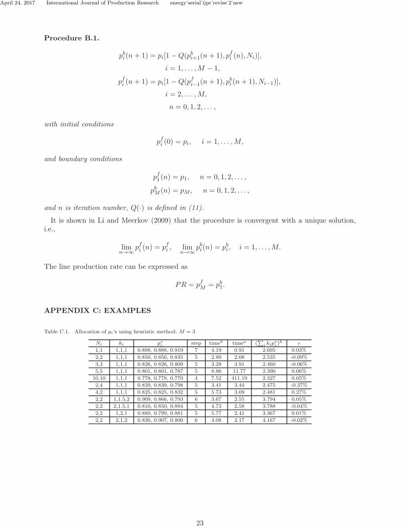
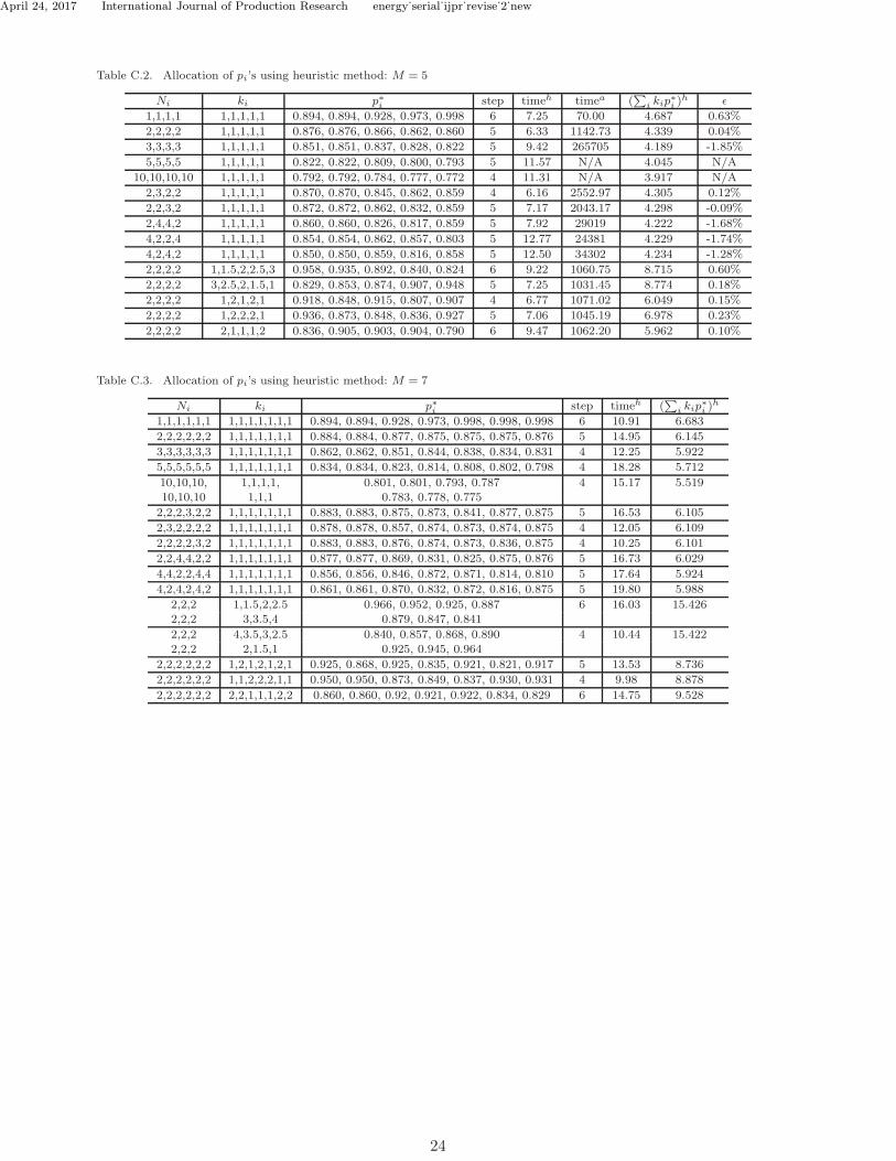
where superscripts “h” and “a” denote heuristic method and aggregation approach, respectively.As shown in Tables C.1 and C.2 in Appendix C for three- and five-machine lines, in most cases

the differences are within 0.1% and the largest ones are still less than 1%. In addition, the iterationsteps are also included in these tables, as well as the computation time using the two methods. Asone can see, when the system is small, aggregation approach is faster; while when buffers becomelarge, heuristic method is more efficient. Again note that two examples in Table C.2 with largebuffers do not have aggregation results due to computation intensity, thus are marked with “N/A”.For six- to ten-machine systems, Monte Carlo simulations are introduced to generate numerous

feasible solutions. 5000 lines are randomly generated using the following parameter ranges:

M ∈ [6, 10],

PRd ∈ [0.6, 0.95],

Ni ∈ [1, 10],

ki ∈ [1, 10].

Tables C.3 and C.4 in Appendix C illustrate the examples of such experiments for seven- andten-machine lines. Thousands of experiments are carried out by randomly generating pi’s until thedesired production rate is satisfied. Then the one with the smallest

∑

i kipi is considered as the“optimal” one. By comparing the “optimal” solution with the one calculated by heuristic algorithm,we observe that only in 205 out of 5,000 examples (i.e., 4.10%) the “optimal” solution leads tosmaller amount of consumed energy comparing with the results from heuristic method. Among

16


the 205 cases, 70% of them have gaps within 1%, and 90% within 2%, while the maximum gap is5.73%.Therefore, we claim that Procedure 6.1 provides an optimal or a close to optimal solution of

allocating production capacity to minimize energy consumptions.

6.5 System Property

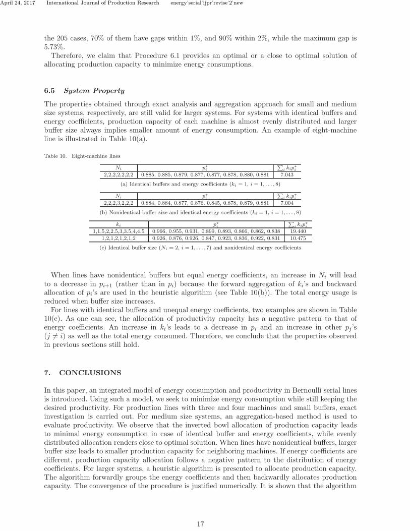
The properties obtained through exact analysis and aggregation approach for small and mediumsize systems, respectively, are still valid for larger systems. For systems with identical buffers andenergy coefficients, production capacity of each machine is almost evenly distributed and largerbuffer size always implies smaller amount of energy consumption. An example of eight-machineline is illustrated in Table 10(a).

Table 10. Eight-machine lines

Ni p∗i

∑ikip

∗

i

2,2,2,2,2,2,2 0.885, 0.885, 0.879, 0.877, 0.877, 0.878, 0.880, 0.881 7.043

(a) Identical buffers and energy coefficients (ki = 1, i = 1, . . . , 8)

Ni p∗i

∑ikip

∗

i

2,2,2,3,2,2,2 0.884, 0.884, 0.877, 0.876, 0.845, 0.878, 0.879, 0.881 7.004

(b) Nonidentical buffer size and identical energy coefficients (ki = 1, i = 1, . . . , 8)

ki p∗i

∑ikip

∗

i

1,1.5,2,2.5,3,3.5,4,4.5 0.966, 0.955, 0.931, 0.899, 0.893, 0.866, 0.862, 0.838 19.440

1,2,1,2,1,2,1,2 0.926, 0.876, 0.926, 0.847, 0.923, 0.836, 0.922, 0.831 10.475

(c) Identical buffer size (Ni = 2, i = 1, . . . , 7) and nonidentical energy coefficients

When lines have nonidentical buffers but equal energy coefficients, an increase in Ni will leadto a decrease in pi+1 (rather than in pi) because the forward aggregation of ki’s and backwardallocation of pi’s are used in the heuristic algorithm (see Table 10(b)). The total energy usage isreduced when buffer size increases.For lines with identical buffers and unequal energy coefficients, two examples are shown in Table

10(c). As one can see, the allocation of productivity capacity has a negative pattern to that ofenergy coefficients. An increase in ki’s leads to a decrease in pi and an increase in other pj’s(j 6= i) as well as the total energy consumed. Therefore, we conclude that the properties observedin previous sections still hold.

7. CONCLUSIONS

In this paper, an integrated model of energy consumption and productivity in Bernoulli serial linesis introduced. Using such a model, we seek to minimize energy consumption while still keeping thedesired productivity. For production lines with three and four machines and small buffers, exactinvestigation is carried out. For medium size systems, an aggregation-based method is used toevaluate productivity. We observe that the inverted bowl allocation of production capacity leadsto minimal energy consumption in case of identical buffer and energy coefficients, while evenlydistributed allocation renders close to optimal solution. When lines have nonidentical buffers, largerbuffer size leads to smaller production capacity for neighboring machines. If energy coefficients aredifferent, production capacity allocation follows a negative pattern to the distribution of energycoefficients. For larger systems, a heuristic algorithm is presented to allocate production capacity.The algorithm forwardly groups the energy coefficients and then backwardly allocates productioncapacity. The convergence of the procedure is justified numerically. It is shown that the algorithm

17


leads to an optimal or a close to optimal solution. The system properties obtained in small andmedium systems are still suitable for large systems.The results of this work provide production engineers a quantitative tool to effectively operate

the system to reduce energy consumption and meet production target. The future work can bedirected to the following areas:

• Extending the study to other machine reliability models, such as geometric, exponential, orgeneral reliability machines.

• Generalizing to flexible manufacturing systems that can produce multiple product types.• Investigating the continuous improvement strategies, such as identifying the energy bottleneck

machines, i.e., the machines whose reduction in energy coefficient will lead to the largestreduction in total energy consumption, and the energy bottleneck buffers, whose increasewill lead to the largest reduction in system energy.

• Applying the results on the factory floor to design and control the production line for energyefficiency.

References

Arinez, J., Biller, S., Meerkov, S.M. and Zhang, L., 2010. Quality/quantity improvement in an automotivepaint shop: a case study. IEEE Transactions on Automation Science and Engineering, 7 (4), 755–761.

Branham, M., 2008. Semiconductors and Sustainability: Energy and Materials Use in the Integrated CircuitIndustry. M.S. Thesis, Department of Mechanical Engineering, Massachusetts Institute of Technology,Cambridge, MA.

Buzacott, J.A. and Shanthikumar, J.G., 1993. Stochastic Models of Manfacturing Systems. Prentice Hall,Englewood Cliffs, NJ.

Calvanese, M.L., Albertelli, P., Matta, A. and Taisch, M. 2013. Analysis of energy consumption in CNCmachining centers and determination of optimal cutting conditions. Re-engineering Manufacturing forSustainability, Eds. Nee, A.Y.C., Song, B. and Ong, S.-K., 227–232.

Chiang, S.-Y., Kuo, C.-T. and Meerkov, S.M. 2001 c-Bottlenecks in serial production lines: identificationand application. Mathematical Problems in Engineering, 7 (6), 543–578.

Chen, G., Zhang, L., Arinez, J. and Biller, S., 2013. Energy-efficient production systems through schedule-based operations. IEEE Transactions on Automation Science and Engineering, 10 (1), 27–37.

Colledani, M., Gandola, F., Matta, A. and Tolio, T. 2008. Performance evaluation of linear and non-linearmulti-product multi-stage lines with unreliable machines and finite homogeneous buffers. IIE Transactions,40 (6), 612–626.

Dallery, Y., David, R. and Xie, X.L., 1988. An efficient algorithm for analysis of transfer lines with unreliablemachines and finite buffers. IIE transactions, 20 (3), 280–283.

Dallery, Y. and Gershwin, S.B., 1992. Manufacturing flow line systems: a review of models and analyticalresults. Queueing Systems: Theory and Applications, 12 (1), 3–94.

Fernandez, M., Li, L. and Sun, Z., 2011. Just-for-peak buffer inventory for peak electricity demand reductionof manufacturing systems. International Journal of Production Economics, 146, 178-184.

Frigerio, N. and Matta, A., 2015. Energy-efficient control strategies for machine tools with stochastic arrivals.IEEE Transactions on Automation Science and Engineering, 12 (1), 50–61.

Galitsky, C. and Worrell E. 2008. Energy efficiency improvement and cost saving opportunitiesfor the vehicle assembly industry. Lawrence Berkeley National Laboratory (LBNL-50939-Revision).http://www.energystar.gov/ia/business/industry/LBNL-50939.pdf. Accessed September 21, 2015.

Gershwin, S.B., 1987. An efficient decomposition method for the approximate evaluation of tandem queueswith finite storage space and blocking. Operations Research, 35 (2), 291–305.

Gershwin, S.B., 1994. Manufacturing Systems Engineering. Prentice Hall, Englewood Cliffs, NJ.Giret, A., Trentesaux, D. and Prabhu, V., 2015. Sustainability in manufacturing operations scheduling: A

state of the art review. Journal of Manufacturing Systems, 37 (1), 126–140.Guerrero, C.P.A., Wang, J., Li, J., Arinez, J., Biller, S., Huang, N. and Xiao, G., 2011. Production system

design to achieve energy savings in automotive paint shop. International Journal of Production Research,49, 6769–6785.

Gutowski, T.G., Branham, M.S., Dahmus, J.B., Jones, A.J., Thiriez, A. and D.P. Sekulic, 2009. Thermo-

18


dynamic analysis of resources used in manufacturing processes. Environmental Science & Technology, 43,1584–1590.

Gyftopoulos, E.P. and Beretta, G.P., 2005. Thermodynamics: Foundations and Applications. Dover Publi-cations, New York, NY.

Jacobs, D. and Meerkov, S.M., 1995. A system-theoretic property of serial production lines: improvability.International Journal of Systems Science, 26 (4), 755–785.

Jaehn, F., 2016. Sustainable operations. European Journal of Operational Research, 253 (2), 243264.Jones, A.J., 2007. The industrial ecology of the iron casting industry. M.S. Thesis, Department of Mechanical

Engineering, Massachusetts Institute of Technology, Cambridge, MA.Joung, C., Carrell, J., Sarkara, P. and Feng, S., 2013. Categorization of Indicators for sustainable manufac-

turing. Ecological Indicators, 24, 148-157.Kolta, T. 1999. Selecting equipment to control air pollution from automotive painting operations. Society of

Automotive Engineers (SAE) International Congress and Exposition. http://papers.sae.org/920189.Accessed September 21, 2015.

Kuo, C.-T., Lim, J.-T. and Meerkov, S.M., 1996. Bottlenecks in serial production lines: a system-theoreticapproach. Mathematical Problems in Engineering, 2 (3), 233–276.

Li, J., 2005. Overlapping decomposition: a system-theoretic method for modeling and analysis of complexmanufacturing systems. IEEE Transactions on Automation Science and Engineering, 2 (1), 40–53.

Li, J., Blumenfeld, D.E., Huang, N. and Alden J.M., 2009. Throughput analysis of production systems:recent advances and future topics. International Journal of Production Research, 47 (14), 3823–3851.

Li, J. and Meerkov, S.M., 2001. Customer demand satisfaction in production systems: a due-time perfor-mance approach. IEEE Transactions on Robotics and Automation, 17 (4), 472–482.

Li, J. and Meerkov, S.M., 2009. Production Systems Engineering. Springer, New York: NY.Li, J., Morrison, J.R., Zhang, M.T., Nakano, M., Biller, S. and Lennartson, B. 2013. Automation in green

manufacturing. IEEE Transactions on Automation Science and Engineering, 10 (1), 1–4.Lim, J.-T, Meerkov, S.M. and Top, F., 1990. Homogeneous, asymptotically reliable serial production lines:

theory and a case study. IEEE Transactions on Automatic Control, 25 (5), 524–534.Mattis, J., Sheng, P., DiScipio, W. and Leong, K., 1996. A framework for analyzing energy efficient injection-

molding die design. Engineering Systems Research Center Technical Report, University of California,Berkeley: CA.

Mashaei, M. and Lennartson, B., 2013. Energy reduction in a pallet-constrained flow shop through onoffcontrol of idle machines. IEEE Transactions on Automation Science and Engineering, 10 (1), 45–56

Moon, J.-Y. and Park, J., 2014. Smart production scheduling with time-dependent and machine-dependentelectricity cost by considering distributed energy resources and energy storage. International Journal ofProduction Research, 52, 3922–3939.

NIST Engineering Laboratory, 2009. Sustainable manufacturing indicator depository. Available online at:http://www.mel.nist.gov/msid/SMIR/index.html, 2009 accessed on 10/5/2016.

Papadopoulos, H.T., Heavey, C. and Browne, J., 1993. Queueing Theory in Manufacturing Systems Analysisand Design. Chapman & Hall, London: UK.

Papadopoulos, H.T. and Heavey, C., 1996. Queueing theory in manufacturing systems analysis and design:A classification of models for production and transfer lines. European Journal of Operational Research,92 (1), 1–27.

Papier, F., 2016. Managing electricity peak loads in make-to-stock manufacturing lines. Production andOperations Management, DOI: 10.1111/poms.12570.

Ross, S., 2006. A First Course in Probability, 7th Edition. Pearson Prentice Hall, Upper Saddle River, NJ.Sekulic, D.P., 2009. An entropy generation metric for non-energy systems assessments. Energy, 34, 587–592Su, W., Xie, X., Li, J. and Zheng, L., 2016. Improving energy efficiency in Bernoulli serial lines: an integrated

model. International Journal of Production Research, DOI: 10.1080/00207543.2016.1138152.Tempelmeier, H. and Kuhn, H. 1993. Flexible Manufacturing Systems: Decision Support for Design and

Operation, Wiley, New York, NY, 1993.Viswanadham, N., and Narahari, Y., 1992. Performance Modeling of Automated Manufacturing Systems.

Prentice Hall, Englewood Cliffs, NJ.Wang, C. and Li, J., 2010. Approximate analysis of re-entrant lines with Bernoulli reliability models. IEEE

Transactions on Automation Science and Engineering, 7 (3), 708–715.Wang, J., Li, J. and Huang, N., 2011. Optimal vehicle batching and sequencing to reduce energy consumption

and atmospheric emissions in automotive paint shops. International Journal of Sustainable Manufacturing,

19


2, 141–160.Xu, W. and Cao, L., 2014. Energy efficiency analysis of machine tools with periodic maintenance. Interna-

tional Journal of Production Research, 52 (18), 5273–5285.Zhao, C. and Li, J., 2014. Analysis and improvement of multi-product assembly systems: an application study

at a furniture manufacturing plant. International Journal of Production Research, 52 (21), 6399–6413.Zhao, C., Li, J. and Huang, N. 2016. Efficient algorithms for analysis and improvement of flexible manufac-

turing systems. IEEE Transactions on Automation Science and Engineering, 13 (1), 105–121.

APPENDIX A: PROOFS

Proof of Proposition 4.1: The probability transition matrix can be represented as:

P =

1− p1 p1 0 00 1− p2 (1− p1)p2 p1p2

(1− p1)p3 p1p3 (1− p1)(1− p3) p1(1− p3)0 (1− p2)p3 (1− p1)p2p3 1− p3 + p1p2p3

.

The balance equations are:

P(0,0) = (1− p1)P(0,0) + (1− p1)p3P(0,1),

P(1,0) = p1P(0,0) + (1− p2)P(1,0) + p1p3P(0,1) + (1− p2)p3P(1,1),

P(0,1) = (1− p1)p2P(1,0) + (1− p1)(1− p3)P(0,1) + (1− p1)p2p3P(1,1),

P(1,1) = p1p2P(1,0) + p1(1− p3)P(0,1) + (1− p3 + p1p2p3)P(1,1),

and

P(0,0) + P(1,0) + P(0,1) + P(1,1) = 1.

Solving these equations, the analytical expressions of P(0,0), P(1,0), P(0,1) and P(1,1) in (5) and (6)can be derived. Then the line production rate can be calculated.

PRL1 = (P(0,1) + P(1,1))p3 =(1− p1)p1p2p

23 + p21p2p3

Λ.

Proof of Proposition 6.1: From equation (14), for n = 2, . . . ,M − 1,

khn(j) =

(∑ni=1 kipi(j − 1)

∑n+1i=1 kipi(j − 1)

)βn

·

n∑

i=1

ki

=

( ∑ni=1 kipi(j − 1)

∑ni=1 kipi(j − 1) + kn+1pn+1(j − 1)

)βn

·

n∑

i=1

ki

=

(

1

1 + kn+1pn+1(j−1)∑n

i=1kipi(j−1)

)βn

·

n∑

i=1

ki.

20


From Li and Meerkov (2009), pi(j) ∈ (PRd, 1), we have

kn+1pn+1(j − 1)∑n

i=1 kipi(j − 1)>

kn+1PRd∑n

i=1 kipi(j − 1)> PRd ·

khn+1(j − 1)∑n

i=1 khi (j − 1)

,

kn+1pn+1(j − 1)∑n

i=1 kipi(j − 1)<

kn+1∑n

i=1 kipi(j − 1)<

kn+1

PRd ·∑n

i=1 ki.

When βn > 0, it follows that

(

1

1 + PRd ·kn+1∑n

i=1ki

)βn

·

n∑

i=1

ki >

(

1

1 + kn+1

PRd·

∑n

i=1ki

)βn

·

n∑

i=1

ki,

i.e.,

B2(n) > B1(n), khn(j) ∈ (B1(n), B2(n)).

When βn < 0, we obtain

B2(n) < B1(n), khn(j) ∈ (B2(n), B1(n)).

For δn(j), from definition (17) and bounds of khn(j) and khn(j − 1), it follows straightforwardlythat

δn(j) ∈ [0, |B1(n)−B2(n)|).

Proof of Proposition 6.2: First assume β2 > 0. If ka2(j+1) = ka2(j), clearly we have δ2(j+1) = 0and when j → ∞, δ2 = 0. If ka2(j + 1) < ka2(j), then from Su et al. (2016), we have

ph2(j + 1) > ph2(j), p3(j + 1) < p3(j),

which implies that

p1(j + 1) > p1(j), p2(j + 1) > p2(j).

It follows that

ka2(j + 2) =

1

1 + k2p3(j+1)k1p1(j+1)+k2p2(j+1)

β22∑

i=1

ki > ka2(j + 1) =

1

1 + k2p3(j)k1p1(j)+k2p2(j)

β22∑

i=1

ki.

To compare ka2(j + 2) and ka2(j), the following scenarios are considered:

• If ka2(j + 2) = ka2(j), then

δ2(j + 1) = ka2(j + 2)− ka2(j + 1) = ka2(j)− ka2(j + 1) = constant.

When j → ∞, δ2 is a constant.

21


• If ka2(j + 2) < ka2(j), then using the similar arguments from ka2(j + 1) < ka2(j), we obtain

p1(j + 2) > p1(j), p2(j + 2) > p2(j), p3(j + 2) < p3(j),

ka2(j + 3) =

(

1

1 + k2p3(j+2)k1p1(j+2)+k2p2(j+2)

)β2 2∑

i=1

ki > ka2(j + 1) =

(

1

1 + k2p3(j)k1p1(j)+k2p2(j)

)β2 2∑

i=1

ki.

Continue this process we obtain

ka2(j + 2l + 1) < ka2(j + 2l + 3) < . . . < ka2(j + 2(l + 1)) < ka2(j + 2l), l = 0, 1, 2, . . . .

Thus, when j → ∞, namely, ka2(j) converges and δ2 = 0.• If ka2(j + 2) > ka2(j), similarly,

p1(j + 2) < p1(j), p2(j + 2) < p2(j), p3(j + 2) > p3(j),

ka2(j + 3) =

(

1

1 + k2p3(j+2)k1p1(j+2)+k2p2(j+2)

)β2 2∑

i=1

ki < ka2(j + 1) =

(

1

1 + k2p3(j)k1p1(j)+k2p2(j)

)β2 2∑

i=1

ki.

Iterate this process we obtain

ka2(j + 2l) < ka2(j + 2(l + 1)), ka2(j + 2l + 1) > ka2(j + 2l + 3), l = 0, 1, 2, . . . .

From Proposition 6.1, we have

liml→∞

ka2(j + 2l) =

(

1

1 + PRdk3

k1+k2

)β2

(k1 + k2),

liml→∞

ka2(j + 2l + 1) =

(

1

1 + 1PRd

k3

k1+k2

)β2

(k1 + k2).

According to Su et al. (2016), when l is large enough, we obtain

ka2(j + 2l + 1) ≪ k3 ≪ ka2(j + 2l),

which leads to

(

1

1 + 1PRd

k3

k1+k2

)β2

≪

(

1

1 + PRdk3

k1+k2

)β2

.

This results in PRd ≪ 1, which contradicts to the condition of this proposition.

If ka2(j + 1) > ka2(j), the proof is similar. Analogously, the case of β2 < 0 can be proved.

Appendix B: Aggregation Procedure

Let superscripts ‘f’ and ‘b’ denote the forward and backward aggregations for machine parameters,respectively. For anM -machineM−1-buffer serial production line with parameters pi, i = 1, . . . ,M ,and Ni, i = 1, . . . ,M − 1, we have:

22


Procedure B.1.

pbi(n+ 1) = pi[1−Q(pbi+1(n + 1), pfi (n), Ni)],

i = 1, . . . ,M − 1,

pfi (n+ 1) = pi[1−Q(pfi−1(n + 1), pbi (n+ 1), Ni−1)],

i = 2, . . . ,M,

n = 0, 1, 2, . . . ,

with initial conditions

pfi (0) = pi, i = 1, . . . ,M,

and boundary conditions

pf1 (n) = p1, n = 0, 1, 2, . . . ,

pbM (n) = pM , n = 0, 1, 2, . . . ,

and n is iteration number, Q(·) is defined in (11).

It is shown in Li and Meerkov (2009) that the procedure is convergent with a unique solution,i.e.,

limn→∞

pfi (n) = pfi , limn→∞

pbi(n) = pbi , i = 1, . . . ,M.

The line production rate can be expressed as

PR = pfM = pb1.

APPENDIX C: EXAMPLES

Table C.1. Allocation of pi’s using heuristic method: M = 3

Ni ki p∗i

step timeh timea (∑

ikip

∗

i)h ǫ

1,1 1,1,1 0.888, 0.888, 0.919 7 4.19 0.91 2.695 0.03%

2,2 1,1,1 0.850, 0.850, 0.835 5 2.89 2.08 2.535 -0.09%

3,3 1,1,1 0.826, 0.826, 0.809 5 3.28 3.91 2.460 -0.06%

5,5 1,1,1 0.801, 0.801, 0.787 5 8.86 11.77 2.390 0.06%

10,10 1,1,1 0.778, 0.778, 0.770 4 7.52 411.19 2.327 0.05%

2,4 1,1,1 0.839, 0.839, 0.798 5 3.41 3.44 2.475 -0.37%

4,2 1,1,1 0.825, 0.825, 0.832 5 5.73 3.09 2.481 0.27%

2,2 1,1.5,2 0.909, 0.866, 0.793 6 3.67 2.55 3.794 0.05%

2,2 2,1.5,1 0.810, 0.850, 0.894 5 4.73 2.58 3.788 -0.04%

2,2 1,2,1 0.889, 0.799, 0.881 5 5.77 2.41 3.367 0.01%

2,2 2,1,2 0.830, 0.907, 0.800 6 4.08 2.17 4.167 -0.02%

23



Ni ki p∗i

step timeh timea (∑

ikip

∗

i)h ǫ

1,1,1,1 1,1,1,1,1 0.894, 0.894, 0.928, 0.973, 0.998 6 7.25 70.00 4.687 0.63%

2,2,2,2 1,1,1,1,1 0.876, 0.876, 0.866, 0.862, 0.860 5 6.33 1142.73 4.339 0.04%

3,3,3,3 1,1,1,1,1 0.851, 0.851, 0.837, 0.828, 0.822 5 9.42 265705 4.189 -1.85%

5,5,5,5 1,1,1,1,1 0.822, 0.822, 0.809, 0.800, 0.793 5 11.57 N/A 4.045 N/A

10,10,10,10 1,1,1,1,1 0.792, 0.792, 0.784, 0.777, 0.772 4 11.31 N/A 3.917 N/A

2,3,2,2 1,1,1,1,1 0.870, 0.870, 0.845, 0.862, 0.859 4 6.16 2552.97 4.305 0.12%

2,2,3,2 1,1,1,1,1 0.872, 0.872, 0.862, 0.832, 0.859 5 7.17 2043.17 4.298 -0.09%

2,4,4,2 1,1,1,1,1 0.860, 0.860, 0.826, 0.817, 0.859 5 7.92 29019 4.222 -1.68%

4,2,2,4 1,1,1,1,1 0.854, 0.854, 0.862, 0.857, 0.803 5 12.77 24381 4.229 -1.74%

4,2,4,2 1,1,1,1,1 0.850, 0.850, 0.859, 0.816, 0.858 5 12.50 34302 4.234 -1.28%

2,2,2,2 1,1.5,2,2.5,3 0.958, 0.935, 0.892, 0.840, 0.824 6 9.22 1060.75 8.715 0.60%

2,2,2,2 3,2.5,2,1.5,1 0.829, 0.853, 0.874, 0.907, 0.948 5 7.25 1031.45 8.774 0.18%

2,2,2,2 1,2,1,2,1 0.918, 0.848, 0.915, 0.807, 0.907 4 6.77 1071.02 6.049 0.15%

2,2,2,2 1,2,2,2,1 0.936, 0.873, 0.848, 0.836, 0.927 5 7.06 1045.19 6.978 0.23%

2,2,2,2 2,1,1,1,2 0.836, 0.905, 0.903, 0.904, 0.790 6 9.47 1062.20 5.962 0.10%


Ni ki p∗i

step timeh (∑

ikip

∗

i)h

1,1,1,1,1,1 1,1,1,1,1,1,1 0.894, 0.894, 0.928, 0.973, 0.998, 0.998, 0.998 6 10.91 6.683

2,2,2,2,2,2 1,1,1,1,1,1,1 0.884, 0.884, 0.877, 0.875, 0.875, 0.875, 0.876 5 14.95 6.145

3,3,3,3,3,3 1,1,1,1,1,1,1 0.862, 0.862, 0.851, 0.844, 0.838, 0.834, 0.831 4 12.25 5.922

5,5,5,5,5,5 1,1,1,1,1,1,1 0.834, 0.834, 0.823, 0.814, 0.808, 0.802, 0.798 4 18.28 5.712

10,10,10, 1,1,1,1, 0.801, 0.801, 0.793, 0.787 4 15.17 5.51910,10,10 1,1,1 0.783, 0.778, 0.775

2,2,2,3,2,2 1,1,1,1,1,1,1 0.883, 0.883, 0.875, 0.873, 0.841, 0.877, 0.875 5 16.53 6.105

2,3,2,2,2,2 1,1,1,1,1,1,1 0.878, 0.878, 0.857, 0.874, 0.873, 0.874, 0.875 4 12.05 6.109

2,2,2,2,3,2 1,1,1,1,1,1,1 0.883, 0.883, 0.876, 0.874, 0.873, 0.836, 0.875 4 10.25 6.101

2,2,4,4,2,2 1,1,1,1,1,1,1 0.877, 0.877, 0.869, 0.831, 0.825, 0.875, 0.876 5 16.73 6.029

4,4,2,2,4,4 1,1,1,1,1,1,1 0.856, 0.856, 0.846, 0.872, 0.871, 0.814, 0.810 5 17.64 5.924

4,2,4,2,4,2 1,1,1,1,1,1,1 0.861, 0.861, 0.870, 0.832, 0.872, 0.816, 0.875 5 19.80 5.988

2,2,2 1,1.5,2,2.5 0.966, 0.952, 0.925, 0.887 6 16.03 15.4262,2,2 3,3.5,4 0.879, 0.847, 0.841

2,2,2 4,3.5,3,2.5 0.840, 0.857, 0.868, 0.890 4 10.44 15.4222,2,2 2,1.5,1 0.925, 0.945, 0.964

2,2,2,2,2,2 1,2,1,2,1,2,1 0.925, 0.868, 0.925, 0.835, 0.921, 0.821, 0.917 5 13.53 8.736

2,2,2,2,2,2 1,1,2,2,2,1,1 0.950, 0.950, 0.873, 0.849, 0.837, 0.930, 0.931 4 9.98 8.878

2,2,2,2,2,2 2,2,1,1,1,2,2 0.860, 0.860, 0.92, 0.921, 0.922, 0.834, 0.829 6 14.75 9.528

24



Ni ki p∗i

step timeh (∑

ikip

∗

i)h

1,1,1,1,1 1,1,1,1,1 0.894, 0.894, 0.928, 0.973, 0.998 5 11.66 9.6771,1,1,1 1,1,1,1,1 0.998, 0.998, 0.998, 0.998, 0.998

2,2,2,2,2 1,1,1,1,1 0.886, 0.886, 0.881, 0.880, 0.881 4 16.44 8.8422,2,2,2 1,1,1,1,1 0.882, 0.884, 0.886, 0.888, 0.889

3,3,3,3,3 1,1,1,1,1 0.868, 0.868, 0.859, 0.853, 0.849 4 17.78 8.5123,3,3,3 1,1,1,1,1 0.846, 0.844, 0.842, 0.841, 0.839

5,5,5,5,5, 1,1,1,1,1 0.844, 0.844, 0.834, 0.827, 0.821 4 20.09 8.2165,5,5,5 1,1,1,1,1 0.816, 0.812, 0.809, 0.806, 0.803

10,10,10,10,10 1,1,1,1,1 0.809, 0.809, 0.802, 0.796, 0.792 4 19.91 7.91710,10,10,10 1,1,1,1,1 0.788, 0.784, 0.781, 0.779, 0.776

2,2,2,2,3 1,1,1,1,1 0.885, 0.885, 0.880, 0.879, 0.880 5 20.13 8.8032,2,2,2 1,1,1,1,1 0.847, 0.884, 0.886, 0.887, 0.889

2,3,2,2,2 1,1,1,1,1 0.882, 0.882, 0.864, 0.880, 0.880 5 22.48 8.8162,2,2,2 1,1,1,1,1 0.882, 0.884, 0.886, 0.887, 0.889

2,2,2,2,2 1,1,1,1,1 0.886, 0.886, 0.881, 0.880, 0.881 3 11.20 8.7962,2,3,2 1,1,1,1,1 0.882, 0.884, 0.886, 0.842, 0.889

2,2,2,4,4 1,1,1,1,1 0.883, 0.883, 0.877, 0.876, 0.833 5 24.11 8.6724,2,2,2 1,1,1,1,1 0.829, 0.825, 0.887, 0.888, 0.890

4,4,4,2,2 1,1,1,1,1 0.859, 0.859, 0.850, 0.844, 0.880 5 26.28 8.5082,4,4,4 1,1,1,1,1 0.882, 0.883, 0.819, 0.817, 0.815

2,4,2,4,2 1,1,1,1,1 0.877, 0.877, 0.852, 0.877, 0.834 5 23.08 8.6174,2,4,2 1,1,1,1,1 0.882, 0.824, 0.886, 0.818, 0.890

2,2,2,2,2 1,1.5,2,2.5,3 0.964, 0.956, 0.938, 0.912, 0.907 5 16.61 28.8332,2,2,2 3.5,4,4.5,5,5.5 0.886, 0.886, 0.867, 0.867, 0.850

2,2,2,2,2 5.5,5,4.5,4,3.5 0.849, 0.861, 0.866, 0.879, 0.910 4 13.95 29.014

2,2,2,2 3,2.5,2,1.5,1 0.924, 0.942, 0.952, 0.962, 0.970

2,2,2,2,2 1,2,1,2,1 0.925, 0.880, 0.925, 0.854, 0.923 5 17.23 13.1412,2,2,2 2,1,2,1,2 0.845, 0.923, 0.842, 0.922, 0.841

2,2,2,2,2 2,2,2,1,1 0.870, 0.870, 0.863, 0.924, 0.925 5 17.84 14.0162,2,2,2 2,2,2,1,1 0.926, 0.927, 0.852, 0.852, 0.852

2,2,2,2,2 1,1,1,2,2 0.954, 0.954, 0.954, 0.883, 0.864 5 16.41 12.5882,2,2,2 2,2,1,1,1 0.856, 0.852, 0.938, 0.939, 0.940

2,2,2,2,2 1,1,1,1,1 0.983, 0.983, 0.983, 0.984, 0.985 4 17.83 12.5312,2,2,2 5,1,1,1,1 0.755, 0.959, 0.960, 0.960, 0.960

25

Documents

ReducingEnergy Consumption inSerial Production Lines with