Embed Size (px)
Citation preview

Reduction of seismically inducedstructural vibrations
considering soil-structure interaction
Dissertation zur Erlangung des akademischen Grades
eines Doktor-Ingenieurs (Dr.-Ing.)der Fakultät für Bauingenieurwesen
der Ruhr-Universität Bochum
vorgelegt vonM. I. Julio Abraham García García
aus El Salvador


Vorwort iii
Vorwort
Die vorliegende Arbeit entstand in den Jahren 1998-2002 während meiner Tätigkeit alswissenschaftlicher Mitarbeiter der Arbeitsgruppe Theorie der Tragwerke und Simulationstechnikder Ruhr-Universität Bochum und wurde von der Fakultät für Bauingenieurwesen als Dissertationangenommen.
Mein besonders herzlicher Dank gilt Herrn Prof. Günther Schmid Ph. D., für die Anregung zudieser Arbeit, die Betreuung und die Übernahme des Referates. Menschlich wie fachlich habe ichvon ihm viel gelernt.
Herrn Prof. Dr.-Ing. Heinz Waller danke ich für die Übernahme des Korreferates und für seinfreundliches Interesse an der Arbeit.
Den weiteren Mitgliedern der Prüfungskommission gilt ebenso mein Dank.
Die engagierte Mitarbeit von (ehemaligen) Arbeitskollegen war mir eine hilfreiche Unterstützungbei der Anfertigung der Dissertation. Im einzelnen danke ich Dipl.-Ing. Andrej Tosecky und cand.iur. Samuel Mücher. Ganz besonders möchte ich noch Dr.-Ing. Gero Pflanz und Dipl.-Ing.Wolfgang Hubert für die Durchsicht des Manuskripts und die zahlreichen Verbesserungsvorschlägedanken.
Weiterhin möchte ich mich ganz herzlich bei allen (ehemaligen) Kolleginnen und Kollegen für dieausgezeichnete Arbeitsatmosphäre bedanken. Aus Arbeitskollegen wurden Freunde, was meinLeben in Bochum, auch außerhalb der Arbeitszeit, viel angenehmer gemacht hat.
Meinen Eltern, Verwandten und Freunden möchte ich für die Anteilnahme und Unterstützung einganz besonderes Dankeschön aussprechen.
Zuletzt möchte ich dankend die finanzielle Unterstützung dieser Dissertation durch den DeutschenAkademischen Austausch Dienst (DAAD) erwähnen.
Gewidmet ist diese Arbeit meiner Frau Nelly, die mir mit ihrer Unterstützung, Geduld und Liebewährend der letzten vier Jahre mein Leben bereicherte und somit den größten Teil zum Gelingendieser Arbeit beigetragen hat. Außerdem ist diese Arbeit meinem Sohn Gerardo gewidmet, dem ichdie ganze Zeit nicht richtig erklären konnte, was ich denn so lange tue.
Bochum, im November 2001 Julio Abraham García García
Tag der Einreichung: 28. Juni 2002
Tag der mündlichen Prüfung: 14. November 2002
Erster Referent: Prof. G. Schmid, Ph. D.
Zweiter Referent: Prof. Dr.-Ing. H. Waller

iv
Abstract
To reduce horizontal and vertical seismic vibrations in structures a design strategy is proposed. Tosimulate the dynamic behavior of soil-structure systems a numerical method is developed andimplemented. Special attention is given to investigate the influence of surface foundations, pilefoundations and soil improvement foundations (volumes of improved soil underlaying surfacefoundations) on the reduction of seismically induced vibrations in the structures.
The numerical method is formulated in the frequency domain. The connection to the time domain isgiven by Fourier transformation techniques. The structure is modelled with the Finite ElementMethod and the unbounded soil with the Thin Layer Method.
The strategy to reduce structural vibrations is based on the behavior of different soil-structuresystems. Special attention is dedicated to identify the separate influences on the structural responseof three aspects, namely the response of the soil without structure (free field response), the soil-foundation interaction, and the inertial interaction.
The following behavior is observed:
The free field response shows that a layered soil medium filters the frequencies and amplifies theamplitudes of the incoming seismic waves, where significant differences for vertical and horizontalexcitations can be seen.
A reduction of the vibration amplitudes at the foundation can be obtained with a foundation typewith large modulus of the dynamic stiffness such as deep foundations (for example pile foundationsand soil improvement blocks). Vertical piles are found to be suitable to reduce the vibrationamplitudes due to vertical excitations, while inclined piles behave better under excitations in thehorizontal direction.
A procedure is established to identify each resonance frequency of a soil-structure system thatinduces structural vibrations similar to a natural vibration shape of the structure for a determinatedirection of excitation (resonance frequencies of the coupled soil-structure system). The ratio of thefirst resonance frequency of the coupled soil-structure system to the first natural frequency of thestructure with a fixed base condition characterizes the inertial interaction. If this ratio is relativelylower than one it indicates high inertial interaction, while a ratio equal to one means no inertialinteraction. In soft soil conditions, structures on foundations with low moduli of dynamic stiffness,like surface foundations, usually display a high inertial interaction while structures on deepfoundations may display almost no inertial interaction. Deep foundations show a lower inertialinteraction in the horizontal direction, than in the vertical direction. Coincidence between the firstresonance frequency of the coupled soil-structure system and the frequency range of highamplitudes of the seismic excitation induces the most unfavourable condition for the structuralsafety. However, the selection of a suitable foundation system can avoid such unfavourablesituation under horizontal excitations.
The reduction of the horizontal and vertical vibration amplitudes at the foundation, and the abilityof the foundation to shift the first coupled structural resonance frequency off from the frequencyrange of high amplitudes of the horizontal excitation, are the main features of the strategy proposedfor reduction of seismically induced vibrations in structures.

Table of Contents v
Table of Contents
Table of Symbols viii1. Introduction 1
1.1 Research motivation 11.2 State of the art 2
1.2.1 Structural behavior under seismic excitation 31.2.2 Numerical simulation of seismic behavior of structures on pile foundations 4
1.2.2.1 Boundary Element Method 41.2.2.2 Thin Layer Method 51.2.2.3 Finite Element Method 61.2.2.4 Simplified models 7
1.2.3 Passive vibration control techniques against seismic excitations 71.2.3.1 Horizontal seismic excitations 81.2.3.2 Vertical seismic excitations 10
1.3 Objectives of the dissertation 111.3.1 Numerical model 111.3.2 Simulation of the seismic behavior of soil-structure systems 121.3.3 Seismic vibration reduction 12
1.4 Structure of the dissertation 122. Propagation of seismic waves in soils 15
2.1 Wave propagation in soils 152.2 The seismic environment 192.3 One-dimensional seismic wave propagation 22
3. Numerical formulation 253.1 Substructuring method 253.2 Equations of motion 263.3 The Thin Layer Method 28
3.3.1 Eigenvalue problem 293.3.1.1 Generalized Rayleigh waves 293.3.1.2 Generalized Love waves 313.3.2 Free field displacements 31
3.3.3 Green's functions of a layered medium 323.3.4 The soil deposit impedance matrix 353.3.5 Simulation of a homogeneous damped elastic halfspace 37
3.4 Solution of the equation of motion 383.4.1 Response analysis due to a harmonic load excitation 383.4.2 Response analysis due to earthquake excitation 38
3.4.2.1 Steady state response analysis 393.4.2.2 Transient response analysis 39
3.5 Considerations for the seismic soil-structure interaction 404. Implementation of the computational procedure 42
4.1 The system of computer programs SASSIG 424.2 Criteria for the discretization in time and space 46
4.2.1 Criteria for the discretization of the excitation 464.2.2 Criteria for the discretization of the system 48
4.2.2.1 Finite element size 48

vi
4.2.2.2 Discretization of the soil deposit 494.2.2.3 Structural discretization 494.2.2.4 Pile foundations 514.2.2.5 Discretization of the excavated soil 52
4.3 Verification of the computational model 524.3.1 Vertical pile foundation under harmonic force excitation 534.3.2 Vertical and inclined pile foundation under harmonic force excitation 554.3.3 Vertical pile foundation under harmonic wave propagation 58
4.4 Summary 625. Free field response 63
5.1 Transfer functions due to vertical wave propagation 635.1.1 SV-wave propagation 635.1.2 P-wave propagation 65
5.2 Selection of the input earthquake motion 675.3 Vertical wave propagation due to earthquake excitation 69
5.3.1 SV-wave propagation 695.3.2 P-wave propagation 69
5.4 Summary 706. Soil-foundation interaction 71
6.1 Introduction 716.2 Discretization of the model 736.3 Surface foundation 736.4 Pile foundations 79
6.4.1 Single piles 796.4.2 Pile groups 82
6.4.2.1 Vertical pile groups 826.4.2.2 Inclined pile groups 87
6.5 Soil improvement foundations 926.5.1 Soil improvement foundation equivalent to a vertical pile foundation 926.5.2 Influence of the geometry 986.5.3 Influence of the mechanical parameters 100
6.6 Summary 1027. Soil-foundation-superstructure interaction 104
7.1 Rigid Superstructure 1057.2 Flexible superstructure 109
7.2.1 Influence of the superstructure 1117.2.2 Influence of the foundation 117
7.3 Summary 1208. Reduction of seismically induced vibration in structures using deep foundations 123
8.1 Design strategy 1238.1.1 Reduction of vertical vibrations induced by vertical seismic excitation 1238.1.2 Reduction of horizontal vibrations induced by horizontal seismic excitation 123
8.2 Example description 1258.2.1 Identification of the system 125
8.2.1.1. Identification of the site 1258.2.1.2. Identification of the excitation 1268.2.1.3. Identification of the structure 127
8.2.2 Analysed cases 1298.2.3 Results 132

Table of Contents vii
8.2.3.1 Excitation in the horizontal direction 1328.2.3.2 Excitation in the vertical direction 138
8.3 Summary 1429. Summary and recommendations for future research 143References 145Appendix A. Complex Bessel and Hankel Functions 152Appendix B. Algebraic formulation of Green's functions on layered medium 154Appendix C. Natural frequencies and modal shapes of frame structure 156

viii
Table of symbols
Accents
˙ first time derivative: ddt
complex value
¨ second time derivative: d 2
dt2
Prefixes
∆ increment ∇ Nabla operator∂ partial derivative
Subscripts
(1), (2) first, second kind p P-waveb boundary r, θ, z direction or componenti interaction node R generalized Rayleigh wavej (arbitrary) node s superstructureL generalized Love wave s S-wave
max maximum value sa samplingmin minimum value x, y , z direction or componentn vibration mode number
Superscripts
( ' ) free field condition jk Maxwell's notation: effect on node jdue to an action on node k
a antisymmetry about θ=0 L generalized Love waveb boundary mn Maxwell's notation: effect on layer m
due to an action on layer nc circular foundation R generalized Rayleigh wavecd circular disk s structurecr circular ring se seismic excitationd soil deposit sy symmetry about θ=0e excavated soil S Single pileea ellipse-shaped area t total systemec ellipse-shaped circumference ν order of complex functionG group of piles
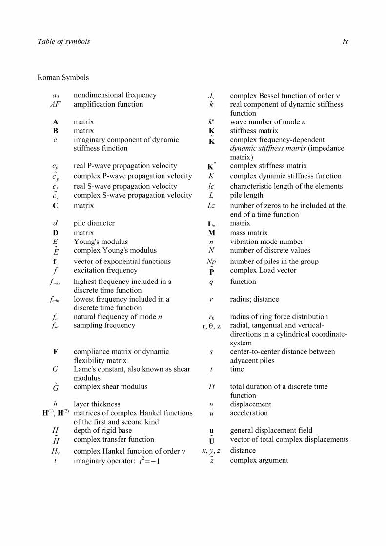
Table of symbols ix
Roman Symbols
a0 nondimensional frequency Jν complex Bessel function of order νAF amplification function k real component of dynamic stiffness
functionA matrix kn wave number of mode nB matrix K stiffness matrixc imaginary component of dynamic
stiffness functionK complex frequency-dependent
dynamic stiffness matrix (impedancematrix)
cp real P-wave propagation velocity K* complex stiffness matrixc p complex P-wave propagation velocity K complex dynamic stiffness functioncs real S-wave propagation velocity lc characteristic length of the elementscs complex S-wave propagation velocity L pile lengthC matrix Lz number of zeros to be included at the
end of a time functiond pile diameter Lσ matrixD matrix M mass matrixE Young's modulus n vibration mode numberE complex Young's modulus N number of discrete valuesf1 vector of exponential functions Np number of piles in the groupf excitation frequency P complex Load vector
fmax highest frequency included in adiscrete time function
q function
fmin lowest frequency included in adiscrete time function
r radius; distance
fn natural frequency of mode n r0 radius of ring force distributionfsa sampling frequency r, θ, z radial, tangential and vertical-
directions in a cylindrical coordinate-system
F compliance matrix or dynamicflexibility matrix
s center-to-center distance betweenadyacent piles
G Lame's constant, also known as shearmodulus
t time
G complex shear modulus Tt total duration of a discrete timefunction
h layer thickness u displacementH(1), H(2) matrices of complex Hankel functions
of the first and second kindu acceleration
H depth of rigid base u general displacement fieldH complex transfer function U vector of total complex displacements
Hν complex Hankel function of order ν x, y, z distancei imaginary operator: i2=1 z complex argument

x
Greek symbols
α pile inclination with the vertical Γ Gamma functionαn participation factor of mode n λ Lame's constantβ hysteretic damping coefficient λs wavelength of s-waveχ angle µ arbitrary term of the Fourier seriesδ displacement ν Poisson's ratio∆ matrix ρ mass density∆f frequency increment θ angle∆t time increment ω circular frequency of the excitation ε dilatation of a volume element ωn circular natural frequency of mode nφ discrete modal shape ω rotation of a volume elementγ function ψ function

1. Introduction 1
1. Introduction
1.1 Research motivation
Earthquakes are caused by an energy release in a particular location, hereafter referred as source,
inside of the Earth's crust. The energy travels in form of waves and propagates away from the
source into all directions. Different phenomena occur with the wave propagation. The energy
attenuates with the distance from the source when the wave travels inside of a homogeneous
medium. Besides, the presence of material discontinuities inside the medium allows the reflection
and refraction of the waves, which may change the direction, the amplitude and the type of the
wave. The waves induce oscillating movements of the medium. When the waves reach the vicinity
of the ground surface, these movements are transmitted through the soil to structures, which may
suffer damage or even collapse.
Because of the energy dissipation with the distance, the amplitude of the movements is expected to
reduce with the distance from the source. However, soft soils located at a relatively low depth from
the ground surface amplify the incoming movement, even if located relatively far from the source.
If the surface soil layers are composed from loose saturated sands, liquefaction may occur. The soil
then behaves like a fluid, unable to carry shear forces. Soft saturated clays subjected to high
amplitude cyclic deformations are not able to suffer liquefaction, but may experience partial loss of
shear strength; in some cases, they have displayed a relatively elastic behavior (Romo, 1995).
In case of static loads, soft soils present low load capacity and high deformability. This is usually
compensated using special foundation systems. The stress increment from the structure to the soft
soil layers should be reduced, distributed and/or transmitted through the foundation to deep stiffer
soil layers, in order to maintain the settlements at an acceptable level. For this purpose, pile
foundations are often selected. Although these foundations are selected to fulfill static load bearing
and deformation requirements, they often are also exposed to seismic loads.
The dynamic behavior of pile foundations has been a research topic in the last 30 years. Analytical,
numerical, experimental and field research has been developed. However, different case studies
published in the last years, report both acceptable and unacceptable seismic behavior of structures
supported on pile foundations. Different explanations have been associated to this dual behavior. It
seems clear that the seismic behavior of structures founded on pile foundations is still not fully
understood.

2
It has been traditionally assumed in seismic engineering that most of the energy of the earthquakes
is transmitted through waves which produce horizontal movements of the soil and of the nearby
structures. Most of the seismic codes in the world allow to neglect the effect of vertical seismic
excitation in structures, during the design process. However, it has recently been observed that in
the case of locations relatively near to the source, the magnitude of the peak ground vertical
accelerations can be higher than the horizontal ones. In such cases, typical failure mechanisms have
been detected that can clearly be attributed to a vertical excitation. Therefore, if high amplitude
vertical accelerations are expected in a location, they must not be neglected.
Techniques to reduce vibrations in structures subjected to dynamic excitations (also called
vibration control) have been developed. According to the requirements of exterior energy for its
performance, three groups can be made out: passive devices, which do not require exterior energy
and their behavior is defined only by their mechanical configuration; active devices, which require
exterior energy and often consist of force delivery devices integrated with evaluators, controllers
and sensors within the structure (Soong, 2000); and, hybride devices, which behave as an active
system for small deformation amplitudes and as a passive device for middle and high deformation
amplitudes. Seismic excitations are typically characterized by short duration and strong motion
amplitudes. In recent years, the use of active solutions for structures subjected to seismic
excitations has increased. However, essentially to their higher robustness, passive and hybride
devices are still preferred over active devices to protect structures subjected to seismic excitations.
In all cases, structural control procedures usually consist of a modification of the structural
behavior through the inclusion of an external device. Little efforts have been done in order to
design the structure in such a way that an internal subsystem adopts the behavior of a vibration
control device.
1.2 State of the art
The following state of the art is divided into the three main topics of this dissertation: seismic
excitations and its influence on the behavior and failure modes of typical structural systems;
numerical analysis of the seismic behavior of structures supported on pile foundations in soft soil
deposits; and, passive vibration control techniques usually employed to protect structures
potentially subjected to seismic excitations.

1. Introduction 3
1.2.1 Structural behavior under seismic excitation
So far it has been normal to neglect the vertical excitation for the seismic design of structures. This
has been supported by the observation that the vertical amplitudes of the seismic waves attenuate at
a higher proportion with the distance of the source than the horizontal waves do. Only few seismic
codes in the world suggest the consideration of the effect of vertical seismic excitation except for
cantilever members and long spans. Where vertical loads are considered, they are specified as
being equal to 0.5 or 0.67 of the horizontal earthquake loads (Elnashai et al., 1998).
For locations relatively close to the seismic source, the excitation is defined as a near-source
earthquake. The investigations from the recent near-source earthquakes have shown a different
behavior of the vertical component of motion. Elnashai et al., (1998) reported that the ratio of the
recorded vertical-to-horizontal accelerations from many strong motions frequently exceeds unity.
Chouw (1998) observed a considerable higher frequency content of the vertical acceleration
component in comparison with that from the horizontal acceleration component of near-source
earthquakes.
The current practice that the security factor for gravitational loads could guarantee an acceptable
structural behavior under seismic excitations has been contradicted in the recent years. Papazoglou
et al., (1996) compared failure patterns observed in buildings and bridges after near-source
earthquakes with analytical results. They established that structural failure may ensue due to the
effect of vertical motion on shear and flexural response. Ghobarah et al., (1998) made numerical
simulations until a collapse limit in low- and medium-rise reinforced concrete buildings. It was
shown for the studied cases that the vertical ground motion can cause reduction in ductility and
increase in the story drift and damage levels. Elnashai et al., (1998) concluded from numerical
simulations that the vertical motion may reduce the shear and flexural capacity of reinforced
concrete frames considerably. They also observed that the compressive force demand increased by
over 100% in compression, while tension was often detected in columns. The nonlinear three-
dimensional numerical simulation of the inelastic behavior of reinforce concrete bridge piers during
Great Hanshin earthquake, pointed out that the vertical motion caused a change from flexural to
diagonal shear failures (Abdelkareem et al., 2000).
Papaleontiou et al., (1993) analysed structures, flexible in the vertical direction, located close to the
seismic source and subjected to earthquakes with high frequency content. They concluded that
vertical accelerations can control the axial forces and bending moments in the columns of the upper
stories of tall frames as well as the axial forces in most columns of short frames.

4
1.2.2 Numerical simulation of seismic behavior of structures on pile foundations
For the simulation of the dynamic behavior of soil-pile systems different analytical and/or
numerical approaches have been proposed. Exact solutions can be reached only through purely
analytical formulations. However, analytical formulations for typical problems are usually
complicated, because of their geometrical and mechanical configuration. They require very high
efforts and often still unknown strategies to be solved. Therefore they are seldom employed. The
assumption of mechanical simplifications or the recursion to mathematical simplifications allow to
reach solutions. Their accuracy depends mainly on the differences between the physical model and
its mathematical and mechanical formulation. These strategies are known as numerical
formulations. They all account for the different nature between the piles and the soil, consider
different assumptions for each of them and express the total system behavior as a coupled
formulation of the individual subsystems.
Piles are always represented through discrete models constituted of beam elements. However, each
numerical method uses a different model to represent the soil. Two main groups can be identified:
the continuos-media models and the simplified models.
The continuos-media models are usually formulated in the frequency-domain and allow to consider
the radiation into infinity, but strictly only in a linear way. The direct simulation of nonlinear
behavior is possible only in time domain formulations. Simulation of nonlinear behavior in
frequency domain is possible through a hybrid time-domain formulation or in approximated way
through the equivalent linear method. The mathematical approximation assumed allows a new
subdivision into three groups: The Boundary Element Method, the Thin Layer Method and the
Finite Element Method. These three groups as well as the simplified models will be briefly
addressed.
1.2.2.1 Boundary Element Method
The Boundary Element Method states a mathematical formulation of the infinite soil based on
fundamental solutions. These are often obtained analytically and only for homogeneous media. The
method is suitable to solve problems involving only a homogeneous halfspace because no
discretization inside of the halfspace but on the surface is required to obtain the solution. Material
discontinuities can be handled through a coupling of regions. Material energy dissipation is handled
in the Fourier-domain through a hysteretic damping formulation (Kaynia 1982, Mamoon et
al., 1990), or in Laplace-domain through Kelvin chain models (Hillmer 1987, Chouw 1994).

1. Introduction 5
Formulations of this type have been developed for both single piles and pile groups in
homogeneous media for static loading (Poulos 1968 and 1971, Butterfield & Banerjee 1971), and
for dynamic harmonic loading (Kaynia 1982, Mamoon et al., 1990, Guin 1997).
Most of the formulations based on the Boundary Element Method to manage the dynamic soil-pile
interaction problem are able only to handle homogeneous halfspaces. Exceptions constitute those
based on the Green functions proposed by Kaynia (1982) developed for a layered medium over a
halfspace. Although these Green functions are formulated explicitly, they must be evaluated in a
numerical way. The restrictions in the formulation presented by Kaynia (1982) were: The contact
between the pile cap and the ground surface was not considered; and, no superstructure was
considered.
1.2.2.2 Thin Layer Method
The Thin Layer Method describes soil deposits through a semi-analytical formulation. A historical
review is reported by Kausel (1999). It was originally developed for layered soil deposits over rigid
bases. However, the simulation of a viscoelastic underlying halfspace is possible either through the
variable depth method along with the inclusion of a viscous boundary (Lysmer et al., 1988a) or in
terms of para-axial approximations (Seale & Kausel, 1989). The Thin Layer Method requires the
discretization in only one direction, i.e. in the stratification direction. It employs closed form
solutions in the horizontal plane. Transmitting boundaries were formulated in the frequency-
domain in a matrix form for plane (Waas 1972) and cylindrical coordinates (Kausel 1975). They
consider the infinite lateral extension of the media and can be coupled with the algebraic
formulation of a discrete central region. This formulation is exact in the horizontal direction but
depends on the discretization and the assumptions taken in the vertical direction. Solutions are
formulated in the frequency-domain for the displacements due to dynamic forces acting in or on a
layered media (Waas 1980, Tajimi 1980, Kausel 1981, Kausel & Peek 1982, Waas et al., 1985).
The most complete formulation of the Thin Layer Method to manage dynamic soil-pile interaction
problems is the one proposed by Hartmann (1986), Waas & Hartmann (1984), and Waas &
Hartmann (1981). They formulate the soil-pile behavior in terms of the uncoupled flexibility
matrixes of the soil and of the pile and impose further additional boundary conditions to reach the
coupling. Steady state harmonic behavior as well as seismic behavior of pile foundations was
simulated. The inertial seismic behavior of the superstructure in the horizontal direction was
simulated in a simplified way only with a concentrated mass (rigid body assumption) and without
consideration of the coupled rocking moment. The restrictions of this formulation are: they assume

6
an uncoupled translational and rotational behavior for the flexural deformation of the piles; because
of the coupling scheme, they are not able to simulate a flexible head plate; and, finally, they did not
consider the contact between the pile head plate and the ground surface.
1.2.2.3 Finite Element Method
The finite element formulation in dynamic soil and foundation problems, implies a step further in
the approximations for the definition of the soil media. It requires a discretization and a finite
element definition of a determinate soil volume. This discretization alone would trap the energy of
the system and distort its dynamic characteristics. To avoid this problem, the finite element
formulation is often coupled with a transmitting boundary formulation, like the one described
above. The resulting formulation is usually referred as Dynamic Finite Element Method (Gazetas &
Milonakis 1998). The transmitting boundary simulates the wave propagation into the exterior semi-
infinite media and expresses the far field in terms of a free field behavior (isolated from the
interaction with any other mechanical system). In the original formulation, the transmitting
boundary was coupled with a discrete volume which included the foundation as well as the
surrounding soil affected by the interaction with the structure. Therefore, it was set relatively far
away from the foundation (Waas 1972, Kausel 1974). Further improvements were reached with the
Flexible Volume Method (Lysmer 1988a, Tabatabaie 1982) which included the definition of the
whole layered media in the mathematical formulation, avoiding the requirement to set the
transmitting boundary relative far away from the foundation. The transmitting boundary was then
attached to a more simple discretization: a vertical column of quadrilateral elements for 2-D
configurations and a vertical column of cylindrical elements for 3-D configurations. The
mechanical formulation of this discrete region was expressed in terms of finite element
approximations. This formulation was repeated on every common soil-foundation node to compute
the stiffness matrix of the whole layered media.
The dynamic finite element formulation in combination with the Flexible Volume Method has been
applied to analyse the dynamic behavior of soil-pile systems (Ostadan 1983). Two formulations
were presented: One formulation, identified as the full method, introduces finite elements to model
the soil between the piles (inter-pile elements). Vertical and inclined piles as well as direct applied
forces or seismic excitations may be considered. The other formulation, identified as the simplified
method, does not require the inter-pile elements. The simplified method may simulate only vertical
piles under dynamic forces acting at the piles. It is evident that the full method is more versatile
than the simplified method. However, two are the main limitations of the full method: on the one

1. Introduction 7
hand, as it was stated above, the formulation of the soil media requires a discretization of a soil
volume and therefore increase the approximation level in one (for the plane deformation problems)
or two dimensions (for the spatial deformation problems) with respect to the semi-analytical
formulations (Thin Layer Method). On the other hand, the discretization required for the soil
volume between piles generally increases the number of the required nodes and therefore the
computational time and memory required.
1.2.2.4 Simplified models
The simplified models include a variety of approximations and semi-empirical approaches, also
referred as Winkler models or "beam on dynamic Winkler foundation". They adopt the static
Winkler simplification of soil structure interaction to the dynamic formulation: They assume the
dynamic soil action on the foundation as a group of independent parallel spring-damper arrays in
the horizontal as well as in the vertical directions along the interface. In case of pile foundations,
the mechanical parameters for the spring damper devices are frequently obtained from experimental
results (p-y curve for lateral and t-z for axial loading), or from analytical and/or numerical results
from very simplified models. The two main limitations from these models are: on the one hand, the
infinite nature of the soil media is often neglected or too much simplified; on the other hand, the
models are unable to describe pile groups directly. Efforts to improve the description of the soil
media are formulations in the frequency-domain. They allow the definition of frequency dependent
parameters for the spring-damper device, but complicate the simulation of nonlinear behavior
(Gazetas et al., 1992, 1993; Makris & Gazetas 1992; Kavvadas & Gazetas 1993). Pile groups are
approximately simulated through the concept of the equivalent pier (Lok 1999, Reese 1984, Brown
et al., 1988) which is restricted to low values of pile spacing, or through simplified interaction
factors (Nogami 1985, Makris & Gazetas 1992, Novak 1994, Mylonakis 1995, El-Naggar &
Novak 1996, Mylonakis & Gazetas 1998). Formulations in the time-domain allow a relative simple
simulation of nonlinear behavior of soil-pile interface (slipping and gapping), through the inclusion
of nonlinear springs (Lok 1999).
1.2.3 Passive vibration control techniques against seismic excitations
The vibration control techniques usually employed to protect structures subjected to seismic
excitations have two disadvantages that deserve our attention. On the one hand, in its original
conception, they neglect the influence of the soil in the behavior of the structural system. On the
other hand, they have been developed and applied to protect structures only from the horizontal

8
component of earthquakes. Therefore, following two aspects will be addressed: passive vibration
control techniques for structures subjected to horizontal seismic excitations; and, vibration
reduction in structures subjected to three-dimensional seismic excitations.
1.2.3.1 Horizontal seismic excitations
Passive vibration control consists of the reduction of the vibration amplitudes and the dynamic
demand in a structure through the inclusion of purely mechanical devices. The performance of
these devices require no extra energy than the one supplied by the excitation. Two main
philosophies can be identified: frequency uncoupling and energy dissipation. They will be briefly
described. Besides, some remarks about the reduction of horizontally seismic induced vibration in
structures founded on soft soils will be stated.
Frequency uncoupling
Probably the best known technique of frequency uncoupling is base isolation. It is a design strategy
that uncouples the fundamental vibration of the structure from that of the ground motion. (Naeim &
Kelly 1999) The uncoupling is normally achieved through the inclusion of soft springs (structural
elements with low horizontal stiffness) between the structure and the foundation. This reduces the
fundamental frequency of the structure. The reduction in the structural response will depend on the
uncoupling reached between the structural fundamental frequency and the high amplitude
frequency range of the ground motion. In an optimal performance, the fundamental mode of the
isolated structure should be characterized by deformations only in the isolation device, while the
structure behaves as a rigid body. No energy dissipation occurs, but rather an energy deflection due
to the dynamic frequency uncoupling. A selection of building applications in the United States is
reported by Buckle (2000).
Although the original concept was developed for seismic excitations, base isolation has been
applied to protect structures subjected to other type of excitations. Typical cases are excitation
forms which propagate through waves in the soil and incide in the structure in form of a support
excitation (man-made vibration in the vicinity of the structure). In such cases, base isolation can
protect a structure from the vibrations propagated through the soil. It can also be used at the source
to reduce the vibrations that will be propagated into the soil.
Energy dissipation
Energy dissipation techniques originated almost simulationeously as base isolation. Originally,

1. Introduction 9
their main objective was to restrict the displacements of the base isolation devices to an acceptable
level. At present, energy dissipation devices are used not only at the foundation level, but inside of
the structural system of building and bridges. Their function is to dissipate energy during a
dynamic excitation and to reduce the demand in the structure. However, the inclusion of the
dampers increases the stiffness of the main frame. If this contribution is big in comparison with the
stiffness of the frame, the effect may be detrimental. In contrast with base isolation, energy
dissipation devices can be applied not only for dynamic support excitations but also for excitations
that impinge direct on the upper part of the structure (for example wind).
According to their performance, energy dissipation devices can be classified as hysteretic or
viscoelastic. Hysteretic devices dissipate energy through the yielding of metals due to flexure,
torsion, or extrusion (metallic dampers) and sliding (friction dampers). They are essentially
displacement-dependent devices. Viscoelastic devices are composed either from special materials
(viscoelastic solids or viscoelastic fluids) or with a particular geometric configuration (fluid
orificing dampers). They are essentially velocity-dependent devices.
A common application of both concepts, frequency uncoupling and energy dissipation, is reached
through the tuned mass dampers (TMD). They can be understood as a simple mechanical vibrator
composed of a mass, a spring and a damper. They are installed inside of the structural frame
(normally where the highest amplitudes are expected). The presence of this additional structural
subsystem includes an additional eigen-frequency to the total system. The mass and stiffness
parameters of the vibrator are selected in a way that a natural frequency (usually the fundamental)
of the main structure is shifted. Therefore, two natural frequencies lay relatively close between
them. The vibration amplitudes of these both modal shapes are then reduced through an adequate
selecting of the damping of the vibrator as well as the choice of a relatively high mass. At present,
few applications for earthquake loading have been implemented (Soong & Dargush 1997).
Modified versions of the tuned mass dampers have been proposed: Tuned liquid dampers (TLD)
substitute the mass through a liquid. Multiple tuned mass dampers (MTMD) are combination of
simple tuned mass dampers, that cover a wider frequency range than a single tuned mass damper.
Observations in soft soil conditions
Three features related with vibration reduction in structures founded on soft soils will be discussed:
conventional base isolation; nonlinear soil behavior observed, and vibration reduction procedures
considering wave propagation.

10
Regarding base isolation, the effectiveness of the procedure is related to the increase of the natural
period of the structure in comparison with the natural period of the structure without base isolation.
Deep soft soil deposits, like those present in Mexico City, usually have long natural vibration
periods. In case of a conventional base isolation of a low building, the isolated natural period of the
structure may coincide with the natural period of the soil deposit. In this case, conventional base
isolation would be harmful to the structure (Chopra 2001).
The observation of the seismic behavior of structures in Mexico City during the
September 19, 1985 earthquake (Romo et al., 2000) and in Los Angeles-Santa Monica region
during the 1994 Northridge earthquake (Trifunac & Todorovska 1998), have revealed a relatively
satisfactory behavior of structures founded in soft soils with a stiff embedded foundation. It was
believed that the plastic deformations in the soil due to the interaction with the stiff foundation
acted as an energy dissipation mechanism that in many cases restricted building damage.
Constructions on flexible foundations were more susceptible to damage. This suggests beneficial
effects of the nonlinear soil behavior due to the interaction with stiff embedded foundations during
strong seismic motions (Romo et al., 2000).
The obstruction of the wave propagation in a continuos media is the base of different vibration
reduction procedures. They have been developed to protect structures subjected to excitations that
propagate through soft soils. They consist of the inclusion of an external device in the path the
wave propagates, between the source and the structure to protect. They are not connected directly
to the structure. The mechanic configuration of the device should be able to shield, to modify the
path or to attenuate the amplitude of the incident wave. Rigid devices such as a concrete block
(Chouw 1994), a concrete wall (Haupt 1978), and a barrier of piles (Aviles & Sánchez
Sesma 1988) have been proposed. Flexible devices, like open trenches (Dolling 1970) and gas
cushion mates (Massarsch 1991) have also been analysed. However, due to the usually high
amount of energy released during an earthquake, they have not been applied for earthquake
excitations.
1.2.3.2 Vertical seismic excitations
Only few applications of base isolation are reported in the literature as vibration control due to
vertical seismic excitation.
Fujita et al., (1996) proposed the use of coned-disc springs to protect structures from vertical
accelerations. Laboratory results indicated beneficial effects for secondary systems, but detrimental

1. Introduction 11
effects in the main structure. Yabana et al., (2000) proposed the use of special multilayer
elastomeric bearings. The vertical stiffness of the bearing was reduced through rubber layers of
higher thickness than those used only for horizontal seismic excitations. Laboratory results
indicated an acceptable performance for the particular case studied. Nawrotzki (2000, 2001)
proposes the use of helical steel springs together with viscodampers, to protect structures subjected
simultaneously to vertical and horizontal seismic excitations.
1.3 Objectives of the dissertation
1.3.1 Numerical model
A numerical model and a computer program should be developed to simulate and to predict the
dynamic linear damped behavior of structures supported on foundations with any geometric
configuration in layered subsoil conditions. Special attention should be given to a sufficient
representation of pile foundations.
Considering the general soil-structure system, the model should be able to simulate:
• linear behavior between load and response,
• material energy dissipation in the structure and in the soil, and
• coupled dynamic behavior between the semi-infinite soil media and the finite structure.
Considering the soil media, the model should be able to simulate:
• the dynamic frequency-dependent behavior of a semi-infinite soil media, and
• horizontally stratified media.
Regarding the structure, the model should be able to simulate:
• an arbitrary materials distribution,
• an arbitrary geometric configuration, and
• an arbitrary flexibility distribution.
Regarding the load, the model should be able to simulate:
• harmonic and nonharmonic excitations, and
• externally applied loads (forces and moments) or motions caused due to propagation of seismic
waves (earthquakes, traffic- and machine induced vibrations).
12
1.3.2 Simulation of the seismic behavior of soil-structure systems
With the help of the numerical model developed, the seismic behavior of structures supported on
deep foundations should be investigated. Special attention should be given to:
• horizontal and vertical seismic excitations,
• the observation and prediction of the resonance frequencies of the soil-structure system that
induce the natural vibration shapes in the structure, and
• the observation of the main components of the seismic behavior of soil-structure systems: the
kinematic and the inertial components corresponding to the foundation, as well as those
corresponding to the superstructure.
1.3.3 Seismic vibration reduction
Based on the observation of the seismic behavior of soil-structure systems, a vibration reduction
strategy should be proposed. Following conditions should be considered:
• the structure should be protected from both horizontal and vertical seismic excitations,
• the strategy should be applicable to structures founded on soft soil deposits,
• the strategy should be restricted to passive vibration control, and
• advantage should be taken from the structural arrangement of the system to be protected. No
extra device should be included.
To the best of the author's knowledge, the inclusion of the soil behavior in a seismic vibration
reduction technique has not been done to the present.
1.4 Structure of the dissertation
The seismic behavior of subsoil deposits, without considering the interaction with any structure
(free field) is the topic of chapter 2. The wave propagation in soils according to the theory of
elasticity is briefly reviewed. Considerations for the definition of the seismic environment as well
as the fundamentals of one-dimensional wave propagation in a soil layer over a halfspace are
stated.
Chapter 3 is dedicated to the numerical formulation of the soil-structure interaction. The
assumptions taken are listed. The substructure technique applied is described. The mechanical
formulation of the equation of motion is stated. The application of the Thin Layer Method to
formulate the dynamic stiffness of the soil media is summarized. The evaluation of the free field
1. Introduction 13
displacements at the interaction nodes is briefly explained. The solution procedure for harmonic
and for nonharmonic loads is stated. General remarks about the computational procedure for the
seismic soil-structure interaction are listed.
Chapter 4 describes the implementation of the computational procedure. The computational
algorithm is numerically implemented and coupled with an existent computer program.
Generalities about the computational model and about the discretization criteria are commented.
The computational model is verified by comparing own results with those reported in the literature.
The seismic response of a soil layer over a rigid base without any structure (free field) is computed
in chapter 5. The transfer functions due to a harmonic acceleration at the rigid base are calculated.
The criteria used to select an input earthquake motion is described. An artificial acceleration
history is generated. The seismic acceleration histories at the surface of the soil layer due to the
input earthquake motion at the base are computed.
Considering a structure constituted only of a foundation, the soil-foundation interaction is
discussed in chapter 6. The dynamic behavior of three foundation systems, namely rigid surface
foundations, pile foundations (single piles and pile groups) and soil improvement blocks (here
considered as a foundation type), is numerically simulated and compared. For a subsoil condition
consisting of a soil layer over a rigid base, the transfer functions at the top of the foundation due to
a harmonic acceleration at the rigid base are computed. For two different subsoil conditions, one of
them consisting of a soil layer over a rigid base, and the other of them consisting of a homogeneous
halfspace, the dynamic stiffnesses of the foundations are calculated due to harmonic forces and
moments acting at the foundation top. Conclusions related to the ability of each investigated
foundation to reduce the near field amplitudes for the fundamental resonance frequency of the soil
deposit in the excitation direction are stated.
Considering a structure constituted of a foundation and a superstructure, the soil-foundation-
superstructure interaction is investigated in chapter 7. The subsoil conditions consist of a soil layer
over a rigid base. Under the assumption of a rigid superstructure on a surface foundation, the
transfer functions at the superstructure top due to a harmonic acceleration at the rigid base are
computed. It is illustrated how the structural resonance frequencies inside of the soil-structure
system can be identified. The transfer function at the top of the superstructure of frame buildings
with different number of storeys on surface foundations due to a harmonic acceleration at the rigid
base are computed. The influence of the soil in the structural resonance frequencies inside of the
soil-structure system is illustrated. The transfer functions at the top of the superstructure of a same

14
frame building on different foundation types (surface foundation, vertical pile foundation, inclined
pile foundation and short vertical pile foundation) due to a harmonic acceleration at the rigid base
are computed. The influence of the foundation type in the vibration amplitudes at the superstructure
top was investigated.
The reduction of seismic induced vibrations in structures using deep foundation is the topic of
chapter 8. Two design strategies are proposed. One of them is aimed at the reduction of vertical
vibrations in structures induced by vertical seismic excitations. The other one is dedicated to the
reduction of horizontal vibrations in structures induced by horizontal seismic excitations. Each
procedure is illustrated with an example. Conclusions are stated regarding the possibility of
considering the foundation as a passive vibration control device for the case of seismic excitation.
The conclusions and recommendations for future research are summarized in chapter 9.

2. Propagation of seismic waves in soils 15
2. Propagation of seismic waves in soils
Earthquakes are caused by different types of energy releases inside the Earth's crust. The energy
travels from the source outwards in all directions in form of waves. Earthquake engineers try to
predict the motion at the soil profile expected in a specific site. For this purpose, fundamentals of
wave propagation in soils are required. Additionally, assumptions should be made regarding the
location and the mechanism of the source in order to define its energy distribution, also known as
seismic environment. The seismic environment assumed, usually expressed as a superposition of
waves along with the geometrical and mechanical configuration of the soil profile, allows the
prediction of the motion amplitudes in the soil as a function of the motion amplitudes from the
source. This relationship is often called wave amplification in soils.
The evaluation of site-specific ground motions involves a number of steps that includes (Romo et
al., 2000):
• The identification of potentially active sources in the region.
• The evaluation of the seismicity associated with individual sources.
• The estimation of travel-path influences on the seismic wave characteristics as they propagate
from the source to the particular rock site.
• The computation of the dynamic response of soil deposits.
• The assessment of their stability when subjected to the design-level seismic environment.
The first three steps are related with geological and geophysical processes. They are out of the
scope of this investigation. Therefore, they are considered through very simple assumptions. The
attention is focused in the last two steps.
In this chapter, the basic concepts of seismic wave propagation and of amplification of seismic
motions in soils are stated.
2.1 Wave propagation in soils
According to the theory of elasticity, the dynamic equilibrium of a small element inside of an
infinite, homogeneous, isotropic, elastic medium, formulated in displacements, leads to two
equations corresponding to the so-called body waves: One equation describes the propagation of a
wave of cubical dilatation (also called primary wave, P-wave, compression wave, irrotational

16
wave), which induces a particle movement in the direction of the wave propagation (figure 2.1).
This equation is found to be (Richart & Woods 1970):
ρ ∂2 ε∂ t 2 =λ2G ∇ 2 ε , (2-1)
where ρ is the mass density, λ and G are the Lame's constants (G is also known as shear modulus),
t is the time, and ε is the volume dilatation that propagates with a velocity cp defined as:
c p= λ2Gρ
= E 1νρ1ν12 ν
, (2-2)
where E is the Young's modulus, and ν is Poisson's ratio.
Compression
Propagationdirection
Compression
x
y
z
Figure 2.1 Typical deformation pattern of a P-wave (after Haupt 1986).
The second equation describes the propagation of a wave of pure rotation (also called secondary
wave, S-wave, shear wave, equivoluminal wave), with a particle movement perpendicular to the
direction of the wave propagation. This solution is found to be:
ρ∂2 ωx
∂ t 2 =G∇ 2 ωx , (2-3)
where ωx is the rotation with respect to the x-axis, which propagates with velocity cs, defined as:
cs=Gρ= E
2ρ1ν. (2-4)
Similar solutions can be written for the rotations ωy and ωz .
From (2-2) and (2-4) it can be shown:
c p
cs= λ2G
G= 21ν
12 ν, (2-5)

2. Propagation of seismic waves in soils 17
which shows that cp is equal or higher than cs√2 for 0 < ν < 0.5 .
A further subdivision can be made for the S-wave according to the direction of the particle
movement: On the one side, the SV-wave is defined because the particle motion axis together with
the propagation direction define a vertical plane. On the other side, the SH-wave induces a particle
motion in a horizontal direction, which is perpendicular to a vertical plane common to the
propagation axis. Both S-wave types are exhibited in figure 2.2.
Propagationdirection
y
Shear
ShearPropagationdirection
x
y
z
(a)
(b)
Figure 2.2 Typical deformation pattern of a S-wave: a) SV-wave; b) SH-wave(modified after Haupt 1986).
In an elastic halfspace, the stress free surface allows the generation of a third type of wave, called
Rayleigh wave. The Rayleigh wave is confined to a zone near the boundary of the halfspace
(surface wave) and propagates parallel to the surface with velocity cR. The trajectories of the
particle motion are ellipses in the vertical plane common to the direction of propagation. The
magnitude and direction of the elliptical motion is dependent of the depth. On the ground surface,
the particles describe retrograde ellipses, as it is illustrated in figure 2.3.

18
Direction of Wave Propagation
1
w
u
Particle Motion
x
y
z
Figure 2.3 Typical deformation pattern of a Rayleigh wave on the ground surface(after Richart & Woods 1970)
The Rayleigh wave can be understood as a superposition of a horizontally propagating P-wave and
a horizontally propagating SV-wave, confined to a relatively short depth below the halfspace
surface. The relationship between cp, cs and cR is plotted in figure 2.4 as a function of the Poisson's
ratio.
cc
c/
=s
Figure 2.4 Relationship between cR , cs and cp as function of Poisson's ratio (afterRichart & Woods 1970).
The presence of discontinuities inside the medium such as soil layer boundaries or material changes
induces changes in the propagating wave in form of reflection and refraction, which may modify
the direction and the type of the reflected/refracted wave with respect to those from the incident
wave, according to Snell's law, which is schematically represented in figure 2.5.
In case of a layered halfspace, multiple total reflections within the upper layer can allow a second
type of surface wave called Love wave. The Love wave travels parallel to the halfspace interface
and generates a particle motion perpendicular to the propagation direction in the horizontal plane.
The Love wave can be understood as a horizontally propagating SH-wave confined to a short depth

2. Propagation of seismic waves in soils 19
with respect to the surface. The Love wave travels with a velocity cL, which is higher than the
shear-wave velocity of the surface layer and lower than the shear-wave velocity of the next lower
layer. A Love wave will not occur if the shear wave velocity of the surface layer is higher than the
shear wave velocity of the next lower layer.
Figure 2.5 Reflection and refraction of a wave at a layer interface according toSnell's law (after Richart & Woods 1970).
2.2 The seismic environment
One of the main problems for earthquake engineers is the determination of the spatial and temporal
variation of seismic motions in a soil profile given the motion at a single point.
The motions measured at the ground surface generated by a source in the Earth's crust are known to
be a superposition of different types of waves. The specific way the seismic waves are
superimposed is assumed to be a function of different variables such as the geometrical
configuration and mechanical parameters of the subsoil considered, the location and depth of the
source with respect to the observation point, as well as the earthquake mechanism of the source. If
all these variables are known, two questions arise: The energy distribution from the source in the
different wave types generated, and, for every wave type, the decrease of the energy density or the
displacement amplitude with increasing distance from the source, also called geometrical
attenuation.
Some investigations have taken place within the theory of elasticity for loads acting on the surface
of a homogeneous, isotropic, elastic halfspace. Regarding the first of these points, Miller &
Pursey (1955) studied the case of a vertically oscillating, uniformly distributed, circular energy
source on the surface of a homogeneous, isotropic, elastic halfspace and determined the distribution
20
of total input energy among the three elastic waves to be: 67% Rayleigh wave, 26% shear wave,
and 7% compression wave. Similar investigations for vertically oscillating, infinitely long energy
sources (two-dimensional problem) acting on the surface of an elastic halfspaces exist (Le
Houedec 1980).
Concerning the geometrical attenuation, Ewing, et al., (1967) showed that for point sources, the
amplitude of the body waves decreases in proportion to the ratio 1/r, where r is the distance from
the input source. Exception constitutes the propagation of body waves along the surface of the
halfspace, where the amplitude decreases as 1/r2. The amplitude of the Rayleigh wave decreases as
1/√r. In case of line sources, Le Houedec (1980) reported a geometrical damping for the body
waves as function of 1/√r3, and no geometrical damping for Rayleigh waves.
Despite the simplifying assumptions in the theory of elasticity and the differences existing with
respect to real soils, these investigations suggest the importance of the consideration of Rayleigh
waves for dynamic loads acting on the surface of soil deposits.
However, seismologists still have not reached agreement on how the different wave types should be
superimposed in order to realistically predict earthquake motions at a specific location, mainly due
to the uncertainties related with the location and the behavior of a potential source.
Geotechnical and seismic engineers usually make the following assumptions (Kramer 1996, Chen
et al., 1981):
When a motion is produced by a source in the Earth's crust, body waves travel in all directions. As
they reach boundaries between different materials, they are reflected and refracted. Since the wave
propagation of shallower materials are generally lower than the materials beneath them, inclined
propagating waves that strike horizontal layer boundaries are usually reflected to a more vertical
direction (chapter 2.1). For locations relatively close to the source, an inclined incidence of both
compression and shear waves is expected near the ground surface, and a significant part of the
ground surface motion can be attributed to the surface waves. On the opposite, for locations
relatively far away from the source, the wave reaches the ground surface almost vertically,
reducing the possibility of generation of surface waves, as it is illustrated in figure 2.6.
Surface waves have been registered in some earthquakes (Trifunac 1971, Anderson 1974,
Hanks 1975). Analytical and numerical methods exist to compute the free field motion of any
combination of inclined body waves and/or surface waves (Chen et al., 1981, Roesset 1977, Wolf
et al., 1982a and 1982b, Shinozuka et al., 1983). Numerical methods able to solve the soil structure

2. Propagation of seismic waves in soils 21
interaction problem considering general seismic environments are also available (Gómez-Massó et
al., 1983, Chen et al., 1981, Lysmer et al., 1988a and 1988b, Beskos &Tassoulas 1984).
Figure 2.6 Idealized relationship between earthquake source, wave path and subsoilconditions (after Chen et al., 1981).
Numerical investigations (Gómez-Massó et al., 1983) have shown the relative importance of the
consideration of Rayleigh waves in the seismic environment, in particular for shallow-embedment
structures built in rock. However, they have also justified the neglect of the Rayleigh waves for
shallow-embedment structures built in relatively soft soils.
In practice, seismic environments are usually assumed to be composed exclusively of vertically
propagating body waves. Two observations justify this assumption (Gómez-Massó et al., 1983):
Rayleigh waves have not been observed in the frequency range above 1 or 2 Hz, and thus need not
to be considered, since the frequency range of interest of typical structures is 2-25 Hz. Besides,
calculations have shown that the seismic environments produced by slightly inclined body waves
and higher-mode surface waves are very similar to those produced by vertically propagating waves.
For the purposes of this investigation, a source located relative remote from the observation point
and a pure vertical wave propagation in the soil is assumed . No surface waves are considered.

22
2.3 One-dimensional seismic wave propagation
In case of an earthquake, the wave propagation from its source is essentially a three-dimensional
wave propagation problem. By assuming a line source, or by considering only the effects at some
distance from the source, the problem can be reduced to a two-dimensional one, where all the
waves propagate in directions parallel to a plane (for example the x-z plane), and the motion is
therefore independent of the third coordinate (y direction). These waves will be referred hereafter
as plane waves. It has been shown (see e.g. Roesset 1977), that in the case of plane waves, the
displacement in the direction normal to the propagating plane (y direction) is uncoupled from the
displacements in the two normal directions defining the propagating plane (x and z directions). The
first one describes the propagation of SH-waves, while the other two are functions of both SV- and
P-waves. In general, a coupling between SV- and P-waves exists, when they are reflected and/or
refracted at the free surface or at a layer boundary (chapter 2.1). However, a further simplification
is introduced if the direction of propagation is assumed to be vertical. The problem becomes then a
one-dimensional case and each one of the components of motion is uncoupled.
Consider a vertically propagating SV-wave traveling upwards with a velocity cs from a rock base
through a single horizontal soil layer of thickness h. A material energy dissipation is assumed for
the soil in terms of a linear hysteretic damping β. This type of damping assumes complex elastic
parameters E and G of the form E 12 i β and G 12 i β , as well as complex wave
propagation velocities c p and cs of the form c p12 i β and cs12 i β , where i2=-1. The
amplification function AF 1ω , defined as the ratio of the amplitude of motion at the free
surface of the soil ux1(0) to the amplitude at the interface between soil and rock ux1(h), can be
written as (Roesset 1977):
AF 1ω=ux10ux1h
= 2exp i ω cs /hexp i ω cs /h
, (2-6)
where ω is the excitation frequency.
The resonance frequencies of the soil layer ωn can be found as:
ωn=2 n1π
2cs
h, (2-7)
where n is the resonance mode of the system. It can be seen that these resonance frequencies
depend only on parameters of the soil layer.
2. Propagation of seismic waves in soils 23
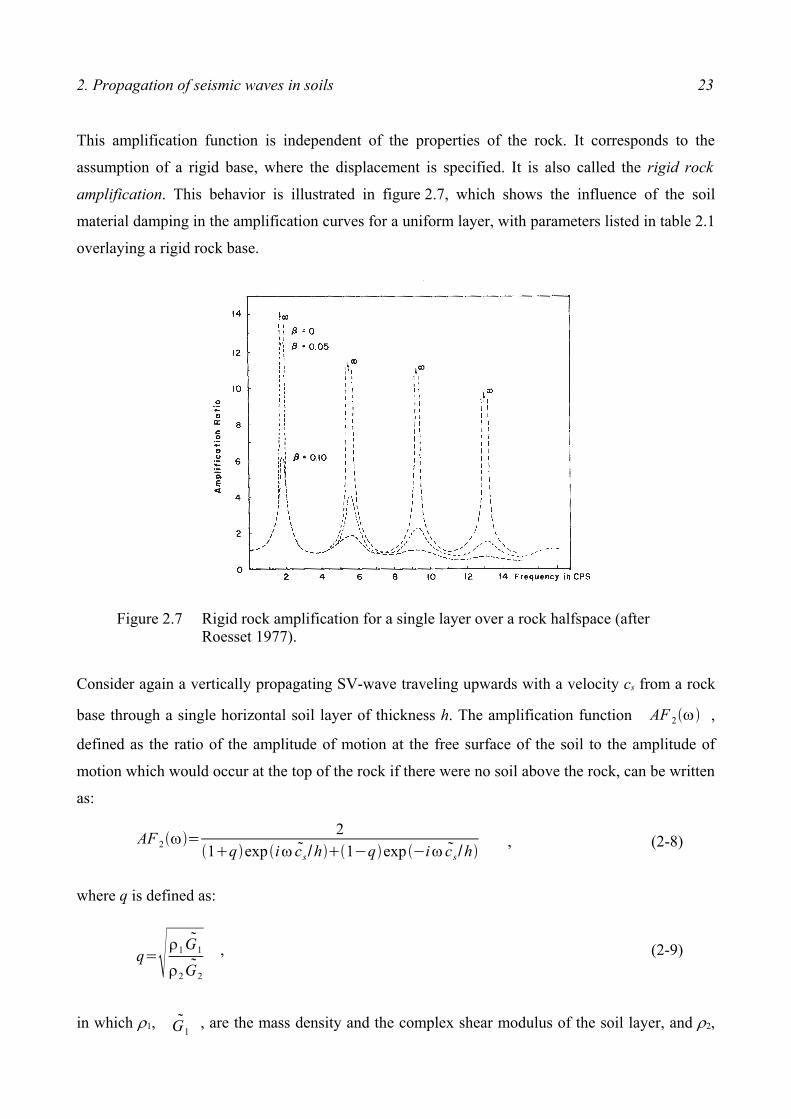
This amplification function is independent of the properties of the rock. It corresponds to the
assumption of a rigid base, where the displacement is specified. It is also called the rigid rock
amplification. This behavior is illustrated in figure 2.7, which shows the influence of the soil
material damping in the amplification curves for a uniform layer, with parameters listed in table 2.1
overlaying a rigid rock base.
Figure 2.7 Rigid rock amplification for a single layer over a rock halfspace (afterRoesset 1977).
Consider again a vertically propagating SV-wave traveling upwards with a velocity cs from a rock
base through a single horizontal soil layer of thickness h. The amplification function AF 2ω ,
defined as the ratio of the amplitude of motion at the free surface of the soil to the amplitude of
motion which would occur at the top of the rock if there were no soil above the rock, can be written
as:
AF 2ω=2
1qexp i ω cs /h1qexp i ω cs /h, (2-8)
where q is defined as:
q= ρ1G1
ρ2G2
, (2-9)
in which ρ1, G1, are the mass density and the complex shear modulus of the soil layer, and ρ2,
24
G2 are the mass density and the complex shear modulus of the halfspace.
Table 2.1 Subsoil mechanical parameters.
System cS ρ β H
[m/s] [kg/m3] [-] [m]Soil layer 228,6 2000,0 0.00, 0.05, 0.10 30,5
Halfspace (for AF2) 1371,5 2247,6 0,00 ∞
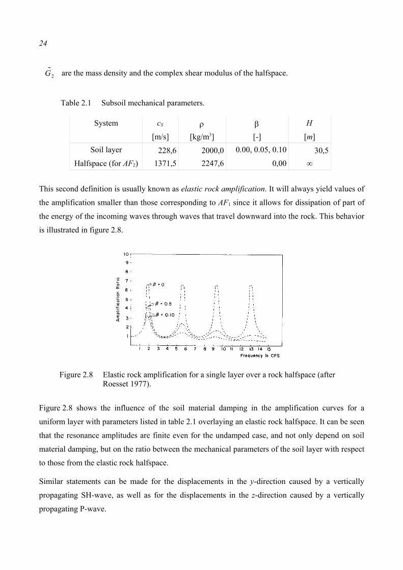
This second definition is usually known as elastic rock amplification. It will always yield values of
the amplification smaller than those corresponding to AF1 since it allows for dissipation of part of
the energy of the incoming waves through waves that travel downward into the rock. This behavior
is illustrated in figure 2.8.
Figure 2.8 Elastic rock amplification for a single layer over a rock halfspace (afterRoesset 1977).
Figure 2.8 shows the influence of the soil material damping in the amplification curves for a
uniform layer with parameters listed in table 2.1 overlaying an elastic rock halfspace. It can be seen
that the resonance amplitudes are finite even for the undamped case, and not only depend on soil
material damping, but on the ratio between the mechanical parameters of the soil layer with respect
to those from the elastic rock halfspace.
Similar statements can be made for the displacements in the y-direction caused by a vertically
propagating SH-wave, as well as for the displacements in the z-direction caused by a vertically
propagating P-wave.

3. Numerical formulation 25
3. Numerical formulation
The analyses of structures founded on or in soil deposits and subjected to dynamic loads is
addressed. The excitation can be defined as applied dynamic forces or as seismic excitations. The
loads are supposed to be known values. The deformations of the system are unknown.
Simplifications and assumptions are made in order to be able to solve the system with help of
numerical solution strategies. The following assumptions are made:
• The response is supposed to behave linearly with the load. This restricts the approach to small
displacement amplitudes and to linear material behavior. The principle of superposition and
Fourier transformation can therefore be applied.
• Damped elastic response is assumed for the soil as well as for the structure1.
• Material energy dissipation is introduced in form of a linear hysteretic damping formulation2.
• The soil media is supposed to be constituted of horizontal infinite layers.
3.1 Substructuring method
In the general case of embedded structures, three sub-regions are created for the purpose of
numerical modelling: the original soil deposit without the presence of the structure; the structure;
and the soil displaced for the basement, in the following called excavated soil (see figure 3.1). The
structure is again subdivided into a foundation (located at or below the ground level) and into a
superstructure (located above the ground level). The first sub-system, the soil deposit, is handled
with a semi-discrete technique called the Thin Layer Method (Kausel 1999). The second and third
sub-systems, the structure and the excavated soil, are described with the Finite Element Method
(Bathe 1974). The three subsystems are connected through the interaction nodes (nodes belonging
to all three subsystems). The assembly of the system is based on the Flexible Volume Method
(Lysmer et al., 1988a).
1 Different formulations could be used to simulate nonlinear behavior. General material nonlinear behavior could beapproximately considered through the linear equivalent method (Seed & Idriss 1969). Localized nonlinear behaviorand contact problems (often at the soil-structure interface or between two different structures) could be consideredthrough a hybrid time-frequency procedure (Wolf 1988, Dabre 1986, Hillmer 1987, Chouw 1994, Bode 2001).
2 This damping formulation is not dependent of the excitation frequency, but of the deformation amplitude.Considering a linear formulation, it may be inconsistent for the static case and for short duration transient loads(Hillmer 1987, Waller 1989, Chouw 1994, Peil 1993; Waas 1989). For periodic and relatively long durationtransient excitations (wind, earthquakes), it may be approximately used (Peil 1993).

26
(a) (b) (c) (d)
b b
i ii
s
Figure 3.1 Substructures of the system: a) total system; b) soil deposit; c) structure;d) excavated soil (modified after Lysmer et al., 1988a).
3.2 Equations of motion
The computational model is calculated in the frequency domain, where the input (loads) and output
(displacements) are connected to the time domain through the Fourier transformation. We consider
a simple harmonic component with an excitation circular frequency ω.
The equation of motion of the system is given by:
K U= P , (3-1)
where indicates complex values, U is the vector of total displacements at the nodal points, P
is the loads vector, and K is the complex frequency-dependent dynamic stiffness matrix or
impedance matrix (in the following called dynamic stiffness matrix) defined by:
K=K*ω2 M , (3-2)
in there M is the mass matrix and K* is the complex stiffness matrix defined by:
K*=K 12 i β , (3-3)
where K is the stiffness matrix, β is the damping ratio of a linear damping hysteretic formulation,
and i2=1 .
Two excitation conditions are possible: prescribed loads (hereafter referred as load excitation), and
3. Numerical formulation 27
prescribed motions (later called support excitation). Typical example of a support excitation are the
motions of a building foundation induced by earthquakes, which constitute the main excitation type
considered in this investigation.
In case of a load excitation, forces and/or moments can be acting at any point of the system. A
detailed formulation of the equation (3-1) is (Lysmer et al., 1988a):
[ K sss K si
s
K iss K ii
s K iid K ii
e ]{ Uss
Uis}={Ps
s
Pis} . (3-4)
The subscripts s and i correspond to the superstructure and to the interaction nodes. The
superscripts d, s and e correspond to soil deposit, structure and excavated soil, respectively. K iid is
the soil deposit dynamic stiffness matrix for the interaction nodes. K iis and K ii
e represent the
structure and the excavated soil dynamic stiffness matrices for the interaction nodes, respectively.
In case of support excitation, displacements and/or accelerations are prescribed at any point of the
system depending of the method of analysis. An earthquake consisting of body waves, can be
represented as the prescribed motion Ubd at the lower boundary b of the soil deposit (see
figure 3.1). The equation of motion of the substructure soil deposit is given by:
[ K iid K ib
d
Kbid Kbb
d ]{ Uid
Ubd}={Pi
d
Pbd} , (3-5)
where the sub-indice b corresponds to the lower boundary, Pid is the interaction load vector
between soil deposit and foundation and Pbd is the interaction load vector between soil deposit and
the lower boundary.
The equation of motion of the combined substructures structure and excavated soil is obtained
enforcing displacement compatibility Uis= Ui
e , and equilibrium Pis Pi
e=0 :
[ K sss K si
s
K iss K ii
s K iie ]{ Us
s
Uis}={ 0
Pis} . (3-6)
The equation of motion for the free field motion in the substructure soil deposit is:

28
[ K iid K ib
d
Kbid Kbb
d ]{ U 'id
U 'bd}={ 0
Pbd} , (3-7)
where the symbol ' indicates the free field condition, U ' id are the seismic free field
displacements at the interaction nodes. Substracting equation (3-7) from equation (3-5):
[ K iid K ib
d
Kbid Kbb
d ]{ Uid U 'i
d
Ubd U 'b
d}={Pid
0 } , (3-8)
and assuming a rigid lower boundary:
[ K iid ]{ Ui
d U 'id }={ Pi
d} . (3-9)
Introducing equation (3-9) in equation (3-6), the equation of motion for support excitation at the
lower base is given by:
[ K sss K si
s
K iss K ii
s K iid K ii
e ]{ Uss
Uis}={ 0
[ K iid ]{ U 'i
d }} . (3-10)
A linear damping hysteretic formulation is used for all three sub-structures. The dynamic stiffness
matrices for the structure and excavated soil are composed using the Finite Element Method
(Bathe 1974). The dynamic stiffness matrix for the soil deposit as well as the free field
displacements at the interaction nodes are computed using the Thin Layer Method. The latter will
be briefly introduced in the following.
3.3 The Thin Layer Method
The soil deposit is handled with a semi-discrete technique called the Thin Layer Method
(Waas 1972, Kausel 1974, Lysmer et al., 1988a). A historical review is reported by Kausel (1999).
The soil deposit is represented through infinite horizontal layers. It was originally developed for
layered soils over rigid bases (see figure 3.2). According to Kausel (1999), the Thin Layer Method
consists of a partial discretization of the wave equation, namely one in the direction of layering.
Hence, a finite element solution is used for that coordinate direction, while closed-form solutions
(or other numerical approaches) are used for the remaining coordinate directions.

3. Numerical formulation 29
8 8
free surface
layered medium
x
z
rigid base
Figure 3.2 Layered medium over rigid base.
A layered medium over a rigid base is discretized in N relatively thin layers with respect to wave
length. The free motion for a simple harmonic consists of a finite number of wave modes which are
obtained by the solution of an eigenvalue problem (Waas 1972). These wave modes serve as shape
functions for expanding the displacements in the media in terms of mode participation factors. The
forced motion due to applied loads or due to a prescribed displacement field is also expressed in
terms of such wave modes, where the participation factors are obtained after observing the
corresponding boundary conditions in terms of displacements and forces for the problem
considered.
In case of a plane deformation problem, the motions in the two orthogonal directions in the plane
are coupled and consist of generalized Rayleigh waves which may have real, imaginary or complex
wave numbers. The motions perpendicular to the plane consist of a generalized Love waves, and
may have real, imaginary or complex wave numbers. Rayleigh and Love waves in layered media
are described mathematically in the same way as generalized Rayleigh and Love waves,
respectively (see figure 3.3), but have real wave numbers.
Three-dimensional motion is expressed in terms of axisymmetric generalized Rayleigh and Love
waves and afterwards transformed to cartesian coordinates.
3.3.1 Eigenvalue problem
3.3.1.1 Generalized Rayleigh waves
A generalized Rayleigh wave for a plane deformation problem is defined by:
δ x=φ R x exp i ω tk R x , (3-11a)
δ z=φ R z exp i ω tk R x , (3-11b)

30
where δx and δz are the displacements in the x- and z-directions, φ R x and φ R z are the
corresponding discrete vertical deformation shapes assumed to vary linearly within each layer, ω is
the circular frequency of the simple harmonic, kR is its wave number and i2=-1. The exponential
function represents analytically the dependence on t and x.
P1
P2 1
2
j
j+1
N
1
2
j
j+1
N
P3
P4P2j-1
P2j
P2j+1
P2j+2P2N-1
P2N
P1
P2
Pj
Pj+1
PN
(a)
(b)
Figure 3.3 Degrees of freedom and corresponding nodal forces: a) generalizedRayleigh wave; b) generalized Love wave (after Lysmer et al., 1988a).
Formulating the strains, stresses, and inertial forces in terms of the layer interfaces displacements,
observing the boundary conditions at the free surface σ =0 and at the rigid base u=0 and
applying the principle of virtual work, the condition for equilibrium is obtained for the 2N degrees
of freedom in matrix notation as:
AR k R2i BR k RCR φ R=0 , (3-12)
which constitutes the one-dimensional (in z-direction) eigenvalue problem for the generalized
Rayleigh wave in the layered region, where kR are the algebraic eigenvalues already defined as
wavenumbers, and the vector φ R are the algebraic eigenvector representing the mode shapes,
which can be partitioned in the x- and z-degrees of freedom, to obtain φ R x and φ R z , respectively.
The matrices AR, BR and CR, as well as a solution technique to solve the eigenvalue problem, and
characteristics of both wavenumbers and vibration shapes are reported by Waas (1972). The

3. Numerical formulation 31
discrete layered media has 2N propagating generalized Rayleigh waves.
3.3.1.2 Generalized Love waves
A generalized Love wave for a plane deformation problem is defined by
δ y=φ L y exp i ω tk L x , (3-13)
where δy are the displacements in the y-direction and φ L y is the corresponding discrete vertical
deformation shape assumed to vary linearly within each layer, while the exponential function
describes analytically the dependence on t and x.
As for the generalized Rayleigh wave, formulating the strains, stresses, and inertial forces in terms
of the layer interfaces displacements, observing the boundary conditions at the free surface
σ =0 and at the rigid base u=0 and applying the principle of virtual work, the
equilibrium equation is obtained for the N degrees of freedom in matrix notation as:
AL k L2CLφ L y=0 , (3-14)
which constitutes the one-dimensional (in z-direction) eigenvalue problem for the generalized Love
wave in the layered region, kL is the algebraic eigenvalue already defined as wavenumber, and the
vector φ L y is the algebraic eigenvector representing the mode shapes. The matrices AL and CL, as
well as a solution technique to solve the eigenvalue problem, and characteristics of both
wavenumbers and vibration shapes are reported by Waas (1972). The discrete layered media has N
propagating generalized Love waves.
3.3.2 Free field displacements
The seismic response of the soil deposit is known as the free field solution. The computation of the
free field displacements at the interaction nodes proceeds through the formulation proposed by
Chen et al., (1981) which is based in the wave propagation formulation proposed by Waas (1972).
The soil model constitutes a layered media over a rigid base3. The seismic environment
(chapter 2.2) may be defined as a combination of body waves with any incident angle and/or
surface waves. In this investigation, a plane deformation state and a pure vertical wave propagation
in the soil are assumed. The deformation state induced by the assumed seismic environment in x-
3 Chen et al., (1981) simulates an underlaying damped elastic halfspace. The flexible boundary condition at thedeepest boundary is substituted by an interface force between the layered system and the halfspace. The equationsystem obtained is solved through static condensation procedures.

32
and z-direction is expressed as a modal superposition of the uncoupled deformations corresponding
to the generalized Rayleigh waves in the layered media, and in y-direction is expressed as a modal
superposition of the generalized Love waves in the layered media.
The free field displacements δ at the interaction nodes are expressed as:
• for a vertically incident SV-wave:
δ x=∑l=1
2 N
α Rl φ R x
l exp i ω tk Rl x , (3-15)
• for a vertically incident P-wave:
δ z=∑l=1
2 N
i α Rl φ R z
l exp i ω tk Rl x , and (3-16)
• for a vertically incident SH-wave:
δ y=∑l=1
N
α Ll φ L y
l exp i ω tk Ll x , (3-17)
where x is the distance from the interaction point to the control point (where the prescribed motion
is assigned), and αl is a mode participation factor for the mode l that can be found for the given
seismic environment at the coordinate x=0 for the frequency of analysis.
3.3.3 Green's functions of a layered medium
Waas et al., Kausel et al., and Tajimi (Waas 1980, Tajimi 1980, Kausel & Peek 1982, Waas et
al., 1985) have reported closed-form solutions of the three-dimensional Green's functions in a
layered medium over a rigid base. The load can be applied at any depth of the medium and may
have ring, disk or point force distributions with resultant force one.
Considering a general ring force distribution of the form p ω =p cos nθ⋅exp i ω t or
p ω =psin nθ⋅exp i ω t , acting in the radial, tangential or vertical direction as shown in
figure 3.4, the general displacement field u is expanded in a Fourier series:
u=∑µ=0
∞ { uρµsy cos µθ
uθµsy cos µθ
uz µsy sin µθ }{
uρµa sin µθ
uθµa sin µθ
uz µa cos µθ }exp i ω t ,
(3-18)

3. Numerical formulation 33
where uρµ, uθµ and uzµ are functions of r and z and represent the radial, vertical and tangential
displacements, respectively, the superscripts sy and a refer to symmetry and antisymmetry
about θ =0 , respectively, and µ is an arbitrary term of the Fourier series.
Formulating the strains, stresses, and inertial forces in terms of the layer interfaces displacements,
observing the boundary conditions at the free surface σ =0 and at the rigid base u=0 and
applying the principle of virtual work, Waas, et al., (1985) formulated the homogeneous equation
of motion of the layered medium:
Lσ D ∆ρ ω 2 Iu=0 , (3-19)
where ρ is the material density and I is a 3x3 identity matrix. The matrices Lσ, D and ∆ are
described by Waas et al., (1985). The solution is expressed in the form:
u=α1H1α2H2f 1 , (3-20)
where H1 and H2 are matrices of complex Hankel functions of the first and second kind,
respectively, f 1 is a vector of exponential functions dependent on k and z, while, α(1) and α(2) are
participation factors.
It is assumed a solution of the form:
u=α1H1α2H2f , (3-21)
where f is a vector of unknown functions dependent on z linearly varying in each sub-layer.
Introducing such assumed solution in the equation of motion, the algebraic one-dimensional
eigenvalue problems for generalized Rayleigh waves and for generalized Love waves, respectively,
discussed in section 3.3.1 are obtained, where f is found to be the mode shapes φRx, φRz and φLy.
The displacements ub along the interface r=r0 , are expanded in terms of the solutions of the
homogeneous problem:
ub=∑l=1
2 N
α Rl 1HR
l 1α Rl 2HR
l 2φ Rl ∑
l=1
N
α Ll 1HL
l 1α Ll 2HL
l 2φ L yl . (3-22)

34
r0
1
n
m
N
z
Pz
Pr
uzuru�
r
uz
ur
r0
Pr�
rP�
p = cos
p = sin
��
��
��p = cos
r
�
z
I II
Figure 3.4 Ring forces and displacements in layered medium over a rigid base(modified after Waas 1980).
Considering two regions: region I defined by rr0 , and region II defined by rr0 , observing the
wave propagation in every region and satisfying the displacement continuity and force equilibrium
along the interface r=r0 , the participation factors are evaluated and the displacements along the
boundary of the layer m, for ring loads at r=r0 on layer n, and for any Fourier term µ are given
by:
urmn={∑l=1
2 N
α Rnl φ x
ml dd r
f lRµ
r ∑l=1
N
α Lnl φ y
ml f lL}cos µθ
sin µθ , (3-23a)
uθmn={µ
r ∑l=1
2 N
α Rnl φ x
ml f lR∑
l=1
N
α Lnl φ y
ml dd r
f lL}sin µθ
cos µθ , (3-23b)
uzmn={∑l=1
2 N
α Rnl φ z
ml f lR k l}cos µθ
sin µθ , (3-23c)
where the undefined terms are listed in the appendix 2, as well as the expressions for different load
conditions (ring, disk and point load distributions), for different excitation directions and for
different displacement regions according to the formulation from Kausel & Peek (1982).

3. Numerical formulation 35
3.3.4 The soil deposit impedance matrix
The soil deposit impedance matrix K iid , in equations (3-4) and (3-10) is calculated as:
[ K iid ]=[ Fii
d ]1 , (3-24)
where Fiid is the soil deposit compliance matrix, also called soil deposit dynamic flexibility matrix.
Due to the frequency dependancy, the inversion is done for each considered frequency. The
elements fij of the soil deposit compliance matrix Fiid , are determined by successively applying unit
amplitude loads at each degree of freedom j of the interaction nodes and computing the
corresponding complex displacements (also known as compliances) at each degree of freedom i of
the interaction nodes, according to equation (3-23). They constitute the Green's functions of the
layered media for the interaction nodes (chapter 3.3.3).
The Green's functions on a layered medium for point loads allow directly the computation of a fully
three-dimensional site dynamic flexibility matrix useful for problems related with non-
axisymmetric massive foundations (Waas, et al., 1985). However, the solution for point loads is
singular on the vertical line passing through the loaded node. Therefore, a distributed load is used.
In order to simulate the load transfer from the foundation to the subsoil, a disk load distribution of
radius r0 is assumed for the nodes located on the horizontal and/or inclined soil-foundation
interfaces, while a ring load distribution of radius r0 is considered for the rest of the interaction
nodes. The distribution of disk and ring loads of radius r0 and the horizontal distance h between
neighbor interaction nodes are shown in figure 3.5.
x
zring load
disk load
A A,
B B,
Section A - A,
h
hr0
Section B - B,
x
y
Figure 3.5 Load distribution according to the location of the nodes for massivefoundations.
In case of pile foundations, the interaction nodes are selected along the pile axis.

36
A vertical pile display circular cross sections of radius r on horizontal planes. In order to simulate
the load transfer from pile to soil, a disk load distribution of unit amplitude and radius r0=r is
considered at the interaction node located at the pile tip, while ring load distributions of unit
amplitude and radius r0 are considered at the remaining interaction nodes.
A pile with radius r in its cross section and inclined an angle α with respect to a vertical line
displays ellipse cross sections on horizontal planes as it is shown in figure 3.6. The displacement
field of ellipse-shaped distributed loads is approximated in terms of the displacement field of
equivalent circular distributed loads. A disk load distribution with the same cross area as the
horizontal ellipse is considered at the interaction node at the pile tip.
++2r / cos ( )�
2r
2r
2r/cos( )�
�
x
z
x
y
(a) (b)Figure 3.6 Inclined pile: a) physical model; b) ellipse-shaped load distributions at the
interaction nodes.
The displacement field of distributed ellipse-shaped area loads uea in terms of the displacement field
of equivalent circular disk load distributions ucd of radius r0 is computed as:
uea= 1cosα ucd , (3-25)
A circle ring load distribution with the same circumference as the horizontal ellipse is considered at
the remaining interaction nodes. The displacement field of a distributed ellipse-shaped
circumference load uec in terms of the displacement field of equivalent circular ring load
distributions ucr of radius r0 is given by:
uec=1cosα2cosα ucr , (3-26)

3. Numerical formulation 37
The general displacement field computed in terms of the radial, vertical and tangential
displacements is transformed to cartesian coordinates through a transformation matrix.
3.3.5 Simulation of a homogeneous damped elastic halfspace
The formulation of the Thin Layer Method already described assumes a layered medium over a
rigid base. However, such formulation (with exception of the computation of the free field
displacements at the interaction nodes due to propagation of body waves) is applied to simulate a
layered medium over a homogeneous damped elastic halfspace through the variable depth method
together with a viscous boundary at the base (Lysmer et al., 1988a)4.
The variable depth method is based on the observation that the amplitude of the Rayleigh wave in
an homogeneous halfspace almost vanishes at a depth equal to 1.5 λR, where λR is the frequency-
dependent wavelength of the Rayleigh wave.
The method consists of the inclusion of n additional discrete layers below the top discrete soil
layers, hereafter referred as top layers. The additional discrete layers (referred as the bottom layers)
represent the halfspace and have a total thickness of 1.5 λs, where λs is the frequency-dependent
wavelength of the S-wave. Their thickness is frequency dependent. It is required the explicit
definition of at least one discrete layer with halfspace parameters with a frequency independent
thickness, belonging to the top layers. The selection of the frequency dependent thickness of the
bottom layers is described by Lysmer et al., (1988a).
The layer thicknesses of the bottom layers will increase with depth and decrease with frequency.
The layer thicknesses remain small as compared to the wavelength. The choice of n=10 has been
found to be adequate for all practical problems (Lysmer et al., 1988a).
The halfspace simulation is improved by replacing the rigid boundary on the bottom with a
frequency dependent viscous boundary. This consists of two dashpots per unit area of the
boundary. The selection of the damping coefficients is described by Lysmer et al., (1988a).
The physical and discrete model of a layered medium over a viscoelastic halfspace is exhibited in
figure 3.7.
4 An underlying halfspace can also be simulated in terms of para-axial approximations (Seale & Kausel 1989).

38
free surface
8 8
x
z
halfspace
.. . . . . .
rigid base
top layers:fixed thickness
bottom layers:frequency dependentthickness
dashpots
layered medium thin layers
(b)(a)
Figure 3.7 Layered medium over a viscoelastic halfspace: a) physical model; b) discretemodel (modified after Lysmer et al., 1988a).
3.4 Solution of the equation of motion
According to the nature of the load (harmonic and nonharmonic), two cases can be identified: a
steady state response analysis and a transient response analysis. The former will be discussed for a
harmonic load excitation, while the latter will be described for a nonharmonic support excitation
representing an earthquake excitation.
3.4.1 Response analysis due to a harmonic load excitation
The load is defined at discrete harmonic frequencies. The equation of motion is formed and solved
for each frequency component.
3.4.2 Response analysis due to earthquake excitation
An earthquake is simulated by prescribing at the base rock b (see figure 3.1), those vibration
amplitudes specifying the earthquake (see section 2.2). The analysis has two stages: a steady state
response analysis and a transient response analysis.

3. Numerical formulation 39
3.4.2.1 Steady state response analysis
For each frequency component, the response at each node j is computed in form of transfer
functions H j ω (also called unit complex frequency response functions) due to a unit base rock
vibration amplitude ∣ubω∣=1 :
H j ω =u j ω ubω
, (3-27)
where u j ω , are the vibration amplitudes at node j.
The free field displacements at the interaction nodes U ' id ω are computed as described in
section 3.3.2. They are further employed to compute equivalent seismic loads at the interaction
nodes, which constitute the excitation of the soil-structure system as formulated in equation (3-10).
The solution of equation (3-10) are the transfer functions H j ω .
3.4.2.2 Transient response analysis
The acceleration time history übt specifying the input earthquake and prescribed at the rigid
boundary is transformed to the frequency domain through the fast Fourier transformation FFT
(Cooley & Tukey 1965):
übt FFT° übω =ω 2 ubω , (3-28)
where übω and ubω are the acceleration and displacement complex Fourier amplitude spectra
at the rigid base, respectively. The complex Fourier amplitude spectrum ü j ω at each node j is
calculated as:
ü j ω =H j ω übω , (3-29)
which are transformed to the time domain through the inverse Fourier transformation IFFT (Cooley
& Tukey 1965):
ü j ω IFFT° ü j t
, (3-28)
in there ü j t is the acceleration time history at each node j.

40
To obtain a transient solution, ü j t , the transfer functions must be computed for all of the FFT
frequencies. To reduce the computational effort, the solution is obtained only for few selected
frequencies. The solution for the remaining frequencies is obtained using an interpolation technique
in the frequency domain, based in the vibration behavior of a two-degree-of-freedom system. The
procedure is given and described in detail by Tajirian (1981).
3.5 Considerations for the seismic soil-structure interaction
In this investigation, structures founded in a soft soil deposit overlaying a rock base are analysed.
The model configuration is displayed in figure 3.8, where the numbered points indicate the
representative locations where the response is observed. The rock is assumed to be rigid. The
analysis of the seismic soil-structure interaction includes the following three aspects:
• amplification of the seismic motion in the free field,
• soil-foundation interaction, and
• inertial interaction.
All three aspects could be analysed in a single step. However, in order to understand the complete
interaction, the three single aspects stated above will be analysed first separately.
The presence of soil layers overlaying rock deposits produce an amplification of the seismic
motions in the soil in comparison with that transmitted by the rock. The magnitude of this
amplification is a function of the mechanical and geometrical parameters of the soil and of the rock
(chapter 2.3). Although this phenomena is independent of the presence of the structure, it must be
considered in the soil-structure interaction to have the connecting loading.
5
2
rock base
body waves
4
6
8 8
1
2
free field
soil layer
foundation
superstructure
x
z
Figure 3.8 Configuration for seismic soil-structure interaction problems

3. Numerical formulation 41
The interaction between the structure stiffness and the soil is known as soil-foundation interaction.
To analyse it separately, only the foundation is considered instead of the whole structure. The
foundation stiffness restricts the deformation capability of the soil surrounding it.
The interaction between the dynamic stiffness of the structure and the soil is known as inertial
interaction. The acceleration field induces inertial forces in the structure, which are transmitted to
the foundation. They modify additionally the dynamic behavior of the system.

42
4. Implementation of the computational procedure
The system of computer programs SASSI: A System for the Analysis of the Soil-Structure
Interaction (Lysmer et al., 1988a and 1988b) is implemented with new computational modules
including the explicit formulations to compute the complex displacements for unit dynamic loads
(compliances) in the interior of a layered medium proposed by Kausel & Peek (1982)5. The system
of computer programs implemented in this dissertation is called SASSIG: A System for the
Analysis of the Soil-Structure Interaction using Green's functions. The evaluation of the soil
deposit compliances for three-dimensional problems using SASSIG requires only a one-
dimensional discretization of the soil deposit model (see sections 3.3 and 3.3.3), while the program
SASSI requires a two-dimensional discretization of the site model for the evaluation of the site
compliances for three-dimensional problems. The improvements give higher accuracy in the
analysis of the soil deposit impedance and allow directly the analysis of soil-pile interaction as it
was discussed in section 3.3.4.
In this chapter, the computational procedure described in chapter 3 is summarized and, its
implementation in SASSIG is described. Besides, the criteria respected for the discretization in the
time and in the space is commented. Finally, SASSIG is verified by comparing own results with
those given in the literature.
4.1 The system of computer programs SASSIG
Problems involved with the dynamic soil-structure interaction are solved through SASSIG, which
implements the numerical formulation described in chapter 3, that can be summarized in the
following procedure:
For every frequency of analysis:
1. Compute the response for the substructure soil deposit. This includes: to solve the eigenvalue
problem for the soil deposit model (see section 3.3.1), and only for the case of seismic excitation
to compute the free field displacements at the interaction nodes (see section 3.3.2).
2. Compute the soil deposit dynamic stiffness matrix (see section 3.3.4). This includes: to compute
the compliances of the interaction nodes through the displacement formulation for ring or disk
load distributions (see section 3.3.3) constituting the terms of the soil deposit dynamic flexibility
5 The displacement solutions for dynamic loads in the interior of a layered medium proposed by Waas et. al., (1985),are similar to those proposed by Kausel & Peek (1982).

4. Implementation of the computational procedure 43
matrix (see section 3.3.4), and to invert the soil deposit dynamic flexibility matrix.
3. Compute the dynamic stiffness matrices for subsystems structure (partitioned for the
superstructure and for the interaction nodes) and excavated soil, respectively, appearing in the
equations (3-4) and (3-10).
4. Form the total dynamic stiffness matrix, the first term at the left side of the equations (3-4)
and (3-10), from the matrices obtained in steps 2 and 3.
5. Form the load vector: the right side term of equation (3-4) for load excitation; or, the right side
term of equation (3-10) for seismic excitation.
6. Compute the response of the substructure structure through equation (3-4) for load excitation, or
through equation (3-10) for seismic excitation.
For nonharmonic excitations:
7. Compute the transient response as it is described in section 3.4.2.2.
A flowchart with an overview of the main computational steps is displayed in figure 4.1, where the
bold rectangles indicate the differences between the computational procedure presented in this
dissertation and followed by SASSIG and the computational procedure followed by SASSI.
The SASSIG system maintains the modular structure of the SASSI system. Each computational
step listed in the summarized computational procedure is handled with independent programs,
while the individual results are transferred between the programs through data files called tapes.
The layout of SASSIG is shown in figure 4.2a, where the bold rectangles indicate the computer
programs implemented in this dissertation and the thin-lines rectangles represent the computer
programs adopted from SASSI. For comparison, the layout of SASSI is shown in figure 4.2b. The
individual programs as well as their individual relationships with the above stated computational
steps are:
a) HOUSE: This program computes the mass and stiffness matrices of the elements constituting the
substructures structure and excavated soil (step 3).
b) MOTOR: This program computes the terms of the load vector for a load excitation condition
(step 5).
c) SITE: This program performs the step 1.

44
total dynamicstiffness matrix
loadvector
interaction nodesidentification
partition ofstructure matrix
select excitationfrequency
product of load functiontimes nodal response function
load transformationto frequency domain
interpolation ofresponse functions
response functiontransformationto time domain
solution ofequation of motion
free fielddisplacements atinteraction nodes
seismicenvironment
seismicexcitation
frequencyselect excitation
sitemodel
matrixformulation
select excitationfrequency
load modelstructure andexcavated soilmodel
problemeigenvalue
Green’s functionsof layered media
site dynamicflexibility matrix
site dynamicstiffness matrix
matrixformulation
basement and excavated soildynamic stiffness matrix
external appliedforce vector
equivalentseismic forces
loadexcitation
start
harmonic load
yes
no
endend
Figure 4.1 Overview of the main computational steps

HO
USE
SIT
E
MO
TO
R
LO
AD
S
SOL
VE
MO
TIO
NC
OM
BIN
STR
ESS
Tap
eT
ape
Tap
e
Tap
e
Tap
e
Tap
e
Tap
e
Tap
e
Tap
e
Tap
e
14 3 9
6 7
84
85
2
Tap
e
Tap
e8
Tap
e8
MA
TR
IXG
RE
EN
KE
RN
EL
CIR
CL
E
(a)
HO
USE
POIN
T
SIT
E
MO
TO
R
MA
TR
IX
LO
AD
S
SOL
VE
AN
AL
YS
MO
TIO
NC
OM
BIN
STR
ESS
Tap
eT
ape
Tap
e
Tap
e
Tap
e
Tap
e
Tap
e
Tap
e
Tap
e
Tap
e
14 3 9
6 7
84
85
2
Tap
e
Tap
e8
Tap
e8
(b)
Figu
re 4
.2.
Layo
ut o
f the
syst
em o
f com
pute
r pro
gram
s: a
) SA
SSIG
; b) S
ASS
I (af
ter L
ysm
er e
t al.,
198
8b).

46
d) CIRCLE: This program simulates a unit ring load and/or a unit disk load acting on the soil
deposit model required to compute the soil deposit dynamic flexibility matrix (see step 2).
Different radii ro for the ring/disk load according to the different location of the interaction
nodes can be specified (see section 3.3.4).
e) GREEN MATRIX: This program computes the dynamic stiffness matrices for every three
subsystems: soil deposit (step 2), structure (step 3) and excavated soil (step 3), and form the
total dynamic stiffness matrix (step 4). The complex Hankel functions are computed using the
fortran 77 subroutine HANKEL, extracted from the module POINT3 from SASSI. The complex
Bessel functions are computed using the fortran 66 subroutine BSSLJ extracted from
Hershey (1978).
f) LOADS: For a seismic excitation computes the terms of the load vector. For both type of
excitations, namely load excitation and seismic excitation, assigns the load vector terms to the
corresponding degrees of freedom of the total system (step 5).SOLVE: This program performs
the step 6.
g) KERNEL: This program includes and controls the programs MATRIX, LOAD and SOLVE.
h) MOTION: This programs performs the step 7.
i) STRESS: This programs computes stress, strain and force time histories in structural members.
j) COMBINE: This programs combines results from two different runs (step 6) for the same
system stored in two tapes 8 in order to improve the results of the interpolation in frequency
domain (step 7).
4.2 Criteria for the discretization in time and space
4.2.1 Criteria for the discretization of the excitation
The use of the fast Fourier transformation introduces an "aliasing" error for frequencies beyond a
limit frequency, usually called Nyquist frequency, which consists of the inclusion of wrong
amplitudes in the Fourier spectra (Waller & Schmidt 1989). The Nyquist frequency should be the
highest frequency fmax included in the discrete time function, which is chosen from an initial
estimation of the frequency range present in the record. The frequency fmax is decisive for the space
discretization, as it will be described in chapter 4.2.2.The time increment ∆t is defined by:

4. Implementation of the computational procedure 47
∆ t= 12 f max
. (4-1)
The number of discrete values N required to discretize the time record of total duration Tt is:
Tt=N ∆ t . (4-2)
The use of fast Fourier transformation for nonperiodic functions introduces an "overlapping" error,
because the nonperiodic functions are approximated as periodic sequences. To overcome this
problem, it is recommended to include an additional number of zeros, Lz, at the end of the time
function. To separate completely two consecutive overlapping parts, the additional number of zeros
Lz is recommended to be (Newland 1984):
LzN1 . (4-3)
The number of terms n of the extended time function is then:
n=NLz . (4-4)
Special care should be taken to select Lz in order that n be a power of 2, as it is required by the fast
Fourier transformation.
Attention should be paid to the frequency-time relationships between the characteristics values in
time and in frequency domain. The sampling frequency of the record fsa is:
f sa=1
∆ t, (4-5)
and the frequency step ∆ f is defined by:
∆ f = 1Tt . (4-6)
A comparison between equations (4-1) and (4-5) shows:
f max=12
f sa , (4-7)
which indicates that the discrete time record includes frequencies higher than fmax, which should be
removed from the signal.
On the other hand, the amplitudes at very low frequencies may introduce drifting in time in the
computation of displacements and velocities (Clough & Penzien 1993). This requires the selection
of a minimal frequency fmin, estimating the maximum periods of interest for the system considered.

48
To overcome these two problems, the amplitudes for frequencies below fmin and above fmax are
removed from the signal with help of a digital finite impulse response (FIR) bandpass filter
(Rabiner & Gold 1975).
4.2.2 Criteria for the discretization of the system
The discretization of the system is closely related with the discretization of the excitation (see
section 4.3.2), through the frequency fmax. As stated in chapter 3.1, the system is divided in three
subsystems: soil deposit, structure and excavated soil. The soil deposit requires a discretization
with layers. The structure and the excavated soil require discretizations with finite elements. The
substructures are coupled through their common nodal points, also called interaction nodes.
The requirements for finite element discretizations for dynamic problems subjected to wave
propagation are first stated. Then, the requirements for each of the three subsystems are listed.
4.2.2.1 Finite element size
It has been shown (Lysmer et al., 1974) that, using linear shape functions, the accuracy of the
solution of finite wave propagation problems depends on the mass matrix. The error is less
than 10% for the wave amplitude if the characteristic length of the elements, lc, satisfies following
relations:
lc {18
λs for either lumped or consistent mass matrix
15
λs for a mixed lumped and consistent mass matrix} , (4-8)
where λs is the wavelength at the highest frequency of analysis. This criterion will be called as the
wavelength criterion. It is a frequency-dependent criterion. In order to avoid mesh generation for
each frequency of analysis, the criterion is established for the shortest wavelength, and defined as:
λs=cs
f max(4-9)
where cs is the shear wave velocity in the element and fmax is the already defined maximal frequency
of the load.

4. Implementation of the computational procedure 49
4.2.2.2 Discretization of the soil deposit
The discretization succeeds with thin horizontal layers. In the vertical direction, the displacements
are represented through linear shape functions. The mass matrix is computed as a half lumped plus
a half consistent mass matrices formulations.
The thickness lc of the discrete layers is chosen according to the wave length criteria, i.e.,
lc 15
λs . To avoid the frequency dependency, the thickness lc is selected for the shortest wave
length transmitted through the elements. In case of layered deposits, a different discrete thickness
can be used for every soil layer, according to their mechanical parameters. Physical layer interfaces
must always constitute discrete interfaces.
The layered medium with its discretization is shown in figure 4.3.
8 8
free surface
layered medium
rigid base
x
z
rigid base
thin layerslc
(a) (b)
Figure 4.3 Layered medium over a rigid base: a) physical model; b) discrete model.
4.2.2.3 Structural discretization
The structure is modeled with the finite element types offered by SASSI. The wavelength criteria
must be observed for the discretization (see section 4.2.2.1). A description of the different elements
available at SASSI, as well as the characteristics of their mass matrices is reported by Lysmer et
al., (1988a). Their stiffness and mass matrices are reported by Bathe (1974). The wavelength
criteria is usually easily fulfilled, due to the relatively high material stiffness. The selection of the
element types for the discretization should be done according to the load and deformation patterns
expected in each structural subsystem (columns, floor slabs, structural walls, etc.). The discrete
representation of every structural element should allow a good approximation of its dynamic elastic
deformation, considering the order of the shape functions of the element and a maximum modal

50
shape of the structural subsystem.
Superstructure
The recommendations already listed should be observed for the superstructure discretization. In
this investigation, framed superstructures are discretized as follows: every column with 4 beam
elements; every floor slab with 8 plate elements in each horizontal direction. Concentrated masses
or moments of inertia can also be specified.
Massive Foundations
The discretization of the foundation succeeds with finite elements connecting the interaction nodes
as is is shown in figure 4.4. In this investigation massive foundations on the ground surface are
discretized with plate elements. Embedded massive foundations are discretized with volume
elements.
The compatibility with the soil deposit introduces different conditions in the vertical and in the
horizontal directions that must be observed.
In the vertical direction, the discrete model fully matches the physical model. The height of the
elements match the thickness of the coinciding discrete layer from the soil deposit model. The
interaction nodes must lay on the discrete layer interfaces from the soil deposit model.
In the horizontal direction, the discrete model displays some differences with the physical model.
In chapter 3.3.4, it was discussed that the generation of the dynamic soil deposit impedance matrix
proceeds with ring and disk unit load distributions acting on horizontal planes at every interaction
node. Therefore, an increase in the dimension of the simulation is required: an area simulation for a
point discretization. Every interaction node represents the center point of a horizontal circular area
as it is shown in figure 4.4b. The distribution of the interaction nodes in a horizontal plane is done
considering that the total area of the foundation in this plane is simulated as a superposition of all
individual circles at this plane.

4. Implementation of the computational procedure 51
2B
2B
L
2b
x
z
x
y
2B
2b
(a) (b) (c)
Figure 4.4 Discretization of massive foundation: a) Physical model; b) subdivision ofphysical model; c) discrete model with interaction nodes.
Due to the closed form solution employed in the horizontal direction for the computation of the
dynamic soil deposit impedance matrix, the selection of the radius of the load circle, r0, must not
fulfill the soil deposit wavelength criteria. The radius r0 should be chosen in order to reach a
reasonable discretization of the foundation. The discretization in the horizontal direction is
therefore a little smaller than the geometrical configuration of the foundation.
4.2.2.4 Pile foundations
A pile group can be considered as a special foundation type that displays abrupt changes in its
geometrical configuration at the interface between the pile cap (usually a massive-type foundation)
and the individual piles. However, its simulation is relatively simple with the formulation
introduced in chapter 3.
Piles belong to the subdivision foundation of the substructure structure. Piles are discretized with
beam elements as it is displayed in figure 4.5.
The computation of the dynamic soil deposit impedance matrix (see chapter 3.3.4) for a single pile
is done considering a a unit disk load at the deepest node of the pile axis, and a unit ring load at
each other node located along the pile axis, simulating cylinder loads between the two boundaries
of each layer (Kaynia 1982). The radius r0 of both ring and disk loads is chosen equal to the
physical radius of the pile (Kaynia 1982, Hartmann 1986). Such load distribution simulates the
physical load transmission between the pile and the soil.

52
2r / cos ( )�
2r
�
2r
x
z
x
y
(a) (b) (c)
Figure 4.5 Discretization of piles: a) Physical model; b) subdivision of physical model;c) discrete model with interaction nodes.
If the pile group is composed of piles with different radii, these radii are selected as r0 for every
pile. In the same way, a different value of r0 can be selected for the pile cap according to the criteria
explained for massive foundations in section 4.2.2.3.
In contrast with massive foundations, no error is committed in the volume representation of the
piles.
4.2.2.5 Discretization of the excavated soil
In this investigation an explicit model for the excavated soil is not introduced. The excavated soil is
considered introducing equivalent parameters, namely mass density and modulus of elasticity, to
the finite elements used to model the foundation. These equivalent parameters are calculated as the
difference of those corresponding to the foundation minus those of the excavated soil.
4.3 Verification of the computational model
To verify the computer programs as well as the discretization criteria employed, three examples are
analysed and compared with results reported in the literature. The representation form used in the
reference results is maintained. Little changes are introduced in the variable defined in the literature
in order to make it consistent with that used in this investigation.

4. Implementation of the computational procedure 53
4.3.1 Vertical pile foundation under harmonic force excitation
The analysed problem is displayed in figure 4.6. The soil and pile parameters are shown in
table 4.1. It corresponds to the following configuration:
• Homogeneous damped elastic halfspace
• Vertical pile foundation rigidly connected to the cap:
a) Single pile
b) 2x2 pile groups
• Pile groups with different pile spacings:
a) s/d=2
b) s/d=5
c) s/d=10
• Rigid massless pile cap, without contact to the ground surface
• Harmonic force excitation at the pile cap:
a) Horizontal direction
b) Vertical direction
Table 4.1 Soil and pile parameters for single pile and vertical pile group under
externally applied harmonic forces.
System E ν ρ β H L d s numberof piles
α
[MN/m2] [-] [kg/m3] [-] [m] [m] [m] [m] [-] [°]Soil 42.0 0,40 1800,0 0,05 ∞Pile 4.2x10⁴ 0,25 2500,0 0,00 9,00 0,60 1.2, 3.0, 6.0 1, 4 0,00
In this particular example, soil deposit effects are not present because no resonance frequencies are
associated with the homogeneous halfspace; the soil-foundation interaction is computed with no
mass for the pile cap and only the mass of the piles.

54
s
d
L
|F |=1( )�
d
|F |=1( )�
x
z
x
y
d
(a) (b)
Figure 4.6 Vertical pile foundation under harmonic force excitation: a) singlevertical pile; b) vertical pile group.
The reference results are reported by Kaynia (1982). The computational method used to obtain the
reference results was briefly commented in chapter 1.2.2. It can be identified as a boundary element
type formulation of the Thin Layer Method. Therefore, it displays similarities with the formulation
used in this investigation. In the reference publication, the following nomenclature was employed:
The complex dynamic stiffness functions K are expressed in the form as given by Kaynia (1982):
K=kia0 c , (4-10)
where k is the dynamic real component, c is the dynamic imaginary component, i2=1 , and a0
is the nondimensional frequency defined as:
a0=ωdcs
, (4-11)
in which ω is the circular frequency of harmonic vibration, d is the pile diameter and cs is the shear-
wave velocity of the homogeneous halfspace.
For pile groups subjected to horizontal excitation, the dynamic stiffness component kGxx, and the
dynamic damping component cGxx are normalized with respect to N times the static stiffness of a
single pile, kSxx, where N is the number of piles in the group, the superscripts G and S identify a pile
group and a single pile respectively, the first of the subscripts xx describes the direction of the

4. Implementation of the computational procedure 55
stiffness and the second of the subscripts xx describes the direction of the excitation. Similar
nomenclature and normalization is followed in the vertical direction.
The dynamic stiffness functions are calculated and compared with the reference results as it is
displayed in figure 4.7.
A very good agreement can be seen for the dynamic stiffness functions calculated. Kaynia (1982)
has discussed these results in detail. Nevertheless, some general comments will be stated here. The
dynamic stiffness and damping components for a single pile show relatively light frequency
dependence in the frequency range computed. These behavior is also partially displayed for a
closely spaced 2x2 pile group (s/d=2). The pile spacing for a 2x2 pile group (s/d=5 and s/d=10) has
very strong frequency dependence; depending of the pile spacing, resonance is observed at specific
frequencies in the dynamic stiffness components as well as in the dynamic damping components. A
very different vibration behavior of the pile group is therefore expected for every pile spacing.
4.3.2 Vertical and inclined pile foundation under harmonic force excitation
The analysed problem is displayed in figure 4.8. The soil and pile parameters are shown in
table 4.2. It corresponds to the following configuration:
• Homogeneous damped elastic halfspace
• 3x3 pile group rigidly connected to the cap
• The piles at x = ± s are inclined outward by 15° in the x-z plane
• Different pile spacings:
a) s/d=2
b) s/d=5
c) s/d=10
• Rigid massless pile cap, without contact to the ground surface
• Harmonic force excitation at the pile cap:
a) Horizontal direction
b) Vertical direction

56
Figure 4.7 Dynamic stiffnesses of single pile and vertical pile group under externally appliedharmonic forces. Top left: horizontal excitation, real component; top right: verticalexcitation, real component; bottom left: horizontal excitation, imaginary component;bottom right: vertical excitation, imaginary component.
The reference results, obtained through a boundary element formulation, are reported by Mamoon
et al., (1990). In the reference publication, following nomenclature was employed:
k xxG
N k xxS
k zzG
N k zzS
cxxG
N k xxS
czzG
N k zzS
a0
a0 a0
a0

4. Implementation of the computational procedure 57
� �
L
|F |=1( )�
x
z
x
y
d
s
s
Figure 4.8 Vertical and inclined pile foundation under harmonic force excitation.
Table 4.2 Soil and pile parameters for inclined pile group under externally applied
harmonic forces.
System E ν ρ β H L d s numberof piles
α
[MN/m2] [-] [kg/m3] [-] [m] [m] [m] [m] [-] [°]Soil 42 0,40 1800,0 0,05 ∞Pile 4.2x10⁴ 0,25 2500,0 0,00 9,00 0,60 1.2, 3.0, 6.0 9 15,00
For pile groups subjected to vertical excitation, the dynamic real component kGzz, and the dynamic
imaginary component cGzz are normalized with respect to N times the single pile static stiffness, kS
zz,
where N is the number of piles in the group, the superscripts G and S identify a pile group and a
single pile respectively, the first of the subscripts zz describes the direction of the stiffness function
and the second of the subscripts zz describes the direction of the excitation. Additionally, the
dynamic imaginary component is multiplied times the dimensionless frequency a0. Similar
nomenclature and normalization is followed in the horizontal direction.
The computed normalized dynamic components compared with the reference results in figure 4.9.
A good correspondence can be observed between both result sets. However, the ordinates obtained
in the resonance ranges are slightly larger than the reference ordinates. The differences in the

58
results are believed to be based on the particular computational methods employed.
Different tendencies are observed in the dynamic imaginary components compared to the
corresponding from chapter 4.3.1, because the imaginary component introduced in this chapter
differs from the corresponding of chapter 4.3.1 by the factor a0.
Mamoon et al., (1990) observed that the inclination of the piles causes a reduction in the
amplitudes of the dynamic real component and of the dynamic imaginary components for both
horizontal and vertical directions. A slight shift in the frequency of occurrence of the peak value is
observed. However, at high frequencies (a0 > 0.6), the amplitudes of the dynamic imaginary
components show an increase over those for vertical piles for all s/d ratios.
4.3.3 Vertical pile foundation under harmonic wave propagation
The analysed problem is displayed in figure 4.10. The soil and pile parameters are shown in
table 4.3a and 4.3b. It corresponds to the following configuration:
• Two different soil profiles considered:
a) Stratified soft soil over rigid base: soil 1
b) Stratified stiff soil over rigid base: soil 2
• Vertical pile foundation rigidly connected to the cap:
a) Single pile
b) 4x4 pile group
• For the pile group: pile spacing s/d=2.5
• Rigid massless pile cap, without contact with the ground surface
• Harmonic wave propagation from the top of the rigid base:
a) vertically propagating SV-wave
b) vertically propagating P-wave

Figu
re 4
.9D
ynam
icst
iffne
sses
ofin
clin
edpi
legr
oup
unde
rex
tern
ally
appl
ied
harm
onic
forc
es.
Top
left:
horiz
onta
lex
cita
tion,
real
com
pone
nt;
top
right
:ve
rtica
lex
cita
tion,
real
com
pone
nt;
botto
mle
ft:ho
rizon
tal e
xcita
tion,
imag
inar
y co
mpo
nent
; bot
tom
righ
t: V
ertic
al e
xcita
tion,
imag
inar
y co
mpo
nent
.
c zzG
Nk zzS
k zzG
Nk zzS
k xxG
Nk xxS
c xxG
Nk xxS
a 0a 0a 0 a 0
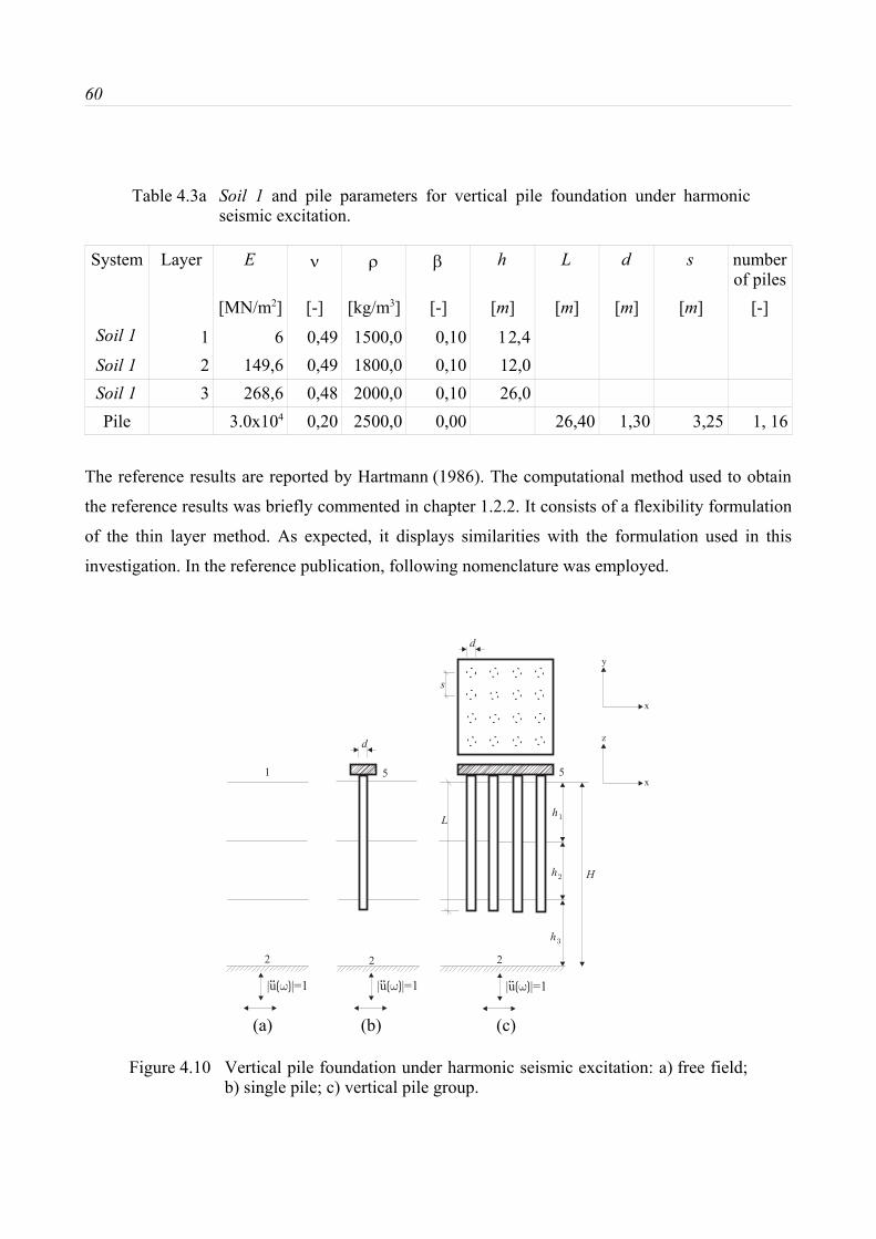
60
Table 4.3a Soil 1 and pile parameters for vertical pile foundation under harmonicseismic excitation.
System Layer E ν ρ β h L d s numberof piles
[MN/m2] [-] [kg/m3] [-] [m] [m] [m] [m] [-]Soil 1 1 6 0,49 1500,0 0,10 12,4
Soil 1 2 149,6 0,49 1800,0 0,10 12,0Soil 1 3 268,6 0,48 2000,0 0,10 26,0Pile 3.0x10⁴ 0,20 2500,0 0,00 26,40 1,30 3,25 1, 16
The reference results are reported by Hartmann (1986). The computational method used to obtain
the reference results was briefly commented in chapter 1.2.2. It consists of a flexibility formulation
of the thin layer method. As expected, it displays similarities with the formulation used in this
investigation. In the reference publication, following nomenclature was employed.
s
d
Lh�
h�
h�
H
d
|u |=1( )�..
|u |=1( )�..
|u |=1( )�..
1
2 2 2
5 5x
z
x
y
(a) (b) (c)
Figure 4.10 Vertical pile foundation under harmonic seismic excitation: a) free field;b) single pile; c) vertical pile group.

4. Implementation of the computational procedure 61
The transfer function from rock to the free surface u1 x / u2 x is defined as the ratio of the
acceleration amplitude at the free surface u1 x to the acceleration amplitude at the rock base
u2 x . The transfer function from rock to the pile cap u5 x / u2 x is defined as the ratio of the
acceleration amplitude at the pile cap u5 x to the acceleration amplitude at the rock base u2 x .
The transfer functions are computed and displayed as a function of the excitation frequency. The
results are compared with the reference results in figure 4.11.
Figure 4.11 Horizontal harmonic foundation top response functions under harmonic
seismic excitation: top: soil 1; bottom: soil 2.
The results obtained from this example match quite good with the reference results. Although the
inertial effects are small because only the mass of the piles is considered, the soil deposit effects
u1 x / u2 x
u5 x / u2 x
u1 x / u2 x
u5 x / u2 x

62
represent a strong component in the dynamic stiffness of the system, as can be seen in the response
functions of the free field. The influence of the piles on the amplitudes of the transfer functions is
higher for the soft soil 1, than for the stiff soil 2. In the latter, little difference can be detected
between the transfer function for a single pile and that for the free surface.
Table 4.3b Soil 2 and pile parameters for vertical pile foundation under harmonicseismic excitation.
System Layer E ν ρ β h L d s numberof piles
[MN/m2] [-] [kg/m3] [-] [m] [m] [m] [m] [-]Soil 2 1 30 0,49 1500,0 0,06 12,4
Soil 2 2 343,3 0,49 1800,0 0,04 12,0Soil 2 3 652,5 0,48 2000,0 0,05 26,0Pile 3.0x10⁴ 0,20 2500,0 0,00 26,40 1,30 3,25 1, 16
4.4 Summary
The validation of the three different examples, namely dynamic stiffness of vertical pile
foundations under harmonic force excitation, dynamic stiffness of vertical and inclined pile
foundations under harmonic force excitation, and transfer functions of vertical pile foundations
under harmonic wave propagation shows that the numerical model with the discretization criteria
employed are able to reproduce the dynamic behavior of single piles and pile groups, with vertical
and/or inclined configurations, in homogeneous halfspaces and in horizontally stratified media.

5. Free field response 63
5. Free field response
This chapter illustrates the seismic free field response analysed according to chapter 3.4.2 through a
particular case example. This example will be used for the seismic soil-structure interaction in the
next chapters of this dissertation. First, a soil deposit and a seismic environment are chosen. The
transfer functions due to wave propagation are computed as explained in chapter 3.4.2.1. Then, an
acceleration history is chosen as seismic excitation. Finally, acceleration time histories due to
seismic excitation are computed as stated in chapter 3.4.2.2.
5.1 Transfer functions due to vertical wave propagation
5.1.1 SV-wave propagation
A soft soil deposit overlaying a rigid rock basin is analysed. The model configuration is displayed
in figure 5.1 with parameters listed in table 5.1. It is assumed that the base rock is rigid and
undergoes a horizontal motion, inducing the free field motion in the overlaying soil deposit. The
free field consists in this case of vertically propagating SV-waves.
8
8H Soil layer
free surface
rigid base
1
2
x
z
|u ( )|=1�2x
..
SV-wave
Figure 5.1 Free field under vertically propagating SV-wave.
The natural frequencies of the soil deposit in shear (induced deformations in x-direction), fnxd, is
computed through equation (2-7):
f n xd =
2 n1cs
4 H
The first modal frequency, f1xd, is than:
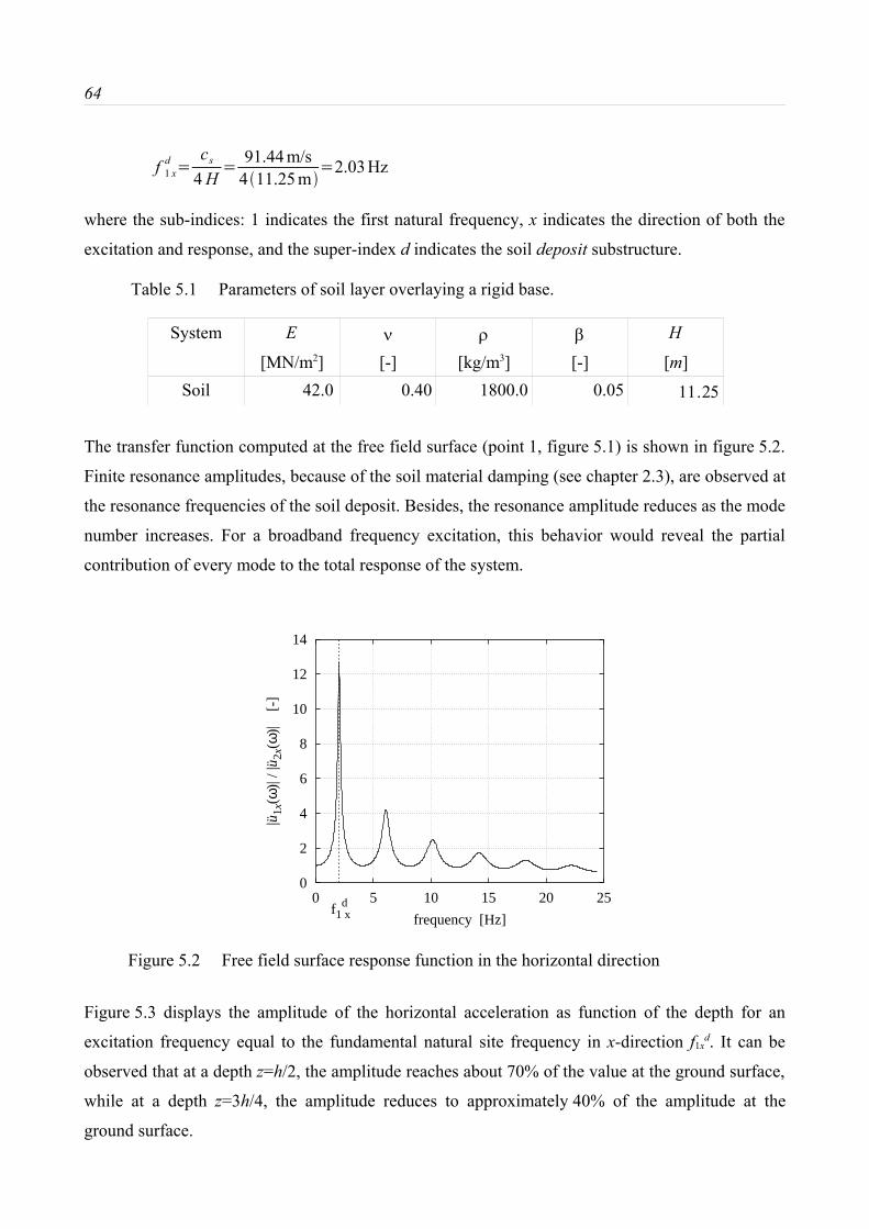
64
f 1 xd =
cs
4 H= 91.44 m/s
411.25 m=2.03 Hz
where the sub-indices: 1 indicates the first natural frequency, x indicates the direction of both the
excitation and response, and the super-index d indicates the soil deposit substructure.
Table 5.1 Parameters of soil layer overlaying a rigid base.
System E ν ρ β H
[MN/m2] [-] [kg/m3] [-] [m]Soil 42.0 0.40 1800.0 0.05 11.25
The transfer function computed at the free field surface (point 1, figure 5.1) is shown in figure 5.2.
Finite resonance amplitudes, because of the soil material damping (see chapter 2.3), are observed at
the resonance frequencies of the soil deposit. Besides, the resonance amplitude reduces as the mode
number increases. For a broadband frequency excitation, this behavior would reveal the partial
contribution of every mode to the total response of the system.
Figure 5.2 Free field surface response function in the horizontal direction
Figure 5.3 displays the amplitude of the horizontal acceleration as function of the depth for an
excitation frequency equal to the fundamental natural site frequency in x-direction f1xd. It can be
observed that at a depth z=h/2, the amplitude reaches about 70% of the value at the ground surface,
while at a depth z=3h/4, the amplitude reduces to approximately 40% of the amplitude at the
ground surface.
0
2
4
6
8
10
12
14
0 5 10 15 20 25
|u1x
(ω)|
/ |u 2
x(ω
)|
[-]
frequency [Hz]
f d1 x

5. Free field response 65
-1
-0.8
-0.6
-0.4
-0.2
0
0 2 4 6 8 10 12 14
z / h
[
-]
|ux(z)| / |u2x| [-]
Figure 5.3 Development of the amplitude of the horizontal acceleration as functionof the depth for an excitation frequency equal to the fundamental soildeposit natural frequency f1x
d.
5.1.2 P-wave propagation
A soft soil deposit overlaying a rigid rock basin is analysed. The model configuration is displayed
in figure 5.4 with parameters listed in table 5.1. It is assumed that the base rock is rigid and
undergoes a vertical motion, inducing the free field motion in the overlaying soil deposit. The free
field consists in this case of vertically propagating P-waves.
The natural frequencies of the soil deposit in compression (induced deformations in z-
direction), fnzd, is computed through equation (2-7) substituting cs through cp :
f nzd =
2 n1c p
4 H

66
8
8H Soil layer
free surface
rigid base
1
2
x
z
|u ( )|=1�2z
..
P-wave
Figure 5.4 Free field under vertically propagating P-wave.
The first eigenfrequency is obtained for n=1 as:
f 1 zd =
c p
4 H= 224 m/s
4 11.25 m=4.98 Hz
The transfer function computed at the free field surface (point 1, figure 5.4) is shown in figure 5.5.
Figure 5.5 Free field surface response function in the vertical direction
A comparison with figure 5.2 indicates that the same resonance amplitudes are calculated for both
horizontal and vertical directions, due to the uncoupled nature of vertical propagation of P- and S-
waves (chapter 2.3). However as the resonance frequencies in x- and z-directions depend from cs
and cp, respectively, the horizontal resonance frequencies are lower than the vertical resonance
0
2
4
6
8
10
12
14
0 5 10 15 20 25
|u1z
(ω)|
/ |u 2
z(ω
)|
[-]
frequency [Hz]
f d1z

5. Free field response 67
frequencies.
5.2 Selection of the input earthquake motion
According to the characteristics of recorded earthquakes, Newmark & Rosenblueth (1971) classify
them into four groups:
1. Practically a single shock. Motions of this type occur only at short distances from the epicenter,
only on firm ground, and only for shallow earthquakes.
2. A moderately long, extremely irregular motion. It is associated with moderate distances from the
focus and occurs only on firm ground. These motions have nearly "white noise" frequency
content. They are ordinarily of almost equal severity in all directions.
3. A long ground motion exhibiting pronounced prevailing periods of vibration. Such motions
result from the filtering of earthquakes of the preceding type through layers of soft soils within
the range of linear or almost linear soil behavior and from the successive wave reflections at the
interfaces of these layers.
4. A ground motion involving large-scale, permanent deformations of the ground. At the site of
interest there may be slides or soil liquefaction.
From the characteristics of the soil configuration and the seismic environment already defined for
this particular example as well as from the assumption of linear behavior, it is evident that the input
motion transmitted from the rock base to the soil deposit should be included in the second group of
the previous classification, namely a nearly white noise motion.
A strict white noise motion is seldom recorded, because particular geological and geophysical
processes modify a seismic motion, before it reaches a soil deposit (chapter 2). In case of a
hypothetic location, like the one currently analysed, the estimation of such influences is unrealistic.
Therefore, a synthetic acceleration history instead of a real seismic record is used in this
investigation.
The artificial acceleration history is generated according to the recommendations of Clough &
Penzien (1993). No specified design response spectrum is employed. The time signal is generated
through random numbers with a Gaussian distribution characterized by a zero mean value and a
variance of unity. According to the typical recorded earthquakes and structural configurations, the
frequency range of interest is chosen between 0.12 and 25.0 Hz. The time history is filtered with a
digital finite impulse response bandpass filter (Rabiner & Gold 1975). A mean uniform amplitude
of the Fourier amplitude spectrum and a maximum acceleration amplitude in the time-domain

68
of 1 m/s2 are assumed. A base line correction is made (Meskouris 2000). The transformation
between time- and frequency-domain and vice versa is achieved through the fast Fourier
transformation and the inverse fast Fourier transformation, respectively. The characteristic values
are listed in table 5.2 (for nomenclature see chapter 4.2.1).
Table 5.2 Characteristic values of simulated acceleration time history.
time-domain frequency-domainN Lz n ∆t Tt ü(t)max ∆f fmin fmax fsa
[-] [-] [-] [s] [s] [m/s2] [Hz] [Hz] [Hz] [Hz]2048 2048 4096 0.02 81.92 1.00 0.0122 0.12 25.00 50.00
The Fourier amplitude spectrum and the time history of the simulated accelerogram are displayed
in figure 5.6, where the arrow indicates the value of the maximum amplitude in the acceleration
time history.
0.0
0.5
1.0
1.5
2.0
2.5
3.0
3.5
4.0
4.5
0 5 10 15 20 25
|u2(
ω)|
[m
/s2 /H
z]
frequency [Hz]
(a)
-2.0
-1.0
0.0
1.0
2.0
0 10 20 30 40 50 60 70 80
u 2(t
) [
m/s
2 ]
time [s]
(b)
1.00
Figure 5.6 Simulated acceleration history: a) Fourier amplitude spectrum; b) time history.

5. Free field response 69
5.3 Vertical wave propagation due to earthquake excitation
5.3.1 SV-wave propagation
The generated acceleration history is prescribed on the rigid base as a vertical propagating SV-
wave. The free field horizontal acceleration history on the ground surface is computed according to
equation (3-15) and exhibited in figure 5.7.
The corresponding Fourier horizontal amplitude spectra is displayed in figure 5.7a. The filtering
effect of the soil layer can be seen comparing figures 5.6a and 5.7a. The corresponding horizontal
accelerogram at the free field surface is exhibited in figure 5.7b. The seismic amplification of the
incoming acceleration time history can be observed. The maximum horizontal amplitude at the
ground surface reaches 205% of the amplitude at the rigid base.
0.0
0.5
1.0
1.5
2.0
2.5
3.0
3.5
4.0
4.5
0 5 10 15 20 25
|u1x
(ω)|
[m
/s2 /H
z]
frequency [Hz]
(a)
-2.0
-1.0
0.0
1.0
2.0
0 5 10 15 20 25 30 35 40
u 1x(
t)
[m/s
2 ]
time [s]
(b)
-2.05
Figure 5.7 Free field surface horizontal acceleration history: a) Fourier amplitudespectrum; b) time history.
5.3.2 P-wave propagation
The generated acceleration history is prescribed on the rigid base as a vertical propagating P-wave.
The free field vertical acceleration history on the ground surface is computed and exhibited in
figure 5.8.
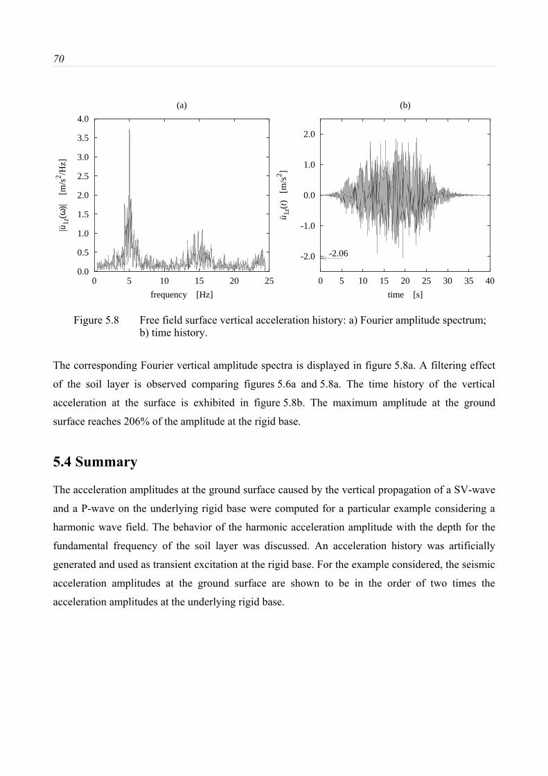
70
0.0
0.5
1.0
1.5
2.0
2.5
3.0
3.5
4.0
0 5 10 15 20 25
|u1z
(ω)|
[m
/s2 /H
z]
frequency [Hz]
(a)
-2.0
-1.0
0.0
1.0
2.0
0 5 10 15 20 25 30 35 40u 1
z(t)
[m
/s2 ]
time [s]
(b)
-2.06
Figure 5.8 Free field surface vertical acceleration history: a) Fourier amplitude spectrum;b) time history.
The corresponding Fourier vertical amplitude spectra is displayed in figure 5.8a. A filtering effect
of the soil layer is observed comparing figures 5.6a and 5.8a. The time history of the vertical
acceleration at the surface is exhibited in figure 5.8b. The maximum amplitude at the ground
surface reaches 206% of the amplitude at the rigid base.
5.4 Summary
The acceleration amplitudes at the ground surface caused by the vertical propagation of a SV-wave
and a P-wave on the underlying rigid base were computed for a particular example considering a
harmonic wave field. The behavior of the harmonic acceleration amplitude with the depth for the
fundamental frequency of the soil layer was discussed. An acceleration history was artificially
generated and used as transient excitation at the rigid base. For the example considered, the seismic
acceleration amplitudes at the ground surface are shown to be in the order of two times the
acceleration amplitudes at the underlying rigid base.

6. Soil-foundation interaction 71
6. Soil-foundation interaction
6.1 Introduction
Considering the decrease of the acceleration amplitude with increasing depth at the free field (see
figure 5.3), it is observed that a deep foundation system is exposed at its lower end to an input
amplitude lower than the amplitude at the ground surface. The dynamic behavior as well as the
amplitude expected at the top of the foundation (without considering any structure on it), will
depend on the stiffness ratio between foundation and subsoil. On the opposite, a surface foundation
experiences an input acceleration amplitude equal to the acceleration amplitude at the ground
surface.
In this chapter, the soil-foundation interaction is analysed as described in chapter 3.4.2.1. No
superstructure is considered at this stage. A schematic configuration of the analysed system is
displayed in figure 6.1. The response is computed as transfer functions at all nodes. Attention is
paid to the ratio ü5ω/ü1ω between the transfer functions computed at the top of the foundation
(point 5), and the transfer functions at the free surface of the soil deposit model (point 1), computed
in section 5.1.
(a) (b)
Figure 6.1 System configuration under harmonic base rock excitation: a) Free fieldsystem; b) Soil-foundation system.
Three foundation types are investigated: rigid surface foundation, pile foundation and soil
improvement foundation (volume of soil improvement underlaying rigid surface foundations). All
1
2
rigid base
body waves
5
2
4
x
z
free surface free surface
rigid base
body waves
soil layer soil layer
foundation
8H
8

72
three foundation types have a square cross-section at the ground surface level. The ability of the
foundation to experience acceleration amplitudes at the surface level lower than those recorded at
the soil surface for free field is defined as the seismic soil-foundation interaction. The seismic soil-
foundation interaction indicates the foundation contribution to the seismic vibration reduction in
the superstructure.
In order to facilitate comparisons between the foundation types, besides the behavior of the
foundations under seismic excitation, the foundation behavior under an external harmonic load
applied at the foundation top is also simulated. The system response is presented in form of real
components and imaginary components of the dynamic stiffness functions, as defined in
chapter 4.3.2. It has been shown that the dynamic stiffness functions of rigid massless square
foundations resting on elastic halfspaces do not differ much from the dynamic stiffness functions of
rigid massless circular foundations on identical subsoil conditions, if both circle and square have
the same area for the translation movements and the same moment of inertia for rotation
movements (Sieffert & Cevaer 1991). Therefore, the amplitudes of the real components as well as
the amplitudes of the imaginary components are normalized with respect to the static stiffness of a
rigid massless equivalent circular foundation laying on a homogeneous elastic halfspace. These
values can be calculated analytically. In Richart & Woods (1970), following expressions are given:
k xxc= 8Gr
2ν(6-1a)
kψψc = 8Gr3
31ν(6-1b)
k zzc= 4Gr
1ν(6-1c)
where kxxc, kψψ
c and kzzc are the static stiffnesses of a rigid massless circular surface foundation
laying on an isotropic halfspace in the translational x-, rotational yy-, and translational z-direction
respectively, G is the soil shear modulus, r is the foundation radius and ν is the Poisson's ratio. In
this context, a dimensionless frequency is defined as:
a0=ω rcs
(6-2)
where ω is the excitation circular frequency and cs the S-wave propagation velocity of the soil.

6. Soil-foundation interaction 73
The radius of the equivalent circular foundation is calculated assuming the same plane area as the
foundations of square cross-section for the cases of x- and z-translational excitations, and assuming
the same second moment of inertia as the foundations of square cross-section for the case of a ψ-
rotational excitation.
6.2 Discretization of the model
The investigated systems are discretized with the criteria described in chapter 4.2.2. Examples of
typical physical and discrete models are exhibited in figures 6.2, 6.3 and 6.4.
soil layers
simulated half-space
plateelements
2B
2B
t
x
z
x
y
(a) (b) (c)(a) (b) (c)
Figure 6.2 Typical surface foundation configuration: a) physical model; b) discretesoil deposit model; c) discrete structural model.
6.3 Surface foundation
Transfer functions due to harmonic base rock excitation
The analysed problem is displayed in figure 6.5. The geometrical and mechanical parameters are
listed in table 6.1. It corresponds to the following configuration:
• Subsoil configuration: homogeneous damped elastic layer over rigid base (layer over rigid base)

74
2B
2B
s
s
s s
dt
Lembedment
additional soil layers
simulated half-space
thin layersbeamelements
plateelements
x
z
x
y
(a) (b) (c)(a) (b) (c)
Figure 6.3 Typical pile group configuration: a) physical model; b) discrete soildeposit model; c) discrete structural and excavated soil model.
2B
2B
L
plate elements
volumeelements
2b
2b
thin layers
embedment
additional soil layers
simulated half-space
x
z
x
y
(b)(a) (c)
Figure 6.4 Typical soil improvement foundation configuration: a) physical model; b)discrete soil deposit model; c) discrete structural and excavated soilmodel.

6. Soil-foundation interaction 75
• Rigid massless surface foundation
• Support excitations at the rigid base in different directions:
a) Horizontal direction: upward vertical propagating SV-wave
Vertical direction: upward vertical propagating P-waveA relatively high elastic modulus is
assigned to the foundation in order to simulate its rigid behavior.
H
2B
2B
x
z
x
y
|u |=1( )�..
2
5
Figure 6.5 Rigid massless surface foundation under harmonic base rock excitation.
The ratio of transfer functions ü5ω/ü1ω (see figure 6.1) for the case of upward vertical
propagating SV-wave and for the case of upward vertical propagating P-wave are displayed in
figure 6.6a and figure 6.6b respectively. It can be seen that in both cases the amplitude of the
response at the foundation does not differ from the amplitude of the response of the free field at the
soil surface. No seismic soil-foundation interaction is observed.
Table 6.1 Surface foundation on layer over rigid base. Mechanical and geometricparameters.
System E ν ρ β H 2B
[MN/m2] [-] [kg/m3] [-] [m] [m]soil 42.0 0.40 1800.0 0.05 11.25
foundation ∞ - 0.0 0.00 1.80
Assuming a 2-dimensional state, points located on the same horizontal layer display the same
vibration amplitude for the free field condition, ∣δ∣ (see section 3.3.2), but different phase

76
angles depending on their locations. A rigid surface foundation forces a vibration in phase of the
soil-foundation interface, but is not able to modify the vibration amplitude.
0
0.2
0.4
0.6
0.8
1
1.2
1.4
0 5 10 15 20 25
|u5x
(ω)|
/ |u 1
x(ω
)|
[-]
frequency [Hz]
(a)
0
0.2
0.4
0.6
0.8
1
1.2
1.4
0 5 10 15 20 25
|u5z
(ω)|
/ |u 1
z(ω
)|
[-]
frequency [Hz]
(b)
Figure 6.6 Surface foundation. Ratio of transfer functions ü5ω/ü1ω : a) verticalpropagating SV-wave; b) vertical propagating P-wave.
Harmonic load excitation at the foundation
The analysed problem is displayed in figure 6.7. The geometrical and mechanical parameters are
listed in table 6.1. It corresponds to the following configuration:
H
2B
2B
2B
2B
|F |=1( )�|F |=1( )�
x
z
x
y
(b)(a)
Figure 6.7 Rigid massless surface foundation under harmonic load: a) layer overrigid base; b) halfspace.

6. Soil-foundation interaction 77
0
0.2
0.4
0.6
0.8
1
1.2
1.4
1.6
0 0.2 0.4 0.6 0.8 1 1.2 1.4 1.6
k xx
/ kc xx
[-]
a0 [-]
(a)
halfspacelayer over rigid base
0
0.2
0.4
0.6
0.8
1
1.2
1.4
1.6
0 0.2 0.4 0.6 0.8 1 1.2 1.4 1.6
c xx
/ kc xx
[-]
a0 [-]
(b)
halfspace layer over rigid base
0
0.2
0.4
0.6
0.8
1
1.2
1.4
1.6
0 0.2 0.4 0.6 0.8 1 1.2 1.4 1.6
k ψψ
/ kc ψ
ψ
[-
]
a0 [-]
(c)
halfspacelayer over rigid base
0
0.2
0.4
0.6
0.8
1
1.2
1.4
1.6
0 0.2 0.4 0.6 0.8 1 1.2 1.4 1.6
c ψψ
/ kc ψ
ψ
[-
]
a0 [-]
(d)
halfspace layer over rigid base
0
0.2
0.4
0.6
0.8
1
1.2
1.4
1.6
0 0.2 0.4 0.6 0.8 1 1.2 1.4 1.6
k zz
/ kc zz
[-]
a0 [-]
(e)
halfspacelayer over rigid base
0
0.2
0.4
0.6
0.8
1
1.2
1.4
1.6
0 0.2 0.4 0.6 0.8 1 1.2 1.4 1.6
c zz
/ kc zz
[-]
a0 [-]
(f)
halfspacelayer over rigid base
Figure 6.8 Dynamic stiffness functions of surface square foundation under harmonic loadexcitation at foundation top: a) real component in x-direction; b) imaginary componentin x-direction; c) real component in yy-direction; d) imaginary component in yy-direction; e) real component in z-direction; f) imaginary component in z-direction.

78
• Two subsoil configurations:
a) Homogeneous damped elastic layer over rigid base (layer over rigid base)
b) Homogeneous damped elastic halfspace (halfspace)
• rigid massless plate, laying on the ground surface
• Different harmonic load excitations at the foundation:
a) Force in x-direction
b) Moment in y-direction
c) Force in z-direction
For the geometric and mechanical parameters of the current soil-foundation system, the evaluation
of the static stiffnesses of a rigid massless equivalent circular surface foundation laying on a
homogeneous elastic halfspace gives (equations 4-1a, 4-1b and 4-1c respectively):
k xxc=8G r
2ν= 81.51 x 10⁷ N /m21.016 m
20.4=7.66 x 10⁷ N /m2
kψψc = 8G r3
31ν= 81.51 x 10⁷ N /m21.008 m3
310.4=6.86 x 10⁷ N /m2
k zzc= 4G r
1ν= 41.51 x 10⁷ N /m21.016 m
10.4=1.02 x 10⁸ N /m2
These are the reference values used for the normalization of the real and imaginary components of
the dynamic stiffness functions. The normalized real and imaginary components are displayed in
figure 6.8 for excitations defined in the horizontal, rotational and vertical direction.
For the static case, a very good agreement is obtained between the results computed and the
reference values from equations (6-1a) and (6-1c) for translational excitations in x- and z-direction,
respectively. The static normalized real component of the dynamic stiffness function for a
rotational excitation shown in figure 6.8 is found to be about 0.85. According to Kausel (2002),
such result is related with the particular definition of the mean rotation inside of flexible loaded
disk acting on the surface of a homogeneous halfspace (Kausel & Peek 1982), which differs with
the particular definition of the mean rotation inside of a rigid loaded disk acting on the surface of a
homogeneous halfspace (Richart & Woods 1970) in a factor of 0.868.
For the case halfspace and for all three directions of the excitation, the real components of the
dynamic stiffness function decrease with increasing frequency. The imaginary components of the
dynamic stiffness functions increase with increasing frequency. The inconsistency of the linear
hysteretic damping formulation (see chapter 3) is observed with a "static damping" value. The

6. Soil-foundation interaction 79
increase of the imaginary component of the dynamic stiffness function with the frequency indicates
the so-called radiation damping phenomena (Siefert & Cevaer 1991, Chouw 1994).
For the case layer over rigid base, the presence of the rigid boundary below the model and its
consequent wave reflection explains that: On the one side, the real component display some
waviness for excitations specified in the horizontal and vertical direction, specially for low
frequencies; on the other side, the imaginary component displays a constant value for frequencies
lower than the fundamental soil deposit natural frequency. This constant damping amplitude revels
that for frequencies lower than the fundamental soil deposit natural frequency, no radiation
damping (wave propagation to the infinity) occurs. Therefore, the fundamental soil deposit natural
frequency is known as cut-off frequency (Waas 1972, Chouw 1994).
6.4 Pile foundations
6.4.1 Single piles
Transfer functions due to harmonic base rock excitation
The analysed problem is displayed in figure 6.9. The geometrical and mechanical parameters are
listed in table 6.2. It corresponds to the following configuration:
�
d
HL
|u |=1( )�..
x
z
x
y
2
5
Figure 6.9 Single pile under base rock excitation
Table 6.2 Single pile in soil layer over rigid base. Mechanical and geometricparameters.

80
System E ν ρ β H L d number of piles
α
[MN/m2] [-] [kg/m3] [-] [m] [m] [m] [-] [°]Soil 42 0.40 1800.0 0.05 11.25
Pile 4.2x10⁴ 0.25 2500.0 0.00 9.00 0.60 1 variable
• Subsoil configuration: homogeneous damped elastic layer over rigid base (layer over rigid base)
• Single pile rigidly connected to the cap
• Rigid massless pile cap, without contact with the ground surface
• Different pile inclinations with respect to the z-axis in the plane x-z:
a) α = 0°
b) α = 33.7°
c) α = 53.1°
d) α = 63.4°
• Support excitations at the rigid base in different directions::
a) Upward vertical propagating SV-wave
b) Upward vertical propagating P-wave
The ratio of transfer functions ü5ω/ü1ω (see figure 6.1) for the case of upward vertical
propagating SV-wave and for the case of upward vertical propagating P-wave are displayed in
figure 6.10a and figure 6.10b respectively.
In figure 6.10a, it can be seen that a vertical pile (α=0°) display the same response amplitude as
that of soil surface for free field conditions for frequencies lower than about 3 Hz (which is also
higher than the first natural frequency of the site f1xd in x-direction ). For higher frequencies,
considerable reductions in the transfer functions are observed. Due to the usually amplification that
a soft soil surface layer produces in a seismic excitation for low frequencies (Romo et al., 2000,
Waas 1989, Chouw 1994), it can be supposed that a single vertical pile would experience almost
the same acceleration amplitudes as the free field.

6. Soil-foundation interaction 81
0
0.2
0.4
0.6
0.8
1
0 5 10 15 20 25
|u5x
(ω)|
/ |u 1
x(ω
)|
[-]
frequency [Hz]
(a)
f d1x
α= 0.0° α=33.7°α=53.1°α=63.4°
0
0.2
0.4
0.6
0.8
1
0 5 10 15 20 25|u
5z(ω
)| / |
u 1z(
ω)|
[-
]frequency [Hz]
(b)
f d1z
α= 0.0°α=33.7°α=53.1°α=63.4°
Figure 6.10 Single pile. Ratio of transfer functions ü5ω/ü1ω : a) vertical propagatingSV-wave; b) vertical propagating P-wave.
Next, the influence of the inclination of the pile with respect to the z-axis is evaluated. The inclined
pile tips also reach the same depth z=-9.0 m, that implies a length as function of the inclination. It
can be observed, that the inclination of the pile induces a contribution in the acceleration reduction
at the pile head, namely the ratio of transfer functions ü5ω/ü1ω shows an amplitude reduction
starting at lower frequencies than the first natural frequency of the soil deposit. For a horizontal
excitation, with increasing inclination, an increasing reduction at the ratio of response function in
particular in the frequeny range of 0-10 Hz can be observed. This behavior stabilizes for an
inclination about α=63.4°. In this range, the head of an inclined pile experiences lower horizontal
acceleration amplitudes than the accelerations amplitudes at the soil surface for free field.
In figure 6.10b, it can be seen that a vertical pile (α=0°) experiences a reduction of the vertical
acceleration amplitude with respect to the vertical acceleration amplitude at the free field for
increasing frequencies. This amplitude reduction starts at a very low frequency. At a frequency
about 5 Hz, which is the first natural frequency of the soil deposit in the vertical direction f1zs, the
vertical acceleration amplitude at the pile head is about 70% the vertical acceleration amplitude at
the free field surface. At a frequency about 15 Hz, which is the second natural frequency of the site
in the vertical direction, the vertical acceleration amplitude at the pile head is about 25% the
vertical acceleration amplitude of the free field at the soil surface. That means, a single vertical pile
under a vertical harmonic excitation would experience lower vertical acceleration amplitudes on

82
the pile head, than the vertical acceleration amplitudes for free field at the soil surface.
The inclination of a single pile with respect to the z-axis has the opposite effect in the vertical
transfer function than that in the horizontal transfer function, namely the vertical acceleration
amplitudes at the pile head tends to those of the free field with increasing inclination. This situation
may be attributed to the inertial effects due to the pile mass, which increases with the length of the
pile.
Due to the opposite effect of the inclination of the pile in the horizontal and vertical harmonic
vibration reduction at the pile head, a compromise should be taken to fulfill a satisfactory behavior
for both directions of the excitation. In a frequency range of 0 up to about 5 Hz, the reduction in the
horizontal direction is more pronounced than the amplification in the vertical direction. Therefore,
in the case of a mixed seismic excitation with equal horizontal and vertical amplitudes, an
inclination of 53.1° would be well suited in order to reduce the acceleration amplitude at the
foundation top at the first natural frequency of the soil deposit in horizontal direction as well as at
the first natural frequency of the soil deposit in vertical direction.
6.4.2 Pile groups
6.4.2.1 Vertical pile groups
Transfer functions due to harmonic base rock excitation
The analysed problem is displayed in figure 6.11. The geometrical and mechanical parameters are
listed in table 6.3. It corresponds to the following configuration:
• Subsoil configuration: homogeneous damped elastic layer over rigid base (layer over rigid base)
• 2x2 vertical pile group rigidly connected to the cap
• rigid massless pile cap laying on the ground surface
• Different pile spacings:
a) s/d=2
b) s/d=4
c) s/d=6
d) s/d=8
e) s/d=10
• Support excitations at the rigid base in different directions::

6. Soil-foundation interaction 83
a) Upward vertical propagating SV-wave
b) Upward vertical propagating P-wave
A
A´'
� �
LH
Section A-A'
s
d
|u |=1( )�..
x
y
2
5
d
Figure 6.11 Pile group under base rock excitation.
The ratio of transfer functions ü5ω/ü1ω (see figure 6.1) for the case of upward vertical
propagating SV-wave and for the case of upward vertical propagating P-wave are displayed in
figure 6.12a and figure 6.12b respectively. For comparison, the results for a single vertical pile are
also shown.
Table 6.3 Vertical pile group in soil layer over rigid base. Mechanical and geometricparameters.
System E ν ρ β H L d s number of piles
α
[MN/m2] [-] [kg/m3] [-] [m] [m] [m] [m] [-] [°]Soil 42 0.40 1800.0 0.05 11.25
Pile 4.2x10⁴ 0.25 2500.0 0.00 9.00 0.60 variable 4 0.00
In figure 6.12a, it can be seen that the ratio of horizontal response functions of a pile group with
very low pile spacing is very similar to that of a single pile. For frequencies lower than 3 Hz, little
influence of the pile spacing is observed. This includes the soil deposit first horizontal natural
frequency at about f1xd = 2 Hz. For frequencies higher than 3 Hz, an increase in the pile spacing
reduces the contribution of the pile group to the vibration reduction with increasing frequencies.
This indicates a reduction of the horizontal foundation effectiveness with an increasing pile spacing
for high frequencies.

84
0
0.2
0.4
0.6
0.8
1
0 5 10 15 20 25
|u5x
(ω)|
/ |u 1
x(ω
)|
[-]
frequency [Hz]
(a)
f d1x
single piles/d=2s/d=4s/d= 6s/d= 8
s/d=10
0
0.2
0.4
0.6
0.8
1
0 5 10 15 20 25|u
5z(ω
)| / |
u 1z(
ω)|
[-
]frequency [Hz]
(b)
f d1z
single piles/d= 2s/d= 4s/d= 6s/d= 8s/d=10
Figure 6.12 Vertical pile group. Ratio of transfer functions ü5ω/ü1ω : a) verticalpropagating SV-wave; b) vertical propagating P-wave.
In figure 6.12b, it can be seen that the ratio of vertical response functions of pile groups with very
low pile spacing is very similar to that of a single pile. For frequencies lower than 3 Hz, little
influence of the pile spacing is observed. For frequencies higher than 3 Hz, an increase in the pile
spacing reduces the contribution of the pile group to the vibration reduction with increasing
frequencies. For the soil deposit first vertical natural frequency f1zs, about 5 Hz, the amplitude of the
ratio of vertical response function oscillates between 66% for a pile spacing s/d=2 and 76% for a
pile spacing s/d=10. A reduction of the foundation effectiveness with an increasing pile spacing for
high frequencies is observed.
Harmonic load excitation at the pile cap
The analysed problem is displayed in figure 6.13. The geometrical and mechanical parameters are
listed in table 6.3. It corresponds to the following configuration:
• Two subsoil configurations:
a) Homogeneous damped elastic layer over rigid base (layer over rigid base)
b) Homogeneous damped elastic halfspace (halfspace)
• 2x2 vertical pile group rigidly connected to the cap with pile spacing s/d=2
• rigid massless pile cap laying on the ground surface
• Different harmonic load excitations at the foundation:

6. Soil-foundation interaction 85
a) Force in x-direction
b) Moment in y-direction
c) Force in z-direction
A
A´'
� � L
Section A-A'
s
A
A´'
� �
LH
Section A-A'
s
d d|F |=1( )� |F |=1( )�
x
y
(b)(a)
Figure 6.13 Pile group under harmonic load excitation at foundation top: a) layerover rigid base; b) halfspace.
The normalized real and imaginary components of the dynamic stiffness functions are displayed in
figure 6.14 for excitations defined in the horizontal, rotational and vertical direction. Despite the
coupling between the translational horizontal and the rotational rocking stiffness, the horizontal
stiffness is computed considering the pile head yy-rotation constrained and the rocking stiffness is
computed considering the pile head x-displacement constrained. These are compared with
figure 6.8 for a rigid surface foundation with the same cross-section.
For the case halfspace, the ratio between the static stiffness component of the vertical pile group
and the static stiffness component of the surface foundation is:
• for a x-translational excitation about 2.5;
• for a yy-rotational excitation about 22; and,
• for a z-translational excitation about 3.5.

86
0
2
4
6
8
10
0 0.2 0.4 0.6 0.8 1 1.2 1.4 1.6
k xx
/ kc xx
[-]
a0 [-]
(a)
halfspacelayer over rigid base
0
2
4
6
8
10
12
0 0.2 0.4 0.6 0.8 1 1.2 1.4 1.6
c xx
/ kc xx
[-]
a0 [-]
(b)
halfspacelayer over rigid base
0
5
10
15
20
25
30
35
40
0 0.2 0.4 0.6 0.8 1 1.2 1.4 1.6
k ψψ
/ kc ψ
ψ
[-
]
a0 [-]
(c)
halfspacelayer over rigid base
0
5
10
15
20
25
0 0.2 0.4 0.6 0.8 1 1.2 1.4 1.6
c ψψ
/ kc ψ
ψ
[-
]
a0 [-]
(d)
halfspacelayer over rigid base
-10
-5
0
5
10
0 0.2 0.4 0.6 0.8 1 1.2 1.4 1.6
k zz
/ kc zz
[-]
a0 [-]
(e)
halfspacelayer over rigid base
0
2
4
6
8
10
12
14
16
0 0.2 0.4 0.6 0.8 1 1.2 1.4 1.6
c zz
/ kc zz
[-]
a0 [-]
(f)
halfspacelayer over rigid base
Figure 6.14 Dynamic stiffness functions of vertical pile group under harmonic loadexcitation at foundation top: a) real component in x-direction; b) imaginarycomponent in x-direction; c) real component in yy-direction; d) imaginarycomponent in yy-direction; e) real component z-direction; f) imaginarycomponent in z-direction.

6. Soil-foundation interaction 87
An increase in the static stiffness component of the vertical pile group is observed in comparison
with the static stiffness component of the surface foundation for all three excitation directions. In
the yy-rotational direction, the increment of the static stiffness of the vertical pile group with
respect to the static stiffness of the surface foundation is especially high, which restricts the
deformability in this degree of freedom. Regarding the real components in both x- and z-
translational directions, a higher frequency dependence is observed for the vertical pile group than
for the surface foundation. The imaginary component displays a linear frequency dependence for
all three excitation directions. Higher values are observed for the imaginary component of the
vertical pile group in comparison with the imaginary component of the surface foundation for the
same excitation frequency.
For the case layer over rigid base, a similar behavior is observed as for a surface foundation
(namely on the one side the real component displays a waviness for excitations acting in the
horizontal and vertical direction, specially for low frequencies; and on the other side, it is observed
a constant imaginary component for frequencies lower than the fundamental natural frequency of
the soil deposit) is observed for a vertical pile foundation. Higher values are observed for the
imaginary component of the vertical pile group in comparison with the imaginary component of the
surface foundation for the same excitation frequency.
6.4.2.2 Inclined pile groups
Transfer functions due to harmonic base rock excitation
The analysed problem is displayed in figure 6.11. The geometrical and mechanical parameters are
listed in table 6.4. It corresponds to the following configuration:
• Subsoil configuration: homogeneous layer over rigid base (layer over rigid base)
• 2x2 inclined pile group rigidly connected to the cap
• Pile inclination: α=53.1°
• rigid massless pile cap laying on the ground surface
• Different pile spacings at the pile cap:
a) s/d=2
b) s/d=4
c) s/d=6
d) s/d=8
e) s/d=10
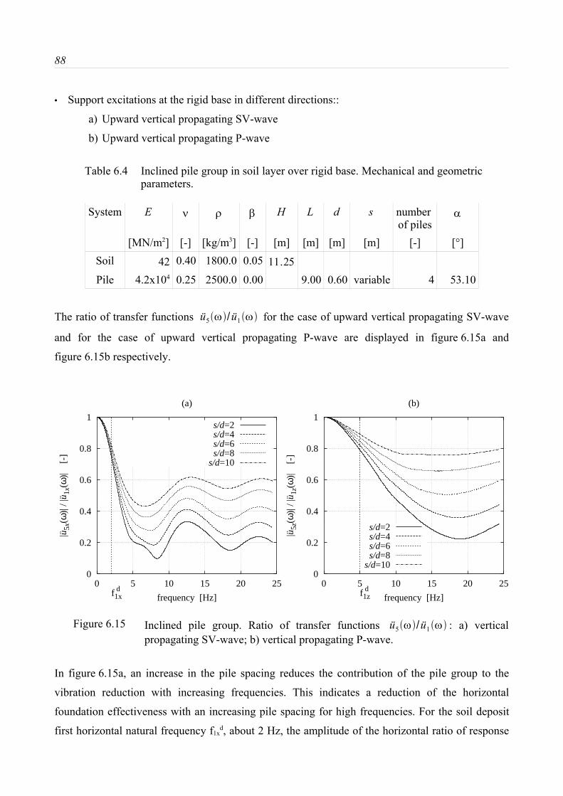
88
• Support excitations at the rigid base in different directions::
a) Upward vertical propagating SV-wave
b) Upward vertical propagating P-wave
Table 6.4 Inclined pile group in soil layer over rigid base. Mechanical and geometricparameters.
System E ν ρ β H L d s number of piles
α
[MN/m2] [-] [kg/m3] [-] [m] [m] [m] [m] [-] [°]Soil 42 0.40 1800.0 0.05 11.25
Pile 4.2x10⁴ 0.25 2500.0 0.00 9.00 0.60 variable 4 53.10
The ratio of transfer functions ü5ω/ü1ω for the case of upward vertical propagating SV-wave
and for the case of upward vertical propagating P-wave are displayed in figure 6.15a and
figure 6.15b respectively.
0
0.2
0.4
0.6
0.8
1
0 5 10 15 20 25
|u5x
(ω)|
/ |u 1
x(ω
)|
[-]
frequency [Hz]
(a)
f d1x
s/d=2s/d=4s/d=6s/d=8
s/d=10
0
0.2
0.4
0.6
0.8
1
0 5 10 15 20 25
|u5z
(ω)|
/ |u 1
z(ω
)|
[-]
frequency [Hz]
(b)
f d1z
s/d=2s/d=4s/d=6s/d=8
s/d=10
Figure 6.15 Inclined pile group. Ratio of transfer functions ü5ω/ü1ω : a) verticalpropagating SV-wave; b) vertical propagating P-wave.
In figure 6.15a, an increase in the pile spacing reduces the contribution of the pile group to the
vibration reduction with increasing frequencies. This indicates a reduction of the horizontal
foundation effectiveness with an increasing pile spacing for high frequencies. For the soil deposit
first horizontal natural frequency f1xd, about 2 Hz, the amplitude of the horizontal ratio of response

6. Soil-foundation interaction 89
function oscillates between 73% for s/d=2 and 81% for s/d=10. For frequencies higher than 3 Hz,
an increase in the pile spacing reduces the contribution of the pile group to the vibration reduction
with increasing frequencies. This indicates a reduction of the horizontal foundation effectiveness
with an increasing pile spacing for high frequencies.
In figure 6.15b, for very low frequencies, between 0 and 1 Hz, little influence of the pile spacing is
observed. For frequencies higher than 1 Hz, an increase in the pile spacing reduces the contribution
of the pile group to the vibration reduction with increasing frequencies. For the soil deposit first
vertical natural frequency f1zd, about 5 Hz, the amplitude of the ratio of vertical response function
oscillates between 78% for a pile spacing s/d=2 and 89% for a pile spacing s/d=10. A reduction of
the foundation effectiveness with an increasing pile spacing for high frequencies is observed.
Harmonic load excitation at the pile cap
The analysed problem is displayed in figure 6.13. The geometrical and mechanical parameters are
listed in table 6.4. It corresponds to the following configuration:
• Two subsoil configurations:
a) Homogeneous layer over rigid base (layer over rigid base)
b) Homogeneous halfspace (halfspace)
• 2x2 inclined pile group rigidly connected to the cap with pile spacing s/d=2 at the pile cap
• Pile inclination with the vertical: α=53.1°
• rigid massless pile cap laying on the ground surface
• Different harmonic load excitations at the foundation:
a) Force in x-direction
b) Moment in y-direction
c) Force in z-direction
The normalized real and imaginary components of the dynamic stiffness functions are displayed in
figure 6.16 for excitations acting in the horizontal, rotational and vertical direction. These are
compared with figure 6.8 for a rigid surface foundation with the same cross-section as the pile cap.
For the case halfspace, the ratio between the static stiffness component of the inclined pile group
and the static stiffness component of the surface foundation is:
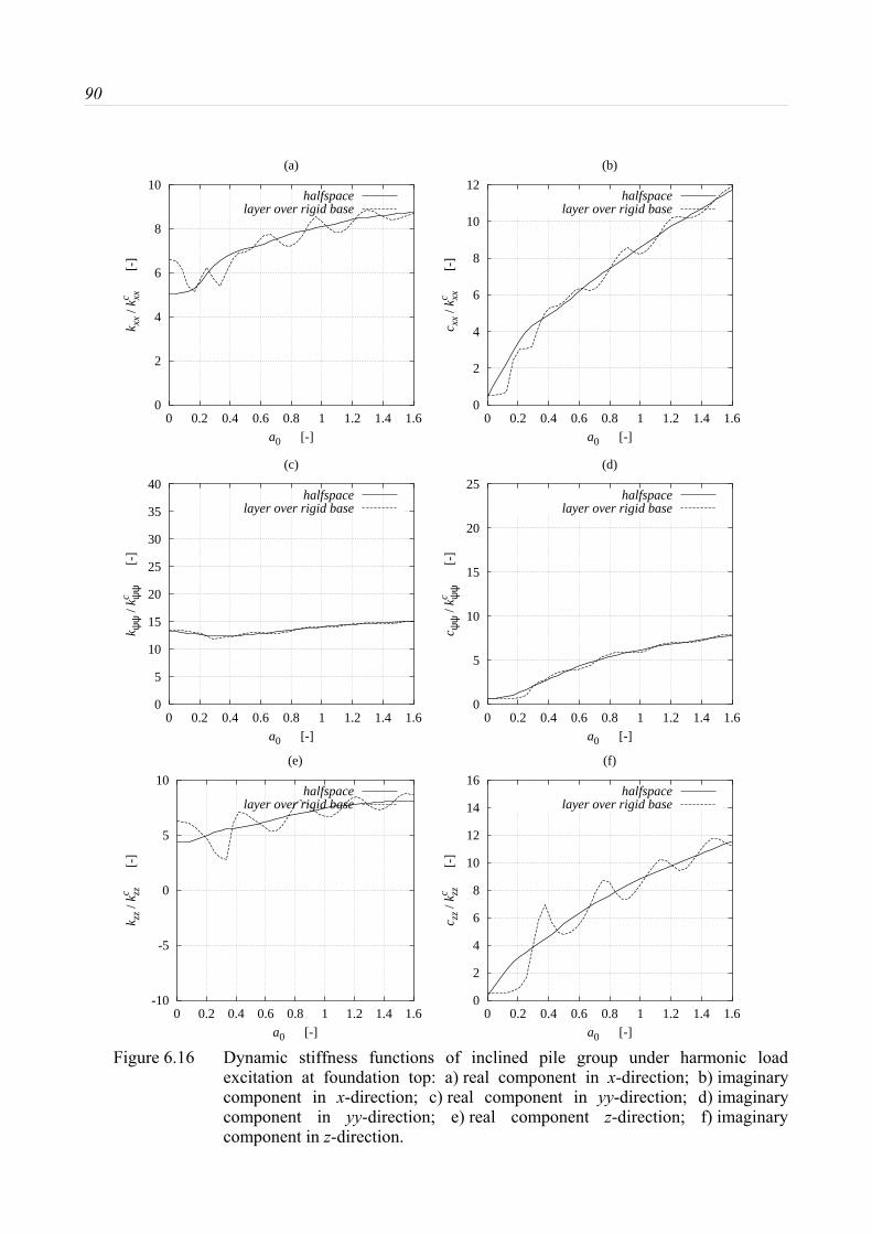
90
0
2
4
6
8
10
0 0.2 0.4 0.6 0.8 1 1.2 1.4 1.6
k xx
/ kc xx
[-]
a0 [-]
(a)
halfspacelayer over rigid base
0
2
4
6
8
10
12
0 0.2 0.4 0.6 0.8 1 1.2 1.4 1.6
c xx
/ kc xx
[-]
a0 [-]
(b)
halfspacelayer over rigid base
0
5
10
15
20
25
30
35
40
0 0.2 0.4 0.6 0.8 1 1.2 1.4 1.6
k ψψ
/ kc ψ
ψ
[-
]
a0 [-]
(c)
halfspacelayer over rigid base
0
5
10
15
20
25
0 0.2 0.4 0.6 0.8 1 1.2 1.4 1.6
c ψψ
/ kc ψ
ψ
[-
]
a0 [-]
(d)
halfspacelayer over rigid base
-10
-5
0
5
10
0 0.2 0.4 0.6 0.8 1 1.2 1.4 1.6
k zz
/ kc zz
[-]
a0 [-]
(e)
halfspacelayer over rigid base
0
2
4
6
8
10
12
14
16
0 0.2 0.4 0.6 0.8 1 1.2 1.4 1.6
c zz
/ kc zz
[-]
a0 [-]
(f)
halfspacelayer over rigid base
Figure 6.16 Dynamic stiffness functions of inclined pile group under harmonic loadexcitation at foundation top: a) real component in x-direction; b) imaginarycomponent in x-direction; c) real component in yy-direction; d) imaginarycomponent in yy-direction; e) real component z-direction; f) imaginarycomponent in z-direction.

6. Soil-foundation interaction 91
• for a x-translational excitation about 5;
• for a yy-rotational excitation about 13; and,
• for a z-translational excitation about 4.4.
The ratio between the static stiffness component of the inclined pile group and the static stiffness
component of the vertical pile group is:
• for a x-translational excitation about 2;
• for a yy-rotational excitation about 0.7; and,
• for a z-translational excitation about 1.3.
An increase in the static stiffness component of the vertical pile group is observed in comparison
with the static stiffness component of the surface foundation for all three excitation directions. In
the yy-rotational direction, the increment of the static stiffness of the vertical pile group with
respect to the static stiffness of the surface foundation is especially high, which restricts the
deformability in this degree of freedom. Regarding the real components in both x- and z-
translational directions, a different frequency dependent behavior is observed for the vertical pile
group than for the surface foundation: the real components of an inclined pile group in both x- and
z-translational directions increase with an increasing frequency. The imaginary component displays
a frequency-dependent behavior for all three excitation directions. Higher values are observed for
the imaginary component of the vertical pile group in comparison with the imaginary component of
the surface foundation for the same excitation frequency.
For the case layer over rigid base, for an excitation in the vertical direction, a higher amplitude
oscillation is observed on the waviness of the real component and of the imaginary component of
the dynamic stiffness functions of the inclined pile group, in comparison with the real component
and of the imaginary component of the dynamic stiffness functions of a surface foundation. Higher
values are observed for the imaginary component of the vertical pile group in comparison with the
imaginary component of the surface foundation for the same excitation frequency.

92
6.5 Soil improvement foundations
6.5.1 Soil improvement foundation equivalent to a vertical pile foundation
A comparison between the harmonic behavior of a soil improvement foundation "equivalent" to a
vertical pile group is presented in this chapter. A block with equivalent parameters to the 2x2
vertical pile group considered in chapter 6.4.2.1 and listed in table 6.5 is analysed. The outer
dimensions, static stiffness and average mass of the pile group and the soil inside are assigned to
the block. Depending on the direction of the excitation, the mechanical parameters are chosen in
order to reproduce the static stiffness of the pile group: the static axial stiffness (EA) for the vertical
excitation, and the static bending stiffness (EI) as well as the static shear stiffness (GAs) for an
horizontal excitation. In the following, this system will be called the equivalent block, and its
equivalent pile spacing will identify it.
Table 6.5 Equivalent soil improvement block. Mechanical and geometricparameters.
System equivalents/d
B L E(vertical load)
E(horizontal load)
ν ρ β H
[-] [m] [m] [MN/m2] [MN/m2] [-] [kg/m3] [-] [m]Soil 42.0 42.0 0.40 1800.0 0.05 11.25
Blocks/d=2 2 1.8 9.0 14800.0 19700.0 0.45 2075.5 0.00
Blocks/d=6 6 4.2 9.0 2750.0 4500.0 0.45 1854.7 0.00
Blocks/d=10 10 6.6 9.0 1140.0 2000.0 0.45 1825.1 0.00
Transfer functions due to harmonic base rock excitation
The analysed problem is displayed in figure 6.17. The geometrical and mechanical parameters are
listed in table 6.5. It corresponds to the following configuration:
• Subsoil configuration: homogeneous layer over rigid base (layer over rigid base)
• Soil improvement block underlaying a rigid massless plate
• Mechanical parameters corresponding to a 2x2 vertical pile group
• Different "equivalent" pile spacings:

6. Soil-foundation interaction 93
a) s/d=2
b) s/d=6
c) s/d=10
• Support excitations at the rigid base in different directions::
a) Upward vertical propagating SV-wave
b) Upward vertical propagating P-wave
The ratio of transfer functions ü5ω/ü1ω (see figure 6.1) for the case of upward vertical
propagating SV-wave and for the case of upward vertical propagating P-wave are displayed in
figure 6.18a and figure 6.18b respectively.
2B
2B
LH
|u |=1( )�..
x
z
x
y
5
2
Figure 6.17 Equivalent soil improvement foundation under base rock excitation.
In figure 6.18a, at the soil deposit first horizontal natural frequency f1xd = 2 Hz, the amplitude of the
ratio of the horizontal transfer functions ü5ω/ü1ω is 75% for an equivalent pile spacing s/d=2
and 95% for an equivalent pile spacing s/d=10. An increase of the foundation effectiveness with an
increasing equivalent pile spacing for the site first horizontal natural frequencies is observed. A
reduction of the foundation effectiveness with an increasing equivalent pile spacing for higher
frequencies is observed.
In figure 6.18b, at the soil deposit first vertical natural frequency f1zs, about 5 Hz, the amplitude of
the ratio of vertical response function reaches 78% for all equivalent pile spacing investigated. A
reduction of the foundation effectiveness with an increasing pile spacing for higher frequencies is
observed.

94
0
0.2
0.4
0.6
0.8
1
0 5 10 15 20 25
|u5x
(ω)|
/ |u 1
x(ω
)|
[-]
frequency [Hz]
(a)
f d1x
s/d= 2s/d= 6
s/d=10
0
0.2
0.4
0.6
0.8
1
0 5 10 15 20 25|u
5z(ω
)| / |
u 1z(
ω)|
[-
]frequency [Hz]
(b)
f d1z
s/d= 2s/d= 6s/d=10
Figure 6.18 Equivalent soil improvement foundation. Ratio of transfer functionsü5ω/ü1ω : a) vertical propagating SV-wave; b) vertical propagating P-
wave.
A comparison with figure 6.12b shows that the ratio of vertical transfer functions ü5ω/ü1ω for
an equivalent pile spacing s/d = 2 nearly matches the corresponding ratio of transfer functions
ü5ω/ü1ω for a 2x2 pile vertical group with pile spacing s/d = 2. For all other equivalent pile
spacings the ratio of vertical transfer functions ü5ω/ü1ω of the pile group, does not coincide
with that of the equivalent soil improvement foundation. This means that the vertical harmonic
kinematic behavior of a vertical pile group with very low pile spacing can be reproduced with an
equivalent column with the same outer dimensions and the same average mass and static axial
stiffness as the pile group and the soil inside it. For pile spacing higher than s/d = 4, this
assumption is not valid. The horizontal harmonic kinematic behavior of a vertical pile group cannot
be reproduced with an equivalent column with the same outer dimensions and the same average
mass and static bending stiffness as the system pile group and the soil inside it, as it is commonly
assumed for static analysis of pile groups (Lok 1999). The ratio of horizontal transfer functions
ü5ω/ü1ω of the blocks display amplitude reductions for lower frequencies with an increase in
the equivalent pile spacing. For systems with s/d ≥ 6, a horizontal amplitude of about 75 % the
corresponding amplitude for free field for the fundamental horizontal site modal frequency is
observed, which means a considerable improvement in the vibration reduction of the horizontal
harmonic behavior of the equivalent block compared to the horizontal harmonic behavior of the
corresponding vertical pile groups.

6. Soil-foundation interaction 95
Almost no influence of the equivalent pile spacing in the amplitudes of the vertical transfer
function for low frequencies (including the fundamental vertical soil deposit modal frequency) is
observed. For high frequencies, the vertical effectiveness of the block reduces when the equivalent
pile spacing increases.
Harmonic load excitation at the foundation
The analysed problem is displayed in figure 6.19. The geometrical and mechanical parameters are
listed in table 6.5. It corresponds to the following configuration:
2B
2B
L
2B
2B
LH
|F |=1( )� |F |=1( )�
x
z
x
y
(b)(a)
Figure 6.19 Equivalent soil improvement foundation under harmonic load excitationat foundation top: a) layer over rigid base; b) halfspace.
• Two subsoil configurations:
a) Homogeneous layer over rigid base (layer over rigid base)
b) Homogeneous halfspace (halfspace)
• Soil improvement block underlaying a rigid surface plate
• Mechanical parameters correspond to an equivalent 2x2 vertical pile group with pile
spacing s/d=2
• Rigid massless surface foundation
• Harmonic load excitations at the foundation in different directions:
a) Force in x-direction
b) Moment in y-direction
c) Force in z-direction

96
The normalized real components and imaginary components of the dynamic stiffness functions are
displayed in figure 6.20 for excitations defined in the horizontal, rotational and vertical direction.
These are compared with figure 6.8 for a rigid surface foundation with the same cross-section.
For the case halfspace, the ratio between the static stiffness component of the equivalent soil
improvement foundation and the static stiffness component of the surface foundation is:
• for a x-translational excitation about 3.3;
• for a yy-rotational excitation about 33; and,
• for a z-translational excitation about 3.5.
The ratio between the static stiffness component of the equivalent soil improvement foundation and
the static stiffness component of the vertical pile group is:
• for a x-translational excitation about 1.3;
• for a yy-rotational excitation about 1.6;
• and, for a z-translational excitation about 1.0.
An increase in the static stiffness component of the equivalent soil improvement foundation is
observed in comparison with the static stiffness component of the surface foundation for all three
excitation directions. In the yy-rotational direction, the increment of the static stiffness of the
vertical pile group with respect to the static stiffness of the surface foundation is especially high,
which restrict the deformability in this degree of freedom. Regarding the real components in all
three excitation directions, a higher frequency dependence is observed for the vertical pile group
than for the surface foundation. The imaginary component displays a frequency-dependent
behavior for all three excitation directions. Higher values are observed for the imaginary
component of the vertical pile group in comparison with the imaginary component of the surface
foundation for the same excitation frequency.
For the case layer over rigid base, a similar behavior is observed as that for a surface foundation
(on the one side a waviness of the real component is observed for excitations in the horizontal and
vertical direction, specially for low frequencies; and on the other side, a constant imaginary
component for frequencies lower than the fundamental site natural frequency). Higher values are
observed for the imaginary component of the equivalent soil improvement foundation in
comparison with the imaginary component of the surface foundation for the same excitation
frequency.

6. Soil-foundation interaction 97
0
2
4
6
8
10
0 0.2 0.4 0.6 0.8 1 1.2 1.4 1.6
k xx
/ kc xx
[-]
a0 [-]
(a)
halfspacelayer over rigid base
0
2
4
6
8
10
12
0 0.2 0.4 0.6 0.8 1 1.2 1.4 1.6
c xx
/ kc xx
[-]
a0 [-]
(b)
halfspacelayer over rigid base
0
5
10
15
20
25
30
35
40
0 0.2 0.4 0.6 0.8 1 1.2 1.4 1.6
k ψψ
/ kc ψ
ψ
[-
]
a0 [-]
(c)
halfspacelayer over rigid base
0
5
10
15
20
25
0 0.2 0.4 0.6 0.8 1 1.2 1.4 1.6
c ψψ
/ kc ψ
ψ
[-
]
a0 [-]
(d)
halfspacelayer over rigid base
-10
-5
0
5
10
0 0.2 0.4 0.6 0.8 1 1.2 1.4 1.6
k zz
/ kc zz
[-]
a0 [-]
(e)
halfspacelayer over rigid base
0
2
4
6
8
10
12
14
16
0 0.2 0.4 0.6 0.8 1 1.2 1.4 1.6
c zz
/ kc zz
[-]
a0 [-]
(f)
halfspacelayer over rigid base
Figure 6.20 Equivalent soil improvement foundation under harmonic load excitation atfoundation top: a) real component in x-direction; b) imaginary component in x-direction; c) real component in yy-direction; d) imaginary component in yy-direction; e) real component z-direction; f) imaginary component in z-direction.

98
The real and imaginary component of the dynamic stiffness functions of the equivalent foundation
due to externally vertical applied load match the components of the dynamic stiffness functions of a
2x2 vertical pile group with spacing s/d = 2. The real and imaginary components of the dynamic
stiffness functions of the soil improvement foundation due to externally horizontal applied load
display different behavior than the corresponding for an equivalent 2x2 vertical pile group: The
static horizontal and rocking stiffness of the soil improvement foundation are considerable higher
than those corresponding to an equivalent 2x2 vertical pile group; besides, in the frequency range
computed, the dynamic behavior of the real and imagnary components of the soil improvement
foundation exhibits different behavior than the corresponding for an equivalent 2x2 vertical pile
group.
6.5.2 Influence of the geometry
Transfer functions due to harmonic base rock excitation
The influence of the lateral dimension of the foundation in the horizontal and vertical ratio of
response functions is investigated. For all blocks, the same depth, mass and stiffness parameters as
those for the equivalent soil improvement foundation with an equivalent pile spacing s/d=2 are
used.
The analysed problem is displayed in figure 6.17. The geometrical and mechanical parameters are
listed in table 6.6. It corresponds to the following configuration:
Table 6.6 Soil improvement foundation with different lateral dimensions.Mechanical and geometric parameters.
System B L E(vertical load)
E(horizontal load)
ν ρ β H
[m] [m] [MN/m2] [MN/m2] [-] [kg/m3] [-] [m]Soil 42.0 42.0 0.40 1800.0 0.05 11.25
Block1.8x1.8 m 1.8 9.0 14800.0 19700.0 0.45 2075.5 0.00
Block4.2x4.2 m 4.2 9.0 14800.0 19700.0 0.45 2075.5 0.00
Block6.6x6.6 m 6.6 9.0 14800.0 19700.0 0.45 2075.5 0.00
• Subsoil configuration: homogeneous layer over rigid base (layer over rigid base)

6. Soil-foundation interaction 99
• Soil improvement block underlaying a rigid surface plate
• Mechanical parameters corresponding to an equivalent 2x2 vertical pile group with pile spacing
s/d=2
• rigid massless surface foundation
• Different cross sections:
a) 1.8 x 1.8 m
b) 4.2 x 4.2 m
c) 6.6 x 6.6 m
• Support excitations at the rigid base in different directions::
a) Upward vertical propagating SV-wave
b) Upward vertical propagating P-wave
The ratio of transfer functions ü5ω/ü1ω (see figure 6.1) for the case of upward vertical
propagating SV-wave and for the case of upward vertical propagating P-wave are displayed in
figure 6.21a and figure 6.21b respectively.
0
0.2
0.4
0.6
0.8
1
0 5 10 15 20 25
|u5x
(ω)|
/ |u 1
x(ω
)|
[-]
frequency [Hz]
(a)
f d1x
1.8 x 1.8 m4.2 x 4.2 m6.6 x 6.6 m
0
0.2
0.4
0.6
0.8
1
0 5 10 15 20 25
|u5z
(ω)|
/ |u 1
z(ω
)|
[-]
frequency [Hz]
(b)
f d1z
1.8 x 1.8 m4.2 x 4.2 m6.6 x 6.6 m
Figure 6.21 Influence of the block geometry. Ratio of transfer functions ü5ω/ü1ω : a)vertical propagating SV-wave; b) vertical propagating P-wave.
In figure 6.21a, for the soil deposit first horizontal natural frequency f1xd, about 2 Hz, the amplitude
of the ratio of horizontal response function oscillates is 92% for a cross section 1.8x1.8 m and 62%
for both cross sections 4.2x4.2 m and 6.6x6.6 m. Different behaviors are observed for higher

100
frequencies. Generally, an improvement in the horizontal harmonic vibration reduction of the block
with increasing lateral size is observed. This stabilizes for a lateral side greater or equal than 3.6 m.
In figure 6.21b, for the soil deposit first vertical natural frequency f1zd, about 5 Hz, the amplitude of
the ratio of vertical response function reaches 67% for all cross sections investigated. A light
reduction of the foundation effectiveness with an increasing cross sections for high frequencies is
observed. The lateral dimension influences less the vertical harmonic behavior of the block, and
similar amplitudes are reported for all blocks for the frequency range considered.
6.5.3 Influence of the mechanical parameters
Transfer functions due to harmonic base rock excitation
Different blocks with the outer dimensions of the vertical pile group with pile spacing s/d = 2, but
with different mechanical parameters are analysed. The analysed problem is displayed in
figure 6.17. The geometrical and mechanical parameters are listed in table 6.7. It corresponds to the
following configuration:
Table 6.7 Soil improvement foundation with different mechanical parameters.Mechanical and geometric parameters.
System B L E(vertical load)
E(horizontal load)
ν ρ β H
[m] [m] [MN/m2] [MN/m2] [-] [kg/m3] [-] [m]Soil 42.0 42.0 0.40 1800.0 0.05 11.25
BlockE1
1.8 9.0 14800.0 19700.0 0.45 2075.5 0.00
BlockE2
1.8 9.0 2750.0 4500.0 0.45 1854.7 0.00
BlockE3
1.8 9.0 1140.0 2000.0 0.45 1825.1 0.00
• Subsoil configuration: homogeneous layer over rigid base (layer over rigid base)
• Soil improvement foundation underlaying a surface foundation
• Geometrical configuration correspond to the 2x2 vertical pile group with pile spacing s/d=2
• Rigid massless surface foundation
• Elastic moduli corresponding to different equivalent pile groups with pile spacing:

6. Soil-foundation interaction 101
a) E1 corresponds to an equivalent pile spacing s/d=2
b) E2 corresponds to an equivalent pile spacing s/d=6
c) E3 corresponds to an equivalent pile spacing s/d=10
• Support excitations at the rigid base in different directions::
a) Upward vertical propagating SV-wave
b) Upward vertical propagating P-wave
The ratio of transfer functions ü5ω/ü1ω (see figure 6.1) for the case of upward vertical
propagating SV-wave and for the case of upward vertical propagating P-wave are displayed in
figure 6.22a and figure 6.22b respectively.
0
0.2
0.4
0.6
0.8
1
0 5 10 15 20 25
|u5x
(ω)|
/ |u 1
x(ω
)|
[-]
frequency [Hz]
(a)
f d1x
E1E2E3
0
0.2
0.4
0.6
0.8
1
0 5 10 15 20 25
|u5z
(ω)|
/ |u 1
z(ω
)|
[-]
frequency [Hz]
(b)
f d1z
E1E2E3
Figure 6.22 Influence of the block mechanical stiffness. Ratio of transfer functionsü5ω/ü1ω : a) vertical propagating SV-wave; b) vertical propagating P-
wave.
In figure 6.22a, for the soil deposit first horizontal natural frequency f1xs, about 2 Hz, the amplitude
of the ratio of horizontal response function oscillates is 91% for an elastic modulus E1 and 98% for
an elastic modulus E3. Different behaviors are observed for higher frequencies. Generally, an
improvement in the horizontal harmonic vibration reduction of the block with increasing elastic
modulus is observed.
In figure 6.22b, for the soil deposit first vertical natural frequency f1zs, about 5 Hz, the amplitude of
the ratio of vertical response function oscillates is 70% for an elastic modulus E1 and 79% for an

102
elastic modulus E3. Generally, an improvement in the horizontal harmonic vibration reduction of
the block with increasing elastic modulus is observed.
It is observed that the horizontal as well as the vertical harmonic vibration reduction of the block
increases with its stiffness.
6.6 Summary
The harmonic behavior of different foundation systems, namely surface foundations, vertical pile
foundations, inclined pile foundations and soil improvement foundations was investigated. Two
different excitation types were considered: rock base excitations in horizontal and vertical
directions inducing vertically propagating SV- and P-waves, respectively, in the soil layer; and
harmonic load excitation applied at the foundation in form of forces in the horizontal and vertical
translational directions as well as a moment in the rocking direction. The ability of the foundation
to reduce the vibration amplitude in comparison with that of the soil surface for the first natural
frequency of the site in the excitation direction was defined as seismic soil-foundation interaction.
The response was presented as ratio between the transfer function at the top of the foundation and
the transfer function at the soil surface for free field for the first type of excitation, while dynamic
stiffness functions were computed for the second type of excitation.
For rigid massless square surface foundations the amplitude representation of the ratio of transfer
functions did not show a seismic soil-foundation interaction in both horizontal and vertical
directions. A good agreement was observed between the computed static stiffnesses and the
analytical results of an equivalent rigid massless circular foundation laying on an elastic halfspace
in all directions of the excitation.
Single vertical piles displayed no seismic soil-foundation interaction in the horizontal direction and
a relatively high seismic soil-foundation interaction in the vertical direction. The inclination of
single piles induced an increase in the seismic soil-foundation interaction in the horizontal direction
and a decrease in the seismic soil-foundation interaction in the vertical direction.
Vertical pile groups with low pile spacing displayed a similar behavior as a single pile for the
seismic soil-foundation interaction in both horizontal and vertical directions. The increase of the
pile spacing displayed no influence in the seismic soil-foundation interaction in the horizontal
direction and reduced the seismic soil-foundation interaction in the vertical direction. The stiffness
in the rocking direction of a vertical pile foundation with low pile spacing (s/d=2) showed a
especially high increase (about 2200%) in comparison with that of a surface foundation with the

6. Soil-foundation interaction 103
same plan area, which indicates a high restriction in the rocking deformability.
Inclined pile groups with low pile spacing at the pile cap displayed a similar seismic soil-
foundation interaction in horizontal direction and a higher seismic soil-foundation interaction in the
vertical direction in comparison with those of a single pile with same inclination. The increase of
the pile spacing reduced the seismic soil-foundation interaction in both horizontal and vertical
directions. The static stiffnesses of an inclined pile foundation with low pile spacing (s/d=2) were
shown to increase in x-, and z-directions and to decrease in yy-direction in comparison with the
static stiffness of a vertical pile foundation with the same plan area and embedment depth
investigated. A different frequency-dependent behavior was observed in the dynamic stiffnesses of
an investigated inclined pile foundation with low pile spacing at the pile cap (s/d=2) in all x-, yy-
and z-directions in comparison with the investigated dynamic stiffnesses of a vertical pile
foundation with the same plan area and embedment depth.
Soil improvement foundations with equivalent average mechanical and geometrical parameters as a
vertical pile group where shown to display the same dynamic behavior in the vertical direction as
that of the reference pile group, for a low equivalent pile spacing (s/d=2). A parametric study about
the cross section of the foundation revealed a high influence in the vertical direction and a low
influence in the horizontal direction of the seismic soil-foundation interaction. Otherwise, an
increase of the mechanical stiffness of the block indicated an increase of its seismic effectiveness in
both horizontal and vertical directions.
The different investigations have shown that deep foundations display, on the one hand a high
seismic soil-foundation interaction in both horizontal and vertical direction, and on the other hand a
decisive reduction of the rocking deformability, in comparison with a surface foundation of the
same cross-section.
The behavior of deep foundations is specially useful to protect constructions with light
superstructures, where the seismic soil-foundation interaction is the determinant factor in the
seismic behavior. Another advantage of a reduction of the amplitude motion at the top of the
foundation constitutes a reduction in the amplitude motion to affect secondary structures, like high
sensible equipment (for example medical devices and computers).

104
7. Soil-foundation-superstructure interaction
The interaction between the mass of the structure and the soil deposit is known as inertial
interaction. The acceleration field induces inertial forces in the structure, which are transmitted to
the foundation. They modify additionally the dynamic behavior of the system. In general, two
effects are observed: on the one hand, the flexibility of the soil induces a reduction in the resonance
frequencies of the total system; on the other hand, additional damping is included to the system
because of the wave radiation to infinity.
Regarding the vibration response of the superstructure, two objectives are set: the analysis of the
inertial interaction and the analysis of the soil-foundation interaction.
The analysis of the inertial interaction is done varying the superstructural characteristics and
keeping a constant foundation system. Different assumptions are made regarding the
superstructures. Rigid superstructures on a rigid massless surface foundation are analysed in
section 7.1. A flexible superstructure is considered in section 7.2. Different flexible superstructures
founded on rigid massless surface foundations are investigated in section 7.2.1.
The analysis of the soil-foundation interaction is done varying the foundation characteristics and
keeping a constant superstructure. A flexible superstructure on four different foundation systems:
namely a rigid massless surface foundation, a vertical long pile group, an inclined pile group and a
vertical short pile group, are considered in section 7.2.2.
5
2
4
6
free surface
body waves
rigid base
soil layer
superstructure
foundation
1
2
rigid base
body waves
x
z
free surface
soil layer 8H
8
(a) (b)
Figure 7.1 System configuration under harmonic base rock excitation: a) Free fieldsystem; b) Soil-structure system.

7. Soil-foundation-superstructure interaction 105
The seismic soil-foundation-superstructure interaction is analysed as described in chapter 3.4.2.1.
A schematic configuration of the analysed system is displayed in figure 7.1.
The response is computed as transfer functions at all nodes. Attention is paid to the ratio
ü6ω/ü1ω between the transfer functions computed at the top of the foundation (point 6) and
the transfer functions computed at the free surface of the soil deposit model (point 1), computed in
section 5.1.
7.1 Rigid Superstructure
Even though the assumption of a rigid superstructure matches a typical structural behavior only
under particular circumstances, it allows the observation of typical features of the soil-structure-
interaction with a simplified model for the inertial effects of the superstructure. The superstructure
is modelled as a mass in the translational degree of freedom in x-direction, and as a mass moment
of inertia in the rotational degree of freedom around the y-axis for excitations in the horizontal
direction; and as a mass in the translational degree of freedom in z-direction for excitations in the
vertical direction. Different masses and mass moments of inertia are considered to simulate from
low to tall superstructures.
The analysed problem is displayed in figure 7.2a. The computational discrete model is displayed in
figures 7.2b and 7.2c. The subsoil and foundation parameters are listed in table 7.1. The lumped
masses and mass moments of inertia about the y-axis passing through "5" are listed in table 7.2. It
corresponds to the following configuration:
• Subsoil configuration: homogeneous damped elastic layer over rigid base (layer over rigid base)
• rigid massless surface foundation laying on the ground surface
• Rigid superstructure with following identifications (see table 7.2):
a) rs1
b) rs2
c) rs3
d) rs4
e) rs5
• Support excitation at the rigid base in different directions:
a) Horizontal direction: upward vertical propagating SV-wave
b) Vertical direction: upward vertical propagating P-wave

106
The ratio of transfer functions ü6ω/ü1ω (see figure 7.1) for the case of upward vertical
propagating SV-wave and for the case of upward vertical propagating P-wave are displayed in
figure 7.3a and figure 7.3b respectively.
2B
2B
H
h
2b
2b
plate elements concentrated mass andmass moment of inertia
|u |=1( )�..
thin layers
(b)
x
z
x
y
(c)(a)
5
2
6
Figure 7.2 Rigid superstructure on rigid massless surface foundation under harmonicbase rock excitation: a) physical model; b) discrete soil deposit model; c)discrete structural model.
In figure 7.3a, it can be observed that the ratio of transfer functions for a rigid surface foundation
with a rigid superstructure displays a maximum amplitude at a frequency that is a function of the
superstructure parameters.
Table 7.1 Rigid massless surface foundation on a layer over rigid base. Mechanicaland geometric parameters.
System E ν ρ β H 2B
[MN/m2] [-] [kg/m3] [-] [m] [m]soil 42.0 0.40 1800.0 0.05 11.25
foundation ∞ - 0.0 0.00 1.80

7. Soil-foundation-superstructure interaction 107
The ratio of transfer functions ü6ω/ü1ω represents the dynamic structural response normalized
by the response of the free field. Because of the normalization, the amplification of the soil layer
(soil
0
1
2
3
4
5
6
7
8
9
0 0.5 1 1.5 2
|u6x
(ω)|
/ |u 1
x(ω
)|
[-]
f / f1xt [-]
(c)
√2
rs1rs2rs3rs4rs5
0
1
2
3
4
5
6
7
8
0 0.5 1 1.5 2
|u6z
(ω)|
/ |u 1
z(ω
)|
[-]
f / f1zt [-]
(d)
√2
rs1rs2rs3rs4rs5
0
1
2
3
4
5
6
7
8
9
0 5 10 15 20 25
|u6x
(ω)|
/ |u 1
x(ω
)|
[-]
frequency [Hz]
(a)
f1xd
rs1rs2rs3rs4rs5
0
1
2
3
4
5
6
7
8
0 5 10 15 20 25
|u6z
(ω)|
/ |u 1
z(ω
)|
[-]
frequency [Hz]
(b)
f1zd
rs1rs2rs3rs4rs5
Figure 7.3 Ratio of transfer functions ü6ω/ü1ω for different rigid superstructures onrigid massless surface foundations under harmonic base excitation: a) verticalpropagating SV-wave; b) vertical propagating P-wave; c) same as (a), butresults as a function of a normalized excitation frequency with respect to f1
t;d) same as (b), but results as a function of a normalized excitation frequency.
deposit inertial behavior) is filtered out from the curve. The frequency indicating the maximum
ordinate corresponds to the resonance frequency, f1t, of the total soil-structure system that induces

108
the highest relative response in the structure in the excitation direction. In order to evaluate the
importance of the soil-structure interaction, the resonance frequency of the total system should be
compared with the natural frequency of the structure, f1s, (under a fixed-base condition). In case of
an assumed rigid structure, the latter is infinite, but the former is finite.
Table 7.2 Rigid superstructures. Mechanical and geometric parameters.
System mass mass moment ofinertia through "5"
[kg] [kg m2]rs1 3.24x10 4 1.81x10 5 rs2 1.30x10 5 1.11x10 7 rs3 5.18x10 5 7.08x10 8 rs4 2.07x10 6 4.53x10 10 rs5 8.29x10 6 2.90x10 12
The ratio of transfer functions ü6ω/ü1ω for a rigid superstructure displays the behavior of a
typical amplification function for a one-degree-of-freedom system with support excitation (Clough
& Penzien 1993), although the rigid superstructure should behave as a two-degree-of-freedom
system for a horizontal excitation. Figure 7.3c and figure 7.3d display the ratio of transfer functions
ü6ω/ü1ω for excitations in the horizontal and vertical direction, where the x-coordinate
represents the excitation frequency f normalized with respect to the resonance frequency of the total
system f1t in the excitation direction. A typical "transmissibility curve" for a single-degree-of-
freedom system with support excitation can be identified: the highest amplitude for every curve
occurs for f / f1t=1 and the decreasing part of the curve presents a unit amplitude about f / f1
t=√2.
According to the analogy with the transmissibility curve, the resonance amplitude of the ratio of
transfer functions ü6ω/ü1ω for a rigid superstructure is a function of the damping of the
system. In this case, the damping is composed of the soil material damping and of the soil radiation
damping (chapter 6.3). The hysteretic damping ratio is a given value for every material and is
independent of the excitation frequency. The soil radiation damping is frequency dependent and is
equal zero for frequencies lower or equal than the first natural frequency of the soil deposit and
increases with increasing excitation frequency for frequencies higher than the first natural
frequency of the soil layer. This means, for the same subsoil configuration and the same foundation
configuration, structures with relatively low mass, low first moment of inertia and consequently

7. Soil-foundation-superstructure interaction 109
high natural frequency, experience a relatively high soil radiation damping which induces a
reduction in the resonance amplitude of the ratio of transfer functions ü6ω/ü1ω . That is the
case for relatively low structures. An increase in the structural mass and first moment of inertia is
associated with a reduction in the natural frequency, a decrease in the soil radiation damping and
therefore an increase in the resonance amplitude of the ratio of transfer functions ü6ω/ü1ω .
For normalized frequencies higher than f / f1t=√2, the response of the structure will be lower than
the one of free field. Amplification in the response amplitudes is expected in the system when the
resonance frequency of the system approaches any natural frequency of the soil deposit. The worst
behavior is expected when the fundamental resonance frequency of the system coincides with the
fundamental natural frequency of the soil deposit for the excitation direction.
Similar comments apply to figures 7.3b and 7.3d. It is observed for the analysed cases that the
resonance frequencies of the total systems in the vertical direction are higher than the resonance
frequencies of the total systems in the horizontal direction.
7.2 Flexible superstructure
A more refined structural model is considered in order to analyse the steady state harmonic
structural response considering seismic soil-foundation-superstructure interaction. The
superstructure is considered as an elastic frame structure with distributed stiffnesses and masses.
A very fine discrete model may be able to reproduce closely the system dynamic behavior, but its
generation and its computational time can be very expensive. Therefore, the selection of the model
degrees of freedom is a key task in the attempt of reaching a balance between precision and
economy.
In case of frame structures, the horizontal deformation pattern is dependent on the slab-to-column
stiffness ratio Ks/c (see figure 7.4). For Ks/c = 0 the slabs offer no restriction to joint rotation, and the
frame behaves as a flexural beam. For Ks/c=∞ the slabs restrain completely the joint rotation, and
the structure behaves as a shear beam with double-curvature bending of the columns in each storey
(Chopra 2001).
A total constraining effect of the floor slabs in its own plane is assumed in the following.
Therefore, the horizontal structural behavior is simulated modelling every floor slab as a
concentrated mass in the horizontal translational degree of freedom as it is shown in figure 7.5c.

110
The vertical flexibility of the floor slabs is evaluated through a simplified formula for the
uncoupled floor slab modal frequency (Bachmann 1987):
Figure 7.4 Influence of the slab-to-column stiffness ratio Ks/c in the horizontaldeformation pattern: a) Ks/c= 0; b) Ks/c= 1/8; c) Ks/c= ∞ (AfterChopra 2001).
f n=Bn
2 π E t 2
ρ a41ν2(7-1)
Where fn is the natural frequency corresponding to the n vibration mode, Bn is a constant depending
on the vibration mode, the slab geometric configuration and the slab boundary conditions, E is the
Young's modulus, t is the slab thickness, ρ is the material density, a is the lateral dimension and ν
is the Poisson's ratio.
The influence of the flexibility of the floor slabs in the structural response under a vertical
excitation can be evaluated in a simple form comparing the fundamental uncoupled slab resonance
frequency with the characteristic system frequencies (natural frequencies of the soil deposit and
natural frequencies of the structure). If the first value is relatively high as compared to the second
group, rigid slab behavior in the vertical direction is expected. In this case, the whole slab can be
represented as one lumped rigid mass and the columns in every floor can be condensed in one
equivalent floor column as it is shown in figure 7.5c.
If the vertical flexibility of the floor slabs may not be neglected, the simplified model shown in
figure 7.5c may not be used for excitations defined in the vertical direction, but a model able to
represent the vertical flexibility of the floor slabs.

7. Soil-foundation-superstructure interaction 111
7.2.1 Influence of the superstructure
Different frame superstructures supported on a surface foundation are analysed in this chapter.
They all have common base dimensions and differ mainly in the number of storeys, as it is listed in
table 7.3. A typical configuration example is exhibited in figure 7.5a.
An evaluation of the equation (7-1) in this case is:
f 1=5.72 π 3.4 x10100.32
25001.8410.252=320 Hz
This value is far off the characteristic frequencies and the excitation frequency range, which allows
to neglect the vertical slab flexural deformations and to use a discrete model (for harmonic
excitations defined in the horizontal as well as in the vertical direction) which condenses the slab
system as a concentrated mass.
beam elements
concentratedmasses
plate elements
2b2B
|u |=1( )�..
x
z
thin layers
(b) (c)(a)
x
y
h
2
5
6
Figure 7.5 Flexible superstructure on rigid massless surface foundation on a layerover rigid base under harmonic base excitation: a) physical model; b)discrete soil deposit model; c) discrete structural model.
The computational discrete model is displayed in figures 7.5b and 7.5c. The subsoil and foundation
parameters are listed in table 7.1. It corresponds to the following configuration:

112
Table 7.3 Flexible superstructure geometric and mechanic parameters.
System number ofstoreys
2B h columnEA
columnEI
slabmass
slabsthickness
f1xs f1z
s
[m] [m] [MN] [MN m 2] [kg] [m] [Hz] [Hz]fs1 1 1.80 3.50 83.64 65.62 1177.00 0.30 9.94 22.68fs2 2 1.80 7.00 211.40 163.54 1471.00 0.30 4.73 19.92fs3 3 1.80 10.50 489.60 367.20 2206.00 0.30 2.90 17.83fs4 4 1.80 14.00 880.60 652.80 2940.00 0.30 2.01 16.16fs5 5 1.80 17.50 1421.20 1023.40 3240.00 0.30 1.60 16.03
• Subsoil configuration: homogeneous layer over rigid base (layer over rigid base)
• Rigid massless surface foundation laying on the ground surface
• Stick model of flexible superstructure consisting of frame buildings with following
identifications (see table 7.3):
a) Flexible structure one storey: fs1
b) Flexible structure two storeys: fs2
c) Flexible structure three storeys: fs3
d) Flexible structure four storeys: fs4
e) Flexible structure five storeys: fs5
• Support excitation at the rigid base in different directions:
a) Horizontal direction: upward vertical propagating SV-wave
b) Vertical direction: upward vertical propagating P-wave
A modal analysis of the different superstructures without the inclusion of the soil (fixed base
condition) was performed with the computer program ANSYS (1996) in order to compute the first
natural frequency of the structure f1xs and f1z
s for horizontal and vertical directions, which are listed
in table 7.3.
The response functions ü6ω/ü1ω in the horizontal direction are shown in figure 7.6a. Many
resonances are appreciated near the natural frequencies of the soil deposit. Therefore, a visual
identification of the decisive frequencies is not possible.
The ratio of transfer functions ü6ω/ü1ω in the horizontal direction are shown in figure 7.6c.
They display the resonance frequencies of the total system for every configuration for a horizontal
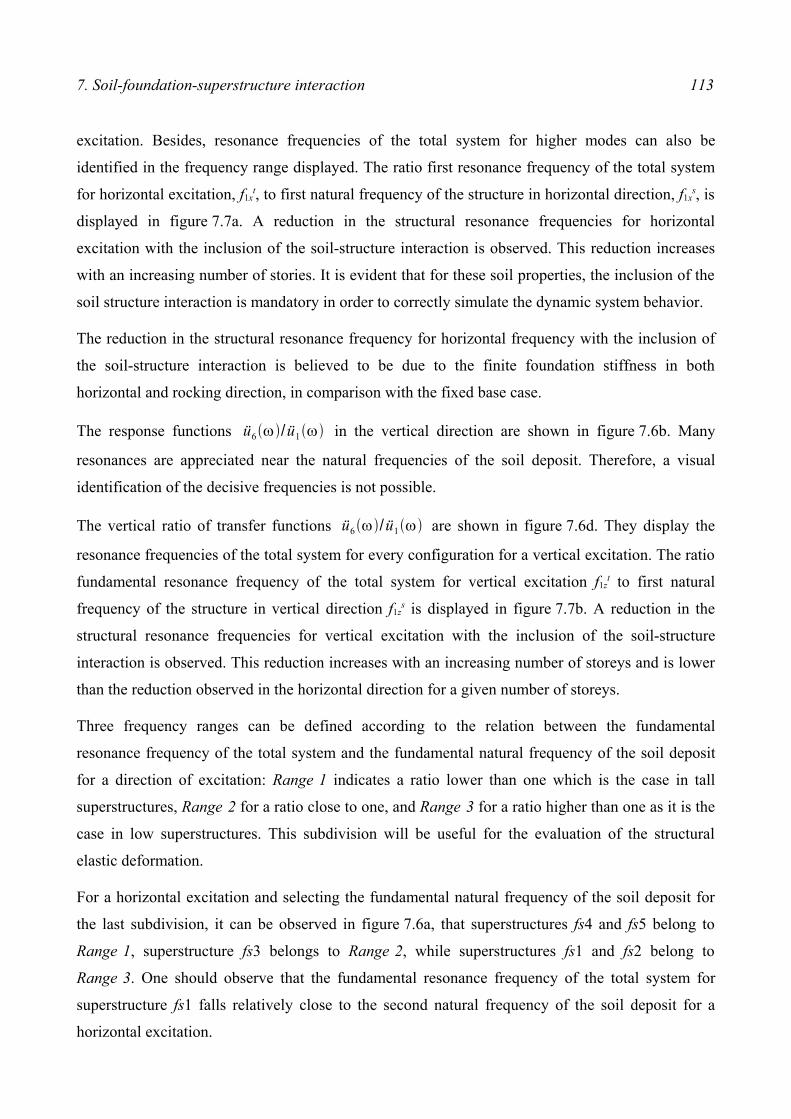
7. Soil-foundation-superstructure interaction 113
excitation. Besides, resonance frequencies of the total system for higher modes can also be
identified in the frequency range displayed. The ratio first resonance frequency of the total system
for horizontal excitation, f1xt, to first natural frequency of the structure in horizontal direction, f1x
s, is
displayed in figure 7.7a. A reduction in the structural resonance frequencies for horizontal
excitation with the inclusion of the soil-structure interaction is observed. This reduction increases
with an increasing number of stories. It is evident that for these soil properties, the inclusion of the
soil structure interaction is mandatory in order to correctly simulate the dynamic system behavior.
The reduction in the structural resonance frequency for horizontal frequency with the inclusion of
the soil-structure interaction is believed to be due to the finite foundation stiffness in both
horizontal and rocking direction, in comparison with the fixed base case.
The response functions ü6ω/ü1ω in the vertical direction are shown in figure 7.6b. Many
resonances are appreciated near the natural frequencies of the soil deposit. Therefore, a visual
identification of the decisive frequencies is not possible.
The vertical ratio of transfer functions ü6ω/ü1ω are shown in figure 7.6d. They display the
resonance frequencies of the total system for every configuration for a vertical excitation. The ratio
fundamental resonance frequency of the total system for vertical excitation f1zt to first natural
frequency of the structure in vertical direction f1zs is displayed in figure 7.7b. A reduction in the
structural resonance frequencies for vertical excitation with the inclusion of the soil-structure
interaction is observed. This reduction increases with an increasing number of storeys and is lower
than the reduction observed in the horizontal direction for a given number of storeys.
Three frequency ranges can be defined according to the relation between the fundamental
resonance frequency of the total system and the fundamental natural frequency of the soil deposit
for a direction of excitation: Range 1 indicates a ratio lower than one which is the case in tall
superstructures, Range 2 for a ratio close to one, and Range 3 for a ratio higher than one as it is the
case in low superstructures. This subdivision will be useful for the evaluation of the structural
elastic deformation.
For a horizontal excitation and selecting the fundamental natural frequency of the soil deposit for
the last subdivision, it can be observed in figure 7.6a, that superstructures fs4 and fs5 belong to
Range 1, superstructure fs3 belongs to Range 2, while superstructures fs1 and fs2 belong to
Range 3. One should observe that the fundamental resonance frequency of the total system for
superstructure fs1 falls relatively close to the second natural frequency of the soil deposit for a
horizontal excitation.

114
0
10
20
30
40
50
60
0 5 10 15 20 25
|u6x
(ω)|
[
-]
frequency [Hz]
(a)
fs1fs2fs3fs4fs5
0
2
4
6
8
10
12
14
16
18
0 5 10 15 20 25|u
6z(ω
)|
[-
]
frequency [Hz]
(b)
fs1fs2fs3fs4fs5
0
2
4
6
8
10
12
14
16
18
0 5 10 15 20 25
|u6x
(ω)|
/ |u 1
x(ω
)|
[-]
frequency [Hz]
(c)
f1xd f2x
d f3xd
fs1fs2fs3fs4fs5
0
1
2
3
4
5
6
0 5 10 15 20 25
|u6z
(ω)|
/ |u 1
z(ω
)|
[-]
frequency [Hz]
(d)
f1zd f2z
d
fs1fs2fs3fs4fs5
Figure 7.6 Response functions for flexible superstructures on rigid massless surfacefoundations on a layer over rigid base under harmonic base excitation: a)Response function ü6 x ω due to a vertical propagating SV-wave; b)Response function ü6 z ω due to a vertical propagating P-wave; c) ratio oftransfer functions ü6 x ω/ü1 x ω due to a vertical propagating SV-wave; b)ratio of transfer functions ü6 z ω/ü1 z ω due to a vertical propagating P-wave.
For a vertical excitation, the fundamental resonance frequencies of the total system of the
investigated cases locate beyond the first natural frequencies of the soil deposit as it is displayed in
figure 7.6b. Therefore, all investigated cases fall in Range 3.

7. Soil-foundation-superstructure interaction 115
0
0.2
0.4
0.6
0.8
1
1 2 3 4 5
f 1xt /
f 1xs
[-
]
number of stories [-]
(a)
0
0.2
0.4
0.6
0.8
1
1 2 3 4 5f 1
zt / f 1
zs
[-]
number of stories [-]
(b)
Figure 7.7 Ratio first resonance frequency of the total system to first natural frequency ofthe structure for flexible superstructures on rigid massless surface foundationson a layer over rigid base under harmonic base excitation: a) verticalpropagating SV-wave; b) vertical propagating P-wave.
There are different ways to evaluate the structural safety. The absolute accelerations at every level
and especially at the highest level can be indicative of the acceleration input for secondary
structures or equipment located in the structure. The absolute displacements especially at the
highest level may show the possible collision with neighbor structures. The relative displacements
in the different structural members are directly related to the internal forces and stresses in that
member. Therefore, these last parameters are selected here to evaluate the dynamic structural
behavior.
The superstructure relative displacements are the difference between the displacement amplitudes
on the structure top and the displacement amplitudes on the foundation top. In frequency domain,
according to the addition property of the Fourier Transformation (Waller & Schmidt 1989), the
relative displacement amplitudes will be computed as the difference of the steady state complex
absolute displacement amplitudes of the corresponding magnitudes at the structure top minus those
at the foundation top.
The horizontal superstructure relative displacements due to a horizontal excitation are shown in
figures 7.8a. Relatively high values are observed on the superstructure relative displacement
amplitudes for resonance. Systems located in Range 3 (fs1 and fs2) display almost zero
superstructure relative displacement amplitudes. Systems located in Range 2 (fs3) are expected to

116
experience high
0.00
0.10
0.20
0.30
0.40
0.50
0.60
0.70
0.80
0.90
1.00
0 5 10 15 20 25
|u6x
(ω)
- u 5
x(ω
)|
[m
]
frequency [Hz]
(a)
f1xd
fs1fs2fs3fs4fs5
0.0000
0.0005
0.0010
0.0015
0.0020
0.0025
0.0030
0 5 10 15 20 25
|u6z
(ω)
- u 5
z(ω
)|
[m
]
frequency [Hz]
(b)
f1zd
fs1fs2fs3fs4fs5
Figure 7.8 Superstructure relative displacements for flexible superstructures on rigidmassless surface foundations on a layer over rigid base under harmonic baseexcitation: a) horizontal amplitudes due to a vertical propagating SV-wave; b)vertical amplitudes due to a vertical propagating P-wave.
structural relative displacement amplitudes. For systems located in Range 1 (fs4 and fs5) very high
superstructure relative displacement amplitudes are observed because of the low frequency range
and the relationship between displacements u j ω and accelerations ü j ω stated in equation (3-
26) and rewritten:
ü j ω =ω 2 u j ω .
The vertical superstructure relative displacements are shown in figures 7.8b. The highest
superstructure relative displacements occur for superstructure fs5, whose resonance frequency of
the total system falls closest to the the first natural frequency of the soil deposit among all cases
analysed.
For very low frequencies, numerical irregularities are observed in the relative displacements in both
horizontal and vertical directions, due to the inconsistency of pure harmonic excitation for almost
static excitation. Similar observations have been reported by Hudson (1956, 1962) regarding the
difference between the spectral relative velocity and the so-called pseudo-velocity spectral
response of a response spectra.

7. Soil-foundation-superstructure interaction 117
7.2.2 Influence of the foundation
The frame structure with two stories fs2 displays a fundamental resonance frequency of the total
system in the horizontal direction of about 3.0 Hz and in the vertical direction of about 17.5 Hz.
The mechanical parameters are modified as listed in table 7.4 in order to get resonance frequencies
of the total system close to the fundamental horizontal and vertical natural frequencies of the soil
deposit for horizontal and vertical excitations (f1xd=2.03 Hz, f1z
d=4.98 Hz). For the new mechanical
parameters, the structure on a rigid massless surface foundation displays a fundamental resonance
frequency of the total system in the horizontal direction of about 2.4 Hz and in the vertical direction
of about 5.3 Hz. This structure belongs to Range 2 and very high resonance amplitudes are
therefore expected. This building is analysed with the different foundation systems listed in
table 7.5.
Table 7.4 Modified flexible superstructure fs2. Geometric and mechanic parameters.
System number ofstoreys
B h columnsEA
columnsEI
slabmass
slabsthickness
f1xs f1z
s
[m] [m] [MN] [MN m 2] [kg] [m] [Hz] [Hz]fs2 2 1.80 7.00 544.00 418.20 3240.00 0.30 5.02 21.54
Table 7.5 Foundation configurations considered.
System number of piles
L d α
[m] [m] [°]fc1 - - - -fc2 4 9.00 0.60 0.00fc3 4 9.00 0.60 31.00fc4 4 0.60 0.60 0.00
The analysed problem corresponds to the following configuration:
• Subsoil configuration: homogeneous layer over rigid base (layer over rigid base)
• Flexible superstructure modelled with a stick model
• Different foundation configurations:
a) Foundation configuration 1, fc1: rigid massless surface foundation
b) Foundation configuration 2, fc2: 2x2 vertical long pile group rigidly fixed to rigid

118
massless a surface foundation
c) Foundation configuration 3, fc3: 2x2 inclined pile group rigidly fixed to a rigid massless
surface foundation
d) Foundation configuration 4, fc4: 2x2 vertical short pile group rigidly fixed to a rigid
massless surface foundation
• Harmonic base excitation at the top of the rigid base:
a) Upward vertical propagating SV-wave
b) Upward vertical propagating P-wave
The horizontal and vertical ratio of transfer functions are shown in figure 7.9a and figure 7.9b.
It can be observed in figure 7.9a that the inclusion of piles in the foundation increases the
horizontal stiffness of the system and can shift the horizontal fundamental resonance frequency of
the total system considerably. Even the effect of short piles, which can be compared with a typical
embedded plate foundation, is remarkable.
0
5
10
15
20
25
0 2 4 6 8 10
|u6x
(ω)|
/ |u 1
x(ω
)|
[-]
frequency [Hz]
(a)
f1xd
fc1fc2fc3fc4
0
2
4
6
8
10
12
14
16
18
20
0 2 4 6 8 10
|u6z
(ω)|
/ |u 1
z(ω
)|
[-]
frequency [Hz]
(b)
f1zd
fc1fc2fc3fc4
Figure 7.9 Ratio of transfer functions ü6ω/ü1ω for modified superstructure fs2 ondifferent foundation configurations on a layer over rigid base under harmonicbase excitation: a) vertical propagating SV-wave; b) vertical propagating P-wave.
The vertical fundamental resonance frequencies of the total system for the four cases does not
differ considerably as can be observed in figure 7.9b.

7. Soil-foundation-superstructure interaction 119
The difference between the behaviors due to a horizontal excitation and due to a vertical excitation,
can be explained with the stiffness increment between a surface foundation and a deep foundation
(say vertical pile foundation) with the same plan area, as it was discussed in chapter 6.4.2.1.
Although the stiffness increments in the translational x- and z-directions are of the similar
magnitude, the increment in the rocking direction is about 10 times the increment in the
translational directions. That means, the rocking deformability is considerably reduced in a
structure with deep foundation, in comparison with the same structure but on a surface foundation.
The "horizontal superstructure relative displacement amplitudes" are exhibited in figures 7.10a.
The "vertical superstructure relative displacement amplitudes" are exhibited in figures 7.10b.
For an excitation defined in the horizontal direction, the maximal relative displacement of the
structure founded on vertical piles fc2 is about 9% of the maximal relative displacement of the
structure founded on a surface foundation fc1; the maximal relative displacement of the structure
founded on inclined piles fc3 is about 4% of the maximal relative displacement of the structure
founded on a surface foundation fc1; the maximal relative displacement of the structure founded on
vertical short piles fc4 is about 19% of the maximal relative displacement of the structure founded
on a surface foundation fc1. It is evident that the inclusion of piles produces a decisive amplitude
reduction in the harmonic relative accelerations and harmonic relative displacements in the
superstructure, because of the effective shift of the system to a frequency range with lower
acceleration amplitudes.
For an excitation defined in the vertical direction, the maximal relative displacement of the
structure founded on vertical piles fc2 is about 55% of the maximal relative displacement of the
structure founded on a surface foundation fc1; the maximal relative displacement of the structure
founded on inclined piles fc3 is about 68% of the maximal relative displacement of the structure
founded on a surface foundation fc1; the maximal relative displacement of the structure founded on
vertical short piles fc4 is about 91% of the maximal relative displacement of the structure founded
on a surface foundation fc1. A reduction in the vertical maximal relative displacement amplitude of
the structure is observed for the systems on deep foundations (fc2, fc3, and fc4) in comparison with
the vertical maximal relative displacement amplitudes of the structure on a surface foundation
(fc1).
The effectiveness of the deep foundations for the vibration reduction of the investigated cases is
higher for horizontal excitations, than for vertical excitations, because of the different influence of
the deep foundations in the resonance frequencies of the total system for horizontal excitations in
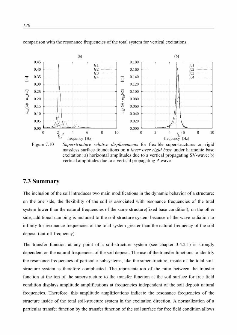
120
comparison with the resonance frequencies of the total system for vertical excitations.
0.00
0.05
0.10
0.15
0.20
0.25
0.30
0.35
0.40
0.45
0 2 4 6 8 10
|u6x
(ω)
- u 5
x(ω
)|
[m
]
frequency [Hz]
(a)
f1xd
fc1fc2fc3fc4
0.000
0.020
0.040
0.060
0.080
0.100
0.120
0.140
0.160
0.180
0 2 4 6 8 10
|u6z
(ω)
- u 5
z(ω
)|
[m
]
frequency [Hz]
(b)
f1zd
fc1fc2fc3fc4
Figure 7.10 Superstructure relative displacements for flexible superstructures on rigidmassless surface foundations on a layer over rigid base under harmonic baseexcitation: a) horizontal amplitudes due to a vertical propagating SV-wave; b)vertical amplitudes due to a vertical propagating P-wave.
7.3 Summary
The inclusion of the soil introduces two main modifications in the dynamic behavior of a structure:
on the one side, the flexibility of the soil is associated with resonance frequencies of the total
system lower than the natural frequencies of the same structure(fixed base condition); on the other
side, additional damping is included to the soil-structure system because of the wave radiation to
infinity for resonance frequencies of the total system greater than the natural frequency of the soil
deposit (cut-off frequency).
The transfer function at any point of a soil-structure system (see chapter 3.4.2.1) is strongly
dependent on the natural frequencies of the soil deposit. The use of the transfer functions to identify
the resonance frequencies of particular subsystems, like the superstructure, inside of the total soil-
structure system is therefore complicated. The representation of the ratio between the transfer
function at the top of the superstructure to the transfer function at the soil surface for free field
condition displays amplitude amplifications at frequencies independent of the soil deposit natural
frequencies. Therefore, this amplitude amplifications indicate the resonance frequencies of the
structure inside of the total soil-structure system in the excitation direction. A normalization of a
particular transfer function by the transfer function of the soil surface for free field condition allows

7. Soil-foundation-superstructure interaction 121
then the identification of the resonance frequencies of this particular subsystem inside of the total
system in the excitation direction.
The harmonic behavior of different frame structures on surface foundations with same geometrical
and mechanical configuration was investigated. This analysis indicates that the reduction of the
resonance frequencies of the total system due to soil-structure interaction under horizontal
excitation is higher for an increasing number of storeys. Similar behavior was observed for vertical
excitations.
The contribution of the geometrical attenuation of the soil in the acceleration amplitude reduction
in the structure is found to be higher for structures with relatively high resonance frequencies for
the total system. This is the case of relatively light constructions and with low height.
An evaluation of the behavior of a structure on a soil layer due to a base excitation at the layer base
is made through a comparison between two frequency sets: the resonance frequencies of the total
system and the natural frequencies of the soil deposit in the excitation direction. If any frequency of
the former frequency set approaches any frequency of the latter set, very high acceleration and
displacement amplitudes are observed in the structure. The highest interaction occurs when the
fundamental natural frequency of the soil deposit approaches the fundamental resonance frequency
of the total system.
The harmonic behavior of a superstructure on a surface foundation on a soil layer overlaying a rigid
base due to a base excitation was analysed. The fundamental resonance frequency of the total
system approaches the fundamental natural frequency of the soil deposit for horizontal excitation.
Similar condition is also satisfied for vertical excitation. This behavior was compared with that of
the same superstructure but with different embedded foundation configurations: vertical pile group,
inclined pile group and vertical short pile group.
It was observed that the fundamental resonance frequency of the total system for the structure on
vertical pile group for horizontal excitation increased 87% in comparison with the fundamental
resonance frequency of the total system for the structure on a surface foundation for horizontal
excitation. The fundamental resonance frequency of the total system for the structure on an inclined
pile group for horizontal excitation increased 96% in comparison with the fundamental resonance
frequency of the total system of the structure on a surface foundation for horizontal excitation. The
fundamental resonance frequency of the total system for the structure on a vertical short pile group
for horizontal excitation increased 29% in comparison with the fundamental resonance frequency
of the total system of the structure on a surface foundation for horizontal excitation.

122
The vertical pile group and the inclined pile group were effective to reduce the horizontal
acceleration amplitudes and the horizontal displacement amplitudes of the superstructure subjected
to a horizontal excitation in comparison with the horizontal acceleration amplitudes and the
horizontal displacement amplitudes of the superstructure founded on a surface foundation subjected
to a horizontal excitation.
It was observed that the fundamental resonance frequency of the total system for the structure on
vertical pile group for vertical excitation increased 2.9% in comparison with the fundamental
resonance frequency of the total system for the structure on a surface foundation for vertical
excitation. The fundamental resonance frequency of the total system for the structure on an inclined
pile group for vertical excitation increased 3.0% in comparison with the fundamental resonance
frequency of the total system of the structure on a surface foundation for vertical excitation. The
fundamental resonance frequency of the total system for the structure on a vertical short pile group
for vertical excitation increased 0.9% in comparison with the fundamental resonance frequency of
the total system of the structure on a surface foundation for vertical excitation.
For the investigated deep foundations: a vertical pile group, an inclined pile group and a vertical
short pile group, less effectiveness was detected to reduce vibration amplitudes in the
superstructure due to a vertical excitation in comparison with the reduction of the vibration
amplitudes in the superstructure for the same foundation cases but subjected to horizontal
excitation.

8. Reduction of seismically induced vibration in structures using deep foundations 123
8. Reduction of seismically induced vibration in structures
using deep foundations
Strategies to reduce seismically induced vibrations in structures are proposed, for both horizontal
and vertical excitations. The effectiveness of the strategies for the excitation direction is
commented. The proposed procedure is illustrated with an example.
8.1 Design strategy
8.1.1 Reduction of vertical vibrations induced by vertical seismic excitation
It is assumed that the soil conditions, the superstructure and the seismic excitations are given. The
objective is to select a foundation system able to reduce the vertical seismic induced vibrations in
the superstructure.
In case of a vertical excitation, advantage can be taken usually only of the soil-foundation
interaction. A "dynamic stiff foundation" (deep foundations, for example) experiences lower
vertical acceleration amplitudes in the near field than the vertical acceleration amplitudes in near
field experienced by a surface foundation. A reduction in the near field amplitudes is associated
with a reduction in the total vertical acceleration amplitudes in the structure, as well as with a
reduction in the vertical acceleration amplitudes of the input motion for secondary structures.
However, the relative vertical acceleration amplitudes in the superstructure are not expected to be
modified by the selection of the foundation.
8.1.2 Reduction of horizontal vibrations induced by horizontal seismic excitation
It is assumed that the soil conditions, the superstructure and the seismic excitations are given. The
objective is to select a foundation system able to reduce the horizontal seismic induced vibrations
in the superstructure.
The soil deposit consists of a stratified medium and is characterized by its natural frequencies. It
will be identified by the first natural frequency of the soil deposit in the horizontal direction f1xd .
The structure is characterized by its natural frequencies without consideration of the soil. It will be
identified by the fundamental natural frequency of the structure for a horizontal excitation f1xs.
124
The seismic excitation consists of a site specific design spectra (Clough & Penzien 1993) and is
identified by the frequency range, [f]xse, containing the decisive horizontal acceleration amplitudes.
One should realize that, due to the characteristics of the excitation, f1xd is always included in [f]x
se.
The proposed procedure can be summarized as follows:
(1)Select an initial foundation configuration. It is recommended to select a shallow embedded
foundation, due to its low costs.
(2)Compute the ratio between the transfer function at the top of the superstructure and the transfer
function at the soil surface for free field ü6ω/ü1ω of the soil-foundation-superstructure
model, and determine the fundamental resonance frequency of the total system for a horizontal
excitation f1xt. Due to the soil-structure interaction, it is known that: f1x
t < f1xs.
(3)Identify the applicability of the current strategy from the relationship between the characteristic
values of the system: f1xd, [f]x
se, f1xs, and f1x
t. Following possibilities exist:
(a) f1xt > [f]x
se. In this case, no measure is required. This is usually the case for relatively
very low and very light structures.
(b) f1xt is included in [f]x
se and f1xs > [f]x
se. A measure is required and the current strategy
applies. This is the case for relatively low structures.
(c) f1xt is included in [f]x
se and f1xs is also included in [f]x
se. A measure is required, but the
current strategy does not apply. A more flexible soil-structure connection like the usual
base isolation devices can be useful. This is the case for relatively middle tall structures.
(d) f1xt < [f]x
se and f1xs is included in [f]x
se. No measure is required. This is the case for
relatively tall structures.
(e) f1xt < [f]x
se and f1xs < [f]x
se. No measure is required. This is the case for relatively very tall
structures.
(4) Select a dynamically stiffer foundation, compute f1xt as it was explained in (2) and compare it
with [f]xse.
(5) If f1xt > [f]x
se the goal is reached and the procedure is finished. If f1xt is included in [f]x
se, repeat
step (4).
Special care should be taken to avoid the coincidence of f1xt with higher resonance frequencies of
the site for a horizontal excitation.

8. Reduction of seismically induced vibration in structures using deep foundations 125
In the following, the application of the proposed procedure is illustrated with an example.
8.2 Example description
The selected superstructure consists of a three-storey frame building with the geometrical
configuration displayed in figure 8.1a and the mechanical and geometrical parameters listed in
table 8.1. The subsoil conditions are displayed in figure 8.1b with mechanical and geometrical
parameters listed in table 8.2. The seismic environment consists of upward vertically propagating
body waves travelling from the rigid base rock to the free field surface as it is schematically
represented in figure 8.1b. The synthetic acceleration history generated in chapter 5.2 and displayed
in figure 8.2 is used as input rock motion.
h
h
h
2B
2Bt
t
t
EAEI
(a)
y
z
x
rigid base
body waves
x
z
free surface
soil layer8 8H
(b)
Figure 8.1 Case example analysed: a) superstructure configuration; b) subsoilconditions and seismic environment.
8.2.1 Identification of the system
8.2.1.1. Identification of the site
Assuming a harmonic base motion at the rock base, the transfer functions at the free surface for
horizontal and vertical excitations computed in chapter 5.1 are redisplayed in figures 8.3a and 8.3b.
Using equation (2-7), the first three natural frequencies of the soil deposit in horizontal direction
are computed (see section 5.1.1): f1xd=2.03 Hz, f2x
d=6.20 Hz and f3xd=10.1 Hz. For a vertical
excitation, the first and second natural frequencies of the soil deposit are (see section 5.1.2):
f1zd=4.98 Hz, and f2z
d=14.95 Hz.

126
8.2.1.2. Identification of the excitation
The horizontal seismic excitation consists of the simulated acceleration history (figure 8.2)
prescribed at the rigid base rock (figure 8.1) as vertically propagating SV-waves. As stated in
equation (3-10), the seismic excitation are equivalent seismic loads depending on the free field
displacements at the interaction nodes. Therefore, the acceleration history at the free surface
computed from free field is replaced by an "equivalent" excitation of the structure. The Fourier
amplitude spectrum and the acceleration time history of the horizontal free field acceleration are
redisplayed in figure 8.4. The frequency range, [f]xse, containing the decisive horizontal acceleration
amplitudes is selected from 1.82 to 2.35 Hz.
Table 8.1 Mechanical and geometricalparameters of superstructure.
Columns Slabsh EA EI 2B t dead+
live load[m] [MN] [MN m2] [m] [m] [N/m2]3,5 3060 1480 8,13 0,3 10000
Table 8.2 Mechanical parameters of soil layer overlaying a rigid base.
System E ν ρ β H
[MN/m2] [-] [kg/m3] [-] [m]Soil 42.0 0,40 1800,0 0,05 11,25
0.0
0.5
1.0
1.5
2.0
2.5
3.0
3.5
4.0
4.5
0 5 10 15 20 25
|u (ω
)|
[m/s
2 /Hz]
frequency [Hz]
(a)
-2.0
-1.0
0.0
1.0
2.0
0 10 20 30 40 50 60 70 80
u (t
) [
m/s
2 ]
time [s]
(b)
1.00
Figure 8.2 Simulated acceleration history: a) Fourier amplitude spectrum; b) time history.

8. Reduction of seismically induced vibration in structures using deep foundations 127
0
2
4
6
8
10
12
14
0 5 10 15 20 25
|u1x
(ω)|
[
m/s
2 /Hz]
frequency [Hz]
(a)
f1xd=2.03
0
2
4
6
8
10
12
14
0 5 10 15 20 25|u
1z(ω
)|
[m/s
2 /Hz]
frequency [Hz]
(b)
f1zd=4.98
Figure 8.3 Free field surface transfer function due to a harmonic base excitation:a) vertically propagating SV-wave; b) vertically propagating P-wave
In a similar way, the "equivalent" vertical seismic excitation is the free field surface acceleration
history computed in chapter 5.3 from the upward vertically propagating P-wave input rock motion.
The Fourier amplitude spectrum and the acceleration time history of the vertical free field
acceleration are redisplayed in figure 8.5. The frequency range, [f]zse, containing the decisive
vertical acceleration amplitudes is selected from 4.29 to 5.68 Hz.
8.2.1.3. Identification of the structure
The dynamic identification of the structure is performed through a modal analysis. For this
purpose, a discretization of the structure is required. The distributed dead and live load at the slabs
is considered through an equivalent mass density. As a first step, the fundamental frequency of the
slabs is computed through equation (7-1) (see page 109) in order to evaluate its vertical flexibility:
f 1slab=5.7
2 π 3.4 x10100.32
3333.337.5410.252=15.95 Hz
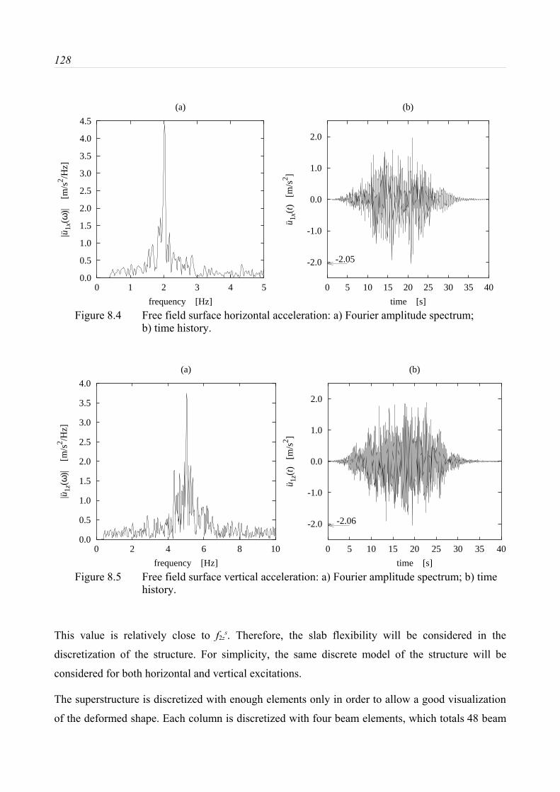
128
0.0
0.5
1.0
1.5
2.0
2.5
3.0
3.5
4.0
4.5
0 1 2 3 4 5
|u1x
(ω)|
[m
/s2 /H
z]
frequency [Hz]
(a)
-2.0
-1.0
0.0
1.0
2.0
0 5 10 15 20 25 30 35 40u 1
x(t)
[m
/s2 ]
time [s]
(b)
-2.05
Figure 8.4 Free field surface horizontal acceleration: a) Fourier amplitude spectrum;b) time history.
0.0
0.5
1.0
1.5
2.0
2.5
3.0
3.5
4.0
0 2 4 6 8 10
|u1z
(ω)|
[m
/s2 /H
z]
frequency [Hz]
(a)
-2.0
-1.0
0.0
1.0
2.0
0 5 10 15 20 25 30 35 40
u 1z(
t)
[m/s
2 ]
time [s]
(b)
-2.06
Figure 8.5 Free field surface vertical acceleration: a) Fourier amplitude spectrum; b) timehistory.
This value is relatively close to f2zs. Therefore, the slab flexibility will be considered in the
discretization of the structure. For simplicity, the same discrete model of the structure will be
considered for both horizontal and vertical excitations.
The superstructure is discretized with enough elements only in order to allow a good visualization
of the deformed shape. Each column is discretized with four beam elements, which totals 48 beam

8. Reduction of seismically induced vibration in structures using deep foundations 129
elements in the superstructure. Each plate is discretized with 64 plate elements, which results in a
total of 192 plate elements in the superstructure.
Considering a fixed base condition, a modal analysis is performed for the superstructure with the
program ANSYS (1996). The modal frequencies are listed in table 8.3 and the modal shapes are
displayed in the annex C. The first and second natural frequencies of the structure for horizontal
excitation are f1xs=2.92 Hz and f2x
s=15.48 Hz. It can be observed that f1xs is higher than [f]x
se as it is
required in order to apply the proposed methodology. For vertical excitation, the first, second and
third natural frequencies of the structure are f1zs=7.70 Hz, f2z
s=8.33 Hz and f3zs=8.39 Hz, which show
a very close spacing among them.
Table 8.3 Superstructure modal frequencies considering a fixed base condition.
n fn modal form description
[Hz]1 2,92 Horizontal: y-z2 2,92 Horizontal: x-z3 5,03 Torsion4 7,69 Vertical5 8,33 Vertical6 8,39 Vertical7 15,02 Rocking: xx8 15,02 Rocking: yy9 15,48 Horizontal: y-z
10 15,48 Horizontal: x-z
8.2.2 Analysed cases
The considered superstructure is analysed with four different foundation configurations as it is
displayed in figure 8.6. First, a relatively shallow embedded plate foundation is selected. Then,
three different deep foundations are considered. The following foundation systems are considered
for the same superstructure:

130
Figure 8.6 Analysed cases: a) Case 1; b) Case 2; c) Case 3; d) Case 4.
Case 1
:
A shallow embedded slab foundation, with top surface coinciding with the ground surface
level.Case 2
:
4x4 vertical pile group rigidly connected to an embedded pile cap.
Case 3
:
4x4 inclined and vertical pile group rigidly connected to an embedded pile cap.
Case 4
:
A soil improvement block underlaying a shallow embedded slab foundation. Equivalentmechanical parameters from Case 2 are selected (see chapter 6.5.1). Case 4a refers to thefoundation mechanical parameters for the case of a vertical excitation and Case 4bcorresponds to the foundation mechanical parameters for the case of a horizontal excitation.
The mechanical and geometrical parameters are listed in table 8.4.
Table 8.4 Mechanical and geometrical parameters of different foundation casesconsidered.
System E ν ρ β B t L d s n α
[MN/m2] [-] [kg/m3] [-] [m] [m] [m] [m] [m] [-] [°]Case 1 42000 0,25 2500,0 0,02 8,13 0,6 - - - - -Case 2 42000 0,25 2500,0 0,02 8,13 0,6 9,00 0,60 2,5 16 0,00
Case 3 42000 0,25 2500,0 0,02 8,13 0,6 9,00 0,60(on top)
2.5 16 53,10Case 4a 2950 0,45 1860,0 0,02 8,13 0,6 9,00 - - - -Case 4b 3940 0,45 1860,0 0,02 8,13 0,6 9,00 - - - -
The discretization of the foundation systems is done according to the recommendations established
in chapter 4.2.2.4. The slab foundation as well as the pile cap is modeled with 144 volume
elements.
t
(a)
L
t
(b) (c) (d)
L L
t t
�
ds

8. Reduction of seismically induced vibration in structures using deep foundations 131
Figure 8.7 Discretization meshes utilized. Top left: Case 1; top right: Case 2; bottom left:Case 3; bottom right: Case 4.
The piles are modeled with 16x12=192 beam elements. The soil improvement block is modeled
with 16x12=192 volume elements. The discretization meshes utilized are displayed in figure 8.7.
The ground surface and the rigid rock base levels are also displayed for visualization purposes. In
order to transmit the moments from beam elements representing columns and piles to the volume
elements representing the slab foundation, plate elements with very high stiffness parameters are
connected over the volume elements, as it is displayed in figure 8.8.

132
beam elements:column
beam elements:pile
plateelement
volumeelement:pile cap/slab foundation
Figure 8.8 Intersection volumen-, plate- and beam- elements.
8.2.3 Results
8.2.3.1 Excitation in the horizontal direction
The ratio between the transfer function at the top of the structure and the transfer function at the
soil surface for free field for horizontal excitation, ü6ω/ü1ω , is displayed in figure 8.9, where
for convenience only a selected frequency range is shown.
It can be observed that for Case 1, f1xt =2.3 Hz. That means f1x
t is included in [f]xse and f1x
s > [f]xse.
The proposed strategy is therefore applicable. Regarding the deep foundation systems considered,
following ratios between the fundamental resonance frequency of the total system for a deep
foundation and the fundamental resonance frequency of the total system for a shallow foundation
are observed:
• f1xt Case 2 / f1x
t Case 1 = 1.16;
• f1xt Case 3 / f1x
t Case 1 = 1.20 and
• f1xt Case 4 / f1x
t Case 1 = 1.20.

8. Reduction of seismically induced vibration in structures using deep foundations 133
0
2
4
6
8
10
12
14
0 1 2 3 4 5
|u6x
(ω)|
/ |u 1
x(ω
)|
[-]
frequency [Hz]
f1xd f1x
s
Case 1Case 2Case 3Case 4
Figure 8.9 Ratio between the transfer function at the top of the superstructure andthe transfer function at the soil surface for free field, ü6ω/ü1ω , forhorizontal excitation.
The harmonic deformation states for an excitation frequency equal to f1xd are exhibited in
figure 8.10. For Case 1, an evident coupling between translational x- and rotational y-deformations
can be observed at the foundation level; high elastic deformations are observed in the
superstructure. For Case 2, almost no rocking is observed at the foundation; the elastic
superstructure deformations are considerable lower than for Case 1. For Case 3, almost no rocking
is observed at the foundation; considerably lower amplitudes are observed. For Case 4, little
rocking is present and similar elastic superstructure deformations are observed to those from
Case 2.
The time histories and the Fourier amplitude spectra of the horizontal accelerations at the top of the
foundation are displayed in figure 8.11. The acceleration time histories are commented first. The
maximum amplitude obtained for Case 1 represents 106% of the maximum amplitude obtained at
the ground surface for free field condition. The maximum amplitude obtained for Case 2 represents
83% of the maximum amplitude obtained for Case 1. The maximum amplitude obtained for Case 3
represents 58% of the maximum amplitude obtained for Case 1. The maximum amplitude obtained
for Case 4 represents 52% of the maximum amplitude obtained for Case 1. The Fourier amplitude
spectra show similar behavior in the ratio of maximum amplitudes of the 4 cases investigated.
Lower contribution of the higher vibration modes is also observed.
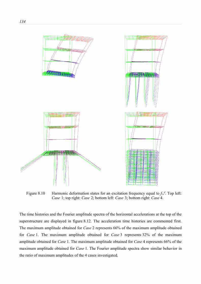
134
Figure 8.10 Harmonic deformation states for an excitation frequency equal to f1xd. Top left:
Case 1; top right: Case 2; bottom left: Case 3; bottom right: Case 4.
The time histories and the Fourier amplitude spectra of the horizontal accelerations at the top of the
superstructure are displayed in figure 8.12. The acceleration time histories are commented first.
The maximum amplitude obtained for Case 2 represents 66% of the maximum amplitude obtained
for Case 1. The maximum amplitude obtained for Case 3 represents 32% of the maximum
amplitude obtained for Case 1. The maximum amplitude obtained for Case 4 represents 66% of the
maximum amplitude obtained for Case 1. The Fourier amplitude spectra show similar behavior in
the ratio of maximum amplitudes of the 4 cases investigated.

8. Reduction of seismically induced vibration in structures using deep foundations 135
-2.0
-1.0
0.0
1.0
2.0
0 5 10 15 20 25 30 35 40
u 5x(
t)
[m/s
2 ]
time [s]
(a)
2.18
-2.0
-1.0
0.0
1.0
2.0
0 5 10 15 20 25 30 35 40
u 5x(
t)
[m/s
2 ]
time [s]
(b)
1.81
-2.0
-1.0
0.0
1.0
2.0
0 5 10 15 20 25 30 35 40
u 5x(
t)
[m/s
2 ]
time [s]
(c)
-1.26
-2.0
-1.0
0.0
1.0
2.0
0 5 10 15 20 25 30 35 40
u 5x(
t)
[m/s
2 ]
time [s]
(d)
1.14
0.0
1.0
2.0
3.0
4.0
5.0
6.0
0 5 10 15 20 25
|u5x
(ω)|
[m
/s2 /H
z]
frequency [Hz]
(e)
f1xd
0.0
1.0
2.0
3.0
4.0
5.0
6.0
0 5 10 15 20 25
|u5x
(ω)|
[m
/s2 /H
z]
frequency [Hz]
(f)
f1xd
0.0
1.0
2.0
3.0
4.0
5.0
6.0
0 5 10 15 20 25
|u5x
(ω)|
[m
/s2 /H
z]
frequency [Hz]
(g)
f1xd
0.0
1.0
2.0
3.0
4.0
5.0
6.0
0 5 10 15 20 25
|u5x
(ω)|
[m
/s2 /H
z]
frequency [Hz]
(h)
f1xd
Figure 8.11 Horizontal accelerations at the top of the foundation due to a horizontalexcitation. Acceleration time histories: a) Case 1; b) Case 2; c) Case 3; d) Case4. Fourier amplitude spectra: e) Case 1; f) Case 2; g) Case 3; h) Case 4.

136
-6.0
-4.0
-2.0
0.0
2.0
4.0
6.0
0 5 10 15 20 25 30 35 40
u 6x(
t)
[m/s
2 ]
time [s]
(a)
-5.99 -6.0
-4.0
-2.0
0.0
2.0
4.0
6.0
0 5 10 15 20 25 30 35 40
u 6x(
t)
[m/s
2 ]
time [s]
(b)
3.94
-6.0
-4.0
-2.0
0.0
2.0
4.0
6.0
0 5 10 15 20 25 30 35 40
u 6x(
t)
[m/s
2 ]
time [s]
(c)
-1.91
-6.0
-4.0
-2.0
0.0
2.0
4.0
6.0
0 5 10 15 20 25 30 35 40
u 6x(
t)
[m/s
2 ]
time [s]
(d)
-3.97
0.0
5.0
10.0
15.0
20.0
0 5 10 15 20 25
|u6x
(ω)|
[m
/s2 /H
z]
frequency [Hz]
(e)
f1xd
0.0
5.0
10.0
15.0
20.0
0 5 10 15 20 25
|u6x
(ω)|
[m
/s2 /H
z]
frequency [Hz]
(f)
f1xd
0.0
5.0
10.0
15.0
20.0
0 5 10 15 20 25
|u6x
(ω)|
[m
/s2 /H
z]
frequency [Hz]
(g)
f1xd
0.0
5.0
10.0
15.0
20.0
0 5 10 15 20 25
|u6x
(ω)|
[m
/s2 /H
z]
frequency [Hz]
(h)
f1xd
Figure 8.12 Horizontal accelerations at the top of the superstructure due to a horizontalexcitation. Acceleration time histories: a) Case 1; b) Case 2; c) Case 3; d) Case4. Fourier amplitude spectra: e) Case 1; f) Case 2; g) Case 3; h) Case 4.

8. Reduction of seismically induced vibration in structures using deep foundations 137
-0.03
-0.02
-0.01
0.00
0.01
0.02
0.03
0 5 10 15 20 25 30 35 40
u 6x(
t) -
u5x
(t)
[m
]
time [s]
(a)
0.025
-0.03
-0.02
-0.01
0.00
0.01
0.02
0.03
0 5 10 15 20 25 30 35 40
u 6x(
t) -
u5x
(t)
[m
]
time [s]
(b)
-0.016
-0.03
-0.02
-0.01
0.00
0.01
0.02
0.03
0 5 10 15 20 25 30 35 40
u 6x(
t) -
u5x
(t)
[m
]
time [s]
(c)
-0.005
-0.03
-0.02
-0.01
0.00
0.01
0.02
0.03
0 5 10 15 20 25 30 35 40
u 6x(
t) -
u5x
(t)
[m
]
time [s]
(d)
0.015
0.00
0.02
0.04
0.06
0.08
0.10
0 5 10 15 20 25
|u6x
(ω)
- u 5
x(ω
)|
[m/H
z]
frequency [Hz]
(e)
f1xd
0.00
0.02
0.04
0.06
0.08
0.10
0 5 10 15 20 25
|u6x
(ω)
- u 5
x(ω
)|
[m/H
z]
frequency [Hz]
(f)
f1xd
0.00
0.02
0.04
0.06
0.08
0.10
0 5 10 15 20 25
|u6x
(ω)
- u 5
x(ω
)|
[m/H
z]
frequency [Hz]
(g)
f1xd
0.00
0.02
0.04
0.06
0.08
0.10
0 5 10 15 20 25
|u6x
(ω)
- u 5
x(ω
)|
[m/H
z]
frequency [Hz]
(h)
f1xd
Figure 8.13 Horizontal relative displacements in the superstructure due to a horizontalexcitation. Displacement time histories: a) Case 1; b) Case 2; c) Case 3;d) Case 4. Fourier amplitude spectra: e) Case 1; f) Case 2; g) Case 3; h) Case 4.

138
The time histories, u6x(t)-u5x(t), and the Fourier amplitude spectra, |u6x(ω)-u5x(ω)|, of the horizontal
relative displacements in the superstructure are displayed in figure 8.13. The displacement time
histories are commented first. The maximum amplitude obtained for Case 2 represents 63% of the
maximum amplitude obtained for Case 1. The maximum amplitude obtained for Case 3
represents 26% of the maximum amplitude obtained for Case 1.The maximum amplitude obtained
for Case 4 represents 63% of the maximum amplitude obtained for Case 1. The Fourier amplitude
spectra show similar behavior in the ratio of maximum amplitude of the 4 cases investigated.
8.2.3.2 Excitation in the vertical direction
The time histories, ü5z(t), and Fourier amplitude spectra, |ü5z(ω)|, of the vertical accelerations at the
top of the foundation are displayed in figure 8.14. The acceleration time histories are commented
first. The maximum amplitude obtained for Case 1 represents 94% of the maximum amplitude
obtained at the ground surface for free field condition. The maximum amplitude obtained for
Case 2 represents 72% of the maximum amplitude obtained for Case 1. The maximum amplitude
obtained for Case 3 represents 84% of the maximum amplitude obtained for Case 1. The maximum
amplitude obtained for Case 4 represents 64% of the maximum amplitude obtained for Case 1. The
Fourier amplitude spectra show similar behavior in the ratio of maximum amplitude of the four
cases investigated. Lower contribution of the higher vibration modes is also observed.
The time histories, ü6z(t), and Fourier amplitude spectra, |ü6z(ω)|, of the vertical accelerations at the
top of the superstructure are displayed in figure 8.15. The acceleration time histories are
commented first. The maximum amplitude obtained for Case 2 represents 74% of the maximum
amplitude obtained for Case 1. The maximum amplitude obtained for Case 3 represents 87% of the
maximum amplitude obtained for Case 1. The maximum amplitude obtained for Case 4 represents
63% of the maximum amplitude obtained for Case 1. Similar ratios are observed as those at the
foundation top.
The Fourier amplitude spectra show similar behavior in the ratio of maximum amplitude of the four
cases investigated.

8. Reduction of seismically induced vibration in structures using deep foundations 139
-2.0-1.5-1.0-0.50.00.51.01.52.0
0 5 10 15 20 25 30 35 40
u 5z(
t)
[m/s
2 ]
time [s]
(a)
1.94
-2.0-1.5-1.0-0.50.00.51.01.52.0
0 5 10 15 20 25 30 35 40
u 5z(
t)
[m/s
2 ]
time [s]
(b)
1.39
-2.0-1.5-1.0-0.50.00.51.01.52.0
0 5 10 15 20 25 30 35 40
u 5z(
t)
[m/s
2 ]
time [s]
(c)
1.64
-2.0-1.5-1.0-0.50.00.51.01.52.0
0 5 10 15 20 25 30 35 40
u 5z(
t)
[m/s
2 ]
time [s]
(d)
1.25
0.0
0.5
1.0
1.5
2.0
2.5
3.0
3.5
0 5 10 15 20 25
|u5z
(ω)|
[m
/s2 /H
z]
frequency [Hz]
(e)
f1zd
0.0
0.5
1.0
1.5
2.0
2.5
3.0
3.5
0 5 10 15 20 25
|u5z
(ω)|
[m
/s2 /H
z]
frequency [Hz]
(f)
f1zd
0.0
0.5
1.0
1.5
2.0
2.5
3.0
3.5
0 5 10 15 20 25
|u5z
(ω)|
[m
/s2 /H
z]
frequency [Hz]
(g)
f1zd
0.0
0.5
1.0
1.5
2.0
2.5
3.0
3.5
0 5 10 15 20 25
|u5z
(ω)|
[m
/s2 /H
z]
frequency [Hz]
(h)
f1zd
Figure 8.14 Vertical accelerations at the top of foundation due to a vertical excitation.Acceleration time histories: a) Case 1; b) Case 2; c) Case 3; d) Case 4. Fourieramplitude spectra: e) Case 1; f) Case 2; g) Case 3; h) Case 4.

140
-2.0
-1.0
0.0
1.0
2.0
0 5 10 15 20 25 30 35 40
u 6z(
t)
[m/s
2 ]
time [s]
(a)
-2.07 -2.0
-1.0
0.0
1.0
2.0
0 5 10 15 20 25 30 35 40
u 6z(
t)
[m/s
2 ]
time [s]
(b)
1.54
-2.0
-1.0
0.0
1.0
2.0
0 5 10 15 20 25 30 35 40
u 6z(
t)
[m/s
2 ]
time [s]
(c)
1.80
-2.0
-1.0
0.0
1.0
2.0
0 5 10 15 20 25 30 35 40
u 6z(
t)
[m/s
2 ]
time [s]
(d)
1.31
0.00.51.01.52.02.53.03.54.0
0 5 10 15 20 25
|u6z
(ω)|
[m
/s2 /H
z]
frequency [Hz]
(e)
f1zd
0.00.51.01.52.02.53.03.54.0
0 5 10 15 20 25
|u6z
(ω)|
[m
/s2 /H
z]
frequency [Hz]
(f)
f1zd
0.00.51.01.52.02.53.03.54.0
0 5 10 15 20 25
|u6z
(ω)|
[m
/s2 /H
z]
frequency [Hz]
(g)
f1zd
0.00.51.01.52.02.53.03.54.0
0 5 10 15 20 25
|u6z
(ω)|
[m
/s2 /H
z]
frequency [Hz]
(h)
f1zd
Figure 8.15 Vertical accelerations at the top of superstructure due to a vertical excitation.Acceleration time histories: a) Case 1; b) Case 2; c) Case 3; d) Case 4. Fourieramplitude spectra: e) Case 1; f) Case 2; g) Case 3; h) Case 4.

8. Reduction of seismically induced vibration in structures using deep foundations 141
-0.6
-0.4
-0.2
0.0
0.2
0.4
0.6
0 5 10 15 20 25 30 35 40
u 6z(
t) -
u5z
(t)
[m
m]
time [s]
(a)
0.46
-0.6
-0.4
-0.2
0.0
0.2
0.4
0.6
0 5 10 15 20 25 30 35 40
u 6z(
t) -
u5z
(t)
[m
m]
time [s]
(b)
0.43
-0.6
-0.4
-0.2
0.0
0.2
0.4
0.6
0 5 10 15 20 25 30 35 40
u 6z(
t) -
u5z
(t)
[m
m]
time [s]
(c)
0.43
-0.6
-0.4
-0.2
0.0
0.2
0.4
0.6
0 5 10 15 20 25 30 35 40
u 6z(
t) -
u5z
(t)
[m
m]
time [s]
(d)
-0.52
0.0000
0.0002
0.0004
0.0006
0.0008
0.0010
0 5 10 15 20 25
|u6z
(ω)
- u 5
z(ω
)|
[m/H
z]
frequency [Hz]
(e)
f1zd
0.0000
0.0002
0.0004
0.0006
0.0008
0.0010
0 5 10 15 20 25
|u6z
(ω)
- u 5
z(ω
)|
[m/H
z]
frequency [Hz]
(f)
f1zd
0.0000
0.0002
0.0004
0.0006
0.0008
0.0010
0 5 10 15 20 25
|u6z
(ω)
- u 5
z(ω
)|
[m/H
z]
frequency [Hz]
(g)
f1zd
0.0000
0.0002
0.0004
0.0006
0.0008
0.0010
0 5 10 15 20 25
|u6z
(ω)
- u 5
z(ω
)|
[m/H
z]
frequency [Hz]
(h)
f1zd
Figure 8.16 Vertical relative displacements due to a vertical excitation. Acceleration timehistories: a) Case 1; b) Case 2; c) Case 3; d) Case 4. Fourier amplitude spectra:e) Case 1; f) Case 2; g) Case 3; h) Case 4.

142
The time histories, u6z(t)-u5z(t), and Fourier amplitude spectra, |u6z(ω)-u5z(ω)|, of the vertical relative
displacements in the superstructure are displayed in figure 8.16. The time histories are commented
first. The maximum amplitude obtained for Case 2 represents 93% of the maximum amplitude
obtained for Case 1. The maximum amplitude obtained for Case 3 represents 93% of the maximum
amplitude obtained for Case 1. The maximum amplitude obtained for Case 4 represents 113% of
the maximum amplitude obtained for Case 1. The Fourier amplitude spectra show similar behavior
in the ratio of maximum amplitude of the 4 cases investigated.
8.3 Summary
The proposed strategy to reduce seismic induced vibrations in structures take advantage of the
ability of deep foundations: to reduce the vibration amplitudes in comparison with those
experienced at the ground surface for free field condition, namely seismic soil-foundation
interaction; and to shift the first resonance frequency of the total soil-structure system away from
the frequency range of high amplitudes, namely seismic inertial interaction. In case of horizontal
excitations, both the seismic soil-foundation interaction as well as the seismic inertial interaction
are found to be of importance. In case of vertical excitations, only the seismic soil-foundation
interaction is found to be considerable.
The strategy to reduce horizontal seismic induced vibration in structures is recommended to be
applied if certain conditions between the structural resonance frequencies and the frequency range
of decisive amplitudes of the excitation are fulfilled: on the one hand, the first resonance frequency
of the total system should be included in the frequency range of high amplitudes; on the other hand,
the first natural frequency of the structure should be higher than the frequency range of high
amplitudes. This is the case of relatively low structures.
The strategy to reduce vertical seismic induced vibration in structures can be applied without
restrictions.

9. Summary and recommendations for future research 143
9. Summary and recommendations for future research
To reduce horizontal and vertical seismic vibrations in structures a design strategy is proposed. To
simulate the dynamic behavior of soil-structure systems a numerical method is developed and
implemented. Special attention was given to investigate the influence of plate foundations, pile
foundations and soil improvement foundations (volumes of soil improvement underlaying surface
foundations) on the reduction of seismically induced vibrations in the structures.
The numerical method is formulated in the frequency domain, and the connection to the time
domain is given by Fourier transformation techniques. The structure is described with the Finite
Element Method and the unbounded soil with the Thin Layer Method, coupling the vibration of the
structure and the wave propagation in the soil. The response is supposed to vary linearly with the
load. Material energy dissipation is introduced in form of a linear hysteretic damping formulation.
Special consideration is given to a sufficient representation of pile foundations.
The proposal of a strategy to reduce seismic vibrations in structures is made after simulations of
seismic responses of different soil-structure systems with the implemented numerical method.
Special attention is dedicated to identify the separate influences on the structural response of three
aspects, namely the response of the soil without structure (free field response), the soil-foundation
interaction, and the inertial interaction.
The following behavior has been observed:
The free field response shows that a layered soil medium filters the frequencies and amplifies the
amplitudes of the incoming seismic waves. Significant differences for vertical and horizontal
excitations can be seen. This phenomena influences then the excitation to be transmitted to the
structure.
A reduction of the vibration amplitudes at the foundation can be reached with a foundation with
high moduli of the dynamic stiffness such as deep foundations (for example piles and soil
improvement foundations). Vertical piles are found to be suitable to reduce vibration amplitudes
due to vertical excitations, while inclined piles behaves better for horizontal excitations.
Similarities between the vertical seismic response of a close spaced vertical pile foundation and
that of an "equivalent" soil improvement foundation were found.
A procedure is established to identify the resonance frequency of a soil-structure system that
excites the individual natural vibration shapes of the structure for a determinate direction of
144
excitation (resonance frequencies of the total soil-structure system). The ratio of the first resonance
frequency of the total soil-structure system to the first natural frequency of the structure with a
fixed base condition characterizes the inertial interaction. If this ratio is much lower than one it
indicates high inertial interaction, while a ratio equal to one means no inertial interaction. In soft
soil conditions, structures on foundations with low moduli of dynamic stiffnesses, like surface
foundations, usually display a high inertial interaction while structures on deep foundations may
display almost no inertial interaction. Deep foundations show a lower inertial interaction in the
horizontal direction, than in the vertical direction, because of their ability to restrict the rocking
deformability. Coincidence between the first resonance frequency of the total system and the
frequency range of high amplitudes of the seismic excitation induces the most unfavourable
condition for the structural safety. However, the selection of a suitable foundation system can avoid
such unfavourable situation under horizontal excitations.
The reduction of the horizontal and vertical vibration amplitudes at the foundation, and the ability
of the foundation to shift the first coupled structural resonance frequency off from the frequency
range of high amplitudes of the horizontal excitation, are the main features of the strategy proposed
for reduction of seismically induced vibrations in structures.
The inclusion of the following features to the computer program developed in this dissertation is
desirable:
• A formulation to compute transfer functions for excitations consisting of incident body waves
from a damped elastic halfspace.
• An interpolation function of higher order than one to compute the displacements in the
subsystem soil deposit, which would increase the accuracy of the results, relax the discretization
criteria and reduce the computational time.
• A hybride time/frequency domain computation procedure that allows the simulation of nonlinear
behavior. Such an enhancement will make possible the validation of the computational model
and of the proposed strategy to reduce vibrations through comparison of numerical results with
experimental and field results where the response is highly influenced by specific forms of
nonlinear behavior.

References 145
References
[1] Abdalkareem, K. H. & Machida, A.: Effect of Vertical Motion of Earthquake on FailureMode and Ductility of RC Bridge Piers. 12th WCEE. Auckland, New Zealand: New ZealandSociety for Earthquake Engineering 2000.
[2] Abramowitz, M. & Stegun, I. A.: Handbook of Mathematical Functions. New York: DoverPublications, Inc. 1965.
[3] Anderson, J: A Dislocation Model for the Parkfield Earthquake. Bull. Seism. Soc. Am. 64(1974) 671 - 686.
[4] ANSYS, Theory Reference, Release 5.4, 1997.[5] Avilés, J. & Sánchéz-Sesma, F. J. : Foundation Isolation from Vibrations Using Piles as
Bariers. Journal of Engineering Mechanics, Vol. 114, No. 11 (1988) 1854 - 1869.[6] Bachmann, H. & Ammann, W.: Vibration in structures: Induced by Man and Machines.
Zurich, Switzerland: Structural Engineering Documents 3e, International Association forBridge and Structural Engineering 1987.
[7] Bathe, K. J.: Finite Element Procedures in Engineering Analysis. Englewood Cliffs, NewJersey: Prentice-Hall, Inc. 1982.
[8] Bathe, K. L., Wilson, E. L., & Peterson, F. E.: SAP IV - A Structural Analysis Programmfor Static and Dynamic Response of Linear Systems. Report No. EERC 73-11, EarthquakeEngineering Center, UCB 1974.
[9] Banerjee, P. K. & Mamoon, S. M.: A Fundamental Solution Due to a Periodic Point Forcein the Interior of an Elastic Half-Space. Earthquake Engineering and Structural Dynamics,Vol. 19 (1990) 91 - 105.
[10] Bode, C.: Numerische Verfahren zur Berechnung von Baugrund-Bauwerk-Interaktionen imZeitbereich mittels Greenscher Funktionen für den Halbraum. Dissertation, TechnischeUniversität Berlin 2000 (in German).
[11] Bolton, S. R., Ostby, P. A. & Russell, M. J.: USQ Implications of the SASSI Issue at theIdaho Nuclear Technology and Engineering Center (INTEC). Safety Analysis Workshop,June 13 - 18, Portland, Oregon, 1999.
[12] Brown, D. A., Morrison, C. & Reese, L. C.: Lateral Load Behavior of Pile Group in Sand.Journal of Geotechnical Engineering, 114, 11 (1988) 1261 - 1276.
[13] Buckle, I. G.: Passive Control of Structures for Seismic Loads. 12th World Conference ofEarthquake Engineering, Auckland, New Zealand 2000.
[14] Butterfield, R. & Banerjee, P. K.: The Elastic Analysis of Compressible Piles and PileGroups. Geotechnique, Vol.21 (1971) 43 - 60.
[15] Chen, J. Ch., Lysmer, J. & Seed, H. B.: Analysis of Local Variations in Free Field SeismicGround Motion. Report No. UCB/EERC-81/3. Berkeley: University of California, Berkeley1981.
[16] Chopra, A. K.: Dynamics of Structures. Second Edition. Upper Saddle River, New Jersey:Prentice-Hall 2001.
[17] Chouw, N.: Effect of Strong Vertical Ground Motion on Structural Responses. 11th
European Conference on Earthquake Engineering. Rotterdam: Balkema 1998.

146
[18] Chouw, N.: Berechnung von Tragwerkschwingungen unter Berücksichtigung desdynamischen Übertragungsverhaltens des Baugrunds. Technisch-wissenschaftlicheMitteilungen, Mitteilung Nr. 94-3. Bochum: Ruhr-Universität Bochum, Institut fürKonstruktiven Ingenieurbau 1994 (in German).
[19] Clough, R. W. & Penzien, J.: Dynamics of Structures. Second Edition. Singapore: McGraw-Hill Book Co. 1993.
[20] Cooley, J. W. & Tukey, J. W.: An Algorithm for the Machine Calculation of ComplexFourier Series. Mathematics of Computation, Vol. 19, No. 19 (1965) 297 - 301.
[21] Darbre, G. R.: Hybrid Frequency-Time-Domain Procedure for Nonlinear Dynamic Analysiswith Application to Nonlinear Soil-Structure Interaction. 9th World Conference onEarthquake Engineering, 9WCEE Organizing Committee, Japan Assn. For EarthquakeDisaster Prevention, Tokio, Vol.III (1989) 477 - 482.
[22] Dolling, H. J.: Die Abschirmung von Erschütterungen durch Bodenschlitze. Die Bautechnik,Nr.5 (1970) 151 - 158 (in German).
[23] Dolling, H. J.: Die Abschirmung von Drschütterungen durch Bodenschlitze. DieBautechnik, Nr.6 (1970) 193 - 204 (in German).
[24] Dobry, R. & Gazetas, G.: Horizontal Response of Piles in Layered Soils. Journal ofGeotechnical Engineering, Vol 110, No. 1 (1984) 20 - 40.
[25] Dobry, R. & Gazetas, G.: Simple Method for Dynamic Stiffness and Damping of FloatingPile Groups. Géotechnique 38, No. 4 (1988) 557 - 574.
[26] El-Naggar, M. H. & Novak, M.: Nonlinear Analysis for Dynamic Lateral Pile Response.Journal Soil Dynamics and Earthquake Engineering, Vol. 15, No. 4 (1996) 233 - 244.
[27] Elnashai, A. S., Bommer, J. J. & Martínez-Pereira, A.: Engineering Implications of Strong-Motion Records from Recent Earthquakes. 11th European Conference on EarthquakeEngineering. Rotterdam: Balkema 1998.
[28] Elnashai, A. S. & Antoniou, S.: Assessment of Behaviour Factors in EC8 Including ShearSupply-Demand Considerations. 11th European Conference on Earthquake Engineering.Rotterdam: Balkema 1998.
[29] Ewing, W.M., Jardetsky, W.J. & Press, F.: Elastic Waves in Layered Media. New York:McGraw-Hill 1957.
[30] Fujita, T., Fujita, S., Watanabe, Y., Kato, A., Suzuki, S. & Fukumori, K.: FundamentalStudy of Three-Dimensional Seismic Isolation System for Nuclear Power Plants. 11th WorldConference on Earthquake Engineering, Acapulco, Paper No. 1440. Elsevier Science 1996.
[31] Gaul, L. & Fiedler, Ch.: Methode der Randelemente in Statik und Dynamik. Braunschweig:Vieweg & Sohn 1997 (in German).
[32] Gazetas, G.: Soil Dynamic: An Overview. Dynamics of Foundations and Buried Structures.Elsevier Applied Science, Chapter I (1987) 1 - 43.
[33] Gazetas, G., Fan, K., Tazoh, T., Shimizu, K., Kavvadas, M. & Makris, N.: Seismic Pile-Group-Structure Interaction. Piles under Dynamic Loads, ASCE, S. Prakash,ed., (1992) 56 - 93.
[34] Gazetas, G. & Mylonakis, G.: Seismic Soil-Structure Interaction: New Evidence and

References 147
Emerging Issues. Geotechnical Special Publication 75, Geotechnical EarthquakeEngineering and Soil Dynamics III, Vol. 2 (1998) 1119 - 1174.
[35] Ghobarah, A. & Elnashai, A. S.: Contribution of Vertical Ground Motion to the Damage ofRC Buildings. 11th European Conference on Earthquake Engineering. Rotterdam: Balkema1998.
[36] Gómez-Massó, A., Lysmer, J., Chen, J. Ch. & Seed, H. B.: Soil-Structure InteractionwWith Rayleigh Waves. Earthquake Engineering and Structural Dynamics, Vol. 11 (1983)567 - 583.
[37] Guin, J. : Advances in Soil-Pile-Structure Interaction and Nonlinear Pile Behavior. PhDThesis, State University of New York, Buffalo 1997.
[38] Hanks, T. C.: Strong Ground Motion Following the San Fernando, California Earthquake:Ground Displacements. Bull. Seism. Soc. Am. 65, (1975) 193 - 225.
[39] Hartmann, H.G.: Pfahlgruppen in geschichtetem Boden unter horizontaler dynamischerBelastung. Heft 26. Herausgegeben von Prof. Dr.-Ing. T. Dietrich: Mitteilungen desInstituts für Grundbau, Boden- und Felsmechanik der Technischen Hochschule Darmstadt1986 (in German).
[40] Hartmann, H. G. & Waas, G.: Seismic Response of Pile Foundations and Pile ForcesCaused by Kinematic and Inertial Interaction. 8th International Conference on StructuralMechanics in Reactor Technology, Brussel 1986.
[41] Haupt, W.: Bodendynamik. Braunschweig: Vieweg & Sohn 1986 (in German).[42] Haupt, W.: Verhalten von Oberflächenwellen im inhomogenen Halbraum mit besonderer
Berücksichtigung der Wellenabschirmung. Dissertation, Universität Karlsruhe 1978 (inGerman)
[43] Hershey, A. V.: Computation of Special Functions. Report TR-3788, Naval SurfaceWeapons Center, Dahlgren, Virginia (1978) 91 -92.
[44] Hillmer, P.: Berechnung von Stabtragwerken mit lokalen Nichtlinearitäten unterVerwendung der Laplace-Transformation. Dissertation. Bochum: Institut für KonstruktivenIngenieurbau 1987 (in German).
[45] Hudson, D. E.: Response Spectrum Techniques in Engineering Seismology. Proc. 1st WorldConference on Earthquake Engineering. Berkeley, California: Earthquake EngineeringResearch Institute 1956.
[46] Hudson, D. E.: Some Problems in the Application of Spectrum Techniques to Strong MotionEarthquake Analysis. Bull. Seismological Society of America, Vol. 52, No. 2 (1962).
[47] Kausel, E.: Personal Comunication 2002.[48] Kausel, E.: An Explicit Solution for the Green Functions for Dynamic Loads in Layered
Media. Publication No. R81-13, Order No. 699. Massachusetts: Massachusetts Institute ofTechnology 1981.
[49] Kausel, E.: Dynamic Point Sources In Laminated Media Via the Thin-Layer Method.International Journal of Solid and Structures 36 (1999) 4725 - 4742.
[50] Kausel, E. & Peek, R.: Dynamic Loads in the Interior of a Layered Stratum: an ExplicitSolution. Massachusetts:Bulletin of the Seismological Society of America Vol. 72 No.5(1982) 1459 - 1481.

148
[51] Kausel, E. & Seale, S. H.: Static Loads in Layered Halfspaces. Journal of AppliedMechanics, Vol. 54 (1987) 403 - 408.
[52] Kavvadas, M. & Gazetas, G.: Kinematic Seismic Response and Bending of Free-Head Pilesin Layered Soil. Geotechnique, Vol. 43, No.2 (1993) 207 - 222.
[53] Kaynia, A. M.: Dynamic Stiffness and Seismic Response of Pile Groups. Research ReportR82-03, Order No. 718. Cambridge, Massachusetts: Department of Civil Engineering 1982.
[54] Kramer, S. L.: Geotechnical Earthquake Engineering. New Jersey: Prentice-Hall 1996.
[55] Le Houdec, D.: Réduction et propagation dans le sol des vibrations dues au trafic routierurbain: cas particulier des chaussées sur fondation élastique. Nantes: Ecole NationaleSuperieure de Mecanique 1980 (in French).
[56] Lok, M. H.: Numerical Modelling of Seismic Soil-Pile-Superstructure in Soft Clay.Dissertation. Berkeley: University of California, Berkeley 1999.
[57] Lysmer, J., Ostadan, F., Tabatabaie, M., Vahdani, S. & Tajirian, F.: SASSI - a System forAnalysis of Soil-Structure Interaction, Theoretical Manual. Berkeley: University ofCalifornia, Berkeley 1988 a.
[58] Lysmer, J., Ostadan, F., Tabatabaie, M., Vahdani, S. & Tajirian, F.: SASSI - a System forAnalysis of Soil-Structure Interaction, Users Manual. Berkeley: University of California,Berkeley 1988 b.
[59] Lysmer, J., Udaka, T., Seed, H. B. & Hwang, R.: LUSH - A Computer Program forComplex Response Analysis of Soil-Structure Systems. Report No. EERC 74-4, EarthquakeEngineering Research Center, UCB 1974.
[60] Makris, N. & Gazetas, G.: Dynamic Pile-Soil-Pile Interaction. Part II : Lateral and SeismicResponse. Earthquake Engineering and Structural Dynamics, Vol. 21 (1992) 145 - 162.
[61] Mamoon, S. M., Kaynia, A. M. & Banerjee, P. K.: Frequency Domain Dynamic Analysis ofPiles and Pile Groups. Journal of Engineering Mechanics, Vol. 116, No. 10 (1990) 2237 -2257.
[62] Massarsch, K. R.: Ground Vibration Isolation Using Gas Cushions. Proc. 2nd Int. Conf. onRecent Advances in Geotechnical earthquake Engineering and Soil Dynamics, St. Louis,Missouri 1991.
[63] Meskouris, K.: Structural Dynamics. Berlin: Ernst & Sohn 2000.[64] Meymand, P. J.: Shaking Table Scale Model Tests of Nonlinear Soil-Pile-Superstructure
Interaction in Soft Clay. Dissertation. Berkeley: University of California, Berkeley 1998.
[65] Miller, G. F. & Pursey, H.: On the Partition of Energy Between Elastic Waves in a Semi-Infinite Solid. Proc. Royal Society, London, Vol. 233 (1955) 55 - 69.
[66] Mylonakis, G.: Contributions to Static and Seismic Analysis of Piles and Pile-SupportedBridge Piers. Ph.D. Thesis, State University of New York at Buffalo 1995.
[67] Naeim, F. & Kelly, J. M.: Design of Seismic Isolated Structures. New York: John Wiley &Sons, Inc. 1999.

References 149
[68] Nawrotzki, P.: Passive Control Systems for Buildings in Seismically Active Regions.Cracow, Poland: European Conference on Computational Mechanics 2001.
[69] Nawrotzki, P.: Some Strategies for the Reduction of Seismic Structural Responses. Taipei,Taiwan: The First International Conference on Structural Stability and Dynamics 2000.
[70] Newland, D. E.: Random Vibrations and Spectral Analysis. Second Edition. New York:Longman Inc. 1984.
[71] Newmark, N. M. & Rosenblueth E.: Fundamentals of Earthquake Engineering. EnglewoodCliffs, New Jersey: Prentice-Hall, Inc. 1971.
[72] Nogami, T.: Flexural Response of Grouped Piles under Dynamic Loading. EarthquakeEngineering & Structural Dynamics, Vol 13 (1985) 321 - 336.
[73] Ostadan, F.: Dynamic Analysis of Soil-Pile-Structure System. Dissertation. Berkeley:University of California, Berkeley 1983.
[74] Papaleontiou, C. & Roesset, J. M. : Effect of Vertical Accelerations on the SeismicResponse of Frames. Structural Dynamics - EURODYN'93. Rotterdam : Balkema 1993.
[75] Papazoglou, A. J. & Elnashai, A.S.: Analytical and Field Evidence of the Damaging Effectof Vertical Earthquake Ground Motion. Earthquake Engineering and Structural Dynamics,Vol. 25 (1996) 1109 - 1137.
[76] Peil, U.: Deutschen Stahlbau-Verband (eds): Stahlbau Handbuch. Band 1 Teil A. Kapitel 7- Baudynamik. 3th Edition. Köln: Stahlbau-Verlagsgesellschaft mbH 1993 (in German).
[77] Petersen, Ch.: Dynamik der Baukonstruktionen. Braunschweig: Vieweg & Sohn 1996 (inGerman).
[78] Poulos, H. G. : Analysis of the Settlement of Pile Groups. Geotechnique 18, No.4 (1968)449 - 471.
[79] Poulos, H. G. : Behavior of Laterally-LoadedPiles, II: Pile Groups. Jnl. Soil Mech. &Found. Engrs, ASCE 97, SM5 (1971) 751 - 773.
[80] Rabiner, L. & Gold, B.: Theory and Application of Digital Signal Processing. New York:Prentice-Hall 1974.
[81] Reese, L. C., Cox, W. R. & Koop, F.D.: Analysis of Laterally Loaded Piles in Sand. Proc.6th Offshore Technology Conference, Houston, Texas, Paper 2080 (1974) 473 - 483.
[82] Richart, F. E. Jr. & Woods, R. D.: Vibrations of Soils and Foundations. Englewood Cliffs,New Jersey: Prentice-Hall, Inc. 1970.
[83] Roësset, J. M.: Soil Amplification of Earthquakes. Chapter 19 in Desai, Ch. S. (eds).Numerical Methods in Geotechnical Engineering. New York: McGraw-Hill 1977.
[84] Roësset, J. M.: Seismic Response of Structures on Embedded Foundations. Advances inEarthquake Engineering Vol. 2, Earthquake Resistant Engineering Structures,Computational Mechanics Publications, Southampton, UK; Billerica Massachusetts (1997)19 - 34.
[85] Romo, M. P.: Clay Behaviour, Ground Response and Soil-Structure Interaction Studies inMexico City. Third International Conference on Recent Advances in GeotechnicalEarthquake Engineering and Soil Dynamics: St. Louis Missouri 1995.

150
[86] Romo, M. P., Mendoza, M. J. & García, S. R.: Geotechnical Factors in Seismic Design ofFoundations State-of-Art Report. 12th World Conference of Earthquake Engineering,Auckland, New Zealand 2000.
[87] Seale, S. H. & Kausel, E.: Point Loads in Cross-Anisotropic, Layered Halfspace. Journal ofEngineering Mechanics, Vol. 115, No. 3 (1989) 509 - 524.
[88] Seed, H. B. & Idriss, I. M.: Soil Moduli and Damping Factors for Dynamic ResponseAnalysis. Report EERC 70-10, Earthquake Engineering Research Center, UCB 1970.
[89] Sieffert, J. G. & Cevaer, F.: Handbook of Impedance Functions. Nantes: Ouest Editions1991.
[90] Shinozuka, M., Kameda, H., Members, ASCE, & Koike, T.: Ground Strain Estimation forSeismic Risk Analysis. Journal of Engineering Mechanics, Vol. 109, No.1 (1983) 175 – 191.
[91] Soong, T. T. & Dargush, G. F.: Passive Energy Dissipation Systems in StructuralEngineering. John Wiley & Sons, West Sussex 1997.
[92] Soong, T. T. & Spencer, B. F. Jr.: Active, Semi-Active and Hybrid Control of Structures.12th World Conference of Earthquake Engineering, Auckland, New Zealand 2000.
[93] Tabatabaie, R.: The Flexible Volume Method for Dynamic Soil-Structure InteractionAnalysis. Ph.D. Dissertation. Berkeley: University of California, Berkeley 1982.
[94] Tajimi, H.: A Contribution to Theoretical Prediction of Dynamic Stiffness of SurfaceFoundations. Proc. Of 7th World Conference on Earthquake Enginnering, Istambul, Turkey,5 (1980) 105 - 112.
[95] Tajirian, F.: Impedance Matrices and Interpolation Techniques for 3-D Interaction Analysisby the Flexible Volume Method. Ph.D. Dissertation. Berkeley: University of California,Berkeley 1981.
[96] Trifunac, M. D. & Todorovska, M. I.: Nonlinear Soil Response as a Natural PassiveIsolation Mechanism - The 1994 Northridge, California Earthquake. Soil Dynamics andEarthquake Engineering, 17, 1 (1998) 41 - 51.
[97] Trifunac, M. D.: Response Envelope Spectrum and Interpretation of Strong EarthquakeGround Motion. Bull. Seism. Soc. Am. 61 (1971) 343 - 356.
[98] Veletsos, A. S. & Verbic, B.: Vibration of a Viscoelastic Foundation. EarthquakeEngineering and Structural Dynamics, Vol. 2 (1973) 87 - 102.
[99] Waas, G.: Dämpfung von Bauwerkschwingungen. In: Dämpfung, Duktilität, NichlinearesBauwerksverhalten. DGEB-Publikation Nr. 2: Hrsg: H.-J. Dolling 1989 (in German).
[100] Waas, G.: Dynamisch belastete Fundamente auf geschichtetem Baugrund. VDI-BerichteNr. 381 (1980) 185 - 189 (in German).
[101] Waas, G.: Linear Two-dimensional Analysis of Soil Dynamics Problems in Semi-infiniteLayered Media. Dissertation. Berkeley: University of California, Berkeley 1972.
[102] Waas, G. & Hartmann, H. G.: Analysis of Pile Foundations Under Dynamics Loads. 6th
International Conference on Structural Mechanics in Reactor Technology, Paris 1981.[103] Waas, G. & Hartmann, H. G.: Seismic Analysis of Pile Foundations Including Pile-Soil-Pile
Interaction. 8th World Conference on Earthquake Engineering, Vol. 5, San Francisco 1984[104] Waas, G., Riggs, H. R. & Werkle, H.: Displacement Solutions for Dynamic Loads in
Transversely-Isotropic Stratified Media. Earthquake Engineering and Structural Dynamics,

References 151
Vol. 13 (1985) 173 - 193.[105] Waller, H. & Schmidt, R.: Schwingungslehre für Ingenieure. Zürich: Bibliographisches
Institut & F.A. Brockhaus AG 1989 (in German).[106] Wolf, J. P.: Soil-Structure Interaction Analysis in Time Domain. Prentice-Hall International
Series in Civil Engineering and Engineering Mechanics, Prentice-Hall, Inc., EnglewoodCliffs, New Jersey, 1988.
[107] Wolf, J. P. & Obernhuber, P.: Free-Field Response from Inclined SH-Waves and Love-Waves. Earthquake Engineering and Structural Dynamics, Vol. 10 (1982a) 823 - 845.
[108] Wolf, J. P. & Obernhuber, P.: Free-Field Response from Inclined SV- and P-Waves andRayleigh-Waves. Earthquake Engineering and Structural Dynamics, Vol. 10 (1982b) 847 -869.
[109] Yabana, S. & Matsuda, A. : Mechanical Properties of Laminated Rubber Bearings forThree-Dimensional Seismic Isolation. 12th WCEE. Auckland, New Zealand: New ZealandSociety for Earthquake Engineering 2000.
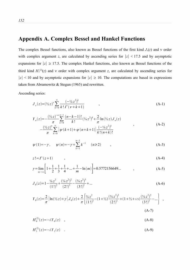
152
Appendix A. Complex Bessel and Hankel Functions
The complex Bessel functions, also known as Bessel functions of the first kind Jν(z) and ν order
with complex argument z, are calculated by ascending series for ∣z∣ < 17.5 and by asymptotic
expansions for ∣z∣ ≥ 17.5. The complex Hankel functions, also known as Bessel functions of the
third kind Hν(2)(z) and ν order with complex argument z, are calculated by ascending series for
∣z∣ < 10 and by asymptotic expansions for ∣z∣ ≥ 10. The computations are based in expressions
taken from Abramowitz & Stegun (1965) and rewritten.
Ascending series:
J ν z =½ z ν∑k=0
∞ ¼ z2k
k ! Γ νk1, (A-1)
Y n z =½ z n
π∑k=0
n1 nk1!k !
¼ z2k 2π
ln ½ z J n z
½ z n
π∑k=0
∞
{ψ k1ψ nk1} ¼ z2k
k !nk !
, (A-2)
ψ 1=γ , ψ n=γ ∑k=1
n1
k1 n2 , (A-3)
z !=Γ z1 , (A-4)
γ = limm∞ [11
21
31
4... 1
mln m]=0.5772156649... , (A-5)
J 0 z =1¼ z2
1!2¼ z22
2!2¼ z23
3!2... (A-6)
Y 0 z =2π
{ln ½ z γ }J 0 z 2π {¼ z2
1!21½ ¼ z22
2!21½1/3 ¼ z23
3!2...} ,
(A-7)
H 02 z =i Y 0 z , (A-8)
H 12 z =i Y 1 z . (A-9)

Appendix A. Complex Bessel and Hankel Functions 153
Asymptotic expansions:
J ν z = 2π z
{P ν , z cos χQ ν , z sin χ } , for ∣arg z∣π (A-10)
Y ν z = 2π z
{P ν , z sin χQ ν , z cos χ } for ∣arg z∣π (A-11)
H ν2 z = 2
π z{P ν , z i Q ν , z }ei χ for 2πarg zπ (A-12)
where χ=z 12
ν14π and, with 4ν2 denoted by µ,
P ν , z ≈∑k=0
∞
k ν ,2 k 2 z 2 k =1µ1µ9
2!8 z 2µ1µ9µ25µ49
4!8 z 4...
(A-13)
Q ν , z ≈∑k=0
∞
k ν , 2 k12 z 2 k1 =µ1
8 zµ1µ9µ25
3!8 z 3... , (A-14)
where Γ is the Euler's formula.

154
Appendix B. Algebraic formulation of Green's functions on
layered medium
The expressions for the general displacement field in cylindrical coordinates corresponding to
dynamic loads with disk, ring and point distributions acting on or within a layered medium reported
by Kausel & Peek (1982) are (see section 3.3.3 for nomenclature and geometry):
urmn={∑l=1
2 N
α Rnl φ x
ml dd r
f lRµ
r ∑l=1
N
α Lnl φ y
ml f lL}cos µθ
sin µθ (B-1)
uθmn={µ
r ∑l=1
2 N
α Rnl φ x
ml f lR∑
l=1
N
α Lnl φ y
ml dd r
f lL}sin µθ
cos µθ (B-2)
uzmn={∑l=1
2 N
α Rnl φ z
ml f lR k l}cos µθ
sin µθ (B-3)
where the corresponding variables can be taken from Tables 1 and 2.
TABLE 1
I 1 l=∫0
∞ 1k 2k l
2 J 0k r J 1k r0d k=
Im k l0 { π2 i k l
J 0k l r H 12k l r0
1r0 k l
2 0rr0
π2 i k l
J 1k l r0H 02k l r r0r }
I 2 l=∫0
∞ kk 2k l
2 J 1k r J 1k r0d k=
Im k l0 {π2 i
J 1k l r H 12k l r0 0rr0
π2 i
J 1k l r0H 12k l r r0r }
I 3 l=∫0
∞ 1k k 2k l
2J 1k r J 1k r0d k=
Im k l0 { π2 i k l
2 J 1r H 12k l r0
r2 r0 k l
2 0rr0
π2 i k l
2 J 1k l r0H 12k l r
r0
2 r k l2 r0r}

Appendix B. Algebraic formulation of Green's functions on layered medium 155
I 4 l=∫0
∞ kk 2k l
2 J 0k r J 0k r0d k=
Im k l0 {π2 i
J 0k l r H 02k l r0 0rr0
π2 i
J 0k l r0H 02k l r r0r }
Note:
I 1 l* r , r0=I 1 l r0 , r ; I 2 l=
d I 1 l
d r; I 1 l=
1r
I 3 ld
d rI 3 l ; I 4 l=
1r0
I 1 ld
d r0I 1 l=
1r
I 1 l* d
d rI 1 l
*
TABLE 2
Load Fourier index µ α Rn l α L
n l f l r
Horizontal disk 1 q r0 φ xn l q r0 φ y
n l I 3 l
Vertical disk 0 q r0 φ zn l 0
I 1 l
k l
Horizontal ring 1 r0 φ xn l r0 φ y
n l I 1 l*
Vertical ring 0 r0 φ zn l 0
I 4 l
k l
Horizontal point 1 P φ xn l /4 i P φ y
n l /4 iH 1
2
k l
Vertical point 0 P φ zn l /4 i 0
H 02
k l
n layer interface at which load is applied.
m layer interface at which displacements are desired.
r0 radius of the load
r horizontal distance from vertical axis of load center to the point where displacements are
computed.
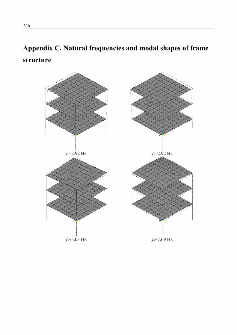
156
Appendix C. Natural frequencies and modal shapes of frame
structure
f1=2.92 Hz f2=2.92 Hz
f3=5.03 Hz f4=7.69 Hz

Appendix C. Natural frequencies and modal shapes of frame structure 157
f5=8.33 Hz f6=8.39 Hz
f7=15.02 Hz f8=15.02 Hz
f9=15.48 Hz f10=15.48 Hz