Embed Size (px)
Citation preview

University of Calgary
PRISM University of Calgarys Digital Repository
Graduate Studies The Vault Electronic Theses and Dissertations
2015-02-04
Reduction of Wellbore Positional Uncertainty During
Directional Drilling
Hadavand Zahra
Hadavand Z (2015) Reduction of Wellbore Positional Uncertainty During Directional Drilling
(Unpublished masters thesis) University of Calgary Calgary AB doi1011575PRISM27569
httphdlhandlenet110232082
master thesis
University of Calgary graduate students retain copyright ownership and moral rights for their
thesis You may use this material in any way that is permitted by the Copyright Act or through
licensing that has been assigned to the document For uses that are not allowable under
copyright legislation or licensing you are required to seek permission
Downloaded from PRISM httpsprismucalgaryca
UNIVERSITY OF CALGARY
Reduction of Wellbore Positional Uncertainty During Directional Drilling
by
Zahra Hadavand
A THESIS
SUBMITTED TO THE FACULTY OF GRADUATE STUDIES
IN PARTIAL FULFILMENT OF THE REQUIREMENTS FOR THE
DEGREE OF MASTER OF SCIENCE
GRADUATE PROGRAM IN GEOMATICS ENGINEERING
CALGARY ALBERTA
JANUARY 2015
copy Zahra Hadavand 2015
Abstract
Magnetic measurement errors significantly affect the wellbore positional accuracy in
directional drilling operations taken by Measurement While Drilling (MWD) sensors Therefore
this research has provided a general overview of error compensation models for magnetic
surveys and elaborated the most accurate calibration methods of hard- and soft-iron as well as
multiple-survey correction for compensating drilling assembly magnetic interference to solve the
problem of wellbore positional uncertainty and provide accurate surveying solution downhole
The robustness of hard- and soft-iron calibration algorithm was validated through an iterative
least-squares estimator initialized using a two-step linear solution A case study of a well profile
a simulated well profile and a set of experimental data are utilized to perform a comparison
study The comparison analysis outcomes imply that position accuracy gained by multistation
analysis surpasses hard- and soft-iron compensation results Utilization of multiple-survey
correction in conjunction with real-time geomagnetic referencing to monitor geomagnetic
disturbances such as diurnal effects as well as changes in the local field by providing updated
components of reference geomagnetic field provide superior accuracy
ii
Acknowledgements
I would like to express my gratitude to my supervisors Dr Michael Sideris and Dr Jeong
Woo Kim for their support on this research project over the past two and a half years
I am deeply thankful to my supervisor Dr Sideris for his professional supervision critical
discussions guidance and encouragements
I would like also to thank Dr Kim my co-supervisor for proposing this research project for
his continuous support and immeasurable contributions throughout my studies I would like to
thank Dr Kim for the time he offered to facilitate this research project by providing access to the
surveying equipment available at the Laboratory of the Department of Geomatics Engineering at
the University of Calgary
I thank the students in the Micro Engineering Dynamics and Automation Laboratory in
department of Mechanical amp Manufacturing Engineering at the University of Calgary for the
collection of the MEMS sensors experimental data
I would thank Dr Simon Park and Dr Mohamed Elhabiby for serving on my examination
committee I am really thankful of Department of Geomatics Engineering University of Calgary
for the giving me the chance to pursue my studies in the Master of Science program
iii
Dedication
To my father and my mother for their unlimited moral support and continuous
encouragements
You have been a constant source of love encouragement and inspiration
ldquoWords will never say how grateful I am to yourdquo
iv
Table of Contents
Abstract ii Acknowledgements iii Dedication iv Table of Contentsv List of Tables vii List of Symbols and Abbreviations xi
CHAPTER ONE INTRODUCTION1 11 Problem statement3
111 Borehole Azimuth Uncertainty3 112 Geomagnetic Referencing Uncertainty 5
12 Thesis Objectives 6 13 Thesis Outline 7
CHAPTER TWO REVIEW OF DIRECTIONAL DRILLING CONCEPTS AND THEORY 8
21 Wellbore Depth and Heading 8 22 Review of Sources and Magnitude of Geomagnetic Field Variations9
221 Review of Global Magnetic Models10 222 Measuring Crustal Anomalies Using In-Field Referencing (IFR) Technique 11 223 Interpolated IFR (IIFR) 12
23 Theory of Drillstring Magnetic Error Field 13 24 Ferromagnetic Materials Hard-Iron and Soft-Iron Interference 14 25 Surveying of Boreholes 15 26 Heading Calculation 17 27 Review of the Principles of the MWD Magnetic Surveying Technology21 28 Horizontal Wells Azimuth 22 29 Previous Studies24
291 Magnetic Forward Modeling of Drillstring25 292 Standard Method 25 293 Short Collar Method or Conventional Magnetic Survey (Single Survey) 26 294 Multi-Station Analysis (MSA) 28 295 Non-Magnetic Surveys 30
210 Summary30
CHAPTER THREE METHODOLOGY 32 31 MSA Correction Model 32 32 Hard-Iron and Soft-Iron Magnetic Interference Calibration38
321 Static Hard-Iron Interference Coefficients 38 322 Soft-Iron Interference Coefficients39 323 Relating the Locus of Magnetometer Measurements to Calibration Coefficients
40 324 Calibration Model41 325 Symmetric Constrait 44 326 Least-Squares Estimation 47
v
327 Establishing Initial Conditions 51 3271 Step 1 Hard-Iron Offset estimation51 3272 Step 2 Solving Ellipsoid Fit Matrix by an Optimal Ellipsoid Fit to the Data
Corrected for Hard Iron Biases 52 33 Well path Design and Planning 54 34 Summary58
CHAPTER FOUR RESULTS AND ANALYSIS60 41 Simulation Studies for Validation of the Hard and Soft-Iron Iterative Algorithm60 42 Experimental Investigations 70
421 Laboratory Experiment70 4211 Experimental Setup70 4212 Turntable Setup72 4213 Data Collection Procedure for Magnetometer Calibration 73
422 Heading Formula 74 423 Correction of the Diurnal Variations 75 424 Calibration Coefficients79
43 Simulated Wellbore 84 44 A Case Study 95 45 Summary101
CHAPTER FIVE CONCLUSIONS AND RECOMMENDATIONS FOR FUTURE RESEARCH103
51 Summary and Conclusions 103 52 Recommendations for Future Research106
521 Cautions of Hard-Iron and Soft-iron Calibration 106 522 Cautions of MSA Technique 107
REFERENCES 110
APPENDIX A SIMULATED WELLBORE116
vi
List of Tables
Table 4-1 The ellipsoid of simulated data 62
Table 4-2 Parameters solved for magnetometer calibration simulations 65
Table 4-3 Features of 3-axis accelerometer and 3-axis magnetometer MEMS based sensors 71
Table 4-4 Turn table setup for stationary data acquisition 73
Table 4-5 Diurnal correction at laboratory 79
Table 4-6 Parameters in the magnetometer calibration experiment 80
Table 4-7 A comparative summary of headings calibrated by different methods with respect to the nominal heading inputs 83
Table 4-8 Geomagnetic referencing values applied for the simulated wellbore 86
Table 4-9 The ellipsoid of simulated data 87
Table 4-10 Calibration parameters solved for simulated wellbore 89
Table 4-11 Comparative wellbore trajectory results of all correction methods 94
Table 4-12 Geomagnetic referencing values 95
Table 4-13 Calibration parameters solved for the case study 96
Table 4-14 Comparative wellbore trajectory results of all correction methods 100
vii
List of Figures and Illustrations
Figure 2-1 Arrangement of sensors in an MWD tool 8
Figure 2-2 A Perspective view of Earth-fixed and instrument-fixed orthogonal axes which denote BHA directions in three dimensions 16
Figure 2-3 Horizontal component of error vector 24
Figure 2-4 Eastwest component of error vector 24
Figure 2-5 Conventional correction by minimum distance 29
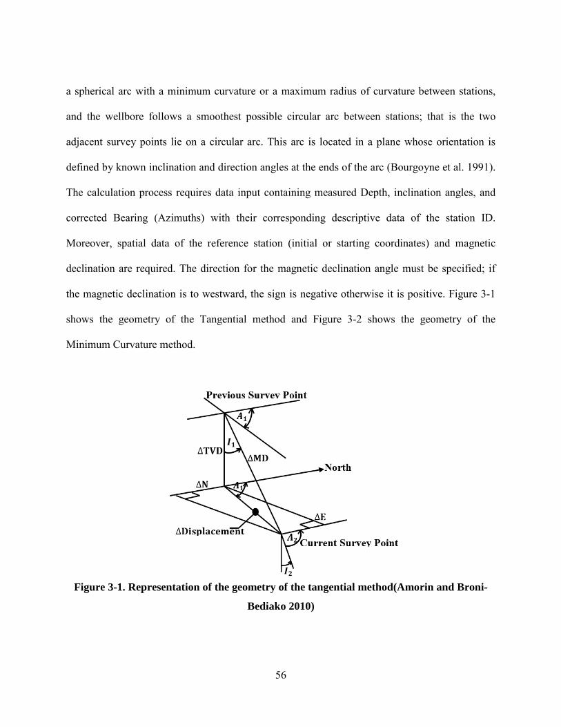
Figure 3-1 Representation of the geometry of the tangential method 56
Figure 3-2 Representation of the geometry of the minimum curvature method 57
Figure 4-1 Sphere locus with each circle of data points corresponding to magnetic field measurements made by the sensor rotation at highside 90deg 61
Figure 4-2 Sphere locus with each circle of data points corresponding to magnetic field measurements made by the sensor rotation at inclination 90deg 62
Figure 4-3 A schematic illustrating the disturbed data lying on an ellipsoid 63
Figure 4-4 Histogram of the magnetometer output error based on real data of a case study 64
Figure 4-5 Case I Parameters of hard-iron (in mGauss) and soft-iron (unit-less) for the least-squares iterations 67
Figure 4-6 Case II Parameters of hard-iron (in mGauss) and soft-iron (unit-less) for the least-squares iterations 68
Figure 4-7 Case III Parameters of hard-iron (in mGauss) and soft-iron (unit-less) for the least-squares iterations 68
Figure 4-8 Case IV Divergence of hard-iron (in mGauss) and soft-iron (unit-less) estimates for the least-squares iterations 69
Figure 4-9 Case V Divergence of hard-iron (in mGauss) and soft-iron (unit-less) estimates for the least-squares iterations 69
Figure 4-10 Case VI Parameters of hard-iron (in mGauss) and soft-iron (unit-less) for the least-squares iterations 70
Figure 4-11 Experimental setup of MEMS integrated sensors on turn table at 45deg inclination 74
Figure 4-12 Inclination set up for each test 75
viii
Figure 4-13 The observations of the geomagnetic field strength follow a 24 hour periodic trend 77
Figure 4-14 Geomagnetic field intensity in the frequency domain 78
Figure 4-15 Geomagnetic field intensity in the time domain 79
Figure 4-16 Portion of the ellipsoid representing the locus of magnetometer measurements from laboratory experimental data 81
Figure 4-17 Headings calibrated by MSA versus hard and soft iron (georeferncing obtained by IGRF model corrected for diurnal effects) 82
Figure 4-18 Headings calibrated by MSA versus hard and soft iron (georeferncing obtained by IGRF model without diurnal corrections) 82
Figure 4-19 Simulated wellbore horizontal profile 85
Figure 4-20 Portion of the ellipsoid representing the locus of magnetometer measurements from BUILD section of the simulated wellbore 87
Figure 4-21 Portion of the ellipsoid representing the locus of magnetometer measurements from LATERAL section of the simulated wellbore 88
Figure 4-22 Conventional correction is unstable in LATERAL section 90
Figure 4-23 Conventional correction instability based on inclination 90
Figure 4-24 Calculated field strength by calibrated measurements 91
Figure 4-25 Calculated field direction by calibrated measurements 92
Figure 4-26 Case I Wellbore pictorial view of the simulated wellbore in horizontal plane (no error) 92
Figure 4-27 Case II Wellbore pictorial view of the simulated wellbore in horizontal plane (random normally distributed noise of 03 mGauss) 93
Figure 4-28 Case III Wellbore pictorial view of the simulated wellbore in horizontal plane (random normally distributed noise of 6 mGauss) 93
Figure 4-29 Conventional correction is unstable in LATERAL section 97
Figure 4-30 Zoom1 of Figure 4-29 97
Figure 4-31 Zoom2 of Figure 4-29 98
Figure 4-32 Conventional correction instability based on inclination 98
ix
Figure 4-33 Calculated field strength by calibrated measurements 99
Figure 4-34 Calculated field direction by calibrated measurements 99
Figure 4-35 Wellbore pictorial view in horizontal plane by minimum curvature 102
x
Symbol
AZ
1198601198851
1198601198852
B
B
BP
BN BE BV
BV(119899) Bh(119899)
BV(ref) Bh(ref)
Bx By and Bz
BxCorr(119899) ByCorr(119899) BzCorr(119899)
Bxm(119899) Bym(119899) Bzm(119899)
DIP
DL
g
List of Symbols and Abbreviations
Description
borehole azimuth
azimuth angle at upper survey point
azimuth angle at lower survey point
geomagnetic vector
strength of geomagnetic field
magnetic field measured at a survey point
geomagnetic components along Earthrsquos coordinate frame
vertical and horizontal components of magnetic field at 119899P
th
survey station
reference value of vertical and horizontal components of
geomagnetic field
geomagnetic components along instrument-fixed coordinate
frame
corrected magnetic components at 119899P
th survey station in
instrument-fixed coordinate frame
measured magnetic components at 119899P
th survey station in
instrument-fixed coordinate frame
dip angle of geomagnetic vector
ldquodog-legrdquo curvature
magnitude of gravity vector
xi
g gravity vector
Gx Gy Gz gravity components along instrument-fixed coordinate frame
HS borehole highside angle
I borehole inclination
1198681 inclination angle at upper survey point
1198682 inclination angle at lower survey point
MD measured depth
N number of surveys
RF ratio factor for minimum curvature
TVD true vertical depth
unit vectors in Earthrsquos coordinate frame UNEV
unit vectors in instrument-fixed coordinate frame UXYZ
V hard-iron vector
components of hard-iron vector along instrument-fixed Vx Vy and Vz
coordinate frame
W soft-iron matrix
∆ change in parameter
∆119860119885 borehole azimuth error
∆Bx ∆By drillstring magnetic error field in cross-axial direction
∆Bz drillstring magnetic error field in axial direction
εx εy εz small perturbations of ∆Bx ∆By ∆Bz
119985 variance
xii
Abbreviation Description
BGGM British Global Geomagnetic Model
BHA Bottom-Hole-Assembly
HDGM High Definition Geomagnetic Model
IFR In-Field Referencing
IGRF International Geomagnetic Reference Field
IIFR Interpolated IFR
MEMS Micro Electro-Mechanical Systems
mGauss miliGauss
MSA Multi-Station Analysis
MWD Measurement While Drilling
NMDC Non-Magnetic Drill Collars
NOAA National Oceanic and Atmospheric Administration
nT nanoTesla
SSA Single Station Analysis
WBM Wellbore Mapping
xiii
Chapter One Introduction
Directional drilling is the technology of directing a wellbore along a predefined trajectory
leading to a subsurface target (Bourgoyne et al 2005) In recent years directional drilling
technology has gained more attention than vertical drilling in global oil and gas industries The
reason is that horizontal (deviated) wells whose borehole intentionally departs from vertical by a
significant extent over at least part of its depth (Russell and Russell 2003) have higher oil and
gas deliverability since they have larger contact area with oil and gas reservoirs (Joshi and Ding
1991) This in turn significantly reduces the cost and time of drilling operation since a cluster of
deviated wells drilled from a single drilling rig allows a wider area to be tapped at one time
without the need for relocation of the rig which is expensive and time-consuming Therefore
drilling horizontal wells can reduce the number of wells required and minimize surface
disturbance which is important in environmentally sensitive areas However suitable control of
the borehole deviation as it is drilled requires precise knowledge of the instantaneous depth and
heading of the wellbore Therefore obtaining accurate measurements of depth inclination and
azimuth of wellbore is a fundamental requirement for the drilling engineer to be all the time
aware of the drilling bit direction
Depth is acquired by drill pipe measurements while inclination and azimuth are achieved
from gravitational and magnetic field measurements Horizontal drilling operations in the oil
industry utilize the measurement while drilling (MWD) technique MWD incorporates a package
of sensors including a tri-axial magnetometer and a tri-axial accelerometer mounted in three
mutually orthogonal directions inserted within a downhole probe The sensors monitor the
position and the orientation of the bottom-hole-assembly (BHA) during drilling by instantaneous
measuring of magnetic and gravity conditions while the BHA is completely stationary
1
A perpendicular pair or an orthogonal triad of accelerometers measure the Earthrsquos gravity
field to determine the BHA inclination and tool face angles while the magnetometers measure
the geomagnetic components to determine the BHA azimuth at some predetermined survey
stations along the wellbore path
In a directional survey of wellbore many sources of uncertainty can degrade accuracy
including gravity model errors depth errors sensor calibration instrument misalignment BHA
bending centralization errors and environmental magnetic error sources This thesis focuses on
the wellbore magnetic directional survey since the main difficulty in making an accurate
positional survey of wellbore is largely driven by uncertainty resulting from environmental
magnetic error sources which are caused by two major error sources the un-modeled
geomagnetic field variations and drillstring magnetism interference induced by ferrous and steel
materials around the drilling rig
The best insurance against the geomagnetic referencing uncertainty is a site survey to map the
crustal anomalies (local magnetic parameters) using In-Field Referencing (IFR) and remove
geomagnetic disturbances using the Interpolated IFR (IIFR) method Magnetic interference of
drilling assembly is compensated through various methods such as a multiple-survey correction
in order to reduce positional survey uncertainty
Reduced separation between adjacent wells is allowed as a result of the overall reduced
position uncertainty (Lowdon and Chia 2003) In recent years the oil companies and the drilling
contractors have shown a great deal of interest in research investigations of possible error
sources in directional drilling magnetic surveys
A drilling engineerrsquos ability to determine the borehole trajectory depends on the accumulation
of errors from wellhead to total path In modern magnetic surveys with MWD tools the
2
combined effects of accumulated error may reach values of 1 of the measured well depth
which could be unacceptably large for long wellbores (Buchanan et al 2013) To place wellbores
accurately when using MWD surveying tools the modern industry has promoted the
development of rigorous mathematical procedures for compensating various error sources As a
result the general wellbore positional accuracies available in the industry are of the order of
05 of the wellbore horizontal displacement
11 Problem statement
The Wellbore Positional accuracy in directional drilling operations taken by Measurement
While Drilling (MWD) sensors decreases with the increase of the inclination from the vertical
From experiments it is evident that at small inclinations the influence of the drilling assembly
interfering field in the azimuth can often be neglected while at high inclinations the error in the
azimuth is significant As a result horizontal wells which are frequently employed in the oil and
gas industry represent a challenge in directional surveying (Grindrod and Wolff 1983) This
study is concerned with the magnetic surveying of boreholes and relates more particularly but
not exclusively to determining the corrected azimuth of a horizontal well Several error sources
affect the accuracy of the magnetic surveys and can be summarized as follows
111 Borehole Azimuth Uncertainty
Since in conventional magnetic instruments the azimuth read by the compass is determined by
the horizontal component of the local magnetic field all magnetic surveys are subject to azimuth
uncertainty if the horizontal component of the local magnetic field observed by the instrument at
the borehole location is not aligned with the expected magnetic north direction whose declination
is obtained from main-field geomagnetic models or the IFR technique (Brooks et al 1998) The
sources of error in azimuth can be categorized as follows (Scott and MacDonald 1979)
3
(i) The massive amount of ferrous and steel materials around the drilling rig have a
deleterious impact on the magnetometer measurements taken by MWD sensors (Thorogood and
Knott 1990) Drilling assembly magnetic error field is a common phenomenon as there is a
desire to get the survey information as close to the bit as possible
(ii) The magnetic surveying sensors are installed at a distance behind the drill bit due to the
additional weight imposed by Non-Magnetic Drill Collars (NMDC) on the bit (Conti 1989)
Consequently Conti (1989) and Rehm et al (1989) have evaluated that the sensors might not be
capable of monitoring some rotational motions experienced only by the drill bit assembly and
thus the overall reliability of the magnetic survey is affected Another source of error in magnetic
surveys is misalignment of the survey toolrsquos axis with the borehole axis The cause of this could
be bending of the drill collars within the borehole or poor centralization of the tool within the
drill collar (Carden and Grace 2007) The azimuth errors caused by instrument misalignment are
usually small in comparison with others and their effect tends to be randomized as the toolface
angle changes between surveys (Brooks et al 1998)
(iii) Sensor calibration errors which are the errors in accelerometer and magnetometer
readings (and gyro readings) cause the measurements to be imprecise and consequently there is
uncertainty in the azimuth calculated from these measurements (Brooks et al 1998) In this
study effects of temperature and pressure were considered negligible The calibration of the
magnetometer is more complicated because there are error sources not only from instrumentation
but also from the magnetic deviations on the probe which was classified as the first error source
above
4
112 Geomagnetic Referencing Uncertainty
The geomagnetic field declination is normally determined by estimations of the geomagnetic
field obtained from global and regional models of the main field such as the International
Geomagnetic Reference Field (IGRF) (Russell et al 1995) Russell et al (1995) indicated that
the geomagnetic field for any location at any time calculated only from a main-field model
includes significant error These models do not consider short term magnetic variations of
geologic sources and geomagnetic disturbances such as diurnal variations which are potentially
large and thus lead to considerable uncertainty in declination which is a major contributor to
azimuth uncertainty The best insurance against crustal anomalies is a site survey to measure the
local magnetic parameters in real-time using IFR in order to map the local anomalies as
corrections to one of the global models Diurnal variations can be corrected using IIFR method
Since variations of the geomagnetic field are quite significant with respect to the performance
capabilities of the magnetic survey tools geomagnetic referencing uncertainty raises a global
drilling problem whenever magnetic survey tools are employed (Wright 1988)
Cheatham et al (1992) and Thorogood (1990) have investigated that the declination
uncertainty and the drillstring magnetization interference associated with the surrounding
magnetic environment are systematic over a group of surveys and thus dominate the overall
uncertainty in the determination of wellbore orientation Recent trends in the drilling industry
tend to establish several horizontal wells from the same platform (Anon 1999 Njaerheim et al
1998) This necessitates the reduction of magnetic survey uncertainty by the utilization of a
reliable error model so as to correct the BHA position and orientation within the severe
downhole drilling conditions and avoid collision with adjacent wells
5
12 Thesis Objectives
Within the context of using magnetic error correction models for the purpose of reducing
wellbore position uncertainty the main research objectives are as follows
bull Execute multistation analysis as well as utilize hard and soft-iron algorithm for
calibration of magnetometers to compensate the drilling assembly magnetic disturbances through
real experimental and simulated results
bull Estimate the applicability of the magnetic compensation methods including single-
survey analysis multiple-survey analysis as well as hard- and soft-iron calibration by
comparative evaluation of respective results in order to be able to identify the most accurate
magnetic compensation solution for drilling assembly magnetic interference and reach the
desired target
bull Analyze experimental results to investigate whether there is a noticeable improvement in
survey accuracy when the effects of time varying disturbances of geomagnetic field such as
diurnal variations are reduced through adaptive filtering of the wellsite raw magnetic data It may
be implied that the position accuracy of all correction methods can be improved by mapping the
crustal magnetic field of the drilling area
bull Correct the case study wellbore trajectory by applying the most accurate magnetic
compensation solution for drillstring-induced interference and combine the results with real-
time geomagnetic referencing (accounting for the influence of the crustal field as well as
secular variations in the main magnetic field) Afterward the achieved positional accuracy is
compared with the available wellbore positional accuracy in the industry
6
13 Thesis Outline
Chapter 2 provides background information necessary for understanding the concepts
discussed in Chapter 3 and 4 Chapter 3 discusses the MSA correction model as well as the hard-
iron and soft-iron magnetic interference calibration model and examines the most accurate well
path planning method applied in the oil industry to achieve the corrected wellbore trajectory
Chapter4 evaluates the proposed methods through the results of a case study simulation analysis
and experimental investigations Finally Chapter 5 provides the main conclusions with respect to
the stated thesis objectives and also provides recommendations for future investigations
7
Chapter Two REVIEW of DIRECTIONAL DRILLING CONCEPTS and THEORY
21 Wellbore Depth and Heading
While the depth of the BHA can be determined from the surface simply by counting the
number of standard-length tubes coupled into the drillstring determination of the BHA heading
requires downhole measurements (Russell and Russell 2003) Russell et al (1978) denoted the
word ldquoheadingrdquo as the vertical direction and horizontal direction in which the BHA is pointing
The vertical direction is referred to as inclination and the horizontal direction is referred to as
azimuth The combination of inclination and azimuth at any point down the borehole is the
borehole heading at that point For the purpose of directional analysis any length of the borehole
path can be considered as straight The inclination at any point along the borehole path is the
angle of the instrumentrsquos longitudinal axis with respect to the direction of the Earthrsquos gravity
vector when the instrumental axis is aligned with the borehole path at that point In other words
inclination is the deviation of the longitudinal axis of the BHA from the true vertical Azimuth is
the angle between the vertical plane containing the instrument longitudinal axis and a reference
vertical plane which may be magnetically or gyroscopically defined (Figure 2-1 and Figure 2-2)
Figure 2-1 Arrangement of sensors in an MWD tool
8
This study is concerned with the measurement of the azimuth defined by a magnetic reference
vertical plane containing a defined magnetic north (Russell and Russell 1991) The horizontal
angle from the defined magnetic north clockwise to the vertical plane including the borehole axis
is hereafter simply referred to as azimuth When the defined magnetic north contains the
geomagnetic main field vector at the instrument location the corresponding azimuth referred to
as ldquoabsolute azimuthrdquo or ldquocorrected azimuthrdquo is the azimuth value required in directional
drilling process However in practice the measured local magnetic field is deviated from the
geomagnetic main field (Russell and Russell 2003) The process of estimating these magnetic
distorting errors and removing them from the magnetometer measurements is the subject of this
research
The azimuth of wellbore is measured from magnetic north initially but is usually corrected to
the geographic north to make accurate maps of directional drilling A spatial survey of the path
of a borehole is usually derived from a series of measurements of an azimuth and an inclination
made at successive stations along the path and the distance between these stations are accurately
known (Russell 1989)
22 Review of Sources and Magnitude of Geomagnetic Field Variations
The geomagnetic field at any location is defined in terms of three components of a vector
including the field strength the declination angle defined as the direction of the geomagnetic
north relative to geographic (true) north and the dip angle defined as the dip angle of the
geomagnetic vector measured downwards from the horizontal (University of Highlands and
Island 2012) According to Wright (1988) and Ripka (2001) the geomagnetic field is used as a
north reference from which the wellbore direction is computed Afterward the geomagnetic
north is referenced to the geographic north form a knowledge of the declination angle A
9
knowledge of the sources and magnitude of geomagnetic field variations helps our understanding
of the magnetic survey accuracy problem A concise description of the geomagnetic field is
therefore appropriate here The geomagnetic field at any point on the Earthrsquos surface is the result
of the principal sources of magnetism as follows
(i) The main field originating from the enormous magnetic core at the heart of the Earth
accounts for about 98-99 of the field strength at most places at most times
(ii) The Earthrsquos core field is not stationary and has been turbulent over the course of history
resulting in a magnetic vector that is constantly changing This change referred to as the
ldquosecularrdquo variation is very rapid in geological time scales
(iii) Diurnal magnetic field variations and magnetic storms are caused by varying solar wind
and electric currents flowing external to the Earthrsquos surface and interacting with the main field
(Wolf and deWardt 1981)
Fields created by the magnetization of rocks and minerals in the Earthrsquos crust typically found
in deep basement formations in the vicinity of drilling (crustal anomalies) (Bourgoyne et al
2005)
Geomagnetic field is a function of time and geographical location (Ozyagcilar 2012c) and can
be modeled with reasonable accuracy using the global geomagnetic reference field models
221 Review of Global Magnetic Models
In order to keep track of the ldquosecularrdquo variation (long wavelengths) in the magnetic field of
the Earth core several global magnetic models are maintained to provide prediction models
International organizations such as INTERMAGNET collate data from observatories scattered
throughout the world to model the intensity and attitude of the geomagnetic field (University of
Highlands and Island 2012) For instance every year the data is sent to the British Geological
10
Survey in Edinburg where this data is entered to a computer model called the British Global
Geomagnetic Model (BGGM)
Higher-order models take into account more localized crustal effects (short wavelengths) by
using a higher order function to model the observed variations in the Earth field (University of
Highlands and Island 2012) The lower order models such as the International Geomagnetic
Reference Field (IGRF) are freely accessible over the internet whereas the higher order models
require an annual license This research applies the IGRF model coefficients produced by the
participating members of the IAGA Working Group V-MOD (Finlay et al 2010) Geomagnetic
referencing is now a well-developed service and various techniques have been used in the
industry for the purpose of measuring and predicting the geomagnetic field at the wellsite
222 Measuring Crustal Anomalies Using In-Field Referencing (IFR) Technique
One significant source of error in the determination of the geomagnetic reference field is
crustal variations The global models can only resolve longer wavelength variations in the
geomagnetic field and cannot be expected to account for localized crustal anomalies (University
of Highlands and Island 2012) In order to correct for the crustal anomalies the geomagnetic
field has to be measured on site IFR is the name given to the novel technique of measuring the
local geomagnetic field elements including field strength dip angle and declination in real-time
routinely made at magnetic observatories in the vicinity of the drilling activity while the
interference from the rig and drilling hardware and other man-made sources of magnetic
interference should be avoided
The field strength is measured by a Caesium or proton precision magnetometer Declination
and dip angle measurements are made by a non-magnetic theodolite with a fluxgate
magnetometer mounted on its telescope The measurement of declination angle is made against a
11
true north The true north can be determined by means of astronomical observations or by using
a high-accuracy north-seeking gyro mounted on the theodolite (Russell et al 1995) Once the
IFR measurements of the geomagnetic field have been taken contoured maps and digital data
files are produced and can be viewed with a computer software This allows the MWD contractor
to view the data and interpolate suitable geomagnetic field values at any point within the oilfield
(University of Highlands and Island 2012)
The crustal corrections vary only on geological time scales and therefore can be considered as
fixed over the lifetime of the field On the other hand the global model (such as IGRF) tracks
very well the time variation in the overall geomagnetic field As a result combining the global
model and the IFR crustal corrections provide the MWD contractor with the most accurate
estimate of the geomagnetic field at the rig (University of Highlands and Island 2012)
IFR significantly reduces declination uncertainty and improves the accuracy of magnetic
surveys by monitoring changes in the local geomagnetic field during surveys and therefore
providing updated components of the reference field (Russell et al 1995)
223 Interpolated IFR (IIFR)
IIFR is a method of correcting for time variant disturbances of the geomagnetic field in a way
that a reference station is installed on the surface at or near the wellsite to sense geomagnetic
disturbances such as diurnal variations (Lowdon and Chia 2003) The variations observed at this
surface reference station can be applied to the downhole data which will experience similar
variation (University of Highlands and Island 2012)
Experimental results have shown that time-variable disturbances experienced by observatories
even a long way apart follow similar trends The comparison of the observations made at a fixed
observatory with derived observations interpolated from other observatories several hundreds of
12
kilometers away from the drill site show a good match The data are interpolated from one or
more locations to another The readings observed at the nearby stations are effectively weighted
by the proximity to the drill site
This is not always practical and requires a magnetically clean site with power supply nearby
and some method of transmitting the data in real-time from the temporary observatory
(University of Highlands and Island 2012) IIFR is a patented method and can be used under
license from the inventors (Russell et al 1995)
23 Theory of Drillstring Magnetic Error Field
The measurements of magnetic vectors are susceptible to distortion arising from inherent
magnetism of ferrous materials incorporated in the drillstring and BHA (Cheatham et al 1992)
By convention this magnetic field interference is divided into remnant hard-iron offset and
induced soft-iron distortions
At the bit and above and below the sensors the magnetic flux is forced to leave the steel ie
magnetic poles occur at the ends of the steel sections which construct a dipole A magnetic error
field is produced by the dipole at the compass location This magnetic error field will interact
with the Earthrsquos total field to produce a resultant field The compass will respond to the
horizontal component of the resultant field (Scott and MacDonald 1979)
Drillstring magnetic error field in the axial direction ∆B119911 exceeds the cross axial magnetic
error field The reason is that the ferromagnetic portions of the drillstring are displaced axially
from the instrument (Brooks 1997) and the drillstring is long and slender and is rotated in the
geomagnetic field (Brooks 1997)
13
24 Ferromagnetic Materials Hard-Iron and Soft-Iron Interference
Iron cobalt nickel and their alloys referred to as ferromagnets can maintain permanent
magnetic field and are the predominant sources to generate static hard-iron fields on the probe in
the proximity of the magnetometers Static hard-iron biases are constant or slowly time-varying
fields (Ozyagcilar 2012c) The same ferromagnetic materials when normally unmagnetized and
lack a permanent field will generate their own magnetic field through the induction of a
temporary soft-iron induced magnetization as they are repeatedly strained in the presence of any
external field whether the hard-iron or the geomagnetic field during drilling operations
(Ozyagcilar 2012b) In the absence of the external field there is no soft-iron field (Ozyagcilar
2012c) This generated field is affected by both the magnitude and direction of the external
magnetic field In a moving vehicle the orientation of the geomagnetic field relative to the
vehicle changes continuously Thus the resulting soft-iron errors are time varying
The ability of a material to develop an induced soft-iron field in response to an external field
is proportional to its relative magnetic permeability Magnetic interference can be minimized by
avoiding materials with high relative permeability and strongly magnetized ferromagnetic
components wherever possible and selecting alternatives and also placing the magnetometer as
far away as possible from such components (Brooks et al 1998)
The geomagnetic field is distorted by the hard-iron and soft-iron interference and the
magnetometer located in the vicinity of the magnets will sense the sum of the geomagnetic field
permanent hard-iron and induced soft-iron field and will compute an erroneous azimuth
(Ozyagcilar 2012c) The magnitude of hard-iron interference can exceed 1000120583119879 and can
saturate the magnetometer since the operating range of the magnetometer cannot accommodate
the sum of the geomagnetic and interference fields Thus in practice it is essential to accurately
14
estimate and subtract the hard-iron offset through correction methods of drilling assembly
corrupting magnetic field
25 Surveying of Boreholes
The heading measurements are made using three accelerometers which are preferably
orthogonal to one another and are set up at any suitable known arrangement of the three
orthogonal axes to sense the components of the Earthrsquos gravity in the same three mutually
orthogonal directions as the magnetometers sense the components of the local magnetic field
(Helm 1991) The instrumentation sensor package including accelerometers and magnetometers
is aligned in the survey toolrsquos coordinate system with the orthogonal set of instrument-fixed
axes so that these three orthogonal axes define the alignment of the instrumentation relative to
the BHA (Thorogood and Knott 1990) Since both the accelerometers and magnetometers are
fixed on the probe their readings change according to the orientation of the probe With three
accelerometers mounted orthogonally it is always possible to figure out which way is lsquodownrsquo
and with three magnetometers it is always possible to figure out which way is the magnetic
north
The set of Earth-fixed axes (N E V) shown in Figure 2-2 is delineated with V being in the
direction of the Earthrsquos gravity vector and N being in the direction of the horizontal component
of the geomagnetic main field which points horizontally to the magnetic north axis and the E
axis orthogonal to the V and N axes being at right angles clockwise in the horizontal plane as
viewed from above ie the E axis is an east-pointing axis The set of instrument-fixed axes (X
Y Z) is delineated with the Z axis lying along the longitudinal axis of the BHA in a direction
towards the bottom of the assembly and X and Y axes lying in the BHA cross-axial plane
15
perpendicular to the borehole axis while the Y axis stands at right angles to the X axis in a clock
wise direction as viewed from above
Figure 2-2 A Perspective view of Earth-fixed and instrument-fixed orthogonal axes which
denote BHA directions in three dimensions (modified from Russell and Russell 2003)
The set of instrument-fixed orthogonal axes (X Y Z) are related to the Earth-fixed set of axes
(N E V) through a set of angular rotations of azimuth (AZ) inclination (I) and toolface or
highside (HS) angles as shown in Figure 2-2 (for convenience of calculations a hypothetical
origin O is deemed to exist at the center of the sensor package) ldquoHSrdquo a further angle required
to determine the borehole orientation is a clockwise angle measured in the cross-axial plane of
borehole from a vertical plane including the gravity vector to the Y axis The transformation of a
16
unit vector observed in the survey toolrsquos coordinate system to the Earthrsquos coordinate system
enables the determination of the borehole orientation (Russell and Russell 2003)
At certain predetermined surveying stations while the BHA is completely stationary the
undistorted sensor readings of the gravity and magnetic field components measured along the
direction of the orthogonal set of instrument-fixed coordinate frame are denoted by (119866119909 119866119910 119866119911)
and (119861119909 119861119910 119861119911) respectively and are mathematically processed to calculate the corrected
inclination highside and azimuth of borehole along the borehole path at the point at which the
readings were taken The BHA position is then computed by assuming certain trajectory between
the surveying stations (Russell and Russell 1979)
These calculations which are performed by the computing unit of the drilling assembly are
well-known in the literature and were well discussed by different researchers Based on the
installation of orthogonal axes mentioned in this section Russell and Russell (1978) Russell
(1987) and Walters (1986) showed that the inclination (I) the highside (HS) and the azimuth
(AZ) can be determined as discussed below
26 Heading Calculation
The transformation between unit vectors observed in the survey toolrsquos coordinate system (X
Y Z) and the Earthrsquos coordinate system (N E V) is performed by the vector Equation (21)
U119873119864119881 = 120546119885 119868 119867119878 U119883119884119885 (21)
where 119880119873 119880119864 and 119880119881 are unit vectors in the N E and V directions 119880119883 119880119884 and 119880119885 are unit
vectors in the X Y and Z directions respectively and 120546119885 119868 119867119878 represent the rotation
matrices according to Russell and Russell (1978)
cos 119860119885 minussin 119860119885 0 119860119885 = sin 119860119885 cos 119860119885 0 (22)
0 0 1 17
cos 119868 0 sin 119868 119868 = 0 1 0 (23)
minussin 119868 0 cos 119868
cos 119867119878 minus sin 119867119878 0 119867119878 = sin 119867119878 cos 119867119878 0 (24)
0 0 1
The vector operation for a transformation in the reverse direction can be written as
= 119880 119883119884119885 119867119878119879 119868 119879 120546119885T UNEV (25)
The first step is to calculate the borehole inclination angle and highside angle Operating the
vector Equation (25) on the Earthrsquos gravity vector results in Equation (26)
119866119909 cos 119867119878 sin 119867119878 0 cos 119868 0 minus sin 119868 cos 119860119885 sin 119860119885 0 0 119866119910 = minus sin 119867119878 cos 119867119878 0 0 1 0 minussin 119860119885 cos 119860119885 0 0 (26 ) 119866119911 0 0 1 sin 119868 0 cos 119868 0 0 1 g
where g is the magnitude of gravity derived as the square root of the sum of the individual
squares of gravity vector and the gravity vector is defined as
g = g 119880119881 = 119866119909 119880119883 + 119866119910 119880119884 + 119866119911 119880119885 (27)
It is assumed that the probe is not undergoing any acceleration except for the Earthrsquos gravity
field In the absence of external forces in static state the accelerometer experiences only the
Earth gravity with components 119866119909 119866119910 119866119911 which are therefore a function of the gravity
magnitude and the probe orientation only This study is also based on the assumption that the
gravity measurements 119866119909 119866119910 and 119866119911 are substantially identical to the respective actual Earthrsquos
gravity field (because accelerometers are not affected by magnetic interference) Equations (28)
through (210) provide gravity field components in the (X Y Z) frame
119866119909 = minusg cos 119867119878 sin 119868 (28)
119866119910 = g sin 119868 sin 119867119878 (29)
18
119866119911 = g cos 119868 (210)
Thus the highside angle HS can be determined from
119866119910tan 119867119878 = (211) minus119866119909
The inclination angle can be determined from
2Gx2 + Gysin 119868 (212)
cos 119868 =
Gz
Or
Gzcos 119868 = (213) 2Gx2 + Gy2 + Gz
Based on the above equations it is obvious that the inclination and highside angles are
functions of only the gravity field components
The next step is to calculate the borehole azimuth The vector expression of the geomagnetic
field in Earth-fixed and instrument-fixed frames are denoted as
119861 = 119861119873 119880119873 + 119861119864 119880119864 + 119861119881 119880119881 = 119861119909 119880119883 + 119861119910 119880119884 + 119861119911 119880119885 (214)
where 119861119873 119861119864 and 119861119881 are the geomagnetic field components in (N E V) frame Operating the
vector Equation (21) on the magnetic field vector results in Equation (215)
119861119873 B cos(DIP)119861119864 = 0 119861119881 B sin(DIP)
cos 119860119885 minus sin 119860119885 0 cos 119868 0 sin 119868 cos 119867119878 minussin 119867119878 0 119861119909= sin 119860119885 cos 119860119885 0 0 1 0 sin 119867119878 cos 119867119878 0 119861119910 (215)
0 0 1 minussin 119868 0 cos 119868 0 0 1 119861119911
19
2 12where strength of geomagnetic field B is obtained as 1198611198732 + 119861119881 DIP is the dip angle
of the geomagnetic vector measured downwards from the horizontal There is no requirement to
know the details of B or the DIP in order to calculate the azimuth since these cancel in the angle
calculations Equation (215) yields magnetic field components in the (N E V) frame as follows
119861119873 = cos 119860119885 cos 119868 119861119909 cos 119867119878 minus 119861119910 sin 119867119878 + 119861119911 sin 119868
minus sin 119860119885 119861119909 sin 119867119878 + 119861119910 cos 119867119878 (216)
119861119864 = sin 119860119885 cos 119868 119861119909 cos 119867119878 minus 119861119910 sin 119867119878 + 119861119911 sin 119868
+ cos 119860119885 119861119909 sin 119867119878 + 119861119910 cos 119867119878 (217)
119861119881 = minussin 119868 119861119909 cos 119867119878 minus 119861119910 sin 119867119878 + 119861119911 cos 119868 (218)
The calculated azimuth at the instrument location is the azimuth with respect to the Earthrsquos
magnetic north direction if the local magnetic field vector measured at the instrument location is
solely that of the geomagnetic field (Russell and Russell 1979) Under this condition the
equations here ignore any magnetic field interference effects thus 119861119864 is zero and then the
azimuth is derived from Equation (217) by
sin 119860119885 minus 119861119909 sin 119867119878 + 119861119910 cos 119867119878 (219)
cos 119860119885 =
cos 119868 119861119909 cos 119867119878 minus 119861119910 sin 119867119878 + 119861119911 sin 119868
The azimuth angle is derived as a function of the inclination angle the highside angle and the
magnetic field components 119861119909 119861119910 and 119861119911 Therefore the azimuth is a function of both the
accelerometer and magnetometer measurements Substituting the above inclination and highside
equations into the above azimuth equation results in the following equation which is used to
20
convert from three orthogonal accelerations and three orthogonal magnetic field measurements
to the wellbore azimuth
119861119909 119866119910 minus 119861119910 119866119909 1198661199092 + 1198661199102 + 1198661199112sin 119860119885 (220)
cos 119860119885 = 119866119911 119861119909 119866119909 +119861119910 119866119910 + 119861119911 1198661199092 + 1198661199102
If the X-Y plane of the body coordinate system is level (ie the probe remains flat) only the
magnetometer readings are required to compute the borehole azimuth with respect to magnetic
north using the arctangent of the ratio of the two horizontal magnetic field components (Gebre-
Egziabher and Elkaim 2006)
By119860119885 = minustanminus1 (221) Bx
In general the probe will have an arbitrary orientation and therefore the X-Y plane can be
leveled analytically by measuring the inclination and highside angles of the probe (Gebre-
Egziabher and Elkaim 2006)
Post analysis of the results made by Russell and Russell (1978) showed that the coordinate
system of the sensor package (instrument-fixed coordinate system) may be set up at any suitable
known arrangements of the three orthogonal axes and different axes arrangements lead to
different azimuth formulas (Helm 1991) Therefore care should be taken when reading raw data
files and identifying the axes
27 Review of the Principles of the MWD Magnetic Surveying Technology
Conti et al (1989) showed that the directional drilling process should include MWD
equipment in addition to the conventional drilling assembly The well is drilled according to the
designed well profile to hit the desired target safely and efficiently Information about the
location of the BHA and its direction inside the wellbore is determined by use of an MWD tool
21
(Bourgoyne et al 2005) In current directional drilling applications the MWD tool incorporates a
package of sensors which includes a set of three orthogonal accelerometers and a set of three
orthogonal magnetometers inserted within a downhole probe to take instantaneous measurements
of magnetic and gravity conditions at some predetermined survey stations along the wellbore
path (with regular intervals of eg 10 m) while the BHA is completely stationary (Thorogood
1990)
In addition the MWD tool contains a transmitter module that sends these measurement data
to the surface while drilling Interpretation of this downhole stationary survey data provides
azimuth inclination and toolface angles of the drill bit at a given measured depth for each
survey station Coordinates of the wellbore trajectory can then be computed using these
measurements and the previous surveying station values for the inclination azimuth and
distance (Thorogood 1990)
The accelerometer measurements are first processed to compute the inclination and toolface
angles of the drill bit The azimuth is then determined using the computed inclination and
toolface angles and the magnetometer measurements (Russell and Russell 1979) Present MWD
tools employ fluxgate saturation induction magnetometers (Bourgoyne et al 2005)
After completing the drilling procedure wellbore mapping (WBM) of the established wells is
performed for the purpose of quality assurance WBM determines the wellbore trajectory and
direction as a function of depth and compares it to the planned trajectory and direction
(Bourgoyne et al 2005)
28 Horizontal Wells Azimuth
The borehole inclination is determined by use of the gravitational measurements alone while
the borehole azimuth is determined from both the gravitational and magnetic measurements
22
Since the accelerometers are not affected by magnetic interference inclination errors are very
small compared to azimuth errors On the other hand the calculation of borehole azimuth is
especially susceptible to magnetic interference from the drilling assembly
The drillstring magnetic error field does not necessarily mean an azimuth error will occur
Grindrod and Wolff (1983) proved that no compass error results from a vertical assembly or one
which is drilling in north or south magnetic direction The reason is as follows
(i) The conventional magnetic compass placed near the magnetic body aligns itself
according to the horizontal component of the resultant field produced from interaction of the
Earthrsquos total field and the error field of the magnetic body interference This resultant field is the
vectorial sum of the geomagnetic field and the drillstring error field (Grindrod and Wolff 1983)
(ii) It was mathematically proved that drillstring magnetic error field in axial direction
exceeds cross axial direction
Therefore simple vector addition in Equation (222) shows that the azimuth error equals the
ratio of the east-west component of the drillstring error vector and the Earthrsquos horizontal field as
shown in Figure 2-3 and Figure 2-4
∆B119911 sin 119868 sin 119860119885∆119860119885 = (222)
B cos(DIP)
where
∆119860119885 = Borehole Azimuth error ∆Bz= drillstring magnetic error field in axial direction
119868 = Borehole inclination AZ= Borehole azimuth
DIP= dip angle of geomagnetic vector |B| = Strength of geomagnetic field
∆Bz sin 119868 = Horizontal component of the drillstring error vector
∆Bz sin 119868 sin 119860119885 = EastWest component of the drillstring error vector
23
BN = B cos(DIP) = Horizontal component of geomagnetic field
However as the borehole direction and inclination change errors will occur This means that
the compass azimuth error increases with borehole inclination and also with a more easterly or
westerly direction of the borehole Therefore the azimuth uncertainty will particularly occur for
wells drilled in an east-west direction (Grindrod and Wolff 1983)
Figure 2-3 Horizontal component of error vector (modified from Grindrod and Wolff
1983)
Figure 2-4 Eastwest component of error vector (modified from Grindrod and Wolff 1983)
29 Previous Studies
24
The problem of drilling assembly magnetic interference has been investigated extensively in
the literature An overview of different methods that can be implemented for the correction of
this corrupting magnetic error field is provided here
291 Magnetic Forward Modeling of Drillstring
The magnitude of error field ∆119861119911 produced by the drillstring cylinder is modeled by a dipole
moment along the axis of the cylinder The application of classical magnetic theory together
with a better understanding of the changes in the magnetic properties of the drilling assembly as
drilling progresses provides a knowledge of magnetic moment size and direction of error field
which enables us to make good estimates of the drilling assemblyrsquos magnetic effects on the
survey accuracy for the particular geographic location (Scott and MacDonald 1979)
Scott and MacDonald (1979) made use of field data from a magnetic survey operation to
investigate magnetic conditions and proposed a procedure for quantifying magnetic pole strength
changes during drilling The strength of a magnetic pole is defined as equal to the magnetic flux
that leaves or enters the steel at the pole position (Grindrod and Wolff 1983) It is noted that the
pole strengths are proportional to the component of the geomagnetic field (magnetizing field) in
the axis of the borehole and this component is dependent on the local magnetic dip angle
inclination and direction of the borehole (Scott and MacDonald 1979) This fact is useful to
predict magnetic pole strength changes during the drilling process This method is not practical
since the pole strength of dipole varies with a large number of factors
292 Standard Method
Russel amp Roesler (1985) and Grindord amp Wolf (1983) reported that drilling assembly
magnetic distortion could be mitigated but never entirely eliminated by locating the magnetic
survey instruments within a non-magnetic section of drillstring called Non-Magnetic Drill
25
Collars (NMDC) extending between the upper and lower ferromagnetic drillstring sections This
method brings the magnetic distortion down to an acceptable level if the NMDC is sufficiently
long to isolate the instrument from magnetic effects caused by the proximity of the magnetic
sections of the drilling equipment the stabilizers bit etc around the instrument (Russell and
Russell 2003) Since such special non-magnetic drillstring sections are relatively expensive it is
required to introduce sufficient lengths of NMDC and compass spacing into BHA
Russell and Russell (2002) reported that such forms of passive error correction are
economically unacceptable since the length of NMDC increases significantly with increased
mass of magnetic components of BHA and drillstring and this leads to high cost in wells which
use such heavier equipment
293 Short Collar Method or Conventional Magnetic Survey (Single Survey)
This method is called ldquoshort collarrdquo because the shorter length of NMDC can be used in the
field without sacrificing the accuracy of the directional survey (Cheatham et al 1992) In the
literature the ldquoshort collarrdquo method referred to as conventional magnetic survey or Single
Survey Analysis (SSA) processes each survey station independently for magnetic error
compensation (Brooks et al 1998)
In the SSA method the corrupting magnetic effect of drillstring is considered to be aligned
axially and thereby leaving the lateral magnetic components 119861119909 and 119861119910 uncorrupted ie they
only contain the geomagnetic field (Russell and Russell 2003) The magnetic error field is then
derived by the use of the uncorrupted measurements of 119861119909 and 119861119910 and an independent estimate
of one component or combination of components of the local geomagnetic field obtained from an
external reference source or from measurements at or near the site of the well (Brooks et al
1998)
26
The limitation of this calculation correction method is that there is an inherent calculation
error due to the availability of only the uncorrupted cross-axial magnetic components This
method thus tends to lose accuracy in borehole attitudes in which the direction of independent
estimate is perpendicular to the axial direction of drillstring and therefore contributes little or no
axial information (Brooks 1997) As a result single survey methods result in poor accuracy in
borehole attitudes approaching horizontal east-west and the error in the calculation of corrected
azimuth may greatly exceed the error in the measurement of the raw azimuth In other words the
error in the calculation of corrected azimuth by this method is dependent on the attitude of the
instrument because the direction of ∆119861119911 is defined by the set of azimuth and inclination of the
borehole (Russell and Russell 2003)
Some of the important works already done by researchers on SSA method are shortly
explained here For instance an approach is that if the magnitude of the true geomagnetic field
B is known together with some knowledge of the sign of the component Bz then Bz is
calculated from equation (223) and substituted in to equation (219) to yield the absolute
azimuth angle (Russell 1987)
Bz = B2 minus 1198611199092 minus 119861119910
212
(223)
If the vertical component of the true geomagnetic field BV is known then Bz can be
calculated from equation (224)
119861119911 = (119861119881 119892 minus 119861119909 119866119909minus119861119910 119866119910)119866119911 (224)
Various single directional survey methods have therefore been published which ignore small
transverse bias errors and seek to determine axial magnetometer bias errors It should be
27
mentioned here that there are other types of SSA computational procedures published by other
researchers which seek to determine both axial and transverse
294 Multi-Station Analysis (MSA)
Conventional magnetic correction methods assume the error field to be aligned with the z-
axis Therefore the correct z-component of the local magnetic field is considered as unknown
and thus the unknown z-component leaves a single degree of freedom between the components
of the local field Figure 2-5 indicates these components while each point along the curve
represents a unique z-axis bias and its corresponding azimuth value (Brooks et al 1998) The
unknown z-component is solved by z-axis bias corresponding to the point on the curve which
minimizes the vector distance to the externally-estimated value of reference local geomagnetic
field (Brooks et al 1998) Therefore the result is the point at which a perpendicular line from the
reference point meets the curve as shown on Figure 2-5
28
Figure 2-5 Conventional correction by minimum distance (Brooks et al 1998)
In this type of correction the accuracy degrades in attitudes approaching horizontal east-west
(Brooks et al 1998) The multiple-survey magnetic correction algorithm developed by Brooks
(1997) generalizes the said minimum distance method to a number of surveys through defining
the magnetic error vector in terms of parameters which are common for all surveys in a group
and minimizing the variance (distance) among computed and central values of local field
(Brooks et al 1998) Since the tool is fixed with respect to the drillstring the magnetic error field
is fixed with respect to the toolrsquos coordinate system (Brooks 1997)
The major advantage of the MSA over the SSA method is that the MSA method is not limited
by orientation and can be reliable in all orientations MSA is an attitude-independent technique
and unlike conventional corrections makes use of the axial magnetometer measurements while
29
it still results in greater accuracy of azimuth even in the critical attitudes near horizontal east-
west (Brooks 1997)
295 Non-Magnetic Surveys
Alternatively gyroscopic surveys are not subject to the adverse effects of magnetic fields
(Uttecht and deWadrt 1983) Therefore wellbore positional uncertainty tends to be greater for
magnetic surveys than for high accuracy gyro systems and gyros are reported to have the best
accuracy for wellbore directional surveys However there are shortcomings associated with
Gyro surveys Gyro surveys are much more susceptible to high temperatures than the magnetic
surveys Due to the complex procedure of directional drilling and the severe downhole vibration
and shock forces gyroscopic instruments cannot be employed for directional operations for the
entire drilling process
Each time the gyroscope reference tool is needed drilling operator has to stop drilling to run
the gyro to get the well path survey data (McElhinney et al 2000) The gyroscope is pulled out
of the well as soon as the surveys are taken Directional drilling can then commence relying on
the magnetic based MWD tool in the BHA A considerable delay time is incurred by following
this process
210 Summary
The drill bit direction and orientation during the drilling process is determined by
accelerometer and magnetometer sensors Geomagnetic field variations and magnetization of
nearby structures of the drilling rig all have a deleterious effect on the overall accuracy of the
surveying process Drilling operators utilize expensive nonmagnetic drill collars along with
reliable error models to reduce magnetic survey uncertainty so as to avoid collision with adjacent
wells
30
Comparing the applicability advantages and disadvantages of the aforementioned approaches
in the literature for the magnetic error correction we conclude that the multi-station analysis is
the most reliable approach for drilling assembly magnetic compensation in order to provide
position uncertainties with acceptable confidence levels Therefore the methodology section that
follows provides a detailed description of the MSA approach Furthermore the hard- and soft-
iron magnetic calibration is examined and investigated for the directional drilling application
31
Chapter Three METHODOLOGY
This section describes the methodology for MSA correction model as well as the hard- and
soft-iron model to achieve the objectives of this thesis
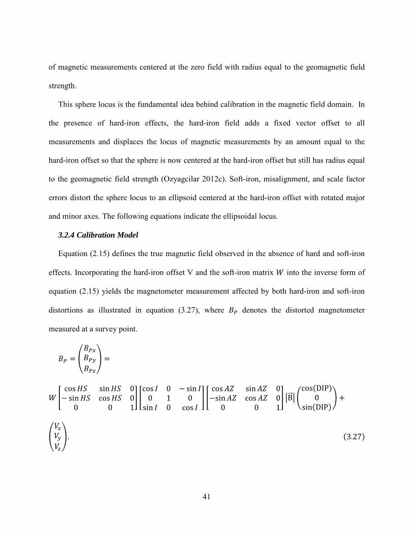
The sensor readings of the local gravity and the corrupted local magnetic field components at
each survey station are measured along instrument-fixed coordinate frame and entered to the
error compensation model of the MSA or the hard- and soft-iron to solve for magnetic
disturbances Three components of the geomagnetic vector including the field strength the
declination angle and the dip angle at the location of drilling operation are acquired from an
external reference source such as IGRF model freely over the internet in order to add to the
above models Eventually the corrected magnetic field measurements are used in the well-
known azimuth expressions such as (219) and (220) to derive the corrected borehole azimuth
along the borehole path at the point at which the readings were taken The BHA position is then
computed by assuming certain trajectory between the surveying stations
31 MSA Correction Model
The MSA algorithm assumes common error components to all surveys in a group and solves
for these unknown biases by minimizing the variance of the computed magnetic field values
about the central (reference) value of the local field to obtain calibration values The central
values may be either independent constants obtained from an external source of the local
magnetic field or the mean value of the computed local magnetic field (Brooks et al 1998)
Where the common cross-axial and axial magnetic bias components ∆119861119909 ∆119861119910 and ∆119861119911 are
affecting the measured components 119861119909119898(120003) 119861119910119898(120003) and 119861119911119898(120003) at 120003P
th survey station in the (X
Y Z) frame respectively the corrected values are calculated by
119861119909119862119900119903119903(120003) = 119861119909119898(120003) minus ∆119861119909 (31)
32
119861119910119862119900119903119903(120003) = 119861119910119898(120003) minus ∆119861119910 (32)
119861119911119862119900119903119903(120003) = 119861119911119898(120003) minus ∆119861119911 (33)
The vertical and horizontal components of the true geomagnetic field acquired from an
external reference source (such as IGRF) at the location of the borehole are denoted as
119861119881(119903119890119891) 119861ℎ(119903119890119891) respectively Moreover the vertical component of the local magnetic field at the
120003P
th survey station denoted as 119861119881(120003) is computed by the vector dot product
119861 g119861119881 = (34)
g
By substituting Equations (27) (214) for the 120003P
th survey station the computed value of local
field is obtained from
119861119909119862119900119903119903(120003) 119866119909(120003) + 119861119910119862119900119903119903(119899) 119866119910(120003) + 119861119911119862119900119903119903(120003) 119866119911(120003)119861119881(120003) = (35) 2 05
119866119909(120003)2 + 119866119910(120003)
2 + 119866119911(120003)
2 05119861ℎ(120003) = 119861119909119862119900119903119903(120003)
2 + 119861119910119862119900119903119903(120003)2 + 119861119911119862119900119903119903(120003)
2 minus 119861119881(120003) (36)
Values of the computed magnetic field 119861119881(120003) and 119861ℎ(120003) for a survey group at a range of 120003 =
1 hellip N will typically exhibit some scatter with respect to the reference value of 119861119881(119903119890119891) and
119861ℎ(119903119890119891) therefore reflecting the varying direction of drillstring magnetization error (Brooks
1997) This scatter formulated as variance (distance) among computed magnetic field values and
the reference local field value over N surveys is expressed as (Brooks et al 1998)
119873 2 21119985 =(119873minus1)
119861ℎ(120003) minus 119861ℎ(119903119890119891) + 119861119881(120003)minus119861119881(119903119890119891) (37) 120003=1
The unknown biases are solved for by minimizing this scatter through minimizing the
variance 119985 expressed in equation (37) This can be accomplished by differentiating equation
(37) with respect to the small unknown biases and setting the results to zero
33
The differentiations are nonlinear with respect to unknown biases An approximate solution
can therefore be found by linearizing the differentiations and solving for the unknown biases by
an iterative technique such as Newtonrsquos method in which successive approximations to the
unknown biases are found The updated bias estimates are replaced with previous estimates to
refine the values of the computed magnetic field for the next iteration The computation process
has been investigated in detail in US pat Nos 5623407 to Brooks and are also explained as
following
MSA Computation
From equation (37) where the small perturbations of ∆119861119909 ∆119861119910 and ∆119861119911 can be denoted as
120576119909 120576119910 and 120576119911 differentiations give
120597120597119985 119865 120576119909 120576119910 120576119911 = =
120597120597120576119909
119873
120597120597119861ℎ(120003) 120597120597119861ℎ(119903119890119891)= 119861ℎ(120003) minus 119861ℎ(119903119890119891) minus 120597120597120576119909 120597120597120576119909
120003=1
120597120597119861119881(120003) 120597120597119861119881(119903119890119891)+ 119861119881(120003) minus 119861119881(119903119890119891) minus = 0 (38) 120597120597120576119909 120597120597120576119909
120597120597119985 119866 120576119909 120576119910 120576119911 = =
120597120597120576119910
119873
120597120597119861ℎ(120003) 120597120597119861ℎ(119903119890119891)= 119861ℎ(120003) minus 119861ℎ(119903119890119891) minus 120597120597120576119910 120597120597120576119910
120003=1
120597120597119861119881(120003) 120597120597119861119881(119903119890119891)minus = 0 (39) + 119861119881(120003) minus 119861119881(119903119890119891) 120597120597120576119910 120597120597120576119910
34
120597120597119985 119867 120576119909 120576119910 120576119911 = =
120597120597120576119911
119873
120597120597119861ℎ(120003) 120597120597119861ℎ(119903119890119891)= 119861ℎ(120003) minus 119861ℎ(119903119890119891) minus 120597120597120576119911 120597120597120576119911
120003=1
120597120597119861119881(120003) 120597120597119861119881(119903119890119891)minus = 0 (310) + 119861119881(120003) minus 119861119881(119903119890119891) 120597120597120576119911 120597120597120576119911
The differentiations 119865 119866 and 119867 are nonlinear with respect to 120576119909 120576119910 and 120576119911 An approximate
solution can therefore be found by linearizing equations (38) through (310) by an iterative
technique such as Newtonrsquos method The linearized form of 119865 119866 and 119867 denoted as 119891 119892 and ℎ
are
119891 = 1198861 (120576119909 minus 120576119909 prime) + 1198871 120576119910 minus 120576119910
prime + 1198881 (120576119911 minus 120576119911 prime) + 119865 120576119909 prime 120576119910
prime 120576119911 prime = 0 (311)
119892 = 1198862 (120576119909 minus 120576119909 prime) + 1198872 120576119910 minus 120576119910
prime + 1198882 (120576119911 minus 120576119911 prime) + 119866 120576119909 prime 120576119910
prime 120576119911 prime = 0 (312)
ℎ = 1198863 (120576119909 minus 120576119909 prime) + 1198873 120576119910 minus 120576119910
prime + 1198883 (120576119911 minus 120576119911 prime) + 119867 120576119909 prime 120576119910
prime 120576119911 prime = 0 (313)
where
120597120597119865 120576119909 prime 120576119910
prime 120576119911 prime 120597120597119865 120576119909 prime 120576119910
prime 120576119911 prime 120597120597119865 120576119909 prime 120576119910
prime 120576119911 prime1198861 = 1198871 = 1198881 = (314) 120597120597120576119909 120597120597120576119910 120597120597120576119911
120597120597119866 120576119909 prime 120576119910
prime 120576119911 prime 120597120597119866 120576119909 prime 120576119910
prime 120576119911 prime 120597120597119866 120576119909 prime 120576119910
prime 120576119911 prime 1198862 = 1198872 = 1198882 = (315)
120597120597120576119909 120597120597120576119910 120597120597120576119911
120597120597119867 120576119909 prime 120576119910
prime 120576119911 prime 120597120597119867 120576119909 prime 120576119910
prime 120576119911 prime 120597120597119867 120576119909 prime 120576119910
prime 120576119911 prime 1198863 = 1198873 = 1198883 = (316)
120597120597120576119909 120597120597120576119910 120597120597120576119911
The primed error terms 120576119909 prime 120576119910
prime and 120576119911 prime represent the previous estimates of these values The
linearized equations (311) through (313) can be solved for the unknowns 120576119909 120576119910 and 120576119911 by
35
iterative technique of Newtonrsquos method in which successive approximations to 120576119909 120576119910 and 120576119911 are
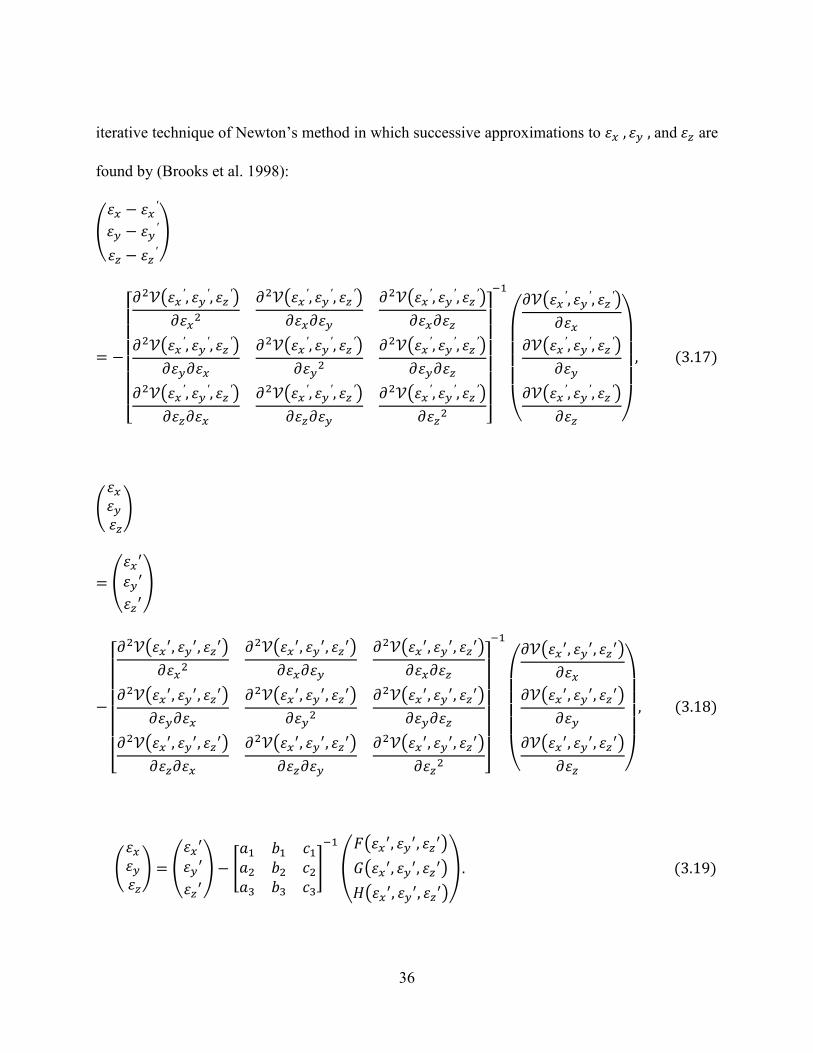
found by (Brooks et al 1998)
120576119909 minus 120576119909 prime
120576119910 minus 120576119910 prime
120576119911 minus 120576119911 prime
minus1
⎡1205971205972119985 120576119909
prime 120576119910 prime 120576119911 prime 1205971205972119985 120576119909
prime 120576119910 prime 120576119911 prime 1205971205972119985 120576119909
prime 120576119910 prime 120576119911 prime 120597120597119985 120576119909
prime 120576119910 prime 120576119911 prime⎤
⎢ 1205971205971205761199092 120597120597120576119909120597120597120576119910 120597120597120576119909120597120597120576119911 ⎥ ⎛ 120597120597120576119909 ⎞⎢1205971205972119985 120576119909
prime 120576119910 prime 120576119911 prime 1205971205972119985 120576119909
prime 120576119910 prime 120576119911 prime 1205971205972119985 120576119909
prime 120576119910 prime 120576119911 prime ⎥ ⎜120597120597119985 120576119909
prime 120576119910 prime 120576119911 prime ⎟
= minus ⎢ ⎥ ⎜ ⎟ (317) ⎢ 120597120597120576119910120597120597120576119909 1205971205971205761199102 120597120597120576119910120597120597120576119911 ⎥ ⎜ 120597120597120576119910 ⎟
⎜ ⎟⎢1205971205972119985 120576119909 prime 120576119910
prime 120576119911 prime 1205971205972119985 120576119909 prime 120576119910
prime 120576119911 prime 1205971205972119985 120576119909 prime 120576119910
prime 120576119911 prime ⎥ 120597120597119985 120576119909 prime 120576119910
prime 120576119911 prime⎢ ⎥ ⎣ 120597120597120576119911120597120597120576119909 120597120597120576119911120597120597120576119910 1205971205971205761199112 ⎦ ⎝ 120597120597120576119911 ⎠
120576119909 120576119910120576119911
prime120576119909prime = 120576119910 prime120576119911
minus1 prime prime prime prime prime prime prime ⎡1205971205972119985 120576119909 120576119910 120576119911prime 1205971205972119985 120576119909 120576119910 120576119911prime 1205971205972119985 120576119909 120576119910 120576119911prime 120597120597119985 120576119909prime 120576119910 120576119911prime⎤ ⎢ 1205971205971205761199092 120597120597120576119909120597120597120576119910 120597120597120576119909120597120597120576119911 ⎥ ⎛ 120597120597120576119909 ⎞⎢ prime prime prime prime prime prime ⎥ prime prime1205971205972119985 120576119909 120576119910 120576119911prime 1205971205972119985 120576119909 120576119910 120576119911prime 1205971205972119985 120576119909 120576119910 120576119911prime ⎜120597120597119985 120576119909 120576119910 120576119911prime ⎟ minus ⎢ ⎥ ⎜ ⎟ (318) ⎢ 120597120597120576119910120597120597120576119909 1205971205971205761199102 120597120597120576119910120597120597120576119911 ⎥ ⎜ 120597120597120576119910 ⎟
⎜ ⎟⎢ prime prime prime prime prime prime ⎥ prime prime1205971205972119985 120576119909 120576119910 120576119911prime 1205971205972119985 120576119909 120576119910 120576119911prime 1205971205972119985 120576119909 120576119910 120576119911prime 120597120597119985 120576119909 120576119910 120576119911prime⎢ ⎥ ⎣ 120597120597120576119911120597120597120576119909 120597120597120576119911120597120597120576119910 1205971205971205761199112 ⎦ ⎝ 120597120597120576119911 ⎠
prime prime 120576119909 120576119909prime 1198861 1198871 1198881 minus1 119865 120576119909 120576119910 120576119911prime
prime prime prime120576119910 = 120576119910 minus 1198862 1198872 1198882 119866 120576119909 120576119910 120576119911prime (319) prime120576119911 120576119911 1198863 1198873 1198883 119867 120576119909prime 120576119910prime 120576119911prime
36
The updated bias estimates of 120576119909 120576119910 and 120576119911 obtained from equation (319) is replaced with
previous estimates of 120576119909 120576119910 and 120576119911 in equations (31) through (33) to refine the values of
119861119909119862119900119903119903(120003) 119861119910119862119900119903119903(120003) and 119861119911119862119900119903119903(120003) for the next iteration
A suitable convergence criterion is used to determine whether further iterations are needed
The stopping criterion for the iteration can be defined as the change between successive values
of 120576119909 120576119910 and 120576119911 falling below a predefined minimum limit or a specified number of iterations
having been performed (Brooks et al 1998)
The derivatives 1198861 through 1198883 can be obtained by use of the chain rule In the case where the
central values are independent constants obtained from an external source of the local magnetic
field 1198861 is derived by
119873
1205971205972119861ℎ(120003)1198861 = 119873 minus 119861ℎ(119903119890119891) (320) 1205971205971205761199092
120003=1
In the case where the central values are the mean values of the computed local magnetic field
which are not constant the coefficient 1198861 is derived more complicated as
119873119873 ⎡ 1205971205972119861ℎ(120003) ⎤ ⎢ 2 1 2 1 ⎛ 1205971205971205761199092 ⎞⎥120597120597119861ℎ(120003) 120597120597119861119881(120003) 120003=1 1198861 = 119873 minus ⎢ ⎜119861ℎ(120003) ⎟⎥ (321) ⎢ 120597120597120576119909 119873
+ 120597120597120576119909 119873
+ ⎜ 119873 ⎟⎥
⎢ ⎥120003=1 ⎣ ⎝ ⎠⎦
where
2⎡ 2 ⎤
1205971205972119861ℎ(120003) 1 119866119909(120003) 119861119909119862119900119903119903(120003) + 119861119881(120003)
minus119866|g119909|
(120003)
⎢ ⎥⎛ ⎞= ⎢1 minus | minus ⎥ (322) 1205971205971205761199092 119861ℎ(120003) |g minus119861ℎ(120003)⎢ ⎥
⎣ ⎝ ⎠ ⎦
37
120597120597119861ℎ(120003) 119861119909119862119900119903119903(120003) + 119861119881(120003)
minus119866|g119909|
(120003)
= (323) 120597120597120576119909 minus119861ℎ(120003)
120597120597119861119881(120003) minus119866119909(120003)= (324) 120597120597120576119909 |g|
Similar calculations can derive the remaining coefficients 1198871 through 1198883 Upon completion of
the iteration the compensated magnetic field vectors which are now more closely grouped than
the primary scatter are used in well-known azimuth expressions such as (219) and (220) to
derive the corrected borehole azimuth (Brooks 1997)
32 Hard-Iron and Soft-Iron Magnetic Interference Calibration
A magnetometer senses the geomagnetic field plus magnetic field interference generated by
ferromagnetic materials on the probe By convention this magnetic field interference is divided
into static (fixed) hard-iron offset and induced soft-iron distortions
A mathematical calibration algorithm was developed by Ozyagcilar (2012) which is available
via Freescale application document number of AN4246 at httpwwwfreescalecom This
algorithm calibrates the magnetometers in the magnetic field domain to estimate magnetometer
output errors and remove the hard-iron and soft-iron interference from the magnetometer
readings taken under different probe orientations allowing the geomagnetic field components to
be measured accurately (Ozyagcilar 2012c) The calibration problem is solved through the
transformation of the locus of magnetometer measurements from the surface of an ellipsoid
displaced from the origin to the surface of a sphere located at the origin
321 Static Hard-Iron Interference Coefficients
Since the magnetometer and all components on the probe are in fixed positions with respect to
each other and they rotate together the hard-iron effect is independent of the probe orientation
38
and is therefore modeled as a fixed additive magnetic vector which rotates with the probe Since
any zero field offset in the magnetometer factory calibration is also independent of the probe
orientation it simply appears as a fixed additive vector to the hard-iron component and is
calibrated and removed at the same time Both additive vectors are combined as a hard-iron
vector V with components of V119909 V119910 and V119911 adding to the true magnetometer sensor output
(Ozyagcilar 2012a) Therefore the standard hard-iron estimation algorithms compute the sum of
any intrinsic zero fields offset within the magnetometer sensor itself plus permanent magnetic
fields within the probe generated by magnetized ferromagnetic materials (Ozyagcilar 2012a)
322 Soft-Iron Interference Coefficients
Soft-iron effects are more complex to model than hard-iron effects since the induced soft-iron
magnetic field depends on the orientation of the probe relative to the geomagnetic field
(Ozyagcilar 2012c) The assumption is that the induced soft-iron field is linearly related to the
inducing local geomagnetic field measured in the rotated probe (Ozyagcilar 2012b) This linear
relationship is mathematically expressed by the 3 times 3 matrix 119882119878119900119891119905 The components of 119882119878119900119891119905
are the constants of proportionality between the inducing local magnetic field and the induced
soft-iron field For example the component in the first raw of the second column of 119882119878119900119891119905
represents the effective coefficient relating the induced field generated in the x-direction in
response to an inducing field in the y-direction Thus 119882119878119900119891119905 can be a full matrix
The magnetometer is normally calibrated by the company to have approximately equal gain in
all three axes Any remaining differences in the gain of each axis can be modeled by a diagonal
3 times 3 gain matrix 119882119866119886119894119899 which is also referred to as scale factor error Another 3 times 3 matrix
119882119873119900119899119874119903119905ℎ119900119892 referred to as misalignment error is used to model
39
(i) The rotation of magnetometer relative to the instrument-fixed coordinate system (X Y
Z)
(ii) The lack of perfect orthogonality between sensor axes (Ozyagcilar 2012b)
Since the misalignment between the two axes is normally very small (but not negligible)
119882119873119900119899119874119903119905ℎ119900119892 can be modelled as the following symmetric matrix (Gebre-Egziabher et al 2001)
1 minus120576119911 120576119910
119882119873119900119899119874119903119905ℎ119900119892 = 120576119911 1 minus120576119909 (325) minus120576119910 120576119909 1
The three independent parameters 120576119909 120576119910 and 120576119911defining the matrix 119882119873119900119899119874119903119905ℎ119900119892represent
small rotations about the body axes of the vehicle that will bring the platform axes into perfect
alignment with the body axes The linear soft-iron model is derived from the product of these
three independent matrices which results in nine independent elements of a single 3 by 3 soft-
iron matrix 119882 defined as
119882 = 119882119873119900119899119874119903119905ℎ119900119892 119882119866119886119894119899 119882119878119900119891119905 (326)
The process of calibrating a triad of magnetometers involves estimating the hard-iron vector
V and the soft-iron matrix W defined above
323 Relating the Locus of Magnetometer Measurements to Calibration Coefficients
In complete absence of hard-iron and soft-iron interference a magnetometer will measure the
uncorrupted geomagnetic field and thus the vector magnitude of the measured field will equal the
magnitude of the geomagnetic field As a result at different probe orientations the measured
magnetic field components along the instrument-fixed coordinate system (X Y Z) will be
different but the vector magnitude will not change Therefore the locus of the magnetometer
measurements under arbitrary orientation changes will lie on the surface of a sphere in the space
40
of magnetic measurements centered at the zero field with radius equal to the geomagnetic field
strength
This sphere locus is the fundamental idea behind calibration in the magnetic field domain In
the presence of hard-iron effects the hard-iron field adds a fixed vector offset to all
measurements and displaces the locus of magnetic measurements by an amount equal to the
hard-iron offset so that the sphere is now centered at the hard-iron offset but still has radius equal
to the geomagnetic field strength (Ozyagcilar 2012c) Soft-iron misalignment and scale factor
errors distort the sphere locus to an ellipsoid centered at the hard-iron offset with rotated major
and minor axes The following equations indicate the ellipsoidal locus
324 Calibration Model
Equation (215) defines the true magnetic field observed in the absence of hard and soft-iron
effects Incorporating the hard-iron offset V and the soft-iron matrix 119882 into the inverse form of
equation (215) yields the magnetometer measurement affected by both hard-iron and soft-iron
distortions as illustrated in equation (327) where 119861119875 denotes the distorted magnetometer
measured at a survey point
119861119875119909119861119875 = 119861119875119910 =
119861119875119911
119882 cos 119867119878 minus sin 119867119878
sin 119867119878 cos 119867119878
0 0
cos 119868 0
0 1 minus sin 119868
0 cos 119860119885 minussin 119860119885
sin 119860119885 cos 119860119885
0 0 B
cos(DIP)0 +
0 0 1 sin 119868 0 cos 119868 0 0 1 sin(DIP)
119881119909119881119910
119881119911 (327)
41
In a strong hard and soft-iron environment the locus of magnetometer measurements under
arbitrary rotation of the probe lie on a surface which can be derived as (Ozyagcilar 2012b)
119882minus1 119861119901 minus V119879119882minus1 119861119901 minus V = 119861119901 minus V
119879119882minus1119879119882minus1 119861119901 minus V = B2 (328)
substituting from equation (327) and denoting
cos 119867119878 sin 119867119878 0 cos 119868 0 minus sin 119868 cos 119860119885 sin 119860119885 0 minus sin 119867119878
0 cos 119867119878
0 0 1
0 sin 119868
1 0
0 cos 119868
minussin 119860119885 0
cos 119860119885 0
0 1
= Γ (329)
results in
119882minus1 119861119901 minus V = Γ B cos(DIP)
0 sin(DIP)
(330)
Therefore it is proved that
119882minus1 119861119901 minus V119879119882minus1 119861119901 minus V = Γ B
cos(DIP)0
sin(DIP)
119879
Γ B cos(DIP)
0 sin(DIP)
= B2 (331)
In general the locus of the vector 119861119901 lying on the surface of an ellipsoid with center
coordinate of the vector V is expressed as
119861119901 minus V119879
A 119861119901 minus V = 119888119900119899119904119905 (332)
Where matrix A must be symmetric Equation (331) and (332) are similar since it can be
easily proved that the matrix 119882minus1119879119882minus1 is symmetric as 119860119879 = [119882minus1119879119882minus1]119879 =
119882minus1119879119882minus1 = A Thus in a strong hard and soft-iron environment the locus of raw
magnetometer measurements forms the surface of an ellipsoid defined by
119861119901 minus V119879119882minus1119879119882minus1 119861119901 minus V = B2 (333)
42
The ellipsoid is centered at the hard-iron offset V Its size is defined by the geomagnetic field
strength B and its shape is determined by the matrix 119882minus1119879119882minus1 which is transposed square of
the inverse soft-iron matrix 119882minus1
In the absence of soft-iron and misalignment errors the diagonal 3 times 3 scale factor
matrix 119882119866119886119894119899 distorts the sphere locus along preferred axes with differing gains along each axis
The measurement locus then becomes an ellipsoid centered at the hard-iron offset with the
major and minor axesrsquo magnitudes determined by the scale factor errors 119904119891119909 119904119891119910 and 119904119891119911 along
the instrument-fixed coordinate frame This can be expressed mathematically as follows
(1 + 119904119891119909) 0 0 119882119866119886119894119899 = 0 (1 + 119904119891119910) 0 (334)
0 0 (1 + 119904119891119911)
1⎡ 0 0 ⎤1 + 119904119891119909 ⎢ ⎥
minus1 ⎢ 1 ⎥119882119866119886119894119899 = ⎢ 0 0 ⎥ (335) 1 + 119904119891119910 ⎢ ⎥1⎢ ⎥0 0⎣ 1 + 119904119891119911⎦
119861119901 minus V119879
119882119866119886119894119899minus1119879 119882119866119886119894119899minus1 119861119901 minus V = 1198612 (336)
2⎡ 0 0 ⎤ ⎢ 1 +
1 119904119891119909
⎥
2⎢ 1 ⎥119861119901 minus V
119879
⎢ 0 0 ⎥ 119861119901 minus V = 1198612 (337) ⎢ 1 + 119904119891119910
⎥2
⎢ ⎥0 0 ⎣ 1 +
1 119904119891119911
⎦
Mathematically the locus of measurements is described by the following equation
2 2 2 119861119875119909 minus 119881119909 119861119875119910 minus 119881119910 + 119861119875119911 minus 119881119911+ = 1198612 (338)
1 + 119904119891119909
1 + 119904119891119910
1 + 119904119891119911
43
Soft-iron and misalignment errors will modify the error-free sphere locus into an ellipsoid but
also rotate the major and minor axes of the ellipsoid Thus the ellipsoid does not need to be
aligned with the axes of the magnetometer and the ellipsoid can be non-spherical
Magnetometer measurements subject to both hard-iron and soft-iron distortions lying on the
surface of an ellipsoid can be modeled by nine ellipsoid parameters comprising the three
parameters which model the hard-iron offset and six parameters which model the soft-iron
matrix The calibration algorithm that will be developed is nothing more than a parameter
estimation problem The algorithm is an attempt to fit the best ellipsoid in least-squares sense to
the measured magnetometer data The calibration algorithm consists of mathematically removing
hard-iron and soft-iron interference from the magnetometer readings by determining the
parameters of an ellipsoid that best fits the data collected from a magnetometer triad (Gebre-
Egziabher et al 2001)
After the nine model parameters are known the magnetometer measurements are transformed
from the surface of ellipsoid to the surface of a sphere centered at the origin This transformation
removes the hard-iron and soft- iron interference and then the calibrated measurements are used
to compute an accurate azimuth (Ozyagcilar 2012b)
325 Symmetric Constrait
The linear ellipsoid model of 119861119901 minus V119879119882minus1119879119882minus1 119861119901 minus V = B2 is solved for the
transposed square of the inverse soft-iron matrix 119882minus1119879119882minus1and the hard-iron vector V by
optimum fitting of the ellipsoid to the measured data points The ellipsoid fit provides the matrix
119882minus1119879119882minus1 whereas the calculation of the calibrated magnetic field measurement 119861119875119862119886119897
according to equation (339) requires the inverse soft-iron matrix 119882minus1
44
119861119875119909 minus 119881119909
119861119875119862119886119897 = 119882minus1 119861119875119910 minus 119881119910 (339) 119861119875119911 minus 119881119911
Although it is trivial to compute the ellipsoid fit matrix 119882minus1119879119882minus1 from the inverse soft-
iron matrix 119882minus1 there is no unique solution to the inverse problem of computing 119882minus1 from the
matrix 119882minus1119879119882minus1 The simplest solution is to impose a symmetric constraint onto the inverse
soft-iron matrix 119882minus1 As proved in equation (332) the matrix 119882minus1119879119882minus1 is symmetric with
only six independent coefficients while the soft-iron matrix 119882 has nine independent elements
This means that three degrees of freedom are lost Physically it can be understood as a result of
the loss of angle information in the ellipsoidal locus of the measurements constructed in the
mathematical model which is a function of the magnetometer measurements only (Ozyagcilar
2012b)
To solve this problem a constraint is imposed that the inverse soft-iron matrix 119882minus1 also be
symmetric with six degrees of freedom The reading 119861119901 is calibrated by an estimated hard-iron
offset 119881119862119886119897 and an estimated soft-iron matrix 119882119862119886119897 then the resulting corrected magnetic field
measurement 119861119875119862119886119897 is given by
cos(DIP)119861119875119862119886119897 = 119882C119886119897minus1 119861119901 minus 119881119862119886119897 = 119882119862119886119897minus1 119882 Γ B 0 + 119881 minus 119881119862119886119897 (340)
sin(DIP)
If the calibration algorithm correctly estimates the hard and soft-iron coefficients then the
corrected locus of reading lie on the surface of a sphere centered at the origin Therefore in
equation (340) it is necessary that 119882119862119886119897minus1119882 = I and 119881119862119886119897 = 119881 thus resulting in
) = B2 (341) (119861119875119862119886119897)119879(119861119875119862119886119897
45
Mathematically an arbitrary rotation can be incorporated in the estimated inverse soft-iron
minus1 matrix 119882119862119886119897 as 119882119862119886119897minus1119882 = 119877(120589) where 119877(120589) is the arbitrary rotation matrix by angle 120589
Considering that the transpose of any rotation matrix is identical to rotation by the inverse angle
leads to 119877(120589)119879 = 119877(minus120589) Substituting 119881119862119886119897 = 119881 in equation (340) yields
cos(DIP)119861119875119862119886119897 = 119882119862119886119897minus1 119861119901 minus 119881119862119886119897 = 119882119862119886119897minus1 119882 Γ B 0 (342)
sin(DIP)
cos(DIP) 119879 cos(DIP)) = 119882119862119886119897minus1 119882 Γ B 0 119882119862119886119897minus1 119882 Γ B 0 (343) (119861119875119862119886119897)
119879(119861119875119862119886119897 sin(DIP) sin(DIP)
then substituting 119882119862119886119897minus1 119882 = 119877(120589) yields
cos(DIP) 119879 cos(DIP)) = 119877(120589) Γ B 0 119877(120589) Γ B 0 = B2 (344) (119861119875119862119886119897)
119879(119861119875119862119886119897 sin(DIP) sin(DIP)
and substituting 119877(120589)119879 119877(120589) = 119877(minus120589) 119877(120589) = 119868 results in
cos(DIP) 119879 cos(DIP)) = B 0 Γ119879 119877(120589)119879 119877(120589) Γ B 0 = B2 (345) (119861119875119862119886119897)
119879(119861119875119862119886119897 sin(DIP) sin(DIP)
It was proved that by incorporating the spurious rotation matrix 119877(120589) the corrected locus of
measurements still lies on the surface of a sphere with radius B centered at the origin (Ozyagcilar
2012b) The reason is that a sphere is still a sphere under arbitrary rotation If the constraint is
applied that the inverse soft-iron matrix 119882minus1 is symmetric then it is impossible for any spurious
rotation matrix to be incorporated in the calibration process since any rotation matrix must be
anti-symmetric
A further advantage of a symmetric inverse soft-iron matrix 119882minus1 is the relationship between
the eigenvectors and eigenvalues of matrix 119882minus1119879119882minus1 and matrix 119882minus1 It can be proved that
46
if 119882minus1 is symmetric as 119882minus1119879 = 119882minus1 then the eigenvectors of matrix 119882minus1119879119882minus1 are
identical to the eigenvectors of matrix 119882minus1 and the eigenvalues of matrix 119882minus1119879119882minus1 are the
square of the eigenvalues of matrix 119882minus1 Eigenvectors 119883119894 and eigenvalues 119890119894 of 119882minus1 are
defined by 119882minus1 119883119894 = 119890119894 119883119894 Therefore
119882minus1119879119882minus1 119883119894 = 119882minus1119879119890119894 119883119894 = 119890119894119882minus1119883119894 = 1198901198942119883119894 (346)
Since the eigenvectors of the ellipsoid fit matrix 119882minus1119879119882minus1 represent the principal axes of
magnetometer measurement ellipsoidal locus then constraining the inverse soft iron matrix 119882minus1
to be symmetric shrinks the ellipsoid into a sphere along the principal axes of the ellipsoid
without applying any additional spurious rotation (Ozyagcilar 2012b)
The symmetric inverse soft-iron matrix 119882minus1 can be computed from the square root of the
ellipsoid fit matrix 119882minus1119879119882minus1 as following
119882minus1119879119882minus1 = 119882minus1119882minus1 119882minus1 = [ 119882minus1119879119882minus1]12 (347)
This is not always a reasonable assumption and it can be accounted for the residuals in post
process Furthermore examination of experimental data indicated that the careful installation of
magnetometersrsquo axes aligned with the body axes results in an ellipsoidal locus having major and
minor axes aligned with the body axes
326 Least-Squares Estimation
The calibration algorithm develops an iterated least-squares estimator to fit the ellipsoid
119886 119887 119888 parameters to the measured magnetic field data Substituting 119882minus1119879119882minus1 = 119887 119890 119891 in to
119888 119891 119868
Equation (333) results in
47
119886 119887 119888 119861119875119909 minus 119881119909
B2 = (119861119875119909 minus 119881119909 119861119875119910 minus 119881119910 119861119875119911 minus 119881119911) 119887 119890 119891 119861119875119910 minus 119881119910 (348) 119888 119891 119868 119861119875119911 minus 119881119911
|119861| = 119886(119861119875119909 minus 119881119909)2 + 119890 119861119875119910 minus 119881119910
2 + 119868(119861119875119911 minus 119881119911)2 + 2119887(119861119875119909 minus 119881119909) 119861119875119910 minus 119881119910 +
(349) +2119888(119861119875119909 minus 119881119909)(119861119875119911 minus 119881119911) + 2119891 119861119875119910 minus 119881119910 (119861119875119911 minus 119881119911)
The equations of the estimator can be obtained by linearizing Equation (349) The estimator
has perturbations of the ellipsoid parameters comprising three parameters of hard-iron offset and
six components of the soft-iron matrix (Gebre-Egziabher et al 2001) Thus given an initial
guess of the unknown parameters the estimated perturbations are sequentially added to the initial
guess and the procedure is repeated until convergence is achieved (Gebre-Egziabher et al 2001)
To linearize Equation (349) the perturbation of |119861| is written as 120575119861 given by
120597120597119861 120575a +
120597120597119861 120575c +
120597120597119861
120597120597b 120575b +
120597120597119861120575119861 = 120575119881119909 +
120597120597119861 120575119881119910 +
120597120597119861 120575119881119911 +
120597120597119861 120575e
120597120597119881119909 120597120597119881119910 120597120597119881119911 120597120597a 120597120597c 120597120597e
+ 120597120597119861
120597120597f 120575f +
120597120597119861
120597120597I 120575I (350)
where
120597120597119861 minus2119886 (119861119875119909 minus 119881119909) minus 2b 119861119875119910 minus 119881119910 minus 2c (119861119875119911 minus 119881119911) = (351)
120597120597119881119909 2119861
120597120597119861 minus2119890 119861119875119910 minus 119881119910 minus 2b (119861119875119909 minus 119881119909) minus 2f (119861119875119911 minus 119881119911) = (352)
120597120597119881119910 2119861
120597120597119861 minus2119868 (119861119875119911 minus 119881119911) minus 2c (119861119875119909 minus 119881119909) minus 2f (119861119875119910 minus 119881119910) = (353)
120597120597119881119911 2119861
120597120597119861 (119861119875119909 minus 119881119909)2
= (354) 120597120597a 2119861
120597120597119861 2(119861119875119909 minus 119881119909) 119861119875119910 minus 119881119910 (355)
120597120597b =
2119861
48
120597120597119861 2(119861119875119909 minus 119881119909)(119861119875119911 minus 119881119911) = (356)
120597120597c 2119861
120597120597119861 (119861119875119910 minus 119881119910)2
= (357) 120597120597e 2119861
120597120597119861 2 119861119875119910 minus 119881119910 (119861119875119911 minus 119881119911) (358)
120597120597f =
2119861
120597120597119861 (119861119875119911 minus 119881119911)2
(359) 120597120597I
=2119861
The given or known inputs to the calibration algorithm are the measured magnetometer
outputs 119861119875119909 119861119875119910 and 119861119875119911 and the magnitude of geomagnetic field vector in the geographic
area where the calibration is being performed Note that the 119861119875119909 119861119875119910 and 119861119875119911 values have been
taken in N positions even though for the sake of simplicity the explicit notation (index) has
been dropped in the above equations In matrix notation (350) can be expressed as
⎡ 1205751198611 ⎤1205751198612⎢ ⎥⋮ =⎢ ⎥ ⎢120575119861119873minus1⎥ ⎣ 120575119861119873 ⎦
120597120597119861 120597120597119861 120597120597119861 120597120597119861 120597120597119861 120597120597119861 120597120597119861 120597120597119861 120597120597119861⎡ ⎤ ⎢ 120597120597119881119909 120597120597119881119910 120597120597119881119911 1 120597120597a 1 120597120597b
120597120597c 1 120597120597e 120597120597f 1 120597120597I ⎥1 1 1 1 1
⎢ ⎥ 120597120597119861 120597120597119861 120597120597119861 120597120597119861 120597120597119861 120597120597119861 120597120597119861 120597120597119861 120597120597119861⎢ ⎥ ⎢ 120597120597119881119909 2 120597120597119881119910 2
120597120597119881119911 2 120597120597a 2 120597120597b 2 120597120597c 2 120597120597e 2 120597120597f 2 120597120597I 2 ⎥ ⎢ ⎥⋮ ⋱ ⋮⎢ ⎥ 120597120597119861 120597120597119861 120597120597119861 120597120597119861 120597120597119861 120597120597119861 120597120597119861 120597120597119861 120597120597119861⎢ ⎥ ⎢ 120597120597119881119909 119873minus1 120597120597119881119910 119873minus1
120597120597119881119911 119873minus1 120597120597a 119873minus1 120597120597b 119873minus1 120597120597c 119873minus1 120597120597e 119873minus1 120597120597f 119873minus1 120597120597I 119873minus1 ⎥ ⎢ ⎥ 120597120597119861 120597120597119861 120597120597119861 120597120597119861 120597120597119861 120597120597119861 120597120597119861 120597120597119861 120597120597119861⎢ ⎥ ⎣ 120597120597119881119909 119873 120597120597119881119910 119873
120597120597119881119911 119873 120597120597a 119873 120597120597b 119873 120597120597c 119873 120597120597e 119873 120597120597f 119873 120597120597I 119873 ⎦
49
⎡120575119881119909⎤120575119881119910⎢ ⎥120575119881119911⎢ ⎥ ⎢ 120575a ⎥
times ⎢ 120575b ⎥ (360) ⎢ 120575c ⎥ ⎢ 120575e ⎥ ⎢ 120575f ⎥ ⎣ 120575I ⎦
Equation (360) is in the form 120575119861 = the vector of unknowns is given by where 120575119883120577 120575119883
120575 = [120575119881119909 120575119881119910 120575119881119911 120575a 120575b 120575c 120575e 120575f 120575I]119879 (361)
The vector 120575119861 is the difference between the known geomagnetic field strength and its
magnitude computed from the magnetic measurements An estimate of the
successive perturbations of the ellipsoid parameters 119881119909 119881119910 119881119911 a b c 119890 119891 and I is obtained by
using the following iterative algorithm
Firstly select a non-zero initial guess for 119881119909 119881119910 119881119911 a b c 119890 119891 and I Secondly form
Equation (360) by the initial values Thirdly obtain a least square estimate for 120575 as follows
120575 = (120577119879120577)minus1120577119879 120575119861 (362)
Then update the unknown parameters by adding the 120575 perturbations to the current values of
parameters Finally return to the second step and repeat until convergence is achieved
Convergence is achieved when the estimate of 119881119909 119881119910 119881119911 a b c 119890 119891 and I do not change from
one iteration to the next By imposing the symmetric constraint stated in the last section the
inverse soft-iron matrix is obtained from the square root of the ellipsoid fit matrix The estimated
calibration parameters can then be used in Equation (339) to transform the measured raw data
lying on the ellipsoid into the corrected field measurements lying on the sphere centered at the
50
origin with radius equal to the geomagnetic field in the absence of hard and soft-iron
interference The computed azimuth using these corrected measurements will be highly accurate
327 Establishing Initial Conditions
The stability of the least squares solution is sensitive to the quality of the initial conditions
used to start the algorithm The closer the initial guesses are to the actual value of the nine
ellipsoidal parameters the more stable the solution becomes Since a judicious selection of
initial conditions enhances the performance of the calibration I will propose an algorithm to
establish the initial conditions for the iterative least-squares algorithm Equation (349) of the
ellipsoidal locus is non-linear in nature Nevertheless it can be treated as a desirable linear
system by breaking the parameter identification problem given by Equation (349) in to two steps
so as to estimate a good approximation of the initial values of the parameters The proposed two
step linear solution will now be explained
3271 Step 1 Hard-Iron Offset estimation
The hard-iron correction may be sufficient for the probe without strong soft-iron interference
because in most cases hard iron biases will have a much larger contribution to the total magnetic
corruption than soft iron distortions A simple solution can be permitted for the case where the
hard-iron offset dominates and soft-iron effects can be ignored Therefore the soft-iron matrix is
assumed to be an identity matrix and Equation (333) simplifies to sphere locus
119861119901 minus V119879119861119901 minus V = B2 (363)
This simplification results in determining just three calibration parameters modeling the hard-
iron offset plus the geomagnetic field strength B My applied Matlab code fits these four model
parameters of the above mentioned sphere to the series of magnetometer measurements taken
51
under different probe orientations while minimizing the fit error in a least-squares sense The
least-squares method minimizes the 2ndashnorm of the residual error by optimizing the calibration fit
and determines the sphere with radius equal to the geomagnetic field strength B centered at the
hard-iron offset V The number of measurements used to compute the calibration parameters
must be greater than or equal to four since there are four unknowns to be determined (Ozyagcilar
2012b) The detail of the computation of hard-iron offsets has been published by Ozyagcilar via
Freescale application notes number AN4246
The data is now centered at the origin but still highly distorted by soft-iron effects The
computed azimuth will not be accurate after applying hard-iron corrections only The calibrated
measurements can now be passed to the second step of the algorithm for calculating the soft-iron
interference
3272 Step 2 Solving Ellipsoid Fit Matrix by an Optimal Ellipsoid Fit to the Data
Corrected for Hard Iron Biases
The hard-iron vector V and the magnitude of geomagnetic field solved from step 1 are applied
in the step 2 solution Equation (333) is then written as
119886 119887 119888 119861119909119862119900119903_ℎ
B2 = (119861119909119862119900119903_ℎ 119861119910119862119900119903_ℎ 119861119911119862119900119903_ℎ) 119887 119890 119891 119861119910119862119900119903_ℎ (364) 119888 119891 119868 119861119911119862119900119903_ℎ
Where 119861119909119862119900119903_ℎ 119861119910119862119900119903_ℎ and 119861119911119862119900119903_ℎ are acquired by subtraction of the hard-iron vector V
(obtained from step 1) from 119861119909 119861119910 and 119861119911 measurements respectively
119886 119861119909119862119900119903_ℎ2 + 119890 119861119910119862119900119903_ℎ
2 + 119868 119861119911119862119900119903_ℎ2 + 2119887 119861119909119862119900119903_ℎ 119861119910119862119900119903_ℎ + 2119888 119861119909119862119900119903_ℎ 119861119911119862119900119903_ℎ
+ 2119891 119861119910119862119900119903_ℎ 119861119911119862119900119903_ℎ minus B2 = 119903 (365)
52
The least-squares method minimizes the 2ndashnorm of the residual error vector 119903 by fitting 6
components of the ellipsoid fit matrix 119882minus1119879119882minus1to the series of 119861119862119900119903_ℎ taken at N positions
expressed as follows
⎡ 119861119909119862119900119903ℎ21
119861119910119862119900119903ℎ21
119861119911119862119900119903ℎ21
119861119909119862119900119903ℎ times 119861119910119862119900119903ℎ 1
119861119909119862119900119903ℎ times 119861119911119862119900119903ℎ 1
⎢ 119861119909119862119900119903ℎ22
119861119910119862119900119903ℎ22
119861119911119862119900119903ℎ22
119861119909119862119900119903ℎ times 119861119910119862119900119903ℎ 2
119861119909119862119900119903ℎ times 119861119911119862119900119903ℎ 2⎢ ⋮ ⋱ ⋮⎢
⎢ 119861119909119862119900119903ℎ 119861119910119862119900119903ℎ
119861119911119862119900119903ℎ 119861119909119862119900119903ℎ
times 119861119910119862119900119903ℎ 119861119909119862119900119903ℎ
times 119861119911119862119900119903ℎ⎢ 2119873minus1
2119873minus1
2119873minus1 119873minus1 119873minus1
⎣ 119861119909119862119900119903ℎ2119873
119861119910119862119900119903ℎ2119873
119861119911119862119900119903ℎ2119873
119861119909119862119900119903ℎ times 119861119910119862119900119903ℎ 119873
119861119909119862119900119903ℎ times 119861119911119862119900119903ℎ 119873
(366)
where in Equation (366)
⎣ ⎢ ⎢ ⎢ ⎢ ⎢ ⎡ 119861119909119862119900119903ℎ
21
119861119909119862119900119903ℎ 22⋮
119861119909119862119900119903ℎ 2119873minus1
119861119909119862119900119903ℎ 2119873
119861119910119862119900119903ℎ 21
119861119910119862119900119903ℎ 22
119861119910119862119900119903ℎ 2119873minus1
119861119910119862119900119903ℎ 2119873
119861119911119862119900119903ℎ 21
119861119911119862119900119903ℎ 22
119861119911119862119900119903ℎ 2119873minus1
119861119911119862119900119903ℎ 2119873
119861119909119862119900119903ℎ times 119861119910119862119900119903ℎ 1
119861119909119862119900119903ℎ times 119861119910119862119900119903ℎ 2
⋱ 119861119909119862119900119903ℎ
times 119861119910119862119900119903ℎ 119873minus1
119861119909119862119900119903ℎ times 119861119910119862119900119903ℎ 119873
119861119909119862119900119903ℎ times 119861119911119862119900119903ℎ 1
119861119909119862119900119903ℎ times 119861119911119862119900119903ℎ 2
⋮ 119861119909119862119900119903ℎ
times 119861119911119862119900119903ℎ 119873minus1
119861119909119862119900119903ℎ times 119861119911119862119900119903ℎ 119873
53
⎤ is denoted as matrix A and ⎢
⎡BB
⋮22
⎥ is denoted as vector l The least-squares solution for the ⎢ ⎥ ⎢B2⎥ ⎣B2⎦
vector of unknowns is given by
119886⎡ 119890 ⎤ ⎢ 119868 ⎥ ⎢2119887⎥ = ( A119879A)minus1A119879119897 (367) ⎢ ⎥ ⎢2119888⎥ ⎣2119891⎦
Afterwards the inverse soft-iron matrix 119882minus1 can be computed from the square root of the
ellipsoid fit matrix 119882minus1119879119882minus1 This algorithm can compute initial values of hard-iron and
soft-iron distortions by magnetometer measurements in the complete absence of a-priori
information about the direction and strength of the geomagnetic field
33 Well path Design and Planning
Well path design and planning employs several methods of computation of well trajectory
parameters to create the well path Each method is able to provide pictorial views both in the
vertical and horizontal plane of the trajectory position of the drilling bit in the wellbore
Eventually it is been able to compute the position at each survey station and therefore predict the
length and direction from a survey station relative to the target position This helps to detect the
deviations with less ease and therefore initiate the necessary directional corrections or adjustment
in order to re-orient the drilling bit to the right course before and during the drilling operations
(Amorin and Broni-Bediako 2010) These computations are required to be done ahead of time
before drilling resumes and also during drilling operations to minimize risk and the uncertainty
surrounding hitting a predetermined target (Sawaryn and Thorogood 2003) Therefore as the
54
well is surveyed during the various stages of drilling and construction the position of the well
path is recorded and plotted as a course line or trajectory in software plots (Lowdon and Chia
2003)
The survey calculation methods of well trajectory available in the industry are the Tangential
Balanced Tangential Average Angle Mercury Radius of Curvature and the Minimum
Curvature methods The main difference in all these techniques is that one group uses straight
line approximations and the other assumes the wellbore is more of a curve and is approximated
with curved segments The Tangential Balanced Tangential Average Angle and Mercury are
applicable to a wellbore trajectory which follows a straight line course while the Radius of
Curvature is strictly applicable to a wellbore trajectory that follows a curved segment The
Minimum Curvature method is applicable to any trajectory path
Bourgoyne et al (1991) showed that the Tangential method which is a simplistic method
assuming straight-line segments with constant angles along the well trajectory shows
considerable error for the northing easting and elevation which makes it no longer preferred in
the industry The differences in results obtained using the Balanced Tangential Average Angle
Mercury Radius of Curvature and Minimum Curvature are very small hence any of the methods
could be used for calculating the well trajectory
Realistically well paths are curved as the wellbore trajectory is built up The method of
applying a minimum curvature to the well path takes into account the graduation of the angles in
three dimensions along the wellbore trajectory and hence is a better approximation Minimum
Curvature is the most widely preferred method in the oil industry since it is applicable to any
trajectory path and thus more emphasis would be placed on this rather than the other methods
(Amorin and Broni-Bediako 2010) All the Minimum Curvature methods assume that the hole is
55
a spherical arc with a minimum curvature or a maximum radius of curvature between stations
and the wellbore follows a smoothest possible circular arc between stations that is the two
adjacent survey points lie on a circular arc This arc is located in a plane whose orientation is
defined by known inclination and direction angles at the ends of the arc (Bourgoyne et al 1991)
The calculation process requires data input containing measured Depth inclination angles and
corrected Bearing (Azimuths) with their corresponding descriptive data of the station ID
Moreover spatial data of the reference station (initial or starting coordinates) and magnetic
declination are required The direction for the magnetic declination angle must be specified if
the magnetic declination is to westward the sign is negative otherwise it is positive Figure 3-1
shows the geometry of the Tangential method and Figure 3-2 shows the geometry of the
Minimum Curvature method
Figure 3-1 Representation of the geometry of the tangential method(Amorin and Broni-
Bediako 2010)
56
Figure 3-2 Representation of the geometry of the minimum curvature method
(Amorin and Broni-Bediako 2010)
The Minimum Curvature method effectively fits a spherical arc between points by calculating
the ldquodog-legrdquo (DL) curvature and scaling by a ratio factor (RF) The spatial coordinates of
easting northing and elevation can be computed by the Minimum Curvature method as follows
(Amorin and Broni-Bediako 2010)
∆119879119881119863 = ∆119872119863
(cos 1198681 + cos 1198682)(RF) (368) 2
∆119873119900119903119905ℎ = ∆119872119863
(sin 1198681 times cos 1198601198851 + sin 1198682 times cos 1198601198852)(RF) (369) 2
∆119864119886119904119905 = ∆119872119863
[(sin 1198681 times sin 1198601198851 +sin 1198682 times sin 1198601198852)](RF) (370) 2
DL = cosminus1 cos(1198682 minus 1198681) minus sin 1198681 times sin 1198682 times [1 minus cos(1198601198852 minus 1198601198851)] (371)
22
119877119865 = DL
times tan 119863119871
(372)
57
where
∆= Change in parameter MD = Measured depth TVD = True vertical depth
1198601198851 = Azimuth angle at upper survey point
1198601198852 = Azimuth angle at lower survey point
1198681 = Inclination angle at upper survey point
1198682 = Inclination angle at lower survey point
DL = ldquodog-legrdquo curvature
119877119865 = Ratio factor for minimum curvature
34 Summary
In the directional drilling operation the computing device on the surface is programmed in
accordance with the magnetic correction methods For this research I have developed my Matlab
program either in accordance with MSA or hard- and soft-iron algorithm The inputs to the
program include the x-axis y-axis and z-axis components of the local magnetic and
gravitational field at each survey station Furthermore an external estimate of the local
geomagnetic field at the location of the wellbore is added to the program inputs The magnetic
disturbances solved by the program are used to correct the magnetic measurements The
corrected magnetic field measurements are then used in the well-known azimuth expressions
such as (219) and (220) to derive the corrected borehole azimuth along the borehole path at the
point at which the readings were taken Finally the position of the well path is achieved as a
trajectory in Matlab software plots by the use of minimum curvature method
The following flowcharts shows the steps taken for MSA as well as hard- and soft-iron model
58
Start hard- and soft-iron model Start MSA model
Input magnetic and gravity measurements
Input geomagnetic referencing values Input geomagnetic referencing values of field strength and declination of field strength dip and declination
Initialize magnetic perturbations as zero
Estimate perturbations by Eq (319) and update
parameters
Iteration completion
Yes
Correct magnetic observations by Eqs (31) through (33)
Calculate corrected azimuth from Eq (222)
Calculate horizontal pictorial view of the wellbore by Eqs
(369) and (370)
Initialize hard-iron components 119881119909 119881119910 and 119881119911 through step1 Eq
(363)
Initialize soft-iron matrix components a b c e f and I
through step2 Eq (367)
Estimate perturbations by Eq (362) and update
parameters
No
Iteration completion
Yes
Correct magnetic observations by Eq (339)
Inverse soft-iron matrix is obtained from Eq (347)
No
59
Chapter Four RESULTS and ANALYSIS
In this section the evaluation results of magnetic compensation models is presented and
compared through real simulated and experimental investigations All calculations and graphs
have been implemented in Matlab
41 Simulation Studies for Validation of the Hard and Soft-Iron Iterative Algorithm
A set of data was created to assess the performance of the aforementioned hard and soft-iron
magnetometer calibration algorithm The locus of magnetometer measurements obtained would
cover the whole sphere or ellipsoidal surface if during the calibration procedure the
magnetometer assembly is rotated through the entire 3D space As it will be seen from the
experimental data set shown in the next figures this is not always possible and only a small
portion of the sphere is present However for the simulation studies it was possible to cover the
spherical surface by assuming a sensor measuring the magnetic field while rotating through a
wide range of high side inclination and azimuth angles
In the case where there are no magnetic disturbances and no noise equation (327) can
calculate data points of magnetic field 119861119875 lying on a sphere with radius equal to B centered at
origin where in Equation (3-27) 119881119909 = 119881119910 = 119881119911 = 0 and 119882 = Identity Matrix It is assumed that
the simulated wellbore drilling takes place in a location where B = 500 119898119866119886119906119904119904 and DIP =
70deg It is noted that since Gauss is a more common unit in directional drilling I use 119898Gauss
rather that SI unit of Tesla
Figure 4-1 and Figure 4-2 quantify the size of the simulated magnetometer measurement locus
in the absence of any interferences and noises As shown in Figure 4-1 and Figure 4-2 a range of
inclination and highside angles between 0 to 360 degrees are applied to Equation (327) while at
60
each case of inclination and highside value the azimuth varies from 0 to 360 degree and thus a
circle of magnetic points is created which totally leads to 555 data points As shown the locus of
the magnetometer measurements under arbitrary orientation changes will lie on the surface of a
sphere centered at the zero field with radius equal to 500 119898119866119886119906119904119904
-500
0
500
-500
0
500 -500
0
500 HighSide 90 degree
Bx mGauss
mGaussBy
mGauss Bz
Figure 4-1 Sphere locus with each circle of data points corresponding to magnetic field
measurements made by the sensor rotation at highside 90degwith a specific inclination and a
cycle of azimuth values from 120782deg 120783120782deg 120784120782deg hellip 120785120788120782deg
Disturbing this sphere locus by substituting soft-iron matrix W and hard-iron vector V
given in Table 4-1 into Equation (327) leads to the ellipsoidal locus indicated in Figure 4-3
61
XY
500
0Bz mGauss
-500 500
0
500 0
Inclination 90 degree
By Bx
mGauss mGauss
-500 -500 Figure 4-2 Sphere locus with each circle of data points corresponding to magnetic field
measurements made by the sensor rotation at inclination 90degwith a specific highside and a
cycle of azimuth values from 120782deg 120783120782deg 120784120782deg hellip 120785120788120782deg
Table 4-1 The ellipsoid of simulated data
Actual Values
Hard-Iron(119898Gauss) Soft-Iron 119882
119881119909 = 200 08633 minus00561 minus00236 119881119910 = 100 minus00561 08938 00379
minus00236 00379 08349119881119911 = minus300
62
63
PRESS A KEY TO GO TO THE NEXT ITERATION
400
200
Raw Data Bz 0 mGauss Initial Calibration
-200 Sphere Ellipsoide
-400 Iteration 1 Iteration 5 -600
500 500
0By 0mGauss Bx -500 mGauss -500
Figure 4-3 A schematic illustrating the disturbed data lying on an ellipsoid with characteristics given in Table 4-1
Removing the unwanted magnetic interference field in the vicinity of the magnetometers from
a real data set leaves errors due to magnetometer measurement noise which is shown in Figure 4-
4 Based on this the measurement noise standard deviation 120590 was evaluated as 03 119898119866119886119906119904119904
Therefore the simulated data have been contaminated by adding a random normally distributed
noise of 120590 = 03119898119866119886119906119904119904
0
01
02
03
04
05
06
07
08
09
1
Prob
abilit
y D
ensi
ty F
unct
ion
Mean = 5779 mGauss Standard Deviation=03mGauss
5765 577 5775 578 5785 579 Magnetic Field Strength (mGauss)
Figure 4-4 Histogram of the magnetometer output error based on real data of a case study
Table 4-2 shows six cases of simulation studies to quantify the estimation accuracy as a
function of initial values and amount of noise added to the data points simulated on the ellipsoid
of Figure 4-3 Figure 4-5 through Figure 4-7 illustrate the first three cases evaluating the
performance of the iterative least-squares estimator initialized by the two-step linear estimator
In the absence of noise (Figure 4-5) the algorithm converges exactly to the actual values When
the measurement noise is increased to 03 and 6 119898Gauss the results shown in Figure 4-6 and
Figure 4-7 are obtained respectively The algorithm is seen to converge in all these three cases
64
65
Table 4-2 Parameters solved for magnetometer calibration simulations
Case Hard-Iron (119898Gauss)
Initial Values
Soft-Iron W Noise (119898Gauss) Hard-Iron
(119898Gauss)
Estimated Values
Soft-Iron W
I Figure
4-5
Vx = 2005884 Vy = 986962 Vz = minus3004351
08630 minus00559 minus00234 minus00559 08935 00381 minus00234 00381 08352
0 119881119909 = 200 119881119910 = 100 119881119911 = minus300
08633 minus00561 minus00236 minus00561 08938 00379 minus00236 00379 08349
II Figure
4-6
Vx = 2005993 Vy = 987076 Vz = minus3004401
08629 minus00558 minus00234 minus00558 08934 00382 minus00234 00382 08351
03 119881119909 = 2000130 119881119910 = 1000145 119881119911 = minus3000068
08633 minus00561 minus00237 minus00561 08939 00379 minus00237 00379 08349
III Figure
4-7
Vx = 2008056
Vy = 989251 Vz = minus3005314
08631 minus00569 minus00246 minus00569 08947 00370 minus00246 00370 08347
6
119881119909 =2002640515488068
119881119910 =1002955703924412
119881119911 =-3001296263083428
08628932 minus0056927 minus0024549 minus0056927 08951507 00370348 minus0024549 00370348 08344493
IV Figure
4-8
Vx = 180 Vy = 120
Vz = minus270 minus11 001 003 001 12 minus003 003 minus003 11
0 119881119909 = 1996864 119881119910 = 997188 119881119911 = minus2996086
Divergence
V Figure
4-9
Vx = 180 Vy = 120
Vz = minus270 minus11 001 003 001 12 minus003 003 minus003 11
03 119881119909 = 1996244 119881119910 = 996399 119881119911 = minus2995569
Divergence
VI Figure 4-10
Vx = 180 Vy = 120
Vz = minus270 086 minus005 minus002 minus005 089 003 minus002 003 083
6
119881119909 =2002640515488051
119881119910 =1002955703924423
119881119911 =-3001296263083437
08628933 minus0056926 minus0024548 minus0056924 08951506 00370346 minus0024543 00370347 08344491
In cases IV (Figure 4-8) and V (Figure 4-9) the initial conditions were chosen randomly
without using the two-step linear estimator It is seen that the algorithm diverges under these
random initial guesses In case VI (Figure 4-10) initial guesses of hard-iron parameters were
picked randomly from a normal distribution with a mean equal to the actual bias and a standard
deviation of 50 119898Gauss but soft-iron parameters were initialized very close to two-step linear
estimator It is seen that case VI will converge even with random normally distributed noise of 6
119898Gauss This means that the divergence is primarily due to the initial guesses assigned to soft-
iron parameters being away from the actual values
In solving the hard- and soft-iron algorithm it was necessary to ensure avoiding ill-
conditioning by examining the condition number of the matrix ζTζ during iterations For this
purpose firstly my Matlab code reduced the matrix (ζTζ) to ldquoReduced Row Echelon Formrdquo
through ldquoGauss Elimination with Pivotingrdquo (the reason is that pivoting defined as swapping or
sorting rows or columns in a matrix through Gaussian elimination adds numerical stability to the
final result) (Gilat 2008) Secondly the condition number of the reduced matrix (ζTζ) was
calculated For instance in the convergence case III (Figure 4-7) initialized with two step linear
estimator the condition number at all iterations was calculated equal to 1 Further more in the
divergence case V (Figure 4-9) where initial conditions were chosen randomly without two step
linear solutions the condition number until iteration of about 500 was calculated equal to 1 and
finally due to improper initializing after iteration of about 500 the condition number was
calculated as infinity and the solution became singular As a result the problem is well-
conditioned and divergence is due to the improper initializing
66
The above six cases investigated for smaller strips of the measurement locus than the data
points of Figure 4-3 indicated that the algorithm diverged repeatedly when smaller locus was
used while it converged more often when a larger strip of the measurement locus was available
The results show that the data noise tolerated can be larger when a larger measurement locus of
the modeled ellipsoid is available although the algorithm cannot tolerate unreliable initial
guesses even if the data is error-free The algorithm initialized by the two-step linear estimator
also diverges under high noise levels but not as often as it did when the initial guesses are
unrealistic The difference in initial conditions however is not the only cause of the divergence
because these results show just a limited number of simulation locus out of many
In summary it is implied that initializing by the two-step linear estimator provides superior
performance It can tolerate higher noise and it requires a smaller portion of the measurement
locus than the case where the iterative least-squares algorithm is used alone However it is also
concluded that for relatively low cost magnetometers with relatively large magnitude output
noise this algorithm is not suitable unless a large portion of the ellipsoid is covered
Vz(m
Gau
ss)
2005 08938
-2995
-300
-3005
200 1 2 3 4
Vx(m
Gau
ss)
1 2 3 4
1 2 3 4 Iteration
1 2 3 4 0863
W(1
1)
1 2 3 4 -00236
-00235
W(1
3)
Iteration 1 2 3 4
0835
08352
W(3
3)
Iteration Estimated Actual
W(2
3)
W(2
2)
08632 08936
W(1
2)
00381 -00559 100
Vy(m
Gau
ss)
0038 -0056 99
00379 -00561
1 2 3 4 1 2 3 4 1 2 3 4
Figure 4-5 Case I Parameters of hard-iron (in mGauss) and soft-iron (unit-less) for the
least-squares iterations
67
6 0
12 201 087
W(1
1)
1 2 3 4 1 2 3 4
Vx(m
Gau
ss)
2005 200
1
08
W(2
2)
086 06 1995
1 2 3 4
0045 101 -005
W(2
3)
1 2 3 4
Vy(m
Gau
ss)
W(1
3)
W(1
2)
004 100 0035 -006 99
003 98 1 2 3 4 1 2 3 4
-299 084
1 2 3 4
W(3
3)
1 2 3 4 1 2 3 4
Vz(m
Gau
ss)
-002 -300 083
-301 -003
Iteration Iteration Iteration
Figure 4-6 Case II Parameters of hard-iron (in mGauss) and soft-iron (unit-less) for the
least-squares iterations
W(1
1)
W(2
2)
220 12 09
Vy(m
Gau
ss)
Vx(m
Gau
ss)
1088 086 084
200 08 06
W(1
2)
W(2
3)
082 180 0 1 2 3 4 5 6 1 2 3 4 5 6 1 2 3 4 5 6
120 008 -002 -004 -006 -008
006 004 100 002
080 -01 0 1 2 3 4 5 6 0 1 2 3 4 5 6 1 2 3 4 5 6
-280
0 1 2 3 4 5-320 Iteration
1 2 3 4 5
-006 -004 -002
0
W(1
3)
Iteration 1 2 3 4 5 6
081 082 083 084 085
W(3
3)
Iteration Estimated Actual
Vz(m
Gau
ss)
-300
Figure 4-7 Case III Parameters of hard-iron (in mGauss) and soft-iron (unit-less) for the
least-squares iterations
68
180 190 200 210
Vx(m
Gau
ss)
-600 -400 -200
0
W(1
1)
0
10
20
W(2
2)
0 50 100 0 50 100 0 50 100
80 90
100 110
Vy(m
Gau
ss)
-100
-50
0
W(1
2)
0
50
100
W(2
3)
0 50 100 0 50 100 0 50 100
6000
Vz(m
Gau
ss)
-280
-290
-300 W(1
3)
W(3
3) 400-200
200-400 -600 0-310
0 50 100 0 50 100 0 50 100 Iteration Iteration Iteration
Figure 4-8 Case IV Divergence of hard-iron (in mGauss) and soft-iron (unit-less)
estimates for the least-squares iterations
210 200 0
W(2
2)
Vx(m
Gau
ss)
200 20
10
W(1
3)
W(1
1)
-200 190 -400
180 -600 0
0 50 100 0 50 100 0 50 100
80 90
100 110
Vy(m
Gau
ss)
-100
-50
0
W(1
2)
0
50
100
W(2
3)
0 50 100 0 50 100 0 50 100
200 600
Vz(m
Gau
ss)
-280 0
W(3
3) 400-200 -290
-300
-310
-400 200 -600 0
0 50 100 0 50 100 0 50 100 Iteration Iteration Iteration
Figure 4-9 Case V Divergence of hard-iron (in mGauss) and soft-iron (unit-less)
estimates for the least-squares iterations
69
12 092
W(2
2)
180
190
200
Vx(m
Gau
ss)
W(1
1)
09 1 088 086
08
06 084 0 1 2 3 4 5 6 1 2 3 4 5 6 1 2 3 4 5 6
115 005 0
W(1
2)
Vy(m
Gau
ss)
004 110 -002
W(2
3)
003 105 -004 002 -006 100 001 -008
0 1 2 3 4 5 6 1 2 3 4 5 6 1 2 3 4 5 6
-260
0 1 2 3 4 5 6
-300
-280
Vz(m
Gau
ss)
Iteration 1 2 3 4 5 6
-004 -002
0 002 004
W(1
3)
Iteration 1 2 3 4 5 6
084
086
088
W(3
3)
Iteration Estimated Actual
Figure 4-10 Case VI Parameters of hard-iron (in mGauss) and soft-iron (unit-less) for
the least-squares iterations
42 Experimental Investigations
421 Laboratory Experiment
The hard and soft-iron magnetometer calibration algorithm were further validated on an
experimental data set collected in the University of Calgary laboratory located in the basement of
engineering building The results were compared with the MSA magnetic compensation method
while incorporating diurnal variation corrections
4211 Experimental Setup
For this purpose we ran an experiment which models the MWD tool by mounting a low cost
Micro Electro-Mechanical Systems (MEMS) integrated sensor incorporating a tri-axial gyro
accelerometer and magnetometer on a turntable to obtain magnetic and acceleration
70
measurements and determine the turntablersquos orientation by inclination and azimuth Since the
sensor is fixed on the turntable the readings change according to the orientation of the turntable
The MEMS sensor applied to this experiment was the STEVAL-MKI062V2 iNEMO iNertial
Module V2 The STEVAL-MKI062V2 is the second generation of the iNEMO module family A
complete set of communication interfaces with various power supply options in a small size form
factor (4times 4 119888119898) make iNEMO V2 a flexible and open demonstration platform To aid in user
development and analysis the STEVAL-MKI062V2 demonstration kit includes a PC GUI for
sensor output display and a firmware library to facilitate the use of the demonstration board
features This platform( with a size of only 4 by 4 centimeters) combines five sensors including a
6-axis sensor module (LSM303DLH 3-axis accelerometer and 3-axis magnetometer) a 2-axis
roll-and-pitch gyroscope a 1-axis yaw gyroscope a pressure sensor and a temperature sensor
(STEVAL-MKI062V2 2010) For this study effects of temperature and pressure were
considered negligible and the MEMS gyroscope observations were not needed
Table 4-3 summarizes some of the features of LSM303DLH A complete list of features of the
LSM303DLH is available online at
httpwwwstcomwebenresourcetechnicaldocumentdatasheetCD00260288pdf
Table 4-3 Features of 3-axis accelerometer and 3-axis magnetometer MEMS based sensors
Parameter 3-axis accelerometer and 3-axis magnetometer (LSM303DLH)
Magnetic Range plusmn13 to plusmn 81 Gauss Linear Acceleration Range plusmn2 g plusmn4 g plusmn8 g
Operational Power Supply Range 25 V to 33 V (Voltage) Operating Temperature Range -30 to +85 degC Storage Temperature Range -40 to +125 degC
71
MEMS sensors suffer from various errors that have to be calibrated and compensated to get
acceptable results For this study the MEMS accelerometers had already been calibrated to
estimate and characterize the deterministic sensor errors such as bias scale factor and non-
orthogonality (non-deterministic sensor noises were considered negligible) Based on the
accelerometer calibration report the MEMS accelerometers were well fabricated not far away
from the ideal case and the scale factors as well as the misalignments were all in a small range1
The calibration of the MEMS magnetometers using the hard- and soft-iron algorithm as well
as the MSA method was examined in this study
4212 Turntable Setup
The experiment was done by using a single-axis turntable which does not require special
aligned mounting The turntable capable of horizontally rotating clock-wise and counter-clock-
wise and vertically rotating in major directions of 0 45 90 180 270 and 360 degrees had a
feedback control to displace the sensor to designated angular positions
The turntable controlled using a desktop PC provided the condition where the magnetic
survey probe was placed in a calibrated test stand and then the stationary stand was rotated
through a series of directions Then a graph can show azimuth errors defined as the difference
between the nominal test stand angles and the measured angles with and without correction The
post-calibration angular position calculated analytically from experimental data is compared with
turntable heading inputs to verify how accurate the proposed algorithms could mathematically
compensate for magnetic interference errors
Thanks to Micro Engineering Dynamics and Automation Laboratory in department of Mechanical amp Manufacturing Engineering at the University of Calgary for the calibration of the MEMS accelerometers and the collection of the experimental data
72
1
4213 Data Collection Procedure for Magnetometer Calibration
For the process of magnetic interference calibration it was required to take stationary
measurements as the sensor fixed in location is rotated at attitudes precisely controlled The
number of attitudes must be at least as large as the number of the error parameters in order to
avoid singularities when the inverse of the normal matrix is computed In an ideal laboratory
calibration the stationary magnetometer and accelerometer measurements applied to the
correction algorithm were collected from the stated experimental setup at attitudes of turntable
with precise inclinations of 0 and 90 degrees In the inclination test of 0 degree the desired
attitude measurements were made at five different angular positions through clockwise rotations
of 0 90 180 270 and 360 degrees Table 4-4 indicates the tests measured by the sensors under
the specific conditions All data were collected at 100 Hz sampling frequency
After the preliminary experiments it was found out that the electro-magnetic field generated
from the table motor itself caused interference Thus an extended sensor holder was developed
placing the sensors two feet away in the normal direction of the table surface to isolate the
magnetometers from the electro-magnetic field generated by the table motor the data collecting
computer and the associated hardware (See Figure 4-11)
Table 4-4 Turn table setup for stationary data acquisition
Stationary Measurement Stationary Measurement File no
Inclination (degree)
Angular Position (degree)
File no
Inclination (degree)
Angular Position (degree)
1 0 0 6 90 -2 0 90 7 90 -3 0 180 8 90 -4 0 270 9 90 -5 0 360 10 90 -
73
Figure 4-11 Experimental setup of MEMS integrated sensors on turn table at
45deg inclination
422 Heading Formula
When the coordinate system of sensor package was set up at the arrangement of the three
orthogonal axes shown in Figure 2-2 the azimuth would be determined by Equation (220)
However identifying different axes arrangements of laboratory experiment when reading raw
data files lead to different azimuth formulas as follows
2⎡ (GzBy minus GyBz) Gx2 + Gy2 + Gz ⎤ Azimuth = tanminus1 ⎢ ⎥ (41)
⎢Bx Gy2 + Gz2 minusGx BzGz minus ByGy ⎥ ⎣ ⎦
The order of rotation matrices and the choice of clock-wise or counter-clock-wise rotation can
lead to different azimuth formulas Therefore the orientation of the axes of magnetometer and
accelerometer sensors needs to be noticed as experimental conditions By considering the axis
orientation of sensors the correct azimuth formula was derived as Equation (41)
The inclination was calculated from Equation (212) or (213) The experiment was performed
at two different nominal inclination angles of 0 and 90 degrees in order to verify whether the
74
inclination angle was correctly observed in this experiment The experimental results show that
there is approximately a +3 degrees offset at 0 degree inclination while the offset is -3 degrees at
90 degrees inclination (see Figure 4-12) The reason is that the cosine function in the inclination
formula (Equation (213)) is not capable of differentiating positive and negative angles
Regardless of this calculation error the offset would be consistently |3| degrees It can be
suggested that the turntable has an offset inclination angle of 3 degrees around test stand
inclination angles of 0 and 90 degrees and therefore the inclination angle was correctly observed
in this experiment
Incl
inat
ion(
Deg
ree)
100
90
80
70
60
50
40
30
20
10
0
6 7 8 9 10
1 2 3 4 5
0 05 1 15 2 25 3 Samples x 104
Figure 4-12 Inclination set up for each test
423 Correction of the Diurnal Variations
Diurnal variations are fluctuations with a period of about one day The term diurnal simply
means lsquodailyrsquo and this variation is called diurnal since the magnetic field seems to follow a
75
periodic trend during the course of a day To determine the specific period and amplitude of the
diurnal effect being removed a second magnetometer is used as a base station located at a fixed
location which will measure the magnetic field for time-based variations at specific time
intervals every second for instance In this experiment the time series data was gathered
through a long time period of about five days (11798 hours) in time intervals of one second at a
reference station close to the sensors mounted on the turn table but sufficiently remote to avoid
significant interference This project aims to remove the diurnal variations from this time series
data
To remove noise spikes from the signal and fill in missing sample data from the signal a
median filter is applied This median filter replaces each element in the data with the median
value over the length of the filter (I chose the length of filter equal to 100 elements in the data)
The data were acquired with a sample rate of 1 Hz As we are only interested in the hourly
magnetic variations over the five days period the secondary fluctuations only contribute noise
which can make the hourly variations difficult to discern Thus the lab data is smoothed from a
sample rate of 1 Hz to a sample of one hour by resampling the median filtered signal (see Figure
4-13)
The magnetic time series containing a periodic trend during the course of a day as diurnal
effect are transferred into the frequency domain and makes it possible to determine the exact
frequency (around 124ℎ119900119906119903 = 04166666666) of the periodic diurnal effect Therefore a filter
is applied in time domain to attenuate the frequencies in a narrow band around the cut-off
frequency of diurnal effects which was computed as 0041 (1hour) as shown in Figure 4-14
where the largest peek corresponds to the frequency of 041 (1hour)
76
As shown in Figure 4-14 there are two smaller peeks According to the literature the Earthrsquos
magnetic field undergoes secular variations on time scales of about a year or more which reflect
changes in the Earthrsquos interior These secular variations can be predicted by global geomagnetic
models such as IGRF through magnetic observatories which have been around for hundreds of
years Shorter time scales mostly arising from electric currents in the ionosphere and
magnetosphere or geomagnetic storms can cause daily alterations referred as diurnal effects
(Buchanan et al 2013) As a result the two peeks smaller than the diurnal peek cannot be due to
variations in the Earthrsquos geomagnetic field They are most likely caused by the sensor noise and
other man-made magnetic interferences present in the laboratory and affecting the time series
data (In the laboratory it was impossible to isolate all the magnetic interferences affecting the
time series data)
660
670
680
690
700
710
720
730
Mag
netic
Stre
ngth
(mG
auss
)
Magnetic Strength in a Sample Rate of 1 HZ(original signal) Resampled Magnetic Strength in a Sample Rate of 1 Hour
0 20 40 60 80 100 Time (hours)
Figure 4-13 The observations of the geomagnetic field strength follow a 24 hour periodic
trend
77
120
In the data processing the magnetometers must be synchronized to provide proper corrections
when removing the time-based variations Otherwise noise is added to the corrected survey data
Therefore diurnal corrections are made at time 3 pm when the turn table rotations listed in Table
4-4 were implemented The difference of red signal from the blue signal at 3pm shown in Figure
4-15 was subtracted from the magnetic field strength value acquired from the IGRF model at
University of Calgary location in the month the experiment was performed (Table 4-5) Since in
the laboratory it was impossible to isolate all the magnetic interferences affecting the time series
data gathered the absolute values of the time series cannot be reliable and thus the diurnal
correction is applied to IGRF values
Sing
le-S
ided
Am
plitu
de S
pect
rum
in F
requ
ency
Dom
ain 6
5
4
3
2
1
00 005 01 015 02 025 03 035 04 045 05 Frequency(1hour)
Before Filtering(Sample of One Hour) After Filter Removing Diurnal Effect
0041(1hour) = 24 hour
Figure 4-14 Geomagnetic field intensity in the frequency domain
78
680
685
690
695
700
705
Mag
netic
Stre
ngth
(mG
auss
) in
Tim
e D
omai
n
Before Filtering(Median Hourly Resampled) After Filter Removing Diurnal Effect Subtracing Filtered Signal from Original
12am 6am 12pm 6pm 12am 6am 12pm 6pm 12am 6am 12pm 6pm 12am 6am 12pm 6pm 12am 6am 12pm Time(hour)
Figure 4-15 Geomagnetic field intensity in the time domain
Table 4-5 Diurnal correction at laboratory
University of Calgary Laboratory Latitude 5108deg N
Longitude minus11413deg 119882 Altitude(meter) 1111
March 2013
IGRF Magnetic Field Strength (119898Gauss) 566726 IGRF Dip Angle 7349deg
IGRF Declination Angle 1483deg
Diurnal Corrected Variations
Magnetic Field Strength (119898Gauss)
566726-34375= 563288
Dip Angle 7349deg minus 00915deg = 73398deg
424 Calibration Coefficients
The magnetic calibration was examined for the data collected at inclination 0 (the fisrt five
angular positions listed in Table 4-4) Table 4-6 demonstrates the solved parameters of the hard-
79
and soft-iron calibration algorithm as well as the MSA correction and compares the results with
and without diurnal corrections It is seen in the Table 4-6 that the difference between hard-iron
coefficients solved with and without applying diurnal corrections is very negligible The locus of
measurements is shown in Figure 4-16
Table 4-6 Parameters in the magnetometer calibration experiment
Initial Values of Hard-Iron Vector (119898Gauss)
IGRF IGRF + Diurnal Correction
119881119909 = minus2453563123417183 119881119909 = minus2453563123417181 119881119910 = 5778527890716003 119881119910 = 57785278907160040
119881119911 = minus69721746424075958 119881119911 = minus69721746424075960
Initial values of Soft-Iron Matrix IGRF IGRF + Diurnal Correction
06715 minus00553 minus00169 06675 minus00549 minus00168 minus00553 07022 00252 minus00549 06979 00251 minus00169 00252 06612 minus00168 00251 06572
Estimated Values of Hard-Iron Vector (119898Gauss) IGRF IGRF + Diurnal Correction
119881119909 = minus251492417079711 119881119909 = minus251492417079716 119881119910 = 5729617551799971 119881119910 = 5729617551799970 119881119911 = minus79854119493792 119881119911 = minus79854119493795
Estimated Values of Soft-Iron Matrix
07523 minus00821 minus00103
IGRF minus00821 08135 00239
minus00103 00239 06206
IGRF + Diurnal Correction
07478 minus00816 minus00102 minus00816 08086 00237 minus00102 00237 06169
IGRF MSA Parameters (119898Gauss)
IGRF + Diurnal Correction ∆119861119909 = minus2371932 ∆119861119909 = minus2372463 ∆119861119910 = 538988 ∆119861119910 = 542609
∆119861119911 = minus4671157∆119861119911 = minus4652156
80
In Figure 4-16 the raw measurement data are shown by the red color dots on the ellipsoid
after calibration the locus of measurements will lie on the sphere which has a radius equal to the
magnitude of the local magnetic field vector
The solved magnetic disturbances in table 4-6 are applied to correct the magnetic
experimental data The corrected magnetic field measurements are then used in the well-known
azimuth expressions such as (219) and (220) to derive the corrected azimuth Figure 4-17 and
Figure 4-18 show the experimental trace comparing the azimuths computed using the sensor
measurements at inclination 0deg after and before calibration with respect to the nominal heading
inputs of Table 4-4 In Figure 4-17 georeferncing was obtained by the IGRF model corrected
for diurnal variations and in Figure 4-18 georeferncing was obtained only by the IGRF model
-500 0
500
-500
0
500 -600
-400
-200
0
200
400
600
Raw Data Initial Calibration Sphere Iteration 1 Iteration 2 Iteration 3 Iteration 4 Iteration 5 Ellipsoid
PRESS A KEY TO GO TO THE NEXT ITERATION
7 8
9
3 4 21
5
610Bz mGauss
mGaussBy
Bx mGauss
Figure 4-16 Portion of the ellipsoid representing the locus of magnetometer measurements
from laboratory experimental data
81
270
Azim
uth(
Deg
ree)
Azim
uth(
Deg
ree) 180
90
0
Raw Azimuth Only Hard-Iron Calibration+IGRF+Diurnal Correction MSA+IGRF+Diurnal Correction
1
2
3
5
4
0 2000 4000 6000 8000 10000 12000 14000 16000 Samples
Figure 4-17 Headings calibrated by MSA versus hard and soft iron (georeferncing
obtained by IGRF model corrected for diurnal effects)
270
180
90
0
Raw Azimuth MSA+IGRF Hard-Iron and Soft-Iron Calibration+IGRF
1
2
3
5
4
2000 4000 6000 8000 10000 12000 14000 16000 Samples
Figure 4-18 Headings calibrated by MSA versus hard and soft iron (georeferncing
obtained by IGRF model without diurnal corrections)
82
0
Comparative results of the correction methods illustrated in Figures 4-17 and 4-18 are
summarized in Table 4-7 to quantify the results Figures 4-17 and 4-18 as well as Table 4-7
demonstrate that the heading residuals for the trace calibrated by MSA are less than 3 degrees
while hard-iron and soft-iron calibration leads to higher residuals It is also demonstrated that
applying diurnal field correction will show no noticable improvement in heading compensation
It shows a small difference between iterative algorithms compensating for both hard- and soft-
iron effects with respect to the first step of the linear estimator correcting only for hard iron
biases
The analysis performed on the limited set of the experimental data compared the post-
calibrated angular position by MSA versus hard- and soft-iron while correcting for diurnal
variations This verified that the MSA algorithm provides the most accurate heading solution
either with or without diurnal correction This implies that the hard-iron correction is much more
essential than the soft-iron correction although compensating for both hard- and soft-iron
coefficients provides more accurate results
Table 4-7 A comparative summary of headings calibrated by different methods with respect to the nominal heading inputs
Averaged Azimuth Values (degree) 1 2 3 4 5
Nominal Test Stand Heading 0deg 90deg 180deg 270deg 360deg
Raw -278032deg 145415deg 2606828deg 2877881deg -278609deg
MSA + IGRF -11433deg 889201deg 1824533deg 2709831deg -11238deg
MSA + IGRF + Diurnal -10673deg 888897deg 1823915deg 2710439deg -10476deg
Hard and Soft-Iron + IGRF 49429deg 888421deg 1732424deg 2810430deg 50596deg Hard and soft-Iron + IGRF +
Diurnal 49429deg 888421deg 1732424deg 2810430deg 50596deg
Only Hard-Iron + IGRF + Diurnal 81334deg 862955deg 1732443deg 2788222deg 82538deg
83
43 Simulated Wellbore
A simulated well profile is presented to compare the quality of MSA as well as hard-iron and
soft-iron calibration and verify the calculations Measured depth values for 80 sample points
lying on a suggested wellbore horizontal profile were defined as known values to simulate the
associated wellbore trajectory For simplicity the mathematical model of minimum curvature
mentioned in the methodology section relating east and north coordinates on the wellbore
horizontal profile to wellbore headings can be substituted by the equations of Balanced
Tangential which do not need a ratio factor
The spatial coordinates of easting northing and elevation can be computed by the Balanced
Tangential method as follows (Amorin and Broni-Bediako 2010)
∆119879119881119863 = ∆119872119863
(cos 1198681 + cos 1198682) (42) 2
∆119873119900119903119905ℎ = ∆119872119863
(sin 1198681 times cos 1198601198851 + sin 1198682 times cos 1198601198852) (43) 2
∆119864119886119904t = ∆119872119863
[(sin 1198681 times sin 1198601198851 +sin 1198682 times sin 1198601198852)] (44) 2
Applying the Balanced Tangential equations of (43) and (44) and assuming the first sample
point inclination and azimuth as known values of 1198601198851 = 117deg and 1198681 = 4deg it is possible to
calculate inclination and azimuth at subsequent points denoted by 1198682 and 1198602 respectively
Equations (43) and (44) can be solved to give
sin 1198682 =
2 2
= 2 times ∆119873119900119903119905ℎ minus
∆119872119863 times cos 1198601198851 times sin 1198681 + ∆119864119886119904119905 minus ∆119872119863 times sin 1198601198851 times sin 1198681
2 2 (45) ∆1198721198632
84
2
2 times ∆119873119900119903119905ℎ minus ∆119872119863 times cos
2 1198601198851 times sin 1198681
cos 1198601198852 = (46) ∆119872119863 times sin 1198682
For simplicity inclination values are assumed to be derived between zero and 90deg and
azimuth values between zero and 180deg It was necessary to ensure that sin and cos derived values
are between -1 and +1 Therefore the first suggested values of ∆119864119886119904119905 and ∆119873119900119903119905ℎ were altered
by trial and error to impose sin and cos conditions (Figure 4-19) At this stage the inclination and
geographic azimuth values at all sample points have been determined In the inclination Equation
(212) by considering 119866119909 and 119866119910 as free unknowns it is possible to calculate 119866119911 Highside angle
is computed from Equation (211)
In the case where there are no magnetic disturbances and no noise 119881119909 = 119881119910 = 119881119911 =
0 and 119882 = ldquoIdentity Matrixrdquo are substituted in Equation (327) to calculate data points of
magnetic field 119861119875 along the above wellbore trajectory These data points are lying on a sphere
with radius equal to B centered at the origin
-250
-200
-150
-100
-50
0
Sout
h(-)
Nor
th(+
) (m
eter
)
First Suggested Trajectory Final Trajectory
0 100 200 300 400 500 600 West(-)East(+) (meter)
Figure 4-19 Simulated wellbore horizontal profile
85
It is assumed that the simulated wellbore drilling takes place at the University of Calgary
location The values of DIP and B in Equation (327) are thus provided from Table 4-8
Magnetic azimuth values applied to Equation (327) are computed based on the declination
values given in Table 4-8
The wellbore path moves through a series of positions with inclinations ranging from near
vertical in the upper section of the wellbore referred to as ldquoBUILDrdquo reaching to approximately
horizontal in the down section of wellbore referred to as ldquoLATERALrdquo The first 28 sample
points belong to the ldquoBUILDrdquo section and the last 51 sample points belong to ldquoLATERALrdquo
section The BUILD section of the wellbore reached a measured depth (MD) of about 570 meter
with a maximum inclination of 84 degrees and 80 meters horizontal displacement The
LATERAL section of the wellbore reached along measured depth (MD) of about 1080 meter
with a maximum inclination of 90 degrees and 500 meter horizontal displacement Geomagnetic
referencing values for the BUILD section of the wellbore are different from those of the
LATERAL section as indicted in Table 4-8
Table 4-8 Geomagnetic referencing values applied for the simulated wellbore
March
University of Calgary Location Latitude 5108deg 119873
Longitude minus11413deg 119882 BULID LATERAL
2013 Altitude (meter) 1111 900 IGRF Magnetic Field Strength (119898Gauss) 566726 566782
IGRF Dip angle 7349deg 7349deg IGRF Declination angle 1483deg 1481deg
Disturbing this sphere locus by substituting the soft-iron matrix W and hard-iron vector V
values in Table 4-9 into equation (327) leads to the ellipsoidal locus indicated in Figure 4-20
86
and Figure 4-21 which quantify the size of the magnetometer measurement locus simulated for
BUILD and LATERAL sections of the simulated wellbore respectively
Table 4-9 The ellipsoid of simulated data
BUILD Actual Values Hard-Iron (119898Gauss) Soft-Iron 119882 119881119909 = minus015 10014 minus00005 minus00004 119881119910 = minus01 Symmetric minus00005 10014 minus00007 119881119911 = 13 minus00004 minus00007 10014
LATERAL Actual Value Hard-Iron (119898Gauss) Soft-Iron 119882
119881119909 = 035 10010 00010 00023 119881119910 = 015 Non-Symmetric minus00010 10009 00020 119881119911 = 9 minus00023 minus00015 10699
The simulated data has been contaminated by adding a random normally distributed noise
of 120590 = 03 119898119866119886119906119904119904 and 120590 = 6 119898119886119906119904119904 to the data Simulated wellbore data is listed in
appendix G The solved parameters of magnetic interference correction are stated in Table 4-10
500
Bz 0mGauss
0
500 0
PRESS A KEY TO GO TO THE NEXT ITERATION
BxBy
mGauss
Raw Data Initial Calibration Sphere Ellipsoide
-500 Iteration 1 Iteration 7 500
mGauss -500 -500
Figure 4-20 Portion of the ellipsoid representing the locus of magnetometer measurements
from BUILD section of the simulated wellbore(magnetic coordinates in 119950gauss)
87
88
PRESS A KEY TO GO TO THE NEXT ITERATION
600
400
200 Bz
0mGauss Raw Data
-200 Initial Calibration
-400 Sphere Ellipsoide Iteration 1 Iteration 6
500
-500 0By
mGauss -500
0 500
mGauss Bx
Figure 4-21 Portion of the ellipsoid representing the locus of magnetometer measurements from LATERAL section of the
simulated wellbore(magnetic coordinates in 119950Gauss
Table 4-10 Calibration parameters solved for simulated wellbore
Case Noise 119898Gauss Hard-Iron
119898Gauss
Estimated Values
Soft-Iron W MSA Correction 119898Gauss
I
BU
ILD
Error free
119881119909 = minus01500 119881119910 = minus01000 119881119911 = 13000
10014 minus00005 minus00004 minus00005 10014 minus00007 minus00004 minus00007 10014
∆119861119909 = minus05100 ∆119861119910 = minus02613 ∆119861119911 = 19029
LATE
RA
L 119881119909 = 03500 119881119910 = 01500 119881119911 = 90000
10010 0000 00001 00000 10009 00003 00001 00003 10699
∆119861119909 = 03290 ∆119861119910 = 02436 ∆119861119911 = 87431
II
BU
ILD
03
119881119909 = minus05549 119881119910 = minus03796 119881119911 = 23382
10008 minus00006 00001 minus00006 10010 minus00003 00001 minus00003 09994
∆119861119909 = minus05429 ∆119861119910 = minus02771 ∆119861119911 = 19121
LATE
RA
L 119881119909 = 03035 119881119910 = 01707 119881119911 = 94012
10010 00000 00002 00000 10008 00018 00002 00018 10753
∆119861119909 = 03095 ∆119861119910 = 02407 ∆119861119911 = 87477
III
BU
ILD
6
119881119909 = minus65583 119881119910 = minus55737 119881119911 = 162082
09925 minus00015 00080 minus00015 09962 00068 00080 00068 09730
∆119861119909 = minus1163895 ∆119861119910 = minus057047 ∆119861119911 = 2057959
LATE
RA
L 119881119909 = minus03479 119881119910 =07536 119881119911 = 158978
10013 00007 00047 00007 10017 00249 00047 00249 10268
∆119861119909 = minus0064359 ∆119861119910 = 0182197 ∆119861119911 = 8610343
Moreover the unreliability of conventional magnetic correction (SSA) discussed earlier in
chapter2 is also demonstrated in Figure 4-22 through Figure 4-25 which compare the
performance of SSA with MSA and hard- and soft-iron calibration SSA is not stable particularly
in LATERAL section The major drawback of SSA was that it loses accuracy as the survey
instrument approaches a high angle of inclination particularly towards the eastwest direction
This is shown in Figure 4-23 when SSA is most unstable at inclination 90 degrees and azimuth
around 90 degrees
89
300
200
180
160
140
120
100
80
60
40
20
0
BUILD LATERAL
300 400 500 600 700 800 900 1000 1100 Measured Depth (meter)
Figure 4-22 Conventional correction is unstable in LATERAL sectionsince it is near
horizontal eastwest
875 88 885 89 895 90 905 91 915
50
100
150
200
250
350 Raw Azimuth(degree) Calibrated Azimuth(degree) by IGRF+Multi-Survey Calibrated Azimuth(degree) by IGRF+Conventional Calibrated Azimuth(degree) by IGRF+Hard and Soft Iron Calibration
LATERAL
Inclination(degree)
Figure 4-23 Conventional correction instability based on inclination
90
As explained in the methodology the hard- and soft-iron calibration process transfers the
magnetic measurements on a sphere locus with radius equal to the reference geomagnetic field
strength while the geomagnetic field direction (dip) is not involved in the calibration algorithm
On the other hand the MSA methodology applies to the correction process both direction and
strength of the reference geomagnetic field These facts are illustrated in Figure 4-24 and Figure
4-25 where the green line (hard- and soft-iron) is the closest trace to IFR magnetic strength and
the blue line (MSA) is the closest trace to the IGRF dip angle
610
600
590
580
570
560
550
540
Survey point no
Figure 4-24 Calculated field strength by calibrated measurements
The simulated well profile has been achieved through minimum curvature trajectory
computations explained in the methodology section Figure 4-26 through Figure 4-28 present
pictorial view of the simulated wellbore in the horizontal plane under the conditions stated in
Table 4-10 and show that the conventional method is entirely unprofitable As it can be seen the
data also requires the magnetic declination to attain the geographic azimuth which is a requisite
to the computation of the wellbore horizontal profile
IGRF Mangetic Strength(mGauss) Observed Mangetic Strength(mGauss) Calibrated Mangetic Strength(mGauss) by IGRF+Multi-Survey Calibrated Mangetic Strength(mGauss) by IGRF+Conventional Calibrated Mangetic Strength(mGauss) by IGRF+Hard and Soft Iron Calibration
BUILD LATERAL
24 26 28 30 32 34
91
36
20 30 40 50 60 70
72
725
73
735
74
745
75
Survey point no
IGRF Dip(degree) Observed Dip(degree) Calibrated Dip(degree)by IGRF+Multi-Survey Calibrated Dip(degree)by IGRF+Conventional Calibrated Dip(degree)by IGRF+Hard and Soft Iron Calibration
BUILD LATERAL
Figure 4-25 Calculated field direction by calibrated measurements
-400
-350
-300
-250
-200
-150
-100
-50
0
Sout
h(-)
Nor
th(+
) (m
eter
)
Raw Data MSA+IFR Conventional+IFR Hard-Soft Iron+IFR Real Path
0 100 200 300 400 500 West(-)East(+) (meter)
Figure 4-26 Case I Wellbore pictorial view of the simulated wellbore in horizontal plane
(no error)
92
600
0
-50
-100
-150
-200
-250
-300
-350
0 100 200 300 400 500 600-400
Raw Data MSA+IFR Conventional+IFR Hard-Soft Iron+IFR
Sout
h(-)
Nor
th(+
) (m
eter
)
West(-)East(+) (meter)
Figure 4-27 Case II Wellbore pictorial view of the simulated wellbore in horizontal plane
(random normally distributed noise of 03 mGauss)
0 100 200 300 400 500 600-300
Raw Data MSA+IFR Conventional+IFR Hard-Soft Iron+IFR Real Path
0
-50
-100
-150
-200
-250
Sout
h(-)
Nor
th(+
) (m
eter
)
West(-)East(+) (meter)
Figure 4-28 Case III Wellbore pictorial view of the simulated wellbore in horizontal
plane (random normally distributed noise of 6 mGauss)
93
Table 4-11 shows a summary of comparative wellbore trajectory results from correction
methods for case III of Table 4-10
Table 4-11 Comparative wellbore trajectory results of all correction methods
Case III (random normally distributed noise of 6 119898Gauss) ∆ East ⋁ ∆North ⋁
Correction Method
East Displacement ∆East
meter
Real Path (Diff from Real Path)
North Displacement ∆North
meter
Real Path (Diff from Real Path)
Closure Distance from Real Path
meter meter meter
Raw Data 586845 7695 201612 33856 347195
MSA 577522 1628 240140 4672 49475 Hard-Soft
Iron 569709 9441 260698 2523 269385
Real Path 579150 0 235468 0 0
As demonstrated earlier the hard- and soft-iron iterative algorithm is not suitable with
relatively large magnitude output noise unless a large portion of the ellipsoid is covered
Actually the data noise tolerated can be larger when a larger measurement locus of the modeled
ellipsoid is available However Figure 4-20 and Figure 4-21 indicate that a small portion of the
ellipsoid is covered Therefore in the presence of a random normally distributed noise of 6
119898Gauss the wellbore trajectory corrected by the hard- and soft-iron method is away from the
real path
On the other hand Table 4-11 indicates that MSA corrected surveys have produced a
significant improvement in surveyed position quality (by as much as 85) over the raw data
surveyed position when compared to the real path and allowed the well to achieve the target
94
44 A Case Study
Comparison of the quality of hard- and soft-iron calibration as well as MSA which are
techniques providing compensation for drillstring magnetic interference have been
demonstrated Geomagnetic referncing is obtained by IGRF versus IFR to investigate that the
benefits of techniques can be further improved when used in conjunction with IFR A case study
of a well profile that uses these techniques is presented and compared with an independent
navigation grade gyroscope survey for verification of the calculations since gyros are reported to
have the best accuracy for wellbore directional surveys The most benefitial technique to drilling
projects is illustrated Real data were scrutinized for outliers in order to draw meaningful
conclusions from it Outliers was rejected in data by computing the mean and the standard
deviation of magnetic strength and dip angle using all the data points and rejecting any that are
over 3 standard deviations away from the mean
In this case study the survey probe is moved through the wellbore at a series of positions with
inclinations ranging from near vertical in the upper (ldquoBUILDrdquo) section of the wellbore reaching
to approximately horizontal in the down (ldquoLATERALrdquo) section of the wellbore Geomagnetic
referencing values for the BUILD section of the wellbore are different from those for the
LATERAL section as indicted in Table 4-12 The solutions for each case have been listed in
Table 4-13
Table 4-12 Geomagnetic referencing values
Geomagnetic referencing
Field Strength
(119898Gauss)
Dip (degrees)
Declination (degrees)
IFR (LATERAL) 57755 7558 1387 IFR (BIULD) 5775 7556 1376
IGRF 577 7552 1382
95
The BUILD section of the wellbore reached a measured depth (MD) of about 750 meters with
a maximum inclination of 75 degrees and 250 meter horizontal displacement The LATERAL
section of the wellbore reached a measured depth (MD) of about 1900 meter with a maximum
inclination of 90 degrees and 1100 meter horizontal displacement
Table 4-13 Calibration parameters solved for the case study
BUILD IFR IGRF
Hard-Iron Vx = 0396198 Vx = 0396198 Vector Vy = 0107228 Vy = 0107228
(119898Gauss) Vz = 0171844 Vz = 0171844 09986 56362 times 10minus4 44251 times 10minus4 09977 56313 times 10minus4 44213 times 10minus4Soft-Iron
56362 times 10minus4 09986 74496 times 10minus4 56313 times 10minus4 09977 74432 times 10minus4Matrix 44251 times 10minus4 74496 times 10minus4 09986 44213 times 10minus4 74432 times 10minus4 09977
∆119861119909 = minus0153885 ∆119861119909 = minus020028MSA ∆119861119910 = minus0121778 ∆119861119910 = minus007931(119898Gauss)
∆119861119911 = 1294122 ∆119861119911 = 1952245 LATERAL
IFR IGRF Hard-Iron Vx = 0056286 Vx = 0056286
Vector Vy = minus0047289 Vy = minus0047289 (119898Gauss) Vz = 9281106 Vz = 9281106
09990 50788 times 10minus5 00021 09980 50739 times 10minus5 00021 Soft-Iron 50788 times 10minus5 09991 minus00015 50739 times 10minus5 09981 minus00015 Matrix 00021 minus00015 09347 00021 minus00015 09338
∆119861119909 = 0349761 ∆119861119909 = 0489535MSA ∆119861119910 = minus006455 ∆119861119910 = minus0096051(119898Gauss)
∆119861119911 = 3917254 ∆119861119911 = 5600618
Moreover the unreliability of conventional magnetic correction (SSA) discussed earlier in
chapter2 is also demonstrated in Figure 4-29 through Figure 4-32 which compare the
performance of SSA with MSA and hard- and soft-iron calibration Even though IFR was used in
each case SSA is not stable particularly in LATERAL section The major drawback of SSA was
that it loses accuracy as the survey instrument approaches a high angle of inclination particularly
96
towards the eastwest direction This is shown in Figure 4-32 where SSA is most unstable at
inclination 90 degrees and azimuth around 270 degrees
0
50
100
150
200
250
300
350
400 Inclination (degree) Raw Azimuth(degree) Calibrated Azimuth(degree) by IFR+Multi-Survey Calibrated Azimuth(degree) by IFR+Conventional Calibrated Azimuth(degree) by IFR+Hard and Soft Iron Calibration
ZOOM2
ZOOM1
0 200 400 600 800 1000 1200 1400 1600 1800 2000 Measured Depth (meter)
Figure 4-29 Conventional correction is unstable in LATERAL sectionwhen it is near
horizontal eastwest
840 860 880 900 920 940 Measured Depth (meter)
250
260
270
280
290
300
310 Inclination (degree) Raw Azimuth(degree) Calibrated Azimuth(degree) by IFR+Multi-Survey Calibrated Azimuth(degree) by IFR+Conventional Calibrated Azimuth(degree) by IFR+Hard and Soft Iron Calibration
LATERAL
Figure 4-30 Zoom1 of Figure 4-29
97
271
270
269
268
267
266
265
264
263
262
261
Inclination (degree) Raw Azimuth(degree) Calibrated Azimuth(degree) by IFR+Multi-Survey Calibrated Azimuth(degree) by IFR+Conventional Calibrated Azimuth(degree) by IFR+Hard and Soft
BUILD
Iron Calibration
730 735 740 745 750 755 Measured Depth (meter)
Figure 4-31 Zoom2 of Figure 4-29
84 85 86 87 88 89 90 91
50
100
150
200
250
300
Inclination (degree)
Raw Azimuth(degree) Calibrated Azimuth(degree) by IFR+Multi-Survey Calibrated Azimuth(degree) by IFR+Conventional Calibrated Azimuth(degree) by IFR+Hard and Soft Iron Calibration
LATERAL
Figure 4-32 Conventional correction instability based on inclination
98
760
Figure 4-33 and Figure 4-34 indicate that the green line (hard and soft-iron) is the closest
trace to IFR magnetic strength and blue line (MSA) is the closest trace to the IFR dip angle The
reason is the same as those explained for the simulated well path in section (43)
40 50 60 70 80 90 100
576
577
578
579
580
581
582
583
584
585
586
Survey point no
IFR Mangetic Strength(mGauss) Observed Mangetic Strength(mGauss) Calibrated Mangetic Strength(mGauss) by IFR+Multi-Survey Calibrated Mangetic Strength(mGauss) by IFR+Conventional Calibrated Mangetic Strength(mGauss) by IFR+Hard and Soft Iron Calibration
Figure 4-33 Calculated field strength by calibrated measurements
745
75
755
76
765
IFR Dip(degree) Observed Dip(degree) Calibrated Dip(degree)by IFR+Multi-Survey Calibrated Dip(degree)by IFR+Conventional Calibrated Dip(degree)by IFR+Hard and Soft Iron Calibration
LATERAL BUILD
45 50 55 60 65 70 75 80 85 Survey Point no
Figure 4-34 Calculated field direction by calibrated measurements
99
The well profile has been estimated through minimum curvature trajectory computations
explained in the methodology section Table 4-14 shows a summary of comparative wellbore
trajectory results from correction methods using the case study data
Table 4-14 Comparative wellbore trajectory results of all correction methods
∆ East ∆ North
Method Geomagnetic referencing
East Displacement∆ East
meter
⋁ Gyro (Diff from Gyro)
North Displacement∆ North
meter
⋁ Gyro (Diff from Gyro)
Closure Distance
from Gyro meter
meter meter Raw Data
IGRF 1351953 4743 76771 27688 28091 IFR 1351878 4668 76057 28402 28783
MSA IGRF 1350472 3262 120726 16266 16590 IFR 1351043 3833 106837 2378 45102
Hard-Soft Iron
IGRF 1350663 3453 125550 21090 21371
IFR 1350630 3420 124837 20377 20662
Gyroscope 134721 - 104460 - -
Figure 4-35 shows the respective pictorial view in the horizontal plane In Figure 4-35
deviation of the conventional corrected trajectory from gyro survey (the most accurate wellbore
survey) indicates that conventional method is entirely inaccurate Figure 4-35 and Table 4-14
demonstrate that the positining accuracy gained by multistation analysis surpasses hard and soft-
iron compenstion resuts Moreover real-time geomagnetic referencing ensures that the position
difference of all correction methods with respect to gyro survey is enhanced when IFR is applied
Table 4-14 indicates that MSA combined with IFR-corrected surveys have produced a
significant improvement in surveyed position quality (by as much as 84) over the raw data
surveyed position when compared to a gyro survey as an independent reference and allowed the
well to achieve the target (there was no geometric geologic target defined for the case study)
100
This limited data set confirms but does not yet support a conclusion that magnetic surveying
accuracy and quality can be improved by mapping the crustal magnetic field of the drilling area
and combining with the use of multistation analysis It is also clear that without the combination
of MSA with IFR the potential for missing the target would have been very high
45 Summary
The robustness of the hard- and soft-iron algorithm was validated through the simulation runs
and it was discovered that the iterative least-squares estimator is sensitive to three factors
comprising initial values sampling and sensor noise If the initial values are not close enough to
the actual values the algorithm may diverge and the amount of noise that can be tolerated is
affected by the shape of the sampling locus of measurements The experimental analysis verified
that MSA model provides the most accurate magnetic compensation either with or without
diurnal correction Both the simulated and real wellbore profile corrections indicated that MSA
model has produced significant improvement in surveyed position accuracy over hard- and soft-
iron model especially when combined with IFR-corrected surveys
101
102
Sout
h(-)
Nor
th(+
) (m
eter
)
0
-40
-80
-120
-160
-1320 -1200 -1080 -960 -840 -720 -600 -480 -360 -240 -120
Raw DataIGRF(declination)
MSA+IGRF Conventional+IGRF Hard-Soft Iron+IGRF Raw DataIFR(declination)
MSA+IFR Conventional+IFR Hard-Soft Iron+IFR Gyro
BUILD LATERAL
West(-)East(+) (meter) Figure 4-35 Wellbore pictorial view in horizontal plane by minimum curvature
Chapter Five CONCLUSIONS and RECOMMENDATIONS for FUTURE RESEARCH
51 Summary and Conclusions
In this study a set of real data simulated data and experimental data collected in the
laboratory were utilized to perform a comparison study of magnetic correction methods
compensating for the two dominant error sources of the drillstring-induced interference and un-
modeled geomagnetic field variations
The hard- and soft-iron mathematical calibration algorithms were validated for determining
permanent and induced magnetic disturbances through an iterative least-squares estimator
initialized using the proposed two-step linear solution The initialization provided superior
performance compared to random initial conditions The simulation and experimental runs
validated the robustness of the estimation procedure
As reported in some previous publications the hard- and soft-iron calibration algorithm is
limited to the estimation of the hard-iron biases and combined scale factor and some of the soft-
iron effects by assuming the soft-iron matrix to be diagonal However this study makes it
possible to extend the applicability of this algorithm to all soft-iron coefficients and
misalignment errors by considering the soft-iron matrix to be a symmetric matrix with non-zero
off-diagonal components However the small difference between the iterative algorithm
compensating for both hard-iron and soft-iron effects with respect to the first step of the linear
solution correcting only for hard iron biases shows that soft-iron compensation can be neglected
The results were compared with SSA and MSA correction methods while incorporating real
time geomagnetic referencing and diurnal variation corrections It is demonstrated that SSA is
significantly unstable at high angles of inclination particularly towards the eastwest direction
thus SSA is no longer applicable in the industry Finally the results support that the positining
103
accuracy gained by multistation analysis surpasses hard- and soft-iron compenstion resuts That
is because the amount of noise that can be tolerated by hard- and soft-iron algorithm is affected
by the shape of the sampling locus of measurements This algorithm is not suitable for relatively
large magnitude output noise unless a large portion of the ellipsoid is covered However it is
unlikely that a single magnetic survey tool would see such a wide range in a well trajectory
Investigations in this study performed on the limited data sets show excellent agreement with
what is done in the industry which believes that the the analysis of data from multiple wellbore
survey stations or MSA is the key to addressing drillstring interference (Buchanan et al 2013)
There are some evidences that improvements in the compensation of magnetic disturbances
are limited The reason is that a well can typically take many days or weeks to drill and the
disturbance field effects will be largely averaged over this time period However this is not the
case for wells drilled very quickly and so magnetic surveys are conducted in a short time frame
Therefore it is expected that applying the diurnal field correction will show very little
improvement in the surveyed position of a wellbore The experimental data provided in the
laboratory incorporating diurnal variation corrections also confirms the fact that applying the
diurnal field correction will yield no noticable improvement in heading compensation The real
wellbore investigated in this study was not subject to this level of service and so the contribution
of the diurnal field could not be established for a real data set
Potential improvements in the accuracy of magnetic surveys have been suggested by taking
advantage of IFR data which take into account real-time localized crustal anomalies during
surveys The benefit of real-time geomagnetic referencing is two fold firstly to provide the most
accurate estimate of declination and secondly to provide the most accurate estimate of the
strength and dip of the local magnetic field that the survey tool should have measured This
104
allows the MSA algorithm to correct the survey based on the actual local magnetic field at the
site and therefore further reduced positional uncertainty is achieved (Lowdon and Chia 2003)
The IFR correction effect was not presented in the experimental analysis done in this study
Therefore in the experimental investigation the magnetic surveying quality has been corrected
without the crustal field using a standard global geomagnetic main field model such as IGRF as
a reference model However a limited analysis of real data confirmed (but the limited data set
does not yet support a conclusion) that the position accuracy of all correction methods with
respect to a gyro survey can be improved by mapping the crustal magnetic field of the drilling
area
Investigations of the case study suggest that mapping the crustal magnetic anomalies of the
drilling area through IFR and combining with an MSA compensation model provides a
significant improvement in surveyed position quality (by as much as 84) over the raw data
surveyed position when compared to a gyro survey as an independent reference thus allowing
the well to achieve the target It is also implied that without the combination of MSA with IFR
the potential for missing the target would have been very high
The wellbore positional accuracies generally available in the modern industry are of the order
of 05 of the wellbore horizontal displacement This equals to 55 meters 05 times 1100 for the 100
lateral section of the case study wellbore trajectory with horizontal displacement of 1100 meter
In this thesis the position accuracy of the case study wellbore trajectory compensated by
utilization of MSA in conjunction with real-time geomagnetic referencing achieved the closure
distance of 45102 meter (Table 4-14) which shows a 18 improvement over the 55 meters of
the positional accuracy by MWD surveys availbale in the modern industry On the other hand
105
hard- and soft-iron calibration provides the closure distance of 20377 meters (Table 4-14) which
is not acceptable in the current industry
Well positioning accuracy approach provided by a gyro can be delivered when MSA is
applied in conjunction with IFR thus providing a practical alternative to gyro surveying
generally with little or no impact on overall well position accuracy and with the practical benefit
of reduced surveying cost per well Wells are drilled today without the use of gyro survey in the
survey program entirely because evaluation works such as this research have been done
Although the magnetic survey tool is still important for the oil industry an independent
navigation-grade gyro survey has a lower error rate compared to magnetic tools and is widely
used as a reference to verify how accurate the MSA can compensate the magnetic interference
and control drilling activities in high magnetic interference areas where one cannot rely on
magnetic tools
52 Recommendations for Future Research
There are limitations and cautions regarding the hard and soft-iron as well as the MSA
models which are recommended for future investigations in order to more accurately compensate
for the magnetic disturbances during directional drilling
521 Cautions of Hard-Iron and Soft-iron Calibration
Limitations and cautions of the hard and soft model are as follows
(i) The linearity assumption about the relation of the induced soft-iron field with the
inducing local geomagnetic field is not accurate (Ozyagcilar 2012b) The complex relationship
between the induced field with the inducing local geomagnetic field is illustrated by a hysteresis
loop (Thorogood et al 1990) Further investigations on modeling of the hysteresis effects are
recommended for the future research
106
(ii) It should be noted that magnetometer measurements used to fit the calibration parameters
should be taken as the sensor is rotated in azimuth inclination and highside The reason is that
taking scatter data at different orientation angels prevents the magnetometer noise from
dominating the solution (Ozyagcilar 2012b) It is apparent that the magnetometer measurements
made at the same orientation will be identical apart from sensor noise Therefore it is
recommended to use the accelerometer sensor to select various magnetometer measurements for
calibration taken at significantly different inclinations (Ozyagcilar 2012b) This is possible where
the calibration process is performed under controlled conditions by placing the sensor package
in a calibrated precision stand and the stand can then be oriented in a wide range of positions
which are designed to give the best possible spread in attitude so that warrantee the best possible
resolution of calibration factors However it is unlikely that a single magnetic survey tool would
see such a wide range in a single run (Ozyagcilar 2012b) Therefore coefficients acquired from
downhole calibration computations cannot be expected to provide equal accuracy
On the other hand the soft-iron induced error varies with the orientation of the probe relative
to the inducing local geomagnetic field and therefore downhole acquisition of soft-iron
coefficients is essential Since the soft-iron effects are negligible compared to the hard-iron
effects it is recommended that the calibration values obtained in the laboratory for significant
hard-iron effects be replaced with measurements taken in the downhole environment and the
negligible soft-iron effects can be disregarded in directional drilling operations
522 Cautions of MSA Technique
Since MSA corrects for drillstring interference by deriving a set of magnetometer correction
coefficients common to a group of surveys it implies that the state of magnetization remains
unchanged for all surveys processed as a group (Brooks et al 1998) However drillstring
107
magnetization may have been acquired or lost slowly during the course of the drilling operation
(Brooks et al 1998) The reason is that BHA magnetic interference is caused by repeated
mechanical strains applied to ferromagnetic portions of the BHA in the presence of the
geomagnetic field during drillstring revolutions (Brooks 1997) Therefore to create valid data
sets for calculating accurate sensor coefficients through the MSA calibration process it is
recommended to use data from a minimum number of surveys Furthermore it is recommended
to group together a sufficiently well-conditioned data set showing a sufficient change in toolface
attitude along with a sufficient spread in azimuth or inclination (Brooks et al 1998)
In MSA method after identifying and correcting most of systematic errors common to all
surveys in the data set the residual errors modeled as random errors or sensor noise can be
estimated from sensor specifications and knowledge of the local field or it can be estimated more
directly from the residual variance minimized in the calibration process of MSA In a way that
after the iteration converges to a solution the residual value of 119985 is used as a quality indicator
and as an input quantity for the calculation of residual uncertainty (Brooks et al 1998)
The MSA numerical algorithm operates on several surveys simultaneously The simultaneous
measurements taken at several survey stations provide additional information which can be used
to perform a full calibration by solving for additional unknown calibration parameters including
magnetometer and accelerometer coefficients affecting one or more axes (Brooks et al 1998)
However accelerometer errors are not routinely corrected since there is no significant
improvement
As evidenced by position comparisons here the most beneficial technique for correction of
BHA magnetic disturbances is achieved by the application of MSA However as this has not
been fully established or agreed amongst the directional surveying community and due to the
108
very limited availability of real data sets conclusion of this nature is not drawn here but is only
implied Availability of case studies presenting a wide range of well locations and trajectories in
varying magnetic environments is desired in the future
109
References
Amorin R and Broni-Bediako E 2010 Application of Minimum Curvature Method to Well
path Calculations Journal of Applied Sciences Engineering and Technology 2 7
Anon A 1999 Horizontal and multilateral wells Increasing production and reducing overall
drilling and completion costs Journal of Petroleum Technology 51 7
Aster RC Borchers B and Thurber C 2003 Parameter Estimation and Inverse Problems
Bourgoyne AT Millheim KK Chenevert ME and Young FS 2005 Applied Drilling
Engineering Tenth Printing Society of Petroleum Engineers Text Series Richardson TX USA
Bourgoyne AT Millheim KK Chenvert ME and Young FS 1991 Applied Drilling
Engineering SPE Textbook Series 2 351-366
Brooks AG 1997 Method of Correcting Axial and Transverse Error Components in
Magnetometer Reading During Wellbore Survey Operations US patent No 5 623 407 April
Brooks AG Goodwin A 1994 Method of Correcting Axial and Transverse Error
Components in Magnetometer Reading During Wellbore Survey Operations European patent
No EP 0 653 647 B1 Nov
Brooks AG Gurden PA Noy KA 1998 Practical Application of a Multiple-Survey
Magnetic Correction Algorithm paper SPE presented at SPE Annual Technical Conference
New Orleans Sep 27-30
Buchanan A Finn CA Love JJ Worthington EW Lawson FMaus S Okewunmi S and
Poedjono B 2013 Geomagnetic Referencing - the Real-Time Compass for Directional Drillers
oilfield review Autumn 2013 Schlumberger
Carden RS and Grace RD 2007 Horizontal and Directional Drilling
110
Cheatham CA Shih S Churchwell DL Woody JM and Rodney PF 1992 Effects of
Magnetic Interference on Directional Surveys in Horizontal Wells paper IADCSPE 23852
presented at 1992 IADCSPE conference New Orleans Feb18-21
Clary MM and Stafford TW 1987 MWD Performance and Economic Benefits in the Zu
Horizontal Drilling Program in proceedings of SPEIADC 1987 Drilling Conference New
Orleans LA 749-754 Mar 15-18
Conti PF 1989 Controlled Horizontal Drilling in Proceedings of SPEIADC 1989 Drilling
Conference New Orleans LA USA 749-754 Feb 28 ndash Mar 3
Finlay CC Maus S Beggan CD Bondar TN Chambodut A Chernova TA Chulliat A
Golovkov VP Hamilton B Hamoudi M Holme R Hulot G Kuang W Langlais B Lesur
V Lowes FJ Luumlhr H Macmillan S Mandea M McLean S Manoj C Menvielle M
Michaelis I Olsen N Rauberg J Rother M Sabaka TJ Tangborn A Toslashffner-Clausen L
Theacutebault E Thomson AWP Wardinski I Wei Z and Zvereva TI 2010 International
Geomagnetic Reference Field the eleventh generation Publications Agencies and Staff of the
US Department of Commerce Paper 261 httpdigitalcommonsunledu usdeptcommercepub
261
Freescale application notes Accessed Online at httpwwwfreescalecom Last accessed
Aug 14 2014
Gebre-Egziabher D and Elkaim GH 2006 Calibration of strapdown magnetometers in
magnetic field domain ASCE Journal of Aerospace Engineering 19 2 1-16
Gebre-Egziabher D Elkaim G H Powell J D and Parkinson BW 2001 A non-linear
two-step estimation algorithm for calibrating solid-state strap down magnetometers presented at
the 8th International St Petersburg Conference on Navigation Systems St Petersburg Russia
111
Gilat Amos MATLAB An Introduction With Applications 3rd ed Wiley 2008
Grindrod S J and Wolff J M 1983 Calculation of NMDC Length Required for Various
Latitudes Developed from Field Measurements of Drill String Magnetisation paper lADCSPE
11382 presented at the 1983 IADCSPE Drilling Conference in New Orleans Feb 20-23
Helm W 1991 Method and Apparatus for Measurement of Azimuth of a Borehole while
Drilling US patent No 5 012 412
Joshi SD and Ding W 1991 The Cost Benefits of Horizontal Drilling American Gas
Association Arlington VA USA
Lowdon RM and Chia CR 2003 Multistation Analysis and Geomagnetic Referencing
Significantly Improve Magnetic Survey Results IADCSPE Drilling Conference 79820
LSM303DLH data sheet Accessed Online at
httpwwwstcomwebenresourcetechnicaldocumentdatasheetCD00260288pdf
Last accessed Jan 1 2015
McElhinney GA Margeirsson A Hamlin K and Blok I 2000 Gravity Azimuth A New
Technique to Determine Your Well Path paper SPE presented at 2000 SPE Annual Technical
Conference New Orleans Feb 23-25
Njaerheim A Breivik AK Rovde R Kvale E Kvamme SA and Bjoerneli HM 1998
New well design in the Statfjord field utilizing a multi-lateral well in low productive zones in the
Brent reservoir in proceedings of 1998 IADCSPE Drilling Conference Dallas TX 547-558
Mar 3-6 1998
Ozyagcilar T 2012a Implementing a Tilt-Compensated eCompass using Accelerometer and
Magnetometer Sensors Freescale Semiconductor Application Note and Document Number
AN4248 Rev 3 012012
112
Ozyagcilar T 2012b Calibrating an eCompass in the Presence of Hard and Soft-Iron
Interference Freescale Semiconductor Application Note Document Number AN4246 Rev 2
012012
Ozyagcilar T 2012c Layout Recommendations for PCBs Using a Magnetometer Sensor
Freescale Semiconductor Application Note Document Number AN4247 Rev 3 022012
Rehm WA Garcia A and Cia SA 1989 Horizontal drilling in mature oil fields in
proceedings of SPEIADC 1989 Drilling Conference New Orleans LA 755-764 Feb 29 ndash Mar
3
Ripka P 2001 Magnetic Sensors and Magnetometers Artech House Inc Norwood MA
USA
Russell AW 1989 Method of Determining the Orientation of a Surveying Instrument in a
Borehole US patent No 4 819 336 April
Russell M and Russell AW 2003 Surveying of Boreholes US patent No 6 637 119 B2
October
Russell AW and Russell MK 1991 Surveying of Boreholes US patent No 4 999 920
March
Russel AW and Roesler RF 1985 Reduction of Nonmagnetic Drill Collar Length through
Magnetic Azimuth Correction Technique in proceedings of SPEIADC Drilling Conference
New Orleans LA Mar 6-8
Russell MK and Russell AW 1979 Surveying of Boreholes US patent No 4 163 324
August
Russell JP Shiells G and Kerridge DJ 1995 Reduction of Wellbore Positional
Uncertainty through Application of a New Geomagnetic In-Field Referencing Technique Paper
113
SPE 30452 presented at 1995 SPE Annual Technical Conference in Dallas USA October 22-
25
Sawaryn SJ SPE and Thorogood JL 2005 A Compendium of Directional Calculations
Based on the Minimum Curvature Method SPE 84246-PA 1st presented at 2003 SPE Annual
Technical Conference and Exhibition Denver Colorado
Scott AC and MacDonald BE 1979 Determining Downhole Magnetic Interference on
Directional Surveys paper SPE presented at 1979 Middle East Oil Technical Conference of the
society of petroleum engineers Bahrain March 25-29
STEVAL-MKI062V2 iNEMO iNertial Module V2 demonstration board based on MEMS
sensors 2010 Accessed Online at httpwwwpdfdocrusemiconductorssensors-and-
transducersaccelerometersensor-interfacesinemo-evaluation-board-for-stm32f103re-steval-
mki062v2-717-3710data-sheet-steval-mki062v2-inemo-inertial-module-v2-demonstration-board-
based-on-mems-sensors-and-the-stm32f103re-data-brief Last accessed Jan 7 2015
Telford WM Geldart LP and Sheriff RE 1990 Applied Geophysics Cambridge
University Press
Thorogood JL 1990 Instrument Performance Models and their Application to Directional
Surveying Operations SPE Drilling Engineering Dec 5 4 294-298
Thorogood JL and Knott DR 1990 Surveying Techniques with a Solid State Magnetic
Multi-Shot Device SPE Drilling Engineering Sep 5 3 209-214
University of Highlands and Island 2012 Introduction to Wellbore Positioning Published
through the research office of University of Highlands and Islands access online at
httpwwwuhiacukenresearch-enterpriseenergywellbore-positioning-download last accessed
May 9 2013
114
Uttecht GW and deWadrt JP 1983 Application of Small Diameter Inertial Grade
Gyroscopes Significantly Reduces Borehole Position Uncertainty in proceedings of SPEIADC
1983 Drilling Conference New Orleans LA Feb 20-23 31-40
Walters PH 1987 Method of Determining the Orientation of a Surveying Instrument in a
Borehole US patent No 4 709 486 Dec
Wolf CJM and deWardt JP 1981 Borehole Position Wncertainty ndash Analysis of Measuring
Methods and Derivation of Systematic Error Model Journal of Petroleum Technology pp 2339-
2350
World Data Center for Geomagnetism accessed online at httpwdckugikyoto-uacjpigrf
last accessed Aug 1 2014
Wright JW 1988 Directional Drilling Azimuth Reference Systems in proceedings of the
SPEIADC Drilling Conference Dallas Tx Feb 28 ndash Mar 2 309-324
115
APPENDIX A SIMULATED WELLBORE
116
117
118
119
120
121

UNIVERSITY OF CALGARY
Reduction of Wellbore Positional Uncertainty During Directional Drilling
by
Zahra Hadavand
A THESIS
SUBMITTED TO THE FACULTY OF GRADUATE STUDIES
IN PARTIAL FULFILMENT OF THE REQUIREMENTS FOR THE
DEGREE OF MASTER OF SCIENCE
GRADUATE PROGRAM IN GEOMATICS ENGINEERING
CALGARY ALBERTA
JANUARY 2015
copy Zahra Hadavand 2015
Abstract
Magnetic measurement errors significantly affect the wellbore positional accuracy in
directional drilling operations taken by Measurement While Drilling (MWD) sensors Therefore
this research has provided a general overview of error compensation models for magnetic
surveys and elaborated the most accurate calibration methods of hard- and soft-iron as well as
multiple-survey correction for compensating drilling assembly magnetic interference to solve the
problem of wellbore positional uncertainty and provide accurate surveying solution downhole
The robustness of hard- and soft-iron calibration algorithm was validated through an iterative
least-squares estimator initialized using a two-step linear solution A case study of a well profile
a simulated well profile and a set of experimental data are utilized to perform a comparison
study The comparison analysis outcomes imply that position accuracy gained by multistation
analysis surpasses hard- and soft-iron compensation results Utilization of multiple-survey
correction in conjunction with real-time geomagnetic referencing to monitor geomagnetic
disturbances such as diurnal effects as well as changes in the local field by providing updated
components of reference geomagnetic field provide superior accuracy
ii
Acknowledgements
I would like to express my gratitude to my supervisors Dr Michael Sideris and Dr Jeong
Woo Kim for their support on this research project over the past two and a half years
I am deeply thankful to my supervisor Dr Sideris for his professional supervision critical
discussions guidance and encouragements
I would like also to thank Dr Kim my co-supervisor for proposing this research project for
his continuous support and immeasurable contributions throughout my studies I would like to
thank Dr Kim for the time he offered to facilitate this research project by providing access to the
surveying equipment available at the Laboratory of the Department of Geomatics Engineering at
the University of Calgary
I thank the students in the Micro Engineering Dynamics and Automation Laboratory in
department of Mechanical amp Manufacturing Engineering at the University of Calgary for the
collection of the MEMS sensors experimental data
I would thank Dr Simon Park and Dr Mohamed Elhabiby for serving on my examination
committee I am really thankful of Department of Geomatics Engineering University of Calgary
for the giving me the chance to pursue my studies in the Master of Science program
iii
Dedication
To my father and my mother for their unlimited moral support and continuous
encouragements
You have been a constant source of love encouragement and inspiration
ldquoWords will never say how grateful I am to yourdquo
iv
Table of Contents
Abstract ii Acknowledgements iii Dedication iv Table of Contentsv List of Tables vii List of Symbols and Abbreviations xi
CHAPTER ONE INTRODUCTION1 11 Problem statement3
111 Borehole Azimuth Uncertainty3 112 Geomagnetic Referencing Uncertainty 5
12 Thesis Objectives 6 13 Thesis Outline 7
CHAPTER TWO REVIEW OF DIRECTIONAL DRILLING CONCEPTS AND THEORY 8
21 Wellbore Depth and Heading 8 22 Review of Sources and Magnitude of Geomagnetic Field Variations9
221 Review of Global Magnetic Models10 222 Measuring Crustal Anomalies Using In-Field Referencing (IFR) Technique 11 223 Interpolated IFR (IIFR) 12
23 Theory of Drillstring Magnetic Error Field 13 24 Ferromagnetic Materials Hard-Iron and Soft-Iron Interference 14 25 Surveying of Boreholes 15 26 Heading Calculation 17 27 Review of the Principles of the MWD Magnetic Surveying Technology21 28 Horizontal Wells Azimuth 22 29 Previous Studies24
291 Magnetic Forward Modeling of Drillstring25 292 Standard Method 25 293 Short Collar Method or Conventional Magnetic Survey (Single Survey) 26 294 Multi-Station Analysis (MSA) 28 295 Non-Magnetic Surveys 30
210 Summary30
CHAPTER THREE METHODOLOGY 32 31 MSA Correction Model 32 32 Hard-Iron and Soft-Iron Magnetic Interference Calibration38
321 Static Hard-Iron Interference Coefficients 38 322 Soft-Iron Interference Coefficients39 323 Relating the Locus of Magnetometer Measurements to Calibration Coefficients
40 324 Calibration Model41 325 Symmetric Constrait 44 326 Least-Squares Estimation 47
v
327 Establishing Initial Conditions 51 3271 Step 1 Hard-Iron Offset estimation51 3272 Step 2 Solving Ellipsoid Fit Matrix by an Optimal Ellipsoid Fit to the Data
Corrected for Hard Iron Biases 52 33 Well path Design and Planning 54 34 Summary58
CHAPTER FOUR RESULTS AND ANALYSIS60 41 Simulation Studies for Validation of the Hard and Soft-Iron Iterative Algorithm60 42 Experimental Investigations 70
421 Laboratory Experiment70 4211 Experimental Setup70 4212 Turntable Setup72 4213 Data Collection Procedure for Magnetometer Calibration 73
422 Heading Formula 74 423 Correction of the Diurnal Variations 75 424 Calibration Coefficients79
43 Simulated Wellbore 84 44 A Case Study 95 45 Summary101
CHAPTER FIVE CONCLUSIONS AND RECOMMENDATIONS FOR FUTURE RESEARCH103
51 Summary and Conclusions 103 52 Recommendations for Future Research106
521 Cautions of Hard-Iron and Soft-iron Calibration 106 522 Cautions of MSA Technique 107
REFERENCES 110
APPENDIX A SIMULATED WELLBORE116
vi
List of Tables
Table 4-1 The ellipsoid of simulated data 62
Table 4-2 Parameters solved for magnetometer calibration simulations 65
Table 4-3 Features of 3-axis accelerometer and 3-axis magnetometer MEMS based sensors 71
Table 4-4 Turn table setup for stationary data acquisition 73
Table 4-5 Diurnal correction at laboratory 79
Table 4-6 Parameters in the magnetometer calibration experiment 80
Table 4-7 A comparative summary of headings calibrated by different methods with respect to the nominal heading inputs 83
Table 4-8 Geomagnetic referencing values applied for the simulated wellbore 86
Table 4-9 The ellipsoid of simulated data 87
Table 4-10 Calibration parameters solved for simulated wellbore 89
Table 4-11 Comparative wellbore trajectory results of all correction methods 94
Table 4-12 Geomagnetic referencing values 95
Table 4-13 Calibration parameters solved for the case study 96
Table 4-14 Comparative wellbore trajectory results of all correction methods 100
vii
List of Figures and Illustrations
Figure 2-1 Arrangement of sensors in an MWD tool 8
Figure 2-2 A Perspective view of Earth-fixed and instrument-fixed orthogonal axes which denote BHA directions in three dimensions 16
Figure 2-3 Horizontal component of error vector 24
Figure 2-4 Eastwest component of error vector 24
Figure 2-5 Conventional correction by minimum distance 29
Figure 3-1 Representation of the geometry of the tangential method 56
Figure 3-2 Representation of the geometry of the minimum curvature method 57
Figure 4-1 Sphere locus with each circle of data points corresponding to magnetic field measurements made by the sensor rotation at highside 90deg 61
Figure 4-2 Sphere locus with each circle of data points corresponding to magnetic field measurements made by the sensor rotation at inclination 90deg 62
Figure 4-3 A schematic illustrating the disturbed data lying on an ellipsoid 63
Figure 4-4 Histogram of the magnetometer output error based on real data of a case study 64
Figure 4-5 Case I Parameters of hard-iron (in mGauss) and soft-iron (unit-less) for the least-squares iterations 67
Figure 4-6 Case II Parameters of hard-iron (in mGauss) and soft-iron (unit-less) for the least-squares iterations 68
Figure 4-7 Case III Parameters of hard-iron (in mGauss) and soft-iron (unit-less) for the least-squares iterations 68
Figure 4-8 Case IV Divergence of hard-iron (in mGauss) and soft-iron (unit-less) estimates for the least-squares iterations 69
Figure 4-9 Case V Divergence of hard-iron (in mGauss) and soft-iron (unit-less) estimates for the least-squares iterations 69
Figure 4-10 Case VI Parameters of hard-iron (in mGauss) and soft-iron (unit-less) for the least-squares iterations 70
Figure 4-11 Experimental setup of MEMS integrated sensors on turn table at 45deg inclination 74
Figure 4-12 Inclination set up for each test 75
viii
Figure 4-13 The observations of the geomagnetic field strength follow a 24 hour periodic trend 77
Figure 4-14 Geomagnetic field intensity in the frequency domain 78
Figure 4-15 Geomagnetic field intensity in the time domain 79
Figure 4-16 Portion of the ellipsoid representing the locus of magnetometer measurements from laboratory experimental data 81
Figure 4-17 Headings calibrated by MSA versus hard and soft iron (georeferncing obtained by IGRF model corrected for diurnal effects) 82
Figure 4-18 Headings calibrated by MSA versus hard and soft iron (georeferncing obtained by IGRF model without diurnal corrections) 82
Figure 4-19 Simulated wellbore horizontal profile 85
Figure 4-20 Portion of the ellipsoid representing the locus of magnetometer measurements from BUILD section of the simulated wellbore 87
Figure 4-21 Portion of the ellipsoid representing the locus of magnetometer measurements from LATERAL section of the simulated wellbore 88
Figure 4-22 Conventional correction is unstable in LATERAL section 90
Figure 4-23 Conventional correction instability based on inclination 90
Figure 4-24 Calculated field strength by calibrated measurements 91
Figure 4-25 Calculated field direction by calibrated measurements 92
Figure 4-26 Case I Wellbore pictorial view of the simulated wellbore in horizontal plane (no error) 92
Figure 4-27 Case II Wellbore pictorial view of the simulated wellbore in horizontal plane (random normally distributed noise of 03 mGauss) 93
Figure 4-28 Case III Wellbore pictorial view of the simulated wellbore in horizontal plane (random normally distributed noise of 6 mGauss) 93
Figure 4-29 Conventional correction is unstable in LATERAL section 97
Figure 4-30 Zoom1 of Figure 4-29 97
Figure 4-31 Zoom2 of Figure 4-29 98
Figure 4-32 Conventional correction instability based on inclination 98
ix
Figure 4-33 Calculated field strength by calibrated measurements 99
Figure 4-34 Calculated field direction by calibrated measurements 99
Figure 4-35 Wellbore pictorial view in horizontal plane by minimum curvature 102
x
Symbol
AZ
1198601198851
1198601198852
B
B
BP
BN BE BV
BV(119899) Bh(119899)
BV(ref) Bh(ref)
Bx By and Bz
BxCorr(119899) ByCorr(119899) BzCorr(119899)
Bxm(119899) Bym(119899) Bzm(119899)
DIP
DL
g
List of Symbols and Abbreviations
Description
borehole azimuth
azimuth angle at upper survey point
azimuth angle at lower survey point
geomagnetic vector
strength of geomagnetic field
magnetic field measured at a survey point
geomagnetic components along Earthrsquos coordinate frame
vertical and horizontal components of magnetic field at 119899P
th
survey station
reference value of vertical and horizontal components of
geomagnetic field
geomagnetic components along instrument-fixed coordinate
frame
corrected magnetic components at 119899P
th survey station in
instrument-fixed coordinate frame
measured magnetic components at 119899P
th survey station in
instrument-fixed coordinate frame
dip angle of geomagnetic vector
ldquodog-legrdquo curvature
magnitude of gravity vector
xi
g gravity vector
Gx Gy Gz gravity components along instrument-fixed coordinate frame
HS borehole highside angle
I borehole inclination
1198681 inclination angle at upper survey point
1198682 inclination angle at lower survey point
MD measured depth
N number of surveys
RF ratio factor for minimum curvature
TVD true vertical depth
unit vectors in Earthrsquos coordinate frame UNEV
unit vectors in instrument-fixed coordinate frame UXYZ
V hard-iron vector
components of hard-iron vector along instrument-fixed Vx Vy and Vz
coordinate frame
W soft-iron matrix
∆ change in parameter
∆119860119885 borehole azimuth error
∆Bx ∆By drillstring magnetic error field in cross-axial direction
∆Bz drillstring magnetic error field in axial direction
εx εy εz small perturbations of ∆Bx ∆By ∆Bz
119985 variance
xii
Abbreviation Description
BGGM British Global Geomagnetic Model
BHA Bottom-Hole-Assembly
HDGM High Definition Geomagnetic Model
IFR In-Field Referencing
IGRF International Geomagnetic Reference Field
IIFR Interpolated IFR
MEMS Micro Electro-Mechanical Systems
mGauss miliGauss
MSA Multi-Station Analysis
MWD Measurement While Drilling
NMDC Non-Magnetic Drill Collars
NOAA National Oceanic and Atmospheric Administration
nT nanoTesla
SSA Single Station Analysis
WBM Wellbore Mapping
xiii
Chapter One Introduction
Directional drilling is the technology of directing a wellbore along a predefined trajectory
leading to a subsurface target (Bourgoyne et al 2005) In recent years directional drilling
technology has gained more attention than vertical drilling in global oil and gas industries The
reason is that horizontal (deviated) wells whose borehole intentionally departs from vertical by a
significant extent over at least part of its depth (Russell and Russell 2003) have higher oil and
gas deliverability since they have larger contact area with oil and gas reservoirs (Joshi and Ding
1991) This in turn significantly reduces the cost and time of drilling operation since a cluster of
deviated wells drilled from a single drilling rig allows a wider area to be tapped at one time
without the need for relocation of the rig which is expensive and time-consuming Therefore
drilling horizontal wells can reduce the number of wells required and minimize surface
disturbance which is important in environmentally sensitive areas However suitable control of
the borehole deviation as it is drilled requires precise knowledge of the instantaneous depth and
heading of the wellbore Therefore obtaining accurate measurements of depth inclination and
azimuth of wellbore is a fundamental requirement for the drilling engineer to be all the time
aware of the drilling bit direction
Depth is acquired by drill pipe measurements while inclination and azimuth are achieved
from gravitational and magnetic field measurements Horizontal drilling operations in the oil
industry utilize the measurement while drilling (MWD) technique MWD incorporates a package
of sensors including a tri-axial magnetometer and a tri-axial accelerometer mounted in three
mutually orthogonal directions inserted within a downhole probe The sensors monitor the
position and the orientation of the bottom-hole-assembly (BHA) during drilling by instantaneous
measuring of magnetic and gravity conditions while the BHA is completely stationary
1
A perpendicular pair or an orthogonal triad of accelerometers measure the Earthrsquos gravity
field to determine the BHA inclination and tool face angles while the magnetometers measure
the geomagnetic components to determine the BHA azimuth at some predetermined survey
stations along the wellbore path
In a directional survey of wellbore many sources of uncertainty can degrade accuracy
including gravity model errors depth errors sensor calibration instrument misalignment BHA
bending centralization errors and environmental magnetic error sources This thesis focuses on
the wellbore magnetic directional survey since the main difficulty in making an accurate
positional survey of wellbore is largely driven by uncertainty resulting from environmental
magnetic error sources which are caused by two major error sources the un-modeled
geomagnetic field variations and drillstring magnetism interference induced by ferrous and steel
materials around the drilling rig
The best insurance against the geomagnetic referencing uncertainty is a site survey to map the
crustal anomalies (local magnetic parameters) using In-Field Referencing (IFR) and remove
geomagnetic disturbances using the Interpolated IFR (IIFR) method Magnetic interference of
drilling assembly is compensated through various methods such as a multiple-survey correction
in order to reduce positional survey uncertainty
Reduced separation between adjacent wells is allowed as a result of the overall reduced
position uncertainty (Lowdon and Chia 2003) In recent years the oil companies and the drilling
contractors have shown a great deal of interest in research investigations of possible error
sources in directional drilling magnetic surveys
A drilling engineerrsquos ability to determine the borehole trajectory depends on the accumulation
of errors from wellhead to total path In modern magnetic surveys with MWD tools the
2
combined effects of accumulated error may reach values of 1 of the measured well depth
which could be unacceptably large for long wellbores (Buchanan et al 2013) To place wellbores
accurately when using MWD surveying tools the modern industry has promoted the
development of rigorous mathematical procedures for compensating various error sources As a
result the general wellbore positional accuracies available in the industry are of the order of
05 of the wellbore horizontal displacement
11 Problem statement
The Wellbore Positional accuracy in directional drilling operations taken by Measurement
While Drilling (MWD) sensors decreases with the increase of the inclination from the vertical
From experiments it is evident that at small inclinations the influence of the drilling assembly
interfering field in the azimuth can often be neglected while at high inclinations the error in the
azimuth is significant As a result horizontal wells which are frequently employed in the oil and
gas industry represent a challenge in directional surveying (Grindrod and Wolff 1983) This
study is concerned with the magnetic surveying of boreholes and relates more particularly but
not exclusively to determining the corrected azimuth of a horizontal well Several error sources
affect the accuracy of the magnetic surveys and can be summarized as follows
111 Borehole Azimuth Uncertainty
Since in conventional magnetic instruments the azimuth read by the compass is determined by
the horizontal component of the local magnetic field all magnetic surveys are subject to azimuth
uncertainty if the horizontal component of the local magnetic field observed by the instrument at
the borehole location is not aligned with the expected magnetic north direction whose declination
is obtained from main-field geomagnetic models or the IFR technique (Brooks et al 1998) The
sources of error in azimuth can be categorized as follows (Scott and MacDonald 1979)
3
(i) The massive amount of ferrous and steel materials around the drilling rig have a
deleterious impact on the magnetometer measurements taken by MWD sensors (Thorogood and
Knott 1990) Drilling assembly magnetic error field is a common phenomenon as there is a
desire to get the survey information as close to the bit as possible
(ii) The magnetic surveying sensors are installed at a distance behind the drill bit due to the
additional weight imposed by Non-Magnetic Drill Collars (NMDC) on the bit (Conti 1989)
Consequently Conti (1989) and Rehm et al (1989) have evaluated that the sensors might not be
capable of monitoring some rotational motions experienced only by the drill bit assembly and
thus the overall reliability of the magnetic survey is affected Another source of error in magnetic
surveys is misalignment of the survey toolrsquos axis with the borehole axis The cause of this could
be bending of the drill collars within the borehole or poor centralization of the tool within the
drill collar (Carden and Grace 2007) The azimuth errors caused by instrument misalignment are
usually small in comparison with others and their effect tends to be randomized as the toolface
angle changes between surveys (Brooks et al 1998)
(iii) Sensor calibration errors which are the errors in accelerometer and magnetometer
readings (and gyro readings) cause the measurements to be imprecise and consequently there is
uncertainty in the azimuth calculated from these measurements (Brooks et al 1998) In this
study effects of temperature and pressure were considered negligible The calibration of the
magnetometer is more complicated because there are error sources not only from instrumentation
but also from the magnetic deviations on the probe which was classified as the first error source
above
4
112 Geomagnetic Referencing Uncertainty
The geomagnetic field declination is normally determined by estimations of the geomagnetic
field obtained from global and regional models of the main field such as the International
Geomagnetic Reference Field (IGRF) (Russell et al 1995) Russell et al (1995) indicated that
the geomagnetic field for any location at any time calculated only from a main-field model
includes significant error These models do not consider short term magnetic variations of
geologic sources and geomagnetic disturbances such as diurnal variations which are potentially
large and thus lead to considerable uncertainty in declination which is a major contributor to
azimuth uncertainty The best insurance against crustal anomalies is a site survey to measure the
local magnetic parameters in real-time using IFR in order to map the local anomalies as
corrections to one of the global models Diurnal variations can be corrected using IIFR method
Since variations of the geomagnetic field are quite significant with respect to the performance
capabilities of the magnetic survey tools geomagnetic referencing uncertainty raises a global
drilling problem whenever magnetic survey tools are employed (Wright 1988)
Cheatham et al (1992) and Thorogood (1990) have investigated that the declination
uncertainty and the drillstring magnetization interference associated with the surrounding
magnetic environment are systematic over a group of surveys and thus dominate the overall
uncertainty in the determination of wellbore orientation Recent trends in the drilling industry
tend to establish several horizontal wells from the same platform (Anon 1999 Njaerheim et al
1998) This necessitates the reduction of magnetic survey uncertainty by the utilization of a
reliable error model so as to correct the BHA position and orientation within the severe
downhole drilling conditions and avoid collision with adjacent wells
5
12 Thesis Objectives
Within the context of using magnetic error correction models for the purpose of reducing
wellbore position uncertainty the main research objectives are as follows
bull Execute multistation analysis as well as utilize hard and soft-iron algorithm for
calibration of magnetometers to compensate the drilling assembly magnetic disturbances through
real experimental and simulated results
bull Estimate the applicability of the magnetic compensation methods including single-
survey analysis multiple-survey analysis as well as hard- and soft-iron calibration by
comparative evaluation of respective results in order to be able to identify the most accurate
magnetic compensation solution for drilling assembly magnetic interference and reach the
desired target
bull Analyze experimental results to investigate whether there is a noticeable improvement in
survey accuracy when the effects of time varying disturbances of geomagnetic field such as
diurnal variations are reduced through adaptive filtering of the wellsite raw magnetic data It may
be implied that the position accuracy of all correction methods can be improved by mapping the
crustal magnetic field of the drilling area
bull Correct the case study wellbore trajectory by applying the most accurate magnetic
compensation solution for drillstring-induced interference and combine the results with real-
time geomagnetic referencing (accounting for the influence of the crustal field as well as
secular variations in the main magnetic field) Afterward the achieved positional accuracy is
compared with the available wellbore positional accuracy in the industry
6
13 Thesis Outline
Chapter 2 provides background information necessary for understanding the concepts
discussed in Chapter 3 and 4 Chapter 3 discusses the MSA correction model as well as the hard-
iron and soft-iron magnetic interference calibration model and examines the most accurate well
path planning method applied in the oil industry to achieve the corrected wellbore trajectory
Chapter4 evaluates the proposed methods through the results of a case study simulation analysis
and experimental investigations Finally Chapter 5 provides the main conclusions with respect to
the stated thesis objectives and also provides recommendations for future investigations
7
Chapter Two REVIEW of DIRECTIONAL DRILLING CONCEPTS and THEORY
21 Wellbore Depth and Heading
While the depth of the BHA can be determined from the surface simply by counting the
number of standard-length tubes coupled into the drillstring determination of the BHA heading
requires downhole measurements (Russell and Russell 2003) Russell et al (1978) denoted the
word ldquoheadingrdquo as the vertical direction and horizontal direction in which the BHA is pointing
The vertical direction is referred to as inclination and the horizontal direction is referred to as
azimuth The combination of inclination and azimuth at any point down the borehole is the
borehole heading at that point For the purpose of directional analysis any length of the borehole
path can be considered as straight The inclination at any point along the borehole path is the
angle of the instrumentrsquos longitudinal axis with respect to the direction of the Earthrsquos gravity
vector when the instrumental axis is aligned with the borehole path at that point In other words
inclination is the deviation of the longitudinal axis of the BHA from the true vertical Azimuth is
the angle between the vertical plane containing the instrument longitudinal axis and a reference
vertical plane which may be magnetically or gyroscopically defined (Figure 2-1 and Figure 2-2)
Figure 2-1 Arrangement of sensors in an MWD tool
8
This study is concerned with the measurement of the azimuth defined by a magnetic reference
vertical plane containing a defined magnetic north (Russell and Russell 1991) The horizontal
angle from the defined magnetic north clockwise to the vertical plane including the borehole axis
is hereafter simply referred to as azimuth When the defined magnetic north contains the
geomagnetic main field vector at the instrument location the corresponding azimuth referred to
as ldquoabsolute azimuthrdquo or ldquocorrected azimuthrdquo is the azimuth value required in directional
drilling process However in practice the measured local magnetic field is deviated from the
geomagnetic main field (Russell and Russell 2003) The process of estimating these magnetic
distorting errors and removing them from the magnetometer measurements is the subject of this
research
The azimuth of wellbore is measured from magnetic north initially but is usually corrected to
the geographic north to make accurate maps of directional drilling A spatial survey of the path
of a borehole is usually derived from a series of measurements of an azimuth and an inclination
made at successive stations along the path and the distance between these stations are accurately
known (Russell 1989)
22 Review of Sources and Magnitude of Geomagnetic Field Variations
The geomagnetic field at any location is defined in terms of three components of a vector
including the field strength the declination angle defined as the direction of the geomagnetic
north relative to geographic (true) north and the dip angle defined as the dip angle of the
geomagnetic vector measured downwards from the horizontal (University of Highlands and
Island 2012) According to Wright (1988) and Ripka (2001) the geomagnetic field is used as a
north reference from which the wellbore direction is computed Afterward the geomagnetic
north is referenced to the geographic north form a knowledge of the declination angle A
9
knowledge of the sources and magnitude of geomagnetic field variations helps our understanding
of the magnetic survey accuracy problem A concise description of the geomagnetic field is
therefore appropriate here The geomagnetic field at any point on the Earthrsquos surface is the result
of the principal sources of magnetism as follows
(i) The main field originating from the enormous magnetic core at the heart of the Earth
accounts for about 98-99 of the field strength at most places at most times
(ii) The Earthrsquos core field is not stationary and has been turbulent over the course of history
resulting in a magnetic vector that is constantly changing This change referred to as the
ldquosecularrdquo variation is very rapid in geological time scales
(iii) Diurnal magnetic field variations and magnetic storms are caused by varying solar wind
and electric currents flowing external to the Earthrsquos surface and interacting with the main field
(Wolf and deWardt 1981)
Fields created by the magnetization of rocks and minerals in the Earthrsquos crust typically found
in deep basement formations in the vicinity of drilling (crustal anomalies) (Bourgoyne et al
2005)
Geomagnetic field is a function of time and geographical location (Ozyagcilar 2012c) and can
be modeled with reasonable accuracy using the global geomagnetic reference field models
221 Review of Global Magnetic Models
In order to keep track of the ldquosecularrdquo variation (long wavelengths) in the magnetic field of
the Earth core several global magnetic models are maintained to provide prediction models
International organizations such as INTERMAGNET collate data from observatories scattered
throughout the world to model the intensity and attitude of the geomagnetic field (University of
Highlands and Island 2012) For instance every year the data is sent to the British Geological
10
Survey in Edinburg where this data is entered to a computer model called the British Global
Geomagnetic Model (BGGM)
Higher-order models take into account more localized crustal effects (short wavelengths) by
using a higher order function to model the observed variations in the Earth field (University of
Highlands and Island 2012) The lower order models such as the International Geomagnetic
Reference Field (IGRF) are freely accessible over the internet whereas the higher order models
require an annual license This research applies the IGRF model coefficients produced by the
participating members of the IAGA Working Group V-MOD (Finlay et al 2010) Geomagnetic
referencing is now a well-developed service and various techniques have been used in the
industry for the purpose of measuring and predicting the geomagnetic field at the wellsite
222 Measuring Crustal Anomalies Using In-Field Referencing (IFR) Technique
One significant source of error in the determination of the geomagnetic reference field is
crustal variations The global models can only resolve longer wavelength variations in the
geomagnetic field and cannot be expected to account for localized crustal anomalies (University
of Highlands and Island 2012) In order to correct for the crustal anomalies the geomagnetic
field has to be measured on site IFR is the name given to the novel technique of measuring the
local geomagnetic field elements including field strength dip angle and declination in real-time
routinely made at magnetic observatories in the vicinity of the drilling activity while the
interference from the rig and drilling hardware and other man-made sources of magnetic
interference should be avoided
The field strength is measured by a Caesium or proton precision magnetometer Declination
and dip angle measurements are made by a non-magnetic theodolite with a fluxgate
magnetometer mounted on its telescope The measurement of declination angle is made against a
11
true north The true north can be determined by means of astronomical observations or by using
a high-accuracy north-seeking gyro mounted on the theodolite (Russell et al 1995) Once the
IFR measurements of the geomagnetic field have been taken contoured maps and digital data
files are produced and can be viewed with a computer software This allows the MWD contractor
to view the data and interpolate suitable geomagnetic field values at any point within the oilfield
(University of Highlands and Island 2012)
The crustal corrections vary only on geological time scales and therefore can be considered as
fixed over the lifetime of the field On the other hand the global model (such as IGRF) tracks
very well the time variation in the overall geomagnetic field As a result combining the global
model and the IFR crustal corrections provide the MWD contractor with the most accurate
estimate of the geomagnetic field at the rig (University of Highlands and Island 2012)
IFR significantly reduces declination uncertainty and improves the accuracy of magnetic
surveys by monitoring changes in the local geomagnetic field during surveys and therefore
providing updated components of the reference field (Russell et al 1995)
223 Interpolated IFR (IIFR)
IIFR is a method of correcting for time variant disturbances of the geomagnetic field in a way
that a reference station is installed on the surface at or near the wellsite to sense geomagnetic
disturbances such as diurnal variations (Lowdon and Chia 2003) The variations observed at this
surface reference station can be applied to the downhole data which will experience similar
variation (University of Highlands and Island 2012)
Experimental results have shown that time-variable disturbances experienced by observatories
even a long way apart follow similar trends The comparison of the observations made at a fixed
observatory with derived observations interpolated from other observatories several hundreds of
12
kilometers away from the drill site show a good match The data are interpolated from one or
more locations to another The readings observed at the nearby stations are effectively weighted
by the proximity to the drill site
This is not always practical and requires a magnetically clean site with power supply nearby
and some method of transmitting the data in real-time from the temporary observatory
(University of Highlands and Island 2012) IIFR is a patented method and can be used under
license from the inventors (Russell et al 1995)
23 Theory of Drillstring Magnetic Error Field
The measurements of magnetic vectors are susceptible to distortion arising from inherent
magnetism of ferrous materials incorporated in the drillstring and BHA (Cheatham et al 1992)
By convention this magnetic field interference is divided into remnant hard-iron offset and
induced soft-iron distortions
At the bit and above and below the sensors the magnetic flux is forced to leave the steel ie
magnetic poles occur at the ends of the steel sections which construct a dipole A magnetic error
field is produced by the dipole at the compass location This magnetic error field will interact
with the Earthrsquos total field to produce a resultant field The compass will respond to the
horizontal component of the resultant field (Scott and MacDonald 1979)
Drillstring magnetic error field in the axial direction ∆B119911 exceeds the cross axial magnetic
error field The reason is that the ferromagnetic portions of the drillstring are displaced axially
from the instrument (Brooks 1997) and the drillstring is long and slender and is rotated in the
geomagnetic field (Brooks 1997)
13
24 Ferromagnetic Materials Hard-Iron and Soft-Iron Interference
Iron cobalt nickel and their alloys referred to as ferromagnets can maintain permanent
magnetic field and are the predominant sources to generate static hard-iron fields on the probe in
the proximity of the magnetometers Static hard-iron biases are constant or slowly time-varying
fields (Ozyagcilar 2012c) The same ferromagnetic materials when normally unmagnetized and
lack a permanent field will generate their own magnetic field through the induction of a
temporary soft-iron induced magnetization as they are repeatedly strained in the presence of any
external field whether the hard-iron or the geomagnetic field during drilling operations
(Ozyagcilar 2012b) In the absence of the external field there is no soft-iron field (Ozyagcilar
2012c) This generated field is affected by both the magnitude and direction of the external
magnetic field In a moving vehicle the orientation of the geomagnetic field relative to the
vehicle changes continuously Thus the resulting soft-iron errors are time varying
The ability of a material to develop an induced soft-iron field in response to an external field
is proportional to its relative magnetic permeability Magnetic interference can be minimized by
avoiding materials with high relative permeability and strongly magnetized ferromagnetic
components wherever possible and selecting alternatives and also placing the magnetometer as
far away as possible from such components (Brooks et al 1998)
The geomagnetic field is distorted by the hard-iron and soft-iron interference and the
magnetometer located in the vicinity of the magnets will sense the sum of the geomagnetic field
permanent hard-iron and induced soft-iron field and will compute an erroneous azimuth
(Ozyagcilar 2012c) The magnitude of hard-iron interference can exceed 1000120583119879 and can
saturate the magnetometer since the operating range of the magnetometer cannot accommodate
the sum of the geomagnetic and interference fields Thus in practice it is essential to accurately
14
estimate and subtract the hard-iron offset through correction methods of drilling assembly
corrupting magnetic field
25 Surveying of Boreholes
The heading measurements are made using three accelerometers which are preferably
orthogonal to one another and are set up at any suitable known arrangement of the three
orthogonal axes to sense the components of the Earthrsquos gravity in the same three mutually
orthogonal directions as the magnetometers sense the components of the local magnetic field
(Helm 1991) The instrumentation sensor package including accelerometers and magnetometers
is aligned in the survey toolrsquos coordinate system with the orthogonal set of instrument-fixed
axes so that these three orthogonal axes define the alignment of the instrumentation relative to
the BHA (Thorogood and Knott 1990) Since both the accelerometers and magnetometers are
fixed on the probe their readings change according to the orientation of the probe With three
accelerometers mounted orthogonally it is always possible to figure out which way is lsquodownrsquo
and with three magnetometers it is always possible to figure out which way is the magnetic
north
The set of Earth-fixed axes (N E V) shown in Figure 2-2 is delineated with V being in the
direction of the Earthrsquos gravity vector and N being in the direction of the horizontal component
of the geomagnetic main field which points horizontally to the magnetic north axis and the E
axis orthogonal to the V and N axes being at right angles clockwise in the horizontal plane as
viewed from above ie the E axis is an east-pointing axis The set of instrument-fixed axes (X
Y Z) is delineated with the Z axis lying along the longitudinal axis of the BHA in a direction
towards the bottom of the assembly and X and Y axes lying in the BHA cross-axial plane
15
perpendicular to the borehole axis while the Y axis stands at right angles to the X axis in a clock
wise direction as viewed from above
Figure 2-2 A Perspective view of Earth-fixed and instrument-fixed orthogonal axes which
denote BHA directions in three dimensions (modified from Russell and Russell 2003)
The set of instrument-fixed orthogonal axes (X Y Z) are related to the Earth-fixed set of axes
(N E V) through a set of angular rotations of azimuth (AZ) inclination (I) and toolface or
highside (HS) angles as shown in Figure 2-2 (for convenience of calculations a hypothetical
origin O is deemed to exist at the center of the sensor package) ldquoHSrdquo a further angle required
to determine the borehole orientation is a clockwise angle measured in the cross-axial plane of
borehole from a vertical plane including the gravity vector to the Y axis The transformation of a
16
unit vector observed in the survey toolrsquos coordinate system to the Earthrsquos coordinate system
enables the determination of the borehole orientation (Russell and Russell 2003)
At certain predetermined surveying stations while the BHA is completely stationary the
undistorted sensor readings of the gravity and magnetic field components measured along the
direction of the orthogonal set of instrument-fixed coordinate frame are denoted by (119866119909 119866119910 119866119911)
and (119861119909 119861119910 119861119911) respectively and are mathematically processed to calculate the corrected
inclination highside and azimuth of borehole along the borehole path at the point at which the
readings were taken The BHA position is then computed by assuming certain trajectory between
the surveying stations (Russell and Russell 1979)
These calculations which are performed by the computing unit of the drilling assembly are
well-known in the literature and were well discussed by different researchers Based on the
installation of orthogonal axes mentioned in this section Russell and Russell (1978) Russell
(1987) and Walters (1986) showed that the inclination (I) the highside (HS) and the azimuth
(AZ) can be determined as discussed below
26 Heading Calculation
The transformation between unit vectors observed in the survey toolrsquos coordinate system (X
Y Z) and the Earthrsquos coordinate system (N E V) is performed by the vector Equation (21)
U119873119864119881 = 120546119885 119868 119867119878 U119883119884119885 (21)
where 119880119873 119880119864 and 119880119881 are unit vectors in the N E and V directions 119880119883 119880119884 and 119880119885 are unit
vectors in the X Y and Z directions respectively and 120546119885 119868 119867119878 represent the rotation
matrices according to Russell and Russell (1978)
cos 119860119885 minussin 119860119885 0 119860119885 = sin 119860119885 cos 119860119885 0 (22)
0 0 1 17
cos 119868 0 sin 119868 119868 = 0 1 0 (23)
minussin 119868 0 cos 119868
cos 119867119878 minus sin 119867119878 0 119867119878 = sin 119867119878 cos 119867119878 0 (24)
0 0 1
The vector operation for a transformation in the reverse direction can be written as
= 119880 119883119884119885 119867119878119879 119868 119879 120546119885T UNEV (25)
The first step is to calculate the borehole inclination angle and highside angle Operating the
vector Equation (25) on the Earthrsquos gravity vector results in Equation (26)
119866119909 cos 119867119878 sin 119867119878 0 cos 119868 0 minus sin 119868 cos 119860119885 sin 119860119885 0 0 119866119910 = minus sin 119867119878 cos 119867119878 0 0 1 0 minussin 119860119885 cos 119860119885 0 0 (26 ) 119866119911 0 0 1 sin 119868 0 cos 119868 0 0 1 g
where g is the magnitude of gravity derived as the square root of the sum of the individual
squares of gravity vector and the gravity vector is defined as
g = g 119880119881 = 119866119909 119880119883 + 119866119910 119880119884 + 119866119911 119880119885 (27)
It is assumed that the probe is not undergoing any acceleration except for the Earthrsquos gravity
field In the absence of external forces in static state the accelerometer experiences only the
Earth gravity with components 119866119909 119866119910 119866119911 which are therefore a function of the gravity
magnitude and the probe orientation only This study is also based on the assumption that the
gravity measurements 119866119909 119866119910 and 119866119911 are substantially identical to the respective actual Earthrsquos
gravity field (because accelerometers are not affected by magnetic interference) Equations (28)
through (210) provide gravity field components in the (X Y Z) frame
119866119909 = minusg cos 119867119878 sin 119868 (28)
119866119910 = g sin 119868 sin 119867119878 (29)
18
119866119911 = g cos 119868 (210)
Thus the highside angle HS can be determined from
119866119910tan 119867119878 = (211) minus119866119909
The inclination angle can be determined from
2Gx2 + Gysin 119868 (212)
cos 119868 =
Gz
Or
Gzcos 119868 = (213) 2Gx2 + Gy2 + Gz
Based on the above equations it is obvious that the inclination and highside angles are
functions of only the gravity field components
The next step is to calculate the borehole azimuth The vector expression of the geomagnetic
field in Earth-fixed and instrument-fixed frames are denoted as
119861 = 119861119873 119880119873 + 119861119864 119880119864 + 119861119881 119880119881 = 119861119909 119880119883 + 119861119910 119880119884 + 119861119911 119880119885 (214)
where 119861119873 119861119864 and 119861119881 are the geomagnetic field components in (N E V) frame Operating the
vector Equation (21) on the magnetic field vector results in Equation (215)
119861119873 B cos(DIP)119861119864 = 0 119861119881 B sin(DIP)
cos 119860119885 minus sin 119860119885 0 cos 119868 0 sin 119868 cos 119867119878 minussin 119867119878 0 119861119909= sin 119860119885 cos 119860119885 0 0 1 0 sin 119867119878 cos 119867119878 0 119861119910 (215)
0 0 1 minussin 119868 0 cos 119868 0 0 1 119861119911
19
2 12where strength of geomagnetic field B is obtained as 1198611198732 + 119861119881 DIP is the dip angle
of the geomagnetic vector measured downwards from the horizontal There is no requirement to
know the details of B or the DIP in order to calculate the azimuth since these cancel in the angle
calculations Equation (215) yields magnetic field components in the (N E V) frame as follows
119861119873 = cos 119860119885 cos 119868 119861119909 cos 119867119878 minus 119861119910 sin 119867119878 + 119861119911 sin 119868
minus sin 119860119885 119861119909 sin 119867119878 + 119861119910 cos 119867119878 (216)
119861119864 = sin 119860119885 cos 119868 119861119909 cos 119867119878 minus 119861119910 sin 119867119878 + 119861119911 sin 119868
+ cos 119860119885 119861119909 sin 119867119878 + 119861119910 cos 119867119878 (217)
119861119881 = minussin 119868 119861119909 cos 119867119878 minus 119861119910 sin 119867119878 + 119861119911 cos 119868 (218)
The calculated azimuth at the instrument location is the azimuth with respect to the Earthrsquos
magnetic north direction if the local magnetic field vector measured at the instrument location is
solely that of the geomagnetic field (Russell and Russell 1979) Under this condition the
equations here ignore any magnetic field interference effects thus 119861119864 is zero and then the
azimuth is derived from Equation (217) by
sin 119860119885 minus 119861119909 sin 119867119878 + 119861119910 cos 119867119878 (219)
cos 119860119885 =
cos 119868 119861119909 cos 119867119878 minus 119861119910 sin 119867119878 + 119861119911 sin 119868
The azimuth angle is derived as a function of the inclination angle the highside angle and the
magnetic field components 119861119909 119861119910 and 119861119911 Therefore the azimuth is a function of both the
accelerometer and magnetometer measurements Substituting the above inclination and highside
equations into the above azimuth equation results in the following equation which is used to
20
convert from three orthogonal accelerations and three orthogonal magnetic field measurements
to the wellbore azimuth
119861119909 119866119910 minus 119861119910 119866119909 1198661199092 + 1198661199102 + 1198661199112sin 119860119885 (220)
cos 119860119885 = 119866119911 119861119909 119866119909 +119861119910 119866119910 + 119861119911 1198661199092 + 1198661199102
If the X-Y plane of the body coordinate system is level (ie the probe remains flat) only the
magnetometer readings are required to compute the borehole azimuth with respect to magnetic
north using the arctangent of the ratio of the two horizontal magnetic field components (Gebre-
Egziabher and Elkaim 2006)
By119860119885 = minustanminus1 (221) Bx
In general the probe will have an arbitrary orientation and therefore the X-Y plane can be
leveled analytically by measuring the inclination and highside angles of the probe (Gebre-
Egziabher and Elkaim 2006)
Post analysis of the results made by Russell and Russell (1978) showed that the coordinate
system of the sensor package (instrument-fixed coordinate system) may be set up at any suitable
known arrangements of the three orthogonal axes and different axes arrangements lead to
different azimuth formulas (Helm 1991) Therefore care should be taken when reading raw data
files and identifying the axes
27 Review of the Principles of the MWD Magnetic Surveying Technology
Conti et al (1989) showed that the directional drilling process should include MWD
equipment in addition to the conventional drilling assembly The well is drilled according to the
designed well profile to hit the desired target safely and efficiently Information about the
location of the BHA and its direction inside the wellbore is determined by use of an MWD tool
21
(Bourgoyne et al 2005) In current directional drilling applications the MWD tool incorporates a
package of sensors which includes a set of three orthogonal accelerometers and a set of three
orthogonal magnetometers inserted within a downhole probe to take instantaneous measurements
of magnetic and gravity conditions at some predetermined survey stations along the wellbore
path (with regular intervals of eg 10 m) while the BHA is completely stationary (Thorogood
1990)
In addition the MWD tool contains a transmitter module that sends these measurement data
to the surface while drilling Interpretation of this downhole stationary survey data provides
azimuth inclination and toolface angles of the drill bit at a given measured depth for each
survey station Coordinates of the wellbore trajectory can then be computed using these
measurements and the previous surveying station values for the inclination azimuth and
distance (Thorogood 1990)
The accelerometer measurements are first processed to compute the inclination and toolface
angles of the drill bit The azimuth is then determined using the computed inclination and
toolface angles and the magnetometer measurements (Russell and Russell 1979) Present MWD
tools employ fluxgate saturation induction magnetometers (Bourgoyne et al 2005)
After completing the drilling procedure wellbore mapping (WBM) of the established wells is
performed for the purpose of quality assurance WBM determines the wellbore trajectory and
direction as a function of depth and compares it to the planned trajectory and direction
(Bourgoyne et al 2005)
28 Horizontal Wells Azimuth
The borehole inclination is determined by use of the gravitational measurements alone while
the borehole azimuth is determined from both the gravitational and magnetic measurements
22
Since the accelerometers are not affected by magnetic interference inclination errors are very
small compared to azimuth errors On the other hand the calculation of borehole azimuth is
especially susceptible to magnetic interference from the drilling assembly
The drillstring magnetic error field does not necessarily mean an azimuth error will occur
Grindrod and Wolff (1983) proved that no compass error results from a vertical assembly or one
which is drilling in north or south magnetic direction The reason is as follows
(i) The conventional magnetic compass placed near the magnetic body aligns itself
according to the horizontal component of the resultant field produced from interaction of the
Earthrsquos total field and the error field of the magnetic body interference This resultant field is the
vectorial sum of the geomagnetic field and the drillstring error field (Grindrod and Wolff 1983)
(ii) It was mathematically proved that drillstring magnetic error field in axial direction
exceeds cross axial direction
Therefore simple vector addition in Equation (222) shows that the azimuth error equals the
ratio of the east-west component of the drillstring error vector and the Earthrsquos horizontal field as
shown in Figure 2-3 and Figure 2-4
∆B119911 sin 119868 sin 119860119885∆119860119885 = (222)
B cos(DIP)
where
∆119860119885 = Borehole Azimuth error ∆Bz= drillstring magnetic error field in axial direction
119868 = Borehole inclination AZ= Borehole azimuth
DIP= dip angle of geomagnetic vector |B| = Strength of geomagnetic field
∆Bz sin 119868 = Horizontal component of the drillstring error vector
∆Bz sin 119868 sin 119860119885 = EastWest component of the drillstring error vector
23
BN = B cos(DIP) = Horizontal component of geomagnetic field
However as the borehole direction and inclination change errors will occur This means that
the compass azimuth error increases with borehole inclination and also with a more easterly or
westerly direction of the borehole Therefore the azimuth uncertainty will particularly occur for
wells drilled in an east-west direction (Grindrod and Wolff 1983)
Figure 2-3 Horizontal component of error vector (modified from Grindrod and Wolff
1983)
Figure 2-4 Eastwest component of error vector (modified from Grindrod and Wolff 1983)
29 Previous Studies
24
The problem of drilling assembly magnetic interference has been investigated extensively in
the literature An overview of different methods that can be implemented for the correction of
this corrupting magnetic error field is provided here
291 Magnetic Forward Modeling of Drillstring
The magnitude of error field ∆119861119911 produced by the drillstring cylinder is modeled by a dipole
moment along the axis of the cylinder The application of classical magnetic theory together
with a better understanding of the changes in the magnetic properties of the drilling assembly as
drilling progresses provides a knowledge of magnetic moment size and direction of error field
which enables us to make good estimates of the drilling assemblyrsquos magnetic effects on the
survey accuracy for the particular geographic location (Scott and MacDonald 1979)
Scott and MacDonald (1979) made use of field data from a magnetic survey operation to
investigate magnetic conditions and proposed a procedure for quantifying magnetic pole strength
changes during drilling The strength of a magnetic pole is defined as equal to the magnetic flux
that leaves or enters the steel at the pole position (Grindrod and Wolff 1983) It is noted that the
pole strengths are proportional to the component of the geomagnetic field (magnetizing field) in
the axis of the borehole and this component is dependent on the local magnetic dip angle
inclination and direction of the borehole (Scott and MacDonald 1979) This fact is useful to
predict magnetic pole strength changes during the drilling process This method is not practical
since the pole strength of dipole varies with a large number of factors
292 Standard Method
Russel amp Roesler (1985) and Grindord amp Wolf (1983) reported that drilling assembly
magnetic distortion could be mitigated but never entirely eliminated by locating the magnetic
survey instruments within a non-magnetic section of drillstring called Non-Magnetic Drill
25
Collars (NMDC) extending between the upper and lower ferromagnetic drillstring sections This
method brings the magnetic distortion down to an acceptable level if the NMDC is sufficiently
long to isolate the instrument from magnetic effects caused by the proximity of the magnetic
sections of the drilling equipment the stabilizers bit etc around the instrument (Russell and
Russell 2003) Since such special non-magnetic drillstring sections are relatively expensive it is
required to introduce sufficient lengths of NMDC and compass spacing into BHA
Russell and Russell (2002) reported that such forms of passive error correction are
economically unacceptable since the length of NMDC increases significantly with increased
mass of magnetic components of BHA and drillstring and this leads to high cost in wells which
use such heavier equipment
293 Short Collar Method or Conventional Magnetic Survey (Single Survey)
This method is called ldquoshort collarrdquo because the shorter length of NMDC can be used in the
field without sacrificing the accuracy of the directional survey (Cheatham et al 1992) In the
literature the ldquoshort collarrdquo method referred to as conventional magnetic survey or Single
Survey Analysis (SSA) processes each survey station independently for magnetic error
compensation (Brooks et al 1998)
In the SSA method the corrupting magnetic effect of drillstring is considered to be aligned
axially and thereby leaving the lateral magnetic components 119861119909 and 119861119910 uncorrupted ie they
only contain the geomagnetic field (Russell and Russell 2003) The magnetic error field is then
derived by the use of the uncorrupted measurements of 119861119909 and 119861119910 and an independent estimate
of one component or combination of components of the local geomagnetic field obtained from an
external reference source or from measurements at or near the site of the well (Brooks et al
1998)
26
The limitation of this calculation correction method is that there is an inherent calculation
error due to the availability of only the uncorrupted cross-axial magnetic components This
method thus tends to lose accuracy in borehole attitudes in which the direction of independent
estimate is perpendicular to the axial direction of drillstring and therefore contributes little or no
axial information (Brooks 1997) As a result single survey methods result in poor accuracy in
borehole attitudes approaching horizontal east-west and the error in the calculation of corrected
azimuth may greatly exceed the error in the measurement of the raw azimuth In other words the
error in the calculation of corrected azimuth by this method is dependent on the attitude of the
instrument because the direction of ∆119861119911 is defined by the set of azimuth and inclination of the
borehole (Russell and Russell 2003)
Some of the important works already done by researchers on SSA method are shortly
explained here For instance an approach is that if the magnitude of the true geomagnetic field
B is known together with some knowledge of the sign of the component Bz then Bz is
calculated from equation (223) and substituted in to equation (219) to yield the absolute
azimuth angle (Russell 1987)
Bz = B2 minus 1198611199092 minus 119861119910
212
(223)
If the vertical component of the true geomagnetic field BV is known then Bz can be
calculated from equation (224)
119861119911 = (119861119881 119892 minus 119861119909 119866119909minus119861119910 119866119910)119866119911 (224)
Various single directional survey methods have therefore been published which ignore small
transverse bias errors and seek to determine axial magnetometer bias errors It should be
27
mentioned here that there are other types of SSA computational procedures published by other
researchers which seek to determine both axial and transverse
294 Multi-Station Analysis (MSA)
Conventional magnetic correction methods assume the error field to be aligned with the z-
axis Therefore the correct z-component of the local magnetic field is considered as unknown
and thus the unknown z-component leaves a single degree of freedom between the components
of the local field Figure 2-5 indicates these components while each point along the curve
represents a unique z-axis bias and its corresponding azimuth value (Brooks et al 1998) The
unknown z-component is solved by z-axis bias corresponding to the point on the curve which
minimizes the vector distance to the externally-estimated value of reference local geomagnetic
field (Brooks et al 1998) Therefore the result is the point at which a perpendicular line from the
reference point meets the curve as shown on Figure 2-5
28
Figure 2-5 Conventional correction by minimum distance (Brooks et al 1998)
In this type of correction the accuracy degrades in attitudes approaching horizontal east-west
(Brooks et al 1998) The multiple-survey magnetic correction algorithm developed by Brooks
(1997) generalizes the said minimum distance method to a number of surveys through defining
the magnetic error vector in terms of parameters which are common for all surveys in a group
and minimizing the variance (distance) among computed and central values of local field
(Brooks et al 1998) Since the tool is fixed with respect to the drillstring the magnetic error field
is fixed with respect to the toolrsquos coordinate system (Brooks 1997)
The major advantage of the MSA over the SSA method is that the MSA method is not limited
by orientation and can be reliable in all orientations MSA is an attitude-independent technique
and unlike conventional corrections makes use of the axial magnetometer measurements while
29
it still results in greater accuracy of azimuth even in the critical attitudes near horizontal east-
west (Brooks 1997)
295 Non-Magnetic Surveys
Alternatively gyroscopic surveys are not subject to the adverse effects of magnetic fields
(Uttecht and deWadrt 1983) Therefore wellbore positional uncertainty tends to be greater for
magnetic surveys than for high accuracy gyro systems and gyros are reported to have the best
accuracy for wellbore directional surveys However there are shortcomings associated with
Gyro surveys Gyro surveys are much more susceptible to high temperatures than the magnetic
surveys Due to the complex procedure of directional drilling and the severe downhole vibration
and shock forces gyroscopic instruments cannot be employed for directional operations for the
entire drilling process
Each time the gyroscope reference tool is needed drilling operator has to stop drilling to run
the gyro to get the well path survey data (McElhinney et al 2000) The gyroscope is pulled out
of the well as soon as the surveys are taken Directional drilling can then commence relying on
the magnetic based MWD tool in the BHA A considerable delay time is incurred by following
this process
210 Summary
The drill bit direction and orientation during the drilling process is determined by
accelerometer and magnetometer sensors Geomagnetic field variations and magnetization of
nearby structures of the drilling rig all have a deleterious effect on the overall accuracy of the
surveying process Drilling operators utilize expensive nonmagnetic drill collars along with
reliable error models to reduce magnetic survey uncertainty so as to avoid collision with adjacent
wells
30
Comparing the applicability advantages and disadvantages of the aforementioned approaches
in the literature for the magnetic error correction we conclude that the multi-station analysis is
the most reliable approach for drilling assembly magnetic compensation in order to provide
position uncertainties with acceptable confidence levels Therefore the methodology section that
follows provides a detailed description of the MSA approach Furthermore the hard- and soft-
iron magnetic calibration is examined and investigated for the directional drilling application
31
Chapter Three METHODOLOGY
This section describes the methodology for MSA correction model as well as the hard- and
soft-iron model to achieve the objectives of this thesis
The sensor readings of the local gravity and the corrupted local magnetic field components at
each survey station are measured along instrument-fixed coordinate frame and entered to the
error compensation model of the MSA or the hard- and soft-iron to solve for magnetic
disturbances Three components of the geomagnetic vector including the field strength the
declination angle and the dip angle at the location of drilling operation are acquired from an
external reference source such as IGRF model freely over the internet in order to add to the
above models Eventually the corrected magnetic field measurements are used in the well-
known azimuth expressions such as (219) and (220) to derive the corrected borehole azimuth
along the borehole path at the point at which the readings were taken The BHA position is then
computed by assuming certain trajectory between the surveying stations
31 MSA Correction Model
The MSA algorithm assumes common error components to all surveys in a group and solves
for these unknown biases by minimizing the variance of the computed magnetic field values
about the central (reference) value of the local field to obtain calibration values The central
values may be either independent constants obtained from an external source of the local
magnetic field or the mean value of the computed local magnetic field (Brooks et al 1998)
Where the common cross-axial and axial magnetic bias components ∆119861119909 ∆119861119910 and ∆119861119911 are
affecting the measured components 119861119909119898(120003) 119861119910119898(120003) and 119861119911119898(120003) at 120003P
th survey station in the (X
Y Z) frame respectively the corrected values are calculated by
119861119909119862119900119903119903(120003) = 119861119909119898(120003) minus ∆119861119909 (31)
32
119861119910119862119900119903119903(120003) = 119861119910119898(120003) minus ∆119861119910 (32)
119861119911119862119900119903119903(120003) = 119861119911119898(120003) minus ∆119861119911 (33)
The vertical and horizontal components of the true geomagnetic field acquired from an
external reference source (such as IGRF) at the location of the borehole are denoted as
119861119881(119903119890119891) 119861ℎ(119903119890119891) respectively Moreover the vertical component of the local magnetic field at the
120003P
th survey station denoted as 119861119881(120003) is computed by the vector dot product
119861 g119861119881 = (34)
g
By substituting Equations (27) (214) for the 120003P
th survey station the computed value of local
field is obtained from
119861119909119862119900119903119903(120003) 119866119909(120003) + 119861119910119862119900119903119903(119899) 119866119910(120003) + 119861119911119862119900119903119903(120003) 119866119911(120003)119861119881(120003) = (35) 2 05
119866119909(120003)2 + 119866119910(120003)
2 + 119866119911(120003)
2 05119861ℎ(120003) = 119861119909119862119900119903119903(120003)
2 + 119861119910119862119900119903119903(120003)2 + 119861119911119862119900119903119903(120003)
2 minus 119861119881(120003) (36)
Values of the computed magnetic field 119861119881(120003) and 119861ℎ(120003) for a survey group at a range of 120003 =
1 hellip N will typically exhibit some scatter with respect to the reference value of 119861119881(119903119890119891) and
119861ℎ(119903119890119891) therefore reflecting the varying direction of drillstring magnetization error (Brooks
1997) This scatter formulated as variance (distance) among computed magnetic field values and
the reference local field value over N surveys is expressed as (Brooks et al 1998)
119873 2 21119985 =(119873minus1)
119861ℎ(120003) minus 119861ℎ(119903119890119891) + 119861119881(120003)minus119861119881(119903119890119891) (37) 120003=1
The unknown biases are solved for by minimizing this scatter through minimizing the
variance 119985 expressed in equation (37) This can be accomplished by differentiating equation
(37) with respect to the small unknown biases and setting the results to zero
33
The differentiations are nonlinear with respect to unknown biases An approximate solution
can therefore be found by linearizing the differentiations and solving for the unknown biases by
an iterative technique such as Newtonrsquos method in which successive approximations to the
unknown biases are found The updated bias estimates are replaced with previous estimates to
refine the values of the computed magnetic field for the next iteration The computation process
has been investigated in detail in US pat Nos 5623407 to Brooks and are also explained as
following
MSA Computation
From equation (37) where the small perturbations of ∆119861119909 ∆119861119910 and ∆119861119911 can be denoted as
120576119909 120576119910 and 120576119911 differentiations give
120597120597119985 119865 120576119909 120576119910 120576119911 = =
120597120597120576119909
119873
120597120597119861ℎ(120003) 120597120597119861ℎ(119903119890119891)= 119861ℎ(120003) minus 119861ℎ(119903119890119891) minus 120597120597120576119909 120597120597120576119909
120003=1
120597120597119861119881(120003) 120597120597119861119881(119903119890119891)+ 119861119881(120003) minus 119861119881(119903119890119891) minus = 0 (38) 120597120597120576119909 120597120597120576119909
120597120597119985 119866 120576119909 120576119910 120576119911 = =
120597120597120576119910
119873
120597120597119861ℎ(120003) 120597120597119861ℎ(119903119890119891)= 119861ℎ(120003) minus 119861ℎ(119903119890119891) minus 120597120597120576119910 120597120597120576119910
120003=1
120597120597119861119881(120003) 120597120597119861119881(119903119890119891)minus = 0 (39) + 119861119881(120003) minus 119861119881(119903119890119891) 120597120597120576119910 120597120597120576119910
34
120597120597119985 119867 120576119909 120576119910 120576119911 = =
120597120597120576119911
119873
120597120597119861ℎ(120003) 120597120597119861ℎ(119903119890119891)= 119861ℎ(120003) minus 119861ℎ(119903119890119891) minus 120597120597120576119911 120597120597120576119911
120003=1
120597120597119861119881(120003) 120597120597119861119881(119903119890119891)minus = 0 (310) + 119861119881(120003) minus 119861119881(119903119890119891) 120597120597120576119911 120597120597120576119911
The differentiations 119865 119866 and 119867 are nonlinear with respect to 120576119909 120576119910 and 120576119911 An approximate
solution can therefore be found by linearizing equations (38) through (310) by an iterative
technique such as Newtonrsquos method The linearized form of 119865 119866 and 119867 denoted as 119891 119892 and ℎ
are
119891 = 1198861 (120576119909 minus 120576119909 prime) + 1198871 120576119910 minus 120576119910
prime + 1198881 (120576119911 minus 120576119911 prime) + 119865 120576119909 prime 120576119910
prime 120576119911 prime = 0 (311)
119892 = 1198862 (120576119909 minus 120576119909 prime) + 1198872 120576119910 minus 120576119910
prime + 1198882 (120576119911 minus 120576119911 prime) + 119866 120576119909 prime 120576119910
prime 120576119911 prime = 0 (312)
ℎ = 1198863 (120576119909 minus 120576119909 prime) + 1198873 120576119910 minus 120576119910
prime + 1198883 (120576119911 minus 120576119911 prime) + 119867 120576119909 prime 120576119910
prime 120576119911 prime = 0 (313)
where
120597120597119865 120576119909 prime 120576119910
prime 120576119911 prime 120597120597119865 120576119909 prime 120576119910
prime 120576119911 prime 120597120597119865 120576119909 prime 120576119910
prime 120576119911 prime1198861 = 1198871 = 1198881 = (314) 120597120597120576119909 120597120597120576119910 120597120597120576119911
120597120597119866 120576119909 prime 120576119910
prime 120576119911 prime 120597120597119866 120576119909 prime 120576119910
prime 120576119911 prime 120597120597119866 120576119909 prime 120576119910
prime 120576119911 prime 1198862 = 1198872 = 1198882 = (315)
120597120597120576119909 120597120597120576119910 120597120597120576119911
120597120597119867 120576119909 prime 120576119910
prime 120576119911 prime 120597120597119867 120576119909 prime 120576119910
prime 120576119911 prime 120597120597119867 120576119909 prime 120576119910
prime 120576119911 prime 1198863 = 1198873 = 1198883 = (316)
120597120597120576119909 120597120597120576119910 120597120597120576119911
The primed error terms 120576119909 prime 120576119910
prime and 120576119911 prime represent the previous estimates of these values The
linearized equations (311) through (313) can be solved for the unknowns 120576119909 120576119910 and 120576119911 by
35
iterative technique of Newtonrsquos method in which successive approximations to 120576119909 120576119910 and 120576119911 are
found by (Brooks et al 1998)
120576119909 minus 120576119909 prime
120576119910 minus 120576119910 prime
120576119911 minus 120576119911 prime
minus1
⎡1205971205972119985 120576119909
prime 120576119910 prime 120576119911 prime 1205971205972119985 120576119909
prime 120576119910 prime 120576119911 prime 1205971205972119985 120576119909
prime 120576119910 prime 120576119911 prime 120597120597119985 120576119909
prime 120576119910 prime 120576119911 prime⎤
⎢ 1205971205971205761199092 120597120597120576119909120597120597120576119910 120597120597120576119909120597120597120576119911 ⎥ ⎛ 120597120597120576119909 ⎞⎢1205971205972119985 120576119909
prime 120576119910 prime 120576119911 prime 1205971205972119985 120576119909
prime 120576119910 prime 120576119911 prime 1205971205972119985 120576119909
prime 120576119910 prime 120576119911 prime ⎥ ⎜120597120597119985 120576119909
prime 120576119910 prime 120576119911 prime ⎟
= minus ⎢ ⎥ ⎜ ⎟ (317) ⎢ 120597120597120576119910120597120597120576119909 1205971205971205761199102 120597120597120576119910120597120597120576119911 ⎥ ⎜ 120597120597120576119910 ⎟
⎜ ⎟⎢1205971205972119985 120576119909 prime 120576119910
prime 120576119911 prime 1205971205972119985 120576119909 prime 120576119910
prime 120576119911 prime 1205971205972119985 120576119909 prime 120576119910
prime 120576119911 prime ⎥ 120597120597119985 120576119909 prime 120576119910
prime 120576119911 prime⎢ ⎥ ⎣ 120597120597120576119911120597120597120576119909 120597120597120576119911120597120597120576119910 1205971205971205761199112 ⎦ ⎝ 120597120597120576119911 ⎠
120576119909 120576119910120576119911
prime120576119909prime = 120576119910 prime120576119911
minus1 prime prime prime prime prime prime prime ⎡1205971205972119985 120576119909 120576119910 120576119911prime 1205971205972119985 120576119909 120576119910 120576119911prime 1205971205972119985 120576119909 120576119910 120576119911prime 120597120597119985 120576119909prime 120576119910 120576119911prime⎤ ⎢ 1205971205971205761199092 120597120597120576119909120597120597120576119910 120597120597120576119909120597120597120576119911 ⎥ ⎛ 120597120597120576119909 ⎞⎢ prime prime prime prime prime prime ⎥ prime prime1205971205972119985 120576119909 120576119910 120576119911prime 1205971205972119985 120576119909 120576119910 120576119911prime 1205971205972119985 120576119909 120576119910 120576119911prime ⎜120597120597119985 120576119909 120576119910 120576119911prime ⎟ minus ⎢ ⎥ ⎜ ⎟ (318) ⎢ 120597120597120576119910120597120597120576119909 1205971205971205761199102 120597120597120576119910120597120597120576119911 ⎥ ⎜ 120597120597120576119910 ⎟
⎜ ⎟⎢ prime prime prime prime prime prime ⎥ prime prime1205971205972119985 120576119909 120576119910 120576119911prime 1205971205972119985 120576119909 120576119910 120576119911prime 1205971205972119985 120576119909 120576119910 120576119911prime 120597120597119985 120576119909 120576119910 120576119911prime⎢ ⎥ ⎣ 120597120597120576119911120597120597120576119909 120597120597120576119911120597120597120576119910 1205971205971205761199112 ⎦ ⎝ 120597120597120576119911 ⎠
prime prime 120576119909 120576119909prime 1198861 1198871 1198881 minus1 119865 120576119909 120576119910 120576119911prime
prime prime prime120576119910 = 120576119910 minus 1198862 1198872 1198882 119866 120576119909 120576119910 120576119911prime (319) prime120576119911 120576119911 1198863 1198873 1198883 119867 120576119909prime 120576119910prime 120576119911prime
36
The updated bias estimates of 120576119909 120576119910 and 120576119911 obtained from equation (319) is replaced with
previous estimates of 120576119909 120576119910 and 120576119911 in equations (31) through (33) to refine the values of
119861119909119862119900119903119903(120003) 119861119910119862119900119903119903(120003) and 119861119911119862119900119903119903(120003) for the next iteration
A suitable convergence criterion is used to determine whether further iterations are needed
The stopping criterion for the iteration can be defined as the change between successive values
of 120576119909 120576119910 and 120576119911 falling below a predefined minimum limit or a specified number of iterations
having been performed (Brooks et al 1998)
The derivatives 1198861 through 1198883 can be obtained by use of the chain rule In the case where the
central values are independent constants obtained from an external source of the local magnetic
field 1198861 is derived by
119873
1205971205972119861ℎ(120003)1198861 = 119873 minus 119861ℎ(119903119890119891) (320) 1205971205971205761199092
120003=1
In the case where the central values are the mean values of the computed local magnetic field
which are not constant the coefficient 1198861 is derived more complicated as
119873119873 ⎡ 1205971205972119861ℎ(120003) ⎤ ⎢ 2 1 2 1 ⎛ 1205971205971205761199092 ⎞⎥120597120597119861ℎ(120003) 120597120597119861119881(120003) 120003=1 1198861 = 119873 minus ⎢ ⎜119861ℎ(120003) ⎟⎥ (321) ⎢ 120597120597120576119909 119873
+ 120597120597120576119909 119873
+ ⎜ 119873 ⎟⎥
⎢ ⎥120003=1 ⎣ ⎝ ⎠⎦
where
2⎡ 2 ⎤
1205971205972119861ℎ(120003) 1 119866119909(120003) 119861119909119862119900119903119903(120003) + 119861119881(120003)
minus119866|g119909|
(120003)
⎢ ⎥⎛ ⎞= ⎢1 minus | minus ⎥ (322) 1205971205971205761199092 119861ℎ(120003) |g minus119861ℎ(120003)⎢ ⎥
⎣ ⎝ ⎠ ⎦
37
120597120597119861ℎ(120003) 119861119909119862119900119903119903(120003) + 119861119881(120003)
minus119866|g119909|
(120003)
= (323) 120597120597120576119909 minus119861ℎ(120003)
120597120597119861119881(120003) minus119866119909(120003)= (324) 120597120597120576119909 |g|
Similar calculations can derive the remaining coefficients 1198871 through 1198883 Upon completion of
the iteration the compensated magnetic field vectors which are now more closely grouped than
the primary scatter are used in well-known azimuth expressions such as (219) and (220) to
derive the corrected borehole azimuth (Brooks 1997)
32 Hard-Iron and Soft-Iron Magnetic Interference Calibration
A magnetometer senses the geomagnetic field plus magnetic field interference generated by
ferromagnetic materials on the probe By convention this magnetic field interference is divided
into static (fixed) hard-iron offset and induced soft-iron distortions
A mathematical calibration algorithm was developed by Ozyagcilar (2012) which is available
via Freescale application document number of AN4246 at httpwwwfreescalecom This
algorithm calibrates the magnetometers in the magnetic field domain to estimate magnetometer
output errors and remove the hard-iron and soft-iron interference from the magnetometer
readings taken under different probe orientations allowing the geomagnetic field components to
be measured accurately (Ozyagcilar 2012c) The calibration problem is solved through the
transformation of the locus of magnetometer measurements from the surface of an ellipsoid
displaced from the origin to the surface of a sphere located at the origin
321 Static Hard-Iron Interference Coefficients
Since the magnetometer and all components on the probe are in fixed positions with respect to
each other and they rotate together the hard-iron effect is independent of the probe orientation
38
and is therefore modeled as a fixed additive magnetic vector which rotates with the probe Since
any zero field offset in the magnetometer factory calibration is also independent of the probe
orientation it simply appears as a fixed additive vector to the hard-iron component and is
calibrated and removed at the same time Both additive vectors are combined as a hard-iron
vector V with components of V119909 V119910 and V119911 adding to the true magnetometer sensor output
(Ozyagcilar 2012a) Therefore the standard hard-iron estimation algorithms compute the sum of
any intrinsic zero fields offset within the magnetometer sensor itself plus permanent magnetic
fields within the probe generated by magnetized ferromagnetic materials (Ozyagcilar 2012a)
322 Soft-Iron Interference Coefficients
Soft-iron effects are more complex to model than hard-iron effects since the induced soft-iron
magnetic field depends on the orientation of the probe relative to the geomagnetic field
(Ozyagcilar 2012c) The assumption is that the induced soft-iron field is linearly related to the
inducing local geomagnetic field measured in the rotated probe (Ozyagcilar 2012b) This linear
relationship is mathematically expressed by the 3 times 3 matrix 119882119878119900119891119905 The components of 119882119878119900119891119905
are the constants of proportionality between the inducing local magnetic field and the induced
soft-iron field For example the component in the first raw of the second column of 119882119878119900119891119905
represents the effective coefficient relating the induced field generated in the x-direction in
response to an inducing field in the y-direction Thus 119882119878119900119891119905 can be a full matrix
The magnetometer is normally calibrated by the company to have approximately equal gain in
all three axes Any remaining differences in the gain of each axis can be modeled by a diagonal
3 times 3 gain matrix 119882119866119886119894119899 which is also referred to as scale factor error Another 3 times 3 matrix
119882119873119900119899119874119903119905ℎ119900119892 referred to as misalignment error is used to model
39
(i) The rotation of magnetometer relative to the instrument-fixed coordinate system (X Y
Z)
(ii) The lack of perfect orthogonality between sensor axes (Ozyagcilar 2012b)
Since the misalignment between the two axes is normally very small (but not negligible)
119882119873119900119899119874119903119905ℎ119900119892 can be modelled as the following symmetric matrix (Gebre-Egziabher et al 2001)
1 minus120576119911 120576119910
119882119873119900119899119874119903119905ℎ119900119892 = 120576119911 1 minus120576119909 (325) minus120576119910 120576119909 1
The three independent parameters 120576119909 120576119910 and 120576119911defining the matrix 119882119873119900119899119874119903119905ℎ119900119892represent
small rotations about the body axes of the vehicle that will bring the platform axes into perfect
alignment with the body axes The linear soft-iron model is derived from the product of these
three independent matrices which results in nine independent elements of a single 3 by 3 soft-
iron matrix 119882 defined as
119882 = 119882119873119900119899119874119903119905ℎ119900119892 119882119866119886119894119899 119882119878119900119891119905 (326)
The process of calibrating a triad of magnetometers involves estimating the hard-iron vector
V and the soft-iron matrix W defined above
323 Relating the Locus of Magnetometer Measurements to Calibration Coefficients
In complete absence of hard-iron and soft-iron interference a magnetometer will measure the
uncorrupted geomagnetic field and thus the vector magnitude of the measured field will equal the
magnitude of the geomagnetic field As a result at different probe orientations the measured
magnetic field components along the instrument-fixed coordinate system (X Y Z) will be
different but the vector magnitude will not change Therefore the locus of the magnetometer
measurements under arbitrary orientation changes will lie on the surface of a sphere in the space
40
of magnetic measurements centered at the zero field with radius equal to the geomagnetic field
strength
This sphere locus is the fundamental idea behind calibration in the magnetic field domain In
the presence of hard-iron effects the hard-iron field adds a fixed vector offset to all
measurements and displaces the locus of magnetic measurements by an amount equal to the
hard-iron offset so that the sphere is now centered at the hard-iron offset but still has radius equal
to the geomagnetic field strength (Ozyagcilar 2012c) Soft-iron misalignment and scale factor
errors distort the sphere locus to an ellipsoid centered at the hard-iron offset with rotated major
and minor axes The following equations indicate the ellipsoidal locus
324 Calibration Model
Equation (215) defines the true magnetic field observed in the absence of hard and soft-iron
effects Incorporating the hard-iron offset V and the soft-iron matrix 119882 into the inverse form of
equation (215) yields the magnetometer measurement affected by both hard-iron and soft-iron
distortions as illustrated in equation (327) where 119861119875 denotes the distorted magnetometer
measured at a survey point
119861119875119909119861119875 = 119861119875119910 =
119861119875119911
119882 cos 119867119878 minus sin 119867119878
sin 119867119878 cos 119867119878
0 0
cos 119868 0
0 1 minus sin 119868
0 cos 119860119885 minussin 119860119885
sin 119860119885 cos 119860119885
0 0 B
cos(DIP)0 +
0 0 1 sin 119868 0 cos 119868 0 0 1 sin(DIP)
119881119909119881119910
119881119911 (327)
41
In a strong hard and soft-iron environment the locus of magnetometer measurements under
arbitrary rotation of the probe lie on a surface which can be derived as (Ozyagcilar 2012b)
119882minus1 119861119901 minus V119879119882minus1 119861119901 minus V = 119861119901 minus V
119879119882minus1119879119882minus1 119861119901 minus V = B2 (328)
substituting from equation (327) and denoting
cos 119867119878 sin 119867119878 0 cos 119868 0 minus sin 119868 cos 119860119885 sin 119860119885 0 minus sin 119867119878
0 cos 119867119878
0 0 1
0 sin 119868
1 0
0 cos 119868
minussin 119860119885 0
cos 119860119885 0
0 1
= Γ (329)
results in
119882minus1 119861119901 minus V = Γ B cos(DIP)
0 sin(DIP)
(330)
Therefore it is proved that
119882minus1 119861119901 minus V119879119882minus1 119861119901 minus V = Γ B
cos(DIP)0
sin(DIP)
119879
Γ B cos(DIP)
0 sin(DIP)
= B2 (331)
In general the locus of the vector 119861119901 lying on the surface of an ellipsoid with center
coordinate of the vector V is expressed as
119861119901 minus V119879
A 119861119901 minus V = 119888119900119899119904119905 (332)
Where matrix A must be symmetric Equation (331) and (332) are similar since it can be
easily proved that the matrix 119882minus1119879119882minus1 is symmetric as 119860119879 = [119882minus1119879119882minus1]119879 =
119882minus1119879119882minus1 = A Thus in a strong hard and soft-iron environment the locus of raw
magnetometer measurements forms the surface of an ellipsoid defined by
119861119901 minus V119879119882minus1119879119882minus1 119861119901 minus V = B2 (333)
42
The ellipsoid is centered at the hard-iron offset V Its size is defined by the geomagnetic field
strength B and its shape is determined by the matrix 119882minus1119879119882minus1 which is transposed square of
the inverse soft-iron matrix 119882minus1
In the absence of soft-iron and misalignment errors the diagonal 3 times 3 scale factor
matrix 119882119866119886119894119899 distorts the sphere locus along preferred axes with differing gains along each axis
The measurement locus then becomes an ellipsoid centered at the hard-iron offset with the
major and minor axesrsquo magnitudes determined by the scale factor errors 119904119891119909 119904119891119910 and 119904119891119911 along
the instrument-fixed coordinate frame This can be expressed mathematically as follows
(1 + 119904119891119909) 0 0 119882119866119886119894119899 = 0 (1 + 119904119891119910) 0 (334)
0 0 (1 + 119904119891119911)
1⎡ 0 0 ⎤1 + 119904119891119909 ⎢ ⎥
minus1 ⎢ 1 ⎥119882119866119886119894119899 = ⎢ 0 0 ⎥ (335) 1 + 119904119891119910 ⎢ ⎥1⎢ ⎥0 0⎣ 1 + 119904119891119911⎦
119861119901 minus V119879
119882119866119886119894119899minus1119879 119882119866119886119894119899minus1 119861119901 minus V = 1198612 (336)
2⎡ 0 0 ⎤ ⎢ 1 +
1 119904119891119909
⎥
2⎢ 1 ⎥119861119901 minus V
119879
⎢ 0 0 ⎥ 119861119901 minus V = 1198612 (337) ⎢ 1 + 119904119891119910
⎥2
⎢ ⎥0 0 ⎣ 1 +
1 119904119891119911
⎦
Mathematically the locus of measurements is described by the following equation
2 2 2 119861119875119909 minus 119881119909 119861119875119910 minus 119881119910 + 119861119875119911 minus 119881119911+ = 1198612 (338)
1 + 119904119891119909
1 + 119904119891119910
1 + 119904119891119911
43
Soft-iron and misalignment errors will modify the error-free sphere locus into an ellipsoid but
also rotate the major and minor axes of the ellipsoid Thus the ellipsoid does not need to be
aligned with the axes of the magnetometer and the ellipsoid can be non-spherical
Magnetometer measurements subject to both hard-iron and soft-iron distortions lying on the
surface of an ellipsoid can be modeled by nine ellipsoid parameters comprising the three
parameters which model the hard-iron offset and six parameters which model the soft-iron
matrix The calibration algorithm that will be developed is nothing more than a parameter
estimation problem The algorithm is an attempt to fit the best ellipsoid in least-squares sense to
the measured magnetometer data The calibration algorithm consists of mathematically removing
hard-iron and soft-iron interference from the magnetometer readings by determining the
parameters of an ellipsoid that best fits the data collected from a magnetometer triad (Gebre-
Egziabher et al 2001)
After the nine model parameters are known the magnetometer measurements are transformed
from the surface of ellipsoid to the surface of a sphere centered at the origin This transformation
removes the hard-iron and soft- iron interference and then the calibrated measurements are used
to compute an accurate azimuth (Ozyagcilar 2012b)
325 Symmetric Constrait
The linear ellipsoid model of 119861119901 minus V119879119882minus1119879119882minus1 119861119901 minus V = B2 is solved for the
transposed square of the inverse soft-iron matrix 119882minus1119879119882minus1and the hard-iron vector V by
optimum fitting of the ellipsoid to the measured data points The ellipsoid fit provides the matrix
119882minus1119879119882minus1 whereas the calculation of the calibrated magnetic field measurement 119861119875119862119886119897
according to equation (339) requires the inverse soft-iron matrix 119882minus1
44
119861119875119909 minus 119881119909
119861119875119862119886119897 = 119882minus1 119861119875119910 minus 119881119910 (339) 119861119875119911 minus 119881119911
Although it is trivial to compute the ellipsoid fit matrix 119882minus1119879119882minus1 from the inverse soft-
iron matrix 119882minus1 there is no unique solution to the inverse problem of computing 119882minus1 from the
matrix 119882minus1119879119882minus1 The simplest solution is to impose a symmetric constraint onto the inverse
soft-iron matrix 119882minus1 As proved in equation (332) the matrix 119882minus1119879119882minus1 is symmetric with
only six independent coefficients while the soft-iron matrix 119882 has nine independent elements
This means that three degrees of freedom are lost Physically it can be understood as a result of
the loss of angle information in the ellipsoidal locus of the measurements constructed in the
mathematical model which is a function of the magnetometer measurements only (Ozyagcilar
2012b)
To solve this problem a constraint is imposed that the inverse soft-iron matrix 119882minus1 also be
symmetric with six degrees of freedom The reading 119861119901 is calibrated by an estimated hard-iron
offset 119881119862119886119897 and an estimated soft-iron matrix 119882119862119886119897 then the resulting corrected magnetic field
measurement 119861119875119862119886119897 is given by
cos(DIP)119861119875119862119886119897 = 119882C119886119897minus1 119861119901 minus 119881119862119886119897 = 119882119862119886119897minus1 119882 Γ B 0 + 119881 minus 119881119862119886119897 (340)
sin(DIP)
If the calibration algorithm correctly estimates the hard and soft-iron coefficients then the
corrected locus of reading lie on the surface of a sphere centered at the origin Therefore in
equation (340) it is necessary that 119882119862119886119897minus1119882 = I and 119881119862119886119897 = 119881 thus resulting in
) = B2 (341) (119861119875119862119886119897)119879(119861119875119862119886119897
45
Mathematically an arbitrary rotation can be incorporated in the estimated inverse soft-iron
minus1 matrix 119882119862119886119897 as 119882119862119886119897minus1119882 = 119877(120589) where 119877(120589) is the arbitrary rotation matrix by angle 120589
Considering that the transpose of any rotation matrix is identical to rotation by the inverse angle
leads to 119877(120589)119879 = 119877(minus120589) Substituting 119881119862119886119897 = 119881 in equation (340) yields
cos(DIP)119861119875119862119886119897 = 119882119862119886119897minus1 119861119901 minus 119881119862119886119897 = 119882119862119886119897minus1 119882 Γ B 0 (342)
sin(DIP)
cos(DIP) 119879 cos(DIP)) = 119882119862119886119897minus1 119882 Γ B 0 119882119862119886119897minus1 119882 Γ B 0 (343) (119861119875119862119886119897)
119879(119861119875119862119886119897 sin(DIP) sin(DIP)
then substituting 119882119862119886119897minus1 119882 = 119877(120589) yields
cos(DIP) 119879 cos(DIP)) = 119877(120589) Γ B 0 119877(120589) Γ B 0 = B2 (344) (119861119875119862119886119897)
119879(119861119875119862119886119897 sin(DIP) sin(DIP)
and substituting 119877(120589)119879 119877(120589) = 119877(minus120589) 119877(120589) = 119868 results in
cos(DIP) 119879 cos(DIP)) = B 0 Γ119879 119877(120589)119879 119877(120589) Γ B 0 = B2 (345) (119861119875119862119886119897)
119879(119861119875119862119886119897 sin(DIP) sin(DIP)
It was proved that by incorporating the spurious rotation matrix 119877(120589) the corrected locus of
measurements still lies on the surface of a sphere with radius B centered at the origin (Ozyagcilar
2012b) The reason is that a sphere is still a sphere under arbitrary rotation If the constraint is
applied that the inverse soft-iron matrix 119882minus1 is symmetric then it is impossible for any spurious
rotation matrix to be incorporated in the calibration process since any rotation matrix must be
anti-symmetric
A further advantage of a symmetric inverse soft-iron matrix 119882minus1 is the relationship between
the eigenvectors and eigenvalues of matrix 119882minus1119879119882minus1 and matrix 119882minus1 It can be proved that
46
if 119882minus1 is symmetric as 119882minus1119879 = 119882minus1 then the eigenvectors of matrix 119882minus1119879119882minus1 are
identical to the eigenvectors of matrix 119882minus1 and the eigenvalues of matrix 119882minus1119879119882minus1 are the
square of the eigenvalues of matrix 119882minus1 Eigenvectors 119883119894 and eigenvalues 119890119894 of 119882minus1 are
defined by 119882minus1 119883119894 = 119890119894 119883119894 Therefore
119882minus1119879119882minus1 119883119894 = 119882minus1119879119890119894 119883119894 = 119890119894119882minus1119883119894 = 1198901198942119883119894 (346)
Since the eigenvectors of the ellipsoid fit matrix 119882minus1119879119882minus1 represent the principal axes of
magnetometer measurement ellipsoidal locus then constraining the inverse soft iron matrix 119882minus1
to be symmetric shrinks the ellipsoid into a sphere along the principal axes of the ellipsoid
without applying any additional spurious rotation (Ozyagcilar 2012b)
The symmetric inverse soft-iron matrix 119882minus1 can be computed from the square root of the
ellipsoid fit matrix 119882minus1119879119882minus1 as following
119882minus1119879119882minus1 = 119882minus1119882minus1 119882minus1 = [ 119882minus1119879119882minus1]12 (347)
This is not always a reasonable assumption and it can be accounted for the residuals in post
process Furthermore examination of experimental data indicated that the careful installation of
magnetometersrsquo axes aligned with the body axes results in an ellipsoidal locus having major and
minor axes aligned with the body axes
326 Least-Squares Estimation
The calibration algorithm develops an iterated least-squares estimator to fit the ellipsoid
119886 119887 119888 parameters to the measured magnetic field data Substituting 119882minus1119879119882minus1 = 119887 119890 119891 in to
119888 119891 119868
Equation (333) results in
47
119886 119887 119888 119861119875119909 minus 119881119909
B2 = (119861119875119909 minus 119881119909 119861119875119910 minus 119881119910 119861119875119911 minus 119881119911) 119887 119890 119891 119861119875119910 minus 119881119910 (348) 119888 119891 119868 119861119875119911 minus 119881119911
|119861| = 119886(119861119875119909 minus 119881119909)2 + 119890 119861119875119910 minus 119881119910
2 + 119868(119861119875119911 minus 119881119911)2 + 2119887(119861119875119909 minus 119881119909) 119861119875119910 minus 119881119910 +
(349) +2119888(119861119875119909 minus 119881119909)(119861119875119911 minus 119881119911) + 2119891 119861119875119910 minus 119881119910 (119861119875119911 minus 119881119911)
The equations of the estimator can be obtained by linearizing Equation (349) The estimator
has perturbations of the ellipsoid parameters comprising three parameters of hard-iron offset and
six components of the soft-iron matrix (Gebre-Egziabher et al 2001) Thus given an initial
guess of the unknown parameters the estimated perturbations are sequentially added to the initial
guess and the procedure is repeated until convergence is achieved (Gebre-Egziabher et al 2001)
To linearize Equation (349) the perturbation of |119861| is written as 120575119861 given by
120597120597119861 120575a +
120597120597119861 120575c +
120597120597119861
120597120597b 120575b +
120597120597119861120575119861 = 120575119881119909 +
120597120597119861 120575119881119910 +
120597120597119861 120575119881119911 +
120597120597119861 120575e
120597120597119881119909 120597120597119881119910 120597120597119881119911 120597120597a 120597120597c 120597120597e
+ 120597120597119861
120597120597f 120575f +
120597120597119861
120597120597I 120575I (350)
where
120597120597119861 minus2119886 (119861119875119909 minus 119881119909) minus 2b 119861119875119910 minus 119881119910 minus 2c (119861119875119911 minus 119881119911) = (351)
120597120597119881119909 2119861
120597120597119861 minus2119890 119861119875119910 minus 119881119910 minus 2b (119861119875119909 minus 119881119909) minus 2f (119861119875119911 minus 119881119911) = (352)
120597120597119881119910 2119861
120597120597119861 minus2119868 (119861119875119911 minus 119881119911) minus 2c (119861119875119909 minus 119881119909) minus 2f (119861119875119910 minus 119881119910) = (353)
120597120597119881119911 2119861
120597120597119861 (119861119875119909 minus 119881119909)2
= (354) 120597120597a 2119861
120597120597119861 2(119861119875119909 minus 119881119909) 119861119875119910 minus 119881119910 (355)
120597120597b =
2119861
48
120597120597119861 2(119861119875119909 minus 119881119909)(119861119875119911 minus 119881119911) = (356)
120597120597c 2119861
120597120597119861 (119861119875119910 minus 119881119910)2
= (357) 120597120597e 2119861
120597120597119861 2 119861119875119910 minus 119881119910 (119861119875119911 minus 119881119911) (358)
120597120597f =
2119861
120597120597119861 (119861119875119911 minus 119881119911)2
(359) 120597120597I
=2119861
The given or known inputs to the calibration algorithm are the measured magnetometer
outputs 119861119875119909 119861119875119910 and 119861119875119911 and the magnitude of geomagnetic field vector in the geographic
area where the calibration is being performed Note that the 119861119875119909 119861119875119910 and 119861119875119911 values have been
taken in N positions even though for the sake of simplicity the explicit notation (index) has
been dropped in the above equations In matrix notation (350) can be expressed as
⎡ 1205751198611 ⎤1205751198612⎢ ⎥⋮ =⎢ ⎥ ⎢120575119861119873minus1⎥ ⎣ 120575119861119873 ⎦
120597120597119861 120597120597119861 120597120597119861 120597120597119861 120597120597119861 120597120597119861 120597120597119861 120597120597119861 120597120597119861⎡ ⎤ ⎢ 120597120597119881119909 120597120597119881119910 120597120597119881119911 1 120597120597a 1 120597120597b
120597120597c 1 120597120597e 120597120597f 1 120597120597I ⎥1 1 1 1 1
⎢ ⎥ 120597120597119861 120597120597119861 120597120597119861 120597120597119861 120597120597119861 120597120597119861 120597120597119861 120597120597119861 120597120597119861⎢ ⎥ ⎢ 120597120597119881119909 2 120597120597119881119910 2
120597120597119881119911 2 120597120597a 2 120597120597b 2 120597120597c 2 120597120597e 2 120597120597f 2 120597120597I 2 ⎥ ⎢ ⎥⋮ ⋱ ⋮⎢ ⎥ 120597120597119861 120597120597119861 120597120597119861 120597120597119861 120597120597119861 120597120597119861 120597120597119861 120597120597119861 120597120597119861⎢ ⎥ ⎢ 120597120597119881119909 119873minus1 120597120597119881119910 119873minus1
120597120597119881119911 119873minus1 120597120597a 119873minus1 120597120597b 119873minus1 120597120597c 119873minus1 120597120597e 119873minus1 120597120597f 119873minus1 120597120597I 119873minus1 ⎥ ⎢ ⎥ 120597120597119861 120597120597119861 120597120597119861 120597120597119861 120597120597119861 120597120597119861 120597120597119861 120597120597119861 120597120597119861⎢ ⎥ ⎣ 120597120597119881119909 119873 120597120597119881119910 119873
120597120597119881119911 119873 120597120597a 119873 120597120597b 119873 120597120597c 119873 120597120597e 119873 120597120597f 119873 120597120597I 119873 ⎦
49
⎡120575119881119909⎤120575119881119910⎢ ⎥120575119881119911⎢ ⎥ ⎢ 120575a ⎥
times ⎢ 120575b ⎥ (360) ⎢ 120575c ⎥ ⎢ 120575e ⎥ ⎢ 120575f ⎥ ⎣ 120575I ⎦
Equation (360) is in the form 120575119861 = the vector of unknowns is given by where 120575119883120577 120575119883
120575 = [120575119881119909 120575119881119910 120575119881119911 120575a 120575b 120575c 120575e 120575f 120575I]119879 (361)
The vector 120575119861 is the difference between the known geomagnetic field strength and its
magnitude computed from the magnetic measurements An estimate of the
successive perturbations of the ellipsoid parameters 119881119909 119881119910 119881119911 a b c 119890 119891 and I is obtained by
using the following iterative algorithm
Firstly select a non-zero initial guess for 119881119909 119881119910 119881119911 a b c 119890 119891 and I Secondly form
Equation (360) by the initial values Thirdly obtain a least square estimate for 120575 as follows
120575 = (120577119879120577)minus1120577119879 120575119861 (362)
Then update the unknown parameters by adding the 120575 perturbations to the current values of
parameters Finally return to the second step and repeat until convergence is achieved
Convergence is achieved when the estimate of 119881119909 119881119910 119881119911 a b c 119890 119891 and I do not change from
one iteration to the next By imposing the symmetric constraint stated in the last section the
inverse soft-iron matrix is obtained from the square root of the ellipsoid fit matrix The estimated
calibration parameters can then be used in Equation (339) to transform the measured raw data
lying on the ellipsoid into the corrected field measurements lying on the sphere centered at the
50
origin with radius equal to the geomagnetic field in the absence of hard and soft-iron
interference The computed azimuth using these corrected measurements will be highly accurate
327 Establishing Initial Conditions
The stability of the least squares solution is sensitive to the quality of the initial conditions
used to start the algorithm The closer the initial guesses are to the actual value of the nine
ellipsoidal parameters the more stable the solution becomes Since a judicious selection of
initial conditions enhances the performance of the calibration I will propose an algorithm to
establish the initial conditions for the iterative least-squares algorithm Equation (349) of the
ellipsoidal locus is non-linear in nature Nevertheless it can be treated as a desirable linear
system by breaking the parameter identification problem given by Equation (349) in to two steps
so as to estimate a good approximation of the initial values of the parameters The proposed two
step linear solution will now be explained
3271 Step 1 Hard-Iron Offset estimation
The hard-iron correction may be sufficient for the probe without strong soft-iron interference
because in most cases hard iron biases will have a much larger contribution to the total magnetic
corruption than soft iron distortions A simple solution can be permitted for the case where the
hard-iron offset dominates and soft-iron effects can be ignored Therefore the soft-iron matrix is
assumed to be an identity matrix and Equation (333) simplifies to sphere locus
119861119901 minus V119879119861119901 minus V = B2 (363)
This simplification results in determining just three calibration parameters modeling the hard-
iron offset plus the geomagnetic field strength B My applied Matlab code fits these four model
parameters of the above mentioned sphere to the series of magnetometer measurements taken
51
under different probe orientations while minimizing the fit error in a least-squares sense The
least-squares method minimizes the 2ndashnorm of the residual error by optimizing the calibration fit
and determines the sphere with radius equal to the geomagnetic field strength B centered at the
hard-iron offset V The number of measurements used to compute the calibration parameters
must be greater than or equal to four since there are four unknowns to be determined (Ozyagcilar
2012b) The detail of the computation of hard-iron offsets has been published by Ozyagcilar via
Freescale application notes number AN4246
The data is now centered at the origin but still highly distorted by soft-iron effects The
computed azimuth will not be accurate after applying hard-iron corrections only The calibrated
measurements can now be passed to the second step of the algorithm for calculating the soft-iron
interference
3272 Step 2 Solving Ellipsoid Fit Matrix by an Optimal Ellipsoid Fit to the Data
Corrected for Hard Iron Biases
The hard-iron vector V and the magnitude of geomagnetic field solved from step 1 are applied
in the step 2 solution Equation (333) is then written as
119886 119887 119888 119861119909119862119900119903_ℎ
B2 = (119861119909119862119900119903_ℎ 119861119910119862119900119903_ℎ 119861119911119862119900119903_ℎ) 119887 119890 119891 119861119910119862119900119903_ℎ (364) 119888 119891 119868 119861119911119862119900119903_ℎ
Where 119861119909119862119900119903_ℎ 119861119910119862119900119903_ℎ and 119861119911119862119900119903_ℎ are acquired by subtraction of the hard-iron vector V
(obtained from step 1) from 119861119909 119861119910 and 119861119911 measurements respectively
119886 119861119909119862119900119903_ℎ2 + 119890 119861119910119862119900119903_ℎ
2 + 119868 119861119911119862119900119903_ℎ2 + 2119887 119861119909119862119900119903_ℎ 119861119910119862119900119903_ℎ + 2119888 119861119909119862119900119903_ℎ 119861119911119862119900119903_ℎ
+ 2119891 119861119910119862119900119903_ℎ 119861119911119862119900119903_ℎ minus B2 = 119903 (365)
52
The least-squares method minimizes the 2ndashnorm of the residual error vector 119903 by fitting 6
components of the ellipsoid fit matrix 119882minus1119879119882minus1to the series of 119861119862119900119903_ℎ taken at N positions
expressed as follows
⎡ 119861119909119862119900119903ℎ21
119861119910119862119900119903ℎ21
119861119911119862119900119903ℎ21
119861119909119862119900119903ℎ times 119861119910119862119900119903ℎ 1
119861119909119862119900119903ℎ times 119861119911119862119900119903ℎ 1
⎢ 119861119909119862119900119903ℎ22
119861119910119862119900119903ℎ22
119861119911119862119900119903ℎ22
119861119909119862119900119903ℎ times 119861119910119862119900119903ℎ 2
119861119909119862119900119903ℎ times 119861119911119862119900119903ℎ 2⎢ ⋮ ⋱ ⋮⎢
⎢ 119861119909119862119900119903ℎ 119861119910119862119900119903ℎ
119861119911119862119900119903ℎ 119861119909119862119900119903ℎ
times 119861119910119862119900119903ℎ 119861119909119862119900119903ℎ
times 119861119911119862119900119903ℎ⎢ 2119873minus1
2119873minus1
2119873minus1 119873minus1 119873minus1
⎣ 119861119909119862119900119903ℎ2119873
119861119910119862119900119903ℎ2119873
119861119911119862119900119903ℎ2119873
119861119909119862119900119903ℎ times 119861119910119862119900119903ℎ 119873
119861119909119862119900119903ℎ times 119861119911119862119900119903ℎ 119873
(366)
where in Equation (366)
⎣ ⎢ ⎢ ⎢ ⎢ ⎢ ⎡ 119861119909119862119900119903ℎ
21
119861119909119862119900119903ℎ 22⋮
119861119909119862119900119903ℎ 2119873minus1
119861119909119862119900119903ℎ 2119873
119861119910119862119900119903ℎ 21
119861119910119862119900119903ℎ 22
119861119910119862119900119903ℎ 2119873minus1
119861119910119862119900119903ℎ 2119873
119861119911119862119900119903ℎ 21
119861119911119862119900119903ℎ 22
119861119911119862119900119903ℎ 2119873minus1
119861119911119862119900119903ℎ 2119873
119861119909119862119900119903ℎ times 119861119910119862119900119903ℎ 1
119861119909119862119900119903ℎ times 119861119910119862119900119903ℎ 2
⋱ 119861119909119862119900119903ℎ
times 119861119910119862119900119903ℎ 119873minus1
119861119909119862119900119903ℎ times 119861119910119862119900119903ℎ 119873
119861119909119862119900119903ℎ times 119861119911119862119900119903ℎ 1
119861119909119862119900119903ℎ times 119861119911119862119900119903ℎ 2
⋮ 119861119909119862119900119903ℎ
times 119861119911119862119900119903ℎ 119873minus1
119861119909119862119900119903ℎ times 119861119911119862119900119903ℎ 119873
53
⎤ is denoted as matrix A and ⎢
⎡BB
⋮22
⎥ is denoted as vector l The least-squares solution for the ⎢ ⎥ ⎢B2⎥ ⎣B2⎦
vector of unknowns is given by
119886⎡ 119890 ⎤ ⎢ 119868 ⎥ ⎢2119887⎥ = ( A119879A)minus1A119879119897 (367) ⎢ ⎥ ⎢2119888⎥ ⎣2119891⎦
Afterwards the inverse soft-iron matrix 119882minus1 can be computed from the square root of the
ellipsoid fit matrix 119882minus1119879119882minus1 This algorithm can compute initial values of hard-iron and
soft-iron distortions by magnetometer measurements in the complete absence of a-priori
information about the direction and strength of the geomagnetic field
33 Well path Design and Planning
Well path design and planning employs several methods of computation of well trajectory
parameters to create the well path Each method is able to provide pictorial views both in the
vertical and horizontal plane of the trajectory position of the drilling bit in the wellbore
Eventually it is been able to compute the position at each survey station and therefore predict the
length and direction from a survey station relative to the target position This helps to detect the
deviations with less ease and therefore initiate the necessary directional corrections or adjustment
in order to re-orient the drilling bit to the right course before and during the drilling operations
(Amorin and Broni-Bediako 2010) These computations are required to be done ahead of time
before drilling resumes and also during drilling operations to minimize risk and the uncertainty
surrounding hitting a predetermined target (Sawaryn and Thorogood 2003) Therefore as the
54
well is surveyed during the various stages of drilling and construction the position of the well
path is recorded and plotted as a course line or trajectory in software plots (Lowdon and Chia
2003)
The survey calculation methods of well trajectory available in the industry are the Tangential
Balanced Tangential Average Angle Mercury Radius of Curvature and the Minimum
Curvature methods The main difference in all these techniques is that one group uses straight
line approximations and the other assumes the wellbore is more of a curve and is approximated
with curved segments The Tangential Balanced Tangential Average Angle and Mercury are
applicable to a wellbore trajectory which follows a straight line course while the Radius of
Curvature is strictly applicable to a wellbore trajectory that follows a curved segment The
Minimum Curvature method is applicable to any trajectory path
Bourgoyne et al (1991) showed that the Tangential method which is a simplistic method
assuming straight-line segments with constant angles along the well trajectory shows
considerable error for the northing easting and elevation which makes it no longer preferred in
the industry The differences in results obtained using the Balanced Tangential Average Angle
Mercury Radius of Curvature and Minimum Curvature are very small hence any of the methods
could be used for calculating the well trajectory
Realistically well paths are curved as the wellbore trajectory is built up The method of
applying a minimum curvature to the well path takes into account the graduation of the angles in
three dimensions along the wellbore trajectory and hence is a better approximation Minimum
Curvature is the most widely preferred method in the oil industry since it is applicable to any
trajectory path and thus more emphasis would be placed on this rather than the other methods
(Amorin and Broni-Bediako 2010) All the Minimum Curvature methods assume that the hole is
55
a spherical arc with a minimum curvature or a maximum radius of curvature between stations
and the wellbore follows a smoothest possible circular arc between stations that is the two
adjacent survey points lie on a circular arc This arc is located in a plane whose orientation is
defined by known inclination and direction angles at the ends of the arc (Bourgoyne et al 1991)
The calculation process requires data input containing measured Depth inclination angles and
corrected Bearing (Azimuths) with their corresponding descriptive data of the station ID
Moreover spatial data of the reference station (initial or starting coordinates) and magnetic
declination are required The direction for the magnetic declination angle must be specified if
the magnetic declination is to westward the sign is negative otherwise it is positive Figure 3-1
shows the geometry of the Tangential method and Figure 3-2 shows the geometry of the
Minimum Curvature method
Figure 3-1 Representation of the geometry of the tangential method(Amorin and Broni-
Bediako 2010)
56
Figure 3-2 Representation of the geometry of the minimum curvature method
(Amorin and Broni-Bediako 2010)
The Minimum Curvature method effectively fits a spherical arc between points by calculating
the ldquodog-legrdquo (DL) curvature and scaling by a ratio factor (RF) The spatial coordinates of
easting northing and elevation can be computed by the Minimum Curvature method as follows
(Amorin and Broni-Bediako 2010)
∆119879119881119863 = ∆119872119863
(cos 1198681 + cos 1198682)(RF) (368) 2
∆119873119900119903119905ℎ = ∆119872119863
(sin 1198681 times cos 1198601198851 + sin 1198682 times cos 1198601198852)(RF) (369) 2
∆119864119886119904119905 = ∆119872119863
[(sin 1198681 times sin 1198601198851 +sin 1198682 times sin 1198601198852)](RF) (370) 2
DL = cosminus1 cos(1198682 minus 1198681) minus sin 1198681 times sin 1198682 times [1 minus cos(1198601198852 minus 1198601198851)] (371)
22
119877119865 = DL
times tan 119863119871
(372)
57
where
∆= Change in parameter MD = Measured depth TVD = True vertical depth
1198601198851 = Azimuth angle at upper survey point
1198601198852 = Azimuth angle at lower survey point
1198681 = Inclination angle at upper survey point
1198682 = Inclination angle at lower survey point
DL = ldquodog-legrdquo curvature
119877119865 = Ratio factor for minimum curvature
34 Summary
In the directional drilling operation the computing device on the surface is programmed in
accordance with the magnetic correction methods For this research I have developed my Matlab
program either in accordance with MSA or hard- and soft-iron algorithm The inputs to the
program include the x-axis y-axis and z-axis components of the local magnetic and
gravitational field at each survey station Furthermore an external estimate of the local
geomagnetic field at the location of the wellbore is added to the program inputs The magnetic
disturbances solved by the program are used to correct the magnetic measurements The
corrected magnetic field measurements are then used in the well-known azimuth expressions
such as (219) and (220) to derive the corrected borehole azimuth along the borehole path at the
point at which the readings were taken Finally the position of the well path is achieved as a
trajectory in Matlab software plots by the use of minimum curvature method
The following flowcharts shows the steps taken for MSA as well as hard- and soft-iron model
58
Start hard- and soft-iron model Start MSA model
Input magnetic and gravity measurements
Input geomagnetic referencing values Input geomagnetic referencing values of field strength and declination of field strength dip and declination
Initialize magnetic perturbations as zero
Estimate perturbations by Eq (319) and update
parameters
Iteration completion
Yes
Correct magnetic observations by Eqs (31) through (33)
Calculate corrected azimuth from Eq (222)
Calculate horizontal pictorial view of the wellbore by Eqs
(369) and (370)
Initialize hard-iron components 119881119909 119881119910 and 119881119911 through step1 Eq
(363)
Initialize soft-iron matrix components a b c e f and I
through step2 Eq (367)
Estimate perturbations by Eq (362) and update
parameters
No
Iteration completion
Yes
Correct magnetic observations by Eq (339)
Inverse soft-iron matrix is obtained from Eq (347)
No
59
Chapter Four RESULTS and ANALYSIS
In this section the evaluation results of magnetic compensation models is presented and
compared through real simulated and experimental investigations All calculations and graphs
have been implemented in Matlab
41 Simulation Studies for Validation of the Hard and Soft-Iron Iterative Algorithm
A set of data was created to assess the performance of the aforementioned hard and soft-iron
magnetometer calibration algorithm The locus of magnetometer measurements obtained would
cover the whole sphere or ellipsoidal surface if during the calibration procedure the
magnetometer assembly is rotated through the entire 3D space As it will be seen from the
experimental data set shown in the next figures this is not always possible and only a small
portion of the sphere is present However for the simulation studies it was possible to cover the
spherical surface by assuming a sensor measuring the magnetic field while rotating through a
wide range of high side inclination and azimuth angles
In the case where there are no magnetic disturbances and no noise equation (327) can
calculate data points of magnetic field 119861119875 lying on a sphere with radius equal to B centered at
origin where in Equation (3-27) 119881119909 = 119881119910 = 119881119911 = 0 and 119882 = Identity Matrix It is assumed that
the simulated wellbore drilling takes place in a location where B = 500 119898119866119886119906119904119904 and DIP =
70deg It is noted that since Gauss is a more common unit in directional drilling I use 119898Gauss
rather that SI unit of Tesla
Figure 4-1 and Figure 4-2 quantify the size of the simulated magnetometer measurement locus
in the absence of any interferences and noises As shown in Figure 4-1 and Figure 4-2 a range of
inclination and highside angles between 0 to 360 degrees are applied to Equation (327) while at
60
each case of inclination and highside value the azimuth varies from 0 to 360 degree and thus a
circle of magnetic points is created which totally leads to 555 data points As shown the locus of
the magnetometer measurements under arbitrary orientation changes will lie on the surface of a
sphere centered at the zero field with radius equal to 500 119898119866119886119906119904119904
-500
0
500
-500
0
500 -500
0
500 HighSide 90 degree
Bx mGauss
mGaussBy
mGauss Bz
Figure 4-1 Sphere locus with each circle of data points corresponding to magnetic field
measurements made by the sensor rotation at highside 90degwith a specific inclination and a
cycle of azimuth values from 120782deg 120783120782deg 120784120782deg hellip 120785120788120782deg
Disturbing this sphere locus by substituting soft-iron matrix W and hard-iron vector V
given in Table 4-1 into Equation (327) leads to the ellipsoidal locus indicated in Figure 4-3
61
XY
500
0Bz mGauss
-500 500
0
500 0
Inclination 90 degree
By Bx
mGauss mGauss
-500 -500 Figure 4-2 Sphere locus with each circle of data points corresponding to magnetic field
measurements made by the sensor rotation at inclination 90degwith a specific highside and a
cycle of azimuth values from 120782deg 120783120782deg 120784120782deg hellip 120785120788120782deg
Table 4-1 The ellipsoid of simulated data
Actual Values
Hard-Iron(119898Gauss) Soft-Iron 119882
119881119909 = 200 08633 minus00561 minus00236 119881119910 = 100 minus00561 08938 00379
minus00236 00379 08349119881119911 = minus300
62
63
PRESS A KEY TO GO TO THE NEXT ITERATION
400
200
Raw Data Bz 0 mGauss Initial Calibration
-200 Sphere Ellipsoide
-400 Iteration 1 Iteration 5 -600
500 500
0By 0mGauss Bx -500 mGauss -500
Figure 4-3 A schematic illustrating the disturbed data lying on an ellipsoid with characteristics given in Table 4-1
Removing the unwanted magnetic interference field in the vicinity of the magnetometers from
a real data set leaves errors due to magnetometer measurement noise which is shown in Figure 4-
4 Based on this the measurement noise standard deviation 120590 was evaluated as 03 119898119866119886119906119904119904
Therefore the simulated data have been contaminated by adding a random normally distributed
noise of 120590 = 03119898119866119886119906119904119904
0
01
02
03
04
05
06
07
08
09
1
Prob
abilit
y D
ensi
ty F
unct
ion
Mean = 5779 mGauss Standard Deviation=03mGauss
5765 577 5775 578 5785 579 Magnetic Field Strength (mGauss)
Figure 4-4 Histogram of the magnetometer output error based on real data of a case study
Table 4-2 shows six cases of simulation studies to quantify the estimation accuracy as a
function of initial values and amount of noise added to the data points simulated on the ellipsoid
of Figure 4-3 Figure 4-5 through Figure 4-7 illustrate the first three cases evaluating the
performance of the iterative least-squares estimator initialized by the two-step linear estimator
In the absence of noise (Figure 4-5) the algorithm converges exactly to the actual values When
the measurement noise is increased to 03 and 6 119898Gauss the results shown in Figure 4-6 and
Figure 4-7 are obtained respectively The algorithm is seen to converge in all these three cases
64
65
Table 4-2 Parameters solved for magnetometer calibration simulations
Case Hard-Iron (119898Gauss)
Initial Values
Soft-Iron W Noise (119898Gauss) Hard-Iron
(119898Gauss)
Estimated Values
Soft-Iron W
I Figure
4-5
Vx = 2005884 Vy = 986962 Vz = minus3004351
08630 minus00559 minus00234 minus00559 08935 00381 minus00234 00381 08352
0 119881119909 = 200 119881119910 = 100 119881119911 = minus300
08633 minus00561 minus00236 minus00561 08938 00379 minus00236 00379 08349
II Figure
4-6
Vx = 2005993 Vy = 987076 Vz = minus3004401
08629 minus00558 minus00234 minus00558 08934 00382 minus00234 00382 08351
03 119881119909 = 2000130 119881119910 = 1000145 119881119911 = minus3000068
08633 minus00561 minus00237 minus00561 08939 00379 minus00237 00379 08349
III Figure
4-7
Vx = 2008056
Vy = 989251 Vz = minus3005314
08631 minus00569 minus00246 minus00569 08947 00370 minus00246 00370 08347
6
119881119909 =2002640515488068
119881119910 =1002955703924412
119881119911 =-3001296263083428
08628932 minus0056927 minus0024549 minus0056927 08951507 00370348 minus0024549 00370348 08344493
IV Figure
4-8
Vx = 180 Vy = 120
Vz = minus270 minus11 001 003 001 12 minus003 003 minus003 11
0 119881119909 = 1996864 119881119910 = 997188 119881119911 = minus2996086
Divergence
V Figure
4-9
Vx = 180 Vy = 120
Vz = minus270 minus11 001 003 001 12 minus003 003 minus003 11
03 119881119909 = 1996244 119881119910 = 996399 119881119911 = minus2995569
Divergence
VI Figure 4-10
Vx = 180 Vy = 120
Vz = minus270 086 minus005 minus002 minus005 089 003 minus002 003 083
6
119881119909 =2002640515488051
119881119910 =1002955703924423
119881119911 =-3001296263083437
08628933 minus0056926 minus0024548 minus0056924 08951506 00370346 minus0024543 00370347 08344491
In cases IV (Figure 4-8) and V (Figure 4-9) the initial conditions were chosen randomly
without using the two-step linear estimator It is seen that the algorithm diverges under these
random initial guesses In case VI (Figure 4-10) initial guesses of hard-iron parameters were
picked randomly from a normal distribution with a mean equal to the actual bias and a standard
deviation of 50 119898Gauss but soft-iron parameters were initialized very close to two-step linear
estimator It is seen that case VI will converge even with random normally distributed noise of 6
119898Gauss This means that the divergence is primarily due to the initial guesses assigned to soft-
iron parameters being away from the actual values
In solving the hard- and soft-iron algorithm it was necessary to ensure avoiding ill-
conditioning by examining the condition number of the matrix ζTζ during iterations For this
purpose firstly my Matlab code reduced the matrix (ζTζ) to ldquoReduced Row Echelon Formrdquo
through ldquoGauss Elimination with Pivotingrdquo (the reason is that pivoting defined as swapping or
sorting rows or columns in a matrix through Gaussian elimination adds numerical stability to the
final result) (Gilat 2008) Secondly the condition number of the reduced matrix (ζTζ) was
calculated For instance in the convergence case III (Figure 4-7) initialized with two step linear
estimator the condition number at all iterations was calculated equal to 1 Further more in the
divergence case V (Figure 4-9) where initial conditions were chosen randomly without two step
linear solutions the condition number until iteration of about 500 was calculated equal to 1 and
finally due to improper initializing after iteration of about 500 the condition number was
calculated as infinity and the solution became singular As a result the problem is well-
conditioned and divergence is due to the improper initializing
66
The above six cases investigated for smaller strips of the measurement locus than the data
points of Figure 4-3 indicated that the algorithm diverged repeatedly when smaller locus was
used while it converged more often when a larger strip of the measurement locus was available
The results show that the data noise tolerated can be larger when a larger measurement locus of
the modeled ellipsoid is available although the algorithm cannot tolerate unreliable initial
guesses even if the data is error-free The algorithm initialized by the two-step linear estimator
also diverges under high noise levels but not as often as it did when the initial guesses are
unrealistic The difference in initial conditions however is not the only cause of the divergence
because these results show just a limited number of simulation locus out of many
In summary it is implied that initializing by the two-step linear estimator provides superior
performance It can tolerate higher noise and it requires a smaller portion of the measurement
locus than the case where the iterative least-squares algorithm is used alone However it is also
concluded that for relatively low cost magnetometers with relatively large magnitude output
noise this algorithm is not suitable unless a large portion of the ellipsoid is covered
Vz(m
Gau
ss)
2005 08938
-2995
-300
-3005
200 1 2 3 4
Vx(m
Gau
ss)
1 2 3 4
1 2 3 4 Iteration
1 2 3 4 0863
W(1
1)
1 2 3 4 -00236
-00235
W(1
3)
Iteration 1 2 3 4
0835
08352
W(3
3)
Iteration Estimated Actual
W(2
3)
W(2
2)
08632 08936
W(1
2)
00381 -00559 100
Vy(m
Gau
ss)
0038 -0056 99
00379 -00561
1 2 3 4 1 2 3 4 1 2 3 4
Figure 4-5 Case I Parameters of hard-iron (in mGauss) and soft-iron (unit-less) for the
least-squares iterations
67
6 0
12 201 087
W(1
1)
1 2 3 4 1 2 3 4
Vx(m
Gau
ss)
2005 200
1
08
W(2
2)
086 06 1995
1 2 3 4
0045 101 -005
W(2
3)
1 2 3 4
Vy(m
Gau
ss)
W(1
3)
W(1
2)
004 100 0035 -006 99
003 98 1 2 3 4 1 2 3 4
-299 084
1 2 3 4
W(3
3)
1 2 3 4 1 2 3 4
Vz(m
Gau
ss)
-002 -300 083
-301 -003
Iteration Iteration Iteration
Figure 4-6 Case II Parameters of hard-iron (in mGauss) and soft-iron (unit-less) for the
least-squares iterations
W(1
1)
W(2
2)
220 12 09
Vy(m
Gau
ss)
Vx(m
Gau
ss)
1088 086 084
200 08 06
W(1
2)
W(2
3)
082 180 0 1 2 3 4 5 6 1 2 3 4 5 6 1 2 3 4 5 6
120 008 -002 -004 -006 -008
006 004 100 002
080 -01 0 1 2 3 4 5 6 0 1 2 3 4 5 6 1 2 3 4 5 6
-280
0 1 2 3 4 5-320 Iteration
1 2 3 4 5
-006 -004 -002
0
W(1
3)
Iteration 1 2 3 4 5 6
081 082 083 084 085
W(3
3)
Iteration Estimated Actual
Vz(m
Gau
ss)
-300
Figure 4-7 Case III Parameters of hard-iron (in mGauss) and soft-iron (unit-less) for the
least-squares iterations
68
180 190 200 210
Vx(m
Gau
ss)
-600 -400 -200
0
W(1
1)
0
10
20
W(2
2)
0 50 100 0 50 100 0 50 100
80 90
100 110
Vy(m
Gau
ss)
-100
-50
0
W(1
2)
0
50
100
W(2
3)
0 50 100 0 50 100 0 50 100
6000
Vz(m
Gau
ss)
-280
-290
-300 W(1
3)
W(3
3) 400-200
200-400 -600 0-310
0 50 100 0 50 100 0 50 100 Iteration Iteration Iteration
Figure 4-8 Case IV Divergence of hard-iron (in mGauss) and soft-iron (unit-less)
estimates for the least-squares iterations
210 200 0
W(2
2)
Vx(m
Gau
ss)
200 20
10
W(1
3)
W(1
1)
-200 190 -400
180 -600 0
0 50 100 0 50 100 0 50 100
80 90
100 110
Vy(m
Gau
ss)
-100
-50
0
W(1
2)
0
50
100
W(2
3)
0 50 100 0 50 100 0 50 100
200 600
Vz(m
Gau
ss)
-280 0
W(3
3) 400-200 -290
-300
-310
-400 200 -600 0
0 50 100 0 50 100 0 50 100 Iteration Iteration Iteration
Figure 4-9 Case V Divergence of hard-iron (in mGauss) and soft-iron (unit-less)
estimates for the least-squares iterations
69
12 092
W(2
2)
180
190
200
Vx(m
Gau
ss)
W(1
1)
09 1 088 086
08
06 084 0 1 2 3 4 5 6 1 2 3 4 5 6 1 2 3 4 5 6
115 005 0
W(1
2)
Vy(m
Gau
ss)
004 110 -002
W(2
3)
003 105 -004 002 -006 100 001 -008
0 1 2 3 4 5 6 1 2 3 4 5 6 1 2 3 4 5 6
-260
0 1 2 3 4 5 6
-300
-280
Vz(m
Gau
ss)
Iteration 1 2 3 4 5 6
-004 -002
0 002 004
W(1
3)
Iteration 1 2 3 4 5 6
084
086
088
W(3
3)
Iteration Estimated Actual
Figure 4-10 Case VI Parameters of hard-iron (in mGauss) and soft-iron (unit-less) for
the least-squares iterations
42 Experimental Investigations
421 Laboratory Experiment
The hard and soft-iron magnetometer calibration algorithm were further validated on an
experimental data set collected in the University of Calgary laboratory located in the basement of
engineering building The results were compared with the MSA magnetic compensation method
while incorporating diurnal variation corrections
4211 Experimental Setup
For this purpose we ran an experiment which models the MWD tool by mounting a low cost
Micro Electro-Mechanical Systems (MEMS) integrated sensor incorporating a tri-axial gyro
accelerometer and magnetometer on a turntable to obtain magnetic and acceleration
70
measurements and determine the turntablersquos orientation by inclination and azimuth Since the
sensor is fixed on the turntable the readings change according to the orientation of the turntable
The MEMS sensor applied to this experiment was the STEVAL-MKI062V2 iNEMO iNertial
Module V2 The STEVAL-MKI062V2 is the second generation of the iNEMO module family A
complete set of communication interfaces with various power supply options in a small size form
factor (4times 4 119888119898) make iNEMO V2 a flexible and open demonstration platform To aid in user
development and analysis the STEVAL-MKI062V2 demonstration kit includes a PC GUI for
sensor output display and a firmware library to facilitate the use of the demonstration board
features This platform( with a size of only 4 by 4 centimeters) combines five sensors including a
6-axis sensor module (LSM303DLH 3-axis accelerometer and 3-axis magnetometer) a 2-axis
roll-and-pitch gyroscope a 1-axis yaw gyroscope a pressure sensor and a temperature sensor
(STEVAL-MKI062V2 2010) For this study effects of temperature and pressure were
considered negligible and the MEMS gyroscope observations were not needed
Table 4-3 summarizes some of the features of LSM303DLH A complete list of features of the
LSM303DLH is available online at
httpwwwstcomwebenresourcetechnicaldocumentdatasheetCD00260288pdf
Table 4-3 Features of 3-axis accelerometer and 3-axis magnetometer MEMS based sensors
Parameter 3-axis accelerometer and 3-axis magnetometer (LSM303DLH)
Magnetic Range plusmn13 to plusmn 81 Gauss Linear Acceleration Range plusmn2 g plusmn4 g plusmn8 g
Operational Power Supply Range 25 V to 33 V (Voltage) Operating Temperature Range -30 to +85 degC Storage Temperature Range -40 to +125 degC
71
MEMS sensors suffer from various errors that have to be calibrated and compensated to get
acceptable results For this study the MEMS accelerometers had already been calibrated to
estimate and characterize the deterministic sensor errors such as bias scale factor and non-
orthogonality (non-deterministic sensor noises were considered negligible) Based on the
accelerometer calibration report the MEMS accelerometers were well fabricated not far away
from the ideal case and the scale factors as well as the misalignments were all in a small range1
The calibration of the MEMS magnetometers using the hard- and soft-iron algorithm as well
as the MSA method was examined in this study
4212 Turntable Setup
The experiment was done by using a single-axis turntable which does not require special
aligned mounting The turntable capable of horizontally rotating clock-wise and counter-clock-
wise and vertically rotating in major directions of 0 45 90 180 270 and 360 degrees had a
feedback control to displace the sensor to designated angular positions
The turntable controlled using a desktop PC provided the condition where the magnetic
survey probe was placed in a calibrated test stand and then the stationary stand was rotated
through a series of directions Then a graph can show azimuth errors defined as the difference
between the nominal test stand angles and the measured angles with and without correction The
post-calibration angular position calculated analytically from experimental data is compared with
turntable heading inputs to verify how accurate the proposed algorithms could mathematically
compensate for magnetic interference errors
Thanks to Micro Engineering Dynamics and Automation Laboratory in department of Mechanical amp Manufacturing Engineering at the University of Calgary for the calibration of the MEMS accelerometers and the collection of the experimental data
72
1
4213 Data Collection Procedure for Magnetometer Calibration
For the process of magnetic interference calibration it was required to take stationary
measurements as the sensor fixed in location is rotated at attitudes precisely controlled The
number of attitudes must be at least as large as the number of the error parameters in order to
avoid singularities when the inverse of the normal matrix is computed In an ideal laboratory
calibration the stationary magnetometer and accelerometer measurements applied to the
correction algorithm were collected from the stated experimental setup at attitudes of turntable
with precise inclinations of 0 and 90 degrees In the inclination test of 0 degree the desired
attitude measurements were made at five different angular positions through clockwise rotations
of 0 90 180 270 and 360 degrees Table 4-4 indicates the tests measured by the sensors under
the specific conditions All data were collected at 100 Hz sampling frequency
After the preliminary experiments it was found out that the electro-magnetic field generated
from the table motor itself caused interference Thus an extended sensor holder was developed
placing the sensors two feet away in the normal direction of the table surface to isolate the
magnetometers from the electro-magnetic field generated by the table motor the data collecting
computer and the associated hardware (See Figure 4-11)
Table 4-4 Turn table setup for stationary data acquisition
Stationary Measurement Stationary Measurement File no
Inclination (degree)
Angular Position (degree)
File no
Inclination (degree)
Angular Position (degree)
1 0 0 6 90 -2 0 90 7 90 -3 0 180 8 90 -4 0 270 9 90 -5 0 360 10 90 -
73
Figure 4-11 Experimental setup of MEMS integrated sensors on turn table at
45deg inclination
422 Heading Formula
When the coordinate system of sensor package was set up at the arrangement of the three
orthogonal axes shown in Figure 2-2 the azimuth would be determined by Equation (220)
However identifying different axes arrangements of laboratory experiment when reading raw
data files lead to different azimuth formulas as follows
2⎡ (GzBy minus GyBz) Gx2 + Gy2 + Gz ⎤ Azimuth = tanminus1 ⎢ ⎥ (41)
⎢Bx Gy2 + Gz2 minusGx BzGz minus ByGy ⎥ ⎣ ⎦
The order of rotation matrices and the choice of clock-wise or counter-clock-wise rotation can
lead to different azimuth formulas Therefore the orientation of the axes of magnetometer and
accelerometer sensors needs to be noticed as experimental conditions By considering the axis
orientation of sensors the correct azimuth formula was derived as Equation (41)
The inclination was calculated from Equation (212) or (213) The experiment was performed
at two different nominal inclination angles of 0 and 90 degrees in order to verify whether the
74
inclination angle was correctly observed in this experiment The experimental results show that
there is approximately a +3 degrees offset at 0 degree inclination while the offset is -3 degrees at
90 degrees inclination (see Figure 4-12) The reason is that the cosine function in the inclination
formula (Equation (213)) is not capable of differentiating positive and negative angles
Regardless of this calculation error the offset would be consistently |3| degrees It can be
suggested that the turntable has an offset inclination angle of 3 degrees around test stand
inclination angles of 0 and 90 degrees and therefore the inclination angle was correctly observed
in this experiment
Incl
inat
ion(
Deg
ree)
100
90
80
70
60
50
40
30
20
10
0
6 7 8 9 10
1 2 3 4 5
0 05 1 15 2 25 3 Samples x 104
Figure 4-12 Inclination set up for each test
423 Correction of the Diurnal Variations
Diurnal variations are fluctuations with a period of about one day The term diurnal simply
means lsquodailyrsquo and this variation is called diurnal since the magnetic field seems to follow a
75
periodic trend during the course of a day To determine the specific period and amplitude of the
diurnal effect being removed a second magnetometer is used as a base station located at a fixed
location which will measure the magnetic field for time-based variations at specific time
intervals every second for instance In this experiment the time series data was gathered
through a long time period of about five days (11798 hours) in time intervals of one second at a
reference station close to the sensors mounted on the turn table but sufficiently remote to avoid
significant interference This project aims to remove the diurnal variations from this time series
data
To remove noise spikes from the signal and fill in missing sample data from the signal a
median filter is applied This median filter replaces each element in the data with the median
value over the length of the filter (I chose the length of filter equal to 100 elements in the data)
The data were acquired with a sample rate of 1 Hz As we are only interested in the hourly
magnetic variations over the five days period the secondary fluctuations only contribute noise
which can make the hourly variations difficult to discern Thus the lab data is smoothed from a
sample rate of 1 Hz to a sample of one hour by resampling the median filtered signal (see Figure
4-13)
The magnetic time series containing a periodic trend during the course of a day as diurnal
effect are transferred into the frequency domain and makes it possible to determine the exact
frequency (around 124ℎ119900119906119903 = 04166666666) of the periodic diurnal effect Therefore a filter
is applied in time domain to attenuate the frequencies in a narrow band around the cut-off
frequency of diurnal effects which was computed as 0041 (1hour) as shown in Figure 4-14
where the largest peek corresponds to the frequency of 041 (1hour)
76
As shown in Figure 4-14 there are two smaller peeks According to the literature the Earthrsquos
magnetic field undergoes secular variations on time scales of about a year or more which reflect
changes in the Earthrsquos interior These secular variations can be predicted by global geomagnetic
models such as IGRF through magnetic observatories which have been around for hundreds of
years Shorter time scales mostly arising from electric currents in the ionosphere and
magnetosphere or geomagnetic storms can cause daily alterations referred as diurnal effects
(Buchanan et al 2013) As a result the two peeks smaller than the diurnal peek cannot be due to
variations in the Earthrsquos geomagnetic field They are most likely caused by the sensor noise and
other man-made magnetic interferences present in the laboratory and affecting the time series
data (In the laboratory it was impossible to isolate all the magnetic interferences affecting the
time series data)
660
670
680
690
700
710
720
730
Mag
netic
Stre
ngth
(mG
auss
)
Magnetic Strength in a Sample Rate of 1 HZ(original signal) Resampled Magnetic Strength in a Sample Rate of 1 Hour
0 20 40 60 80 100 Time (hours)
Figure 4-13 The observations of the geomagnetic field strength follow a 24 hour periodic
trend
77
120
In the data processing the magnetometers must be synchronized to provide proper corrections
when removing the time-based variations Otherwise noise is added to the corrected survey data
Therefore diurnal corrections are made at time 3 pm when the turn table rotations listed in Table
4-4 were implemented The difference of red signal from the blue signal at 3pm shown in Figure
4-15 was subtracted from the magnetic field strength value acquired from the IGRF model at
University of Calgary location in the month the experiment was performed (Table 4-5) Since in
the laboratory it was impossible to isolate all the magnetic interferences affecting the time series
data gathered the absolute values of the time series cannot be reliable and thus the diurnal
correction is applied to IGRF values
Sing
le-S
ided
Am
plitu
de S
pect
rum
in F
requ
ency
Dom
ain 6
5
4
3
2
1
00 005 01 015 02 025 03 035 04 045 05 Frequency(1hour)
Before Filtering(Sample of One Hour) After Filter Removing Diurnal Effect
0041(1hour) = 24 hour
Figure 4-14 Geomagnetic field intensity in the frequency domain
78
680
685
690
695
700
705
Mag
netic
Stre
ngth
(mG
auss
) in
Tim
e D
omai
n
Before Filtering(Median Hourly Resampled) After Filter Removing Diurnal Effect Subtracing Filtered Signal from Original
12am 6am 12pm 6pm 12am 6am 12pm 6pm 12am 6am 12pm 6pm 12am 6am 12pm 6pm 12am 6am 12pm Time(hour)
Figure 4-15 Geomagnetic field intensity in the time domain
Table 4-5 Diurnal correction at laboratory
University of Calgary Laboratory Latitude 5108deg N
Longitude minus11413deg 119882 Altitude(meter) 1111
March 2013
IGRF Magnetic Field Strength (119898Gauss) 566726 IGRF Dip Angle 7349deg
IGRF Declination Angle 1483deg
Diurnal Corrected Variations
Magnetic Field Strength (119898Gauss)
566726-34375= 563288
Dip Angle 7349deg minus 00915deg = 73398deg
424 Calibration Coefficients
The magnetic calibration was examined for the data collected at inclination 0 (the fisrt five
angular positions listed in Table 4-4) Table 4-6 demonstrates the solved parameters of the hard-
79
and soft-iron calibration algorithm as well as the MSA correction and compares the results with
and without diurnal corrections It is seen in the Table 4-6 that the difference between hard-iron
coefficients solved with and without applying diurnal corrections is very negligible The locus of
measurements is shown in Figure 4-16
Table 4-6 Parameters in the magnetometer calibration experiment
Initial Values of Hard-Iron Vector (119898Gauss)
IGRF IGRF + Diurnal Correction
119881119909 = minus2453563123417183 119881119909 = minus2453563123417181 119881119910 = 5778527890716003 119881119910 = 57785278907160040
119881119911 = minus69721746424075958 119881119911 = minus69721746424075960
Initial values of Soft-Iron Matrix IGRF IGRF + Diurnal Correction
06715 minus00553 minus00169 06675 minus00549 minus00168 minus00553 07022 00252 minus00549 06979 00251 minus00169 00252 06612 minus00168 00251 06572
Estimated Values of Hard-Iron Vector (119898Gauss) IGRF IGRF + Diurnal Correction
119881119909 = minus251492417079711 119881119909 = minus251492417079716 119881119910 = 5729617551799971 119881119910 = 5729617551799970 119881119911 = minus79854119493792 119881119911 = minus79854119493795
Estimated Values of Soft-Iron Matrix
07523 minus00821 minus00103
IGRF minus00821 08135 00239
minus00103 00239 06206
IGRF + Diurnal Correction
07478 minus00816 minus00102 minus00816 08086 00237 minus00102 00237 06169
IGRF MSA Parameters (119898Gauss)
IGRF + Diurnal Correction ∆119861119909 = minus2371932 ∆119861119909 = minus2372463 ∆119861119910 = 538988 ∆119861119910 = 542609
∆119861119911 = minus4671157∆119861119911 = minus4652156
80
In Figure 4-16 the raw measurement data are shown by the red color dots on the ellipsoid
after calibration the locus of measurements will lie on the sphere which has a radius equal to the
magnitude of the local magnetic field vector
The solved magnetic disturbances in table 4-6 are applied to correct the magnetic
experimental data The corrected magnetic field measurements are then used in the well-known
azimuth expressions such as (219) and (220) to derive the corrected azimuth Figure 4-17 and
Figure 4-18 show the experimental trace comparing the azimuths computed using the sensor
measurements at inclination 0deg after and before calibration with respect to the nominal heading
inputs of Table 4-4 In Figure 4-17 georeferncing was obtained by the IGRF model corrected
for diurnal variations and in Figure 4-18 georeferncing was obtained only by the IGRF model
-500 0
500
-500
0
500 -600
-400
-200
0
200
400
600
Raw Data Initial Calibration Sphere Iteration 1 Iteration 2 Iteration 3 Iteration 4 Iteration 5 Ellipsoid
PRESS A KEY TO GO TO THE NEXT ITERATION
7 8
9
3 4 21
5
610Bz mGauss
mGaussBy
Bx mGauss
Figure 4-16 Portion of the ellipsoid representing the locus of magnetometer measurements
from laboratory experimental data
81
270
Azim
uth(
Deg
ree)
Azim
uth(
Deg
ree) 180
90
0
Raw Azimuth Only Hard-Iron Calibration+IGRF+Diurnal Correction MSA+IGRF+Diurnal Correction
1
2
3
5
4
0 2000 4000 6000 8000 10000 12000 14000 16000 Samples
Figure 4-17 Headings calibrated by MSA versus hard and soft iron (georeferncing
obtained by IGRF model corrected for diurnal effects)
270
180
90
0
Raw Azimuth MSA+IGRF Hard-Iron and Soft-Iron Calibration+IGRF
1
2
3
5
4
2000 4000 6000 8000 10000 12000 14000 16000 Samples
Figure 4-18 Headings calibrated by MSA versus hard and soft iron (georeferncing
obtained by IGRF model without diurnal corrections)
82
0
Comparative results of the correction methods illustrated in Figures 4-17 and 4-18 are
summarized in Table 4-7 to quantify the results Figures 4-17 and 4-18 as well as Table 4-7
demonstrate that the heading residuals for the trace calibrated by MSA are less than 3 degrees
while hard-iron and soft-iron calibration leads to higher residuals It is also demonstrated that
applying diurnal field correction will show no noticable improvement in heading compensation
It shows a small difference between iterative algorithms compensating for both hard- and soft-
iron effects with respect to the first step of the linear estimator correcting only for hard iron
biases
The analysis performed on the limited set of the experimental data compared the post-
calibrated angular position by MSA versus hard- and soft-iron while correcting for diurnal
variations This verified that the MSA algorithm provides the most accurate heading solution
either with or without diurnal correction This implies that the hard-iron correction is much more
essential than the soft-iron correction although compensating for both hard- and soft-iron
coefficients provides more accurate results
Table 4-7 A comparative summary of headings calibrated by different methods with respect to the nominal heading inputs
Averaged Azimuth Values (degree) 1 2 3 4 5
Nominal Test Stand Heading 0deg 90deg 180deg 270deg 360deg
Raw -278032deg 145415deg 2606828deg 2877881deg -278609deg
MSA + IGRF -11433deg 889201deg 1824533deg 2709831deg -11238deg
MSA + IGRF + Diurnal -10673deg 888897deg 1823915deg 2710439deg -10476deg
Hard and Soft-Iron + IGRF 49429deg 888421deg 1732424deg 2810430deg 50596deg Hard and soft-Iron + IGRF +
Diurnal 49429deg 888421deg 1732424deg 2810430deg 50596deg
Only Hard-Iron + IGRF + Diurnal 81334deg 862955deg 1732443deg 2788222deg 82538deg
83
43 Simulated Wellbore
A simulated well profile is presented to compare the quality of MSA as well as hard-iron and
soft-iron calibration and verify the calculations Measured depth values for 80 sample points
lying on a suggested wellbore horizontal profile were defined as known values to simulate the
associated wellbore trajectory For simplicity the mathematical model of minimum curvature
mentioned in the methodology section relating east and north coordinates on the wellbore
horizontal profile to wellbore headings can be substituted by the equations of Balanced
Tangential which do not need a ratio factor
The spatial coordinates of easting northing and elevation can be computed by the Balanced
Tangential method as follows (Amorin and Broni-Bediako 2010)
∆119879119881119863 = ∆119872119863
(cos 1198681 + cos 1198682) (42) 2
∆119873119900119903119905ℎ = ∆119872119863
(sin 1198681 times cos 1198601198851 + sin 1198682 times cos 1198601198852) (43) 2
∆119864119886119904t = ∆119872119863
[(sin 1198681 times sin 1198601198851 +sin 1198682 times sin 1198601198852)] (44) 2
Applying the Balanced Tangential equations of (43) and (44) and assuming the first sample
point inclination and azimuth as known values of 1198601198851 = 117deg and 1198681 = 4deg it is possible to
calculate inclination and azimuth at subsequent points denoted by 1198682 and 1198602 respectively
Equations (43) and (44) can be solved to give
sin 1198682 =
2 2
= 2 times ∆119873119900119903119905ℎ minus
∆119872119863 times cos 1198601198851 times sin 1198681 + ∆119864119886119904119905 minus ∆119872119863 times sin 1198601198851 times sin 1198681
2 2 (45) ∆1198721198632
84
2
2 times ∆119873119900119903119905ℎ minus ∆119872119863 times cos
2 1198601198851 times sin 1198681
cos 1198601198852 = (46) ∆119872119863 times sin 1198682
For simplicity inclination values are assumed to be derived between zero and 90deg and
azimuth values between zero and 180deg It was necessary to ensure that sin and cos derived values
are between -1 and +1 Therefore the first suggested values of ∆119864119886119904119905 and ∆119873119900119903119905ℎ were altered
by trial and error to impose sin and cos conditions (Figure 4-19) At this stage the inclination and
geographic azimuth values at all sample points have been determined In the inclination Equation
(212) by considering 119866119909 and 119866119910 as free unknowns it is possible to calculate 119866119911 Highside angle
is computed from Equation (211)
In the case where there are no magnetic disturbances and no noise 119881119909 = 119881119910 = 119881119911 =
0 and 119882 = ldquoIdentity Matrixrdquo are substituted in Equation (327) to calculate data points of
magnetic field 119861119875 along the above wellbore trajectory These data points are lying on a sphere
with radius equal to B centered at the origin
-250
-200
-150
-100
-50
0
Sout
h(-)
Nor
th(+
) (m
eter
)
First Suggested Trajectory Final Trajectory
0 100 200 300 400 500 600 West(-)East(+) (meter)
Figure 4-19 Simulated wellbore horizontal profile
85
It is assumed that the simulated wellbore drilling takes place at the University of Calgary
location The values of DIP and B in Equation (327) are thus provided from Table 4-8
Magnetic azimuth values applied to Equation (327) are computed based on the declination
values given in Table 4-8
The wellbore path moves through a series of positions with inclinations ranging from near
vertical in the upper section of the wellbore referred to as ldquoBUILDrdquo reaching to approximately
horizontal in the down section of wellbore referred to as ldquoLATERALrdquo The first 28 sample
points belong to the ldquoBUILDrdquo section and the last 51 sample points belong to ldquoLATERALrdquo
section The BUILD section of the wellbore reached a measured depth (MD) of about 570 meter
with a maximum inclination of 84 degrees and 80 meters horizontal displacement The
LATERAL section of the wellbore reached along measured depth (MD) of about 1080 meter
with a maximum inclination of 90 degrees and 500 meter horizontal displacement Geomagnetic
referencing values for the BUILD section of the wellbore are different from those of the
LATERAL section as indicted in Table 4-8
Table 4-8 Geomagnetic referencing values applied for the simulated wellbore
March
University of Calgary Location Latitude 5108deg 119873
Longitude minus11413deg 119882 BULID LATERAL
2013 Altitude (meter) 1111 900 IGRF Magnetic Field Strength (119898Gauss) 566726 566782
IGRF Dip angle 7349deg 7349deg IGRF Declination angle 1483deg 1481deg
Disturbing this sphere locus by substituting the soft-iron matrix W and hard-iron vector V
values in Table 4-9 into equation (327) leads to the ellipsoidal locus indicated in Figure 4-20
86
and Figure 4-21 which quantify the size of the magnetometer measurement locus simulated for
BUILD and LATERAL sections of the simulated wellbore respectively
Table 4-9 The ellipsoid of simulated data
BUILD Actual Values Hard-Iron (119898Gauss) Soft-Iron 119882 119881119909 = minus015 10014 minus00005 minus00004 119881119910 = minus01 Symmetric minus00005 10014 minus00007 119881119911 = 13 minus00004 minus00007 10014
LATERAL Actual Value Hard-Iron (119898Gauss) Soft-Iron 119882
119881119909 = 035 10010 00010 00023 119881119910 = 015 Non-Symmetric minus00010 10009 00020 119881119911 = 9 minus00023 minus00015 10699
The simulated data has been contaminated by adding a random normally distributed noise
of 120590 = 03 119898119866119886119906119904119904 and 120590 = 6 119898119886119906119904119904 to the data Simulated wellbore data is listed in
appendix G The solved parameters of magnetic interference correction are stated in Table 4-10
500
Bz 0mGauss
0
500 0
PRESS A KEY TO GO TO THE NEXT ITERATION
BxBy
mGauss
Raw Data Initial Calibration Sphere Ellipsoide
-500 Iteration 1 Iteration 7 500
mGauss -500 -500
Figure 4-20 Portion of the ellipsoid representing the locus of magnetometer measurements
from BUILD section of the simulated wellbore(magnetic coordinates in 119950gauss)
87
88
PRESS A KEY TO GO TO THE NEXT ITERATION
600
400
200 Bz
0mGauss Raw Data
-200 Initial Calibration
-400 Sphere Ellipsoide Iteration 1 Iteration 6
500
-500 0By
mGauss -500
0 500
mGauss Bx
Figure 4-21 Portion of the ellipsoid representing the locus of magnetometer measurements from LATERAL section of the
simulated wellbore(magnetic coordinates in 119950Gauss
Table 4-10 Calibration parameters solved for simulated wellbore
Case Noise 119898Gauss Hard-Iron
119898Gauss
Estimated Values
Soft-Iron W MSA Correction 119898Gauss
I
BU
ILD
Error free
119881119909 = minus01500 119881119910 = minus01000 119881119911 = 13000
10014 minus00005 minus00004 minus00005 10014 minus00007 minus00004 minus00007 10014
∆119861119909 = minus05100 ∆119861119910 = minus02613 ∆119861119911 = 19029
LATE
RA
L 119881119909 = 03500 119881119910 = 01500 119881119911 = 90000
10010 0000 00001 00000 10009 00003 00001 00003 10699
∆119861119909 = 03290 ∆119861119910 = 02436 ∆119861119911 = 87431
II
BU
ILD
03
119881119909 = minus05549 119881119910 = minus03796 119881119911 = 23382
10008 minus00006 00001 minus00006 10010 minus00003 00001 minus00003 09994
∆119861119909 = minus05429 ∆119861119910 = minus02771 ∆119861119911 = 19121
LATE
RA
L 119881119909 = 03035 119881119910 = 01707 119881119911 = 94012
10010 00000 00002 00000 10008 00018 00002 00018 10753
∆119861119909 = 03095 ∆119861119910 = 02407 ∆119861119911 = 87477
III
BU
ILD
6
119881119909 = minus65583 119881119910 = minus55737 119881119911 = 162082
09925 minus00015 00080 minus00015 09962 00068 00080 00068 09730
∆119861119909 = minus1163895 ∆119861119910 = minus057047 ∆119861119911 = 2057959
LATE
RA
L 119881119909 = minus03479 119881119910 =07536 119881119911 = 158978
10013 00007 00047 00007 10017 00249 00047 00249 10268
∆119861119909 = minus0064359 ∆119861119910 = 0182197 ∆119861119911 = 8610343
Moreover the unreliability of conventional magnetic correction (SSA) discussed earlier in
chapter2 is also demonstrated in Figure 4-22 through Figure 4-25 which compare the
performance of SSA with MSA and hard- and soft-iron calibration SSA is not stable particularly
in LATERAL section The major drawback of SSA was that it loses accuracy as the survey
instrument approaches a high angle of inclination particularly towards the eastwest direction
This is shown in Figure 4-23 when SSA is most unstable at inclination 90 degrees and azimuth
around 90 degrees
89
300
200
180
160
140
120
100
80
60
40
20
0
BUILD LATERAL
300 400 500 600 700 800 900 1000 1100 Measured Depth (meter)
Figure 4-22 Conventional correction is unstable in LATERAL sectionsince it is near
horizontal eastwest
875 88 885 89 895 90 905 91 915
50
100
150
200
250
350 Raw Azimuth(degree) Calibrated Azimuth(degree) by IGRF+Multi-Survey Calibrated Azimuth(degree) by IGRF+Conventional Calibrated Azimuth(degree) by IGRF+Hard and Soft Iron Calibration
LATERAL
Inclination(degree)
Figure 4-23 Conventional correction instability based on inclination
90
As explained in the methodology the hard- and soft-iron calibration process transfers the
magnetic measurements on a sphere locus with radius equal to the reference geomagnetic field
strength while the geomagnetic field direction (dip) is not involved in the calibration algorithm
On the other hand the MSA methodology applies to the correction process both direction and
strength of the reference geomagnetic field These facts are illustrated in Figure 4-24 and Figure
4-25 where the green line (hard- and soft-iron) is the closest trace to IFR magnetic strength and
the blue line (MSA) is the closest trace to the IGRF dip angle
610
600
590
580
570
560
550
540
Survey point no
Figure 4-24 Calculated field strength by calibrated measurements
The simulated well profile has been achieved through minimum curvature trajectory
computations explained in the methodology section Figure 4-26 through Figure 4-28 present
pictorial view of the simulated wellbore in the horizontal plane under the conditions stated in
Table 4-10 and show that the conventional method is entirely unprofitable As it can be seen the
data also requires the magnetic declination to attain the geographic azimuth which is a requisite
to the computation of the wellbore horizontal profile
IGRF Mangetic Strength(mGauss) Observed Mangetic Strength(mGauss) Calibrated Mangetic Strength(mGauss) by IGRF+Multi-Survey Calibrated Mangetic Strength(mGauss) by IGRF+Conventional Calibrated Mangetic Strength(mGauss) by IGRF+Hard and Soft Iron Calibration
BUILD LATERAL
24 26 28 30 32 34
91
36
20 30 40 50 60 70
72
725
73
735
74
745
75
Survey point no
IGRF Dip(degree) Observed Dip(degree) Calibrated Dip(degree)by IGRF+Multi-Survey Calibrated Dip(degree)by IGRF+Conventional Calibrated Dip(degree)by IGRF+Hard and Soft Iron Calibration
BUILD LATERAL
Figure 4-25 Calculated field direction by calibrated measurements
-400
-350
-300
-250
-200
-150
-100
-50
0
Sout
h(-)
Nor
th(+
) (m
eter
)
Raw Data MSA+IFR Conventional+IFR Hard-Soft Iron+IFR Real Path
0 100 200 300 400 500 West(-)East(+) (meter)
Figure 4-26 Case I Wellbore pictorial view of the simulated wellbore in horizontal plane
(no error)
92
600
0
-50
-100
-150
-200
-250
-300
-350
0 100 200 300 400 500 600-400
Raw Data MSA+IFR Conventional+IFR Hard-Soft Iron+IFR
Sout
h(-)
Nor
th(+
) (m
eter
)
West(-)East(+) (meter)
Figure 4-27 Case II Wellbore pictorial view of the simulated wellbore in horizontal plane
(random normally distributed noise of 03 mGauss)
0 100 200 300 400 500 600-300
Raw Data MSA+IFR Conventional+IFR Hard-Soft Iron+IFR Real Path
0
-50
-100
-150
-200
-250
Sout
h(-)
Nor
th(+
) (m
eter
)
West(-)East(+) (meter)
Figure 4-28 Case III Wellbore pictorial view of the simulated wellbore in horizontal
plane (random normally distributed noise of 6 mGauss)
93
Table 4-11 shows a summary of comparative wellbore trajectory results from correction
methods for case III of Table 4-10
Table 4-11 Comparative wellbore trajectory results of all correction methods
Case III (random normally distributed noise of 6 119898Gauss) ∆ East ⋁ ∆North ⋁
Correction Method
East Displacement ∆East
meter
Real Path (Diff from Real Path)
North Displacement ∆North
meter
Real Path (Diff from Real Path)
Closure Distance from Real Path
meter meter meter
Raw Data 586845 7695 201612 33856 347195
MSA 577522 1628 240140 4672 49475 Hard-Soft
Iron 569709 9441 260698 2523 269385
Real Path 579150 0 235468 0 0
As demonstrated earlier the hard- and soft-iron iterative algorithm is not suitable with
relatively large magnitude output noise unless a large portion of the ellipsoid is covered
Actually the data noise tolerated can be larger when a larger measurement locus of the modeled
ellipsoid is available However Figure 4-20 and Figure 4-21 indicate that a small portion of the
ellipsoid is covered Therefore in the presence of a random normally distributed noise of 6
119898Gauss the wellbore trajectory corrected by the hard- and soft-iron method is away from the
real path
On the other hand Table 4-11 indicates that MSA corrected surveys have produced a
significant improvement in surveyed position quality (by as much as 85) over the raw data
surveyed position when compared to the real path and allowed the well to achieve the target
94
44 A Case Study
Comparison of the quality of hard- and soft-iron calibration as well as MSA which are
techniques providing compensation for drillstring magnetic interference have been
demonstrated Geomagnetic referncing is obtained by IGRF versus IFR to investigate that the
benefits of techniques can be further improved when used in conjunction with IFR A case study
of a well profile that uses these techniques is presented and compared with an independent
navigation grade gyroscope survey for verification of the calculations since gyros are reported to
have the best accuracy for wellbore directional surveys The most benefitial technique to drilling
projects is illustrated Real data were scrutinized for outliers in order to draw meaningful
conclusions from it Outliers was rejected in data by computing the mean and the standard
deviation of magnetic strength and dip angle using all the data points and rejecting any that are
over 3 standard deviations away from the mean
In this case study the survey probe is moved through the wellbore at a series of positions with
inclinations ranging from near vertical in the upper (ldquoBUILDrdquo) section of the wellbore reaching
to approximately horizontal in the down (ldquoLATERALrdquo) section of the wellbore Geomagnetic
referencing values for the BUILD section of the wellbore are different from those for the
LATERAL section as indicted in Table 4-12 The solutions for each case have been listed in
Table 4-13
Table 4-12 Geomagnetic referencing values
Geomagnetic referencing
Field Strength
(119898Gauss)
Dip (degrees)
Declination (degrees)
IFR (LATERAL) 57755 7558 1387 IFR (BIULD) 5775 7556 1376
IGRF 577 7552 1382
95
The BUILD section of the wellbore reached a measured depth (MD) of about 750 meters with
a maximum inclination of 75 degrees and 250 meter horizontal displacement The LATERAL
section of the wellbore reached a measured depth (MD) of about 1900 meter with a maximum
inclination of 90 degrees and 1100 meter horizontal displacement
Table 4-13 Calibration parameters solved for the case study
BUILD IFR IGRF
Hard-Iron Vx = 0396198 Vx = 0396198 Vector Vy = 0107228 Vy = 0107228
(119898Gauss) Vz = 0171844 Vz = 0171844 09986 56362 times 10minus4 44251 times 10minus4 09977 56313 times 10minus4 44213 times 10minus4Soft-Iron
56362 times 10minus4 09986 74496 times 10minus4 56313 times 10minus4 09977 74432 times 10minus4Matrix 44251 times 10minus4 74496 times 10minus4 09986 44213 times 10minus4 74432 times 10minus4 09977
∆119861119909 = minus0153885 ∆119861119909 = minus020028MSA ∆119861119910 = minus0121778 ∆119861119910 = minus007931(119898Gauss)
∆119861119911 = 1294122 ∆119861119911 = 1952245 LATERAL
IFR IGRF Hard-Iron Vx = 0056286 Vx = 0056286
Vector Vy = minus0047289 Vy = minus0047289 (119898Gauss) Vz = 9281106 Vz = 9281106
09990 50788 times 10minus5 00021 09980 50739 times 10minus5 00021 Soft-Iron 50788 times 10minus5 09991 minus00015 50739 times 10minus5 09981 minus00015 Matrix 00021 minus00015 09347 00021 minus00015 09338
∆119861119909 = 0349761 ∆119861119909 = 0489535MSA ∆119861119910 = minus006455 ∆119861119910 = minus0096051(119898Gauss)
∆119861119911 = 3917254 ∆119861119911 = 5600618
Moreover the unreliability of conventional magnetic correction (SSA) discussed earlier in
chapter2 is also demonstrated in Figure 4-29 through Figure 4-32 which compare the
performance of SSA with MSA and hard- and soft-iron calibration Even though IFR was used in
each case SSA is not stable particularly in LATERAL section The major drawback of SSA was
that it loses accuracy as the survey instrument approaches a high angle of inclination particularly
96
towards the eastwest direction This is shown in Figure 4-32 where SSA is most unstable at
inclination 90 degrees and azimuth around 270 degrees
0
50
100
150
200
250
300
350
400 Inclination (degree) Raw Azimuth(degree) Calibrated Azimuth(degree) by IFR+Multi-Survey Calibrated Azimuth(degree) by IFR+Conventional Calibrated Azimuth(degree) by IFR+Hard and Soft Iron Calibration
ZOOM2
ZOOM1
0 200 400 600 800 1000 1200 1400 1600 1800 2000 Measured Depth (meter)
Figure 4-29 Conventional correction is unstable in LATERAL sectionwhen it is near
horizontal eastwest
840 860 880 900 920 940 Measured Depth (meter)
250
260
270
280
290
300
310 Inclination (degree) Raw Azimuth(degree) Calibrated Azimuth(degree) by IFR+Multi-Survey Calibrated Azimuth(degree) by IFR+Conventional Calibrated Azimuth(degree) by IFR+Hard and Soft Iron Calibration
LATERAL
Figure 4-30 Zoom1 of Figure 4-29
97
271
270
269
268
267
266
265
264
263
262
261
Inclination (degree) Raw Azimuth(degree) Calibrated Azimuth(degree) by IFR+Multi-Survey Calibrated Azimuth(degree) by IFR+Conventional Calibrated Azimuth(degree) by IFR+Hard and Soft
BUILD
Iron Calibration
730 735 740 745 750 755 Measured Depth (meter)
Figure 4-31 Zoom2 of Figure 4-29
84 85 86 87 88 89 90 91
50
100
150
200
250
300
Inclination (degree)
Raw Azimuth(degree) Calibrated Azimuth(degree) by IFR+Multi-Survey Calibrated Azimuth(degree) by IFR+Conventional Calibrated Azimuth(degree) by IFR+Hard and Soft Iron Calibration
LATERAL
Figure 4-32 Conventional correction instability based on inclination
98
760
Figure 4-33 and Figure 4-34 indicate that the green line (hard and soft-iron) is the closest
trace to IFR magnetic strength and blue line (MSA) is the closest trace to the IFR dip angle The
reason is the same as those explained for the simulated well path in section (43)
40 50 60 70 80 90 100
576
577
578
579
580
581
582
583
584
585
586
Survey point no
IFR Mangetic Strength(mGauss) Observed Mangetic Strength(mGauss) Calibrated Mangetic Strength(mGauss) by IFR+Multi-Survey Calibrated Mangetic Strength(mGauss) by IFR+Conventional Calibrated Mangetic Strength(mGauss) by IFR+Hard and Soft Iron Calibration
Figure 4-33 Calculated field strength by calibrated measurements
745
75
755
76
765
IFR Dip(degree) Observed Dip(degree) Calibrated Dip(degree)by IFR+Multi-Survey Calibrated Dip(degree)by IFR+Conventional Calibrated Dip(degree)by IFR+Hard and Soft Iron Calibration
LATERAL BUILD
45 50 55 60 65 70 75 80 85 Survey Point no
Figure 4-34 Calculated field direction by calibrated measurements
99
The well profile has been estimated through minimum curvature trajectory computations
explained in the methodology section Table 4-14 shows a summary of comparative wellbore
trajectory results from correction methods using the case study data
Table 4-14 Comparative wellbore trajectory results of all correction methods
∆ East ∆ North
Method Geomagnetic referencing
East Displacement∆ East
meter
⋁ Gyro (Diff from Gyro)
North Displacement∆ North
meter
⋁ Gyro (Diff from Gyro)
Closure Distance
from Gyro meter
meter meter Raw Data
IGRF 1351953 4743 76771 27688 28091 IFR 1351878 4668 76057 28402 28783
MSA IGRF 1350472 3262 120726 16266 16590 IFR 1351043 3833 106837 2378 45102
Hard-Soft Iron
IGRF 1350663 3453 125550 21090 21371
IFR 1350630 3420 124837 20377 20662
Gyroscope 134721 - 104460 - -
Figure 4-35 shows the respective pictorial view in the horizontal plane In Figure 4-35
deviation of the conventional corrected trajectory from gyro survey (the most accurate wellbore
survey) indicates that conventional method is entirely inaccurate Figure 4-35 and Table 4-14
demonstrate that the positining accuracy gained by multistation analysis surpasses hard and soft-
iron compenstion resuts Moreover real-time geomagnetic referencing ensures that the position
difference of all correction methods with respect to gyro survey is enhanced when IFR is applied
Table 4-14 indicates that MSA combined with IFR-corrected surveys have produced a
significant improvement in surveyed position quality (by as much as 84) over the raw data
surveyed position when compared to a gyro survey as an independent reference and allowed the
well to achieve the target (there was no geometric geologic target defined for the case study)
100
This limited data set confirms but does not yet support a conclusion that magnetic surveying
accuracy and quality can be improved by mapping the crustal magnetic field of the drilling area
and combining with the use of multistation analysis It is also clear that without the combination
of MSA with IFR the potential for missing the target would have been very high
45 Summary
The robustness of the hard- and soft-iron algorithm was validated through the simulation runs
and it was discovered that the iterative least-squares estimator is sensitive to three factors
comprising initial values sampling and sensor noise If the initial values are not close enough to
the actual values the algorithm may diverge and the amount of noise that can be tolerated is
affected by the shape of the sampling locus of measurements The experimental analysis verified
that MSA model provides the most accurate magnetic compensation either with or without
diurnal correction Both the simulated and real wellbore profile corrections indicated that MSA
model has produced significant improvement in surveyed position accuracy over hard- and soft-
iron model especially when combined with IFR-corrected surveys
101
102
Sout
h(-)
Nor
th(+
) (m
eter
)
0
-40
-80
-120
-160
-1320 -1200 -1080 -960 -840 -720 -600 -480 -360 -240 -120
Raw DataIGRF(declination)
MSA+IGRF Conventional+IGRF Hard-Soft Iron+IGRF Raw DataIFR(declination)
MSA+IFR Conventional+IFR Hard-Soft Iron+IFR Gyro
BUILD LATERAL
West(-)East(+) (meter) Figure 4-35 Wellbore pictorial view in horizontal plane by minimum curvature
Chapter Five CONCLUSIONS and RECOMMENDATIONS for FUTURE RESEARCH
51 Summary and Conclusions
In this study a set of real data simulated data and experimental data collected in the
laboratory were utilized to perform a comparison study of magnetic correction methods
compensating for the two dominant error sources of the drillstring-induced interference and un-
modeled geomagnetic field variations
The hard- and soft-iron mathematical calibration algorithms were validated for determining
permanent and induced magnetic disturbances through an iterative least-squares estimator
initialized using the proposed two-step linear solution The initialization provided superior
performance compared to random initial conditions The simulation and experimental runs
validated the robustness of the estimation procedure
As reported in some previous publications the hard- and soft-iron calibration algorithm is
limited to the estimation of the hard-iron biases and combined scale factor and some of the soft-
iron effects by assuming the soft-iron matrix to be diagonal However this study makes it
possible to extend the applicability of this algorithm to all soft-iron coefficients and
misalignment errors by considering the soft-iron matrix to be a symmetric matrix with non-zero
off-diagonal components However the small difference between the iterative algorithm
compensating for both hard-iron and soft-iron effects with respect to the first step of the linear
solution correcting only for hard iron biases shows that soft-iron compensation can be neglected
The results were compared with SSA and MSA correction methods while incorporating real
time geomagnetic referencing and diurnal variation corrections It is demonstrated that SSA is
significantly unstable at high angles of inclination particularly towards the eastwest direction
thus SSA is no longer applicable in the industry Finally the results support that the positining
103
accuracy gained by multistation analysis surpasses hard- and soft-iron compenstion resuts That
is because the amount of noise that can be tolerated by hard- and soft-iron algorithm is affected
by the shape of the sampling locus of measurements This algorithm is not suitable for relatively
large magnitude output noise unless a large portion of the ellipsoid is covered However it is
unlikely that a single magnetic survey tool would see such a wide range in a well trajectory
Investigations in this study performed on the limited data sets show excellent agreement with
what is done in the industry which believes that the the analysis of data from multiple wellbore
survey stations or MSA is the key to addressing drillstring interference (Buchanan et al 2013)
There are some evidences that improvements in the compensation of magnetic disturbances
are limited The reason is that a well can typically take many days or weeks to drill and the
disturbance field effects will be largely averaged over this time period However this is not the
case for wells drilled very quickly and so magnetic surveys are conducted in a short time frame
Therefore it is expected that applying the diurnal field correction will show very little
improvement in the surveyed position of a wellbore The experimental data provided in the
laboratory incorporating diurnal variation corrections also confirms the fact that applying the
diurnal field correction will yield no noticable improvement in heading compensation The real
wellbore investigated in this study was not subject to this level of service and so the contribution
of the diurnal field could not be established for a real data set
Potential improvements in the accuracy of magnetic surveys have been suggested by taking
advantage of IFR data which take into account real-time localized crustal anomalies during
surveys The benefit of real-time geomagnetic referencing is two fold firstly to provide the most
accurate estimate of declination and secondly to provide the most accurate estimate of the
strength and dip of the local magnetic field that the survey tool should have measured This
104
allows the MSA algorithm to correct the survey based on the actual local magnetic field at the
site and therefore further reduced positional uncertainty is achieved (Lowdon and Chia 2003)
The IFR correction effect was not presented in the experimental analysis done in this study
Therefore in the experimental investigation the magnetic surveying quality has been corrected
without the crustal field using a standard global geomagnetic main field model such as IGRF as
a reference model However a limited analysis of real data confirmed (but the limited data set
does not yet support a conclusion) that the position accuracy of all correction methods with
respect to a gyro survey can be improved by mapping the crustal magnetic field of the drilling
area
Investigations of the case study suggest that mapping the crustal magnetic anomalies of the
drilling area through IFR and combining with an MSA compensation model provides a
significant improvement in surveyed position quality (by as much as 84) over the raw data
surveyed position when compared to a gyro survey as an independent reference thus allowing
the well to achieve the target It is also implied that without the combination of MSA with IFR
the potential for missing the target would have been very high
The wellbore positional accuracies generally available in the modern industry are of the order
of 05 of the wellbore horizontal displacement This equals to 55 meters 05 times 1100 for the 100
lateral section of the case study wellbore trajectory with horizontal displacement of 1100 meter
In this thesis the position accuracy of the case study wellbore trajectory compensated by
utilization of MSA in conjunction with real-time geomagnetic referencing achieved the closure
distance of 45102 meter (Table 4-14) which shows a 18 improvement over the 55 meters of
the positional accuracy by MWD surveys availbale in the modern industry On the other hand
105
hard- and soft-iron calibration provides the closure distance of 20377 meters (Table 4-14) which
is not acceptable in the current industry
Well positioning accuracy approach provided by a gyro can be delivered when MSA is
applied in conjunction with IFR thus providing a practical alternative to gyro surveying
generally with little or no impact on overall well position accuracy and with the practical benefit
of reduced surveying cost per well Wells are drilled today without the use of gyro survey in the
survey program entirely because evaluation works such as this research have been done
Although the magnetic survey tool is still important for the oil industry an independent
navigation-grade gyro survey has a lower error rate compared to magnetic tools and is widely
used as a reference to verify how accurate the MSA can compensate the magnetic interference
and control drilling activities in high magnetic interference areas where one cannot rely on
magnetic tools
52 Recommendations for Future Research
There are limitations and cautions regarding the hard and soft-iron as well as the MSA
models which are recommended for future investigations in order to more accurately compensate
for the magnetic disturbances during directional drilling
521 Cautions of Hard-Iron and Soft-iron Calibration
Limitations and cautions of the hard and soft model are as follows
(i) The linearity assumption about the relation of the induced soft-iron field with the
inducing local geomagnetic field is not accurate (Ozyagcilar 2012b) The complex relationship
between the induced field with the inducing local geomagnetic field is illustrated by a hysteresis
loop (Thorogood et al 1990) Further investigations on modeling of the hysteresis effects are
recommended for the future research
106
(ii) It should be noted that magnetometer measurements used to fit the calibration parameters
should be taken as the sensor is rotated in azimuth inclination and highside The reason is that
taking scatter data at different orientation angels prevents the magnetometer noise from
dominating the solution (Ozyagcilar 2012b) It is apparent that the magnetometer measurements
made at the same orientation will be identical apart from sensor noise Therefore it is
recommended to use the accelerometer sensor to select various magnetometer measurements for
calibration taken at significantly different inclinations (Ozyagcilar 2012b) This is possible where
the calibration process is performed under controlled conditions by placing the sensor package
in a calibrated precision stand and the stand can then be oriented in a wide range of positions
which are designed to give the best possible spread in attitude so that warrantee the best possible
resolution of calibration factors However it is unlikely that a single magnetic survey tool would
see such a wide range in a single run (Ozyagcilar 2012b) Therefore coefficients acquired from
downhole calibration computations cannot be expected to provide equal accuracy
On the other hand the soft-iron induced error varies with the orientation of the probe relative
to the inducing local geomagnetic field and therefore downhole acquisition of soft-iron
coefficients is essential Since the soft-iron effects are negligible compared to the hard-iron
effects it is recommended that the calibration values obtained in the laboratory for significant
hard-iron effects be replaced with measurements taken in the downhole environment and the
negligible soft-iron effects can be disregarded in directional drilling operations
522 Cautions of MSA Technique
Since MSA corrects for drillstring interference by deriving a set of magnetometer correction
coefficients common to a group of surveys it implies that the state of magnetization remains
unchanged for all surveys processed as a group (Brooks et al 1998) However drillstring
107
magnetization may have been acquired or lost slowly during the course of the drilling operation
(Brooks et al 1998) The reason is that BHA magnetic interference is caused by repeated
mechanical strains applied to ferromagnetic portions of the BHA in the presence of the
geomagnetic field during drillstring revolutions (Brooks 1997) Therefore to create valid data
sets for calculating accurate sensor coefficients through the MSA calibration process it is
recommended to use data from a minimum number of surveys Furthermore it is recommended
to group together a sufficiently well-conditioned data set showing a sufficient change in toolface
attitude along with a sufficient spread in azimuth or inclination (Brooks et al 1998)
In MSA method after identifying and correcting most of systematic errors common to all
surveys in the data set the residual errors modeled as random errors or sensor noise can be
estimated from sensor specifications and knowledge of the local field or it can be estimated more
directly from the residual variance minimized in the calibration process of MSA In a way that
after the iteration converges to a solution the residual value of 119985 is used as a quality indicator
and as an input quantity for the calculation of residual uncertainty (Brooks et al 1998)
The MSA numerical algorithm operates on several surveys simultaneously The simultaneous
measurements taken at several survey stations provide additional information which can be used
to perform a full calibration by solving for additional unknown calibration parameters including
magnetometer and accelerometer coefficients affecting one or more axes (Brooks et al 1998)
However accelerometer errors are not routinely corrected since there is no significant
improvement
As evidenced by position comparisons here the most beneficial technique for correction of
BHA magnetic disturbances is achieved by the application of MSA However as this has not
been fully established or agreed amongst the directional surveying community and due to the
108
very limited availability of real data sets conclusion of this nature is not drawn here but is only
implied Availability of case studies presenting a wide range of well locations and trajectories in
varying magnetic environments is desired in the future
109
References
Amorin R and Broni-Bediako E 2010 Application of Minimum Curvature Method to Well
path Calculations Journal of Applied Sciences Engineering and Technology 2 7
Anon A 1999 Horizontal and multilateral wells Increasing production and reducing overall
drilling and completion costs Journal of Petroleum Technology 51 7
Aster RC Borchers B and Thurber C 2003 Parameter Estimation and Inverse Problems
Bourgoyne AT Millheim KK Chenevert ME and Young FS 2005 Applied Drilling
Engineering Tenth Printing Society of Petroleum Engineers Text Series Richardson TX USA
Bourgoyne AT Millheim KK Chenvert ME and Young FS 1991 Applied Drilling
Engineering SPE Textbook Series 2 351-366
Brooks AG 1997 Method of Correcting Axial and Transverse Error Components in
Magnetometer Reading During Wellbore Survey Operations US patent No 5 623 407 April
Brooks AG Goodwin A 1994 Method of Correcting Axial and Transverse Error
Components in Magnetometer Reading During Wellbore Survey Operations European patent
No EP 0 653 647 B1 Nov
Brooks AG Gurden PA Noy KA 1998 Practical Application of a Multiple-Survey
Magnetic Correction Algorithm paper SPE presented at SPE Annual Technical Conference
New Orleans Sep 27-30
Buchanan A Finn CA Love JJ Worthington EW Lawson FMaus S Okewunmi S and
Poedjono B 2013 Geomagnetic Referencing - the Real-Time Compass for Directional Drillers
oilfield review Autumn 2013 Schlumberger
Carden RS and Grace RD 2007 Horizontal and Directional Drilling
110
Cheatham CA Shih S Churchwell DL Woody JM and Rodney PF 1992 Effects of
Magnetic Interference on Directional Surveys in Horizontal Wells paper IADCSPE 23852
presented at 1992 IADCSPE conference New Orleans Feb18-21
Clary MM and Stafford TW 1987 MWD Performance and Economic Benefits in the Zu
Horizontal Drilling Program in proceedings of SPEIADC 1987 Drilling Conference New
Orleans LA 749-754 Mar 15-18
Conti PF 1989 Controlled Horizontal Drilling in Proceedings of SPEIADC 1989 Drilling
Conference New Orleans LA USA 749-754 Feb 28 ndash Mar 3
Finlay CC Maus S Beggan CD Bondar TN Chambodut A Chernova TA Chulliat A
Golovkov VP Hamilton B Hamoudi M Holme R Hulot G Kuang W Langlais B Lesur
V Lowes FJ Luumlhr H Macmillan S Mandea M McLean S Manoj C Menvielle M
Michaelis I Olsen N Rauberg J Rother M Sabaka TJ Tangborn A Toslashffner-Clausen L
Theacutebault E Thomson AWP Wardinski I Wei Z and Zvereva TI 2010 International
Geomagnetic Reference Field the eleventh generation Publications Agencies and Staff of the
US Department of Commerce Paper 261 httpdigitalcommonsunledu usdeptcommercepub
261
Freescale application notes Accessed Online at httpwwwfreescalecom Last accessed
Aug 14 2014
Gebre-Egziabher D and Elkaim GH 2006 Calibration of strapdown magnetometers in
magnetic field domain ASCE Journal of Aerospace Engineering 19 2 1-16
Gebre-Egziabher D Elkaim G H Powell J D and Parkinson BW 2001 A non-linear
two-step estimation algorithm for calibrating solid-state strap down magnetometers presented at
the 8th International St Petersburg Conference on Navigation Systems St Petersburg Russia
111
Gilat Amos MATLAB An Introduction With Applications 3rd ed Wiley 2008
Grindrod S J and Wolff J M 1983 Calculation of NMDC Length Required for Various
Latitudes Developed from Field Measurements of Drill String Magnetisation paper lADCSPE
11382 presented at the 1983 IADCSPE Drilling Conference in New Orleans Feb 20-23
Helm W 1991 Method and Apparatus for Measurement of Azimuth of a Borehole while
Drilling US patent No 5 012 412
Joshi SD and Ding W 1991 The Cost Benefits of Horizontal Drilling American Gas
Association Arlington VA USA
Lowdon RM and Chia CR 2003 Multistation Analysis and Geomagnetic Referencing
Significantly Improve Magnetic Survey Results IADCSPE Drilling Conference 79820
LSM303DLH data sheet Accessed Online at
httpwwwstcomwebenresourcetechnicaldocumentdatasheetCD00260288pdf
Last accessed Jan 1 2015
McElhinney GA Margeirsson A Hamlin K and Blok I 2000 Gravity Azimuth A New
Technique to Determine Your Well Path paper SPE presented at 2000 SPE Annual Technical
Conference New Orleans Feb 23-25
Njaerheim A Breivik AK Rovde R Kvale E Kvamme SA and Bjoerneli HM 1998
New well design in the Statfjord field utilizing a multi-lateral well in low productive zones in the
Brent reservoir in proceedings of 1998 IADCSPE Drilling Conference Dallas TX 547-558
Mar 3-6 1998
Ozyagcilar T 2012a Implementing a Tilt-Compensated eCompass using Accelerometer and
Magnetometer Sensors Freescale Semiconductor Application Note and Document Number
AN4248 Rev 3 012012
112
Ozyagcilar T 2012b Calibrating an eCompass in the Presence of Hard and Soft-Iron
Interference Freescale Semiconductor Application Note Document Number AN4246 Rev 2
012012
Ozyagcilar T 2012c Layout Recommendations for PCBs Using a Magnetometer Sensor
Freescale Semiconductor Application Note Document Number AN4247 Rev 3 022012
Rehm WA Garcia A and Cia SA 1989 Horizontal drilling in mature oil fields in
proceedings of SPEIADC 1989 Drilling Conference New Orleans LA 755-764 Feb 29 ndash Mar
3
Ripka P 2001 Magnetic Sensors and Magnetometers Artech House Inc Norwood MA
USA
Russell AW 1989 Method of Determining the Orientation of a Surveying Instrument in a
Borehole US patent No 4 819 336 April
Russell M and Russell AW 2003 Surveying of Boreholes US patent No 6 637 119 B2
October
Russell AW and Russell MK 1991 Surveying of Boreholes US patent No 4 999 920
March
Russel AW and Roesler RF 1985 Reduction of Nonmagnetic Drill Collar Length through
Magnetic Azimuth Correction Technique in proceedings of SPEIADC Drilling Conference
New Orleans LA Mar 6-8
Russell MK and Russell AW 1979 Surveying of Boreholes US patent No 4 163 324
August
Russell JP Shiells G and Kerridge DJ 1995 Reduction of Wellbore Positional
Uncertainty through Application of a New Geomagnetic In-Field Referencing Technique Paper
113
SPE 30452 presented at 1995 SPE Annual Technical Conference in Dallas USA October 22-
25
Sawaryn SJ SPE and Thorogood JL 2005 A Compendium of Directional Calculations
Based on the Minimum Curvature Method SPE 84246-PA 1st presented at 2003 SPE Annual
Technical Conference and Exhibition Denver Colorado
Scott AC and MacDonald BE 1979 Determining Downhole Magnetic Interference on
Directional Surveys paper SPE presented at 1979 Middle East Oil Technical Conference of the
society of petroleum engineers Bahrain March 25-29
STEVAL-MKI062V2 iNEMO iNertial Module V2 demonstration board based on MEMS
sensors 2010 Accessed Online at httpwwwpdfdocrusemiconductorssensors-and-
transducersaccelerometersensor-interfacesinemo-evaluation-board-for-stm32f103re-steval-
mki062v2-717-3710data-sheet-steval-mki062v2-inemo-inertial-module-v2-demonstration-board-
based-on-mems-sensors-and-the-stm32f103re-data-brief Last accessed Jan 7 2015
Telford WM Geldart LP and Sheriff RE 1990 Applied Geophysics Cambridge
University Press
Thorogood JL 1990 Instrument Performance Models and their Application to Directional
Surveying Operations SPE Drilling Engineering Dec 5 4 294-298
Thorogood JL and Knott DR 1990 Surveying Techniques with a Solid State Magnetic
Multi-Shot Device SPE Drilling Engineering Sep 5 3 209-214
University of Highlands and Island 2012 Introduction to Wellbore Positioning Published
through the research office of University of Highlands and Islands access online at
httpwwwuhiacukenresearch-enterpriseenergywellbore-positioning-download last accessed
May 9 2013
114
Uttecht GW and deWadrt JP 1983 Application of Small Diameter Inertial Grade
Gyroscopes Significantly Reduces Borehole Position Uncertainty in proceedings of SPEIADC
1983 Drilling Conference New Orleans LA Feb 20-23 31-40
Walters PH 1987 Method of Determining the Orientation of a Surveying Instrument in a
Borehole US patent No 4 709 486 Dec
Wolf CJM and deWardt JP 1981 Borehole Position Wncertainty ndash Analysis of Measuring
Methods and Derivation of Systematic Error Model Journal of Petroleum Technology pp 2339-
2350
World Data Center for Geomagnetism accessed online at httpwdckugikyoto-uacjpigrf
last accessed Aug 1 2014
Wright JW 1988 Directional Drilling Azimuth Reference Systems in proceedings of the
SPEIADC Drilling Conference Dallas Tx Feb 28 ndash Mar 2 309-324
115
APPENDIX A SIMULATED WELLBORE
116
117
118
119
120
121