REFJ The Real Estate Finance Journal A WEST GROUP PUBLICATION

Copyright 02011 West Group

REAL ESTATE JV PROMOTE CALCULATIONS:

RATES OF RETURN PART 1- THE LANGUAGE OF REAL ESTATE

FINANCE

By Stevens A. C arey*

Based on article published in the Spring 2011 issue of The Real Estate Finance Journal

*STEVENS A. CAREY is a transactional partner with Pircher, Nichols &Meeks, areal estate law firm, with offices in Los Angeles and Chicago. The author thanks Dean Altshuler, Nelson Bowes, Roger Brown, Pierre Chouinard, Al DeLco, JeffFisher, Lisa Goldberg, Stephen Keef, Stephen Kellison, John McCutcheon, Raleigh Nuckols, David Promislow, Melvin Roush, and Leslie Vaaler, for their correspondence, Jeff Rosenthal and John Caubleforproviding comments on a prior draft of this article, and DavidAghaeifor cite checking. Any errors are those of the author.

TABLE OF CONTENTS

Introduction . I

Speakingthe Same Language ..................................................................................................2

Rate Quoting Convention - Nominal Annual Rates...............................................................2

EffectiveAnnual Rates ............................................................................................................3

AnnualRates ............................................................................................................................ 4

Equivalent Nominal Annual Rates .......................................................................................... 4

FutureValue ............................................................................................................................4

PresentValue ........................................................................................................................... 5

Factors ......................................................................................................................................5

Mortgage Loan Interest Rates................................................................................................. 5

InternalRates of Return ..........................................................................................................6

Modelof Clarity? .....................................................................................................................6 NetCash Flow................................................................................................................6 Discount.........................................................................................................................6 Nominal.........................................................................................................................7 Effective.........................................................................................................................7 APR...............................................................................................................................7 APY............................................................................................................................... 8

Avoidingthe Confusion ........................................................................................................... 8

Takinga Closer Look .............................................................................................................. 8 OperatorArguments.......................................................................................................9 QuotingAnnual IRRs.....................................................................................................9 InvestorArguments........................................................................................................10

Conclusion ................................................................................................................................10

LookingAhead ......................................................................................................................... 11

APPENDICES .......................................................................................................................... 11 Appendix 1� Some Fundamentals ..........................................................................................12 Appendix I - Effective Rates..................................................................................................15 Appendix 1C -Equivalent Rates................................................................................................17 Appendix ID -Continuous Compounding.................................................................................20

REAL ESTATE JV PROMOTE CALCULATIONS: RATES OF RETURN

PART 1� THE LANGUAGE OF REAL ESTATE FINANCE

By Stevens A. Carey*

This is the first installment of an article discussing rates of return in the context of real estate joint venture (J distributions. This installment focuses on commonly used terminology. Although there are some well established conventions, there are also ambiguities and differing approaches and conceptions among different real estate professionals. Consequently, there may be confusion in practice. This confusion is exemplified, in the world of real estate finance generally, by misunderstandings about the meaning of the APR (among other common terminology) and by the lack of a consensus as to how to annualize a periodic IRR.

INTRODUCTION

Rates of return are often, if not usually, a key component in determining how to allocate distributions in a real estate joint venture: an operating venturer may be entitled to additional profit distributions (so-called "promote" distributions) but typically only after the owners recoup their capital investment and achieve a certain rate of return.

Example 1.1. An investor and an operator form a JV, invest all the equity capital in accordance with certain capital percentages, and make distributions, first in accordance with their capital percentages until they each recoup their capital and receive a 20% annual return, compounded semi-annually, and then as follows: 75% of the balance is shared by the investor and the operator in accordance with their capital percentages, and 25% of the balance is paid to the operator as "promote" distributions.

Three prior articles’ by the author have discussed promote distributions and some of their potential issues, but those articles paid only modest attention to the rate of return upon which the promote distributions were based. Like the minimum acceptable rate of return that might be used by a potential purchaser of real estate when evaluating whether or not to make an investment in the first place, "[t]his rate has been given many names.. .including required return rate, ...preference rate,

.and hurdle rate.2" Is it always clear what this rate of return is and when it will be achieved? And assuming some professionals believe there is clarity, do they have a common view? Isn’t this merely a matter of mindless calculations that are free from ambiguity?

* STE VENSA. CAR.EYis a transactional partner with Pircher, Nichols & Meeks, areal estate law firm with offices in

Los Angeles and Chicago. The author thanks Dean Altshuler, Nelson Bowes, Roger Brown, Pierre Chouinard, Al DeLeo, Jeff Fisher, Lisa Goldberg, Stephen Keef, Stephen Kellison, John McCutcheon, Raleigh Nuckols, David Promislow, Melvin Roush, and Leslie Vaaler, for their correspondence, Jeff Rosenthal and John Cauble for providing comments on a prior draft of this article, and DavidAghaei for cite checking. Any errors are those of the author.

Surprisingly, the answers to these questions are not always affirmative. This article, which will be published in several separate installments will review some basic concepts regarding rates of return. It will also examine the nature and source of certain misunderstandings that may arise when defining and applying rates of return for purposes of allocating JV distributions among partners This installment will provide an introduction and explain some of the terminology that will be used throughout this article When convenient, the discussion may focus on rates of returns for loans and bank accounts, namely interest rates, because of their familiarity and their common occurrence in real estate transactions and because many, if not most, of the same concepts apply. Before getting started, some readers may wish to peruse Appendix 1 A ("Some Fundamentals"), which identifies fundamental concepts (cash flows and time periods) and time and rate assumptions that underlie much of the terminology to be discussed.

SPEAKING THE SAME LANGUAGE

Unless the parties to a transaction speak and understand a common language, miscommunication is a significant risk. Several years ago, the author was involved in a transaction in which the parties had an argument over the meaning of a rate of return. The facts (which have been simplified for the sake of illustration) were roughly as follows:

Hypothetical IA. A local operator and an investor were negotiating the terms of a JV to acquire and develop a real estate project. In their term sheet, they had agreed that the operator would get a promote after the following condition was satisfied: the investor had to recoup its investment and receive a return of 20% per annum, compounded semi-annually. They sometimes referred to this condition as the 20% hurdle or the 20% IRR hurdle. Yet they each had a completely different understanding of what this hurdle meant: the operator thought they had agreed to a 9.5445% semi-annual rate and a 20% effective annual rate and the investor thought that they had agreed to a 10% semi-annual rate and a 21% effective annual rate.

How could this happen? Obviously, the parties were not speaking the same language. When referring to the 20% annual rate, the operator was thinking of an effective rate and the investor was thinking of a nominal rate. To avoid such misunderstandings, familiarity with the relevant terminology and unambiguous documentation are essential. Some of the key terminology is reviewed below. After that review, some of the competing arguments of the operator and investor will be considered.

RATE QUOTING CONVENTION - NOMINAL ANNUAL RATES

"In real estate applications, . , . rates are quoted in what is called nominal per annum terms." 3 In fact, "[a]n accepted convention in finance is that when one refers to a percentage return on investment, a nominal annual interest is assumed," 4 The "nominal" rate is sometimes referred to as the "contract," "quoted" or "stated" rate

As explained by some authors, a nominal annual rate is, in effect, a decompounded annual rate tied to a particular compounding period:

[A nominal annual rate of interest] is a rate of interest in name only, and for this reason, it is called a ’nominal’ rate of interest. It merely expresses the total

2

interest ... in a year on a unit invested at the beginning of the year assuming that any interest ... during the year is not reinvested [i.e., compounded]. To complete the definition the number of times the interest is [compounded] during the year must be stated. 6

A nominal annual rate has been called a "1-year simple equivalent rate [in the sense that it is a multiple of the compounding period rate]" and a "decompounded one-year equivalent" 7 and is nothing more than an annualized rate of interest based on the simple periodic rate of interest that applies for each compounding period within the year. 8 It is the product of such periodic simple rate and the number of compounding periods in the year

Under the convention of quoting rates in nominal per annum terms, the simple per-period rate.. . is multiplied by the number of periods in a year for the purpose of quoting the rate in per annum terms. For example, a simple interest rate of 1% per month [compounded monthly] would typically be referred to as a 12% per annum rate [compounded monthly]. . ,

Conversely, if the nominal annual rate is known, then the simple periodic rate of interest that applies for the applicable compounding period is a proportionate rate determined by dividing the nominal annual rate by the number of compounding periods during the year.’ °

Example 1.2. If a semi-annual simple rate were 10%, then the nominal annual interest rate would be 20% (2 x 10%). Conversely, if the nominal annual interest rate were 20% (which the investor assumed to be the case in Hypothetical 1 A under the rate quoting convention mentioned above), then a rate of 10% (20%12) would apply to a semi-annual compounding period, a rate of 5% (20%14) would apply to a quarterly compounding period, and so on.

The nominal rate of interest does not indicate the "real" rate of return after taking into account inflation. And it does not reflect the actual annual return that is achieved after taking into account compounding (if compounding is more frequent than annual).

EFFECTIVE ANNUAL RATES

The actual percentage return that would be earned on an investment that remains fully invested for a year is often called the "effective annual rate" or the "effective annual yield."

12 Thus, if the nominal annual rate were compounded annually (so there were no compounding during the year), then the effective annual rate would be the same as the nominal annual rate (because there would be no need to decompound). But if the nominal annual rate were compounded more frequently than annually, then the effective annual rate would be larger than the nominal annual rate.

Example 1.3. If $100 is invested for one year at a 20% annual rate, compounded semi-annually, then the investment would grow by 10% (or $10) during the first semi-annual period to $110, and that $110 would grow by 10% (or $11) during the second semi-annual period to $121, thereby yielding an actual return of $21 or2l% of the original investment.

In this example (as the investor assumed in Hypothetical IA), the nominal annual rate would be 20% and the effective annual rate would be 21%. The distinction between effective and nominal rates is well established, and is reflected in many financial calculations in both computer programs and calculators. 13 See Appendices lB (Effective Rates) and 1D (Continuous Compounding) for more detail.

ANNUAL RATES

As indicated previously and in Appendix 1A ("Some Fundamentals"), it is relatively standard to quote annual rates:

When nothing is said to the contrary, it should be understood that the rate quoted is for one year.

However, it is also possible to extend the concepts of nominal and effective rates to other periods, such as months, quarters or semi-annual periods. And, on occasion, one may want to do so. 15 For example, if an investment (which remains fully invested without withdrawals or additions) earns interest equal to 10% of the investment balance every six months, then the semi-annual rate is 10%. This semi-annual rate may be viewed as both a nominal semi-annual rate compounded semi-annually and an effective semi-annual rate; it could also be quoted as a 20% annual rate, compounded semi-annually, which is equivalent to a 21% annual effective rate. 16

EQUIVALENT NOMINAL ANNUAL RATES

Another term that is often used (and useful) in the world of finance is an "equivalent nominal annual rate." 17 Two nominal annual rates with different compounding periods are "equivalent" if they yield the same effective annual rate. 18

Example 1.4. A 20% annual rate, compounded semi-annually, is equivalent to a 21% annual rate, compounded annually, because they both yield an effective annual rate equal to 21%.

See Appendix 1C (Equivalent Rates) for more detail.

FUTURE VALUE

Given a particular rate, the "future value" (sometimes called "accumulated value") of an investment (or cash flow) as of a particular future time is the total amount to which the investment (or cash flow) will grow (both capital and return) as of such future dateçassuming it remains fully invested until such future date and earns a return at the specified rate).’

Example 1.5. The future value of $100 after one year using a 20% annual rate of interest, compounded semi-annually, is $121.

The future value of multiple amounts (each occurring as of a time on or before the future value date) may be defined as the sum of the future values of each amount. 20

ri

PRESENT VALUE

The present value calculation is used to find the current value of a future sum (and may be viewed as the reverse of the future value calculation): the "present value" of a specified amount at some future date means the amount that must be invested today to yield such amount at such future date (assuming it were to grow at the specified rate), 21 In this context, the specified rate is sometimes referred to as the "discount rate." 2

Example 1.6. The present value of$ 121 to be received one year from now, using a discount rate of 20% per annum, compounded semi-annually, is $100.

The present value of multiple amounts (each occurring as of a time in the future) may be defined as the sum of the present values of each such amount. 23 When some of the amounts are positive and some are negative, the sum of the present values may be called the net present value. 24

FACTORS

The proportionality assumption described in Appendix 1 A ("Some Fundamentals") makes it easier to analyze and compare different interest rate proposals by focusing simply on a unit investment (an investment of 1), which is generally assumed to remain fully invested (without withdrawal or additional investment by the investor) during the relevant time period. The future value of a unit investment is sometimes called the "accumulation factor" (or "accumulated value" or "accumulation function"), "interest factor" (or "compound interest factor" if interest is compounded), "future value factor" or "future value interest factor" for the applicable period 25 .

A similar approach may be taken with present value with what is sometimes called the "present value factor", "present value interest factor", or "discount factor. ,26

Example 1.7. The future value interest factor for 20% per annum, compounded semi-annually, for a one-year period, is 1.21. Thus, to determine the future value, using the stated rate, of$ 100 one year in the future, one would multiply $100 by the future value interest factor for a one-year period: $100 x 1.21 = $121.

MORTGAGE LOAN INTEREST RATES

The definition given above for effective rates assumes that the investment in question remains fully invested for the year. However, in practice, "payments can occur with any frequency, such as monthly, quarterly or even every other year. ,27 When loan payments are not annual, it is common to use "an effective rate with a compounding frequency that matches the payment frequency". 28 For example, consider a standard fully amortizing mortgage loan with a fixed annual interest rate and equal monthly payments. According to the authors of a real estate finance textbook, it may be assumed that "simple interest [is] compounded on the dates each payment is due" 29, which ". . .is the typical way interest is computed in mortgages in the United States" 30 . The same textbook provides the following example:

For example, a 12% loan with monthly payments actually applies a simple interest rate of 1% due at the end of each month... this implies an effective annual rate . . . of

12.68%, compounding the simple monthly rate at the monthly frequency. 31

INTERNAL RATES OF RETURN

Yet another important financial term is "internal rate of return" which is sometimes abbreviated as "IRK’, An IRR for a series of cash flows is a rate that makes the net present value of the cash flows equal zero (where cash going out is negative and cash coming in is positive, or vice-versa -- hence the term "net") or equivalently, that makes the present value of the outflows equal to the present value of the inflows ’32 It is frequently defined 3’ as a solution (r) to the following formula, where the cash flows, which occur as of 0, 1, 2, . . . n of the relevant time periods, are CF0, CF 1 , CF2, ..., CF, respectively:

o CF0 CF CF2 CF (i+r)° + (1+r)1 + + (i+r)2 +

(1+r )n

As one can see from this formula, an IRR may be viewed as a compound periodic interest rate with a compounding frequency equal to the cash flow period. Some textbooks may present or explain the IRR in a manner which appears to assume that there is only one cash flow going out (namely, a single investment at the beginning of the transaction), 34 but this would bean oversimplification. 35 This simple situation sometimes occurs, as in the case of a standard fully amortizing fixed rate mortgage loan, which is advanced at one time and then repaid with equal monthly payments: It is relatively straightforward to show that the present value of the loan payments, using the periodic interest rate for the loan (in this case, the monthly rate), equals the amount of money advanced on the first day of the loan and therefore, the periodic interest rate is the IRR for all the loan cash flows (i.e., the loan advance and all of the payments). 36 For a partner in a partnership, the partner’s IRR is often defined in partnership agreements to be a rate that makes the present value of the contributions made by the partner equal to the present value of the distributions received by the partner.

MODEL OF CLARITY?

The terminology described above is relatively standard, but depending on the situation, it may at times be confusing. Indeed, some key financial terms may have different meanings in different contexts and there may be differing assumptions as to how and when they are applied. Some ofthe more obvious examples are set forth below.

Net Cash Flow. Different professionals may determine net cash flows differently:

The reader is cautioned that the term "net cash flow," by itself, does not indicate in which direction cash flows are considered to be positive and in which direction they are considered to be negative. It is vital in any real-world application to carefully identify the designation of signs and be consistent throughout. 37

Discount. Another term for which there may be more than one possible interpretation is "discount":

The word "discount" unfortunately is used in two different contexts with various shades of meaning in each. It is used in connection with present values (discount factor, discount function, discounting, discounted value) and in connection with

interest paid at the beginning of the period (effective rate of discount, amount of discount, compound discount, simple discount).

� Yet another usage of the word "discount" [is] ... to refer to bonds for which the price is less than the redemption value.

Exacerbating the confusion even further is a fourth use of the term "discount" to refer to price reductions � . [which is common] in business and financial transactions. 38

Nominal. The same author gives a similar warning about the term "nominal":

As with the word "discount", unfortunately the word "nominal" also has multiple meanings ... [In addition to the quoted, decompounded rate described earlier], "nominal" is used in another sense in connection with yields on bonds, while "nominal" takes on a different meaning in connection with the reflection of inflation in rates of interest. 39

Effective. Even the term "effective" has its problems. "The effective annual interest rate [or effective annual rate] is commonly abbreviated as the effective rate," 4° In addition to the meaning discussed earlier (which takes into account the effect of compounding), the effective rate or effective interest rate may also be used to describe the effective cost to the borrower, after taking into account certain finance charges (e.g., points or prepaid interest), without necessarily taking into account the effect of compounding, as further discussed below in connection with the APR .41

Moreover, the meaning discussed earlier (namely, the actual proportionate growth attributable to interest for the period in question) may not always make sense outside the context of compound interest; and this problem is addressed inconsistently in the current textbooks on the mathematics of finance. 42

APR. As noted earlier, it would be relatively typical in the United States to associate a 12.68% effective annual interest rate with a fully amortizing mortgage loan with equal monthly payments and an annual interest rate of 12%. Assuming this loan had no origination fees or other charges that would be taken into account in determining the APR, would the APR of this loan also be 12.68%?

As explained by one U.S. textbook:

Surprisingly, the answer is no, There is some confusion over this point .... The confusion over APRs arises because lenders are required by law to compute the APR in a particular way. By law, the APR is simply equal to the interest rate per period multiplied by the number of periods in a year.... So, an APR is in fact, a quoted, or stated, rate....

Thus, the APR in the United States is a nominal annual rate (in this case, compounded monthly):

One interesting aspect of the annual percentage rate (APR) is that it is quoted as a nominal rate convertible at the frequency with which payments are being made rather than as an effective rate ,44

7

Unfortunately, some U. S. books refer to the APR as the "effective interest cost", "effective rate" and "effective interest rate" (which could easily be misinterpreted to mean the effective annual rate discussed in this article, which takes into account compounding and is also often referred to as an "effective rate of interest" or "effective rate").

This subject is sufficiently confusing that some U.S. books have reached the opposite conclusion that the APR is in fact an effective annual rate (taking into account compounding):

� . . [T]he annual percentage rate (APR) .. [is] also known as the effective annual rate [and] is the rate that would produce the same return under annual compounding using the quoted rate. For example, a builder might describe the new home financing he is providing as a 12 percent (12.68 annual percentage rate) 30-year mortgage (raid monthly) ... thus, the APR is ... 12.68% compounded annually 6

And the APR means different things in different countries. In some countries, the APR may actually mean an effective annual rate intended to reflect both costs and compounding. 47

APY. To further confuse things, an "annual percentage yield" or "APY", which may be quoted to U.S. investors for savings accounts, is in fact an effective annual rate (taking into account compounding) and therefore such interest rates are quoted differently than the APR is quoted to U.S. borrowers. 48

AVOIDING THE CONFUSION

Given the potential for misunderstanding, one author’s admonition with respect to the use of the term "discount", is good advice generally when using any financial term:

[T]he reader should be careful in using [such] term. . . and should not hesitate to seek clarification from others using the term if there is any possibility of ambiguity. 49

Unfortunately, this is not as easy as it sounds. There is often a tension between (1) wanting to get a deal closed expeditiously (which may mean not spending the time and money to work through all the details), and (2) having clear and unambiguous language that is not likely to give rise to future costs, delays and disappointments. Balancing these interests may be a constant struggle, which is sometimes exacerbated by a lack of bargaining power: some professionals may feel that an ambiguity may be the best they can do because they want the deal more than the other side and they are concerned that if they raise any issues, the other side will take advantage of the opportunity to clarify the point in an unfavorable manner. All these factors may lead to a less than perfect result. But even when minimizing the time and cost of documentation is otherwise paramount, consideration should be given to including an example which may reduce the potential for contrary understandings.

TAKING A CLOSER LOOK

Was there anything confusing about the language used in Hypothetical I A? The investor didn’t think so. In fact, given the custom of using nominal annual rates, the investor was shocked by the

operator’s conclusion (namely, that the 20% rate was an effective annual rate rather than a nominal annual rate).

Operator Arguments. But the operator argued that it is more intuitive to think in terms of annual effective rates and that, in fact, is how rates of return had always been viewed in the operator’s prior JV deals. Also, noting that the parties had sometimes referred to the rate of return as an IRR, the operator asserted that:

IRRs are typically quoted as effective annual rates; and

the popular XIRR function in Excel (which computes the IRR for unevenly timed cash flows) calculates an effective annual rate.

Quoting Annual IRRs. Indeed, an examination of the Excel XIRR function reveals that it basically uses a one-day cash flow/compounding period and generates an effective annual rate. But many other computer programs and calculators generate, as does the familiar formula 0 = CF O (1 + r) ° + CF, (1 + r’ + CF2 (1 + r) 2 + ... + CF,, (I + r), an I1RR(r)that is both an effective and nominal periodic rate for the implicit cash flow/compounding period, which leaves open the question as to how the IRR should be quoted as an annual rate. For example, if, as in Hypothetical 1 A, the cash flows and the compounding period were semi-annual, and assuming further that a semi-annual IRR of 10% were determined, would it then be multiplied by 2 to determine a nominal annual rate of 20% (which is compounded semi-annually) or would it be compounded to determine an effective annual rate of2l%? Unfortunately, there does not seem to be a true consensus.

Effective Annual JRRs. Some authors suggest that quoting an effective annual rate for an IRR is typical 50 :

It is customary to express the IRR as an annual effective interest rate.

As explained in one book (which gives an example similar to Hypothetical 1 A) 51 :

It is important to remember when calculating IRRs that annual figures are usually required, and the value calculated by the spreadsheet will be the percentage per period of the model - eg [sic], a semi-annual IRR for a model with six-monthly [sic] periods. To calculate the annual value take (1 + the calculated value), to the appropriate power to give an annual result, less 1. For example:

Semi-annual IRR = 10% per half year

Annual IRR=(1 +0.1)2_i = 21%.

Nominal Annual lRRs. But other authors suggest converting the periodic rate to a nominal annual rate. According to a computer software book 52:

The IRR assumes the cash flows are made in fixed periods. If the periods are not annual, the IRR will not be an annual interest rate. For instance, monthly cash flows will return a monthly interest rate. Multiply this answer by 12 to get the annual IRR.

WE

The same approach appears to be taken by a number of other calculator/computer software books" and a number of real estate finance textbooks 54 . For example, one textbook on real estate finance determines the annual IRR for a set of monthly cash flows by calculating a monthly rate of 0.5833% and then multiplying by 12 to get a nominal annual rate of 7%, compounded monthly: "the IRR is 7 percent compounded monthly, ,55

Hybrid Terminology. Yet another book suggests that either approach may be appropriate (in a loan transaction) depending on the party from whose perspective the IRR is being calculated:

periodic rates are either multiplied by the number of periods or compounded. [T]he decision to multiply or compound the periodic rate is based on whether or not the cost to the borrower or the yield to the lender is being determined.

For the cost to the borrower, the internal rate of return is compounded by the number of payment periods in a year

For the yield to the lender, the per period rate is multiplied... 56

The author justifies this disparate treatment by differing reinvestment assumptions.

Investor Arguments. The investor, as one might expect, argued that nominal rates are both appropriate and customary, citing the finance textbooks quoted earlier under the heading "Rate Quoting Convention - Nominal Annual Rates". The investor also argued that XIRR’s use of effective annual rates is not persuasive. The investor cited Alastair Day, who has authored numerous books on financial modeling. In Day’s book on "Mastering Financial Mathematics in Microsoft Excel", he warns the reader (in apparent recognition of the common practice of using nominal rates):

You have to be careful with XNPV and XIRR since they use effective rather than nominal rates. 58

Day also provides an example involving cuarterly cash flows and indicates a nominal annual IRR rate and an effective annual XIRR rate. The investor went on to argue that even if it were generally the custom to quote effective rates, that clearly was not intended in this case: if an annual effective rate were quoted, then it would not be necessary to state that it would be compounded.

CONCLUSION

Needless to say, the parties in Hypothetical 1 A were at an impasse. The only thing that was clear to both of them was that they were not speaking the same language. It was unfortunate, because the problem could have been avoided (or at least discovered) at the outset simply by specifying the periodic (here, the semi-annual) rate Thus the investor might have referred to a "20% annual rate, compounded semi-annually (i.e., a 10% semi-annual rate, compounded semi-annually)", and the operator might have referred to a "20% effective annual rate (i.e., a 9.5445% semi-annual rate, compounded semi-annually)"

Hypothetical 1 A is intended to illustrate that not everyone may be familiar with the formal language of real estate finance, and even for those who are, there may be alternative interpretations

10

which give rise to misunderstandings. The differing interpretations may be the result of inconsistent experiences, practices, customs, conventions and sometimes simply a different understanding of the underlying concepts. Moreover, like any language, the language of real estate finance is susceptible to ambiguity. The drafter should keep all this in mind when attempting to craft a document that reveals the true intent of the parties.

LOOKING AHEAD

Understanding the applicable rate of return and how and when it is achieved (and in particular how to calculate the balance of the promote hurdle at any given time) may not always be as straightforward as it seems. There are a number of areas where the parties may have differing views when it comes time to do the calculation. Although there are a number of well known conventions and customs (e.g., day counting conventions) 60 that can lead to different results, the balance of this article (after examining a few basic financial concepts in more detail) will focus primarily on the disparities that may result when the relevant calculation date or one or more cash flows do not occur on the originally contemplated compounding dates. In this context, much ofthe confusion may be traced back to simple interest, which has been a persistent irritant to theoreticians over the years. Therefore, the next installment of this article will examine the concept of simple interest, which may not be as simple as it seems at first blush.

* * *

APPENDICES:

Appendix 1 A - Some Fundamentals Appendix I - Effective Rates Appendix 1C - Equivalent Rates Appendix 1D - Continuous Compounding

11

APPENDIX 1A

SOME FUNDAMENTALS (cash flows, time periods and time and rate assumptions)

This Appendix will explain the fundamental notions of cash flows and time periods and certain time and rate assumptions that are made throughout this article,

CASH FLOWS

Cash flows are one of the most basic components of an investment, particularly a real estate investment.

Cash Outflows and Inflows. Cash flows are payments made by the investor into the investment (cash outflows) 6 ’ and payments received by the investor from the investment (cash inflows) . 62 Thus, for an investment in a bank account, one may have bank deposits and withdrawals; for an investment in a loan, one may have loan advances and loan payments; and for an investment in a JV, one may have contributions and distributions. In practice, there may be issues as to whether a particular expenditure or receipt should (or should not) be included as a cash outflow or a cash inflow, respectively, but such issues are beyond the scope of this article,

Whose Cash Flows? In the JV context, it is also possible to determine the return for the JV (in which event the JV could be viewed as the investor, and cash outflows would be investment expenditures made by the JV, and cash inflows would be amounts received by the JY from the investment) or even the operator (in which event the operator could be viewed as the investor and if the return is to be determined to establish when promote distributions are to be made, then the promote distributions and any refunds of the promote distributions would be excluded from the IRR calculation). However, in the JV context, this article will focus only on the return for the "investor" (meaning the financial partner/member rather than the JV or the operating partner/member) and therefore only cash outflows from, and the cash inflows to, the investor. For this purpose, this article will assume that all contributions by, and distributions to, the investor will be taken into account although (as noted in the previous paragraph) this may not always be the case in practice.

Distinguishing Outflows from Inflows. When listing cash outflows and cash inflows, it is common that "a cash outflow is negative and a cash inflow is positive". 63 But when referring to cash outflows, on the one hand, or cash inflows, on the other hand, it is also common to view them each as positive amounts and to reserve positive and negative signage for net cash flows as discussed below. 64

Net Cash Flows. For simplicity, cash flows are frequently identified on a net basis where, for each moment in time as of which a cash flow occurs, any cash outflows occurring at such moment (viewed as positive amounts) are subtracted from, and thereby netted against, any cash inflows occurring at such moment (also viewed as positive amounts). The resulting amount is the net cash flow for that moment in time and is either positive (a net cash inflow) or negative (a net cash outflow).

The net cash flow [as of a particular point in time] is simply the cash inflow [at such point in time] minus the cash outflow [at such point in time]. 65

12

In most situations, a cash outflow and a cash inflow do not occur at the same time. 66 If only one occurs at a particular point in time, then the other is deemed to be $0 at that point in time 67 .

Example IA. 1. Assume there were a $100 cash outflow as of a particular point in time and a $20 cash inflow at that point in time. Based on these facts, the net cash flow at that point in time would be -$80 ($20 - $100). If instead there were no cash outflow at that time, then the net cash flow at such time would be $20 ($20 - $0); and if instead there were no cash inflow at that time, then the net cash flow could he -$100 ($0 $100).

It is sometimes assumed, and will be assumed in this article unless otherwise indicated, that any reference to cash flows means net cash flows. 68

TIME PERIODS

Another basic component of any investment is the manner in which time is measured and the various time periods involved, "The unit in which time is measured is called the measurementperiod, orjust period. ,69 It may also be called the "unit of time". 7° "The most common measurement period is one year’) .71

Other key time periods include the cash flow periods and, if there is discrete compounding, the compounding periods.

There may be a number of important assumptions associated with the relevant time periods that sometimes go unsaid. For example, the following time assumptions are sometimes made, and will be made in this article, unless otherwise stated:

Annual Units of Time. The unit of time is one year. 72 As discussed in the body of this article, on occasion, it will be desirable to use a different time unit.

Common Recurring Periods within a Year are Unit Fractions. Semi-annual, quarterly, monthly and daily periods represent 1/2, 1/4, 1/12 and 1/365 of a year, respectively. Of course, the first half of the year and the second half of the year do not actually have an equal number of da’s and neither do all calendar months or calendar quarters (and there are 366 days in a leap year). 7

Regular Cash Flow Periods. The cash flows occur at the end of equal, consecutive time periods. Such regularity may not occur in practice, but given any series of cash flows, one can always create an equivalent series of regular periodic cash flows by using the greatest common divisor of the cash flow periods as the cash flow time period, and then adding zero cash flows. 74

Regular Compounding Periods Similarly, the applicable compounding periods, if any, are equal, consecutive time periods

Matching Compounding and Cash Flow Periods The compounding periods and the cash flow periods are the same and, consistent with the treatment of the common recurring periods described above, each is a fractional unit interval of a year (i.e.,1/nth of a year) Thus, in the case of a loan, the payment period equals the compounding period (and advances are made on payment dates); and, in the case of a JY, the distribution period is the same as the compounding period and contributions are made at the same times of the year that distributions may occur. These periods may vary in

13

practice (and later installments of this article will consider what happens when they do). For example, interest could accrue at a rate of 20% per annum, compounded semi-annually, but be payable annually.

RATE AssuMPTIoNS

To further simplify the discussion, the following rate assumptions will be made unless otherwise stated:

Single Rate at any given Time. There is only one required rate of return at any given time. It is, however, not uncommon to have multiple rates of return involved as thresholds for different promotes (so that the promote distribution percentages may be higher when higher rate of return thresholds are achieved); but there are many real estate Ws with a single required rate of return, and even if there are multiple required rates of return, it makes sense to analyze each one on its own before analyzing them together.

Constant Rate for each Cash Flow Period. The rate in question is the same for each cash flow period during the life of the applicable investment. It is possible, of course, to have a rate that varies depending on the time period; this is common in the loan context (e.g., a variable loan rate) and is also possible in a real estate JV context (e.g., a higher rate of return during a development period prior to obtaining all entitlements, achieving stabilization or otherwise, when there is greater investment risk).

Proportionality. The rate in question is the same regardless of the amount of the applicable investment so that the return accrues proportionately on differing principal amounts (e.g., for a particular period of time, the return earned on $2 would be twice as much as the return earned on $l).75 It is possible, of course, to have different rates for different investment amounts; this is common in both the loan context (e.g., so-called "jumbo" residential loans usually have a higher interest rate than smaller residential loans) and the real estate JV context (e.g., investors making larger investments may be able to demand higher rates of return than investors making smaller investments).

* * *

14

APPENDIX lB

EFFECTIVE RATES (for a fixed nominal annual rate)

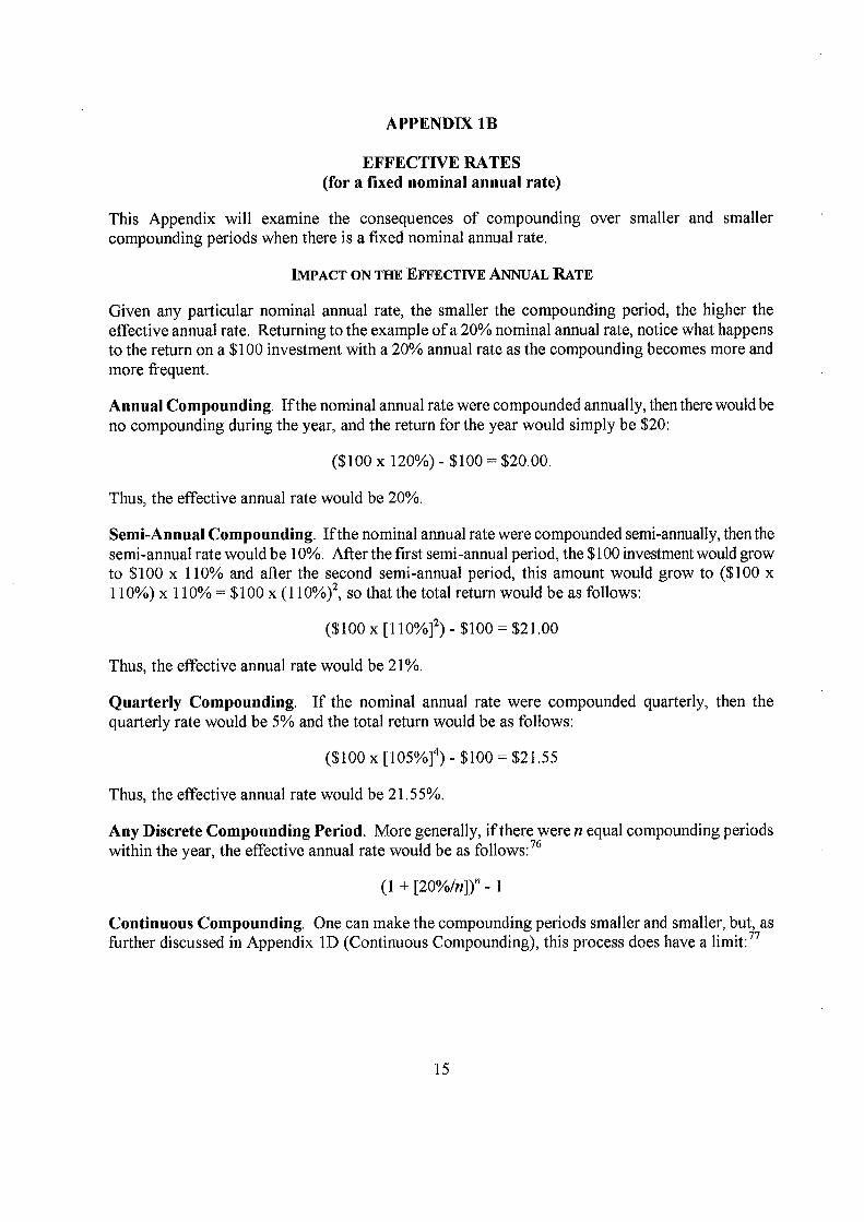
This Appendix will examine the consequences of compounding over smaller and smaller compounding periods when there is a fixed nominal annual rate.

IMPACT ON THE EFFECTIVE ANNUAL RATE

Given any particular nominal annual rate, the smaller the compounding period, the higher the effective annual rate. Returning to the example of a 20% nominal annual rate, notice what happens to the return on a $100 investment with a 20% annual rate as the compounding becomes more and more frequent.

Annual Compounding. If the nominal annual rate were compounded annually, then there would be no compounding during the year, and the return for the year would simply be $20:

($lOOx 120%)-$100$20.00.

Thus, the effective annual rate would be 20%.

Semi-Annual Compounding. If the nominal annual rate were compounded semi-annually, then the semi-annual rate would be 10%. After the first semi-annual period, the $100 investment would grow to $100 x 110% and after the second semi-annual period, this amount would grow to ($100 x 110%) x 110% = $100 x (110%)2, so that the total return would be as follows:

($100 x [110%]2) -$100 = $21.00

Thus, the effective annual rate would be 21%,

Quarterly Compounding. If the nominal annual rate were compounded quarterly, then the quarterly rate would be 5% and the total return would be as follows:

($100 x [105%]) - $100 = $21.55

Thus, the effective annual rate would be 2 1.55%.

Any Discrete Compounding Period. More generally, if there were n equal compounding periods within the year, the effective annual rate would be as follows: 76

(1 + [20%/n]) - 1

Continuous Compounding. One can make the compounding periods smaller and smaller, but, as further discussed in Appendix 1D (Continuous Compounding), this process does have a limit: 77

15

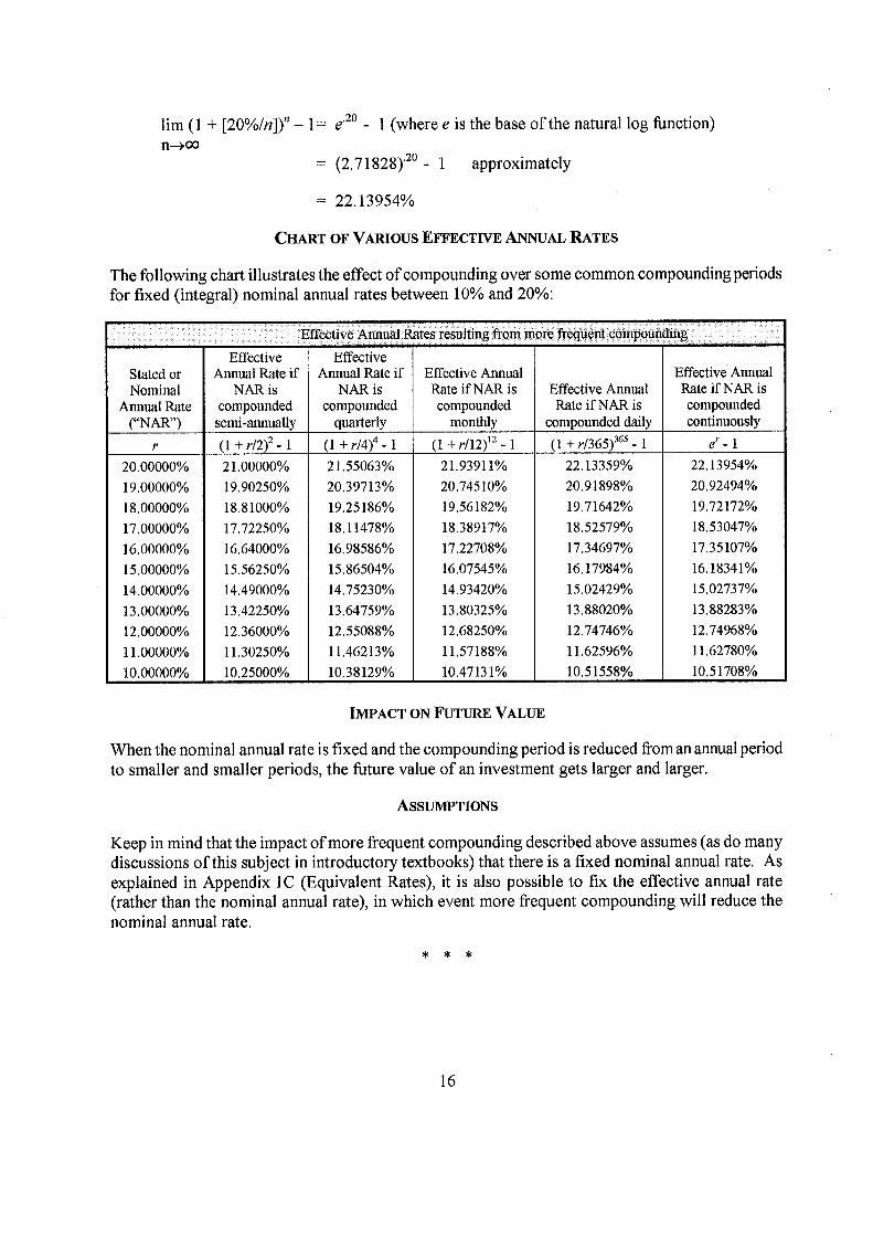
urn (1 + [20%1n]) - 1= e’20 - 1 (where e is the base of the natural log function) n-+OQ

= (2,71828)20 - 1 approximately

= 22.13954%

CHART OF VARIOUS EFFECT WE ANNUAL RATES

The following chart illustrates the effect of compounding over some common compounding periods for fixed (integral) nominal annual rates between 10% and 20%:

Effective Annual Rates resulting from more, frequent compour’ing

Effective Effective Stated or Animal Rate if Annual Rate if Effective Annual Effective Annual Nominal NAR is NAR is Rate if NAR is Effective Annual Rate if NAR is

Annual Rate compounded compounded compounded Rate if NAR is compounded ("NAR") semi-annually quarterly monthly compounded daily continuously

r (1+r/2)2 -1 (1+r/4)4 -1 (1+r112)’2 -1 (l+r/365)5-1 er_i

20.00000% 21,00000% 21.55063% 21.93911% 22.13359% 22,13954%

19.00000% 19.90250% 20.39713% 20,74510% 20.91898% 20,92494%

18.00000% 18.81000% 19.25186% 19.56182% 19.71642% 19.72172%

17.00000% 17.72250% 18,11478% 18.38917% 18.52579% 18.53047%

16.00000% 16.64000% 16.98586% 17.22708% 17.34697% 17.35 107%

15.00000% 15.56250% 15.86504% 16.07545% 16,17984% 16.18341%

14.00000% 14.49000% 14.75230% 14.93420% 15.02429% 15.02737%

13.00000% 13.42250% 13,64759% 13.80325% 13.88020% 13.88283%

12.00000% 12.36000% 12.55088% 12.68250% 12.74746% 12.74968%

11.00000% 11.30250% 11.46213% 11.57188% 11.62596% 11.62780%

10.00000% 1 10.25000% 1 10.38129% 1 10.47131% 1 10.51558% 1 10.51708%

IMPACT ON FUTURE VALUE

When the nominal annual rate is fixed and the compounding period is reduced from an annual period to smaller and smaller periods, the future value of an investment gets larger and larger.

ASSUMPTIONS

Keep in mind that the impact of more frequent compounding described above assumes (as do many discussions of this subject in introductory textbooks) that there is a fixed nominal annual rate. As explained in Appendix 1C (Equivalent Rates), it is also possible to fix the effective annual rate (rather than the nominal annual rate), in which event more frequent compounding will reduce the nominal annual rate.

* * *

16

APPENDIX 1C

EQUIVALENT RATES (for a fixed effective annual rate)

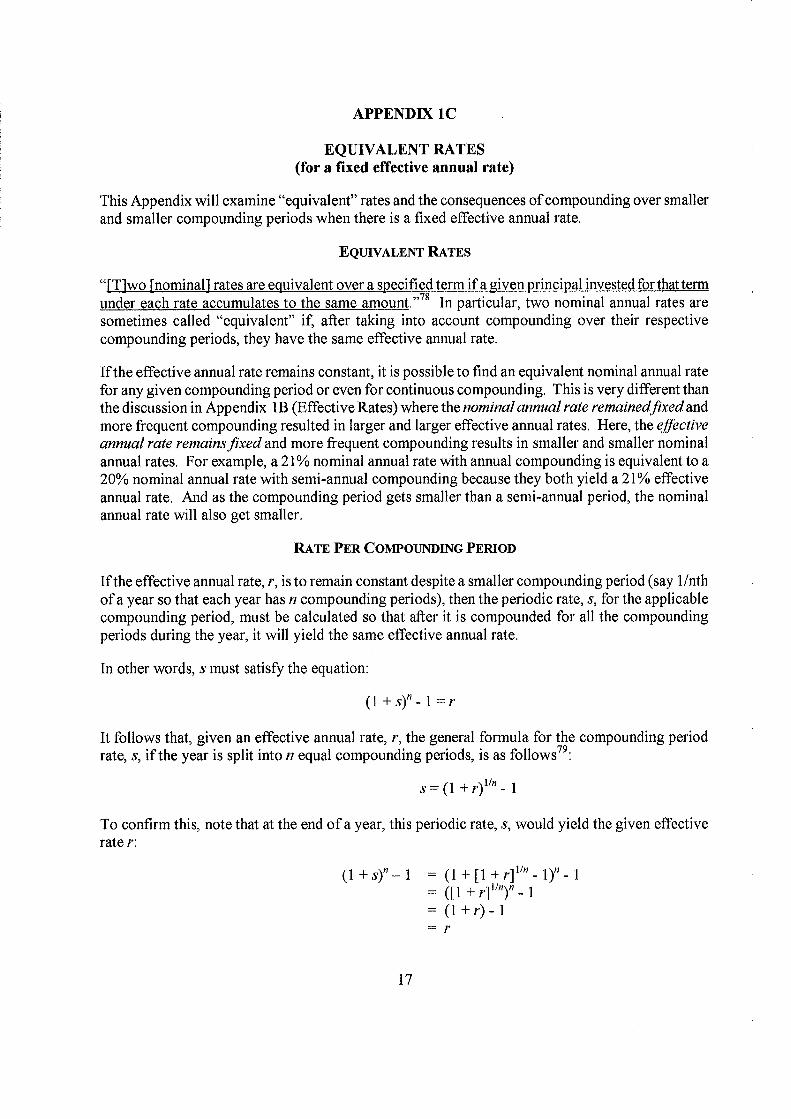
This Appendix will examine "equivalent" rates and the consequences of compounding over smaller and smaller compounding periods when there is a fixed effective annual rate.

EQUIVALENT RATES

"[T]wo [nominal] rates are equivalent over a specified term if a given principal invested for that term under each rate accumulates to the same amount, ,78 In particular, two nominal annual rates are sometimes called "equivalent" if, after taking into account compounding over their respective compounding periods, they have the same effective annual rate.

If the effective annual rate remains constant, it is possible to find an equivalent nominal annual rate for any given compounding period or even for continuous compounding. This is very different than the discussion in Appendix 1 B (Effective Rates) where the nominal annual rate remainedfixed and more frequent compounding resulted in larger and larger effective annual rates. Here, the effective annual rate remains fixed and more frequent compounding results in smaller and smaller nominal annual rates. For example, a 21% nominal annual rate with annual compounding is equivalent to a 20% nominal annual rate with semi-annual compounding because they both yield a 21% effective annual rate. And as the compounding period gets smaller than a semi-annual period, the nominal annual rate will also get smaller.

RATE PER COMPOUNDING PERIOD

If the effective annual rate, r, is to remain constant despite a smaller compounding period (say 1/nth of a year so that each year has n compounding periods), then the periodic rate, s, for the applicable compounding period, must be calculated so that after it is compounded for all the compounding periods during the year, it will yield the same effective annual rate.

In other words, s must satisfy the equation:

(1 +s)- I =r

It follows that, given an effective annual rate, r, the general formula for the compounding period rate, s, if the year is split into n equal compounding periods, is as follows 79 :

s = (1 + r)hmn -

To confirm this, note that at the end of a year, this periodic rate, s, would yield the given effective rate r:

(1 +s)� 1 = (I+ [I +r]- 1)-= ([1 +r]’- I = (I +r) -

I

17

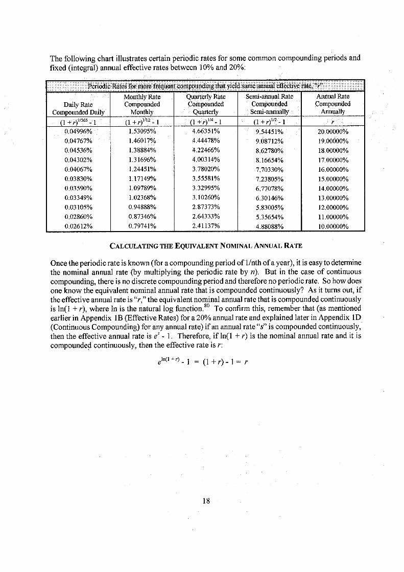
The following chart illustrates certain periodic rates for some common compounding periods and fixed (integral) annual effective rates between 10% and 20%:

Periodic Rates for more frequent compounding that yield same annual effective rate ’Y Monthly Rate Quarterly Rate Semi-annual Rate Annual Rate

Daily Rate Compounded Compounded Compounded Compounded Compounded Daily Monthly Quarterly Semi-annually Annually

(1 +r) 365 - 1 (1 +p)m2_ 1 (1 +r)114 _ 1 (1 +r) 2 - 1 r 0,04996% 1,53095% 4.66351% 9.54451% 20.00000% 0.04767% 1.46017% 4.44478% 9.08712% 19,00000% 0.04536% 1.38884% 4.22466% 8,62780% 18.00000% 0.04302% 1.31696% 4.00314% 8.16654% 17.00000% 0.04067% 1.24451% 3,78020% 7.70330% 16,00000% 0.03830% 1.17149% 3.55581% 7.23805% 15.00000% 0.03590% 1.09789% 3.32995% 6.77078% 14.00000% 0.03349% 1.02368% 3.10260% 6.30146% 13.00000% 0.03105% 0,94888% 2,87373% 5.83005% 12.00000% 0,02860% 0,87346% 2.64333% 5.35654% 11.00000% 0.02612% 1 0.79741% 2.41137% 4,88088% 1 10.00000%

CALCULATING THE EQUIVALENT NOMINAL ANNUAL RATE

Once the periodic rate is known (for a compounding period of 1/nth of a year), it is easy to determine the nominal annual rate (by multiplying the periodic rate by n). But in the case of continuous compounding, there is no discrete compounding period and therefore no periodic rate. So how does one know the equivalent nominal annual rate that is compounded continuously? As it turns out, if the effective annual rate is "r," the equivalent nominal annual rate that is compounded continuously is ln(1 + r), where In is the natural log function. 80 To confirm this, remember that (as mentioned earlier in Appendix I (Effective Rates) for a 20% annual rate and explained later in Appendix 1D (Continuous Compounding) for any annual rate) if an annual rate "s" is compounded continuously, then the effective annual rate is eS - 1. Therefore, if ln(1 + r) is the nominal annual rate and it is compounded continuously, then the effective rate is r:

e1°1 +r) - = ( 1 + r) - I = r

18

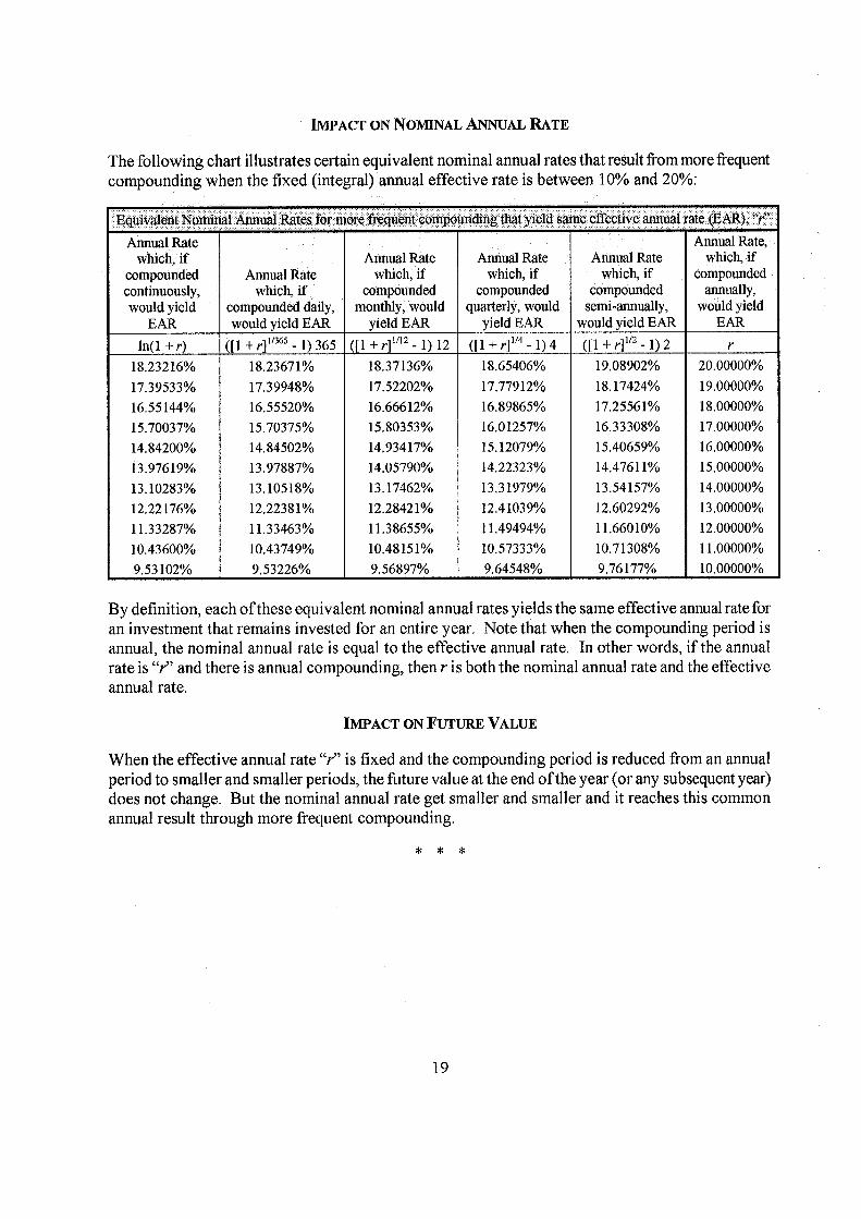
IMPACT ON NOMINAL ANNUAL RATE

The following chart illustrates certain equivalent nominal annual rates that result from more frequent compounding when the fixed (integral) annual effective rate is between 10% and 20%:

Equivalent Nominal Annual Rates for more frequent compounding that yield same effective annual rate (EAR), " r"

Annual Rate Annual Rate, which, if Annual Rate Annual Rate Annual Rate which, if

compounded Annual Rate which, if which, if which, if compounded continuously, which, if compounded compounded compounded annually, would yield compounded daily, monthly, would quarterly, would semi-annually, would yield

EAR would yield EAR yield EAR yield EAR would yield EAR EAR

ln(l + r) ([1 + r]"365 - 1) 365 ([1 + r]" 2 - 1)12 ([1 + r]"4 - 1) 4 ([1 + r]"2 - 1) 2 r

18.23216% 18.23671% 18.37136% 18.65406% 19.08902% 20.00000%

17.39533% 17.39948% 17.52202% 17.77912% 18.17424% 19.00000%

16.55 144% 16.55520% 16.66612% 16.89865% 17.25561% 18.00000%

15.70037% 15.70375% 15.80353% 16.01257% 16.33308% 17.00000%

14.84200% 14.84502% 14.93417% 15. 12079% 15.40659% 16.00000%

13.97619% 13.97887% 14.05790% 14.22323% 14.47611% 15.00000%

13.10283% 13,10518% 13.17462% 13.31979% 13.54157% 14,00000%

12.22176% 12.22381% 12.28421% 12.41039% 12,60292% 13.00000%

11,33287% 11.33463% 11.38655% 11.49494% 11.66010% 12.00000%

10.43600% 10.43749% 10.48151% 10.57333% 10.71308% 11,00000%

9.53 102% 9.53226% 1 9.56897% 1 9.64548% 1 9.76177% 1 10.00000%

By definition, each of these equivalent nominal annual rates yields the same effective annual rate for an investment that remains invested for an entire year. Note that when the compounding period is annual, the nominal annual rate is equal to the effective annual rate. In other words, if the annual rate is "r" and there is annual compounding, then r is both the nominal annual rate and the effective annual rate.

IMPACT ON FUTURE VALUE

When the effective annual rate "r" is fixed and the compounding period is reduced from an annual period to smaller and smaller periods, the future value at the end of the year (or any subsequent year) does not change. But the nominal annual rate get smaller and smaller and it reaches this common annual result through more frequent compounding.

* * *

19

APPENDIX 1D

CONTINUOUS COMPOUNDING (er as a limit)

This Appendix concerns the following limit (where "r" represents the applicable interest rate and "n" represents an integer):

\P1

11+�i =e urn I n) fl --- ), oo

which appears in Appendix I (Effective Rates) for the particular case where r 20%. This result follows 1 from the more general fact that (assuming "x" represents a real number):

/ \X I I r lim 1+� =e

x�*ce x)

which is explained in many, if not most, basic calculus textbooks 82 , although sometimes the discussion is limited to the case where x = n, as originally written above, For those readers who desire further background on this limit, this Appendix is intended to provide some preliminary guidance and identify some reference materials for more detail.

THE FIRST STEP (WHEN r =100%) - MEANING OF e

To verify that the limit in question equals er, it is of course necessary to know what e means. Most high school students are taught that e is a number, between 2 and 3, which is approximately 2.718. It is an irrational number, which means that it cannot be expressed as the quotient of two integers, rn/n. Equivalently, the irrationality of e means that it is an infinite decimal which (unlike 1/3 and other rational numbers that are infinite decimals) does not repeat. Obviously, one cannot simply write out an infinite non-repeating decimal, so e must be defined by some other means. But however it is defined, if the limit in question is correct, then e must equal this limit in the case when r = 1 (i.e., when the applicable interest rate is 100%):

( i’ . ( iY lim 1,,1+_) = lirn = e

X fl-9cfJ fl

Before establishing the more general result for any rater, many books 83 first establish the case above where r = 1, and the proof of this first step often depends on the manner in which e is defined.

ALTERNATIVE DEFINITIONS OF e

A review of mathematical textbooks reveals that the number e has various interesting properties, many of which may be and are, in fact, used as alternative definitions (from which the other properties may be derived). Here are some alternative definitions :84

20

The Limit Itself. Some textbooks" define e as the limit in question (when r = 1):

( iY1 = hm e fl �+cI fl

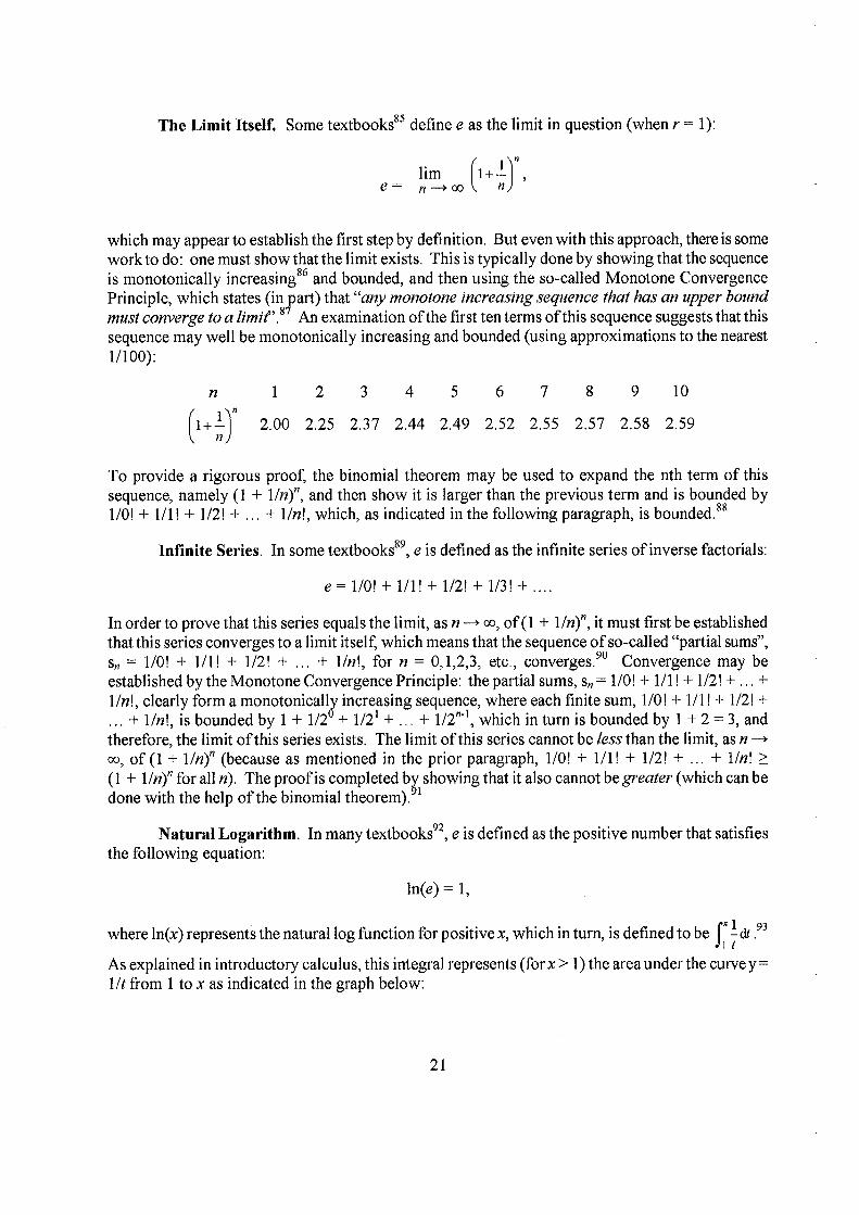
which may appear to establish the first step by definition. But even with this approach, there is some work to do: one must show that the limit exists. This is typically done by showing that the sequence is monotonically increasing 86 and bounded, and then using the so-called Monotone Convergence Principle, which states (in part) that "any monotone increasing sequence that has an upper bound must converge to a limit", 8 An examination of the first ten terms of this sequence suggests that this sequence may well be monotonically increasing and bounded (using approximations to the nearest 1/100):

n 1 2 3 4 5 6 7 8 9 10 / \fl

11+�i 2.00 2.25 2.37 2.44 2.49 2.52 2.55 2.57 2.58 2.59 n)

To provide a rigorous proof, the binomial theorem may be used to expand the nth term of this sequence, namely (1 + 1/n)’1 , and then show it is larger than the previous term and is bounded by 1/0! + 1/1! + 1/2! + ... + 11n!, which, as indicated in the following paragraph, is bounded. 88

Infinite Series. In some textbooks", e is defined as the infinite series of inverse factorials:

e= 1/0! + 1/1! + 1/2! + 1/3! +

In order to prove that this series equals the limit, as n �> cc, of (I + 11n)’1 , it must first be established that this series converges to a limit itself: which means that the sequence of so-called "partial sums", s, = 1/0! + 1/1! + 1/2! + ,,, + 11n!, for n = 0,1,2,3, etc., converges. 90 Convergence may be established by the Monotone Convergence Principle: the partial sums, s, = 1/0! + 1/1! + 1/2! +,.. + 1/n!, clearly form a monotonicall’ increasing sequence, where each finite sum, 1/0! + 1/1! + 1/2! +

+ 11n!, is bounded by 1 + 1/2 + 1/2’ + ... + 1/2’, which in turn is bounded by 1 + 2 = 3, and therefore, the limit of this series exists. The limit of this series cannot be less than the limit, as n cc, of (1 + 11n)’1 (because as mentioned in the prior paragraph, 1/0! + 1/1! + 1/2! + ... + 1/n! ? (1 + 1/n)’1 for all n). The proof is completed b showing that it also cannot be greater (which can be done with the help of the binomial theorem).

Natural Logarithm. In many textbooks 92, e is defined as the positive number that satisfies the following equation:

ln(e) = 1,

where ln(x) represents the natural log function for positive x, which in turn, is defined to be &

As explained in introductory calculus, this integral represents (for x> 1) the area under the curve y = lit from 1 to x as indicated in the graph below:

21

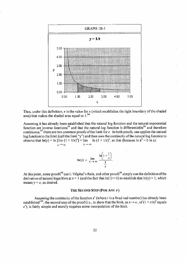
GRAPH lB-i

Thus, under this definition, e is the value for x (which establishes the right boundary of the shaded area) that makes the shaded area equal to 1. 94

Assuming it has already been established that the natural log function and the natural exponential function are inverse functions 95 and that the natural log function is differentiable 96 and therefore continuous, 97 there are two common proofs of the limit for e. In both proofs, one applies the natural log function to the limit (call the limit "y") and then uses the continuity of the natural log function to observe that In(y) = In [lim (1 + 1/x)x] = lim In (1 + 1/x), so that (because In ab = b In a):

x*oo x�cJ3

In(y) - +)

- QO 1

x

At this point, some proofs 98 use L’Hôpital’ s Rule, and other proofs 99 simply use the definition ofthe derivative of natural logarithm at x = 1 (and the fact that In(l) = 0) to establish that In(y) = 1, which means = e, as desired.

THE SECOND STEP (FOR ANY r)

Assuming the continuity of the function x’ (where r is a fixed real number) has already been established’00, the second step of the proof (i.e., to show that the limit, as x� 00, of (I + r/x)x equals e’), is fairly simple and merely requires some manipulation of the limit.

22

By substituting a new variable, z = (which implies that x = rz), (I+r.J may be written asx >00

lim -

I+ r ) which can be rewritten as [(ii) ] which equals I (1+1) ]

r

because r00

is continuous. 101 The desired result now immediately follows from Step 1 above.

* * *

23

ENDNOTES

See Carey, "Real Estate JV Promote Calculations: Basic Concepts and Issues", The Real Estate Finance Journal (Spring 2003) at 22; Carey, "Real Estate JV Promote Calculations: Recycling Profits", The Real Estate Finance Journal (Summer 2006) at 5: Carey, "Real Estate JV Promote Calculations: Catching Up with Soft Hurdles", The Real Estate Finance Journal (Spring 2008) at 8.

2 Kellison, THE THEORY OF INTEREST (3rd ed., McGraw-Hill 2009), § 7.9 at 282.

Geitner Miller Clayton Eicltholtz, COMMERCIAL REAL ESTATE ANALYSIS & INVESTMENTS (2nd ed., Cengage Learning 2007) § 8.1.4 at 153.

4 Brueggeman Fisher, REAL ESTATE FINANCE AND INVESTMENTS (1 0 ed., McGraw-Hill Irwin 2011), Ch. 3 at 54 n.2. See also 46-47 ("It is customary in the United States to use [an annual] nominal rate of interest in contacts,. . . mortgage notes, and other transactions.... [T]he term interest rate means a nominal, annual rate of interest.").

Geitner, supra, § 17. 1.1 at 408 ("contract" rate), § 17.2.1 at 420 ("contract’ ’ rate) and 421 ("contractual" rate); Ross, Westerfield, Jordan, FUNDAMENTALS OF CORPORATE FINANCE (8th ed., McGraw-Hill Irwin 2008), § 6.3 at 166 ("stated" or "quoted" rate).

6 Donald, COMPOUND INTEREST AND ANNUITIES-CERTAIN (2nd ed., Cambridge University Press 1970), § 2.3 at 8 (emphasis in original); See also Skinner, THE MATHEMATICAL THEORY OF INVESTMENT (Rev. ed., Gina and Company 1924), Ch. V, § 35 at 57 ("...the nominal [annual] rate.,, is the [annual] rate named in the contract and indicates what the return on one dollar would be if no interest ...during the year were to be reinvested [i.e., compounded] until the end of the year."). Note that Donald and Skinner refer to interestpayable or received (rather than compounded) during the year, but both appear to assume that the compounding and payment periods are the same, because they treat, for example, "payable quarterly", "compounded quarterly", and "convertible quarterly" as identical phrases. Donald, supra, § 2.3 at 8; Skinner, supra, § 33 at 51.

Steiner, MASTERING FINANCIAL CALCULATIONS (2nd ed., Prentice Hall 2007), Part 1 at 11 (emphasis in original).

8 See Ruckman and Francis, FINANCIAL MATHEMATICS (2nd ed., BPP 2005), § 4.2 at 100 ("A nominal interest rate is expressed as an annualized rate by multiplying the ... rate of interest [for the compounding period, lip of a year,] by the number of time periods, p. For example if the ... monthly rate of interest is 0,3%, then the nominal interest rate based on monthly compounding of interest is 0.3% x 12 = 3.60/o").

Geltner, supra, § 8.1,4 at 153. See also, Butcher and Nesbitt, MATHEMATICS OF COMPOUND INTEREST (1971. Reprint, Ulrich’s 1979), § 1.6 at 8; Adams Booth Bowie Freeth, INVESTMENT MATHEMATICS (Wiley 2003), § 1.3 at 5-6. For potential ambiguity regarding the use of the word "nominal", see text at endnote 39.

10 Kellison, supra, § 1.8 at 23 ("For example, a nominal rate of 8% [compounded] quarterly [means] an interest rate of 2% per quarter"; Butcher and Nesbitt, supra, §1.6 at 7 ("For example, the rate may be 4% per year [compounded] quarterly. This implies that the ... rate ... per quarter is 1%.").

See Geltner, supra, § 9.2.4. See also Ross, supra, § 7.6; Brealey, Myers, Allen, PRINCIPLES OF CORPORATE FINANCE (10 th ed., McGraw-Hill Irwin 2011) § 3.5. This article does not address "real" returns or otherwise deal with the impact of inflation.

12 See Geltner, supra, § 8.1.4 at 153 ("effective annual rate"); Brueggeman Fisher, supra, Ch. 3 at 45 ("effective annual yield"); and Ross, supra, § 6,3 at 166 ("effective annual rate"). For potential ambiguity regarding the use of the word "effective", see text at endnotes 41 and 42.

13 See, e.g., Day, MASTERING FINANCIAL MATHEMATICS IN MICROSOFT EXCEL (Pearson Education 2005), Ch. 2 at 25-26; Hewlett-Packard, HP 12C PLATINUM OWNER’S HANDBOOK AND PROBLEM-SOLVING GUIDE (Hewlett-Packard, 2003), § 15 at 157-159.

24

14 Rietz, Crathhorne, and Rietz, MATHEMATICS OF FINANCE (Henry Holt and Company, 1929), Ch. I, § 2 at 1; see also, Butcher and Nesbitt, supra, § 1,6 at 7; Kellison, supra, § 1.2 at 2; Broverman, MATHEMATICS OF INVESTMENT AND CREDIT (4th ed., Actex 2008), § 1.1 at 4. See also endnotes 3,4 and 71.

15 Vaaler & Daniel, MATHEMATICAL INTEREST THEORY (2nd ed., Pearson Education, Inc. 2009), § 1,3 at 11; McCutcheon and Scott, AN INTRODUCTION To THE MATHEMATICS OF FINANCE (1986. Reprint, Butterworth-Heinemann 2005), Ch. 2, § 2.1 at 10.

16 For a generalized discussion of nominal and effective rates, see McCutcheon and Scott, supra, §§ 2.1-2.3 at 10-14 (which basically provides a definition of nominal rate for each payment period, which could also be used for each compounding period, and allows for the possibility of a different interest rate for each period); but see Carey, "Effective Rates of Interest", The Real Estate Finance Journal (Winter 2011) at 11.

17 Brueggeman Fisher, supra, Ch. 3 at 72; Geltner, supra, § 8.1,4 at 153. 18 Zima Brown Kopp, MATHEMATICS OF FINANCE (6th ed., McGraw-Hill Ryerson, 2007), § 2,2 at 39 ("Two

nominal compound interest rates are equivalent if they yield the same accumulated values at the end of one year.."); Ruckman and Francis, supra, § 4,2 at 101; Hummel and Seebeck, MATHEMATICS OFFINANCE(3’’ ed., McGraw-Hill, 1971), Ch. 2, § 13 at 25 ("Any two interest rates, whether nominal or effective rates, that give the same compound amounts at the end of the year are called yearly equivalent or more briefly, equivalent"); Ayres, MATHEMATICS OF FINANCE (Schaum’s Outline Series, McGraw-Hill, 1963), Ch. 7 at 65 ("Two annual rates of interest with different conversion periods are called equivalent if they yield the same compound amount at the end of the one year."); Shao, MATHEMATICS OF FINANCE (South-Western Publishing Company 1962), § 105C at 254-255.

19 Brueggeman Fisher, supra, Ch. 3 at 43; Geltner, supra, §§ 8.1.1, 8.1.2; Ross, supra, § 5.1 at 122; Brealey, supra, § 2.1 at 21; Day, supra, Ch. 2 at 20; Steiner, supra, Part 1 at 12; Butcher and Nesbitt, supra, § 1.3; and Kellison, supra, § 1.6 at 14.

20 See, e.g., The Economist, NUMBERS GUIDE (5th ed., Bloomberg Press 2003) at 44 21 Brealey, supra, § 2,1 at 22; Kellison, supra, § 1.6 at 13-14, Present value may be defined more broadly, but the

definition given in this article is consistent with the presentation found by the author in most introductory reference books. See Kellison, supra, § 1.6 at 14.

22 Shim Henteleff, WHAT EVERY ENGINEER SHOULD KNOW ABOUT ACCOUNTING AND FINANCE (Marcel Dekker, Inc. 1995), Ch. 11 at 174; Geltner, supra, § 8.1.1 at 151; Ross, supra, § 5.2 at 129. This is not to be confused with the discount rate for borrowing where interest is paid in advance. Vaaler & Daniel, supra, § 1.6 ("discount rate"); Kellison, supra, § 1,7 at 15 ("effective rate of discount"); Broverman, supra, § 1.5.1 at 31-32 ("rate of discount"). For other uses of the word "discount", see text at endnote 38.

23 Geltner, supra, § 8.2 at 155-156; Shim, supra, Ch. 11 at 174; Benninga, FINANCIAL MODELING (2nd ed., MIT Press 2000), § 1.2 at 3-5.

24 See, e.g. Kellison, supra, § 7.2 at 251 (defining net present value with formula for present value of net cash flows, some of which may be positive and some of which may be negative); equivalently, sometimes all the cash flows are listed as positive amounts and the net present value is defined as the present value of the cash inflows less the present value of the cash outflows. See, e.g., Floyd Allen, REAL ESTATE PRINCIPLES (8th ed., Dearborn Financial Publishing 2005) Ch. 14 at 310; Ruckman and Francis, supra, § 5.1 at 128.

25 See, e.g., Brueggeman Fisher, supra, Ch. 3 at 58 (see "interest factors" used for future value calculations in Exhibits 3-8 and 3-9); Kellison, supra, § 1.2 at 2 (referring to "accumulation function" or "accumulated value"), § 1.6 at 13 (referring to "accumulation factor"); Ross, supra, § 5.1 at 123 (referring to "future value interest factor" or "future value factor"); Copeland, Weston, Shastri, FINANCIAL THEORY AND CORPORATE POLICY (4th ed.,Pearson Education, Inc. 2005), App. Dat 930 (referring to "future value interest factors"); and Appraisal Institute, THE APPRAISAL OF REAL ESTATE (1 I t" ed, Appraisal Institute 1996), App. C at 765 (referring to "future value factor").

26 See, e.g., Brueggeman Fisher, supra, Ch. 3 at 53-56 (referring to "present value interest factors" and using interest factors for present value calculations in Exhibits 3-6 and 3-7); Kellison, supra, § 1.6 at 13 (referring to

a "discount factor"); Ross, supra, § 5.1 at 131 (referring to "discount factor," "present value interest factor" or "present value factor"); Copeland, supra, App. Dat 930 (referring to "present value interest factors"); Appraisal ’Institute, supra, App. Cat 767 (referring to "present value factor"); and Brealey, supra, § 2.1 at 22 (referring to "discount factor").

27 Ruckman, supra, Ch. 4 at 95. 28 Ruckman, supra, Ch. 4 at 95. This is consistent with the assumption that compounding and cash flow periods

are the same. 29 Geltner,supra, § 17,1.1at408,fn, 1.

Geltner, supra, § 17. 1.1 at 408, fn. 1. 31 Geitner, supra, § 17.1.1 at 408-409, fn. 2 (and accompanying text). 32 Broverman, supra, § 5. 1.1 at 264-265; Kellison, supra, § 7.2 at 252; Ruckman, supra, § 5.1 at 130; Ross, supra,

§ 9.5 at 277-288; Brealey, supra, § 5.3 at 107-108.

See, e.g., Brovennan, supra, § 5. 1.1 at 265; Ruckman, supra, § 5.1 at 130; Zima, supra, § 7.2 at 243.

See, e.g., Frost, THE BANK ANALYST’S HANDBOOK (John Wiley & Sons, 2004) at23 (".. the internal rate of return is the discount rate that takes the value of the future cash payments back to the value of the initial investment"). Of course, the above quote is correct assuming "payments" means all "cash flows" whether positive inflows or negative outflows. Cf. Appraisal Institute, supra, Ch. 20 at 457 ("The internal rate of return for an investment is the yield rate that equates the present value of the future benefits of the investment to the amount of capital invested"); Brueggeman Fisher, supra, Ch. 11 at 358 ("the IRR ... is the rate that makes the present value of the projected cash flows equal to the initial investment").

cf. Broverman, supra, § 5.1.1 at 264-267.

Broverman, supra, § 2.4.1 at 126 ("... the internal rate of return on a loan transaction is simply the interest rate at which the loan is made"), and § 3.1,1, Def. 3.1 at 175; see also, Vaaler & Daniel, supra, § 3,6 at 133; Ruckman, supra, § 5.5 at 147.

Kellision, supra, §7.2 at 250. 38 Kellison, supra, § 1.7 at 20.

See Kellison, supra, § 1.8 at 26-27.

Shao, supra, § 10.513 at 251. See also discussion under the heading "ANNUAL RATES". 41 Floyd Allen, supra, Ch. 15 at 324 ("The term effective interest rate refers to the actual cost ofborrowingfunds

from a lender, expressed as an annual rate, after consideration of discount points and origination fees."); Ledgerwood, MICROFINANCE HANDBOOK (The World Bank, 1999), Ch, 5 at 143 ("The e[fective rate ofinterest refers to the inclusion of all direct financial costs of a loan in one interest rate"); Brueggeman Fisher, supra, Ch. 4, Concept Box 4.2, Note ’ at 98 ("effective interest rate"); Geltner, supra, § 17.2.1 at 421 ("effective interest rate"); see also endnote 45 below.

42 See Carey, "Effective Rates of Interest", The Real Estate Finance Journal (Winter 2011) at 11.

Ross, supra, § 6.3 at 168; accord; Brigham, Gapenski, FINANCIAL MANAGEMENT THEORY AND PRACTICE (5 th ed., The Dryden Press 1988), Ch. 4 at 106, fn. 8.

Kellison, supra, § 8.2 at 310; accord, Broverman, supra, § 3.2.2 at 194 ("The APR . . is nominal annual rate of interest compounded monthly ..."); Vaaler & Daniel, supra, § 1.10 at 44, fn. 5 ("APR ... is an acronym for ’annual percentage rate,’ used to indicate a nominal rate."); Fabozzi, Drake, FINANCE: CAPITAL MARKETS, FINANCIAL MANAGEMENT, AND INVESTMENT MANAGEMENT (John Wiley & Sons, 2009), Ch. 2 at 47 ("The APR ignores the effect of compounding").

Brueggeman Fisher, supra, Ch. 4, Concept Box 4.2, Note t at 98 ("Generally, the APR ... disclosed to the borrower is the effective interest rate"), and Ch. 4 at 99 ("... the effective interest rate ... will always be equal to the contract rate of interest when no finance charges are made at the time of loan origination or repayment");

Tel

Geitner, supra, § 17,2.1 at 421 ("The YTM from the lender’s perspective at the time of loan origination is often referred to as the ... APR ... [or] effective interest rate faced by the borrower"), and § 17.2.1 at 420 (where the authors conclude that a fully amortizing loan with monthly payments and an 8% nominal annual interest rate, but no origination fees or other charges that would be taken into account in determining the APR, has a’YTM of 8%). (For numerous books that refer to an effective rate of interest or effective rate as a rate that takes into account compounding, see Carey, "Effective Rates of Interest", supra.)

46 Shapiro, MODERN CORPORATE FINANCE (Macmillan Publishing Company 1990), Ch. II, § 2.1 at 30-31; see also, The Economist, supra, at 42 ("The effective [annual] rate must be quoted in the United States [to reflect compounding]").

See, e.g., Steiner, supra, Part 1 at 11 ("In the UK, for example, credit card companies are obliged to quote the effective rate [which is defined to take into account compounding] (known as APR, the annualised percentage rate)"); Directive 98/7/EC Feb. 16, 1998, Official Journal of the European Communities (1.4.98) L101/17-23, providing formula for APR for the European Union; Texas Instruments Business, BAlI Executive Calculator Guidebook (Texas Instruments, 1984), Ch. 6 at 6-1 ("The interest rate is generally stated as an effective rate in Europe. Nominal rates are most commonly used in the United States... The Annual Percent Interest Rate (APR) is essentially the same as the annual nominal rate"); European Union Committee, "Consumer Credit in the European Union: Harmonisation and Consumer Protection", 36th report of Session 2005-06, Vol. I Report (House of Lords 2006), Ch. 3, 160 at 21 ("The rules on the APR embody [the principle] ... that the total charge for credit should be expressed not only as a nominal rate (i.e., one which ignores the frequency of compounding) but as an effective annual percentage rate ..."); Sijthoff, CONSUMER CREDIT, United Kingdom Comparative Law Series, Vol. 3 (Eastern Press, 1978), Part I, Ch. 5 at 55 (see footnote 12 and accompanying text, indicating that at the time, the U. S. required disclosure of a nominal rate and the United Kingdom and apparently, Germany and France, required disclosure of an effective annual rate).

48 Ross, supra, § 63 at 168-169.

Kellison, supra, § 1.7 at 20. 50 Ruckman, supra, § 5.1 at 130. See also example on that page. See also, Lusztig Cleary Schwab, FINANCE IN A

CANADIAN SETTING (6th ed., John Wiley & Sons 2001), § 5.2 at 154, which equates the internal rate of return with the effective annual interest rate, although this is in the context of an example with annual cash flows.

Lynch, FINANCIAL MODELING FOR PROJECT FINANCE (Euromoney Publications 1996), Workbook 2 at 52; see also, Edleson, VALUE AVERAGING: THE SAFE AND EASY STRATEGY FOR HIGHER INVESTMENT RETURNS (John Wiley & Sons 2007), at 29 (which, in an example with monthly cash flows, says "the internal rate of return (IRR) is 0.33% monthly, which is 4.03% annually" (which is the effective annual rate [1 +.33 0/.]" - 1)); see also, Fabozzi, FIXED INCOME MATHEMATICS

(4th ed., McGraw-Hill 2006), Ch. 5 at 60, Ch. 7 at 99, Ch. 11 at 186, but note that Fabozzi, states (at 99-100): "Although the proper way to annualize a semiannual interest rate is [by compounding], the convention adopted in the bond market is to double the semi-annual interest rate In fact, this convention is carried over to yield calculations for other types of fixed income securities." (footnote omitted; emphasis in original).

52 Stark, ENCYCLOPEDIA OF LOTUS 1-2-3 RELEASE 3, THE MASTER REFERENCE (Windcrest Books 1989), Ch. 3 at 359.

53 See, e.g., Hewlett-Packard, supra, § 4 at 63 ("Note that the value calculated by is the periodic rate of return. If the cash flow periods are other than years (for example, months or quarters), you can calculate the nominal annual rate of return by multiplying the periodic JRR by the number of periods per year".); Lima, DEVELOPING PARADOX 4.0 APPLICATIONS (Addison-Wesley Publishing 1993), Ch. 7 at 179 ("The internal rate of return will match the periodicity. That means if your periods are months, the program will return a monthly IRR. Multiply the rate returned by 12 to get the equivalent annual IRR"); but see Walkenbach, EXCEL 2007 FORMULAS (Wiley Publishing, Inc. 2007) Ch. 12, Fig 12-12 at 334.

54

See e.g., Geltner, supra, § 8.2.14, fn. 11 at 167 (",.. the IRR may be reported on a per-period basis, so that, for example, if the periods were months, you would have to multiply the computed IRR by 12 to obtain the nominal per-annum rate"); Floyd Allen, supra, Ch. 15 at 325 (which solves for a monthly IRR and then calculates an annual IIRR by multiplying by 12).

27

Brueggeman Fisher, supra, Ch. 3 at 70. See also Broverman, supra, § 5.1,1, Example 5.1 at 266-267 (which is an example of an IRR quoted as a nominal annual rate for semi-annual cash flows: determining an "effective 6-month internal rate of return" equal to 3.246% "or equivalently", a nominal annual rate of "6.49%", which is 2 x 3.2461/o, compounded semi-annually).

Ledgerwood, supra, Ch. 5 at 148.

Ledgerwood, supra, Ch. 5 at 144.

Day, supra, Ch. 3 at 38.

Day, supra, Ch. 3 at 38-39; but see Walkenbach, supra, Ch. 12, Figure 12-12 at 334. 60 See, e.g., Stigum and Robinson, MONEY MARKET AND BOND CALCULATIONS (Irwin 1996), Ch. 5. 61 Kellison, supra, § 7.2 at 249 ("cash outflow from the investor into the investment"); Ruckman, supra, § 5.1 at

128 ("money is being paid out by the investor (cash outflows)"); Broverman, supra, § 5.1.1 at 264 ("cashflows Out (payments made)").

62 Kellison, supra, § 7.2 at 249 ("cash inflow from the investment to the investor"); Ruckman, supra, § 5.1 at 128 ("money is coming in to the investor (cash inflows)"); Broverman, supra, § 5.1.1 at 264 ("cashflows in (payments received)"). See also text at endnote 37.

63 Steiner, supra, Ch 1 at 21. Alternatively, it is possible to make cash outflows positive and cash inflows negative. See Kellison, supra, § 7.2 at 249, which effectively considers both approaches in the context of net cash flows.

64 See Broverman, supra, § 5,1.1 at 264-265; Ruckman, supra, § 5,1 at 128. 65 Adams, supra, § 1.7 at 15. See also, Broverman, supra, § 5. 1.1 at 264-265; Ruckman, supra, § 5.1 at 128. See

also Kellison, supra, § 7.2 at 249, ("The word net refers to the process of offsetting [cash inflows] and [cash outflows] at the same time.")

66 McCutcheon and Scott, supra, § 3.2 at 37 ("In most situations only one of [the cash outflows or cash inflows as of any given time] will be non-zero"),

67 See, e.g., Broverman, supra, § 5. 1.1 at 265 ("If a payment ,..is disbursed at [a particular time,] but there is no payment received at that time, then [the receipt at that time] = 0. Conversely, if there is a payment received.. at [a particular time,] but no payment disbursed at that time, then [the disbursement at that time] = 0").

65 See, e.g., Kellison, supra, § 7.2 at 249 where the assumption is implicit. 69 Kellison, supra, § 1.2 at 2.

McCutcheon & Scott, supra, § 2.1 at 10; see also, Vaaler & Daniel, supra, § 1,3 at 11. 71 Kellison, supra, § 1.2 at 2. See also, Vaaler & Daniel, supra, § 1,3 at 11; McCutcheon & Scott, supra, § 2.1 at

10, 72 See endnote 71.

C. Broverman, supra, § 1. 1.2 at 11.

Vaaler & Daniel, supra, § 1.7 at 34 and fn. 4 (" ...choose an increment of time between successive cash flows... [which] should in general be ... the longest time interval that allows you to include all your non-zero cash flows"); Kellison, supra, § 7.2 at 249 ("For convenience, we assume that these times [between cash flows] are equally spaced."); Geltner, supra, § 8.2.14, fn 10 at 166 ("If the cash flows occur at irregularly spaced points in time, one can simply define the smallest [sic] common time divisor as the period and have [the cash flows] = 0 between the cash flow receipts").

McCutcheon and Scott, supra, § 2.3 at 13; Broverman, supra, § 1. 1.2 at 10, Def. 1.3; Kellison, supra, § 1.2, formula 1,1 at 3; Vaaler & Daniel, supra, § 1.3 at 12.

76 See Brealey, supra, § 2.4 at 36; Copeland, supra, App. A at 888-889.

28

See Brealey, supra, § 2.4 at 36; Copeland, supra, App. A at 889-890; Vaaler & Daniel, supra, § 1.13 at 57; Zima, supra, § 2.9 at 68-71; Cissell Cissell Flaspohier, MATHEMATICS OF FINANCE (gth ed., Houghton Muffin 1990) § 3.22 at 183-185.

78 Butcher and Nesbitt, supra, § 1.7 at 9-10; see also, endnote 18.

Broverman, supra, § 1.4.1 at 29. 80 Broverman supra, § 1.6.3 at 43-44, Kelhson supra App 1 at 40-41 Steiner, supra Part 1 at 8-9 81 Shilov, ELEMENTARY REAL AND COMPLEX ANALYSIS (Rev. English ed., Dover Publications 1996), § 4.65 at

125. 82 The relevant discussion will often be found by checking the subject index for "Interest", "Compounding" and

"Continuous Compounding", 83 But see the following books which provide proofs that are not split into these steps: Courant and John,

INTRODUCTION TO CALCULUS AND ANALYSIS, Vol. I (Interscience Publishers, 1965), Ch. 2, § 2.6c at 152, which uses the mean value theorem of integral calculus; Apostol, CALCULUS, Vol. 1(2nd ed., Wiley-India, 2006), § 7. 10, Example 4 at 290, which uses polynomial approximations to prove an equivalent result.

84 This is not intended to be a complete list, but these are definitions frequently encountered by the author. It is also possible, for example, to define e as the number for which the slope of bX is I at the origin. Rodin, BASIC

CALCULUS WITH APPLICATIONS (Goodyear Publishing Company, Inc. 1978), Ch. 5, § 3 at 190; Stewart, CALCULUS (6th ed., Thomson 2008), § 7.2, Def. 7 at 397 (but note that Stewart has alternative definitions).

85 Shilov, supra, § 4.63.d at 123-124 (using n instead of x); Maor, e: THE STORY OF A NUMBER (Princeton University Press 1994), Ch. 4 at 35 and Appendix 2 at 201-202 (using n instead of x); see also Finney, Weir and Giordano, THOMAS’ CALCULUS (Updated 10th ed., Pearson Education, Inc. 2003), Ch. P, § 3 at 27, which notes that e may be defined in this manner; Spivak, CALCULUS (3rd ed., Publish or Perish, Inc. 1994) Ch, 18, Exercise 32 at 354 (using the equivalent limit of (1 + h)hlh as h goes to 0), which "outlines the classical approach to logarithms and exponentials." For a criticism of this approach, see Klein, ELEMENTARY

MATHEMATICS FROM AN ADVANCED STANDPOINT (translated from 3rd German ed., Dover Publications 2004), Part Three, 1.1 at 146 (using n instead of x).

86 A sequence "is called monotonically increasing if each term ... is larger, or at least not smaller than the preceding one..." Courant and John, supra, § 1.7c at 74. See also, Rudin, PRINCIPLES OF MATHEMATICAL

ANALYSIS (3rd ed., McGraw-Hill 1976), Ch. 3, Def. 3.13 at 55; cf Stewart, supra, § 12. 1, Def. 10 at 717. 87 Courant and Robbins, WHAT IS MATHEMATICS? (2 ed., Oxford University Press 1996), Ch. 6, § 2 at 295;

Rudin, supra, Ch. 3, Theorem 3,14 at 55; Shilov, supra, § 4.63.c at 123; Levi, POLYNOMIALS, POWER SERIES

AND CALCULUS (D. Van Nostrand Company, Inc., 1968), Ch. 5, Theorem 5-1 at 82; Stewart, supra, § 12. 1, Theorem 12 at 719,

88 See Shilov, supra, § 4.63.d at 123-124; Spivak, supra, Exercise 32 at 354; see Maor, supra, Ch. 4 at 35 and Appendix 2 at 201-202.

89 Courant and John, supra, § 1.7e at 77; Rudin, supra, Ch. 3, Def. 3.30 at 63. 90 See, e.g., Rudin, supra, § 3.29 at 59; Shilov, supra, § 6.11 at 186. 91 Courant and John, supra, § 1.7e at 77-80; Maor, supra, Appendix 2 at 202; Rudin, supra, Ch. 3, Def. 3.30 at 63. 92 See, e.g., Apostol, supra, Ch. 6, § 6.5, Def. 6.11 at 231; Thomas, Finney, CALCULUS AND ANALYTIC

GEOMETRY (6th ed., Addison-Wesley 1984), Ch. 6, § 6.6 at 407; Larson, Hostetler, Edwards, CALCULUS OF A SINGLE VARIABLE (5th ed., D. C. Heath and Company 1994), Ch. 5, § 5.1 at 320; Stewart, supra, § 7.2*, Def. 5 at 424 (but note that Stewart has alternative definitions for e). Equivalently, some textbooks define e to be exp(1) where exp(x) is defined to be the inverse of the natural log function. Finney, supra, Ch. 6, § 6.2 at 468; Spivak, supra, Ch. 18 at 340.

29

See, e.g., Apostol, supra, Ch. 6, § 6.3, Def. 6.7 at 229; Thomas, Finney, supra, Ch. 6, § 6.4 at 394; Larson, supra, Ch. 5, § 5.1 at 317; Stewart, supra, § 7,2*, Def. 1 at 421 (but note that Stewart has alternative definitions for ln(x)); Finney, supra, § 6.1 at 457; Spivak, supra, Ch. 18 at 338.

See, e.g., Reid, FROM ZERO To INFINITY: WHAT MAKES NUMBERS INTERESTING (6th ed., A K Peters, Ltd. 2006), at 155. Reid’s book does not require any mathematical background and does not provide a proof of the limit in question, but simply notes (in footnote 3 at 155-156): "We can also characterize e in the following down-to-earth manner: If we invest $1.00 at 100 percent interest compounded continuously, at the end of one year we shall have $2.72 �that is, e dollars."

This is typically done by definition. Usually, one of these functions is defined and then the other function is defined as its inverse. See, e.g., Stewart, supra, § 7.3, (1) at 405 and (5) at 406 (after defining exp(x), ln(x) is defined to be its inverse), § 73*, (1) at 430 (after defining ln(x), exp(x) is defined to be its inverse).

96 When ln(x) is defined in the manner described in the body of this Appendix, it immediately follows from the (first) fundamental theorem of Calculus that In(x) is differentiable and its derivative is lIx. See, e.g. Apostol, supra, § 6.3, Theorem 6.1(b) at 229; Stewart, supra, § 7,2*, (2) at 422.

Any differentiable function is continuous. See, e.g., Apostol, supra, § 4.4, Example 7 at 163.

Stewart, supra, § 7.8, leaves this as Exercise 85 at 480. When L’Hôpital’s Rule is used, it is easier to examine the equivalent limit, as x tends to 0 from above, of (1 + x) 1 , as is done in Thomas, Finney, supra, § 6.6, Example 8 at 420-421. But see Spivak, supra, Ch. 18, Exercise 16(a) at 351, where it states that it would be silly to use L’Hôpital’s Rule.

Larson, supra, § 5.5, Theorem 5.15 at 357 and Appendix A at AlO-Al 1, which substitutes (for 11x and notes that the resulting equivalent limit, as (tends to 0 from above, of [ln( 1 + t) - 0]1t, is the derivative of the natural log function (1/x) at x = 1, namely 1. Many books first prove that the limit, ash tends to 0, of (1 + h)’ 1h equals e, from which the desired result immediately follows by substituting 11x or 1/n for h. Finney, supra, § 6.2 at 471; Stewart, supra, § 7,4* at 444; see also, Spivak, supra, Ch. 18, Exercise 16(a)-(c) at 351, Answers at 638-63 9, which relies on the continuity of exp(x).

°° If the natural log function is defined in the manner described in the body of this Appendix and exp(x) is defined as its inverse, then the natural exponential function is continuous because the natural log function is continuous,

and the function xr = e e, is continuous because it is a composite function made up of continuous functions. See, e.g., Larson, supra, § 5.3, Theorem 5.8.1 at 339 and Appendix A at A9-A10 (for continuity of inverse functions), and § 1. 2, Theorem 1.5 at 73, § 1.4 Theorem 1.12 at 89, Appendix A at A3 (for the continuity of composite functions). See also, Shilov, supra, § 5.53 at 150-151 for the continuity of x,r after defining e to be the limit, as n - , of (1 + 1/n) (which limit, as noted earlier, is equal to 1/0! + 1/1! + 1/2! + 1/3!+...).

101 Larson, supra, § 5.5 at 357; Finney, supra, § 6.2, Exercise 67 at 475 and Answers at A-36; Stewart, supra, § 7.5 at 451-452; Thomas, Finney, supra, § 6.10 at 437.

* * *

30

Copyright © 2011 Thomson Reuters. Originally appeared in the Spring 2011 issue ofThe Real Estate Finance Journal. For more information on the publication, please visithttp://west.thomson.com. Reprinted with permission.