1

Reforming the Speed of Justice:

Evidence from an Event Study in Senegal

Florence Kondylis and Mattea Stein*1

Preliminary & Incomplete

This Version: June, 2017

Can changing the rules of the game affect judges’ performance? We study the effect of a simple

procedural reform on the celerity of civil and commercial adjudication in Senegal. The reform gave

judges the duty and powers to meet a clear deadline. We combine the staggered rollout across the six

civil and commercial chambers of the court of Dakar and high-frequency caseload data to construct

an event study. We find a large reduction in the length of the pre-trial stage of 35-46 days (0.24-0.32

SD). The effect is similar for small and large cases, and is attributable to an increase in the

decisiveness of each hearing: the number of case-level pre-trial hearings is reduced, as judges are

more likely to set hard deadlines. These gains in speed do not come at the cost of quality, while we

document positive firm-level welfare impacts.

Keywords: Judiciary, Litigation Process, Efficiency, Bureaucracy, Public Organization, Public

Administration, Economic Development

JEL Classification: K41, D73, O12

* Florence Kondylis, Development Economics Research Group, World Bank: fkondylis@worldbank.org; Mattea Stein, Paris

School of Economics and EHESS: mattea.stein@psemail.eu . We thank Molly Offer-Westort, Violaine Pierre, Pape Lo, Felicité

Gomis and Chloe Fernandez for superb management of all court-level data entry and extraction. We are grateful to the

Ministry of Justice of Senegal and staff from the Economic Governance Project for their leadership in this work. We are

indebted to Presidents Ly Ndiaye and Lamotte of the Court of Dakar and their staff for making all court data available to us,

trusting our team throughout the process, and guiding us through the maze of the legal procedure. We benefited from advice

from high-level magistrates throughout the process, especially from Mandiogou Ndiaye and Souleymane Teliko. We also

thank George Akerlof, Kaushik Basu, Denis Cogneau, Klaus Decker, Pascaline Dupas, Marco Gonzalez-Navarro, Sylvie

Lambert, Arianna Legovini, John Loeser, Karen Macours, Jean-Michel Marchat, Thomas Piketty, Simon Quinn, Anne-Sophie

Robilliard, Dan Rogger, Paul Romer, Christopher Woodruff, Liam Wren-Lewis, Bilal Zia, for their insightful comments at

various stages of the project, as well as seminar participants at the 2015 ABCDE conference, the 2015 EUDN workshop,

Oxford University, the Paris School of Economics, and the World Bank. This research benefited from generous funding from

the EHESS Paris, KCP, RSB, the Senegal office of the World Bank, and the i2i fund and would not have been possible without

support from DIME. Edina Mwangi and Cyprien Batut provided superb research assistance. All usual disclaimers apply,

particularly that the views expressed in this paper do not engage the views of the World Bank and its members.

2

I. Introduction

Stronger institutions lead to higher levels of investments (Pande and Udry, 2006; Le, 2004;

Rodrik, 2000 and 2005), and capital accumulation drives a higher growth rate (Barro, 1991;

Mankiw, Romer, &Weil, 1992; Solow, 1956). Courts play a central role in strengthening

institutions, and the speed of justice is typically referred to as a key indicator of a country’s

institutional efficiency (Djankov et al., 2003; Lichand and Soares 2014; Alencar and

Ponticelli 2016; Visaria 2009). Whether to start or close a business, register property

(including intellectual), protect investors or enforce contracts, firms need to rely on the

legal system. Slow justice delivery is associated with a poorer business climate.

Yet, the evidence on policy options to cut legal delays is scant (Chemin, 2009b). Most legal

reforms are rolled out non-randomly across courts, judges or cases. Coupled with aggregate,

annual data, the evidence linking faster justice to investment often fails to establish

causality (Aboal et al., 2014). Perhaps more problematic, the quality tradeoffs and welfare

implications of speeding up adjudication have not, to this day, been empirically

documented.

Can changing the rules of the game affect judges’ performance? We combine micro data on

court cases and firms to document the causal impact of a legal reform on delays, quality of

adjudication, and firm-level welfare impacts. In 2013, Senegal’s Ministry of Justice

introduced a decree aiming to increase the celerity of civil and commercial adjudications.

The reform gave first-instance judges the duty and administrative powers to meet a

procedural deadline during the pre-trial stage of a trial. First, the decree set a four-month

limit on the duration of pre-trial hearings—which historically accounted for over two thirds

of the total duration of a case in first instance. Second, the reform imparted new

3

administrative powers to judges. Specifically, it encouraged judges to enforce submission of

supporting evidence from the outset and impose strict deadlines to the parties along the

pre-trial process. We combine a staggered administrative rollout across chambers of the

regional court with high-frequency case-level data to construct an event study and identify

the causal impact of the reform on the speed of justice.

This study makes four central contributions. First, we bring new evidence on the

determinants of judicial efficiency. Court-level studies tend to be circumscribed to richer

economies (Chang and Schoar, 2006), and have limited case-level data (Coviello et al.,

2015). In fact, the most granular data is typically judge-month statistics (Chemin,

2009a&b; Lichand and Soares, 2014; Alencar and Ponticelli, 2016). In contrast, we have full

access to bi-monthly audience and case-level data from the Regional Court of Dakar. We

build a high-frequency panel of all cases that entered the court between 2012/2015.2 For

each case, we retrace all procedures and hearings from entry to final judgment. This allows

us not only to document the impact of the reform on the overall speed of justice, but also

provide evidence on the underlying mechanisms and differentiate intensification from

increased decisiveness of the procedure.

Second, we innovate by proposing causal estimates of the impact of a judicial reform.

Chemin (2009a) uses yearly court-level data to identify the impact of a legal reform in

Pakistan, exploiting district-level variations in coverage. We use within-court variations in

coverage and high-frequency case and hearing-level data to construct an event study

around a change in legal procedure. This allows us to isolate the causal impact of the

reform on the speed of adjudication as well as quality and welfare impacts.

2 As the data becomes available, we will extend the analysis to include 2016 and investigate longer-

term effects.

4

Third, we add to the literature on public service reform by formally documenting the case-

level impact of a national change in civil and commercial procedure. We exploit a legal

reform that imposed deadlines on the duration of the purely administrative part of the trial

(pre-trial hearings) to study judges’ incentives and the drivers of procedural delays. We

follow Bandiera, Pratt and Valenti (2009) and apply a passive vs. active delays framework.

of pre-reform delays. Our main innovation is the richness of data we have access to in

documenting judges’ decisions along the judicial chain. This allows us to exploit both

changes in the distribution of delays and rich caseload data to identify the margin at which

procedural waste is reduced.

Last, we build evidence on the behavioral effects of deadlines. Delays in court may result

from strategic behavior on the judges’ part, whereby additional procedural time yields more

precise evidence or higher likelihood to extract rents. Alternatively, they may just be a

manifestation of irrational procrastination (Akerlof 1991). The reform we study is akin to

the deadline experiment proposed by Chetty et al. (2014) in which they manipulate the

delay for journal referees to complete their review. An important difference is that, in our

set-up judges are not explicitly reminded of the deadline at any point—hence not “nudged”

into action close to the deadline through the use of reminders. Instead, our results come

from a change in the default delay within which judges are expected to complete their pre-

trial hearings. Finally, we test for “tunnel vision” (Mullainathan and Shafir 2013), whereby

setting tight deadlines on one activity may increase the quality of the output subject to the

deadline, while reducing performance on other tasks.

We find the reform positively affected the speed of justice by both reducing formalism and

increasing the efficiency of the procedure. We find a large reduction in the length of the pre-

trial stage of 35-46 days (0.24-0.32 SD), as judges are 30.6-43.5% more likely to apply the

5

four-month deadline (an increase of 15.2-21.6 pp. from a baseline of 49.7%). We show that

this effect is attributable to an increase in the decisiveness of each hearing, as the number

of fast-tracked cases increases (23.8 percentage points), case-level pre-trial hearings are

reduced (0.21 SD), while judges are 40% more likely to set hard deadlines. We investigate

possible speed-quality tradeoffs, and find no evidence of judges’ effort displacement from

deliberations to pre-trial stages across all available measures: decision hearings are

scheduled at the same speed, the overall number of hearings does not increase, and the

quality of the evidence and the decision do not appear to be affected by the reform. We also

show that the decree does not affect parties’ intentions to appeal court decisions. Finally,

interviewing firms who used the court in our study period suggests positive welfare impacts

of the decree, both in a stated preference approach and comparing firm perceptions and

economic activity across the decree cutoff.

The remainder of the paper is organized as follows. We provide some element of background

on Senegal’s justice system and the legal civil and commercial procedure in Section 2.

Section 3 places the reform in the context of the Senegalese civil and commercial code of

procedure. Section 4 details the data; Section 5 presents the theoretical framework and

Section 6 the empirical strategy. Section 7 lays out our main empirical results, and Section

8 concludes.

II. Civil and commercial justice in Senegal

Senegal offers a good context to study the effect of a reform in court procedures, for three

reasons. First, Senegal is a civil law country, which implies a relatively a high degree of

formalism and, therefore, lengthy procedures (Djankov et al., 2003). Senegal ranked 142

6

out of 189 economies in the “contract enforcement” category of the 2014 Doing Business

Report, suggesting a significant margin of improvement in the speed of commercial dispute

resolution. We now detail the architecture of the court and legal procedure that make the

context of our study.

1. The court

Our study takes place in the regional court of first instance of Dakar, Senegal. Senegal is a

civil law country, and judges are organized in chambers, consisting of a president and two

additional judges (collegiality). While the court of Dakar adjudicates all types of affairs, we

focus on civil and commercial justice. At the beginning of our study period, in 2012, there

were 4 commercial and 3 civil chambers in the tribunal of Dakar. Tables 1 and 2 describes

the variations we have access to at the chamber and case levels, respectively.

Commercial and civil procedures in the tribunal of first instance consist of the following

general steps (see Annex A for a full schedule of the procedure): referral (saisine),

enrollment (enrôlement), distribution (répartition), pre-trial hearings (mise en état),

decision (délibération), and judgment (jugement). Referral and enrollment are purely

administrative steps that do not require the involvement of the judges. In 2012, 1546 new

civil and commercial cases were enrolled. Distribution consists in the assignment of the

new caseload to the chambers by the president of the court; it is notionally made on the

basis of existing caseload and, to a limited extent, the specialization of each chamber.

Chambers follow a schedule of hearings. Each chamber disposes of two dates per month on

which hearings can be scheduled. Each hearing opens with the assignment of new cases to

pre-trial judges, chaired by the president of the chamber. Next, each pre-trial judge chairs

her scheduled pre-trial hearings. Finally, the president of a chamber chairs decision

7

hearing, attended by the parties and all judges serving in that chamber (collégiale). On

average, a chamber takes in 16.4 new cases at each hearing (bi-monthly), ranging from 9.1

to 26.8 across chambers and years (Table 1).

Over the 2012/15 study period, two chambers closed: the 4th commercial in 2015, and the 2nd

civil in 2014. These closures led to increases in the size of the ongoing portfolio in other

chambers, as their ongoing cases were redistributed across the tribunal by the court

president. These changes in portfolio are uneven across chambers, due to a certain degree

of specialization of each chamber (Table 1).

Commercial and civil disputes vary widely in their nature and complexity. Commercial

cases include mostly payment and other contract disputes, including sale and rent contracts

involving a moral person (firm). Similarly, civil cases include contract and payment

disputes between individuals (e.g. landlord and tenant), as well as other civil issues like

divorces. 63% of civil and commercial disputes in our sample include a payment claim.

Among these, the average claim amount is of CFA 75,604,000 (or about 157,000 dollars),

ranging from CFA 75,000 to CFA 8,700,838,000 (about 160 dollars to 18,098,000 dollars;

Table 2).

2. Procedure

We now provide a simplified overview of the first instance civil and commercial procedure

in Senegal, focusing on the pre-trial hearing and decision stages leading up to the

publication of a judgment.

Pre-trial phase. At its first hearing, a case is assigned to a pre-trial judge by the president

of the chamber, starting the pre-trial phase. During this phase, the parties are invited to

8

build up their case. Pre-trial hearings are chaired by the assigned pre-trial judge.

Throughout this phase, the judge serves an administrative role. She is required to show

impartiality while the parties are expected to build their case and, therefore, does not

directly influence the quality of the parties’ arguments. Consequently, the parties present

their arguments, supporting documents, and procedural pleas, and additional expert

reports may be ordered.3 On average, a chamber handles 146 ongoing pre-trial cases per

hearing, ranging from 37 to 225 (Table 1). The outcome of a pre-trial hearing is either the

referral of the case to an additional pre-trial hearing, or the conclusion of the pre-trial

phase and beginning of the decision phase.4 The judge can mark a referral as “strict” or

“final” to communicate to the parties the urgency to conclude the pre-trial hearings. The

pre-trial phase ends when the judge declares it closed and sends the case to the decision

stage by scheduling a decision hearing.5 Before the reform, a case underwent on average

8.08 pre-trial hearings over a 153.03-day period (Table 2).

Decision phase. In the period preceding the decision hearing, the three judges of the

chamber individually review the case file and meet in closed sessions to discuss the

arguments put forward by the two parties. There are three possible outcomes to the closed-

session deliberations of the judges. If a conclusion is reached, the judgment is pronounced.

If the judges need more time to come to a conclusion, the decision is postponed and the date

of the next hearing is announced. If the review of the case file reveals that the pre-trial

failed to collect the evidence necessary to come to a conclusion, the case is referred back to

3 In practice, the documentation is presented in written form by handing one copy to the opposing party and the

other to the pre-trial judge for inclusion in the case file. 4 Other, rare, hearing outcomes (both in the pre-trial and the decision stage) are a nullification of the case at the

request of the plaintiff and an amicable adjudication at the request of the parties. 5 During the pre-trial phase, the case file is kept at the enrollment office and is only seen by the pre-trial judge

briefly during the hearings when adding to it written arguments and evidence brought forth by the parties. The

first time the pre-trial judge assesses the case file in its entirety is when he/she verifies its completeness at the

end of the pre-trial (vérification). In contrast, the case file stays with the judge throughout the decision stage.

9

the pre-trial stage (“pre-trial insufficient”). These outcomes are announced in the presence

of the parties during the decision hearing, and documented in the decision hearing minutes.

On average, a chamber has 54 ongoing decision cases per hearing, ranging from 3 to 107.3

across chambers and years (Table 1). Before the reform, an average case was deliberated

and judged in 2.35 hearings over a 57.15-day period (Table 2), and a median duration of one

month.

Shortly after a judgment is pronounced it is made available to the parties, ending the first-

instance proceedings.

III. The 2013 reform of the pre-trial phase

The legal reform at the center of our study explicitly stipulates the goal of speeding up

dispute resolutions to attract investors and private equity funds (Ministère de la Justice,

2013). The decree (n°2013-1071, dated August 6, 2013) was adopted by ministerial council

on July 18, 2013. It modified the civil procedural code to address both supply and demand-

side bottlenecks in the pre-trial procedure, in two main ways: first, it set a four-month limit

on the duration of the pre-trial procedure; and second, it assigned new powers to pre-trial

judges.

First, it imposed a four-month limit on the length of the pre-trial procedure. Before the

application of the decree, only half of all cases completed the pre-trial procedure in four

months or less (Table 2). Once the four-month period ends, a judge can move a case to

decision as is (“en l’état”).

Second, judges were given more control over the speed of pre-trial hearings. Specifically, it

allowed judges to exert pressures on the parties to avoid dilatory actions, by managing

10

additional expert reports and inquiries he may have requested from the parties more

closely, and allows judges to declare a case inacceptable in the very beginning of the pre-

trial.6 Furthermore, additional “circuits” are created, allowing urgent cases to be judged at

the outset, without undergoing pre-trial hearings.

An important feature of the decree application that we use in our empirical analysis is that

the new deadline was not enforced by court management. This is for both practical and

legal reasons. In practice, the court did not dispose of a case-management system to track

adhesion to the decree at the case level. In legal terms, judges benefit from full

independence in Senegal, making enforcement of procedural deadlines unfeasible.7

IV. Data

We measure the impact of the reform using two sources of data: administrative caseload

data and firm-level data.

1. Court data

We have access to administrative data on the full caseload across all seven civil and

commercial chambers of the first-instance court of Dakar, Senegal, over the 2012/15

period.8 Digitizing these records is at the core of our contribution, as court data were only

available in paper form at the onset of the project. In the context of the World Bank’s

6 In the previous version of the code, pre-trial judges could not dismiss a case brought forward without sufficient

supporting evidence. Instead, such cases would undergo the pre-trial procedure for a duration not specified in

the code, during which the supporting evidence would either materialize or fail to be assembled, going forward

to the deliberations as is. An incomplete case sent to deliberations would either be sent back to pre-trial

(declaring the evidence insufficient for a decision to be made by the collegiality), or the decision would be made

on the incomplete evidence. 7 One common criticism of the decree, in this respect, is that it did not involve court clerks who, unlike judges,

could be subject to deadlines. 8 In the current version, we use data up to mid-2015; we are in the process of adding the remainder of 2015 and

up to mid-2016 data, yielding two full years of post-reform observations for all chambers.

11

Economic Governance Project, we put in place a team of court-based enumerators to digitize

all archives going back to 2011 and set up a real-time data entry for the ongoing caseload.

This thorough data capture allows us to observe steps in the legal chain along two

dimensions.

First, we collect case-level information on the full civil and commercial caseload over the

2012/15 study period. For each case, we have a record of when it entered the court, which

chamber it was transferred to for the pre-trial procedure (first hearing), when, and which

judge presided over its pre-trial hearings, the date of the judgement and the text of the

decision itself (minutes), as well as some case characteristics (civil or commercial, contested

amount, number of parties on each side).

Second, we have case-hearing-level data from all pre-trial and decision hearings held by the

seven civil and commercial chambers. These data record of which cases were heard in each

hearing and the corresponding outcome of the hearing. Hearings are scheduled on a bi-

monthly basis, on a chamber-specific schedule that is set every 6 months by the president of

the court; this yields 21 hearings per chamber per year, after removing the summer break.9

All judges in a given chamber must hold hearings at the dates set in the schedule. Yet, not

all ongoing cases must be heard at every hearing, yielding variations in both length and

intensity of the procedure across cases. To capture case-level outcomes, we collapse this

case-hearing-level data to the case-level to retrace the complete history of the entire

caseload that entered the court over the 2012/15 period. This yields an analysis sample of

5,169 cases. We obtain case-level outcomes that allow us to gauge both the celerity and the

quality of the procedure, at pre-trial and decision stages separately. We construct the main

9 A six-week summer break is established at the chamber level over the three-month period August-October, on

a rotating basis across chambers, and all judges in a given chamber must take leave during this period.

12

outcomes of interest, the duration of the pre-trial phase and a binary variable indicating

whether a case completed the pre-trial phase within four months (the new deadline

imposed by the reform). We also compute the duration of the decision stage and a construct

a binary indicator of whether a decision was reached within a month (pre-reform median

duration), to check for positive or negative spillovers of the reform on to that phase of the

trial.

We then construct additional case-level outcomes to shed some light on the channels the

reform may have worked through: the number of pre-trial and decision stage hearings, the

share of hearings in which a case was heard,10 and whether the judge pronounced a strict or

last referral at any time during the case’s pre-trial (“judge more strict”). Next, we derive a

basic indicator of pre-trial quality: whether the case was sent back to pre-trial from the

decision phase (“pre-trial failure”); and a measure of judges’ effort at the decision stage:

whether the collegiate pronounced in the decision phase that they could not deliver the

decision at the hearing they had planned to (“decision postponement”). Finally, we use the

minutes of the decision hearing to document the quality of the decision itself: number of

articles cited in the judgement; length and relative length of the decision justification; and

parties’ intention to appeal the decision.

Table 2 provides baseline summary statistics for these outcomes. Before the reform, the

pre-trial lasted on average 153 days, and had 8.1 hearings in that period. 49.7% of cases

completed the pre-trial in four months or less, and 12.1% had no pre-trial but went straight

to decision phase. Cases had on average 2.6 hearings over the duration of the decision-stage

which lasted on average 64 days, but 49.4% of cases completed it in a month or less. While a

10 This outcome is computed as a ratio of the number of hearings in which a case was heard over the number of

hearings that took place in the chamber while the case was ongoing.

13

case was ongoing in the pre-trial phase, there was a high likelihood it would be heard at a

scheduled hearing (88.7%); this likelihood was somewhat lower in the decision phase (77%).

Judges issued stricter referrals for only 15.4% of the sample pre-reform. The pre-trial was

declared insufficient for 11.5% of cases and the decision postponed for 5.5% of cases.

Second, we build chamber-hearing-level outcomes, collapsing all case-hearing- level

outcomes at the chamber-hearing level. This yields a sample of 21 hearings per chamber

per year. We use these data in our robustness checks, to describe the inflow of cases

(volume & type) in each chamber and in the court over time.

2. Firm data

Ultimately, we are interested in capturing the welfare implications of the reform on firms

involved in legal disputes. From August 2016 to February 2017, we tracked and

interviewed firms who had cases in the court of Dakar over our 2012/15 study period. In

total, 2,209 firms were involved in 2,688 distinct cases that involve firms in our study

sample. We recover addresses and/or phone numbers for 1934 out of these 2209 firms,

through a combination of court records, name merging firms and a national registry of

firms operating in Senegal which contains contact information fields (the Répertoire

National des Entreprises et Associations, RNEA), and searches in public address books and

a web search engine. Out of the remaining 275 firms, 91 were located outside of the survey

area (abroad or in a different region of Senegal) and for 184 no contact information could be

obtained. Conditional on being located, our response rate is 31%.11

11 These are preliminary figures since cleaning and verification, as well as final tracking were still ongoing as

we wrote this version of the paper. This non-response rate is composed as follows: 35% refused to answer our

survey (shared almost equally among those who refused outright and those who postponed meetings), while 39%

could not be located despite having contact information on record and 7% or were found not to exist anymore (as

corroborated by neighbors). This level of response rate in firm surveys is common: the World Bank-led 2014

Enterprise Survey in Senegal obtained a 44.71% response rate.

14

We interview the owner, CEO, or legal counsel of each firm, by order of preference. We

survey a range of economic outcomes and perceptions of the justice system, and record

stated preferences for faster pre-trial proceedings.

V. Conceptual framework

We offer a conceptual framework in which we outline judge-level determinants of

procedural efficiency. Describing judges’ incentives allows us to formulate simple

predictions on their response to the introduction to the decree and characterize the class of

delays the reform helped address.

Judges are career bureaucrats competing for promotion to the higher levels of the

judicature. As such, they expend effort to convince their peers and superiors of their talent

and, possibly, extract other private benefits from their position (Dewatripont et al

1999a&b). Judges’ incentive to delay a procedure vary across phases of the trial. At pre-

trial, a judge’s speed (throughput) is the main signal a judge can send to her management

about her effort level. Yet, speed influences the ability of a judge to increase the precision of

the evidence, or engage in rent-seeking. At decision, the quality of the justification is the

main signal, and is a function of the precision of the evidence. As such, increasing pre-trial

delays may yield higher payoff for larger or more complex cases, whether in terms of bribes

of precision of the evidence. More complex cases may send a stronger quality signal than

simpler ones; bigger litigations may attract larger bribes.

Passive delays occur when judges do not extract private benefits from longer pre-trial

hearings. In this setup, judges simply procrastinate and fail to set firm deadlines in pre-

trial hearings. This procrastination comes at a cost to the judges, as it multiplies the

number of hearings and, therefore, time they spend on each case. Hence, this is akin to

15

what Akerlof (1991) describes as irrational procrastination. In this case, the reform simply

nudges judges to adopt a new delay by solving a coordination problem.

We adapt Bandiera et al (2009) to characterize the effect of the decree on procedural delays.

Judges’ objective function is

Ω𝑖𝑗𝑘 = −𝜑𝑖𝑗𝑘 + 𝛽𝑖𝑗𝑏𝑖𝑘

where 𝑏𝑖𝑗𝑘 is the personal benefit accruing from case 𝑘 to judge 𝑖; 𝛽𝑖𝑗 is the active delay

parameter (which normalizes the cost of delays to 1); 𝜑𝑖𝑘 = 𝑓(𝑏𝑖𝑘, 𝜇𝑖𝑗) characterizes

procedural delays, with 𝜕𝑓

𝜕𝑏> 0, and 𝜇𝑖𝑗 is the passive delay parameter,

𝜕𝑓

𝜕𝜇> 0.

The active delay parameter 𝛽𝑖𝑗 captures norms and rules that a judge faces that make it

costly to delay procedures, or the risk of “being caught”.

The passive delay parameter 𝜇𝑖𝑗 captures the level of procedural formalism that prevent a

judge from increasing the speed of adjudication. One way to interpret this parameter in our

setting is that, pre-reform, lawyers and parties are aware of the judges’ limited power to

reject poor evidence. As a result, a plaintiff has no incentive to bring forward a complete

case. Cases are brought forward too early, with incomplete evidence, which increases

delays. The extreme version of this problem are cases brought forward without any

substantive evidence.

Another expression of this passive waste parameter is that judges may procrastinate in

managing pre-trial hearings, and fail to set deadlines to parties. Pre-reform, there is no

explicit time limit on pre-hearing delays. Judges operate within socially acceptable norms,

or what court management values.

16

Did the reform affect mostly passive or active delays? By setting deadlines, the reform

lowers 𝜇𝑖, as it reduces the level of procedural formalism judges face in setting tight

timelines to parties. Since delays increase in both parameters 𝜇𝑖𝑗 and 𝛽𝑖𝑗, estimating the

average effect of the reform on procedural delays will not be enough to characterize their

nature. Instead, we use the fact that, in equilibrium, judges with different preferences for

active and passive delays should pick different levels of private benefit 𝑏𝑖𝑗𝑘 across small or

simple cases, and large or complex cases.

If the reform affected delays mostly through judges with a stronger preference for private

benefits, we should observe that judges respond by specializing in extracting private

benefits from larger or more complex cases. In this case, they would reduce delays but

increase the hearing intensity on larger and more complex cases. Instead, hearing intensity

would remain constant on smaller and simpler cases.

If the impact of the reform operated mostly through judges with a lower preference for

private benefits, we should instead observe that judges respond by decreasing the duration

of all cases and reducing the number of hearings across all types of cases. Instead, judges

would have to resort to their new powers to increase the decisiveness of pre-trial hearings

and move closer to the enforcement frontier. In both cases, the effect of the reform on the

quality of the evidence and, therefore, of the decisions, is a priori ambiguous.

17

VI. Empirical strategy

1. Empirical specifications

We employ an event study design with multiple cutoffs to capture the causal impact of the

reform on the speed of justice in the regional first-instance court of Dakar.12 We exploit the

fact that, while the decree was ratified in July/August 2013 and published in October 2013,

12 The event study approach is akin to that used by Jensen (2007), Guidolin and La Ferrara (2007), and Atkin et

al. (2015).

18

it was applied at different times across the 7 civil and commercial chambers of the regional

court, reaching full coverage only in March 2014.

Using high-frequency data around these multiple cut-offs and two years of pre-intervention

data, we are able to identify the causal effect of the reform, net of all other

contemporaneous factors, in a flexible event study framework. The intuition is that if the

reform had an effect on the outcomes of interest, we expect to see a structural change in

that outcome at the time of the reform’s application. For example, we should see a sharp

increase in the speed of adjudication for the cases having entered the court close to the

application threshold, relative to those that entered earlier. The high-frequency multi-year

nature of our data, together with the staggered introduction of the reform across chambers,

allows us to attribute this change to the reform, as we can exclude as causes seasonality or

other events, and structural changes external to the court. In fact, for an external event to

be responsible for the observed structural change in the outcome of interest, it would have

had to affect each chamber at the precise time the latter introduced the reform, which is

unlikely.13We estimate three main models to measure the impact of the decree on the speed

and nature of court procedures. The first is our main event study model. In practice, we

estimate a flexible functional form that assigns one treatment effect per case entry period,

as follows:

𝑦𝑖𝑗 = 𝛼 + ∑ 𝛽𝜏

20

𝜏=−38

𝟙(𝑡𝐴𝐸𝑖𝑗 == 𝜏) + 𝐷𝑚 + 𝐷𝑗 + 𝜀𝑖𝑗 (1)

𝑦𝑖𝑗 is an outcome of case i, in chamber j; 𝑡𝐴𝐸𝑖𝑗 indicates the number of hearings (half-month

periods) case i entered in chamber j after the application of the decree in that chamber at

13 Events and actions internal to the court are a more plausible source of endogeneity, which we will address

below among the robustness checks.

19

hearing 𝑇𝑗. Hence, 0 is indexed to be the first hearing of application of the decree in a given

case’s chamber (regardless of the actual application date), and negative values indicate that

a case entered before the application of the decree, while 0 and positive values refer to entry

after application.; 𝟙(𝑡𝐴𝐸𝑖𝑗 == 𝜏) is an indicator function that takes value one if case i

entered 𝜏 periods away from chamber j’s application of the decree.14 In other words, we

include one dummy per period of entry relative to the decree application in the chamber,

estimating one treatment effect per case entry period. If the reform had an effect, we expect

to see significant a jump in these dummy coefficients around 𝜏 = 0. 𝐷𝑚 and 𝐷𝑗 are calendar

month and chamber fixed effects. Standard errors are clustered at the (chamber x period of

entry) level.15

Case treatment duration, one of our main outcomes of interest, is a censored variable. This

is because not all cases were finished at the time of the current data extraction, and for a

given period of entry it is the duration of the longest cases that is missing. While this

censoring should only cause a negative trend in our dummy coefficients, and not a jump, we

nevertheless estimate a second model that takes duration censoring into account: We

combine the event study approach with survival analysis to estimate the effect of the

reform on the outcome case duration. In practice, we use a Cox proportional hazard model

to estimate the hazard rate ℎ(𝑡), of a case exiting pre-trial at hearing period 𝑡, conditional

on the same covariates as in (1). This approach adds to the simple OLS estimation proposed

in (1) in that it corrects for censoring without being subject to selection bias, conditional on

14 In the current version of the paper we restrict our analysis to a window of 38 pre-decree application and 20

post-decree application hearing periods. We use the January 2012-June 2015 data to construct the same time

window around each of the chamber-level decree application dates, allowing for four months’ time to complete

the pre-trial stage. Hence, entry is restricted to February 2015. In a future version, we will extend the window

to 1.5 years post-decree application (30 t). 15 Our results are robust to a more stringent clustering at the chamber level.

20

baseline hazard rate ℎ0(𝑡). Here, failure corresponds to exiting the pre-trial stage. We

estimate the following Cox proportional hazard model

ℎ𝑖𝑗(𝑡|𝐷𝑚 , 𝐷𝑗) = ℎ0(𝑡) exp [ ∑ 𝛽𝜏

20

𝜏=−38

𝟙(𝑡𝐴𝐸𝑖𝑗 == 𝜏) + 𝐷𝑚 + 𝐷𝑗] (2)

�̂�𝜏 is now interpreted as the impact of entering the court at 𝜏 on the hazard of exiting pre-

trial stage, relative to a reference dummy with a hazard ratio of one. Hence, coefficients

below 1 imply a lower probability of exiting, and above 1, a higher probability.

Finally, we flexibly document the average effect of the decree across the cutoff, using one

overall treatment dummy and allowing for different slopes in a sharp regression

discontinuity framework. For this, we estimate the following model

𝑦𝑖𝑗 = 𝛼 + 𝛽𝟙(𝑡𝐴𝐸𝑖𝑗 ≥ 0) + 𝜂𝑡𝐴𝐸𝑖𝑗 + 𝛾𝟙(𝑡𝐴𝐸𝑖𝑗 ≥ 0) ∗ 𝑡𝐴𝐸𝑖𝑗 + 𝐷𝑚 + 𝐷𝑗 + 𝜀𝑖𝑗 (3)

where 𝛽𝟙(𝑡𝐴𝐸𝑖𝑗 ≥ 0) is an indicator function that takes value one if the case entered after

decree application in chamber j, 𝑡𝐴𝐸𝑖𝑗 is a linear trend in entry after application, and 𝐷𝑚

and 𝐷𝑗 are calendar month and chamber fixed effects as before.

We run the analysis on two samples: a full sample, and excluding an adjustment period of

three hearings on either side of the cutoff to purge our estimates of short-term adjustments.

2. Robustness

Our identifying assumption is that the introduction of the decree is the main source of

variations in the speed of justice in the two years following the application of reform and

that, in the absence of the reform, the speed of justice would have followed a steady trend

both within and across chambers. As mentioned above, because of the high-frequency multi-

year nature of the data and the staggered reform introduction, seasonality and events

21

outside of the court are unlikely to pose a threat to our identification. However, case

assignment to chambers inside the court is nonrandom and the timing of the introduction

across chambers is likely endogenous to chamber characteristics. This implies that the

main threats to our identification are chamber and court-level structural changes that may

have occurred around the introduction of the decree. We therefore run the following checks.

First, we test the assumption that the volume of the incoming caseload at the court level is

unaffected by the introduction of the decree. Plaintiffs may have anticipated the enactment

of the decree and have fast tracked their cases through court just before the application in

any of the chambers or, inversely, may have waited for application of the decree in all

chambers to file their cases. We show that the number of cases that enter the court over

time follows a smooth trend once we abstract from seasonality (Figure 3).16

Second, we test this assumption of a smooth trend in the volume of incoming caseload at

the chamber level.17 This is a relevant check as the court could have assigned fewer (or,

inversely, more) cases to the chambers that were about to start decree application. We run

a structural break diagnostic, akin to our main specifications but at the chamber level: In a

sharp RDD, we regress the number of incoming cases at each chamber hearing on a post-

application dummy (treatment), a linear trend, and their interaction. The coefficients on

the treatment variable are insignificant, whether or not we allow for an adjustment period

(cols 1-2, Table 3). These results show no significant break in trend around these multiple

cutoffs (see Figure 1 for a graphic representation, using the chamber-level equivalent of our

event study specification).

16 Note that a spike in incoming caseload is observed every year after the summer break, which we are

controlling for by including calendar month fixed effects in all specifications. 17 As noted in Section 2, the size of the incoming caseload varies across chambers. This is attributable to a

certain degree of specialization in each chamber.

22

Next, we verify that there is no change in composition of the caseload. This is because even

if the court did not assign fewer cases to the chambers that just started applying the

reform, they could have assigned the easier ones. For this, we show that the size of the

claims cannot predict the introduction of the reform in a given chamber (cols 3-4, Table 3;

Figure 22). Finally, we find no record of court-level changes in the structure of the

chambers over our study period, other than the introduction of the decree.18 These checks

unanimously corroborate the validity of our event study design in capturing the causal

impact of the reform on the speed of justice.

There is one potential source of bias that our design cannot address: chamber-level

endogeneity of the application with respect to anticipated post-reform chamber-level

structural breaks.19 In this scenario, the different chambers decided on the timing of

application of the decree in reaction to anticipated chamber-specific shocks. For instance, a

predicted increase in the caseload specific to a given chamber may have led the president of

that chamber to speed up application. Chamber-level structural changes are unlikely, since

the caseload is evenly distributed across chambers by the president of the court twice a

month during the distribution hearing. Again, finding that the inflow of cases into each

chamber remains constant across the different cutoffs, both on average and individually,

indicates this was not the case (Figures 1 and 22).

18 The only change in the court is the closing of two chambers, as mentioned in Section 2. These closures do not

coincide with any of our cutoffs. Since a reduction in the number of chambers implies a cut in the number of

judges, these closures should dampen the effect of the decree on the speed of treatment. 19 We should note that the size of the caseload varies by chamber. This is due to the degree of specialization of

each chamber within the broad areas of civil and commercial justice.

23

VII. Results

In this section, we examine the causal impact of the reform on the length and structure of

the pre-trial procedure. We first present results on the overall effect on duration of the pre-

trial procedure. Next, we use rich procedure data to document the channels through which

the reform affected celerity, and evidence on quality vs. efficiency tradeoffs. Finally, we use

firm-level data to gauge the welfare impacts of faster adjudication.

1. Court delays

Pre-trial phase

Did the reform affect the speed of treatment in the pre-trial phase? We find evidence of a

clear jump in pre-trial duration for cases that entered a given chamber close to the

application of the decree in that chamber (Figure 4). Note that this figure graphs the

results from our event study specification in Equation (1) in Section 6, that is, the

coefficients of the dummies for the number of hearings a case entered relative to the

chamber’s decree application date 𝑇𝑗.20 The average effect given by our sharp RDD

specification (equation (3) in Section 6) indicates a reduction in the pre-trial duration by

34.77-46.01 days, depending on the inclusion of an adjustment period around the cutoff

(cols 1 and 2, Table 4). This is a large effect, on the order of 0.24-0.32 of a pre-reform

standard deviation.

Note that our duration variable is censored21 (evidenced in Figure 4 by an overall

downwards trend in the effect of the entry-period dummies on pre-trial duration). However,

20 Recall that 0 is the first hearing in a chamber under decree application, while negative values indicate pre-

reform hearings. 21 This is because for any late entry cohort, the longest-lasting cases are still ongoing and hence omitted from

this sample.

24

the event study results in Figure 4 indicate that there is a significant break from this pre-

trend at the cutoff; similarly, the RDD results in Table 4 (cols 1 and 2) show a large and

significant treatment effect despite controlling for a linear pre-trend (and allowing this

trend to be affected by the reform). Hence the censoring cannot account for the observed

jump in pre-trial duration. To further support our conclusion that censoring in our

measure of duration is not driving the result, we estimate a Cox proportional hazard model

as expressed in Equation (2) in Section 6. Our results indicate that the introduction of the

decree significantly increased the hazard rate of a case finishing pre-trial by 18.7-30%

(Table 4, cols 3-4; see Figure 5 for the event study specification equivalent).

The finding of a reduction in pre-trial duration is further supported by evidence of a similar

jump in the likelihood of completing the pre-trial stage within four months (see Figure 6),22

an outcome that is not affected by censoring.23 Recall that one of the decree’s innovations

was to introduce a fixed four-month delay for the pre-trial hearings. On average, the

likelihood of meeting this deadline significantly increases by about 15.2-21.6 percentage

points, a 22-43.5% increase (cols 5 and 6, Table 4).

Our conceptual framework indicates that comparing the distribution of pre-trial durations

across the application of the reform will shed light on the nature of the delays. We plot

kernel distributions of procedural delays pre- and post-reform (Figure 7). The results are

stark: after the decree is applied, the bulk of cases see their pre-trial shift to the left. This

applies to all ranges of the pre-reform distribution. This is confirmed by a juxtaposition of

22 Just as for these pre-trial duration results, the results of our event study specification (Equation (1) in Section

6) will be presented in the form of graphs (Figures 5, 8-19) while the results from the RDD specification

(equation (3) in Section 6) will be presented in table form (Tables 4-8). 23 Recall that sample and the window of analysis (up to 20 post-decree application hearings) were chosen such

that we observe four months of post-decree application data for all cases in the sample.

25

densities across case cohorts (Figure 8).24 This hints that pre-trial delays were mostly

passive, and that judges uniformly apply shorter timelines to all types of cases.

Decision phase

The decree explicitly targeted inefficiencies in the pre-trial stage of commercial and civil

cases. We look into potential unintended adverse effects of the reform on court efficiency,

whereby judges may have shifted effort from the decision stage to the now deadline-

enforced pre-trial stage. Our results do not corroborate this notion. First, we do not

estimate a significant jump in the duration of deliberations (Figure 9, and cols 1 and 2,

Table 5), the hazard rate of completing deliberations (Figure 10, and cols 3 and 4, Table

5),25 nor the likelihood of completing this stage within one month (Figure 11, and cols 5 and

6, Table 5). This confirms that the reform did not immediately affect deliberations.

However, we observe that the introduction of the decree induced a significant change in the

(linear) trend directing the speed of deliberation (cols 1 and 2, Table 5), towards a reduction

in duration, which is corroborated by a possible trend change in the hazard ratio to exit the

decision stage (Figure 10) and in the likelihood to complete the decision stage in one month

(Figure 11).

This positive effect of the pre-trial reform on the decision stage is all the more surprising as

increasing the speed of the pre-trial seems to have led to an increase in the size of the

decision caseload (Figure 21), as an increase in judges’ workload should be linked to an

24 We include this check because of the censoring our duration measure that induces a mechanical trend

towards shorter durations, see above. While we do see evidence of the mechanical trend in Figure 8, a clear

jump remains apparent. 25 While computing the hazard rate at pre-trial stage allowed us to fully account for right-hand censoring of the

duration outcome, this is not true at decision stage. This is because our sample of decision cases is itself

censored: it is restricted to cases that have made it out of the pre-trial phase but the time our data was last

extracted (July 2015).

26

increase in delays (Coviello et al, 2014). These results indicate that the reform did not

adversely affect the speed of deliberations. Instead, they suggest that an exogenously

induced increase in judges’ efficiency at pre-trial stages may have had positive spillovers on

the decision phase.

2. Mechanisms

Our policy experiment does not allow us to causally unpack the mechanisms underlying the

changes in the speed of justice. Instead, we use our rich case and hearing-level court data to

shed light on the channels through which the decree affected duration in pre-trial and

decision stages.

Pre-trial stage

First, we look at the number of pre-trial hearings cases undergo around the application of

the decree. Figure 12 reports period-of-entry specific treatment effects, as estimated

through equation (1) in Section 6. Similar to the effects on duration, we observe a

significant and sudden decline in the number of pre-trial hearings undergone by cases that

entered the chamber close to the application of the decree. Cases entering a chamber after

the decree experienced on average 1.42-1.91 fewer pre-trial hearings, equivalent to 0.22-

0.30 SD (cols 1 and 2, Table 6). We also find a modest though significant jump in a case’s

likelihood to be heard at any hearing scheduled in its chamber over the pre-trial procedure,

a 5.1-6.2 percentage point increase from a mean of 88.7% (Figure 14; cols 5 and 6, Table 6).

Overall, these results suggest that the decree did not cut delays through intensification in

the placement of hearings across a chamber’s calendar, but rather by increasing the

decisiveness of each hearing.

27

Second, we measure the impact of the reform on the extent to which judges started fast-

tracking cases out of the pre-trial stages and into deliberations. Recall that the decree

empowered judges to fast-track or dismiss a case for lack of evidence from the onset of the

pre-trial procedure. We construct a case-level binary variable that takes value 1 if a case

that entered a chamber altogether avoided the pre-trial procedure. We find that pre-trial

judges made use of this new power, with a jump in the likelihood of cases experiencing an

immediate decision (dismissal or transferal into deliberations) increasing sharply for cases

entering the chamber just before the cut-off (Figure 13). The average effect is large, a 18.3-

23.8 pp. increase from a pre-decree mean of 13.1% (cols 3 and 4, Table 6). It is important to

note that the sharp decline in duration presented in Section 7.1 is not attributable to an

increase in fast-tracking, as results are robust to excluding fast-tracked cases from the

sample.

Finally, we use hearing-level outcomes to retrace whether a judge ever imposed a strict

deadline on parties in non-decisive pre-trial hearings. Again, we find a sharp break away

from the trend at the application of the decree (Figure 15). Since we now use a hearing-level

outcome, the break appears at 0—the first hearing after the application of the decree in a

given chamber. This is a large effect, as judges are 5.5-6.2 pp. more likely to apply a strict

deadline on one or both of the parties at the end of a non-decisive hearing, from a baseline

of 15.4% (cols 7 and 8, Table 6). This result corroborates the idea that efficiency gains were

made not through an intensification of the schedule, but an increased decisiveness at each

step of the pre-trial procedure.

28

Decision stage

Recall that we find no evidence of displacement of judges’ effort from decision to pre-trial

hearings. Instead, we show a positive impact of the decree on the speed of the decision stage

in the form of a shift in the linear trend governing duration. We now examine channels

through which the decree may have reduced the duration of the decision stage. Cases that

entered a chamber after the decree did not, on average, experience a different number of

decision stage hearings, but, as for the decision duration, there is change in the trend (cols

1 and 2, Table 7; also see Figure 16). Similarly, we see no jump in the probability of a case

being heard at any scheduled hearing over the course of the decision procedure, but we do

observe a change in the trend (cols 3 and 4, Table 7; also see Figure 17). This signals a

slowly realizing increase in judge’s effort at deliberation stage: after the decree

introduction, cases are progressively deliberated faster, in fewer, less spread out hearings.

3. Quality

Finally, we examine potential quality-celerity tradeoffs. As discussed above, the pre-trial

procedure aims to prepare a case for judgment in the decision phase of the trial. We capture

quality of a decision along three dimensions: completeness of the evidence brought forward,

judges’ documentation of the decision, and parties’ intention to appeal the decision.

First, we assess completeness of the evidence by looking at the incidence of two decision

hearing outcomes: pre-trial failure and decision postponement. Figure 18 indicates no

discernible jump in the probability that a case gets sent back to pre-trial after the

introduction of the decree. This is corroborated by an insignificant and small average effect

(cols 1 and 2, Table 8). Similarly, we find no significant change in the likelihood that a

29

decision is postponed (Figure 19; cols 3 and 4, Table 8). For both outcomes, there is no

change in trend around the introduction of the reform.

Second, we estimate the impact of the reform on the length of and number of articles cited

in judges’ decision justifications. Again, we do not detect a discernible jump in these

outcomes (Figures 23 and 24; cols 1-4, Table 9).

Finally, an important measure of quality of a decision (in first instance) is the probability

that a decision gets appealed (Coviello et al, 2014). Similarly, we fail to detect any impact of

the reform on parties’ intention to appeal, both in the event study design and on average

across the introduction cutoff (Figure 25, cols 5 and 6, Table 9). While more work is needed

to establish potential composition effects, this result corroborates the idea that the reform

did not affect the quality of decisions.

Together with the results on decision duration and decision stage channels, these results

suggest that accelerating the pace of the pre-trial procedure did not displace judge’s effort

away from deliberations, and did not lead to a decline in the quality of neither the evidence

nor the legal justification. This corroborates the notion that pre-reform procedural waste

was passive: judges did not extract any additional benefit, in the form of increased precision

of the evidence, from running longer pre-trial procedures.

4. Heterogeneity

Our conceptual framework predicts that showing a differential effect of the reform across

small/large or simple/complex cases would support the notion that court delays are

predominantly actively set by judges. We test this prediction by allowing the effect of the

decree to vary with the size of the dispute (claim amount). We run an interacted version of

30

equation (1) in Section 6, allowing for different treatment effects and trends across cases

with above and below median claim amount (Tables 10 (including adjustment period) and

11 (excluding adjustment period).

First, our results confirm the idea that larger claim size is associated with longer procedure

delays, on average. Second, we find that the decree equally increased the speed of both

small and large-claim cases (col 1, Tables 10 and 11).26 More specifically, the impact of the

decree on the likelihood of completing pre-trial in four months is identical across types of

cases (col 2, Tables 10 and 11). We fail to detect a differential intensification of the hearing

schedule for larger cases (col 4, Tables 10 and 11). Turning to the channels, we find that

judges are 10.3 to 12.1 percentage points more likely to apply pressure on larger cases after

the decree, while the effect on smaller cases is not significant (difference significant at 10%

and 1% level respectively; col 5, Tables 10 and 11). These results lend some support to the

idea that judges applied the decree equally to all types of cases. In order to do so, they had

to apply relatively more pressure on the parties for large cases. Specifically, the absence of

intensification of the procedure for large cases goes against theoretical predictions in the

presence of an active manipulation of delays. Taken together, these results lend support to

the notion that the origins of pre-reform delays were mostly passive.

26 Here, we run Equation (1), Section 6 with and without adjustment period, without significant changes in

results (col 1, Tables 10 and 11). Notice, however, that our results on the differential effect for small and large

cases on duration are quantitatively sensitive to the exclusion of the adjustment period (-1.8 with adjustment

period, 26.7 without, both coefficients insignificant). This is due to a change in the post-trend for larger cases:

the coefficient on the triple interaction changes sign across samples. This is attributable to the small post-

reform sample size (Figure 23). However, this quantitative discrepancy does not affect our interpretation, as the

effects remain significant for both types of cases (the p-values of the effect for large cases are 0.029 and 0.074

respectively with and without adjustment period), and do not differ in magnitude (both coefficients are

insignificant).

31

5. Welfare impacts

We now use firm-level outcomes document the welfare implications of the reform in two

ways. First, we elicit stated preferences for shorter delays. We present two scenarios of pre-

trial delays, using our empirical estimates. The firm has to contract a lawyer to resolve a

dispute of a median amount.27 The choice is between two lawyers: one that can reliably

complete pre-trial proceedings at the average pre-reform speed (5 months); and one that

can reliably complete pre-trial proceedings at the average post-reform speed (3.5 months)

and post-reform durations. Firms are asked how much they would be willing to pay each

lawyer, in an open-ended manner.28 We find that firms unanimously report being willing to

pay more for a faster lawyer, an average of FCFA 848,784 (about USD 1626), relative to a

lawyer performing at pre-reform speed, for which they would pay FCFA 561,833 (about

USD 1076). The mean difference of FCFA 290,000 (about USD 550) is significant at the 1%

level.29 The kernel densities corresponding to each response are shown in Figure 26.

Second, we exploit the fact that some firms used the court either before or after the decree

was applied to track the impact of the reform on firms’ perceptions of the justice system as

well as on economic outcomes. Since we interview the firms in 2016/17, years after the

introduction of the reform, these effects cannot be interpreted causally. Instead, we

interpret them as descriptive evidence of welfare implications. We report results on the

sample of firms that either only had a case before or after the decree, omitting all firms that

had cases before and after.30 In addition, we report three specifications for each outcome of

27 The median dispute amount in our caseload is FCFA 7,500,000, or about USD 12,180. 28 We are aware of the limitations of this method (Diamond and Hausman 1994). The idea is to use the answers

as an “opinion poll” to assess that firms see a positive value in shorter disputes, and not to establish the true

value of the reform (Chetty 2015). 29 Qualitatively similar results are obtained when the question is phrased as an increase in administrative court

fees. 30 Our results are robust to the inclusion of firms that had cases before and after in the treatment group.

32

interest: controlling for number of employees at baseline (recalled), and adding controls for

type of respondents.

We make three central observations. First, the effect of the reform on firms’ perceived

lawyer costs is remarkably similar to the values returned in the stated preference exercise

(an effect of USD 433-455, relative to a baseline of USD 976). This provides all the more

assurance in the validity of these responses that stated preferences were performed on all

firms, regardless of their exposure to the decree. Taken together, these results suggest that,

although lawyer fees have increased substantially as a result of the reform, an average firm

finds it welfare improving to pay these higher fees conditional on securing speed gains

equivalent to those realized by the reform. Second, firms who underwent legal disputes

after the reform have, on average, higher perception of the justice system according to an

index measure used by the World Bank Enterprise Survey (Table 12). However, we do not

discern any change in hypothetical future use of the court for commercial disputes, nor any

precisely estimated change in perceived speed. Third, firms who had legal disputes after the

reform experience more robust economic outcomes (Table 13). These differences are large,

as measured in terms of firm size (imprecisely estimated), probability of entering public

tender bids (67%, p-value<0.1), and probability of having an ongoing loan (62%, p-

value<0.05). Again, while these estimates do not allow us to formally document the

economic impact of the reform, it suggests that firms that experienced court cases in the

year after the reform have more robust economic outcomes relative to those that had cases

in the two years prior.

33

VIII. Conclusion

We formally document the impact of a 2013 legal reform that changed the rules of the game

of civil and commercial justice in Dakar, Senegal. The application of the decree was

staggered over a 5-month period across six civil and commercial chambers of the court. We

exploit this gradual rollout as well as rich, high-frequency hearing and case-level data over

the 2012/15 period to construct an event study around each chamber’s application date.

We find large effect on duration, and document that these efficiency gains were not made

through intensification of hearings over shorter periods of time. Instead, cases that entered

a chamber after the decree was applied experienced fewer hearings, with only a modest

increase in frequency. While, de jure, the decree affected the procedural code only at the

pre-trial stage, we find that the efficiency gains spill over to the next (decision) stage in the

trial by affecting the post-reform trend.

The reform aimed to give judges more power to fast track cases out of the pre-trial phase,

and to apply firm delay on the parties in order to meet a maximum 4-month pre-trial

duration. We show that judges are more likely to use their newfound powers and fast-track

cases out of pre-trial either for immediate decision or to dismiss them for lack of evidence.

Searching for additional cues in the data on the mechanisms through which delays were cut

and deadlines adhered to, we find that judges were 35.7% to 40.3% more likely to apply

strict deadlines on the parties in non-decisive hearings. Taken together, our results suggest

that the reform reduced delays mostly by eliciting judges with lower taste for private gains

to reduce (passive) delays.

Looking across a number of markers of quality of the pre-trial proceedings and

deliberations, we fail to detect any adverse effect. Overall, efficiency gains dominate, with

34

positive spillovers to the deliberation phase of the trial. In addition, we find no effects on

the quality of neither the evidence nor the justification accompanying legal decisions, and

decisions to appeal are not affected.

We track firms that had ongoing court cases over our 2012/15 study period and find

evidence of positive welfare impacts of the reform, as measured by eliciting stated

preferences as well as perceptions of the justice system and a range of economic outcomes.

Can changing the rules of the game affect judges’ performance? Taken together, our results

suggest that, while judges in developing, civil law countries may face many constraints to

productivity (Djankov et al, 2003; Chemin, 2009), simple changes in the procedure, such as

a reduction in formalism and the application of deadlines, can be effective in increasing the

speed of dispute resolution. This suggests that, unlike previously proposed by Coviello et al

(2014), the decisiveness of legal proceedings offers a non-trivial margin at which simple

legal reforms can impact the speed of justice.

35

References

Akerlof, George A. (1991). Procrastination and obedience. American Economic Review 81:1–

19.

Alencar, L., & Ponticelli, J. (2016). Court Enforcement, Bank Loans and Firm Investment:

Evidence from a Bankruptcy Reform in Brazil. Quarterly Journal of Economics, 2016,

131(3): 1365-1413.

Atkin, D., Faber, B., & Gonzalez-Navarro, M. (2015). Retail Globalization and Household

Welfare: Evidence from Mexico. Journal of Political Economy (forthcoming).

Aboal, D., Noyaa, N., & Rius, A. (2014). “Contract Enforcement and Investment: A

Systematic Review of the Evidence”. World Development Vol. 64, pp. 322–338.

Bandiera, Oriana, Andrea Prat, and Tommaso Valletti. 2009. "Active and Passive Waste in

Government Spending: Evidence from a Policy Experiment." American Economic Review,

99(4): 1278-1308.

Carpenter, D., Jacqueline Chattopadhyay, Susan Moffitt and Clayton Nall (2012). “The

Complications of Controlling Agency Time Discretion: FDA Review Deadlines and

Postmarket Drug Safety”, American Journal of Political Science, Vol. 56(1): 98-114.

Chang, T., & Schoar, A. (2006, March). Judge specific differences in Chapter 11 and firm

outcomes. In AFA 2007 Chicago Meetings Paper.

Chemin, M. (2012). “Does the Quality of the Judiciary Shape Economic Activity? Evidence

from a Judicial Reform in India”, forthcoming, Journal of Law, Economics, and

Organization.

36

Chemin, M. (2009a). “The Impact of the Judiciary on Entrepreneurship: Evaluation of

Pakistan's Access to Justice Programme”, Journal of Public Economics, Vol. 93(1-2): 114-

125.

Chemin, M. (2009b). “Do Judiciaries Matter for Development? Evidence from

India”, Journal of Comparative Economics, Vol. 37(2): 230-250.

Chetty, R. (2015). “Behavioral Economics and Public Policy: A Pragmatic Perspective”,

Richard T. Ely Lecture. American Economic Review: Papers and Proceedings 105(5): 1-33.

Chetty, R., Saez, E., & Sándor, L. (2014). What Policies Increase Prosocial Behavior? An

Experiment with Referees at the Journal of Public Economics. Journal of Economic

Perspectives, Journal of Economic Perspectives, 28(3), 169-88.

Coviello, D., Ichino, A., & Persico, N. (2014). “Time Allocation and Task Juggling”.

American Economic Review, Vol. 104(2), p. 609-623.

Coviello, D., Ichino, A., & Persico, N. (2015). “The inefficiency of worker time use.” Journal

of the European Economic Association.

Dewatripont, M., Jewitt, I., Tirole, J., 1999a. The economics of career concerns, Part I:

Comparing information structures. Review of Economic Studies 66, 183-198.

Dewatripont, M., Jewitt, I., Tirole, J., 1999b. The economics of career concerns, Part II:

Application to missions and accountability of government agencies. Review of Economic

Studies 66,199-217.

Djankov, S., La Porta, R., Lopez-de-Silanes , F., & Shleifer, A. (2003). Courts. Quarterly

Journal of Economics, 118(2).

37

Diamond, P., and J. A. Hausman (1994). Contingent Valuation: Is Some Number Better

than No Number? Journal of Economic Perspectives, 8(4): 45-64.

Garicano, L., & Heaton, P. (2010). Information technology, organization, and productivity in

the public sector: evidence from police departments. Journal of Labor Economics, 28(1),

167-201.

Hay, J. R., Shleifer, A., & Vishny, R. W. (1996). Toward a theory of legal reform. European

Economic Review, 40(3), 559-567.

Guidolin, M., and Eliana La Ferrara. 2007. "Diamonds Are Forever, Wars Are Not: Is

Conflict Bad for Private Firms?" American Economic Review, 97(5): 1978-1993.

Jensen, R. (2007). The digital provide: Information (technology), market performance, and

welfare in the South Indian fisheries sector. The Quarterly Journal of Economics, 879-924.

Kling, J. R. (2006). Incarceration Length, Employment, and Earnings. American Economic

Review, 96(3).

Lerner, J., & Schoar, A. (2005). Does legal enforcement affect financial transactions? The

contractual channel in private equity. The Quarterly Journal of Economics, 223-246.

Lichand, G., & Soares, R. R. (2014). Access to justice and entrepreneurship: Evidence from

Brazil’s special civil tribunals. Journal of Law and Economics,57(2), 459-499.

Ma, C. T. A., & Manove, M. (1993). Bargaining with deadlines and imperfect player

control. Econometrica: Journal of the Econometric Society, 1313-1339.

38

Ministère de la Justice (2013). Décret n° 2013-1071 du 6 août 2013. Journal Officiel, 6753.

Accessible at http://www.jo.gouv.sn/spip.php?article9937.

Mullainathan, S., & Shafir, E. (2013). Scarcity: Why Having Too Little Means So Much.

Henry Holt, New York.

Thaler, R. H., and Sunstein, C. R (2009). Nudge: Improving Decisions about Health,

Wealth, and Happiness. New York: Penguin Books.

Visaria, S. (2009). “Legal Reform and Loan Payment: The Microeconomics Impact of Debt

Recovery Tribunals in India”, American Economic Journal: Applied Economics, July, pp. 59-

81.

Figure 1: Chamber-level incoming caseload

−20

020

40

−40 −36 −32 −28 −24 −20 −16 −12 −8 −4 0 4 8 12 16 20 24 28tsinceTa

Parameter estimate 95% confidence interval

Figure 2: Type of incoming cases (above median claim amount)

−.4

−.2

0.2

−40 −36 −32 −28 −24 −20 −16 −12 −8 −4 0 4 8 12 16 20t between entry and T

Parameter estimate 95% confidence interval

39

Figure 3: Courtwide incoming and ongoing caseload

0

200

400

600

800

1000

1200

1400

Cou

rt−

leve

l: ca

selo

ad a

nd in

com

ing

1st,3rdcom44 48 52 56 60 64 68 72 76 80 84 92 96 100104108112116

t

Incoming Ongoing

Figure 4: Impact on the pre-trial duration (number of days)

−10

0−

500

5010

0

−40 −36 −32 −28 −24 −20 −16 −12 −8 −4 0 4 8 12 16 20t between entry and T

Parameter estimate 95% confidence interval

40

Figure 5: Impact on the hazard ratio to exit the pre-trial

.51

1.5

2

−40 −36 −32 −28 −24 −20 −16 −12 −8 −4 0 4 8 12 16 20 24 28t between entry and T

Parameter estimate 95% confidence interval

Figure 6: Impact on the likelihood to complete the pre-trial in 4 month

−.2

−.1

0.1

.2.3

−40 −36 −32 −28 −24 −20 −16 −12 −8 −4 0 4 8 12 16 20t between entry and T

Parameter estimate 95% confidence interval

41

Figure 7: Pretrial duration: distribution

0.0

02.0

04.0

06.0

08kd

ensi

ty

1200 200 400 600 800Pretrial duration (in days)

BeforeAfter

Time of entry

Figure 8: Pretrial duration: distribution by cohort of entry

0.0

02.0

04.0

06.0

08kd

ensi

ty

1200 200 400 600 800 1000Pretrial duration (in days)

−35 to −28−27 to −22−21 to −16−15 to −10−9 to −4

−3 to +2+3 to +8+9 to +14+15 to +20

Time of entry

42

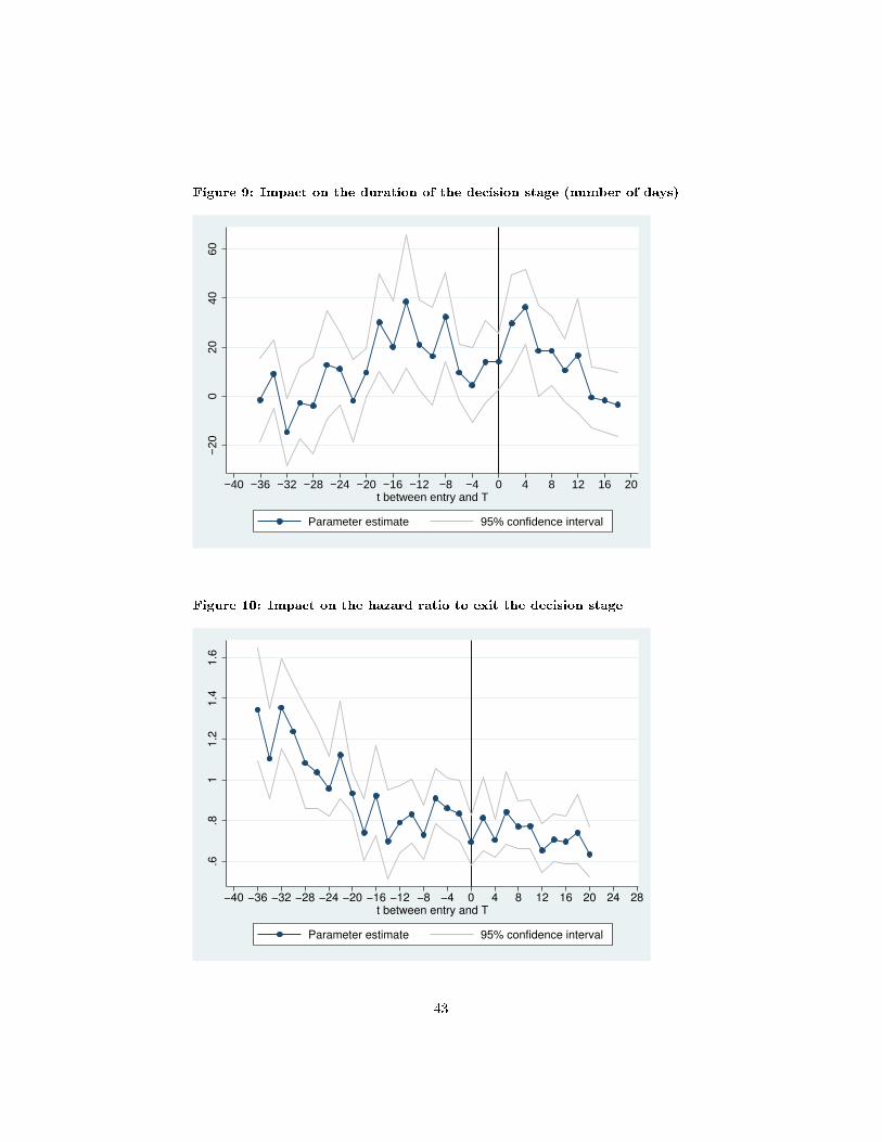
Figure 9: Impact on the duration of the decision stage (number of days)

−20

020

4060

−40 −36 −32 −28 −24 −20 −16 −12 −8 −4 0 4 8 12 16 20t between entry and T

Parameter estimate 95% confidence interval

Figure 10: Impact on the hazard ratio to exit the decision stage

.6.8

11.2

1.4

1.6

−40 −36 −32 −28 −24 −20 −16 −12 −8 −4 0 4 8 12 16 20 24 28t between entry and T

Parameter estimate 95% confidence interval

43

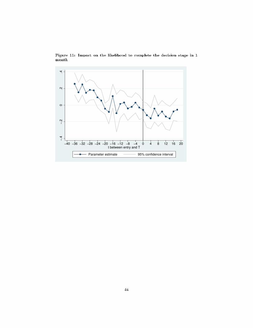
Figure 11: Impact on the likelihood to complete the decision stage in 1month

−.4

−.2

0.2

.4

−40 −36 −32 −28 −24 −20 −16 −12 −8 −4 0 4 8 12 16 20t between entry and T

Parameter estimate 95% confidence interval

44

Figure 12: Impact on the number of pre-trial hearings

−4

−2

02

−40 −36 −32 −28 −24 −20 −16 −12 −8 −4 0 4 8 12 16 20t between entry and T

Parameter estimate 95% confidence interval

Figure 13: Impact on immediate decision likelihood (fast-tracked or inad-missible)

−.2

0.2

.4

−40 −36 −32 −28 −24 −20 −16 −12 −8 −4 0 4 8 12 16 20t between entry and T

Parameter estimate 95% confidence interval

45

Figure 14: Impact on the pre-trial likelihood of being heard

−.1

−.0

50

.05

.1

−40 −36 −32 −28 −24 −20 −16 −12 −8 −4 0 4 8 12 16 20t between entry and T

Parameter estimate 95% confidence interval

Figure 15: Impact on the judge being stricter in the pre-trial

−.1

0.1

.2

−40 −36 −32 −28 −24 −20 −16 −12 −8 −4 0 4 8 12 16 20t between entry and T

Parameter estimate 95% confidence interval

46

Figure 16: Impact on the number of decision stage hearings

−2

−1

01

2

−40 −36 −32 −28 −24 −20 −16 −12 −8 −4 0 4 8 12 16 20t between entry and T

Parameter estimate 95% confidence interval

Figure 17: Impact on the decision stage likelihood of being heard

−.2

−.1

0.1

.2

−40 −36 −32 −28 −24 −20 −16 −12 −8 −4 0 4 8 12 16 20t between entry and T

Parameter estimate 95% confidence interval

47

Figure 18: Impact on the likelihood of pre-trial failure

−.3

−.2

−.1

0.1

−40 −36 −32 −28 −24 −20 −16 −12 −8 −4 0 4 8 12 16 20t between entry and T

Parameter estimate 95% confidence interval

Figure 19: Impact on the likelihood of decision postponement

−.1

0.1

.2

−40 −36 −32 −28 −24 −20 −16 −12 −8 −4 0 4 8 12 16 20t between entry and T

Parameter estimate 95% confidence interval

48

Figure 20: Kaplan-Meier survival estimates

0.0

00.2

50.5

00.7

51.0

0

0 20 40 60t

Before

After

Time of entry

Figure 21: Ongoing cases in pre-trial and decision stages

0

200

400

600

800

1000

1200

1400

Cou

rt−

leve

l: on

goin

g in

pre

−tr

ial a

nd d

ecis

ion

stag

e

1st,3rdcom44 48 52 56 60 64 68 72 76 80 84 92 96 100104108112116

t

Pre−trial Decision stage

49

Figure 22: Di�erential e�ects - pre-trial duration

−20

0−

100

010

020

0

−40 −36 −32 −28 −24 −20 −16 −12 −8 −4 0 4 8 12 16 20t between entry and T

Effect: below medium claim amount 95% confidence intervalEffect: above medium claim amount 95% confidence interval

Figure 23: Number of articles cited

−1.

5−

1−

.50

.5

−40 −36 −32 −28 −24 −20 −16 −12 −8 −4 0 4 8 12 16 20t between entry and T

Parameter estimate 95% confidence interval

50

Figure 24: Relative length of decision

−2

−1

01

2

−40 −36 −32 −28 −24 −20 −16 −12 −8 −4 0 4 8 12 16 20t between entry and T

Parameter estimate 95% confidence interval

Figure 25: Intention to appeal

−.4

−.2

0.2

−40 −36 −32 −28 −24 −20 −16 −12 −8 −4 0 4 8 12 16 20t between entry and T

Parameter estimate 95% confidence interval

51

Figure 26: Relative length of decision

Mean diff= −0.29 P val=0.00

0.5

11.5

Density

0 1 2 3 4 5millions

Pre−reform (5 mos)

Post−reform (3.5 mos)

kernel = epanechnikov, bandwidth = 0.0990

52

Tab

le1:

Su

mm

ary

stati

stic

s-

cham

ber-

level

1st

Com

-m

erci

al

2n

dC

om

-m

erci

al

3rd

Com

-m

erci

al

4th

Com

-m

erci

al

1st

Civ

il2n

dC

ivil

3rd

Civ

il

Ave

rage

nu

mb

er20

12

11.0

13.5

18.7

.13.3

13.7

12.3

ofin

com

ing

case

s20

13

11.5

13.4

12.0

13.2

14.6

4.9

15.7

per

hea

rin

g20

14

21.2

19.2

24.4

9.1

19.0

.23.9

2015

19.5

21.8

26.8

.15.1

.25.8

Ave

rage

nu

mb

er20

12

140.6

188.1

149.1

.22

5.1

165.0

37.0

ofon

goin

gca

ses

2013

116.0

209.1

109.3

63.2

196.2

86.4

89.7

inp

re-t

rial

2014

153.4

201.2

142.0

70.3

156.3

.123.1

2015

174.1

262.1

155.5

.144.8

.134.3

Ave

rage

nu

mb

er20

12

24.7

26.1

46.9

.50.5

48.6

3.0

ofon

goin

gca

ses

2013

26.8

48.7

44.6

16.8

68.6

32.7

31.1

ind

ecis

ion

stag

e20

14

48.7

97.1

84.0

27.0

99.4

.45.9

2015

60.5

107.3

101.4

.85.6

.64.9

i

Tab

le2:

Su

mm

ary

stati

stic

s-

pre

-refo

rmp

eri

od

NM

ean

StD

Med

ian

Min

Max

Du

rati

onof

pre

-tri

alh

eari

ngs

(in

day

s)2827

153.0

34

143.7

53

124.0

00

0.0

00

980.0

00

Lik

elih

ood

ofp

re-t

rial

com

ple

tion

in4

month

s2836

0.4

97

0.5

00

0.0

00

0.0

00

1.0

00

Du

rati

onof

dec

isio

nst

age

(in

day

s)2498

63.9

72

83.3

80

30.0

00

14.0

00

761.0

00

Lik

elih

ood

ofd

ecis

ion

com

ple

tion

in1

month

2529

0.4

94

0.5

00

0.0

00

0.0

00

1.0

00

Nu

mb

erof

pre

tria

lh

eari

ngs

2836

8.0

81

6.4

02

7.0

00

0.0

00

41.0

00

Nu

mb

erof

dec

isio

nst

age

hea

rin

gs

2538

2.6

22

3.4

70

1.0

00

0.0

00

36.0

00

No

pre

-tri

al2836

0.1

21

0.3

26

0.0

00

0.0

00

1.0

00

Pre

-tri

alli

kelih

ood

ofb

ein

gh

eard

2814

0.8

87

0.1

31

0.9

23

0.2

86

1.0

00

Dec

isio

nst

age

like

lih

ood

ofb

ein

gh

eard

2527

0.7

70

0.2

48

0.8

57

0.1

67

1.0

00

Ju

dge

mor

est

rict

2157

0.1

54

0.1

83

0.1

05

0.0

00

1.0

00

Pre

-tri

alin

suffi

cien

t2527

0.1

18

0.3

22

0.0

00

0.0

00

1.0

00

Dec

isio

np

ostp

oned

2527

0.0

55

0.2

29

0.0

00

0.0

00

1.0

00

Cla

imam

ount

(in

1,00

0,00

0F

CFA

)1773

75.6

04

390.2

38

8.0

00

0.0

75

8,7

00.8

38

ii

Tab

le3:

Rob

ust

ness

check

s

(1)

(2)

(3)

(4)

nu

min

nu

min

Ab

ove

med

ian

claim

am

ou

nt

Ab

ove

med

ian

claim

am

ou

nt

Hea

rin

gaft

erd

ecre

e4.9

58

6.1

40

app

lica

tion

(3.0

75)

(4.2

03)

Tre

nd

-0.0

88

-0.0

86

(0.1

04)

(0.1

13)

Inte

ract

ion

0.5

51**

0.4

60

(0.2

55)

(0.2

95)

Ente

red

aft

erd

ecre

e-0

.037

-0.0

38

app

lica

tion

(0.0

41)

(0.0

50)

Tre

nd

0.0

03***

0.0

04***

(0.0

01)

(0.0

01)

Inte

ract

ion

-0.0

05*

-0.0

06*

(0.0

03)

(0.0

03)

Con

stan

t12.7

79**

6.5

72

0.5

26***

0.2

96***

(5.6

95)

(4.9

92)

(0.0

63)

(0.0

61)

Ch

amb

erF

Es

Yes

Yes

Yes

Yes

Cal

end

ar

month

FE

sY

esY

esY

esY

esW

ith

out

ad

j.p

erio

dN

oY

esN

oY

esP

re-m

ean

14.1

90

14.1

90

0.5

01

0.5

01

Pre

-sd

11.5

22

11.5

22

0.5

00

0.5

00

R-S

qu

ared

0.4

03

0.4

33

0.2

01

0.1

93

Ob

serv

ati

on

s310

274

3532

3198

***

p<

0.0

1,

**

p<

0.0

5,

*p<

0.1

.A

llm

od

els

esti

mate

dby

OL

S.

Sta

nd

ard

erro

rsin

pare

nth

eses

,cl

ust

ered

by

cham

ber

-entr

y-t

.W

ind

owin

clu

des

case

sen

teri

ng

bet

wee

n38

hea

rin

gs

bef

ore

an

d20

hea

rin

gs

aft

erd

ecre

eap

plica

-ti

on.

iii

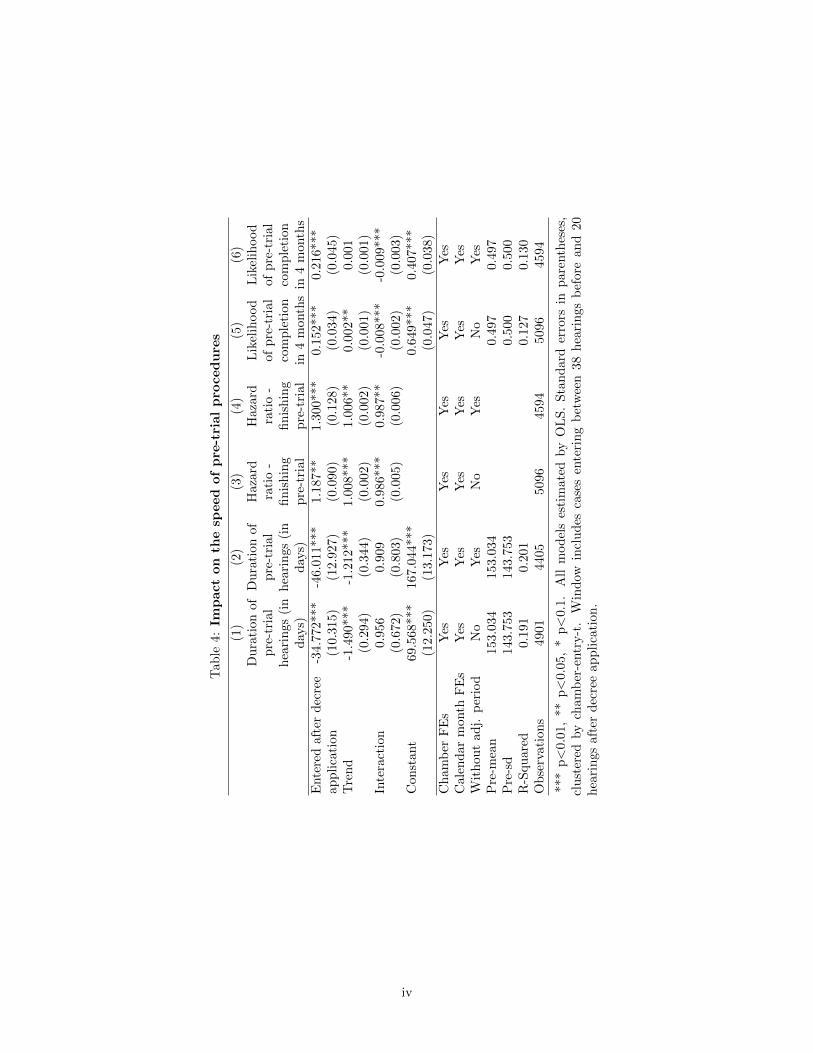
Tab

le4:

Imp

act

on

the

speed

of

pre

-tri

al

pro

ced

ure

s

(1)

(2)

(3)

(4)

(5)

(6)

Du

rati

on

of

pre

-tri

al

hea

rin

gs

(in

day

s)

Du

rati

on

of

pre

-tri

al

hea

rin

gs

(in

day

s)

Haza

rdra

tio

-fi

nis

hin

gp

re-t

rial

Haza

rdra

tio

-fi

nis

hin

gp

re-t

rial

Lik

elih

ood

of

pre

-tri

al

com

ple

tion

in4

month

s

Lik

elih

ood

of

pre

-tri

al

com

ple

tion

in4

month

sE

nte

red

afte

rd

ecre

e-3

4.7

72***

-46.0

11***

1.1

87**

1.3

00***

0.1

52***

0.2

16***

app

lica

tion

(10.3

15)

(12.9

27)

(0.0

90)

(0.1

28)

(0.0

34)

(0.0

45)

Tre

nd

-1.4

90***

-1.2

12***

1.0

08***

1.0

06**

0.0

02**

0.0

01

(0.2

94)

(0.3

44)

(0.0

02)

(0.0

02)

(0.0

01)

(0.0

01)

Inte

ract

ion

0.9

56

0.9

09

0.9

86***

0.9

87**

-0.0

08***

-0.0

09***

(0.6

72)

(0.8

03)

(0.0

05)

(0.0

06)

(0.0

02)

(0.0

03)

Con

stan

t69.5

68***

167.0

44***

0.6

49***

0.4

07***

(12.2

50)

(13.1

73)

(0.0

47)

(0.0

38)

Ch

amb

erF

Es

Yes

Yes

Yes

Yes

Yes

Yes

Cal

end

arm

onth

FE

sY

esY

esY

esY

esY

esY

esW

ith

out

adj.

per

iod

No

Yes

No

Yes

No

Yes

Pre

-mea

n153.0

34

153.0

34

0.4

97

0.4

97

Pre

-sd

143.7

53

143.7

53

0.5

00

0.5

00

R-S

qu

ared

0.1

91

0.2

01

0.1

27

0.1

30

Ob

serv

atio

ns

4901

4405

5096

4594

5096

4594

***

p<

0.01

,**

p<

0.0

5,

*p<

0.1

.A

llm

od

els

esti

mate

dby

OL

S.

Sta

nd

ard

erro

rsin

pare

nth

eses

,cl

ust

ered

by

cham

ber

-entr

y-t

.W

ind

owin

clud

esca

ses

ente

rin

gb

etw

een

38

hea

rin

gs

bef

ore

an

d20

hea

rin

gsaf

ter

dec

ree

ap

pli

cati

on

.

iv

Tab

le5:

Imp

act

on

the

speed

of

the

decis

ion

stage

(1)

(2)

(3)

(4)

(5)

(6)

Du

rati

on

of

dec

isio

nst

age

(in

day

s)

Du

rati

on

of

dec

isio

nst

age

(in

day

s)

Haza

rdra

tio

-fi

nis

hin

gp

re-t

rial

Haza

rdra

tio

-fi

nis

hin

gp

re-t

rial

Lik

elih

ood

of

dec

isio

nco

mp

leti

on

in1

month

Lik

elih

ood

of

dec

isio

nco

mp

leti

on

in1

month

Ente

red

afte

rd

ecre

e3.4

26

5.2

17

0.0

79

0.1

64*

-0.0

39

-0.0

09

app

lica

tion

(6.7

78)

(9.2

98)

(0.0

72)

(0.0

88)

(0.0

40)

(0.0

55)

Tre

nd

0.7

06***

0.7

98***

-0.0

14***

-0.0

16***

-0.0

07***

-0.0

08***

(0.1

76)

(0.2

01)

(0.0

02)

(0.0

02)

(0.0

01)

(0.0

01)

Inte

ract

ion

-2.2

03***

-2.6

09***

0.0

03

0.0

01

0.0

06**

0.0

06

(0.4

22)

(0.5

99)

(0.0

05)

(0.0

06)

(0.0

03)

(0.0

03)

Con

stan

t104.0

72***

65.7

08***

0.4

40***

0.4

74***

(8.5

65)

(8.1

04)

(0.0

77)

(0.0

71)

Ch

amb

erF

Es

Yes

Yes

Yes

Yes

Yes

Yes

Cal

end

arm

onth

FE

sY

esY

esY

esY

esY

esY

esW

ith

out

adj.

per

iod

No

Yes

No

Yes

No

Yes

Pre

-mea

n63.9

72

63.9

72

0.4

94

0.4

94

Pre

-sd

83.3

80

83.3

80

0.5

00

0.5

00

R-S

qu

ared

0.0

61

0.0

64

0.1

55

0.1

54

Ob

serv

atio

ns

3851

3496

4109

3738

4116

3745

***

p<

0.01

,**

p<

0.0

5,

*p<

0.1

.A

llm

od

els

esti

mate

dby

OL

S.

Sta

nd

ard

erro

rsin

pare

nth

eses

,cl

ust

ered

by

cham

ber

-entr

y-t

.W

ind

owin

clud

esca

ses

ente

rin

gb

etw

een

38

hea

rin

gs

bef

ore

an

d20

hea

rin

gsaf

ter

dec

ree

ap

pli

cati

on

.

v

Tab

le6:

Imp

act

on

the

pre

-tri

al

stage:

Ch

an

nels

(1)

(2)

(3)

(4)

(5)

(6)

(7)

(8)

Nu

mb

erof

pre

tria

lh

eari

ngs

Nu

mb

erof

pre

tria

lh

eari

ngs

No

pre

-tri

al

No

pre

-tri

al

Pre

-tri

al

like

lih

ood

of

bei

ng

hea

rd

Pre

-tri

al

like

lih

ood

of

bei

ng

hea

rd

Ju

dge

more

stri

ctJu

dge

more

stri

ct

Ente

red

afte

rd

ecre

e-1

.423

***

-1.9

13***

0.1

83***

0.2

38***

0.0

51***

0.0

62***

0.0

55***

0.0

62***

app

lica

tion

(0.4

19)

(0.5

20)

(0.0

30)

(0.0

38)

(0.0

12)

(0.0

18)

(0.0

15)

(0.0

23)

Tre

nd

-0.0

59**

*-0

.043***

0.0

03***

0.0

02**

-0.0

00

-0.0

01

-0.0

01**

-0.0

01**

(0.0

13)

(0.0

15)

(0.0

01)

(0.0

01)

(0.0

00)

(0.0

00)

(0.0

00)

(0.0

01)

Inte

ract

ion

0.07

8***

0.0

65*

-0.0

08***

-0.0

08***

0.0

01

0.0

00

0.0

05***

0.0

05***

(0.0

28)

(0.0

35)

(0.0

02)

(0.0

03)

(0.0

01)

(0.0

01)

(0.0

01)

(0.0

02)

Con

stan

t7.

322*

**5.5

48***

0.1

37***

0.2

10***

0.8

59***

0.7

80***

0.1

59***

0.1

39***

(0.4

11)

(0.5

71)

(0.0

33)

(0.0

37)

(0.0

14)

(0.0

16)

(0.0

16)

(0.0

18)

Ch

amb

erF

Es

Yes

Yes

Yes

Yes

Yes

Yes

Yes

Yes

Cal

end

arm

onth

FE

sY

esY

esY

esY

esY

esY

esY

esY

esW

ith

out

adj.

per

iod

No

Yes

No

Yes

No

Yes

No

Yes

Pre

-mea

n8.

057

8.0

57

0.1

20

0.1

20

0.8

87

0.8

87

0.1

54

0.1

54

Pre

-sd

6.41

76.4

17

0.3

25

0.3

25

0.1

31

0.1

31

0.1

82

0.1

82

R-S

qu

ared

0.13

50.1

42

0.0

96

0.1

04

0.2

06

0.2

17

0.0

67

0.0

69

Ob

serv

atio

ns

5169

4667

5169

4667

5137

4638

3434

3141

***

p<

0.01

,**

p<

0.05

,*

p<

0.1.

All

mod

els

esti

mate

dby

OL

S.

Sta

nd

ard

erro

rsin

pare

nth

eses

,cl

ust

ered

by

cham

ber

-entr

y-t

.W

ind

owin

clu

des

case

sen

teri

ng

bet

wee

n38

hea

rin

gs

bef

ore

an

d20

hea

rin

gs

aft

erd

ecre

eap

pli

cati

on

.

vi

Tab

le7:

Imp

act

on

the

decis

ion

stage:

Ch

an

nels

(1)

(2)

(3)

(4)

Nu

mb

erof

dec

isio

nst

age

hea

rin

gs

Nu

mb

erof

dec

isio

nst

age

hea

rin

gs

Dec

isio

nst

age

like

lih

ood

of

bei

ng

hea

rd

Dec

isio

nst

age

like

lih

ood

of

bei

ng

hea

rdE

nte

red

aft

erd

ecre

e-0

.087

0.0

12

0.0

22

0.0

46

app

lica

tion

(0.2

96)

(0.3

79)

(0.0

26)

(0.0

39)

Tre

nd

0.0

20***

0.0

22***

-0.0

05***

-0.0

06***

(0.0

07)

(0.0

08)

(0.0

01)

(0.0

01)

Inte

ract

ion

-0.0

79***

-0.0

89***

0.0

06***

0.0

07**

(0.0

19)

(0.0

25)

(0.0

02)

(0.0

03)

Con

stan

t2.9

98***

2.4

14***

0.7

69***

0.7

91***

(0.3

26)

(0.3

40)

(0.0

24)

(0.0

30)

Ch

amb

erF

Es

Yes

Yes

Yes

Yes

Cal

end

ar

month

FE

sY

esY

esY

esY

esW

ith

out

ad

j.p

erio

dN

oY

esN

oY

esP

re-m

ean

2.6

15

2.6

15

0.7

73

0.7

73

Pre

-sd

3.4

42

3.4

42

0.2

47

0.2

47

R-S

qu

ared

0.0

29

0.0

30

0.3

07

0.2

98

Ob

serv

ati

on

s4377

4000

4137

3768

***

p<

0.0

1,

**

p<

0.0

5,

*p<

0.1

.A

llm

od

els

esti

mate

dby

OL

S.

Sta

nd

ard

erro

rsin

pare

nth

eses

,cl

ust

ered

by

cham

ber

-entr

y-t

.W

ind

owin

clu

des

case

sen

teri

ng

bet

wee

n38

hea

rin

gs

bef

ore

an

d20

hea

rin

gs

aft

erd

ecre

eap

plica

-ti

on.

vii

Tab

le8:

Imp

act

on

pre

-tri

al

qu

ali

ty

(1)

(2)

(3)

(4)

Pre

-tri

al

insu

ffici

ent

Pre

-tri

al

insu

ffici

ent

Dec

isio

np

ost

poned

Dec

isio

np

ost

pon

edE

nte

red

aft

erd

ecre

e0.0

26

0.0

17

-0.0

09

-0.0

04

app

lica

tion

(0.0

29)

(0.0

42)

(0.0

22)

(0.0

29)

Tre

nd

0.0

01**

0.0

01

0.0

01***

0.0

02***

(0.0

01)

(0.0

01)

(0.0

01)

(0.0

01)

Inte

ract

ion

0.0

01

0.0

03

-0.0

01

-0.0

02

(0.0

02)

(0.0

03)

(0.0

02)

(0.0

02)

Con

stan

t0.0

98***

0.1

66***

0.0

19

0.0

56***

(0.0

33)

(0.0

40)

(0.0

17)

(0.0

21)

Ch

amb

erF

Es

Yes

Yes

Yes

Yes

Cal

end

ar

month

FE

sY

esY

esY

esY

esW

ith

out

ad

j.p

erio

dN

oY

esN

oY

esP

re-m

ean

0.1

20

0.1

20

0.0

54

0.0

54

Pre

-sd

0.3

25

0.3

25

0.2

27

0.2

27

R-S

qu

ared

0.0

18

0.0

20

0.0

43

0.0

45

Ob

serv

ati

on

s4137

3768

4137

3768

***

p<

0.0

1,

**

p<

0.0

5,

*p<

0.1

.A

llm

od

els

esti

mate

dby

OL

S.

Sta

nd

ard

erro

rsin

pare

nth

eses

,cl

ust

ered

by

cham

ber

-entr

y-t

.W

ind

owin

clu

des

case

sen

teri

ng

bet

wee

n38

hea

rin

gs

bef

ore

an

d20

hea

rin

gs

aft

erd

ecre

eap

plica

-ti

on.

viii

Tab

le9:

Imp

act

on

decis

ion

qu

ali

ty

(1)

(2)

(3)

(4)

(5)

(6)

Nu

mb

erof

art

icle

sN

um

ber

of

art

icle

sD

ecis

ion

len

gth

Dec

isio

nle

ngth

Ap

pea

lA

pp

eal

Ente

red

afte

rd

ecre

e0.0

52

-0.1

42

0.0

71

-0.1

60

0.0

65

0.0

51

app

lica

tion

(0.1

20)

(0.1

69)

(0.1

84)

(0.2

28)

(0.0

47)

(0.0

55)

Tre

nd

-0.0

00

0.0

02

-0.0

04

-0.0

03

0.0

00

0.0

00

(0.0

04)

(0.0

04)

(0.0

06)

(0.0

06)

(0.0

01)

(0.0

01)

Inte

ract

ion

0.0

00

0.0

09

0.0

14

0.0

29*

-0.0

01

-0.0

01

(0.0

09)

(0.0

12)

(0.0

14)

(0.0

16)

(0.0

03)

(0.0

04)

Con

stan

t2.9

46***

2.8

83***

6.3

49***

5.3

06***

0.5

88***

0.5

93***

(0.2

03)

(0.2

39)

(0.2

45)

(0.2

00)

(0.0

59)

(0.0

68)

Ch

amb

erF

Es

Yes

Yes

Yes

Yes

Yes

Yes

Cal

end

arm

onth

FE

sY

esY

esY

esY

esY

esY

esW

ith

out

adj.

per

iod

No

Yes

No

Yes

No

Yes

Pre

-mea

n2.8

35

2.8

46

5.5

33

5.5

47

0.5

35

0.5

37

Pre

-sd

1.5

65

1.5

95

2.5

20

2.5

68

0.4

99

0.4

99

R-S

qu

ared

0.0

07

0.0

05

0.0

35

0.0

38

0.0

37

0.0

40

Ob

serv

atio

ns

2985

2672

2984

2671

2985

2672

***

p<

0.01

,**

p<

0.0

5,

*p<

0.1

.A

llm

od

els

esti

mate

dby

OL

S.

Sta

nd

ard

erro

rsin

pare

nth

eses

,cl

ust

ered

by

cham

ber

-entr

y-t

.W

ind

owin

clud

esca

ses

ente

rin

gb

etw

een

38

hea

rin

gs

bef

ore

an

d20

hea

rin

gsaf

ter

dec

ree

ap

pli

cati

on

.

ix

Tab

le10:

Diff

ere

nti

al

imp

acts

by

case

diffi

cu

lty:

cla

imam

ou

nt

(1)

(2)

(3)

(4)

(5)

(6)

(7)

Du

rati

on

of

pre

-tri

al

hea

rin

gs

(in

day

s)

Lik

elih

ood

of

pre

-tri

al

com

ple

tion

in4

month

s

Nu

mb

erof

pre

tria

lh

eari

ngs

Pre

-tri

al

like

lih

ood

of

bei

ng

hea

rd

Ju

dge

more

stri

ctP

re-t

rial

insu

ffici

ent

Dec

isio

np

ost

poned

Ab

ove

med

ian

clai

m30.2

52***

-0.1

18***

1.7

04***

-0.0

05

-0.0

06

0.0

62*

0.0

89***

amou

nt

(10.0

89)

(0.0

39)

(0.4

73)

(0.0

12)

(0.0

23)

(0.0

34)

(0.0

23)

Ente

red

afte

rd

ecre

e-2

6.5

38**

0.1

07**

-1.1

36*

0.0

39***

0.0

42

-0.0

34

-0.0

07

app

lica

tion

(13.4

80)

(0.0

52)

(0.6

33)

(0.0

14)

(0.0

29)

(0.0

40)

(0.0

27)

Ab

mcl

aim

amou

nt

X-1

.824

-0.0

11

-0.1

87

-0.0

10

0.0

61*

0.0

96*

-0.0

47

Ente

red

afte

r(1

5.9

04)

(0.0

60)

(0.7

32)

(0.0

15)

(0.0

33)

(0.0

54)

(0.0

40)

Tre

nd

-0.0

63

-0.0

01

-0.0

10

-0.0

01**

-0.0

01

0.0

00

0.0

01*

(0.4

25)

(0.0

02)

(0.0

20)

(0.0

00)

(0.0

01)

(0.0

01)

(0.0

01)

Ente

red

afte

rd

ecre

e-1

.065

0.0

01

-0.0

06

0.0

02**

0.0

07***

0.0

09***

0.0

02

app

lica

tion

XT

ren

d(0

.845)

(0.0

03)

(0.0

39)

(0.0

01)

(0.0

02)

(0.0

03)

(0.0

02)

Ab

mcl

aim

amou

nt

X-1

.525***

0.0

03

-0.0

49**

0.0

01

-0.0

00

0.0

02

0.0

02***

Tre

nd

(0.5

24)

(0.0

02)

(0.0

24)

(0.0

00)

(0.0

01)

(0.0

02)

(0.0

01)

Tri

ple

inte

ract

ion

0.4

26

-0.0

03

0.0

23

-0.0

01

-0.0

03

-0.0

12***

-0.0

06**

(1.1

34)

(0.0

04)

(0.0

48)

(0.0

01)

(0.0

02)

(0.0

04)

(0.0

03)

Con

stan

t79.0

05***

0.3

36***

7.7

29***

0.7

86***

0.1

48***

0.1

35***

0.0

50

(14.4

21)

(0.0

47)

(0.6

30)

(0.0

18)

(0.0

24)

(0.0

48)

(0.0

31)

Eff

ect

for

larg

eca

ses

-28.3

62

.096

-1.3

23

.029

.103

.062

-.053

P-v

alu

e:eff

ect

for

larg

eca

ses

.0285

.0488

.02

.0437

0.2

072

.1282

Ch

amb

erF

Es

Yes

Yes

Yes

Yes

Yes

Yes

Yes

Cal

end

arm

onth

FE

sY

esY

esY

esY

esY

esY

esY

esW

ith

out

adju

stm

ent

per

iod

No

No

No

No

No

No

No

Pre

-mea

n100.0

71

0.6

69

5.8

78

0.9

27

0.1

49

0.0

93

0.0

24

Pre

-sd

117.0

08

0.4

71

5.3

38

0.1

17

0.1

89

0.2

91

0.1

53

R-S

qu

ared

0.2

24

0.1

53

0.1

77

0.2

21

0.0

90

0.0

31

0.0

53

Ob

serv

atio

ns

3380

3532

3532

3522

2208

2851

2851

***

p<

0.01

,**

p<

0.05

,*

p<

0.1.

All

mod

els

esti

mate

dby

OL

S.

Sta

nd

ard

erro

rsin

pare

nth

eses

,cl

ust

ered

by

cham

ber

-en

try-t

.W

indow

incl

ud

esca

ses

ente

rin

gb

etw

een

38

hea

rin

gs

bef

ore

an

d20

hea

rin

gs

aft

erd

ecre

eap

pli

cati

on

.

x

Tab

le11

:D

iffere

nti

al

imp

acts

by

case

diffi

cu

lty:

cla

imam

ou

nt

(wit

hou

tad

just

ment

peri

od

)

(1)

(2)

(3)

(4)

(5)

(6)

(7)

Du

rati

on

of

pre

-tri

al

hea

rin

gs

(in

day

s)

Lik

elih

ood

of

pre

-tri

al

com

ple

tion

in4

month

s

Nu

mb

erof

pre

tria

lh

eari

ngs

Pre

-tri

al

like

lih

ood

of

bei

ng

hea

rd

Ju

dge

more

stri

ctP

re-t

rial

insu

ffici

ent

Dec

isio

np

ost

poned

Ab

ove

med

ian

clai

m27.5

30**

-0.0

89*

1.4

77**

-0.0

08

-0.0

30

0.0

97**

0.1

03***

amou

nt

(13.1

21)

(0.0

52)

(0.6

12)

(0.0

13)

(0.0

26)

(0.0

40)

(0.0

28)

Ente

red

afte

rd

ecre

e-5

5.7

98***

0.2

29***

-2.6

78***

0.0

49***

-0.0

02

-0.0

21

0.0

05

app

lica

tion

(17.1

59)

(0.0

65)

(0.7

94)

(0.0

19)

(0.0

43)

(0.0

54)

(0.0

37)

Ab

mcl

aim

amou

nt

X26.6

78

-0.1

16

1.4

05

-0.0

11

0.1

23***

0.0

73

-0.0

46

Ente

red

afte

r(1

9.7

81)

(0.0

76)

(0.9

16)

(0.0

18)

(0.0

45)

(0.0

70)

(0.0

57)

Tre

nd

0.3

04

-0.0

02

0.0

11

-0.0

01*

-0.0

01

-0.0

00

0.0

01

(0.5

15)

(0.0

02)

(0.0

24)

(0.0

01)

(0.0

01)

(0.0

01)

(0.0

01)

Ente

red

afte

rd

ecre

e-0

.082

-0.0

04

0.0

42

0.0

01

0.0

09***

0.0

10**

0.0

02

app

lica

tion

XT

ren

d(0

.961)

(0.0

04)

(0.0

45)

(0.0

01)

(0.0

03)

(0.0

04)

(0.0

03)

Ab

mcl

aim

amou

nt

X-1

.596**

0.0

04*

-0.0

57**

0.0

01

-0.0

01

0.0

03*

0.0

03***

Tre

nd

(0.6

18)

(0.0

02)

(0.0

28)

(0.0

01)

(0.0

01)

(0.0

02)

(0.0

01)

Tri

ple

inte

ract

ion

-1.3

97

0.0

02

-0.0

68

-0.0

00

-0.0

05*

-0.0

14**

-0.0

08*

(1.3

30)

(0.0

05)

(0.0

56)

(0.0

01)

(0.0

03)

(0.0

05)

(0.0

04)

Con

stan

t178.3

99***

0.6

27***

5.0

80***

0.7

88***

0.1

33***

0.1

02*

0.0

03

(18.3

61)

(0.0

63)

(0.7

91)

(0.0

22)

(0.0

25)

(0.0

59)

(0.0

22)

Eff

ect

for

larg

eca

ses

-29.1

2.1

13

-1.2

73

.038

.121

.052

-.041

P-v

alu

e:eff

ect

for

larg

eca

ses

.0735

.0771

.0797

.0439

.0001

.42

.3738

Ch

amb

erF

Es

Yes

Yes

Yes

Yes

Yes

Yes

Yes

Cal

end

arm

onth

FE

sY

esY

esY

esY

esY

esY

esY

esW

ith

out

adju

stm

ent

per

iod

Yes

Yes

Yes

Yes

Yes

Yes

Yes

Pre

-mea

n100.0

71

0.6

69

5.8

78

0.9

27

0.1

49

0.0

93

0.0

24

Pre

-sd

117.0

08

0.4

71

5.3

38

0.1

17

0.1

89

0.2

91

0.1

53

R-S

qu

ared

0.2

33

0.1

51

0.1

83

0.2

25

0.0

96

0.0

32

0.0

57

Ob

serv

atio

ns

3051

3198

3198

3188

2019

2596

2596

***

p<

0.01

,**

p<

0.05

,*

p<

0.1.

All

mod

els

esti

mate

dby

OL

S.

Sta

nd

ard

erro

rsin

pare

nth

eses

,cl

ust

ered

by

cham

ber

-en

try-t

.W

indow

incl

ud

esca

ses

ente

rin

gb

etw

een

38

hea

rin

gs

bef

ore

an

d20

hea

rin

gs

aft

erd

ecre

eap

pli

cati

on

.

xi

Tab

le12:

Perc

ep

tion

s

(1)

(2)

(3)

(4)

(5)

(6)

(7)

(8)

Du

rati

onD

ura

tion

Cost

Cost

Hyp

oth

.1

Hyp

oth

.1

Ind

ex1

Ind

ex1

Tre

at3.

937*

3.7

58

455.3

96*

433.4

53*

0.0

47

0.042

0.0

63*

0.0

63*

(2.2

93)

(2.3

25)

(246.4

65)

(249.4

74)

(0.0

57)

(0.0

58)

(0.0

34)

(0.0

34)

BL

nu

mb

erof

-0.0

00-0

.001

1.7

98***

1.6

72***

0.0

00

0.000

0.0

00

0.0

00

emp

loye

es(0

.004

)(0

.004)

(0.3

94)

(0.4

16)

(0.0

00)

(0.0

00)

(0.0

00)

(0.0

00)

Res

p.:

jur

2.1

02

390.1

17

0.032

-0.0

43

(3.9

35)

(426.2

33)

(0.0

96)

(0.0

58)

Res

p.:

oth

0.6

92

-57.8

73

0.036

0.0

55

(2.4

26)

(260.7

59)

(0.0

61)

(0.0

36)

Con

stan

t20

.552

***

20.1

70***

992.9

47***

993.4

45***

0.7

67***

0.7

52***

0.4

91***

0.4

72***

(1.7

01)

(1.9

95)

(182.6

74)

(211.7

93)

(0.0

42)

(0.0

49)

(0.0

25)

(0.0

29)

Pre

-mea

n20

.591

20.5

91

976.4

21

976.4

21

0.7

79

0.7

79

0.5

03

0.5

03

R-S

qu

ared

0.01

30.0

15

0.1

11

0.1

16

0.0

08

0.0

10

0.0

17

0.0

35

Ob

serv

atio

ns

223

223

220

220

204

204

226

226

***

p<

0.01

,**

p<

0.05

,*

p<

0.1

.A

llm

od

els

esti

mate

dby

OL

S.

Sta

nd

ard

erro

rsin

pare

nth

eses

.

xii

Tab

le13:

Fir

m-l

evel

(1)

(2)

(3)

(4)

(5)

(6)

Nu

mb

erof

emp

loye

esN

um

ber

of

emp

loye

esP

ub

lic

len

der

Pu

bli

cle

nd

erO

ngoin

glo

an

On

goin

glo

an

Tre

at19.5

60*

15.0

03

0.1

20**

0.1

17*

0.1

93***

0.1

53**

(11.0

21)

(11.0

08)

(0.0

59)

(0.0

59)

(0.0

64)

(0.0

62)

BL

num

ber

of

0.3

11***

0.2

97***

0.0

00

0.0

00

0.0

00*

0.0

00

emp

loye

es(0

.018)

(0.0

19)

(0.0

00)

(0.0

00)

(0.0

00)

(0.0

00)

Res

p.:

jur

49.5

52***

-0.0

06

0.4

32***

(18.7

26)

(0.1

01)

(0.1

05)

Res

p.:

oth

18.2

36

0.0

67

0.1

74***

(11.4

89)

(0.0

62)

(0.0

65)

Con

stan

t23.8

72***

14.3

39

0.1

80***

0.1

55***

0.2

45***

0.1

56***

(8.1

61)

(9.3

70)

(0.0

44)

(0.0

50)

(0.0

47)

(0.0

53)

Pre

-mea

n30.2

48

30.2

48

0.1

74

0.1

74

0.2

45

0.2

45

R-S

qu

ared

0.5

90

0.6

04

0.0

25

0.0

31

0.062

0.1

36

Ob

serv

atio

ns

226

226

225

225

226

226

***

p<

0.01

,**

p<

0.0

5,

*p<

0.1

.A

llm

od

els

esti

mate

dby

OL

S.

Sta

nd

ard

erro

rsin

par

enth

eses

.

xiii