energies

Article

Fluid Retrofit for Existing Vapor CompressionRefrigeration Systems and Heat Pumps: Evaluationof Different Models †

Dennis Roskosch *, Valerius Venzik and Burak Atakan

Department of Mechanical and Process Engineering, University of Duisburg-Essen, Thermodynamics,Lotharstr. 1, 47057 Duisburg, Germany; valerius.venzik@uni-due.de (V.V.); burak.atakan@uni-due.de (B.A.)* Correspondence: dennis.roskosch@uni-due.de† This paper is an extended version of our paper published in 2018 Heat Powered Cycles Conference, Bayreuth,

Germany, 16–19 September 2018; ISBN 978-0-9563329-6-7.

Received: 25 April 2019; Accepted: 20 June 2019; Published: 24 June 2019�����������������

Abstract: The global warming potential of many working fluids used nowadays for vapor compressionrefrigeration systems and heat pumps is very high. Many of such fluids, which are used in currentlyoperating refrigerators and heat pumps, will have to be replaced. In order to avoid a redesign of thesystem, it would be very helpful if efficient and ecological alternative working fluids for a given plantcould be found. With modern process simulation tools such a selection procedure seems possible.However, it remains unclear how detailed such a model of a concrete plant design has to be to obtaina reliable working fluid ranking. A vapor compression heat pump test-rig is used as an exampleand simulated by thermodynamic models with different levels of complexity to investigate thisquestion. Experimental results for numerous working fluids are compared with models of differentcomplexity. Simple cycle calculations, as often used in the literature, lead to incorrect results regardingthe efficiency and are not recommended to find replacement fluids for existing plants. Adding acompressor model improves the simulations significantly and leads to reliable fluid rankings but thisis not sufficient to judge the adequacy of the heat exchanger sizes and whether a given cooling orheating task can be fulfilled with a certain fluid. With a model of highest complexity, including anextensive model for the heat exchangers, this question can also be answered.

Keywords: refrigerants; retrofit; process simulation; replacement fluids; experiments

1. Introduction

As a result of the Montreal Protocol [1], chlorofluorocarbons (CFCs), which previously were usedas working fluids in compression refrigeration cycles and heat pumps, were replaced by substanceswithout ozone depletion potential. Hydrofluorocarbons (HFCs), like R134a, R404A and, R410A, aregood alternatives. They are still used in a wide range of systems today. Some HFCs, although they haveno ozone depletion potential, have an extremely high global warming potential (GWP). They contributesignificantly to global climate change. The United Nations (UN) therefore, decided to reduce theirusage. The resolution of the UN is implemented in the European Union by the F-Gas-Regulation [2]and it includes several different instruments. Direct usage bans apply to refrigerants with a GWPgreater than 2500 (e.g., R404A) and a filling capacity exceeding 40 t CO2 equivalents (according toReference [3]) in the next few years (2020 or 2022). Smaller plants such as those used as householdair conditioning systems or heat pumps are affected by a phase-down scenario. This specifies thatthe quantity of newly produced synthetic refrigerants (measured in CO2 equivalents) placed on theEU market will have to be reduced gradually with reference to the annual quantity between 2009 and

Energies 2019, 12, 2417; doi:10.3390/en12122417 www.mdpi.com/journal/energies

Energies 2019, 12, 2417 2 of 12

2012 to 21% from 2015 to 2030. The second reduction step (to 63%) was enforced at the beginningof 2018. This has already led to a considerable price increase and shortage for some refrigerants(e.g., R134a). This regulation will make it necessary for manufacturers to retrofit, at least, some of theircycles to lower GWP refrigerants. Besides new plants, systems which are already in operation willperhaps have to be modified for further usage; the replacement of the working fluid is then the centralpoint. Industry and academia started research on alternative refrigerants several years ago. Manycriteria are important in the selection process of alternative refrigerants. Environmental aspects ormaterial compatibility are important, but thermodynamic criteria are often crucial for the selectionprocedure. This is the focus of the present work. There are two main approaches in the search foralternative fluids. In the first approach, pure substances or fluid mixtures should have thermodynamicproperties which are similar to the fluids to be substituted. The hydro-fluoro olefins (HFOs) suchas R1234ze(E) or R1234yf, have come into focus [4] in this context. The advantage of this method isthat the selection of a substitute is only based on the refrigerant used so far. These fluids are oftenexpensive and investigations often show lower coefficients of performance (COP) compared to thecurrently used fluids (R1234ze(E) or R1234yf for R134a) [5,6]. In addition, this procedure blocks thepossibility of identifying more efficient working fluids, having differing thermodynamic properties.In such systems, greenhouse gas emissions result from the release of refrigerant due to leakage. Alsoindirectly, the production of the electricity necessary for operation leads to emissions, if the electricityis mainly produced from fossil fuels. Although, the working fluid replacement with lower GWP fluidsis useful, the COP should not be reduced and it would be better if improved. The second approach forfluid selection is based on the plant, and not on the fluid, which was used up to now. This seems tobe more promising. Numerous publications were published in recent years which deal with such anapproach and they often try to identify alternative fluids on a theoretical basis [7–10]. Such studiesfocus mostly on future plants and use very simple theoretical models where heat exchangers oftenare not modeled and compressor efficiencies are assumed to be fluid independent. For new plants,these kinds of studies are well justified because the fluid selection is part of the design process, as theselection of compressors and heat exchangers are. If instead a replacement fluid for a given existingsystem is needed then things change because e.g., it can no longer be assumed that the compressorwill work equally well with any fluid. Similar approaches are seen in experimental studies whichinvestigate the general suitability and efficiency of different fluids in a laboratory scale test-rig [6,11–13]or in single components like compressors or heat exchangers [14–16]. These investigations often leadto interesting heuristics, but they are not very helpful in finding replacement fluids for a concrete plantsince the COP, heat flow rates and compressor power of another concrete system will have with adifferent fluid cannot be estimated. These are important criteria in determining whether a potentialfluid is suitable at all or if other system components must be replaced. Modern process simulationsseem to be most promising in finding individual replacement fluids, regarding the large number ofplant designs. It remains unclear how detailed a concrete plant design must be modeled to obtain areliable ranking of working fluids.

This uncertainty is addressed here. A vapor compression heat pump test-rig is simulated asa function of working fluid with thermodynamic models with three different complexity levels.The simulation results are compared along the different model depth levels and with measured valuesderived from a heat pump test-rig. Here, the fluids R134a, R152a, propane, propene, isobutane anddimethyl ether are investigated theoretically and experimentally at the same operating conditions asthe heat pump. It is hypothetically assumed that R134a is the fluid to be substituted and thus theR134a results are always taken as a reference.

2. Experimental Investigation

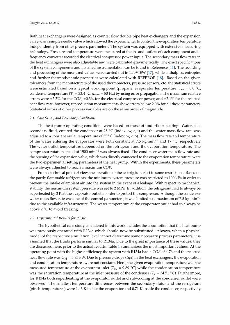
The test-rig was a simple water/water vapor compression heat pump cycle as shown by a simplifiedscheme given in Figure 1. The main components were a semi-hermetic reciprocating compressor (GEABock: HG12P5.4; maximum power (Pmax = 2.2 kW), an expansion valve, a condenser, and an evaporator.

Energies 2019, 12, 2417 3 of 12

Both heat exchangers were designed as counter flow double pipe heat exchangers and the expansionvalve was a simple needle valve which allowed the experimenter to control the evaporation temperatureindependently from other process parameters. The system was equipped with extensive measuringtechnology. Pressure and temperature were measured at the in- and outlets of each component and afrequency converter recorded the electrical compressor power input. The secondary mass flow rates inthe heat exchangers were also adjustable and were calibrated gravimetrically. The exact specificationsof the system components and installed instrumentation can be found in Reference [11]. The recordingand processing of the measured values were carried out in LabVIEW [17], while enthalpies, entropiesand further thermodynamic properties were calculated with REFPROP [18]. Based on the giventolerances from the manufacturers of the used thermometers, pressure sensors, etc. the statistical errorswere estimated based on a typical working point (propane, evaporator temperature (Tev = 0.0 ◦C,condenser temperature (Tc = 33.4 ◦C, ncom = 50 Hz) by using error propagation. The maximum relativeerrors were ±2.2% for the COP, ±0.3% for the electrical compressor power, and ±2.1% for the rejectedheat flow rate, however, reproduction measurements show errors below 2.0% for all these parameters.Statistical errors of other process variables are on the same order of magnitude.

2.1. Case Study and Boundary Conditions

The heat pump operating conditions were based on those of underfloor heating. Water, as asecondary fluid, entered the condenser at 25 ◦C (index: w, c, i) and the water mass flow rate wasadjusted to a constant outlet temperature of 35 ◦C (index: w, c, o). The mass flow rate and temperatureof the water entering the evaporator were both constant at 7.5 kg·min−1 and 17 ◦C, respectively.The water outlet temperature depended on the refrigerant and the evaporation temperature. Thecompressor rotation speed of 1500 min−1 was always fixed. The condenser water mass flow rate andthe opening of the expansion valve, which was directly connected to the evaporation temperature, werethe two experimental setting parameters of the heat pump. Within the experiments, these parameterswere always adjusted to reach a maximum COP.

From a technical point of view, the operation of the test-rig is subject to some restrictions. Based onthe partly flammable refrigerants, the minimum system pressure was restricted to 100 kPa in order toprevent the intake of ambient air into the system in the event of a leakage. With respect to mechanicalstability, the maximum system pressure was set to 2 MPa. In addition, the refrigerant had to always besuperheated by 3 K at the evaporator outlet in order to protect the compressor. Although the condenserwater mass flow rate was one of the control parameters, it was limited to a maximum of 7.5 kg·min−1

due to the available infrastructure. The water temperature at the evaporator outlet had to always beabove 2 ◦C to avoid freezing.

2.2. Experimental Results for R134a

The hypothetical case study considered in this work includes the assumption that the heat pumpwas previously operated with R134a which should now be substituted. Always, when a physicalmodel of the respective simulation level cannot determine some necessary process parameters, it isassumed that the fluids perform similar to R134a. Due to the great importance of these values, theyare discussed here, prior to the actual results. Table 1 summarizes the most important values. At theoperating point with the highest efficiency the system with R134a had a COP of 4.76 and the rejectedheat flow rate was

.QH = 3.85 kW. Due to pressure drops (∆pi) in the heat exchangers, the evaporation

and condensation temperatures were not constant. Here, the given evaporation temperature was themeasured temperature at the evaporator inlet (Tev = 9.89 ◦C) while the condensation temperaturewas the saturation temperature at the inlet pressure of the condenser (Tc = 34.51 ◦C). Furthermore,for R134a both superheating at the evaporator outlet and sub-cooling at the condenser outlet wereobserved. The smallest temperature differences between the secondary fluids and the refrigerant(pinch-temperatures) were 1.43 K inside the evaporator and 0.71 K inside the condenser, respectively.

Energies 2019, 12, 2417 4 of 12

Table 1. Measured data of the reference fluid R134a.

Parameter Value Parameter Value

coefficient of performance, COP 4.76 pinch-temperature evaporator, ∆TPinch,ev 1.43 Krejected heat flow rate,

.QH 3.85 kW condensation temperature, Tc 34.51 ◦C

electrical compressor power, Pcom 0.81 kW sub-cooling condenser outlet, ∆Tsubcooling 2.11 Kevaporation temperature, Tev 9.89 ◦C pressure loss condenser, ∆pc 21.56 kPa

compressor inlet temperature, T1 14.89 ◦C pinch-temperature condenser, ∆TPinch,c 0.71 Kpressure loss evaporator, ∆pev 64.65 kPa isentropic compressor efficiency, ηs

com 0.47

Energies 2019, 12, x FOR PEER REVIEW 4 of 12

these values, they are discussed here, prior to the actual results. Table 1 summarizes the most important values. At the operating point with the highest efficiency the system with R134a had a COP of 4.76 and the rejected heat flow rate was

HQ = 3.85 kW. Due to pressure drops (Δpi) in the heat exchangers, the evaporation and condensation temperatures were not constant. Here, the given evaporation temperature was the measured temperature at the evaporator inlet (Tev = 9.89 °C) while the condensation temperature was the saturation temperature at the inlet pressure of the condenser (Tc = 34.51 °C). Furthermore, for R134a both superheating at the evaporator outlet and sub-cooling at the condenser outlet were observed. The smallest temperature differences between the secondary fluids and the refrigerant (pinch-temperatures) were 1.43 K inside the evaporator and 0.71 K inside the condenser, respectively.

Compressor

Condenser

Evaporator

Throttle

4 1

23

w,e,iw,e,o

w,c,i w,c,o

Figure 1. Heat pump scheme of the simulation models and the experiment.

3. Modeling

All simulation programs were written in the programming language Python [19] and the fluid properties were taken from the database REFPROP [18]. At simulation level II, a numerical optimizer non-linear problem (NLP) was used, taken from the OpenOpt network [20]. The simulations were based on the process scheme given in Figure 1 and the state numbers in the following were referenced to those given in Figure 1. For all simulation levels, an isenthalpic expansion in the throttle was assumed and the heat exchangers were considered to be adiabatic against the environment. The conditions and restrictions of the test-rig were set as described and applied similarly in all simulations.

3.1. Simulation Level I

Simulation level I included only a simple thermodynamic cycle calculation with specific values and largely ideal conditions. Constant isentropic compressor efficiencies were used for all fluids and heat exchanger pressure losses were neglected as is frequently used for fluid selection by other authors [7,8]. Since no physical models were implemented for the different components, numerous cycle states had to be specified. These included the evaporation temperature Tev, the condensation temperature Tc, the compressor inlet temperature T1, the sub-cooling ΔTsubcooling at the condenser outlet, and the isentropic compressor efficiency s

comη . Simulation level I did not capture the differences in operating conditions when different fluids were used in a concrete system. Here, the simplest and obvious assumption was that all components, such as heat exchangers and the compressor, operated similarly with different fluids. Thus, the required process variables were set here to the values which were measured with the reference fluid R134a (Table 1).

Figure 1. Heat pump scheme of the simulation models and the experiment.

3. Modeling

All simulation programs were written in the programming language Python [19] and the fluidproperties were taken from the database REFPROP [18]. At simulation level II, a numerical optimizernon-linear problem (NLP) was used, taken from the OpenOpt network [20]. The simulations werebased on the process scheme given in Figure 1 and the state numbers in the following were referenced tothose given in Figure 1. For all simulation levels, an isenthalpic expansion in the throttle was assumedand the heat exchangers were considered to be adiabatic against the environment. The conditions andrestrictions of the test-rig were set as described and applied similarly in all simulations.

3.1. Simulation Level I

Simulation level I included only a simple thermodynamic cycle calculation with specific valuesand largely ideal conditions. Constant isentropic compressor efficiencies were used for all fluidsand heat exchanger pressure losses were neglected as is frequently used for fluid selection by otherauthors [7,8]. Since no physical models were implemented for the different components, numerouscycle states had to be specified. These included the evaporation temperature Tev, the condensationtemperature Tc, the compressor inlet temperature T1, the sub-cooling ∆Tsubcooling at the condenseroutlet, and the isentropic compressor efficiency ηs

com. Simulation level I did not capture the differencesin operating conditions when different fluids were used in a concrete system. Here, the simplest andobvious assumption was that all components, such as heat exchangers and the compressor, operatedsimilarly with different fluids. Thus, the required process variables were set here to the values whichwere measured with the reference fluid R134a (Table 1).

3.2. Simulation Level II

The second level was based on simulation level I but was significantly expanded by implementinga compressor model. The compressor model used was a semi-physical model which predictedvolumetric and isentropic efficiencies as a function of the inlet state, the outlet pressure, and theworking fluid. It was easily fitted to a concrete reciprocating compressor. It is already described in

Energies 2019, 12, 2417 5 of 12

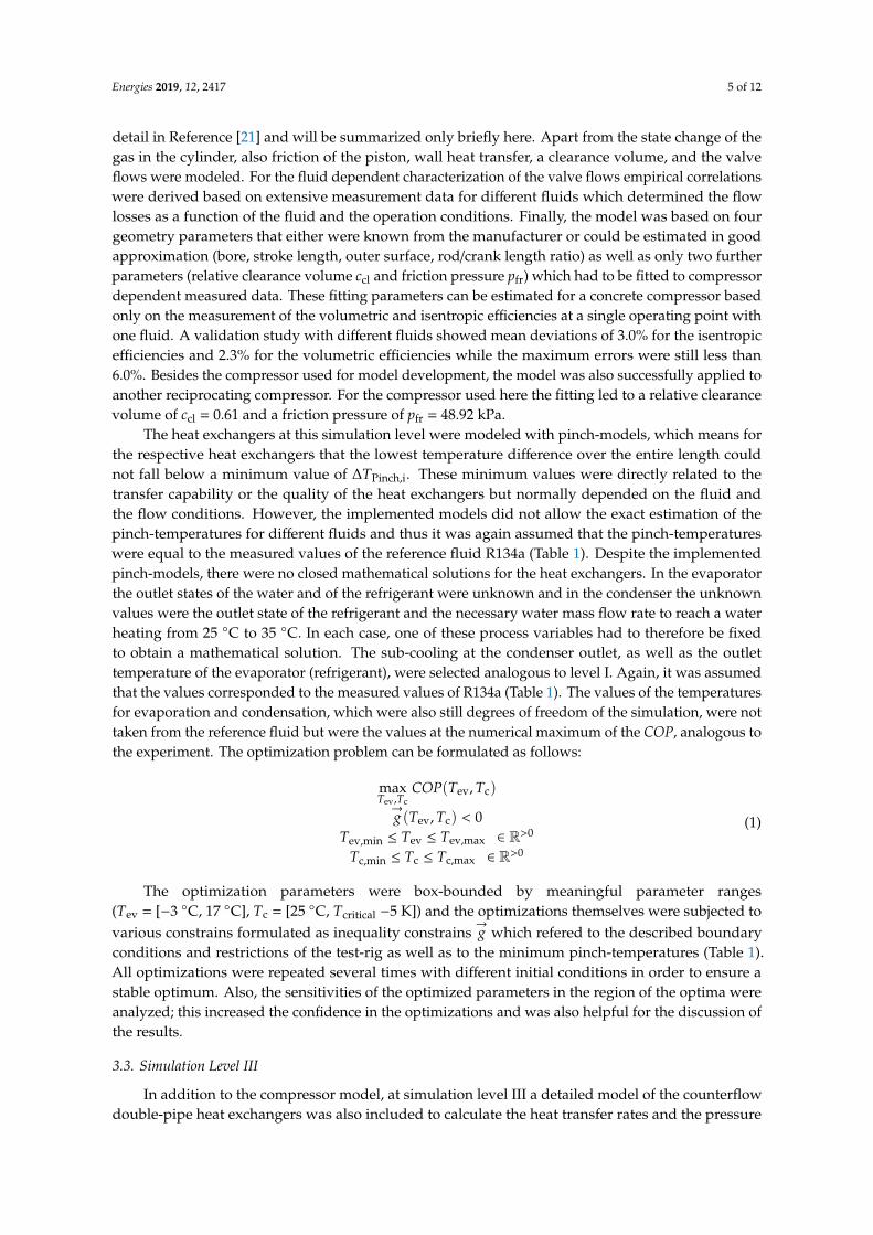
detail in Reference [21] and will be summarized only briefly here. Apart from the state change of thegas in the cylinder, also friction of the piston, wall heat transfer, a clearance volume, and the valveflows were modeled. For the fluid dependent characterization of the valve flows empirical correlationswere derived based on extensive measurement data for different fluids which determined the flowlosses as a function of the fluid and the operation conditions. Finally, the model was based on fourgeometry parameters that either were known from the manufacturer or could be estimated in goodapproximation (bore, stroke length, outer surface, rod/crank length ratio) as well as only two furtherparameters (relative clearance volume ccl and friction pressure pfr) which had to be fitted to compressordependent measured data. These fitting parameters can be estimated for a concrete compressor basedonly on the measurement of the volumetric and isentropic efficiencies at a single operating point withone fluid. A validation study with different fluids showed mean deviations of 3.0% for the isentropicefficiencies and 2.3% for the volumetric efficiencies while the maximum errors were still less than6.0%. Besides the compressor used for model development, the model was also successfully applied toanother reciprocating compressor. For the compressor used here the fitting led to a relative clearancevolume of ccl = 0.61 and a friction pressure of pfr = 48.92 kPa.

The heat exchangers at this simulation level were modeled with pinch-models, which means forthe respective heat exchangers that the lowest temperature difference over the entire length couldnot fall below a minimum value of ∆TPinch,i. These minimum values were directly related to thetransfer capability or the quality of the heat exchangers but normally depended on the fluid andthe flow conditions. However, the implemented models did not allow the exact estimation of thepinch-temperatures for different fluids and thus it was again assumed that the pinch-temperatureswere equal to the measured values of the reference fluid R134a (Table 1). Despite the implementedpinch-models, there were no closed mathematical solutions for the heat exchangers. In the evaporatorthe outlet states of the water and of the refrigerant were unknown and in the condenser the unknownvalues were the outlet state of the refrigerant and the necessary water mass flow rate to reach a waterheating from 25 ◦C to 35 ◦C. In each case, one of these process variables had to therefore be fixedto obtain a mathematical solution. The sub-cooling at the condenser outlet, as well as the outlettemperature of the evaporator (refrigerant), were selected analogous to level I. Again, it was assumedthat the values corresponded to the measured values of R134a (Table 1). The values of the temperaturesfor evaporation and condensation, which were also still degrees of freedom of the simulation, were nottaken from the reference fluid but were the values at the numerical maximum of the COP, analogous tothe experiment. The optimization problem can be formulated as follows:

maxTev,Tc

COP(Tev, Tc)

→g (Tev, Tc) < 0

Tev,min ≤ Tev ≤ Tev,max ∈ R>0

Tc,min ≤ Tc ≤ Tc,max ∈ R>0

(1)

The optimization parameters were box-bounded by meaningful parameter ranges(Tev = [−3 ◦C, 17 ◦C], Tc = [25 ◦C, Tcritical −5 K]) and the optimizations themselves were subjected tovarious constrains formulated as inequality constrains

→g which refered to the described boundary

conditions and restrictions of the test-rig as well as to the minimum pinch-temperatures (Table 1).All optimizations were repeated several times with different initial conditions in order to ensure astable optimum. Also, the sensitivities of the optimized parameters in the region of the optima wereanalyzed; this increased the confidence in the optimizations and was also helpful for the discussion ofthe results.

3.3. Simulation Level III

In addition to the compressor model, at simulation level III a detailed model of the counterflowdouble-pipe heat exchangers was also included to calculate the heat transfer rates and the pressure

Energies 2019, 12, 2417 6 of 12

drops for the fluids. The heat-exchanger model was based on the cell method [22]. The heat transferbetween the refrigerant and the secondary fluid took place along a series of two convective heat transfersteps and the heat conduction through the inner pipe wall. According to the different sections, whereevaporation, condensation or superheating took place, different correlations for heat transfer andpressure drop were implemented, as given in Table 2. These correlations were, in a pre-selection study,found to be particularly suitable. The heat exchanger model indeed significantly expanded the entiremodel, but the evaporation and the condensation temperatures were still degrees of freedom of thesimulation. The test-rig evaporation temperature was experimentally controlled by the expansion-valveorifice-opening, and thus, was a degree of freedom. But the resulting condensation temperaturedepended on the mass flow rate of the secondary fluid and on the interaction between the expansionvalve and the compressor. The expansion valve used here was a simple needle valve, which is difficultto model, especially due to the two-phase flow. As a result, at simulation level III the evaporation andcondensation temperatures were again taken as the values at the numerically maximal COP. Theseoptimizations were subjected to the same boundary conditions as in level II or in the experiments. Incase of a commercial plant equipped with an expansion device with a fixed control characteristic, thiscould also be implemented in the model and the optimization would no longer be necessary.

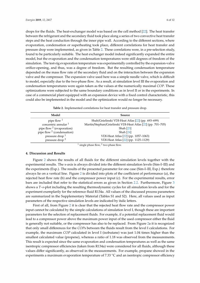
Table 2. Implemented correlations for heat transfer and pressure drop.

Model Source

pipe flow 1 Shah/Gnielinski VDI-Heat Atlas [22] (pp. 693–699)concentric annular 1 Martin/Stephan/Gnielinski VDI-Heat Atlas [22] (pp. 701–705)

pipe flow 2 (evaporation) Shah [23]pipe flow 2 (condensation) Shah [24]

pressure drop 1 VDI-Heat Atlas [22] (pp. 1057–1063)pressure drop 2 VDI-Heat Atlas [22] (pp. 1125–1129)

1 single phase flow, 2 two phase flow.

4. Discussion and Results

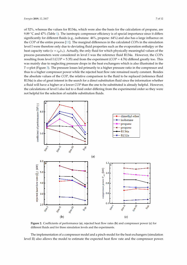
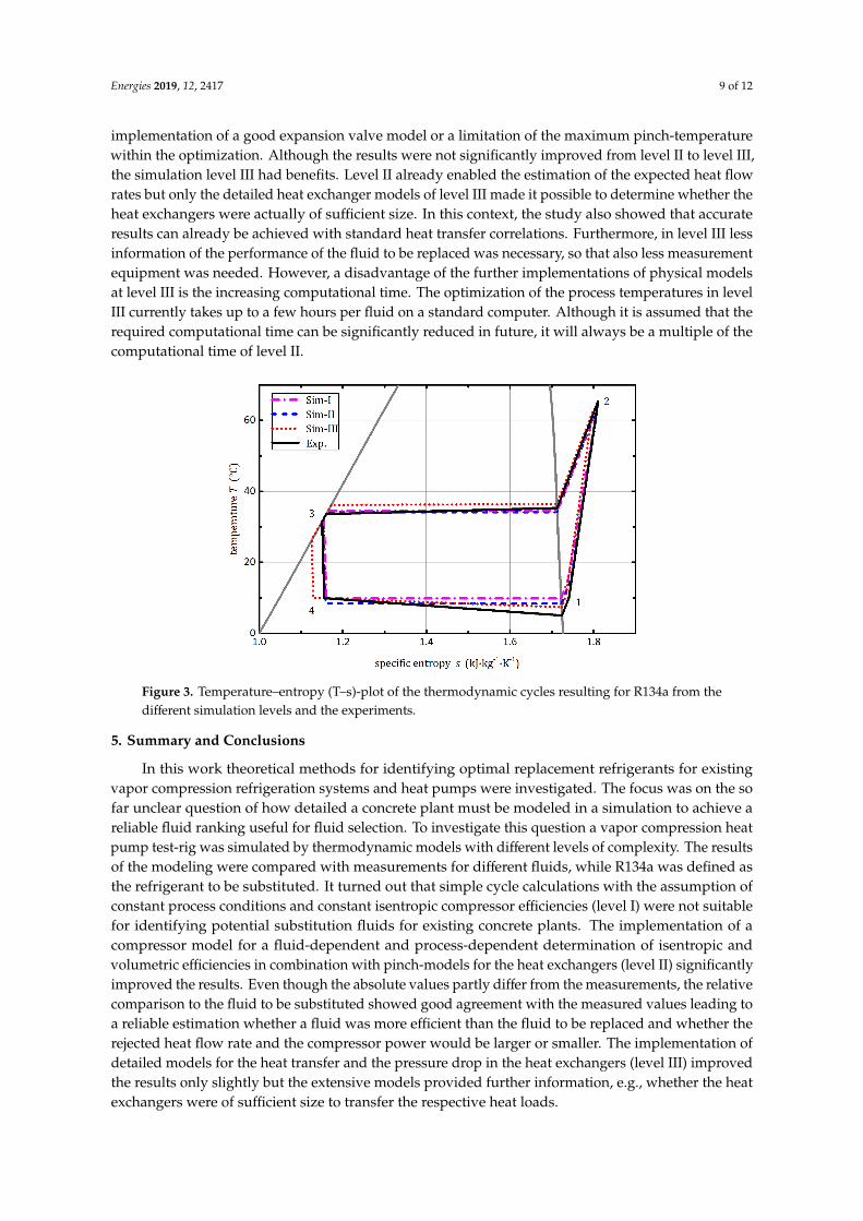
Figure 2 shows the results of all fluids for the different simulation levels together with theexperimental results. The x-axis is always divided into the different simulation levels (Sim-I–III) andthe experiments (Exp.). The results of the presented parameter for one case (Sim-I–III, Exp.) thereforealways lie on a vertical line. Figure 2 is divided into plots of the coefficient of performance (a), therejected heat flow rate (b) and the compressor power input (c). For the experimental results, errorbars are included that refer to the statistical errors as given in Section 2.2. Furthermore, Figure 3shows a T–s-plot including the resulting thermodynamic cycles for all simulation levels and for theexperiment exemplarily for the reference fluid R134a. All values of the discussed process parametersare summarized in the Supplementary Material (Tables S1 and S2). Here, all values used as inputparameters of the respective simulation levels are indicated by italic letters.

First of all, from Figure 2 it is clear that the rejected heat flow rate and the compressor powerinput cannot be calculated by the simple calculations of simulation level I, though these are importantparameters for the selection of replacement fluids. For example, if a potential replacement fluid wouldlead to a compressor power above the maximum power input of the used compressor either the fluidis generally not suitable, or the compressor has also to be replaced. From Figure 2a it is recognizedthat only small differences for the COPs between the fluids result from the level I calculations. Forexample, the maximum COP calculated in level I (isobutane) was just 1.04 times higher than thesmallest calculated value (propene), whereas a ratio of 1.18 was observed from the measurements.This result is expected since the same evaporation and condensation temperatures as well as the sameisentropic compressor efficiencies (taken from R134a) were considered for all fluids, although thesevalues differ significantly, as observed in the measurements. For example, propane showed in theexperiments a maximum evaporation temperature of 7.33 ◦C and an isentropic compressor efficiency

Energies 2019, 12, 2417 7 of 12

of 52%, whereas the values for R134a, which were also the basis for the calculation of propane, are9.89 ◦C and 47% (Table 1). The isentropic compressor efficiency is of special importance since it differssignificantly for different fluids (e.g., isobutane: 46%, propene: 64%) and also has a large influence onthe COP of the entire process [11]. The marginal differences in the calculated COPs in the simulationlevel I were therefore only due to deviating fluid properties such as the evaporation enthalpy or theheat capacity ratio (κ = cp/cv). Actually, the only fluid for which physically meaningful values of theprocess parameters were considered in level I was the reference fluid R134a. However, the COPsresulting from level I (COP = 5.35) and from the experiment (COP = 4.76) differed greatly too. Thiswas mainly due to neglecting pressure drops in the heat exchangers which is also illustrated in theT–s-plot (Figure 3). The pressure losses led primarily to a higher pressure ratio in the compressor andthus to a higher compressor power while the rejected heat flow rate remained nearly constant. Besidesthe absolute values of the COP, the relative comparison to the fluid to be replaced (reference fluidR134a) is also of great interest in the search for a direct substitution fluid since the information whethera fluid will have a higher or a lower COP than the one to be substituted is already helpful. However,the calculations of level I also led to a fluid order differing from the experimental order so they werenot helpful for the selection of suitable substitution fluids.

Energies 2019, 12, x FOR PEER REVIEW 7 of 12

although these values differ significantly, as observed in the measurements. For example, propane showed in the experiments a maximum evaporation temperature of 7.33 °C and an isentropic compressor efficiency of 52%, whereas the values for R134a, which were also the basis for the calculation of propane, are 9.89 °C and 47% (Table 1). The isentropic compressor efficiency is of special importance since it differs significantly for different fluids (e.g., isobutane: 46%, propene: 64%) and also has a large influence on the COP of the entire process [11]. The marginal differences in the calculated COPs in the simulation level I were therefore only due to deviating fluid properties such as the evaporation enthalpy or the heat capacity ratio (κ = cp/cv). Actually, the only fluid for which physically meaningful values of the process parameters were considered in level I was the reference fluid R134a. However, the COPs resulting from level I (COP = 5.35) and from the experiment (COP = 4.76) differed greatly too. This was mainly due to neglecting pressure drops in the heat exchangers which is also illustrated in the T–s-plot (Figure 3). The pressure losses led primarily to a higher pressure ratio in the compressor and thus to a higher compressor power while the rejected heat flow rate remained nearly constant. Besides the absolute values of the COP, the relative comparison to the fluid to be replaced (reference fluid R134a) is also of great interest in the search for a direct substitution fluid since the information whether a fluid will have a higher or a lower COP than the one to be substituted is already helpful. However, the calculations of level I also led to a fluid order differing from the experimental order so they were not helpful for the selection of suitable substitution fluids.

(a)

(b) (c)

Figure 2. Coefficients of performance (a), rejected heat flow rates (b) and compressor power (c) for different fluids and for three simulation levels and the experiments.

Figure 2. Coefficients of performance (a), rejected heat flow rates (b) and compressor power (c) fordifferent fluids and for three simulation levels and the experiments.

The implementation of a compressor model and a pinch-model for the heat exchangers (simulationlevel II) also allows the model to estimate the expected heat flow rate and the compressor power.

Energies 2019, 12, 2417 8 of 12

Regarding the COPs in Figure 1, the results are now significantly improved, although a comparisonwith the measured values shows that the calculated COPs were, averaged over all fluids, about 14% toolarge. The situation is similar for the rejected heat flow rates; the calculated values were all too large.On the other hand, the values of compressor power were predicted with only small deviations (≈ 3.5%).The deviations were again mainly due to the neglect of the pressure losses (Figure 3). Neglectingthe pressure loss in the evaporator led to a too high pressure at the compressor inlet and thus toa decreased specific volume and to a smaller pressure ratio. The smaller pressure ratio caused adecreased specific compressor work while the decreased specific volume at the compressor inlet led toincreased mass flow rates. Since the specific rejected heat remained nearly constant, the calculatedheat flow rates were largely too high. Coincidentally, there were two counteracting effects in thecompressor. The underestimated specific compressor work was counteracted by the overestimatedmass flow rates so that overall the calculated values of the compressor power differed only slightlyfrom the measurements. As a result, the calculations of level II led to overestimated COPs. Therelative comparison to the fluid to be substituted showed that the simulation level II already led toadequate results. Based on the calculated values, it is possible to estimate with good accuracy whethera fluid will have higher or lower values of COP, rejected heat flow rate and compressor power, all incomparison to the previously used fluid. There are also some deviations. For example, it was predictedthat propane has a smaller COP compared to isobutane and R152a, contradicting the experiments. Inpractice, a significant advantage of propane was observed. Nevertheless, level II is a helpful tool for apre-selection step of suitable substitution fluids. If the resulting process of the fluid to be substitutedis known from the considered plant it can reliably be estimated whether a fluid will at least reachthe same rejected heat flow rate, whether it is compatible with the compressor installed, in termsof maximum power, and whether it will have a higher or a lower COP. The comparison with theresults of level I showed that a good model for the calculation of the fluid dependent compressorefficiency is indispensable while already simple and unspecific models for the heat exchangers lead toreasonable results. An additional advantage of the simulation level II was the low computation time.The calculation of one fluid running on a standard computer (CPU: Intel Core i7-4790, RAM: 24 GB)only took a few minutes so that even large fluid databases could be searched for suitable fluids in arelatively short time.

In addition to the compressor model, the simulation level III also included detailed modelsfor the calculation of heat transfer and pressure drop in the heat exchangers. This led in part toimproved results with respect to level II and a better agreement with the experiments, as obviousfrom Figure 2. Compared to the results of level II, the COPs were calculated to be significantlysmaller but they were still too high with respect to the measurements. The calculated order of fluidswith respect to their COPs was not significantly improved and the wrong assessment regardingpropane compared to isobutane and R134a remained. From the calculated rejected heat flow rates andcompressor power it becomes clear that the overestimated COPs resulted primarily from overestimatedheat flow rates since the calculated values of the compressor power fitted well to the measurements.In contrast to level II, the deviations here were not due to neglecting pressure drops. Rather, theoptimization of the condensation temperatures was prone to error. In real cycles, the condensationtemperature results from the interaction of all components. Due to a missing model for the expansionvalve, however, this could not be simulated here. Alternatively, the condensation temperature wasnumerically optimized with respect to maximum COP as described previously. However, it can beobserved from the data, and from the T–s-plot (Figure 3), that the numerical optimum was alwayslocated at unrealistically high condensation temperatures. The slightly overestimated condensationtemperatures led to increased temperature differences between the refrigerant and the secondary fluidin the condenser (the temperature change of the secondary fluid was constant) and thus to higher heatflow rates. This also led to an increased sub-cooling at the condenser outlet (Figure 3). Overestimatedheat flow rates at unchanged compressor power resulted in overestimated COPs. Because this effectwas of numerical origin it could not be observed in the experiments. A solution would be either the

Energies 2019, 12, 2417 9 of 12

implementation of a good expansion valve model or a limitation of the maximum pinch-temperaturewithin the optimization. Although the results were not significantly improved from level II to level III,the simulation level III had benefits. Level II already enabled the estimation of the expected heat flowrates but only the detailed heat exchanger models of level III made it possible to determine whether theheat exchangers were actually of sufficient size. In this context, the study also showed that accurateresults can already be achieved with standard heat transfer correlations. Furthermore, in level III lessinformation of the performance of the fluid to be replaced was necessary, so that also less measurementequipment was needed. However, a disadvantage of the further implementations of physical modelsat level III is the increasing computational time. The optimization of the process temperatures in levelIII currently takes up to a few hours per fluid on a standard computer. Although it is assumed that therequired computational time can be significantly reduced in future, it will always be a multiple of thecomputational time of level II.

Energies 2019, 12, x FOR PEER REVIEW 9 of 12

experiments. A solution would be either the implementation of a good expansion valve model or a limitation of the maximum pinch-temperature within the optimization. Although the results were not significantly improved from level II to level III, the simulation level III had benefits. Level II already enabled the estimation of the expected heat flow rates but only the detailed heat exchanger models of level III made it possible to determine whether the heat exchangers were actually of sufficient size. In this context, the study also showed that accurate results can already be achieved with standard heat transfer correlations. Furthermore, in level III less information of the performance of the fluid to be replaced was necessary, so that also less measurement equipment was needed. However, a disadvantage of the further implementations of physical models at level III is the increasing computational time. The optimization of the process temperatures in level III currently takes up to a few hours per fluid on a standard computer. Although it is assumed that the required computational time can be significantly reduced in future, it will always be a multiple of the computational time of level II.

Figure 3. Temperature–entropy (T–s)-plot of the thermodynamic cycles resulting for R134a from the different simulation levels and the experiments.

5. Summary and Conclusions

In this work theoretical methods for identifying optimal replacement refrigerants for existing vapor compression refrigeration systems and heat pumps were investigated. The focus was on the so far unclear question of how detailed a concrete plant must be modeled in a simulation to achieve a reliable fluid ranking useful for fluid selection. To investigate this question a vapor compression heat pump test-rig was simulated by thermodynamic models with different levels of complexity. The results of the modeling were compared with measurements for different fluids, while R134a was defined as the refrigerant to be substituted. It turned out that simple cycle calculations with the assumption of constant process conditions and constant isentropic compressor efficiencies (level I) were not suitable for identifying potential substitution fluids for existing concrete plants. The implementation of a compressor model for a fluid-dependent and process-dependent determination of isentropic and volumetric efficiencies in combination with pinch-models for the heat exchangers (level II) significantly improved the results. Even though the absolute values partly differ from the measurements, the relative comparison to the fluid to be substituted showed good agreement with the measured values leading to a reliable estimation whether a fluid was more efficient than the fluid to be replaced and whether the rejected heat flow rate and the compressor power would be larger or smaller. The implementation of detailed models for the heat transfer and the pressure drop in the heat exchangers (level III) improved the results only slightly but the extensive models

Figure 3. Temperature–entropy (T–s)-plot of the thermodynamic cycles resulting for R134a from thedifferent simulation levels and the experiments.

5. Summary and Conclusions

In this work theoretical methods for identifying optimal replacement refrigerants for existingvapor compression refrigeration systems and heat pumps were investigated. The focus was on the sofar unclear question of how detailed a concrete plant must be modeled in a simulation to achieve areliable fluid ranking useful for fluid selection. To investigate this question a vapor compression heatpump test-rig was simulated by thermodynamic models with different levels of complexity. The resultsof the modeling were compared with measurements for different fluids, while R134a was defined asthe refrigerant to be substituted. It turned out that simple cycle calculations with the assumption ofconstant process conditions and constant isentropic compressor efficiencies (level I) were not suitablefor identifying potential substitution fluids for existing concrete plants. The implementation of acompressor model for a fluid-dependent and process-dependent determination of isentropic andvolumetric efficiencies in combination with pinch-models for the heat exchangers (level II) significantlyimproved the results. Even though the absolute values partly differ from the measurements, the relativecomparison to the fluid to be substituted showed good agreement with the measured values leading toa reliable estimation whether a fluid was more efficient than the fluid to be replaced and whether therejected heat flow rate and the compressor power would be larger or smaller. The implementation ofdetailed models for the heat transfer and the pressure drop in the heat exchangers (level III) improvedthe results only slightly but the extensive models provided further information, e.g., whether the heatexchangers were of sufficient size to transfer the respective heat loads.

Energies 2019, 12, 2417 10 of 12

In summary, the study has shown that a good model for calculating compressor efficiencies isthe minimum requirement for an effective search for replacement fluids for a specific plant. Thecompressor model used here can also be applied to other reciprocating compressors. For the modelfitting only the four geometric parameters must be known as well as the isentropic and volumetricefficiencies for one operating point with one fluid. If different compressor types (screw, scroll etc.) areinstalled, the compressor model must be replaced accordingly. For the heat exchangers, it was shownthat simple pinch-models are, at least for a preselection step, already a good approach which can easilybe applied also to other types of heat exchangers (plate heat exchangers, crossflow etc.). However, thisdoes not apply to the extensive model used here (level III) as it was developed only for double-pipeheat exchangers. Nevertheless, similar models can also be designed for other types of heat exchangers.In the future, software that includes models for different types of compressors and heat exchangerswhich can be individually combined with respect to the specific plant would be very helpful.

Due to the high computational effort of level III compared to level II, the high complexity modelis not recommended to scan large refrigerant databases. Rather, it is recommended to carry outa preliminary study at level II and then to consider some of the identified fluids with a detailedmodel at level III. Although the simulations do not replace final experimental tests, they should bevery helpful to select a reduced number of potential substitution fluids and reduce the number ofrequired experiments.

Supplementary Materials: The following are available online at http://www.mdpi.com/1996-1073/12/12/2417/s1,Table S1: Data of dimethyl ether, isobutane and propane. Table S2: Data of propene, R134a and R152a. Thesetables provide the values of all discussed process parameters for all simulation levels and for the experiments.Italic letters indicate input values of the simulations and regular letters specify results.

Author Contributions: D.R. conceived the present idea and developed and carried out the simulations. V.V.planned and carried out the experiments. B.A. was the project administrator, supervised the project and was incharge of the overall direction. Result processing and interpretation was a joint process.

Funding: This research received no external funding.

Conflicts of Interest: The authors declare no conflicts of interest.

Nomenclature

I, II, III simulation levelsccl relative clearance volume (compressor model)cp isobaric heat capacity, J·kg−1

·K−1

cv isochoric heat capacity, J·kg−1·K−1

→g vector of constraint functionsh specific enthalpy, J·kg−1.

m refrigerant mass flow rate, kg·s−1

Pcom electrical compressor power, Wp pressure, Papfr friction pressure (compressor model), Pa.

QH rejected heat flow rate (condenser), WqH specific rejected heat (condenser), J·kg−1

s specific entropy, J·kg−1·K−1

T temperature, K or ◦Cwcom specific compressor work, J·kg−1

Greek symbols∆i difference of iηs

com sentropic compressor efficiencyκ heat capacity ratio

Energies 2019, 12, 2417 11 of 12

Subscripts and superscripts1, 2, 3, 4 cycle statesc condensercom compressorev evaporatori inletmax maximummin minimumo outletw secondary heat transfer fluid water

References

1. United Nations Environment Progamme UNEP. Montreal Protocol on Substances that Deplete the OzoneLayer. 1987. Available online: www.unep.org (accessed on 21 June 2019).

2. European Union. Verordnung über Fluorierte Treibhausgase; EU: Brussels, Belgium, 2014; p. 517.3. Intergovernmental Panel on Climate Change (IPCC). Working Group I Contribution to the IPCC Fifth

Assessment Report: Climate Change 2013: The Physical Science Basis. Available online: http://www.climatechange2013.org/images/uploads/WGIAR5_WGI-12Doc2b_FinalDraft_Chapter08.pdf (accessed on21 June 2019).

4. Honeywell Deutschland. Solstice Kältemittel: Roadmap. Available online: https://www.honeywell-refrigerants.com/europe/wp-content/uploads/2017/05/FPR-004-2017-10-DE_Refrigerants_Roadmap_LR.pdf (accessed on 21 June 2019).

5. Li, Z.; Liang, K.; Jiang, H. Experimental study of R1234yf as a drop-in replacement for R134a in an oil-freerefrigeration system. Appl. Therm. Eng. 2019, 153, 646–654. [CrossRef]

6. Sánchez, D.; Cabello, R.; Llopis, R.; Arauzo, I.; Catalán-Gil, J.; Torrella, E. Energy performance evaluation ofR1234yf, R1234ze(E), R600a, R290 and R152a as low-GWP R134a alternatives. Int. J. Refrig. 2017, 74, 269–282.[CrossRef]

7. Brown, J.S. Predicting performance of refrigerants using the Peng–Robinson Equation of State. Int. J. Refrig.2007, 30, 1319–1328. [CrossRef]

8. Dalkilic, A.S.; Wongwises, S. A performance comparison of vapour-compression refrigeration system usingvarious alternative refrigerants. Int. Commun. Heat Mass Transf. 2010, 37, 1340–1349. [CrossRef]

9. Saleh, B.; Wendland, M. Screening of pure fluids as alternative refrigerants. Int. J. Refrig. 2006, 29, 260–269.[CrossRef]

10. Roskosch, D.; Atakan, B. Reverse engineering of fluid selection for thermodynamic cycles with cubicequations of state, using a compression heat pump as example. Energy 2015, 81, 202–212. [CrossRef]

11. Venzik, V.; Roskosch, D.; Atakan, B. Propene/isobutane mixtures in heat pumps: An experimentalinvestigation. Int. J. Refrig. 2017, 76, 84–96. [CrossRef]

12. Fang, Y.; Croquer, S.; Poncet, S.; Aidoun, Z.; Bartosiewicz, Y. Drop-in replacement in a R134 ejectorrefrigeration cycle by HFO refrigerants. Int. J. Refrig. 2017, 77, 87–98. [CrossRef]

13. Cabello, R.; Sánchez, D.; Llopis, R.; Arauzo, I.; Torrella, E. Experimental comparison between R152a andR134a working in a refrigeration facility equipped with a hermetic compressor. Int. J. Refrig. 2015, 60, 92–105.[CrossRef]

14. Chang, Y.; Kim, M.; Ro, S. Performance and heat transfer characteristics of hydrocarbon refrigerants in a heatpump system. Int. J. Refrig. 2000, 23, 232–242. [CrossRef]

15. Mendoza-Miranda, J.M.; Mota-Babiloni, A.; Ramírez-Minguela, J.J.; Muñoz-Carpio, V.D.; Carrera-Rodríguez, M.;Navarro-Esbrí, J.; Salazar-Hernández, C. Comparative evaluation of R1234yf, R1234ze(E) and R450A asalternatives to R134a in a variable speed reciprocating compressor. Energy 2016, 114, 753–766. [CrossRef]

16. Miyara, A. Condensation of hydrocarbons–A review. Int. J. Refrig. 2008, 31, 621–632. [CrossRef]17. National Instruments. LabVIEW Professional Development System; National Instruments: Austin, TX, USA, 2013.18. Lemmon, E.W.; Huber, M.L.; McLinden, M.O. NIST Standard Reference Database 23; National Institute of

Standards and Technology: Gaithersburg, MD, USA, 2013.19. Python.org. Available online: https://www.python.org/ (accessed on 21 June 2019).

Energies 2019, 12, 2417 12 of 12

20. OpenOpt. Available online: http://openopt.blogspot.de/ (accessed on 21 June 2019).21. Roskosch, D.; Venzik, V.; Atakan, B. Thermodynamic model for reciprocating compressors with the focus on

fluid dependent efficiencies. Int. J. Refrig. 2017, 84, 104–116. [CrossRef]22. Ingenieure, V.D. VDI Heat Atlas, 2nd ed.; Springer: Berlin, Germany, 2010; ISBN 978-3-540-77877-6.23. Shah, M.M. A New Correlation for Heat Transfer During Boiling Flow Through Pipes. Ashrae Trans. 1976,

66–86.24. Shah, M.M. A general correlation for heat transfer during film condensation inside pipes. Int. J. Heat

Mass Transf. 1979, 22, 547–556. [CrossRef]

© 2019 by the authors. Licensee MDPI, Basel, Switzerland. This article is an open accessarticle distributed under the terms and conditions of the Creative Commons Attribution(CC BY) license (http://creativecommons.org/licenses/by/4.0/).

Fluid Retrofit for Existing Vapor Compression Refrigeration Systems and

Heat Pumps

Roskosch, Dennis; Venzik, Valerius; Atakan, Burak

This text is provided by DuEPublico, the central repository of the University Duisburg-Essen.

This version of the e-publication may differ from a potential published print or online version.

DOI: https://doi.org/10.3390/en12122417

URN: urn:nbn:de:hbz:464-20190814-115233-9

Link: https://duepublico.uni-duisburg-essen.de:443/servlets/DocumentServlet?id=49175

License:

This work may be used under a Creative Commons Attribution 4.0 International license.

Source: Energies 2019, 12, 2417; Published: 24 June 2019