REGIONAL ANALYSIS OF EXTREME PRECIPITATION

EVENTS IN THE CZECH REPUBLIC

Jan Kyselý1, Jan Picek2 and Radan Huth1 1 Institute of Atmospheric Physics AV CR, Prague, Czech Republic (e-mail: honza@ufa.cas.cz), 2 Technical University, Liberec, Czech Republic (e-mail: jan.picek@vslib.cz)

Acknowledgement: The study is supported by the Grant Agency of the Academy of Sciences of the Czech Republic under project B3042303. Thanks are due to J.Hošek for assistance in drawing the figures.

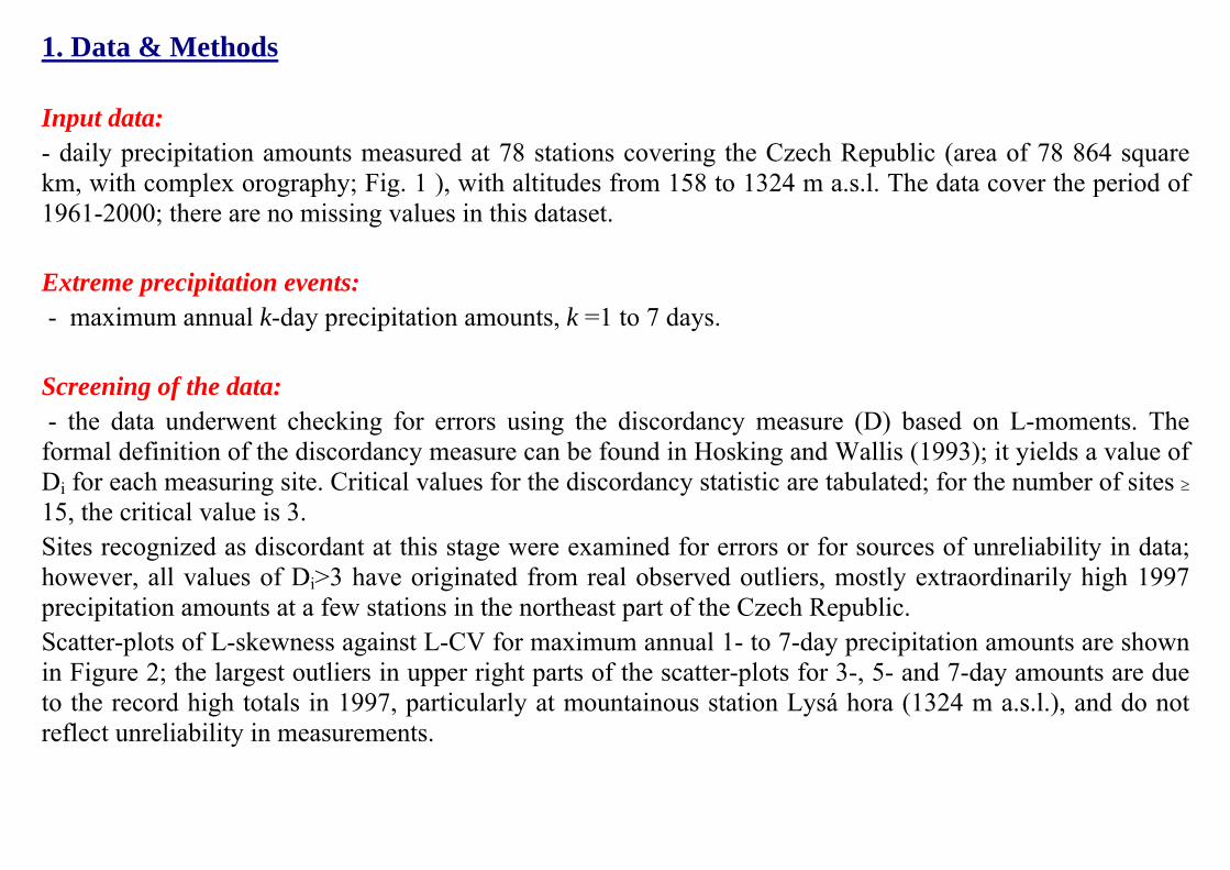
1. Data & Methods

Input data: - daily precipitation amounts measured at 78 stations covering the Czech Republic (area of 78 864 square km, with complex orography; Fig. 1 ), with altitudes from 158 to 1324 m a.s.l. The data cover the period of 1961-2000; there are no missing values in this dataset. Extreme precipitation events: - maximum annual k-day precipitation amounts, k =1 to 7 days. Screening of the data: - the data underwent checking for errors using the discordancy measure (D) based on L-moments. The formal definition of the discordancy measure can be found in Hosking and Wallis (1993); it yields a value of Di for each measuring site. Critical values for the discordancy statistic are tabulated; for the number of sites ≥ 15, the critical value is 3. Sites recognized as discordant at this stage were examined for errors or for sources of unreliability in data; however, all values of Di>3 have originated from real observed outliers, mostly extraordinarily high 1997 precipitation amounts at a few stations in the northeast part of the Czech Republic. Scatter-plots of L-skewness against L-CV for maximum annual 1- to 7-day precipitation amounts are shown in Figure 2; the largest outliers in upper right parts of the scatter-plots for 3-, 5- and 7-day amounts are due to the record high totals in 1997, particularly at mountainous station Lysá hora (1324 m a.s.l.), and do not reflect unreliability in measurements.

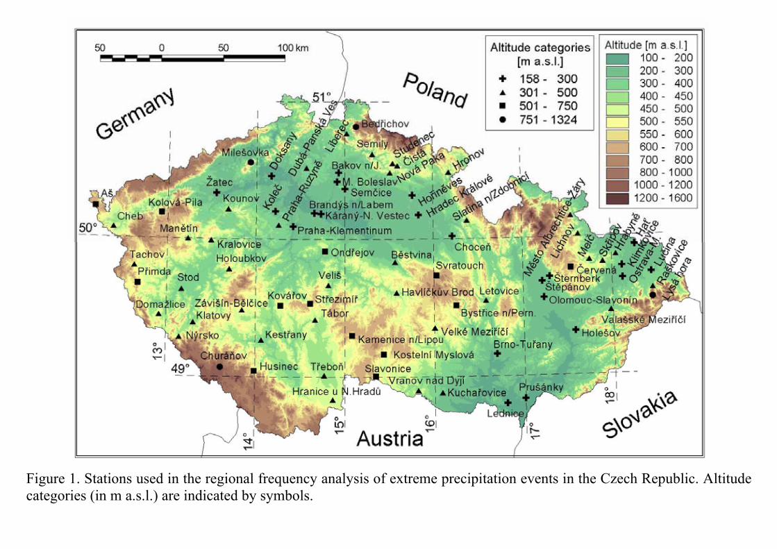
Figure 1. Stations used in the regional frequency analysis of extreme precipitation events in the Czech Republic. Altitude categories (in m a.s.l.) are indicated by symbols.

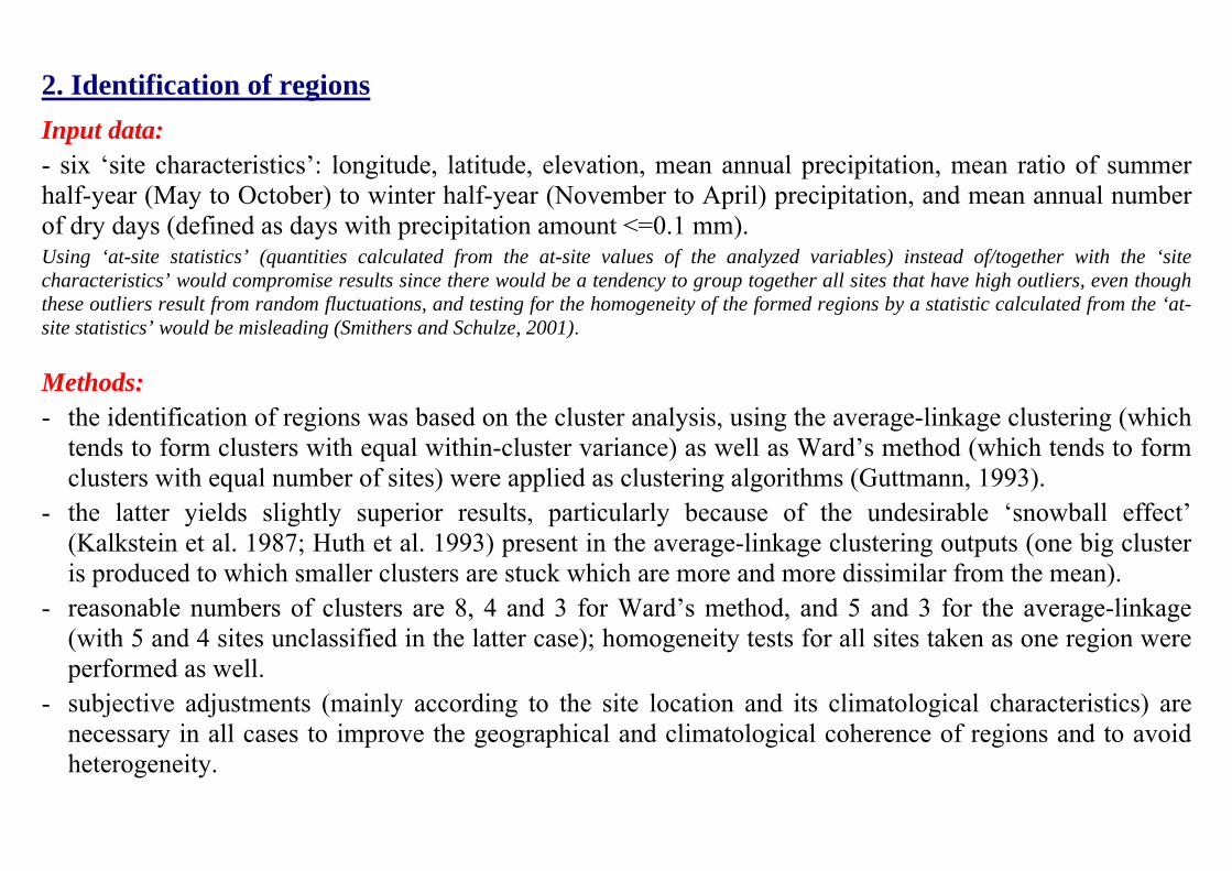
2. Identification of regions Input data: - six ‘site characteristics’: longitude, latitude, elevation, mean annual precipitation, mean ratio of summer half-year (May to October) to winter half-year (November to April) precipitation, and mean annual number of dry days (defined as days with precipitation amount <=0.1 mm). Using ‘at-site statistics’ (quantities calculated from the at-site values of the analyzed variables) instead of/together with the ‘site characteristics’ would compromise results since there would be a tendency to group together all sites that have high outliers, even though these outliers result from random fluctuations, and testing for the homogeneity of the formed regions by a statistic calculated from the ‘at-site statistics’ would be misleading (Smithers and Schulze, 2001).

Methods: - the identification of regions was based on the cluster analysis, using the average-linkage clustering (which

tends to form clusters with equal within-cluster variance) as well as Ward’s method (which tends to form clusters with equal number of sites) were applied as clustering algorithms (Guttmann, 1993).

- the latter yields slightly superior results, particularly because of the undesirable ‘snowball effect’ (Kalkstein et al. 1987; Huth et al. 1993) present in the average-linkage clustering outputs (one big cluster is produced to which smaller clusters are stuck which are more and more dissimilar from the mean).

- reasonable numbers of clusters are 8, 4 and 3 for Ward’s method, and 5 and 3 for the average-linkage (with 5 and 4 sites unclassified in the latter case); homogeneity tests for all sites taken as one region were performed as well.

- subjective adjustments (mainly according to the site location and its climatological characteristics) are necessary in all cases to improve the geographical and climatological coherence of regions and to avoid heterogeneity.

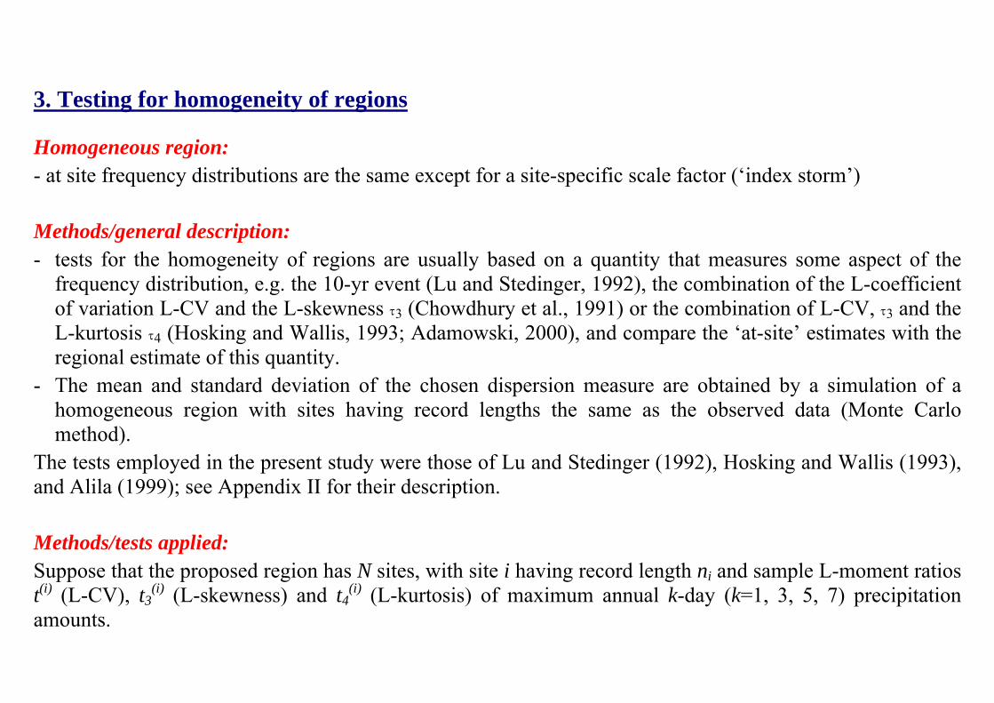
3. Testing for homogeneity of regions

Homogeneous region: - at site frequency distributions are the same except for a site-specific scale factor (‘index storm’) Methods/general description: - tests for the homogeneity of regions are usually based on a quantity that measures some aspect of the

frequency distribution, e.g. the 10-yr event (Lu and Stedinger, 1992), the combination of the L-coefficient of variation L-CV and the L-skewness τ3 (Chowdhury et al., 1991) or the combination of L-CV, τ3 and the L-kurtosis τ4 (Hosking and Wallis, 1993; Adamowski, 2000), and compare the ‘at-site’ estimates with the regional estimate of this quantity.

- The mean and standard deviation of the chosen dispersion measure are obtained by a simulation of a homogeneous region with sites having record lengths the same as the observed data (Monte Carlo method).

The tests employed in the present study were those of Lu and Stedinger (1992), Hosking and Wallis (1993), and Alila (1999); see Appendix II for their description. Methods/tests applied: Suppose that the proposed region has N sites, with site i having record length ni and sample L-moment ratios t(i) (L-CV), t3

(i) (L-skewness) and t4(i) (L-kurtosis) of maximum annual k-day (k=1, 3, 5, 7) precipitation

amounts.

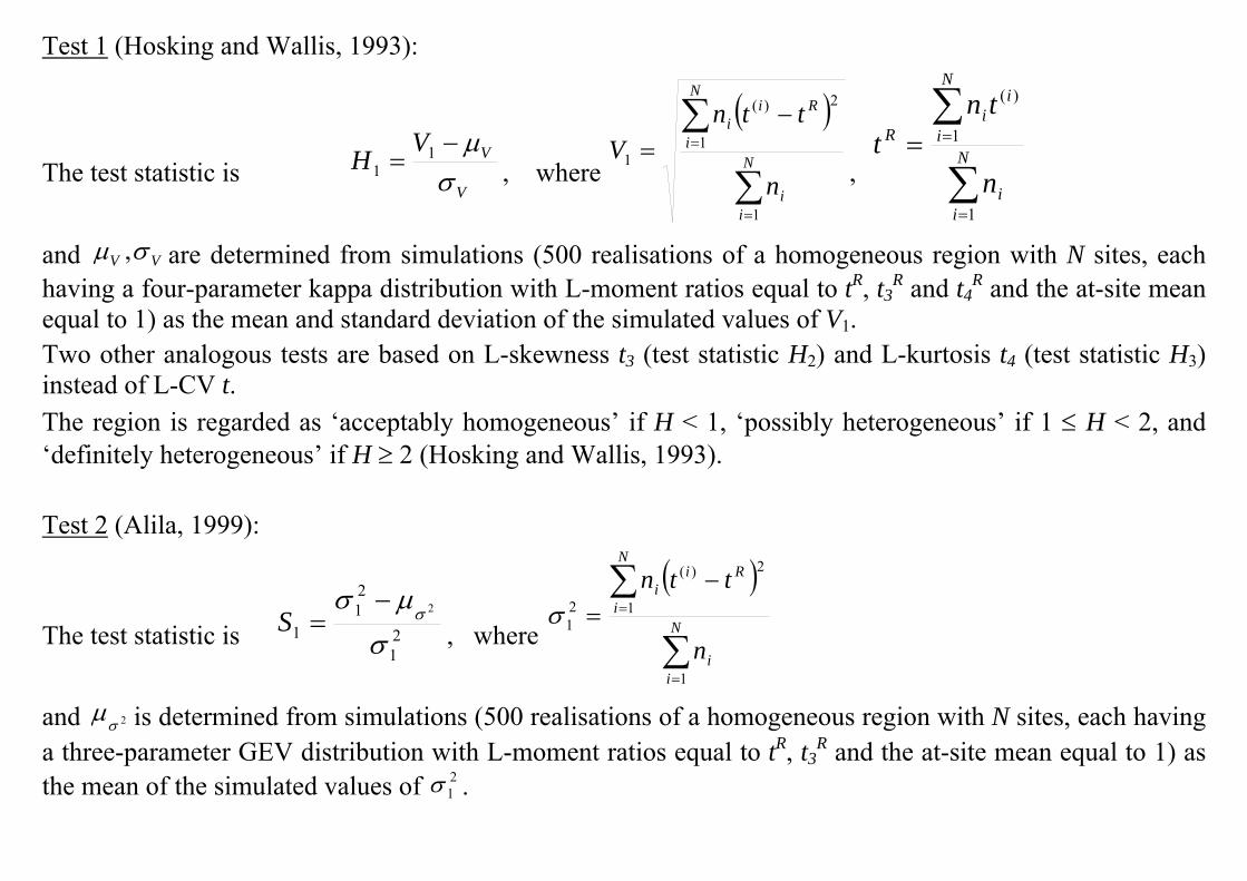
Test 1 (Hosking and Wallis, 1993):

The test statistic is V

VVH

σµ−

= 11 , where

( )

∑

∑

=

=

−= N

ii

N

i

Rii

n

ttnV

1

1

2)(

1 , ∑

∑

=

== N

ii

N

i

ii

R

n

tnt

1

1

)(

and VV σµ , are determined from simulations (500 realisations of a homogeneous region with N sites, each having a four-parameter kappa distribution with L-moment ratios equal to tR, t3

R and t4R and the at-site mean

equal to 1) as the mean and standard deviation of the simulated values of V1. Two other analogous tests are based on L-skewness t3 (test statistic H2) and L-kurtosis t4 (test statistic H3) instead of L-CV t. The region is regarded as ‘acceptably homogeneous’ if H < 1, ‘possibly heterogeneous’ if 1 ≤ H < 2, and ‘definitely heterogeneous’ if H ≥ 2 (Hosking and Wallis, 1993). Test 2 (Alila, 1999):

The test statistic is 21

21

12

σµσσ

−=S , where

( )

∑

∑

=

=

−= N

ii

N

i

Rii

n

ttn

1

1

2)(

21σ

and 2σµ is determined from simulations (500 realisations of a homogeneous region with N sites, each having

a three-parameter GEV distribution with L-moment ratios equal to tR, t3R and the at-site mean equal to 1) as

the mean of the simulated values of 21σ .

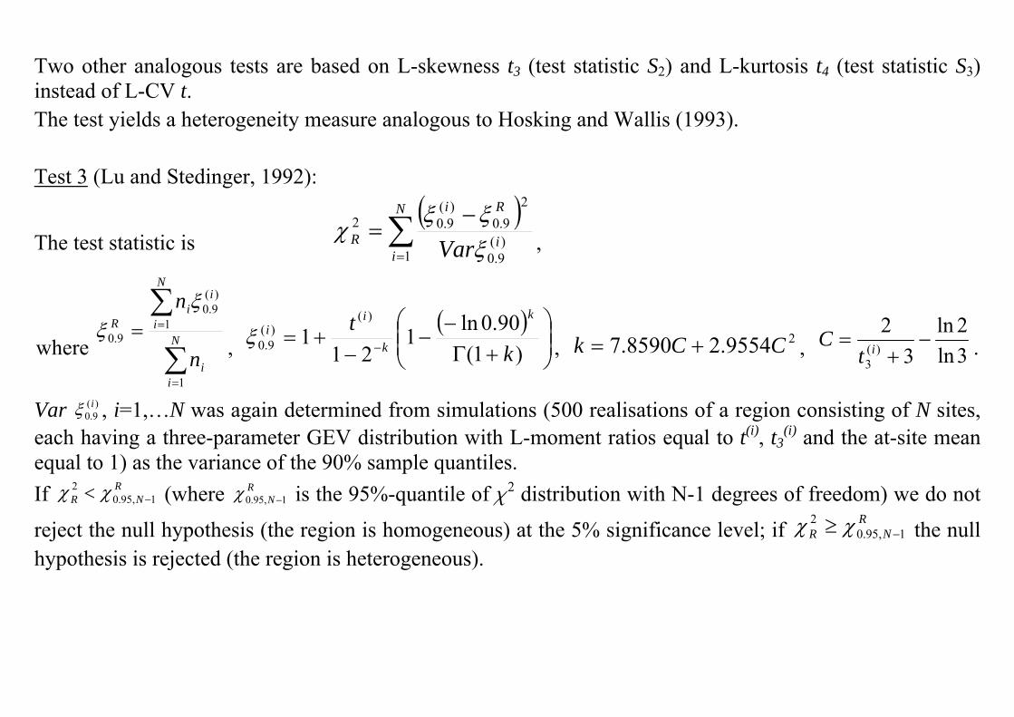
Two other analogous tests are based on L-skewness t3 (test statistic S2) and L-kurtosis t4 (test statistic S3) instead of L-CV t. The test yields a heterogeneity measure analogous to Hosking and Wallis (1993). Test 3 (Lu and Stedinger, 1992):

The test statistic is ( )∑

=

−=

N

ii

Ri

R Var1)(9.0

29.0

)(9.02

ξξξ

χ ,

where ∑

∑

=

== N

ii

N

i

ii

R

n

n

1

1

)(9.0

9.0

ξξ

, ( )

⎟⎟⎠

⎞⎜⎜⎝

⎛+Γ

−−

−+= − )1(

90.0ln121

1)(

)(9.0 k

t k

k

iiξ , 29554.28590.7 CCk += , 3ln

2ln3

2)(

3

−+

= itC .

Var )(9.0iξ , i=1,…N was again determined from simulations (500 realisations of a region consisting of N sites,

each having a three-parameter GEV distribution with L-moment ratios equal to t(i), t3(i) and the at-site mean

equal to 1) as the variance of the 90% sample quantiles. If R

NR 1,95.02

−< χχ (where RN 1,95.0 −χ is the 95%-quantile of c2 distribution with N-1 degrees of freedom) we do not

reject the null hypothesis (the region is homogeneous) at the 5% significance level; if RNR 1,95.0

2−≥ χχ the null

hypothesis is rejected (the region is heterogeneous).

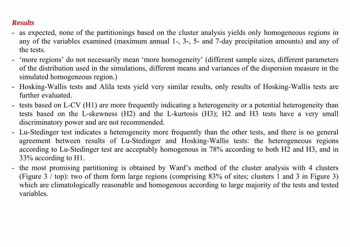
Results - as expected, none of the partitionings based on the cluster analysis yields only homogeneous regions in

any of the variables examined (maximum annual 1-, 3-, 5- and 7-day precipitation amounts) and any of the tests.

- ‘more regions’ do not necessarily mean ‘more homogeneity’ (different sample sizes, different parameters of the distribution used in the simulations, different means and variances of the dispersion measure in the simulated homogeneous region.)

- Hosking-Wallis tests and Alila tests yield very similar results, only results of Hosking-Wallis tests are further evaluated.

- tests based on L-CV (H1) are more frequently indicating a heterogeneity or a potential heterogeneity than tests based on the L-skewness (H2) and the L-kurtosis (H3); H2 and H3 tests have a very small discriminatory power and are not recommended.

- Lu-Stedinger test indicates a heterogeneity more frequently than the other tests, and there is no general agreement between results of Lu-Stedinger and Hosking-Wallis tests: the heterogeneous regions according to Lu-Stedinger test are acceptably homogenous in 78% according to both H2 and H3, and in 33% according to H1.

- the most promising partitioning is obtained by Ward’s method of the cluster analysis with 4 clusters (Figure 3 / top): two of them form large regions (comprising 83% of sites; clusters 1 and 3 in Figure 3) which are climatologically reasonable and homogenous according to large majority of the tests and tested variables.

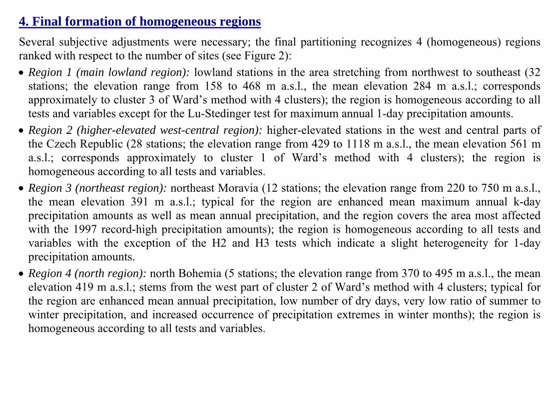
4. Final formation of homogeneous regions Several subjective adjustments were necessary; the final partitioning recognizes 4 (homogeneous) regions ranked with respect to the number of sites (see Figure 2): • Region 1 (main lowland region): lowland stations in the area stretching from northwest to southeast (32

stations; the elevation range from 158 to 468 m a.s.l., the mean elevation 284 m a.s.l.; corresponds approximately to cluster 3 of Ward’s method with 4 clusters); the region is homogeneous according to all tests and variables except for the Lu-Stedinger test for maximum annual 1-day precipitation amounts.

• Region 2 (higher-elevated west-central region): higher-elevated stations in the west and central parts of the Czech Republic (28 stations; the elevation range from 429 to 1118 m a.s.l., the mean elevation 561 m a.s.l.; corresponds approximately to cluster 1 of Ward’s method with 4 clusters); the region is homogeneous according to all tests and variables.

• Region 3 (northeast region): northeast Moravia (12 stations; the elevation range from 220 to 750 m a.s.l., the mean elevation 391 m a.s.l.; typical for the region are enhanced mean maximum annual k-day precipitation amounts as well as mean annual precipitation, and the region covers the area most affected with the 1997 record-high precipitation amounts); the region is homogeneous according to all tests and variables with the exception of the H2 and H3 tests which indicate a slight heterogeneity for 1-day precipitation amounts.

• Region 4 (north region): north Bohemia (5 stations; the elevation range from 370 to 495 m a.s.l., the mean elevation 419 m a.s.l.; stems from the west part of cluster 2 of Ward’s method with 4 clusters; typical for the region are enhanced mean annual precipitation, low number of dry days, very low ratio of summer to winter precipitation, and increased occurrence of precipitation extremes in winter months); the region is homogeneous according to all tests and variables.

Mountainous station Lysá hora (1324 m a.s.l.) is unclassified; its inclusion in region 3 leads to a considerable distortion of its homogeneity. Whether this is only due to sampling variability, or reflects real different features of the distribution of extreme high precipitation amounts cannot be concluded without additional precipitation data from the complex terrain of the northeast region. A major advantage of the 4 regions formed is that – apart from their homogeneity in statistical characteristics of extreme one-day and multi-day precipitation amounts – they are reasonable also from the point of view of precipitation climatology. The two main regions distinguish between lowland (region 1) and higher-elevated (region 2) locations in most of the area of the Czech Republic; taken together they do not form a homogeneous region. Climatological differences between these two regions consist mainly in larger mean annual precipitation amounts, smaller number of dry days, and a lower ratio of summer to winter precipitation at the higher-elevated sites, whereas mean annual k-day precipitation maxima are comparable in both regions. The two smaller regions possess distinctly different precipitation regimes, with enhanced mean annual precipitation and mean maximum annual k-day precipitation amounts (region 3), most likely due to orographic effects combined with a higher influence of slowly moving Mediterranean cyclones in the northeast part of the Czech Republic (Hanslian et al., 2000); and with enhanced mean annual precipitation, low number of dry days and increased precipitation (including extreme events) in winter at the expense of summer (region 4), due to a larger influence of cloud belts and atmospheric fronts associated with Atlantic cyclones in the prevailing southwestern to northwestern flow over the northernmost part of the Czech Republic which is close to the climatological location of the storm track over Europe in winter. Note that two northernmost stations Bedřichov and Liberec might rank among region 4 according to their locations as well as distinct characteristics of the precipitation regime, mainly a large percentage of precipitation, including extreme high amounts, falling in winter months. However, their incorporation into region 4 distorts the regional homogeneity, and their statistical characteristics of extreme precipitation events seem to be in consent with the patterns of regions 1 (Liberec) and 2 (Bedřichov).

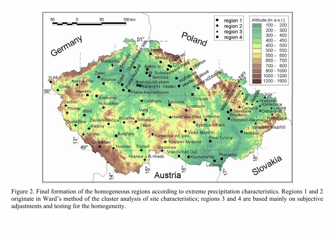
Figure 2. Final formation of the homogeneous regions according to extreme precipitation characteristics. Regions 1 and 2 originate in Ward’s method of the cluster analysis of site characteristics; regions 3 and 4 are based mainly on subjective adjustments and testing for the homogeneity.

5. Conclusions and prospective applications • The disastrous consequences of extreme high precipitation events, resulting in floods, may become

more pronounced in a future climate since an increase in their frequency and severity is expected and/or observed in large parts of Europe (IPCC, 2001). This research was motivated by the recent occurrence of severe summer floods (in 1997 and particularly 2002) in central Europe. It makes use of the development in environmental sciences, the L-moment based method of the regional frequency analysis, which has not been applied in studies dealing with return periods of hydrological extremes in the Czech Republic.

• The area of the Czech Republic has been divided into 4 homogeneous regions, based on the cluster analysis of site characteristics and tests for the homogeneity of the regions.

• The next step of the regional frequency analysis is the selection of the appropriate distribution of extreme precipitation events. GEV appears as the most appropriate distribution.

• The regions will enter next steps of the regional frequency analysis which concern the estimation of parameters and quantiles of the fitted distribution together with their uncertainty, with an emphasis on return periods of the 1997 and 2002 extreme precipitation events which caused massive floods in central Europe.

• Benefits of the regional frequency analysis of precipitation extremes compared to the at-site analysis will be evaluated.

Appendix: Definition of L-moments

Derivation of L-moments is based on order statistics which are obtained simply by sorting the sample {X1, X2, ..., Xn} of n independent realizations of variable X in ascending order {X1:n, X2:n, ..., Xn:n}; the subscript k:n denotes the k-th smallest number in the sample of length n. L-moments λk are defined as expectations of linear combinations of these order statistics, )( 1:11 XE=λ , )(

21

2:12:22 XXE −=λ ,

)2(31

3:13:23:33 XXXE +−=λ , and generally for the k-th L-moment

),(1

)1(1:

1

0kjk

k

j

jk XE

jk

k −

−

=⎟⎟⎠

⎞⎜⎜⎝

⎛ −−= ∑λ

where E denotes expectation operator (Hosking, 1990; von Storch and Zwiers, 1999). The first L-moment is the expected smallest value in a sample of one, i.e. the conventional first moment. The second L-moment is the expected absolute difference between any two realizations, multiplied by 1/2 (i.e., analogue to the conventional second moment). The third and fourth L-moments are shape parameters. L-moment

ratios (sometimes termed standardized L-moments) are the L-coefficient of variation 1

2

λλ (L-CV), the L-skewness

2

3

λλ (τ3) and the L-kurtosis

2

4

λλ (τ4); they take values between -1 and +1 (except for some special cases of small samples).

Hosking (1990) showed that the k-th L-moment λk (k ≤ n) can be estimated as l

k

l

lkk b

llk

lk

l ⎟⎟⎠

⎞⎜⎜⎝

⎛ −+⎟⎟⎠

⎞⎜⎜⎝

⎛ −−=∑

−

=

−− 11)1(

1

0

1 ,

where ( )( ) ( )( )( ) ( ) ni

n

il X

lnnnliii

nb :

1 ...21...211∑

= −−−−−−

= , l ≥ 1, and ∑=

=n

iniX

nb

1:0

1

For the first three L-moments, estimators can be expressed in much simpler form as

n

Xl i

i∑=1 ,

⎟⎟⎠

⎞⎜⎜⎝

⎛

−=∑>

22

)( ::

2 n

XXl

njji

ni

, and ⎟⎟⎠

⎞⎜⎜⎝

⎛

+−=∑>>

33

)2( :::

3 n

XXXl

nkkji

njni

.

Regional frequency analysis In a regional frequency analysis, data from several sites are used in estimating frequencies at any one site. The ‘index-flood’/’index storm’ procedure is an example; the assumption is that frequency distributions at N sites from a homogeneous region are identical apart from a site-specific scaling factor, usually termed the ‘index flood’ in a streamflow analysis and the ‘index storm’ in a precipitation analysis. The advantage of the regional over ‘at-site’ estimation is greater at distribution tails which are focused by practical applications. L-moments L-moments represent an alternative set of scale and shape statistics of a data sample or a probability distribution. Their main advantages over conventional (product) moments are that they are able to characterize a wider range of distributions, and (when estimated from a sample) are less subject to bias in estimation and more robust to the presence of outliers in the data. The latter is because ordinary moments (unlike L-moments) require involution of the data which causes disproportionate weight to be given to the outlying values. The identification of a distribution from which the sample was drawn is more easily achieved (particularly for skewed distributions) using L-moments than conventional moments. Regional frequency analysis based on L-moments L-moments may be applied in four steps of the regional frequency analysis • Screening of the data. L-moments are used to construct a discordancy

measure which identifies unusual sites with sample L-moment ratios markedly different from the other sites. These unusual sites merit close examination.

• Identification of homogeneous regions. L-moments are used to construct a summary statistics in testing heterogeneity of a region.

• Choice of a frequency distribution. L-moment ratio diagram and/or regional average L-moments are used in testing whether a candidate distribution gives a good fit to the region’s data.

• Estimation of the frequency distribution. Regional L-moments are used to estimate parameters of the chosen distribution.

References Adamowski K. 2000. Regional analysis of annual maximum and partial duration flood data by nonparametric and L-moment methods. J. Hydrol., 229, 219-231. Alila Y. 1999. A hierarchical approach for the regionalization of precipitation annual maxima in Canada. J. Geophys. Res. - Atmospheres, 104, 31645-31655. Chowdhury J.U., Stedinger J.R., Lu L.-H. 1991. Goodness-of-fit tests for regional generalized extreme value distributions. Water Resour. Res., 27, 1765-1776. Guttman N.B. 1993. The use of L-moments in the determination of regional precipitation climates. J. Climate, 6, 2309-2325. Hosking J.R.M., Wallis J.R., Wood E.F. 1985. Estimation of the generalized extreme-value distribution by the method of probability-weighted moments. Technometrics, 27, 251-261. Hosking J.R.M. 1990. L-moments: Analysis and estimation of distributions using linear combinations of order statistics. J. Roy. Stat. Soc., 52B, 105-124. Hosking J.R.M., Wallis J.R. 1993. Some statistics useful in regional frequency analysis. Water Resour. Res., 29, 271-281. Hosking J.R.M., Wallis J.R. 1997. Regional Frequency Analysis. An Approach Based on L-moments. Cambridge University Press, Cambridge, New York, Melbourne, 224 pp. Huth R., Nemešová I., Klimperová N. 1993. Weather categorization based on the average linkage clustering technique: An application to European mid-latitudes. Int. J. Climatol., 13, 817-835. Kalkstein L.S., Tan G., Skindlov J.A. 1987. An evaluation of three clustering procedures for use in synoptic climatological classifications. J. Clim. Appl. Meteorol., 26, 717-730. Lu L.-H., Stedinger J.R. 1992. Sampling variance of normalized GEV/PWM quantile estimators and a regional homogeneity test. J. Hydrol., 138, 223-245. Smithers J.C., Schulze R.E. 2001. A methodology for the estimation of short duration design storms in South Africa using a regional approach based on L-moments. J. Hydrol., 241, 42-52.