Regional Analysis of Self-Reported Personality …people.virginia.edu/~ent3c/papers2/Articles for Online CV...investigate the structure of 78 self-reported personality disorder criteria

Regional Analysis of Self-Reported Personality

Disorder Criteria

Eric Turkheimer,1 Derek C. Ford,1 and Thomas F. Oltmanns2

1University of Virginia2Washington University

ABSTRACT Building on the theoretical work of Louis Guttman, wepropose that the core problem facing research into the multidimensionalstructure of the personality disorders is not the identification of factorialsimple structure but rather detailed characterization of the multivariateconfiguration of the diagnostic criteria. Dimensions rotated to orthogonalor oblique simple structure are but one way out of many to characterize amultivariate map, and their current near universal application representsa choice for a very particular set of interpretive advantages and disad-vantages. We use multidimensional scaling and regional interpretation toinvestigate the structure of 78 self-reported personality disorder criteriafrom a large sample of military recruits and college students. Resultssuggest that the criteria have a three-dimensional radex structure thatconforms only loosely to the 10 existing personality disorder (PD) cate-gories. Regional interpretation in three dimensions elucidates several im-portant aspects of PDs and their interrelationships.

We cannot do justice to the characteristics of the mind by linearoutlines like those in a drawing or in primitive painting, but rather by

areas of colour melting into one another as they are presented bymodern artists. After making the separation we must allow what we

have separated to merge together once more. You must not judge tooharshly a first attempt at giving a pictorial representation of some-thing so intangible as psychical processes.

——Freud (1933), New Introductory Lectures in Psychoanalysis

Correspondence concerning this article may be sent to Eric Turkheimer, Depart-

ment of Psychology, University of Virginia, PO Box 400400, Charlottesville, VA

22903; E-mail: [email protected].

Journal of Personality 76:6, December 2008r 2008, Copyright the AuthorsJournal compilation r 2008, Wiley Periodicals, Inc.DOI: 10.1111/j.1467-6494.2008.00532.x

i:/BWUS/JOPY/532/[email protected]

The Characterization of Maps

Figure 1 is a map studied by every schoolchild in Virginia. It depictsthe state divided into five regions: Tidewater, Piedmont, Blue Ridge,

Valley and Ridge, and Appalachian Plateau. There can be littledoubt that a map of this kind contains useful information for some-

one who wishes to understand the topography of the state, but whatexactly is the nature of that information? We can immediately noteseveral characteristics. First of all, the lines that have been drawn

between the regions are to some degree arbitrary. It is not a matter ofscientific inquiry where precisely the boundary between the Tide-

water region and the Piedmont should be drawn; rather, it is a ques-tion of convenience and utility. Nevertheless, it would be incorrect to

say that the locations of the boundaries are completely arbitrary orthe areas they define completely meaningless. The word region com-

bines these characteristics of meaningful contiguity and arbitraryboundary. We can talk about the Piedmont region of Virginia be-

cause the locations it contains share characteristics that are notshared by locations in other regions. We will refer to regions of thiskind as meaningful but arbitrary, or MBA.

A second characteristic of the map is that it is based on the sub-division of the state into geometrically defined shapes despite the

obvious fact that the geographical space it describes is thoroughlycontinuous. The choice of a regionally based system of shapes is

presumably not justified by an unrealistic belief in actual disconti-nuities between regions. Once again, the state is divided as it is

because it suits our practical purposes to do so. It is particularlyinteresting that we adopt this strategy despite the ready availabilityof a familiar alternative that would appear to have many advantages:

The Cartesian (actually spherical, but we can ignore that temporarily

Figure 1Regionalized map of Virginia.

1588 Turkheimer, Ford, & Oltmanns

while we work with two-dimensional maps) system of latitude and

longitude. Like geometric space, latitudes and longitudes are con-tinuous, and they have the additional advantage of being numerical

rather than geometric. Why don’t children learn about the Com-monwealth in terms of latitude and longitude?

Consider the question: Where are the mountains in Virginia? Theyare in the western part of the state, certainly, but looking at Figure 1

we can say more than that. They are in an arc along the westernboundary of the state, running from southwest to northeast. We can

run our finger along the Blue Ridge, and say, ‘‘They are about here.’’The point is not that it is impossible to characterize precisely thelocation of the mountains using latitude and longitude. ‘‘West’’ re-

fers to a direction in longitude, and though it is a little less clear howyou would say it, so does ‘‘from southwest to northeast.’’ You could

even define the regional boundary around the mountain region as acomplex polygon, its vertices specified in terms of their latitude and

longitude.The difficulty of characterizing a southwest to northeast ridge in

latitude and longitude will be important in what follows. We are soaccustomed to latitude and longitude that it is easy to forget that theyare not given by nature, any more than is the boundary around the

Piedmont. In fact, if the main goal of the coordinate system were tokeep track of the location of Virginia’s mountains, the whole coor-

dinate system could be ‘‘rotated’’ until it was parallel with them, withno reduction in mathematical precision. Even more important, there is

no privileged relationship between continuous geometric spaces likegeography and dimensional coordinate systems that may be used to

describe them. In the psychological literature, continuous and dimen-sional are often used interchangeably, but they are not interchange-

able. Dimensional coordinates may indeed be used to describecontinuous spaces, but geometric or regional systems may be em-ployed as well; and the orientation of coordinate systems is every bit

as arbitrary as the location of lines used to define geographical re-gions. No less than regional boundaries, coordinate systems areMBA.

In general, coordinate systems of representing multivariate datahave an advantage in terms of numerical precision and reproduc-

ibility, while graphical systems have an advantage in representing con-figural relations among sets of points. Consider the points in Table 1.

If the task were simply to represent the identical configurationon your own desktop, the numerical representation would be per-

Regionalization of Axis II PDs 1589

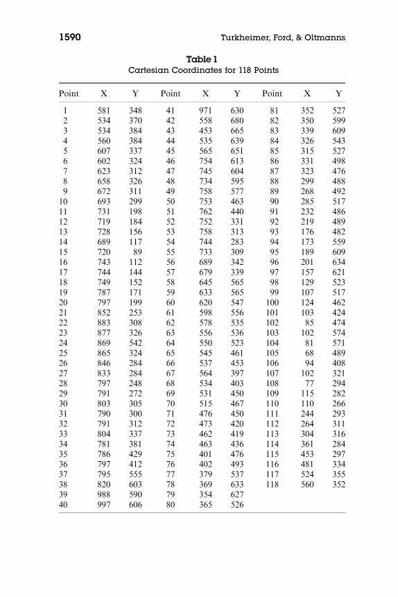
Table 1Cartesian Coordinates for 118 Points

Point X Y Point X Y Point X Y

1 581 348 41 971 630 81 352 5272 534 370 42 558 680 82 350 5993 534 384 43 453 665 83 339 6094 560 384 44 535 639 84 326 5435 607 337 45 565 651 85 315 5276 602 324 46 754 613 86 331 4987 623 312 47 745 604 87 323 4768 658 326 48 734 595 88 299 4889 672 311 49 758 577 89 268 49210 693 299 50 753 463 90 285 51711 731 198 51 762 440 91 232 48612 719 184 52 752 331 92 219 48913 728 156 53 758 313 93 176 48214 689 117 54 744 283 94 173 55915 720 89 55 733 309 95 189 60916 743 112 56 689 342 96 201 63417 744 144 57 679 339 97 157 62118 749 152 58 645 565 98 129 52319 787 171 59 633 565 99 107 51720 797 199 60 620 547 100 124 46221 852 253 61 598 556 101 103 42422 883 308 62 578 535 102 85 47423 877 326 63 556 536 103 102 57424 869 542 64 550 523 104 81 57125 865 324 65 545 461 105 68 48926 846 284 66 537 453 106 94 40827 833 284 67 564 397 107 102 32128 797 248 68 534 403 108 77 29429 791 272 69 531 450 109 115 28230 803 305 70 515 467 110 110 26631 790 300 71 476 450 111 244 29332 791 312 72 473 420 112 264 31133 804 337 73 462 419 113 304 31634 781 381 74 463 436 114 361 28435 786 429 75 401 476 115 453 29736 797 412 76 402 493 116 481 33437 795 555 77 379 537 117 524 35538 820 603 78 369 633 118 560 35239 988 590 79 354 62740 997 606 80 365 526


fectly adequate. But what does this set of points represent? Noticethat the configural information comprises more than the simple sum

of the information contained in each of the points, requiring in ad-dition the relation of the points to each other. The answer, given inFigure 2, would take a long time to figure out, given only the nu-

merical data. Numerical coordinate systems are good at reproducingdata; configural systems are good for understanding their structure.

The Curse of Dimensionality

The curse of dimensionality, which refers to the exponential rise in

complexity associated with increased dimensionality of maps, is theessential reason why interpretation of multivariate spaces is as diffi-

cult as it is. The curse takes many forms (Hastie, Tibshirani, &Friedman, 2001). Consider Figure 3, in which 100 points are dis-

tributed across spaces of one, two, and three dimensions. In a singledimension, obviously, they are only .01 units apart. If these pointswere, for example, personality items, they would provide good ‘‘cov-

erage’’ of the space defined by the single dimension. When the pointsare distributed in two dimensions, they are .1 units apart, with one

point for each of 100 squares making up the two-dimensional space.In general, if k points are uniformly distributed in p-dimensional

multidimensional space with a hypervolume of unity, the distancebetween neighboring points is given by

80060040020000

100

200

300

400

500

600

X

Y

Figure 2Configural representation of the points in Table 1.


1

k1p

ð0:1Þ

By the time you reach seven dimensions, the distance between neigh-

boring points is more than half the total width of the space. Even infour dimensions, 10,000,000 points would be required to maintain

the separation of .01 that was obtained with 100 points in a singledimension. Mentioning the possibility of four dimensions reminds us

that the curse of dimensionality is reflected in severe problems ofvisualization as well. Four dimensions are practically impossible for

the human mind to visualize, and as we will see, three dimensions aremore difficult than one might think.

Extensibility to high-dimensional spaces is one advantage of di-mensional coordinate systems for representing maps. In terms ofsimple reproducibility of data, it is no more difficult to represent

points in high dimensionality than it is in two, whereas the advantageof graphical systems for understanding configural properties be-

comes more difficult to realize in three dimensions and evaporatesquickly after that. It is important to bear in mind, however, that

although dimensional coordinate systems solve certain mathematicalaspects of representing complex dimensional spaces, they are not a

Figure 3Illustration of the curse of dimensionality in one, two, and three

dimensions.


panacea for the curse of dimensionality. They do not, for example,

help with the coverage problem, which is not a problem of repro-ducibility at all. And the shortcomings of coordinate systems for

representing the configural properties of multidimensional spaces areonly compounded in high dimensionality.

Multivariate Personality Theory as a Problem in Map

Interpretation

This entire section follows closely fromMaraun (1997). In the typical

multivariate study of individual differences in personality, responsesto a set of personality items are obtained from a large sample, usu-

ally via self-report. A covariance matrix is computed among theitems, which is then submitted to some kind of multivariate statis-

tical procedure such as factor analysis (FA). Describing the processas generally as possible, it can be divided into a sequence of steps:

� Estimation of a similarity or dissimilarity matrix among the items

� Determination of an appropriate reduced dimensionality forthis matrix

� Mapping of the location of the items in this reduced space

� Characterization of the mapping using some form ofgraphical, configural, or coordinate system

� Application of the mapping to obtain multivariate scores forthe subjects

Each step in this sequence can be undertaken in many different ways,but a particular set of choices has become dominant in the contem-

porary personality literature. The similarity matrix is computed as acovariance or correlation matrix among the items; the dimension-

ality of the space is determined by examination of the eigenvalues ofthe matrix; factor analysis is used to provide an initial configuration

of points in the reduced space; the mapping is characterized dimen-sionally, using a coordinate system based on rotation to a criterioncalled simple structure. Small loadings of items on the rotated fac-

tors are set to zero, and subject scores are obtained either throughformal estimation of factor scores or as unweighted sums of items

that load on the rotated factors.These procedures have become so universally adopted that it is now

mostly forgotten that they were once the topic of intense debate amongthe finest multivariate statisticians of the middle of the twentieth


century. A theory of multivariate analysis originating with Louis

Guttman offers an alternative route through this sequence of meth-odological choices. Although the theoretical alternatives proposed by

Guttman have been well described by Guttman and his followersand have recently been clearly reiterated in the personality domain

(Maraun, 1997), it will be necessary to outline them briefly, especiallyto establish which differences we think are particularly important.

From the outset, Guttman conceives of the problem more literallyin terms of mapping, as opposed to the numerical orientation in

terms of matrix decomposition emphasized by factor-analytic ap-proaches. Given a matrix of dissimilarities among a set of items, howcan one best locate points in a k-dimensional space so the distance

between the points (the distance metric to be employed is anothermethodological choice that needs to be made) corresponds to the

dissimilarity matrix among the items? This problem is familiar tomodern researchers as multidimensional scaling (MDS), which is the

way we will refer to it here; Guttman’s computational procedure wascalled smallest space analysis.

Guttman’s (1955) seminal contribution was to establish that FAand MDS represent alternate paths through the set of methodolog-ical choices outlined above and, furthermore, that MDS is the more

general of the two. In FA, the similarity matrix is a covariance ma-trix; in MDS it can be almost any estimate of pairwise difference,

including an inverted (to change it from a similarity to a dissimilaritymatrix) covariance matrix, a matrix based on some other statistical

estimate of distance (such as a rank correlation, or Guttman’s un-derused coefficient of monotonicity, called mu) or human judgments

of pairwise differences among stimuli. In FA, items are mapped intospace in a way that the angle between their polar coordinates cor-

responds linearly to their observed similarity; in MDS, items aremapped into space so the Euclidean distance (other distance metricscan be used) between them corresponds to their observed dissimi-

larity. In the nonmetric variety of MDS favored by Guttman, thecorrespondence between mapped distance and observed dissimilarity

is not constrained to be linear, but merely monotonic.Although we are convinced by Guttman’s argument that the

MDS procedures for locating points in reduced dimensional spacesoffer many advantages over FA procedures, we also agree with

Maraun (1997) that these differences are not at the crux of the mat-ter. At this point in the methodological sequence, FA andMDS have


used different methods to accomplish the same thing: Points have

been located in a reduced dimensional space in a way that maximizessome criterion of correspondence between the distances among the

points and the similarities among the items. From here forward, theproblem for either FA or MDS is to characterize the multivariate

map that has resulted.In FA, the near-universal procedure is to select a coordinate system

using a criterion called ‘‘simple structure’’ (Thurstone, 1947), whichentails finding coordinates that maximize the loadings of the items on

one dimension and minimize them on the others, amounting to find-ing axes that lie as close to the points as possible. Rotation to simplestructure has become so commonplace, and the computational meth-

ods to conduct it so easy to use, that several important considerationshave been widely forgotten. First of all, notwithstanding the simple

structure criterion, the location of the coordinate axes through amultivariate space is MBA. From a mathematical point of view, no set

of axes is any better than another (Mulaik, 2005; Sternberg, 1977;Thurstone, 1947). The simple structure criterion is a matter of human

computational convenience rather than a structural property of thedata. One must therefore be very careful about attributing a substan-tive interpretation to any particular rotation of the coordinate axes.

Second, the fit of the data to the simple structure criterion is not agiven but is rather an empirical hypothesis about the multivariate

map. Many maps, indeed most maps, do not have simple structure.(The mountains in Virginia, for example, lack simple structure in that

their location is not conveniently described by a set of coordinateaxes.) Personality data in particular have repeatedly been shown to

lack simple structure (Church and Burke, 1994; McCrae, Zonderman,Costa, Bond, & Paunonen, 1996). The common practice of setting

small loadings to zero after axes have been rotated (or even worse,dropping items that ‘‘cross-load’’ on more than one factor) amountsto imposing simple structure on a map by eliminating the inconvenient

parts of the data that fail to fit the model.The classic example of the failure of dimensional coordinate sys-

tems to capture the important structural properties of a psycholog-ical phenomenon is Shepard’s color perception data (1978), and

in this case we refer the reader to Maraun’s detailed account. Tosummarize, Shepard reanalyzed judgments of similarity among 14

color samples, submitted the dissimilarity matrix to an MDS proce-dure, and found that the resulting configuration of colors formed a


circle, a similarity structure called a circumplex by Guttman. The

circumplex reveals the structure of similarities among the colors butdoes not conform to simple structure. Factor analyses of the same

data matrix resulted in five orthogonal dimensions that completelymissed the essential circumplexical structure of the data.

The Circumplex in Personality Theory

The prominent dimensional system known as the Five-Factor Model

(FFM; Goldberg, 1990; McCrae & Costa, 1990) of personality hasemerged out of traditional FA (Cattell, 1957). Its development was

achieved using the lexical hypothesis, the proposition that individualdifferences in personality become encoded in the everyday vocabu-lary. Factor analyses of self- and peer-ascription of adjectival

descriptors, many derived from the compilation of Allport and Od-bert (1936), resulted in a diversity of factor theories that eventually

converged on the FFM outlined by McCrae and Costa (1990). Al-though the FFM is unquestionably one of the most significant per-

sonality research discoveries in recent history, an alternativetradition (Leary, 1957; Kiesler, 1983; Wiggins, 1982) has analyzed

a subset of Allport and Odbert’s adjectives that were interpersonal innature and demonstrated that these data exhibited a circumplexstructure as well.

Circumplexical models of normal personality have also been ap-plied to the personality disorders (Blashfield, Sprock, Pinkston, &

Hodgin, 1985; Pincus & Gurtman, 2006; Soldz, Budman, Demby, &Merry, 1993; Widiger & Hagemoser, 1997; Wiggins & Pincus, 1989).

The circumplexical solutions that have been reported have differedin detail but are similar in overall structure. Following Wiggins and

colleagues, the circumplex is usually described in terms of octants.Proceeding from the (MBA) top, they are, Dominance, Extraver-

sion, Warmth, Ingenuous, Submissive, Aloof, Cold, and Arrogant(see, e.g., Figure 4.4 in Wiggins, 1996). Several shortcomings of theextant literature will be addressed in the current article. First, all

studies reported to date have been based on preexisting PD scalescores rather than on the individual items. Our analysis will show

that existing PD scales do not necessarily correspond to the simi-larity structure of the items.

Second, previous reports have been limited to circumplexical rep-resentations in the plane, although many published solutions are


obviously not circumplexical. This is particularly true because the

solutions often do not form a hollow circle but rather a filled-in disk,which, as we will see, is known as a radex (e.g., Soldz et al., 1993).

We find that the radex structure has an important interpretation,and, moreover, that two dimensions are inadequate to represent PD

data, leading us to explore solutions in three. Existing circumplexicalmodels that attempt to describe personality data in greater than two

dimensions have consisted of multiple orthogonal circumplexes (DeRaad & Hofstee, 1993). Although this approach succeeds in dem-

onstrating that the dimensional and circumplexical approaches tomultivariate structure are not necessarily at odds with each other,orthogonal circumplexes share many of the disadvantages of or-

thogonal dimensions for the description of multivariate structure.Returning to our geographic metaphor, describing multivariate

space with orthogonal circumplexes is like describing earthly geog-raphy only via reference to the ‘‘circumplexes’’ known as the equator

and the Greenwich Meridian. Like latitude and longitude applied totwo-dimensional maps, spherical coordinates are mathematically

sufficient but not necessary and have significant limitations as toolsfor representing geographical structure.

In summary: (1) Although MDS offers some important advantages

over FA as a tool for the representation of complex data in reduceddimensionality, the choice between statistical procedures is not crucial

to our case. FA and MDS both represent stimuli in reduced multidi-mensional space, and the important question is how their configura-

tion in space is to be characterized. (2) Coordinate systems rotated tosimple structure are a poor representation of many maps. (3) Even in

maps that do show some degree of simple structure, dimensional co-ordinate systems are not particularly informative about their config-

ural properties. (4) Dimensional coordinates rotated to simplestructure, like any concrete system for map characterization, areMBA. This last point is not unique to coordinate systems since the

same is true of any alternative that might be proposed. Rather, it con-tradicts the now-widespread belief that dimensional coordinate sys-

tems rotated to simple structure have some special claim on the actualstructural properties of the phenomenon under study. They do not.

In the current article we apply regional interpretation of multidi-mensional scaling analyses to the structure of personality disorder

symptoms, using a large sample of self-report data. Although severalinteresting aspects of the structure of personality disorders are illumi-


nated by a careful interpretation of a two-dimensional model, we find

that a three-dimensional model provides a substantially better fit. Wethen explore some of the considerable difficulties that are encountered

in the attempt to perform regional interpretation in three dimensions.

METHOD

Participants

The Multisource Assessment of Personality Pathology (MAPP) wasadministered to two samples.

Sample 1

This sample consisted of 1562 Air Force recruits (60% male, 40% female)who had just completed basic training at Lackland Air Force Base in SanAntonio, Texas. Participants were general enlisted personnel who, uponarrival for 6 weeks of basic training, were grouped together to form unitscalled flights. Unit sizes ranged from 27 to 54 recruits per flight (M5 41,SD5 6.3) and were either same-sex or mixed-sex in composition. Thesample comprised 64% Caucasians, 17% African Americans, 9% His-panics, and 10% other ethnicities (Asian, Native American, or biracial)with ages ranging from 18 to 35 and a mean of 20.2 years (SD5 2.4).Participation in the study was voluntary.

Sample 2

This sample consisted of 1693 college freshmen (33% male, 67% female)attending the University of Virginia. Participants were grouped by thesame-sex dormitory hall on which they lived together during the first se-mester of the academic year. Each group was then assessed during thefollowing spring term. Group sizes ranged from 3 to 21 students (M5 13,SD5 3.4). Participants were 79% Caucasian, 8% Asian, 6% AfricanAmerican, and 7% other ethnicities (Hispanic, Native American, or bi-racial) with ages ranging from 18 to 27 (M5 18.6, SD5 0.25). For par-ticipation, the students received their choice of experiment credit towardsa psychology course or monetary compensation.

Measures

Multisource Assessment of Personality Pathology (MAPP)

The MAPP, a personality assessment inventory primarily used as aresearch instrument in the Peer Nomination Project (Oltmanns &


Turkheimer, 2006), consists of 103 items, including 78 that are transla-tions of the DSM-IV (1994) diagnostic criteria for each of the 10 PDs intolay terms (See Table 2). These items were constructed by simplifying theDSM-IV criteria to capture their meaning while eliminating any psycho-logical jargon. One of the criteria for Narcissistic PD, ‘‘Is often envious ofothers or believes that others are envious of him or her (DSM-IV-TR, p.717),’’ was split into two separate items: ‘‘Is jealous of other people,’’ and‘‘Thinks other people are jealous of him/her.’’ Expert consultants in AxisII psychopathology then reviewed the translations and revised them foraccuracy and clarity. The remaining 24 items describe positive character-istics, such as ‘‘Is sympathetic and kind to others’’ or ‘‘Has a cheerful andoptimistic outlook on life.’’ These were included to decrease the emphasison pathological personality traits. Only the 78 PD items were used in thecurrent analysis.

Procedure

As part of a larger study investigating the utility of peer report inpersonality assessment, participants were screened using a computerizedbattery of measures. Included in these measures was the self-reportportion of the MAPP. Each participant was asked to rate him- or her-self on a 4-point scale: (0) Never this way, (1) Sometimes this way, (2)Usually this way, (3) Always this way. Completion of this measuretypically ranged from 45 minutes to 1 hour of the total 2 hours ofassessment time.

Statistical Procedures

Guttman’s Monotonicity Coefficient (Raveh, 1978), m, was used to esti-mate the similarities among the 78 PD items of the MAPP. The m coeffi-cient is a measure of the degree to which the relation between a pairof variables is monotonic, i.e., an increase in the value of one variableis associated with an increase in the value of the other, without assum-ing linearity of the relation. The magnitudes of these coefficientscan range from � 1 to 1, where m5 1 describes a perfect positive mono-tonic relationship between the two items. Mu was computed using theformula,

m1 ¼

Pi> j

Yi � Yj

� �Pi> j

Yi � Yj

�� 1 � j < i � N ð1:2Þ

where Yi�Yj refers to the observed difference between the ith and jth

items and N is the total number of items in the scale, that is, 78.


Table 2Multi-Source Assessment of Personality Pathology PD Items

Item PD DSM-IV Criterion

8 SZ A29 ST A2

11 BD 712 NA 213 AV 514 DP 215 OC 219 ST A720 AS A221 HS 323 NA 424 AV 425 DP 826 OC 828 PA A229 SZ A130 ST A931 AS A332 BD 633 HS 534 NA 935 AV 636 DP 737 OC 739 PA A340 SZ A441 ST A642 AS A643 BD 244 BD 545 HS 646 NA 747 AV 748 DP 649 OC 652 PA A453 SZ/ST A5/A854 ST A455 AS A456 AS A7

(Continued)


The similarity matrix was then submitted to nonmetric multidimen-sional scaling (NMDS) to recover a spatial representation of the itemsbased on the rank order of the similarities. This analysis was carried outusing the SAS System’s PROC MDS, which requires the values of the

Table 2 (Cont.)

Item PD DSM-IV Criterion

57 BD 858 HS 759 NA 860 AV 361 DP 362 OC 565 SZ A766 AS A167 BD 168 BD 969 HS 870 NA 571 AV 172 DP 173 DP 474 OC 177 PA A678 SZ A679 ST A980 AS A581 HS 182 AV 283 DP 584 OC 387 PA A188 ST A389 BD 490 HS 291 NA 192 OC 495 PA A796 HS 497 NA 3100 ST A5101 NA 6102 PA A5103 NA 8


similarities to be positive. To accommodate this constraint, a value of 1was added to the monotonicity coefficients to shift their values from 0 to2, where zero describes a perfect ‘‘negative’’ monotonic relationship. Fitof the NMDS solution was assessed with a goodness-of-fit index calledStress Formula 1 (Kruskal & Carroll, 1969).

Stress ¼

ffiffiffiffiffiffiffiffiffiffiffiffiffiffiffiffiffiffiffiffiffiffiffiffiffiffiffiffiffiffiffiffiffiPðf ðxijÞ � dijÞ2P

d2ij

sð1:3Þ

In the equation, xij are observed pairwise differences, transformed by amonotonic function, f(xij); dij represents the Euclidean distance betweenpoints i and j in the estimated solution. The implication of the monotonictransform f is that only the ordinal properties of the observed distancesare being modeled, creating an analysis known as nonmetric multidimen-sional scaling. Models in which the observed distances are modeled di-rectly are known as metric scaling. Solutions with stress values less than0.20 were considered to reflect acceptable goodness-of-fit as suggested byKruskal (1964).

RESULTS

Two-Dimensional Solution

The values of m ranged from � 0.27 to 0.91. Using the transformed mcoefficients as input, NMDS produced stress values of 0.21, 0.15,

and 0.12 for the two-, three-, and four-dimensional solutions, re-spectively, indicating that the three- and four-dimensional solutions

fall in the acceptable range. Although the fit in two dimensions wasinadequate, this solution was interpreted anyway to provide a basis

for the understanding of a subsequent three-dimensional model.Examination of the overall structure of the configuration revealed

that it is best described as a radex, a structure first described byGuttman, 1954 (Figure 4). It may be that the failure of Guttman-

style interpretation of multivariate spaces can be attributed to thesuperficially unimpressive appearance of a radex, which looks sus-piciously like a scatterplot of the relation between two variables that

have turned out to be uncorrelated. In fact, the radex is highlystructured. It consists of two components—a circular dimension

called a circumplex and an inner-outer dimension running from thecenter of the configuration to the perimeter, called a simplex.

To follow our interpretation of the solution that follows, it will beimportant to understand the details of the mapping of the radex


structure onto the pairwise item similarities. Recall that the NMDS

solution is a literal representation of inter-item similarity. Aroundthe periphery of the solution, items are close to those around them

but far away from equally peripheral items on the other side of theconfiguration. For example, Item 24 is estimated to be very similar to

Item 61 but quite dissimilar to Item 78. In contrast, items near thecenter of the configuration are estimated to be roughly equal in sim-

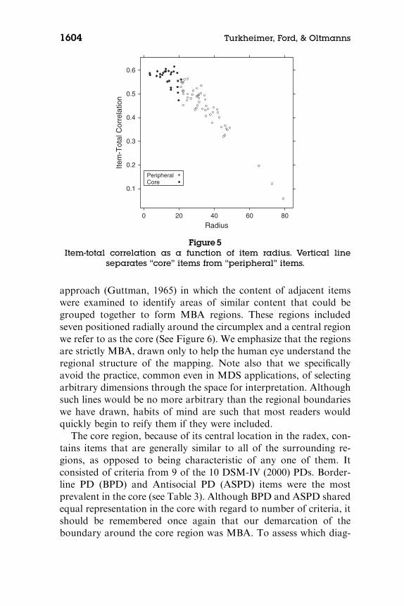
ilarity to items around the perimeter of the circumplex. These items,therefore, are more globally typical of the entire domain, rather thanbeing specific to a particular region. To illustrate this property, we

computed the corrected item-total correlations (the correlation ofeach item with the total of the other items) and plotted them against

the distance between the modeled location of each item and the cen-ter of the solution. The result is shown in Figure 5. The core items

are more broadly representative of the overall tendency to self-reportAxis-II symptoms.

The radex produced by the two-dimensional solution was given apreliminary interpretation using a neighborhood or regionalization

Figure 4Two-dimensional radex NMDS solution of MAPP PD items.


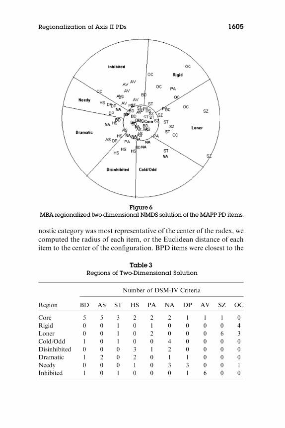
approach (Guttman, 1965) in which the content of adjacent itemswere examined to identify areas of similar content that could be

grouped together to form MBA regions. These regions includedseven positioned radially around the circumplex and a central region

we refer to as the core (See Figure 6). We emphasize that the regionsare strictly MBA, drawn only to help the human eye understand the

regional structure of the mapping. Note also that we specificallyavoid the practice, common even in MDS applications, of selecting

arbitrary dimensions through the space for interpretation. Althoughsuch lines would be no more arbitrary than the regional boundaries

we have drawn, habits of mind are such that most readers wouldquickly begin to reify them if they were included.

The core region, because of its central location in the radex, con-

tains items that are generally similar to all of the surrounding re-gions, as opposed to being characteristic of any one of them. It

consisted of criteria from 9 of the 10 DSM-IV (2000) PDs. Border-line PD (BPD) and Antisocial PD (ASPD) items were the most

prevalent in the core (see Table 3). Although BPD and ASPD sharedequal representation in the core with regard to number of criteria, it

should be remembered once again that our demarcation of theboundary around the core region was MBA. To assess which diag-

Radius

Item

-Tot

al C

orre

latio

n

0.1

0.2

0.3

0.4

0.5

0.6

0 20 40 60 80

PeripheralCore

Figure 5Item-total correlation as a function of item radius. Vertical line

separates ‘‘core’’ items from ‘‘peripheral’’ items.


nostic category was most representative of the center of the radex, we

computed the radius of each item, or the Euclidean distance of eachitem to the center of the configuration. BPD items were closest to the

Figure 6MBA regionalized two-dimensional NMDS solution of the MAPP PD items.

Table 3Regions of Two-Dimensional Solution

Region

Number of DSM-IV Criteria

BD AS ST HS PA NA DP AV SZ OC

Core 5 5 3 2 2 2 1 1 1 0

Rigid 0 0 1 0 1 0 0 0 0 4

Loner 0 0 1 0 2 0 0 0 6 3

Cold/Odd 1 0 1 0 0 4 0 0 0 0

Disinhibited 0 0 0 3 1 2 0 0 0 0

Dramatic 1 2 0 2 0 1 1 0 0 0

Needy 0 0 0 1 0 3 3 0 0 1

Inhibited 1 0 1 0 0 0 1 6 0 0


center, followed by Schizotypal and Antisocial (Table 4). The criteriafor obsessive-compulsive PD were the furthest from the center of the

configuration, suggesting that the OC criteria are the least charac-teristic of the overall domain of Axis II criteria. We will interpret thestructure of the regions in more detail as we proceed to the three-

dimensional solution.To compare the NMDS solution to a traditional simple structure

solution derived from factor analysis, an exploratory factor analysisof the 78 MAPP items was performed using M Plus. The number of

factors needed to represent the MAPP was determined using theKaiser-Guttman criterion of considering factors that have eigenval-

ues greater than 1.0 and by considering factor interpretability.Model fit was gauged by the Root Mean Square Error of Approx-

imation (RMSEA) statistic where an RMSEA less than 0.05 isconsidered acceptable (Browne & Cudeck, 1993). Using these con-siderations a five factor solution was accepted as showing both good

model fit (RMSEA5 0.03) and interpretability.Interpretation of the factor loadings was conducted following a

Promax rotation of the original factor solution. The correlationsamong the factors in this analysis were found to be small to mod-

erate, ranging from 0.23 to 0.49 (see Table 5). A loading cut of.30 was used for inclusion of an item in interpretation of a factor;

consequentially 6 of the 78 items failed to be included in any of thefive factors as seen in Table 6. Inspection of the content of the items

Table 4Mean Distance of PDs From Center of Two-Dimensional Solution

PD Mean Radius

Borderline 14.79

Schizotypal 18.93

Antisocial 19.08

Paranoid 22.42

Dependent 25.27

Narcissistic 26.19

Avoidant 28.64

Histrionic 28.79

Schizoid 36.55

Obsessive-compulsive 46.37


with the highest loadings on each of the factors resulted in the fol-

lowing labels: Unrestrained, Dependent, Reckless, Rigid/Loner, andIdentity Problems.

Based on the factor-analytic solution, the items composing eachfactor were located in the NMDS derived space. Upon visual in-

spection, the items associated with a given factor were found togroup together in a reasonably contiguous manner as illustrated in

Figure 7. The factor-based regions are simply another MBA region-alization of the two-dimensional NMDS space, reasonable enoughon its own terms, but with no special claim to the ‘‘true’’ multivariate

structure of the data.To quantify the amount of information lost by discarding items

with factor loadings that did not meet the 0.3 cutoff we performed ananalysis proposed by Maraun (1997). Maraun pointed out that since

all of the factor loadings are required to represent the configurationof the items, removing loadings in order to impose very simple

Table 5Correlations Among the Five Promax Rotated Factors

Factor Unrestrained Dependent Reckless Rigid/Loner ID Problems

Unrestrained –

Dependent 0.41 –

Reckless 0.40 0.30 –

Rigid/Loner 0.30 0.30 0.23 –

ID Problems 0.49 0.43 0.41 0.40 –

Table 6Loadings of a Five Factor Solution of the MAPP

Item

Factors

Unrestrained Dependent Reckless Rigid/Loner ID Problems h2

8 � 0.06 � 0.23 � 0.10 0.48 0.25 0.36

9 0.09 0.05 0.05 � 0.04 0.39 0.17

11 � 0.20 0.27 0.01 0.12 0.59 0.48

12 0.41 0.03 0.02 0.09 0.23 0.23

13 � 0.25 0.54 � 0.05 0.22 0.25 0.47

(Continued)


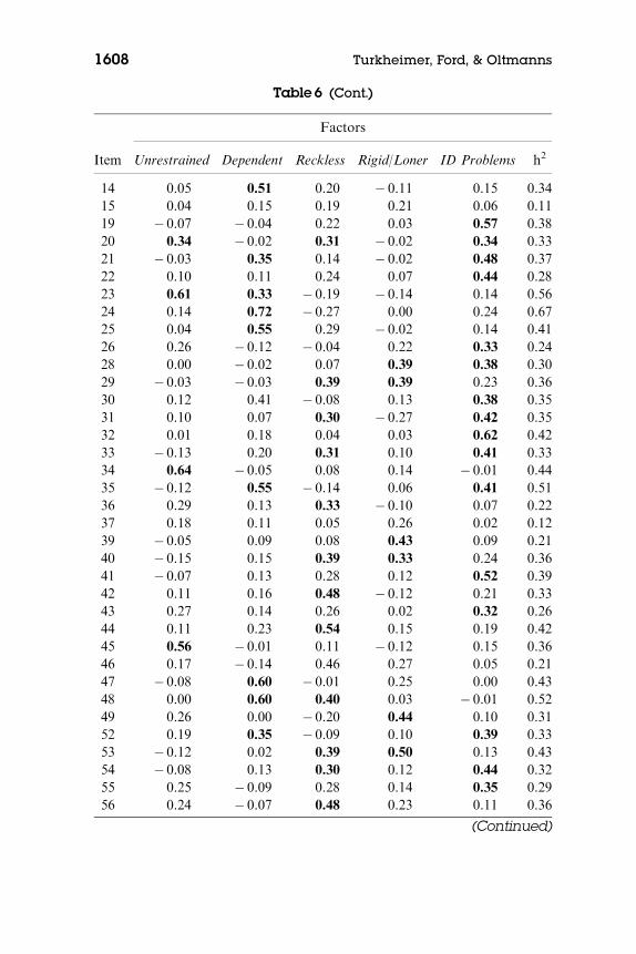
Table 6 (Cont.)

Item

Factors


14 0.05 0.51 0.20 � 0.11 0.15 0.34

15 0.04 0.15 0.19 0.21 0.06 0.11

19 � 0.07 � 0.04 0.22 0.03 0.57 0.38

20 0.34 � 0.02 0.31 � 0.02 0.34 0.33

21 � 0.03 0.35 0.14 � 0.02 0.48 0.37

22 0.10 0.11 0.24 0.07 0.44 0.28

23 0.61 0.33 � 0.19 � 0.14 0.14 0.56

24 0.14 0.72 � 0.27 0.00 0.24 0.67

25 0.04 0.55 0.29 � 0.02 0.14 0.41

26 0.26 � 0.12 � 0.04 0.22 0.33 0.24

28 0.00 � 0.02 0.07 0.39 0.38 0.30

29 � 0.03 � 0.03 0.39 0.39 0.23 0.36

30 0.12 0.41 � 0.08 0.13 0.38 0.35

31 0.10 0.07 0.30 � 0.27 0.42 0.35

32 0.01 0.18 0.04 0.03 0.62 0.42

33 � 0.13 0.20 0.31 0.10 0.41 0.33

34 0.64 � 0.05 0.08 0.14 � 0.01 0.44

35 � 0.12 0.55 � 0.14 0.06 0.41 0.51

36 0.29 0.13 0.33 � 0.10 0.07 0.22

37 0.18 0.11 0.05 0.26 0.02 0.12

39 � 0.05 0.09 0.08 0.43 0.09 0.21

40 � 0.15 0.15 0.39 0.33 0.24 0.36

41 � 0.07 0.13 0.28 0.12 0.52 0.39

42 0.11 0.16 0.48 � 0.12 0.21 0.33

43 0.27 0.14 0.26 0.02 0.32 0.26

44 0.11 0.23 0.54 0.15 0.19 0.42

45 0.56 � 0.01 0.11 � 0.12 0.15 0.36

46 0.17 � 0.14 0.46 0.27 0.05 0.21

47 � 0.08 0.60 � 0.01 0.25 0.00 0.43

48 0.00 0.60 0.40 0.03 � 0.01 0.52

49 0.26 0.00 � 0.20 0.44 0.10 0.31

52 0.19 0.35 � 0.09 0.10 0.39 0.33

53 � 0.12 0.02 0.39 0.50 0.13 0.43

54 � 0.08 0.13 0.30 0.12 0.44 0.32

55 0.25 � 0.09 0.28 0.14 0.35 0.29

56 0.24 � 0.07 0.48 0.23 0.11 0.36

(Continued)


Table 6 (Cont.)

Item

Factors


57 0.19 � 0.06 0.35 0.17 0.36 0.32

58 0.10 0.65 0.04 � 0.10 � 0.01 0.44

59 0.67 0.08 0.17 0.08 � 0.10 0.50

60 � 0.03 0.51 0.11 0.33 0.06 0.39

61 0.02 0.69 0.04 0.11 0.01 0.49

62 0.11 0.33 � 0.02 � 0.03 0.14 0.14

65 0.02 � 0.22 0.35 0.48 0.19 0.44

66 0.28 � 0.11 0.62 0.03 0.08 0.48

67 0.09 0.47 0.46 � 0.02 � 0.10 0.45

68 0.13 0.27 0.14 0.01 0.42 0.29

69 0.23 0.29 0.22 0.04 0.06 0.20

70 0.59 0.05 0.28 0.16 � 0.13 0.47

71 0.04 0.37 0.27 0.32 0.08 0.32

72 0.08 0.61 0.13 � 0.05 0.01 0.40

73 0.02 0.69 0.25 � 0.03 � 0.08 0.55

74 0.13 0.31 � 0.07 0.45 � 0.18 0.35

77 0.27 0.14 0.18 0.21 0.24 0.23

78 0.05 � 0.34 0.16 0.21 0.04 0.19

79 � 0.08 0.24 0.18 0.42 0.21 0.32

80 0.26 � 0.06 0.54 0.03 0.19 0.40

81 0.65 0.12 0.07 � 0.06 0.04 0.45

82 0.18 0.51 0.03 0.15 0.06 0.32

83 0.22 0.32 0.53 0.09 � 0.05 0.44

84 � 0.01 0.10 0.30 0.54 � 0.09 0.40

87 0.08 0.22 0.13 0.35 0.23 0.25

88 0.01 0.00 0.18 0.18 0.42 0.24

89 0.26 � 0.16 0.52 � 0.12 0.27 0.45

90 0.41 � 0.09 0.46 � 0.07 0.02 0.39

91 0.68 � 0.05 0.25 0.15 � 0.10 0.56

92 0.12 0.07 � 0.10 0.37 � 0.21 0.21

95 0.20 0.07 0.34 0.08 0.09 0.18

96 0.70 0.04 0.06 � 0.08 � 0.09 0.51

97 0.63 0.04 0.29 0.13 � 0.17 0.53

100 0.06 0.33 0.07 0.23 0.33 0.28

101 0.37 0.08 0.47 0.11 0.05 0.38

102 0.27 0.10 0.03 0.16 0.24 0.17

103 0.37 0.49 � 0.12 0.00 0.15 0.41


structure results in a loss of information. To quantify this loss, which

Maraun called the percentage of structure ignored, the sums ofsquares of the factor loadings less than the cut score are divided

by the total sum of squares of all factor loadings. Application of thismethod to our FA result showed that 23% of the structure was ig-

nored by choosing only to interpret factor loadings greater than thecutoff.

Three-Dimensional Solution

As we have already noted, the two-dimensional NMDS model doesnot meet conventional fit criteria. We suspect that this is not an un-

common outcome, and the difficulties we encounter in the regionalinterpretation of the three-dimensional solution may suggest why

most MDS analyses of personality data stop at two dimensions de-spite marginal fit. Modern computer graphics offer many advantages

Figure 7Two-dimensional NMDS solution. Numbers correspond to factors

from Promax rotation of FA with five factors: 1 = Unrestrained,2 = Dependent, 3 = Reckless, 4 = Rigid/Loner, 5 = ID Problems.


in the visualization of three-dimensional data, and we think we

achieve some success in what follows, although in a journal formatwe are also hamstrung by the constraints of static grayscale images.

We began our interpretation of the three-dimensional NMDS bycomparing it to the two-dimensional result. To facilitate comparison,

a procrustes rotation was applied to the coordinates produced by thethree-dimensional solution, with a criterion of rotating the first two

dimensions of the 3-D solution to conform as closely as possible tothe two-dimensional solution, with the third dimension orthogonal

to the first two (see Figure 8). Aligning the solution in this manneremphasizes the additional information that is provided by the thirddimension. Despite the attempt to make the relationship between the

two- and three-dimensional solutions more apparent, however, theproblem of regionalization, which was a matter of straightforward

intuition in two dimensions, becomes much more difficult in three.The task is now to divide three-dimensional space into ‘‘chunks’’

that regionalize space in the same way that outlined areas regionalizethe plane. The eye has a hard time following and making sense of the

spatial relationships among the items once they are arrayed in threedimensions.

Figure 8Procrustes rotated three-dimensional NMDS solution. First two dimen-

sions correspond as closely as possible to two-dimensional solution,with new third dimension orthogonal.


In order to solve this problem in multidimensional data visual-

ization, we relied on our knowledge of the structure of the similarityspace in two dimensions: a core region containing items that weremoderately similar to all other items, surrounded by a circumplex of

items that were highly similar to their neighbors but different fromthose on the other side of the circumplex. With this in mind, we

simplified the three-dimensional configuration into two structures, acore and a spherex. The core region was specified using the third of

the items that were closest to the centroid of the three-dimensionalconfiguration. The coordinates of the remaining items were pro-

jected to the surface of a unit sphere (see Figure 9).We then attempted to characterize the regional structure of the

core and the spherex. The relatively smaller number of items in thecore could be regionalized in terms of four three-dimensional re-gions: Suspiciousness, Anger, Isolation, and Identity problems. This

core configuration is illustrated in Figure 10. Once the noncore itemshave been projected outward to the spherex, the problem becomes

one of identifying MBA regions on the surface of a globe. The itemcontent of adjacent items on the sphere was examined for similarity

and separated as before to form eight regions as illustrated in Figure9. These regions are very similar to those defined in the two-dimen-

sional solution except for the emergence of a Schizotypy region atthe northern polar cap (with MBA orientation!) of the sphere.

Figure 9Regionalized MAPP PD items on the surface of the sphere.


DISCUSSION

When stimuli of high dimensionality are submitted to a multivariate

statistical procedure that maps them into a lower dimensionality,characteristics of the data fix two aspects of the result—its dimen-sionality and its structure. Although, in our view, applied data gen-

erally do not have a ‘‘true’’ dimensionality that can be ascertained bythe researcher, the fit of a model in any given reduced dimensionality

is, nevertheless, strictly a characteristic of the data themselves. By the‘‘structure’’ of the data we refer to their shape or configuration in the

multidimensional space that is chosen. Once again, applied data areunlikely to result in a perfectly circular configuration, and it is up to

the researcher to decide whether a given configuration is closeenough to a perfect circumplex to ignore the differences. The shape

of the locations of the items in the reduced space, however, is de-termined by the multivariate structure of the data.

Figure 10MBA structure of core the three-dimensional NMDS solution. Lines aredrawn to help visualize four three dimensional regions of core:suspiciousness, aggressiveness, isolation, and identity disturbance.


All subsequent interpretations of multivariate results are MBA.

The data do not militate which end of a configuration belongs ontop, leaving the investigator free to orient the configuration as he or

she wishes. This freedom can be a boon to flexible and descriptiveinterpretation of multivariate data, but it comes with the inherent

danger that the investigator will soon forget that the decision toorient the data in a particular way was a matter of convenience, not

empirical fact. Such a misguided investigator might then begin toassign empirical meaning to these orientations, like a child who

wonders whether the location of the northern hemisphere on top ofthe globe is a reflection of some inherent superiority over the south.

Our admittedly oversimplified account of Guttman’s scientific

prescription is that multivariate science should be focused resolutelyon quantification of dimensionality and interpretation of configural

structure because this is where empirical constraints on our theoriz-ing are located. The data determine how many dimensions are re-

quired to represent self-reported PD symptoms at some criterion ofaccuracy, and within that mapping the data determine the contiguity

of like to like and the configuration of the structure of the whole.Although some form of line drawing is necessary to make sense of amultidimensional mapping, all line drawing is MBA. We prefer

drawing of regions to the more common drawing of dimensions forseveral reasons. First, it serves as a corrective to the prevailing habit

of believing that dimensions defined by simple structure are a re-flection of natural laws; for whatever reason, scientists appear to be

more willing to accept regions for what they are, that is, as mean-ingful but arbitrary contingencies in the service of multidimensional

description. Second, regions are a more flexible method for opera-tionalizing the crucial concept of contiguity as a means of capturing

the location of the mountains in Virginia or the narcissism items in amapping of the MAPP. Straight lines extending from positive tonegative infinity are very limiting as a means of categorizing spatial

configurations of contiguity, especially as regards soft psychologicaldata.

Our regional investigation of the structure of the MAPP hasdemonstrated several interesting facts about the structure of the

personality disorders. The circumplexical aspect of our solution isgenerally similar to Wiggins’s version of the interpersonal circle

(1995). To provide some orientation between the two representa-tions, the Disinhibited region in our two-dimensional model can be


viewed as a blending between the vindictive and domineering octants

of the IPC. Both describe the portion of personality space made ofnarcissistic and domineering traits. Once the two models are aligned

in this way, one can continue about the circle and find fairly directcorrespondence between them based on their regional content.

Minor differences are likely to be attributable to our use of individ-ual criteria rather than predefined scales, as our analysis shows that

scales do not correspond very well to the actual locations of theitems.

Soldz et al. (1993) reported a solution that looked more like aradex than a circumplex, but they did not offer an interpretation ofthe radexical dimension. They also reported the ‘‘surprising’’ con-

clusion that Borderline PD was located close to the origin. We haveshown that the radex dimension of the solution has a clear interpre-

tation that has important implications for our understanding of per-sonality disorders: certain traits, which we have characterized as

anger, isolation, suspiciousness, and identity disturbance, are com-mon to all of the PDs in the concrete sense that they have high item-

total correlations with the universe of PD symptoms. Other traits,which can be viewed as more specialized variants of the core traits,are typical of specific types of PD but not of the universe as a whole.

From Table 7, one can see that the mu coefficients of core regionswith each of the 10 PD scales of the MAPP are generally higher

Table 7Similarities of the Three-Dimensional Regions to the 10 DSM-IV PDs

Region BD AS ST HS PA NA DP AV SZ OC

Anger Problems 0.96 0.98 0.90 0.90 0.90 0.92 0.86 0.76 0.80 0.72

Identity Problems 0.97 0.83 0.91 0.86 0.84 0.78 0.82 0.80 0.74 0.67

Isolation 0.88 0.81 0.93 0.78 0.93 0.78 0.81 0.85 0.87 0.75

Suspiciousness 0.94 0.81 0.93 0.86 0.91 0.84 0.94 0.89 0.64 0.74

Rigid 0.73 0.55 0.74 0.63 0.79 0.65 0.67 0.71 0.67 0.95

Loner 0.73 0.67 0.87 0.59 0.84 0.68 0.54 0.63 0.93 0.84

Cold/Odd 0.75 0.77 0.75 0.69 0.78 0.85 0.57 0.52 0.82 0.73

Disinhibited 0.84 0.88 0.76 0.96 0.79 0.96 0.76 0.59 0.62 0.65

Dramatic 0.89 0.92 0.79 0.95 0.76 0.91 0.90 0.75 0.55 0.64

Needy 0.83 0.71 0.73 0.84 0.73 0.78 0.96 0.86 0.38 0.73

Inhibited 0.81 0.64 0.79 0.73 0.77 0.72 0.89 1.00 0.50 0.68

Schizotypy 0.85 0.78 0.98 0.79 0.74 0.70 0.70 0.68 0.80 0.62


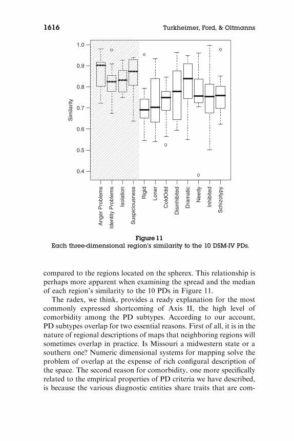
compared to the regions located on the spherex. This relationship is

perhaps more apparent when examining the spread and the medianof each region’s similarity to the 10 PDs in Figure 11.

The radex, we think, provides a ready explanation for the mostcommonly expressed shortcoming of Axis II, the high level ofcomorbidity among the PD subtypes. According to our account,

PD subtypes overlap for two essential reasons. First of all, it is in thenature of regional descriptions of maps that neighboring regions will

sometimes overlap in practice. Is Missouri a midwestern state or asouthern one? Numeric dimensional systems for mapping solve the

problem of overlap at the expense of rich configural description ofthe space. The second reason for comorbidity, one more specifically

related to the empirical properties of PD criteria we have described,is because the various diagnostic entities share traits that are com-

Ang

er P

robl

ems

Iden

tity

Pro

blem

s

Isol

atio

n

Sus

pici

ousn

ess

Rig

id

Lone

r

Col

dOdd

Dis

inhi

bite

d

Dra

mat

ic

Nee

dy

Inhi

bite

d

Sch

izot

ypy

0.4

0.5

0.6

0.7

0.8

0.9

1.0

Sim

ilarit

y

Figure 11Each three-dimensional region’s similarity to the 10 DSM-IV PDs.


mon to the entire domain. An individual who is withdrawn, hostile,and suspicious, with changeable identity, is at risk for practically anypersonality disorder, and it is no surprise that many such people

qualify for several of them. Figure 12 is a schematic representation ofhow common traits might lead to comorbidity among the PDs.

Another longstanding, if less frequently addressed, issue involvesthe special standing of Borderline PD among the personality disor-

ders. Borderline was among the first PDs to be recognized clinicallyand retains an iconic status among personality disorders. Why? In

fact, conventional psychometric and factor-analytic studies of thePDs suggest that the two main characteristics of Borderline PD,

emotional dysregulation and identity disturbance, do not seem tobelong together in the same syndrome (Thomas, Turkheimer, &Oltmanns, 2003). These conventional analyses, however, lack the

radexical concept of core traits that we have developed here. Of allthe PDs, BD symptoms lie closer to the core of the domain by a

considerable margin. Borderline PD is literally iconic: It comprisesthe traits that define the universe of PDs.

It is also important to emphasize that many other MBA region-alizations of the PD domain are possible and interesting, and indeed

might be desirable under some circumstances. For example, inFigure 6 the location of the narcissism items have been printed in

Figure 12Schematic representation of trait comorbidity, illustrating that

regional PD diagnoses can be expected to overlap because theyshare common core traits.


boldface. Although their location does not correspond very well to

the regionalization we have chosen, they nevertheless form a nearlycontiguous region of the space, and characterizing that region helps

us to understand the relation of narcissistic traits to other PD traits.Narcissism is a trait that is moderately typical of PDs in general,

running along an axis from a needy concern with social standing (‘‘isjealous of others,’’ ‘‘needs to be admired’’) to an aloof disdain for

others (‘‘is not concerned for other people’s feelings or needs’’). Themutual proximity of the narcissism criteria suggests that it would be

a reasonably good trait if we chose to use it (coefficient alpha for the10 narcissism criteria, including the 2 items for the single jealousycriterion, is 0.82). If, on the other hand, we prefer the circumplexical

regionalization as described in this article, the narcissistic concernwith social standing will be treated separately from the aloofness.

Both characterizations are valid and MBA.Although it does not change the methodological framework pre-

sented in this article, we chose self-report in the current study as thebasis of our analysis in the interest of consistency with the traditional

literature on assessment of PD traits. We recognize that clinical ex-perience and empirical evidence suggests that self-report of person-ality characteristics has its shortcomings, and indeed those who are

familiar with the Peer Nomination Project are aware that peer reportdata was collected to supplement the self-report data we have used

here (Klonsky, Oltmanns, & Turkheimer, 2002). We intend to con-duct similar analyses in the peer nomination data and compare the

degree to which the solution remains invariant.

CONCLUSION

The early factor analysts faced a difficult theoretical problem. Theyhad established a goal of using factor analysis as a tool for uncov-

ering the underlying causal mechanisms of mind and behavior in adomain where randomized experimentation was usually impossible.It turned out, however, that the structures discovered by factor

analysis were indeterminate in several important senses. How canfactor-analytic solutions correspond to causal biological processes if

an infinite number of solutions fit equally well? The concept of sim-ple structure was Thurstone’s answer to this conceptual dilemma.

Among all possible solutions, Thurstone presumed that the one withthe greatest parsimony would correspond to physical reality, and he


invested much of his genius in the enterprise of demonstrating that

the property of simple structure remained lawfully invariant acrossbehavioral and psychometric domains.

To the extent Thurstone’s hypothesis is correct in any particulardomain and the dimensions identified by simple structure do indeed

capture the essential causal underpinnings of complex multivariatesystems the process of detailed configural description of multivariate

space as we have described it here becomes relatively unnecessary. Ifone is convinced that a small set of orthogonal dimensions provides

a compelling scientific account of a multivariate domain, then mea-surement of persons on those dimensions are all that is required.Assessment, as opposed to mere measurement, with its connotation

of configural description of the multivariate topography, is unnec-essary (Matarazzo, 1990). If, however, the structure of a multi-

variate-item space (a) consists of more than a single dimension and(b) lacks simple structure in the sense that informative items are

distributed throughout the multidimensional space, then the config-uration of an individual’s pattern of responses in the space will be

poorly characterized by a set of means on arbitrary orthogonal di-mensions. Descriptive characterization of an individual’s tendencyto endorse items in an MBA narcissistic region of the space requires

a structural system that is more flexible than a fixed set of dimensionsor diagnostic categories. The discovery and description of such re-

gions is what is connoted by the term assessment over and above themore straightforward measurement.

From the earliest beginnings of the factor-analytic enterprise,some have harbored the suspicion that the dimensions derived by

factor analysis and specified in terms of simple structure do not al-ways represent causal reality. Perhaps they are simply mathematical

conveniences, fit post hoc to covariance structures that were deter-mined by other processes entirely. The great British factor analystGodfrey Thomson, quoted by Thurstone himself,1 expressed his

skepticism as follows:

Briefly, my attitude is that I do not believe in ‘factors’ if any degreeof real existence is attributed to them; but that of course I recog-

nize that any set of correlated human abilities can always be de-

1. Thompson, G. H. (1935) quoted in L. L. Thurstone’s 1940 article ‘‘Current

Issues in Factor Analysis,’’ Psychological Bulletin, 37, 189–236.


scribed mathematically by a number of uncorrelated variables or

‘‘factors,’’ and that in many ways. . . . My own belief is that themind is not divided up into ‘‘unitary factors,’’ but is a rich, com-

paratively undifferentiated complex of innumerable influence (p.267).

What is left for the personologist who no longer believes in the sci-

entific reality of simple structure? It may seem too much to ask thescientist who has envisioned a systematic, replicable causal account of

a psychological system to settle instead for detailed description andassessment of the structure of the multivariate phenomena at hand,

but that is what is available to nonexperimental multivariate scientists.And as Guttman recognized, modern statistical and computationalmethods could be extraordinarily rich sources of multivariate scientific

description if only we would let them. A revival of Guttman’s insightis long overdue in the field of personality and its disorders.

REFERENCES

Allport, G. W., & Odbert, H. S. (1936). Trait names: A psycholexical study. Psy-

chological Monographs, 47, 211.

American Psychiatric Association. (1994). Diagnostic and statistical manual of

mental disorders: DSM-IV. Washington, DC: Author.

Blashfield, R. K., Sprock, J., Pinkston, K., & Hodgin, J. (1985). Exemplar

prototypes of personality disorder diagnoses. Comprehensive Psychiatry, 26,

11–21.

Browne, M. W., & Cudeck, R. (1993). Alternative ways of assessing model fit. In

K. Bollen & S. Long (Eds.), Testing structural equation models (pp. 136–162).

Newbury Park, NJ: Sage.

Cattell, Raymond B. (1957). Personality and motivation structure and measure-

ment. World Book Co.

Church, A. T. & Burke, P. J. (1994). Exploratory and confirmatory tests of the Big

Five and Tellegen’s three- and four-dimensional models. Journal of Personality

and Social Psychology, 66, 93–114.

De Raad, B. & Hofstee, W. K. B. (1993). A circumplex approach to the trait

adjectives supplemented by trait verbs. Personality and Individual Differences,

15, 493–505.

Freud, S. (1965/1933). New introductory lectures on psychoanalysis. New York:

Norton.

Goldberg, L. R. (1990). An alternative ‘‘description of personality’’: The Big-Five

factor structure. Journal of Personality and Social Psychology, 59, 1216–1229.

Guttman (1954). A new approach to factor analysis: The radex. In P. S. Lazars-

feld (Ed.), Mathematical thinking in the social sciences. New York: Free Press.


Guttman, L. (1955). A generalized simplex for factor analysis. Psychometrika, 20,

173–192.

Guttman (1965). The structure of intercorrelations among intelligence tests. In

Proceedings of the 1964 Invitational Conference on Testing Problems. Princeton,

NJ: Educational Testing Service.

Hastie, T., Tibshirani, R., & Friedman, J. (2001). The elements of statistical learn-

ing. New York: Springer.

Kiesler, D. J. (1983). The 1982 interpersonal circle: A taxonomy for comple-

mentarity in human transactions. Psychological Review, 90, 185–214.

Klonsky, E. D., Oltmanns, T. F., & Turkheimer, E. (2002). Informant reports of

personality disorder: Relation to self-reports and future research directions.

Clinical Psychology: Science and Practice, 9, 300–311.

Kruskal, J. B. (1964). Multidimensional scaling by optimizing goodness of fit to a

non-metric hypothesis. Psychometrika, 29, 1–27.

Kruskal, J. B., & Carroll, J. D. (1969). Geometric models and badness of fit

functions. In P. R. Krishnaiah (Ed.), Multivariate analysis (pp. 639–671). New

York: Academic Press.

Leary, T. (1957). Interpersonal diagnosis of personality. New York: Ronald.

Maraun, M. D. (1997). Appearance and reality: Is the big five the structure of trait

descriptors? Personality and Individual Differences, 22, 629–647.

Matarazzo, J. D. (1990). Psychological assessment versus psychological testing:

Validation from Binet to the school, clinic, and courtroom. American Psy-

chologist, 45, 999–1017.

McCrae, R. R., & Costa, P. T., Jr. (1990). Personality in adulthood. New York:

Guilford.

McCrae, R., Zonderman, A., Costa, P., Bond, M., & Paunonen, S. (1996). Eval-

uating replicability of factors in the Revised NEO Personality Inventory: Con-

firmatory factor analysis versus procrustes rotation. Journal of Personality and

Social Psychology, 70, 552–566.

Mulaik, Stanley A. (2005). Looking back on the indeterminacy controversies in

factor analysis. In A. Maydeu-Olivares & J. J. McArdle (Eds.), Contemporary

psychometrics: A festschrift for Roderick P. McDonald (pp. 173–206). Mahwah,

NJ: Erlbaum.

Oltmanns, T. F., & Turkheimer, E. (2006). Perceptions of self and others regard-

ing pathological personality traits. In R. F. Krueger & J. L. Tackett (Eds.),

Personality and psychopathology (pp. 71–111). New York: Guilford.

Pincus, A. L., & Gurtman, M. B. (2006). Interpersonal theory and the interper-

sonal circumplex: Evolving perspectives on normal and abnormal personality.

In S. Strack (Ed.),Differentiating normal and abnormal personality (2nd ed., pp.

83–111). New York: Springer.

Raveh, A. (1978). Guttman’s regression-free coefficients of monotonicity. In

S. Shye (Ed.), Theory construction and data analysis in the behavioral sciences.

San Francisco: Jossey-Bass.

Shepard, R. (1978). The circumplex and related topological manifolds. In S. Shye

(Ed.), Theory, construction and data analysis in the behavioral sciences. San

Francisco: Jossey-Bass.


Soldz, S., Budman, S. H., Demby, A., & Merry, J. (1993). Representation of per-

sonality disorders in circumplex and five-factor space: Explorations with a

clinical sample. Psychological Assessment, 5, 41–52.

Sternberg, R. J. (1977). Intelligence, information processing, and analogical rea-

soning. Hillsdale, NJ: Erlbaum.

Thomas, C., Turkheimer, E., & Oltmanns, T. F. (2003). Factorial structure of

personality as evaluated by peers. Journal of Abnormal Psychology, 112, 81–91.

Thurstone, L. L. (1947). Multiple-factor analysis. Chicago: University of Chicago

Press.

Widiger, T. A., & Hagemoser, S. (1997). Personality disorders and the interper-

sonal circumplex. In R. Plutchik & H. R. Conte (Eds.), Circumplex models of

personality and emotions (pp. 299–325). Washington, DC: American Psycho-

logical Association.

Wiggins, J. S. (1982). Circumplex models of interpersonal behavior in clinical

psychology. In P. D. Kendall & J. N. Butcher (Eds.), Handbook of research

methods in clinical psychology. New York: Wiley.

Wiggins, J. S. (1996). The five-factor model of personality. New York: Guilford.

Wiggins, J. S., & Pincus, A. L. (1989). Conceptions of personality disorders and

dimensions of personality. Psychological Assessment: A Journal of Consulting

and Clinical Psychology, 1, 305–316.s.


Documents

Regional Analysis of Self-Reported Personality …people.virginia.edu/~ent3c/papers2/Articles for Online CV...investigate the structure of 78 self-reported personality disorder criteria