Regional Earthquake Seismic Phase Picking

Using Convolutional and Recurrent Neural Networks

Albert Leonardo Aguilar Suarez (aguilars@stanford.edu) and Paige Given (prgiven@stanford.edu)

June 3, 2021

1 Introduction

Latest developments in machine learning and data science are transforming the way observational seismologyis done [Bergen et al., 2019], [Kong et al., 2019]. Deep learning powered earthquake detectors and phaseassociators are fueling a new generation of high resolution earthquake catalogs [Zhu and Beroza, 2019],[Mousavi et al., 2020]. Previously unseen patterns in space and time are becoming visible now due to thegeneralization and scalability of these deep learning algorithms.

Currently, most of the work regarding seismic phase and earthquake detection deep learning algorithmshas focused on areas with a dense availability of seismic instruments, such as California and the Central US,where most earthquakes are recorded by sensors located tens of kilometers away from the epicenter. However,the majority of the world has sparser seismic networks. As a consequence, earthquakes are typically recordedat distances of hundreds of kilometers (km). The complexity of the waveforms, as well as their length, increaseas a result of these longer distances. The aforementioned studies have centered on picking P and S phasearrivals in the seismic waveforms without making the distinction between Pn and Pg, or Sn and Sg. In thisproject, we aim to expand the capabilities of deep learning seismic phase pickers to optimize identification ofearthquake events in these sparser seismic networks. In addition, we aim to pick and classify more regionalseismic phases, such as Pn, Pg, Sn, and Sg. This extended capability will facilitate earthquake monitoring inregions where most significant earthquakes occur outside of instrumented regions, like offshore areas. Weintend to use 5 minute long waveforms, which should contain the full ground shaking for an earthquake at adistance of approximately 1000 km.

2 Related Work

[Zhu and Beroza, 2019] trained a CNN to pick P and S phases (without making the distinction between Pgand Pn) on seismic data from the dense Northern California Seismic Network using 30 second long waveformssampled at 100 Hz. [Ross et al., 2018] did a similar approach, using data from the Southern CaliforniaSeismic Network. [Mousavi et al., 2020] trained an earthquake detector using data where the earthquakesensor distance is less than 300 km. Their approach uses attention mechanisms to first detect the presenceof earthquakes in continuously recorded seismograms, then the attention mechanism focuses in part of thewaveform to pick P and S arrivals (again, without making the distinction between Pg and Pn or Sn andSg). Their model uses 1 minute long waveforms sampled at 100 Hz. These approaches have been focused onlowering detection thresholds, i.e. finding small earthquakes that previous detection methods missed. Ourproposed work is different from these studies because we will focus on less dense seismic networks and onlonger time series, aiming to pick a larger set of earthquake phases.

Leonardo Aguilar, developed a classifier for the first arriving P wave as the class project for CS229 in theFall of 2020.The work presented here is related and builds upon that project. You can find the report here:https://stanford.box.com/s/jb0djmg9fose0stblxzrwsm84fsukh7j.

1

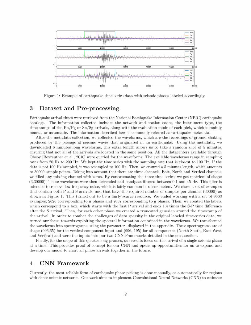
Figure 1: Example of earthquake time-series data with seismic phases labeled accordingly.

3 Dataset and Pre-processing

Earthquake arrival times were retrieved from the National Earthquake Information Center (NEIC) earthquakecatalogs. The information collected includes the network and station codes, the instrument type, thetimestamps of the Pn/Pg or Sn/Sg arrivals, along with the evaluation mode of each pick, which is mainlymanual or automatic. The information described here is commonly referred as earthquake metadata.

After the metadata collection, we collected the waveforms, which are the recordings of ground shakingproduced by the passage of seismic waves that originated in an earthquake. Using the metadata, wedownloaded 6 minutes long waveforms, this extra length allows us to take a random slice of 5 minutes,ensuring that not all of the arrivals are located in the same position. All the datacenters available throughObspy [Beyreuther et al., 2010] were queried for the waveforms. The available waveforms range in samplingrates from 20 Hz to 200 Hz. We kept the time series with the sampling rate that is closest to 100 Hz. If thedata is not 100 Hz sampled, it was resampled to 100 Hz. Then, we ensured a 5 minutes length, which amountsto 30000 sample points. Taking into account that there are three channels, East, North and Vertical channels,we filled any missing channel with zeros. By concatenating the three time series, we got matrices of shape(3,30000). These waveforms were then detrended and bandpass filtered between 0.1 and 45 Hz. This filter isintended to remove low frequency noise, which is fairly common in seismometers. We chose a set of examplesthat contain both P and S arrivals, and that have the required number of samples per channel (30000) asshown in Figure 1. This turned out to be a fairly scarce resource. We ended working with a set of 9663examples, 2626 corresponding to n phases and 7037 corresponding to g phases. Then, we created the labels,which correspond to a box, which starts with the first P arrival and ends 1.4 times the S-P time differenceafter the S arrival. Then, for each other phase we created a truncated gaussian around the timestamp ofthe arrival. In order to combat the challenges of data sparsity in the original labeled time-series data, weturned our focus towards exploiting the spectral information contained in the waveforms. We transformedthe waveforms into spectrograms, using the parameters displayed in the appendix. These spectrograms are ofshape (996,65) for the vertical component input and (996, 195) for all components (North-South, East-West,and Vertical) and were the inputs into our two CNN Frameworks detailed in the next section.

Finally, for the scope of this quarter long process, our results focus on the arrival of a single seismic phaseat a time. This provides proof of concept for our CNN and opens up opportunities for us to expand anddevelop our model to chart all phase arrivals together in the future.

4 CNN Framework

Currently, the most reliable form of earthquake phase picking is done manually, or automatically for regionswith dense seismic networks. Our work aims to implement Convolutional Neural Networks (CNN) to estimate

2

earthquake arrivals and label the phase type. In order to do so, we use a training dataset comprisedof approximately 90% of the 9,000 manually labeled 5-minute long seismic events and their respectivespectrograms. To configure the CNN framework, 10% of the original, unseen 9,000 seismic events aredesignated as a testing dataset in order to get an updated accuracy scoring on unseen data.

4.1 Baseline Model

Using inspiration from Coursera CNN labs, Tensorflow Quickguide, and [Huot, 2021], our initial baselineframework was a Keras Sequential model with an input shape of (3,30000) - this represents the seismic datain 3 dimensions (north, east, and vertical), with 30000 time-series data points. The model consisted of a1-Dimensional Convolution layer with ’same’ padding and ReLU activation, followed by batch normalizationto normalize the output according to its mean and standard deviation. It then had another 1-DimensionalConvolution layer with ’same’ padding and ReLU activation, followed by a flattening layer and dense layer tooutput the data to 4 seismic phase location predictions.

The results of the baseline test were a bit sporadic due to the low volume of input data for the baselinetest (only 100 events), but overall the results still fared relatively well for a baseline run: with a trainingaccuracy of between 30-60% and an evaluation accuracy of between 15-65%.

In order to improve our results, we converted the inputs into spectrogram data and altered the CNN tofollow a Recurrent Neural Network design, as detailed in the next section.

4.2 Updated Framework: Recurrent Neural Network

Drawing inspiration from the way human analysts detect earthquakes and the Trigger Word Detection labon Coursera, we wanted to have an architecture that takes into account information from the past and thefuture when dealing with time series. Thus, we turned to recurrent neural networks (RNN).

The final model architecture (detailed in Appendix 10.3) consisted of three layers. The first was a1-Dimensional Convolution layer followed by batch normalization, ReLU activation, and a 2% dropout. Thesecond and third layers were identical and consisted of a Bi-directional Long short-term memory (LSTM)layer, followed by batch normalization, ReLU activation, and a 2% dropout. Finally, we applied a TimeDistributed Dense layer to format the output data into an array of size (996,1). We implemented this modelin two phases: one that takes the input as the spectrogram of the vertical component, and one that takesthe input as the three individual spectrogram components. We implemented the second phase after noticingthat some of the prediction examples did not contain any discernible earthquake signal, and thus were notcontributing to the model’s learning ability. This might occur because one of the channels of the seismometeris malfunctioning, but the earthquake signal is still observed in the other channels. Both phases are discussedin the next section.

Our model was compiled using an ADAM optimizer with a learning rate of 0.0005 and a decay of 0.00001.Since we formatted our labeled data to follow box-function, composed of zeros and ones, we can think of thetask as a binary classification one, per timestep. As a consequence, we used a Binary Cross-Entropy lossfunction and examined this output, as well as a general accuracy metric to evaluate our model. We recognizethat due to the nature of the labels, accuracy might not be the best metric. Take for instance the label in theright plot of Figure 5, even if the model predicted all zeros, the accuracy would be above 90 %.

5 Experiments and Results

5.1 Hyperparameter tuning

In the initial stages of implementation, we faced the problem of the cost function becoming Not a Number,but this problem was solved by tuning the learning rate. Learning rate values of 10−5 to 10−1 were tested,with the smaller values producing the better results. The size of the mini batch was also tuned, with a batchsize of 32 examples producing the faster training times. Our results are produced using 10 epochs, due to thetime requirements to train the model, but for a longer term project we would likely during more epochs.

3

5.2 Phase 1 Results: Vertical Component Input Data

Figure 2: On the left: Binary Cross-Entropy loss value plotted over 10 epochs for Phase 1 - Vertical Componentmodel. On the right: Accuracy value plotted over 10 epochs for Phase 1 - Vertical Component model.

Figure 3: Random prediction plots of Phase 1 model. Top plots show true label versus predicted, whilebottom plots show the input data.

5.3 Phase 2 Results: 3 Component Input Data

Figure 4: On the left: Binary Cross-Entropy loss value plotted over 10 epochs for Phase 2 - 3 Componentmodel. On the right: Accuracy value plotted over 10 epochs for Phase 2 - 3 Component model.

4

Figure 5: Random prediction plots of Phase 2 model. Top plots show true label versus predicted, whilebottom plots show the 3-component input data.

6 Discussion

Phase 1 of the model, with the 1-dimensional vertical seismometer spectrogram input performed relativelywell. Figure 2 displays the loss and accuracy of this model over 10 epochs. It achieved an overall trainingloss of 0.206 and training accuracy of 92.35%, with a testing loss of 0.207 and testing accuracy of 92.23%.As seen in Figure 3, in most cases, the algorithm is able to fit the seismic arrival relatively well, however,due to the nature of seismic phase arrivals, it is possible that some events have no motion in the verticaldirection and therefore it may impact the models ability to generalize. We therefore chose to further developour algorithm to learn from all 3-directional components.

Phase 2 of the model, with the 3-dimensional seismic spectrogram inputs showed great improvement.Figure 4 shows the loss and accuracy of our phase 2 model over 10 epochs, with an overall training loss of0.151 and accuracy of 94.12%, and testing loss of 0.155 and accuracy of 94.12%. As displayed in Figure 5,the model fits the Pn seismic phase arrival overall very well, with errors primarily occurring in regions withlow signal-to-noise ratios (i.e. low quality data). Overall, this model is able to take all 3-dimensional seismicinputs and accurately identify the seismic phase arrivals, and will be further developed to predict the onsetall phases simultaneously.

7 Conclusion and Future Work

This project provides a proof of concept for the use of CNN/RNN frameworks to identify seismic phasearrivals for earthquakes. We were able to predict single phase arrivals with over 90% accuracy. This techniquecould be built upon to include the prediction of the other phases simultaneously. The ability to accuratelyand quickly identify seismic phase arrivals aids in the performance of Earthquake Early Warning and locationdetection. Future work for this project includes further developing the algorithm to simultaneously predictall Pn, Pg, Sn, and Sg phases in a single model. We also hope to collect and further process more seismicdata as it becomes available in order to continuously update our model.

8 Contributions

Both teammates made great contributions to this work. Albert Leonardo Aguilar Suarez collected andpre-processed the data. Paige Given created and tested the baseline model. Both teammates updated themodel, produced results, contributed to the presentation, and contributed to this paper.

5

9 Acknowledgements

We would like to extend a special thanks to our project TA, Shubhang Desai, for his guidance throughout thiswork. We would also like to thank all of the instructors and TAs for the CS 230 course for a very interestingand insightful quarter.

References

[Bergen et al., 2019] Bergen, K. J., P. A. Johnson, M. V. De Hoop, and G. C. Beroza, 2019, Machine learningfor data-driven discovery in solid Earth geoscience: Science, 363.

[Beyreuther et al., 2010] Beyreuther, M., R. Barsch, L. Krischer, T. Megies, Y. Behr, and J. Wassermann,2010, Obspy: A python toolbox for seismology: Seismological Research Letters, 81, 530–533.

[Huot, 2021] Huot, F., 2021, Ml-framework: https://gitlab.com/fantine/ml-framework/-/tree/

master.

[Kong et al., 2019] Kong, Q., D. T. Trugman, Z. E. Ross, M. J. Bianco, B. J. Meade, and P. Gerstoft, 2019,Machine learning in seismology: Turning data into insights: Seismological Research Letters, 90, 3–14.

[Mousavi et al., 2020] Mousavi, S. M., W. L. Ellsworth, W. Zhu, L. Y. Chuang, and G. C. Beroza, 2020,Earthquake transformer—an attentive deep-learning model for simultaneous earthquake detection andphase picking: Nature Communications, 11, 1–12.

[Ross et al., 2018] Ross, Z. E., M. A. Meier, E. Hauksson, and T. H. Heaton, 2018, Generalized seismic phasedetection with deep learning: Bulletin of the Seismological Society of America, 108, 2894–2901.

[Zhu and Beroza, 2019] Zhu, W., and G. C. Beroza, 2019, PhaseNet: A deep-neural-network-based seismicarrival-time picking method: Geophysical Journal International, 216, 261–273.

6

10 Appendix

10.1 GitHub Repository Links

Final CNN/RNN Code:https://github.com/albertleonardo/Pn/blob/master/CS230 FinalProject.ipynbData Collection Example Code:https://github.com/albertleonardo/Pn/blob/master/Example%20data.ipynbBaseline Code:https://github.com/albertleonardo/Pn/blob/master/CS230 Project PhasePicking.ipynbOther development phase code:https://github.com/albertleonardo/Pn/blob/master/numbertwo.ipynb

10.2 Spectrogram parameters

length 30000nfft 128

overlap 98sampling frequency 100

Table 1: Parameters used to generate spectrograms

7

10.3 Network architecture

10.3.1 Phase 1 - Vertical Component Input

Figure 6: Model summary for the Neural Network that takes as input the spectrograms from the verticalcomponent.

8

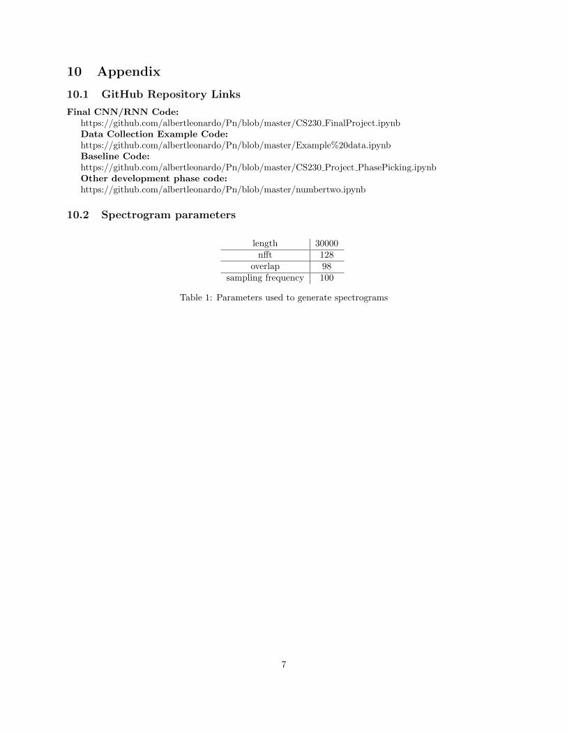
10.3.2 Phase 2 - 3 Component Input

Figure 7: Model summary for the Neural Network that takes as input the spectrograms from the threecomponents.

9