Regional Economic Conditions and the Variability of Rates of Return in Commercial Banking

Frederick Furlong and John Krainer*

Draft: September 2007

Abstract We develop new techniques to assess the relationship between commercial bank performance and the economic conditions in the markets in which they operate. In the analysis, we allow for heterogeneity in the responses of banks to regional economic conditions. We find a statistically significant relationship between bank performance and shocks to the regional markets in which they operate. We find that region-specific shocks have a significant and persistent effect on the cross-sectional variance of bank performance in the market. That is, shocks affecting average performance of banks in a region also tend to increase the dispersion of their performance. We demonstrate that this effect is due to heterogeneity in the banks’ exposures to their regional economies. Moreover, by allowing for this heterogeneity, we find that systematic responses to regional economic effects are notably more important in explaining the variation in bank performance than suggested by analysis in which responses are constrain to be the same for all banks. * Both authors are from the Federal Reserve Bank of San Francisco. We thank seminar

participants at the Federal Reserve Bank of Atlanta, Bill Keeton, and Jose Lopez for helpful discussions, and Irene Wang and Zena Knight for valuable research assistance.

The views expressed in this paper are those of the authors and not necessarily those of the Federal Reserve System.

1

Regional Economic Conditions and the Variability of Rates of Return in Commercial Banking 1. Introduction

Small banks, by virtue of their size and their emphasis on so-called relationship

banking, tend to have limited geographic scope in their activities. This is especially true

in connection with lending, with small banks tending to contract with pools of customers

from limited geographic areas. The performance of a small commercial bank, then, is

expected to be tied to the financial condition of its customers and, thus, to the economic

conditions in the local banking market.1

Contrary to this expectation, studies testing for a relationship between bank

performance and regional economic conditions find little evidence of systematic effects

of economic conditions at the county level. Yeager (2004), for example, finds that

performance of community banks in counties experiencing large economic shocks

reflected in county unemployment rates was not much different from that of similar

banks, but located in other counties. Using a different methodology, Emmons, Gilbert,

and Yeager (2004) find that rates of return at community banks in the same region were

not highly correlated in the late 1980s and early 1990s. Their results indicate that most of

the potential reduction of diversifiable risk could be achieved though local market

mergers rather than out-of-market mergers. They conclude that lack of scale, rather than

exposure to local economic conditions, accounts for an important share of community

banks’ exposure to diversifiable risk.

Studies that examine the influences of state level economic conditions find some

support for regional economic effects on bank performance. Meyer and Yeager (2001)

and Daly, Krainer, and Lopez (2007) find statistically significant effects of a variety of

measures of state economic conditions on measures of bank performance. However, in

the latter study, the model is not effective in predicting differences in problem loans for

individual banks in out-sample simulations.

1 Bank performance may also affect regional economic conditions. See Morgan, Rime, and Strahan (2002) for an analysis of how bank performance and integration affect regional economic growth.

2

A feature of most previous approaches is an assumption that the systematic

responses of bank performance measures to a change in economic conditions are the

same for all community banks. However, specialization among community banks could

lead to variation in business strategies and portfolio composition, which could, in turn,

lead to variation in the systematic responses of performance to regional economic

conditions. Also, most previous studies use measures of regional economic conditions

such as employment growth or the unemployment rate. The studies in effect assume that

the response of bank performance of a given change in the regional metric will be similar

over time and across markets. However, it seems likely the responses of performance of

banks to economic shocks driving a regional a metric could depend on the exact nature of

the shock. If so, a systematic relationship between the performance of community banks

and a measure of regional economic shocks may be difficult to detect.

In this study we present new empirical evidence based on analysis allowing for

different systematic responses by individual banks to regional economic conditions. In

the analysis, the region is the state. We also utilize measures of economic shocks related

to aggregate bank performances. While the measures still do not identify the underlying

sources of the shocks, they should reflect more reliably the relative magnitude of the

shocks with respect to banks at different points in time and across regions.

The findings suggests that accounting for differences in the systematic response

of individual banks to economic shocks is important for identifying the link between

bank performance and regional economic conditions The responses of individual banks

vary widely, ranging from significantly positive to significantly negative. The disparate

responses of community banks also means that the state shocks tend to increase the cross-

sectional variance in performance among banks in a region. This latter result is

additional evidence of regional effects on bank performance. It also is relevant to most

studies assessing the average responses to economic shocks since the increase in variance

would tend to reduce the precision of the estimated coefficients on the metrics for

regional economic conditions. The analysis reveals a complicated picture of influences

of economic conditions on community banks, one in which regional economic conditions

have been extremely important for a number of community banks, of some influence for

others, and of limited importance to the rest.

3

The paper is organized as follows. Section 2 describes the approaches used in

previous research assessing the relationship of bank performance to regional economic

conditions. Section 3 develops the framework used in this study for assessing national,

regional, and bank specific influences on rates of return for banks with identifiable

geographic markets. The data used in the empirical analysis are described in Section 4.

The empirical results regarding the effects of national and regional economic effects on

the performance of community banks are presented in Section 5. Conclusions are

presented in section 6.

2. Previous approaches to assessing regional economic influences

A common approach in the literature is to identify factors that proxy for overall

economic conditions and correlate these factors with bank performance. In this tradition,

researchers have used variables such as employment growth, unemployment rates,

income growth, home price appreciation, and indexes based on several variables as

measures of regional economic conditions. The scope of the market, or the region, is

variously defined as the state, the metropolitan area, or the county. Most studies deal

with smaller banks with regionally concentrated activities, as one is relatively confident

about defining the market correctly for this set of institutions. One exception is Daly et al.

(2007) which uses the geographic distribution of bank deposits to apportion regional

economic influences for larger, interstate banking organizations. Measures of bank

performance include rates of return on assets and equity, nonperforming assets, and

charge offs. Some studies also include bank specific variables that are expected to

influence bank performance such as loan composition.

With these variables in hand, the basic approach in most previous studies is to

assess the effects of regional influences by regressing bank performance on one or more

measures of regional economic conditions. It is common to include the lagged

performance variable in the regressions. Most of these studies seek to measure the

average effect of economic conditions on performance in a given region. An important

assumption underlying this basic approach is that effects of the underlying economic

factors, such as employment growth or real estate conditions, are similar for banks over

4

time and across regions. Another important assumption is that banks in the same region

are similar enough in their exposure to shocks that performance among banks will be

positively correlated.

Using this approach, studies focusing on narrower geographic regions such as

counties tend to find little correlation between measures of economic conditions bank

performance (Meyer and Yeager (2001) and Yeager 2003). The findings suggest that

variations in very local economic conditions are not an important source of risk for

community banks. When state level data are used, studies find some evidence of

systematic effects of economic conditions on banks (Nealy and Wheelock (1997), Meyer

and Yeager (2001), and Daly et al. (2007).

Using a much different framework, Emmons et al. (2004) also argue regional or

local market risk is not a major source of risk for community banks. Their study does not

rely on measures of regional economic conditions such as unemployment. Rather the

effects of regional conditions (local market risk) are assessed looking directly at the

correlation structure of bank return on assets in a given market. The authors simulate

hypothetical mergers to assess the potential effects on the reduction in risk among

community banks, where risk reduction is derived from reducing variance of rates of

return. The study finds that most of the risk reduction comes from in-market mergers,

rather than out of market mergers.

Emmons et al. (2004) conclude that, for community banks, most of the potential

diversification of risk could be achieved through increasing scale, rather than geographic

diversification. The implication appears to be that exposure to local economic conditions

is not a source of exposure to non-systematic (diversifiable) risk for community banks.

However, in the assessing the effects of mergers on diversification, the study does not

account for differences in business strategies (portfolio composition) among community

banks in a region. Furlong (2004) shows that bank portfolio composition can vary

considerably among community banks. Reductions in non-systematic risk in

hypothetical random mergers of community banks in a region may be due more to

increased portfolio diversification than to increased scale.

The previous studies provide valuable insights into relation of regional economic

condition and average bank performance. For example, previous research suggests that,

5

from a bank supervisory perspective, information about regional economic conditions

may not provide useful forecasts of the likely performance of an individual bank.

However, with a focus on the common or average effect of economic conditions on bank

performance, the studies may understate the degree to which regional economic

conditions affect the variability of the performance of individual banks because those

banks have different systematic responses to region-wide shocks. Indeed, competition

between banks may encourage them to specialize and find product niches (see Cohen and

Mazzeo (2004)). This strategy would tend to loosen the correlation of performance

across banks in a market in response to a particular kind of shock. To extent that this is

the case, evidence on the common or average effects of regional economic conditions

may not be a reliable guide to assessing the risk associated with limited geographic scope

for the purposes of a assessing, say, appropriate, levels of regulatory capital.

III. An alternative approach to modeling rates of return for banks

The approach we take in assessing regional economic effects is to examine their

impact on the variability of bank performance when allowing for the responses of

individual banks to economic conditions, both nationally and regionally, to vary. We

focus on rates of return (returns on assets and equity) as the measures bank performance.

Under this approach we capture the effects of national and regional factors affecting the

average bank performance by using measures of aggregate national and regional rates of

return. The impact of regional shocks is assessed in two ways. The first is the degree to

which individual bank performance is affected by the region-specific influences over

time. Second, we measure the impact of regional shocks on the distribution of bank

performance in the relevant region.

To develop the approach used in this paper, we start by noting that the

performance of the average bank located in state j can be apportioned between systematic

(aggregate) banking sector risk and idiosyncratic state-specific risk.

(1) .jt j Bt jtR Rγ ε= +

6

The systematic portion of performance, j BtRγ , owes itself to the fact that all banks are in

the same basic business, and therefore share exposure to the same basic set of shocks to

variables like interest rates and aggregate economic growth. This exposure is governed

by jγ . The term jtε represents the idiosyncratic component of state j’s banking

performance The degree of idiosyncratic risk observed in the returns of banks in a

specific state can be thought of as arising from the fact that not all state economies have

the same industry mix, demographics, and contemporaneous rates of economic growth.

A large, diversified state economy such as California may behave very similarly to the

national economy as a whole. For smaller, less-diversified economies such as Alaska,

state economic growth may look very different from the aggregate, and these differences

would likely appear in the state-specific component of Alaska’s banking sector

performance.

Using the same logic as above, we model the performance of an individual bank i

operating in state j as

(2) .ijt i jt itR Rθ η= +

The sensitivity to aggregate and state-specific factors affects individual bank i’s

performance through jtR and through its exposure to those risks, iθ . As before, the

idiosyncratic term, itη , reflects the fact that individual banks are likely to have firm-

specific components in their performance measures due to their unique circumstances,

business strategy, and customers.

Combining (1) and (2) yields,

(3) .ijt i Bt i jt itR Rβ θ ε η= + +

Equation (3) is a starting point for empirical analysis. The coefficient iβ represents the

sensitivity of an individual bank’s rate of return to the aggregate, national rate of return

(for community banks). Note that the sensitivity of bank i to aggregate shocks is given

7

by, i i jβ θ γ= . In other words, individual bank sensitivities reflect the average sensitivity

to aggregate factors in that state, scaled by that bank’s sensitivity to state factors. The

term jtε represents the regional conditions and their effect on banks, and iθ measures the

sensitivity of individual bank performance to regional conditions. The coefficients iθ

vary by bank, reflecting the potential for banks to differ according to their sensitivities to

shocks of different kinds. Community banks tend to have business strategies directed at

serving particular types of customers and providing certain types of services. Indeed, the

limited size of a community bank may dictate a choice of specialization over

diversification. As a result, in a given region, concentrations of consumer loans, business

loans, and real estate loans can vary considerably among community banks. Note that by

allowing for differences in responses to the national and regional conditions, some of

what might be considered bank-specific effects related to say, portfolio differences, are

accounted for through the coefficients iβ and iθ in equation (3). Finally, the term itη can

be thought of as capturing the effects of other bank-specific factors. For example, banks

will be exposed to the shocks that affect their individual customers, and these shocks may

not be directly related to the national or the local economy. With limited scale, small

banks will not be able to diversify away these risks, even though in expectation their

effect is zero. Also, differences in management quality would affect individual bank

performance given economic conditions and portfolio mix.

IV. The data

The empirical analysis is based on a panel data set of small commercial banks.

The data used in the empirical analysis are from the Reports of Condition (Call Reports)

filed by all domestically chartered banks in the U.S. Because we are interested in

assigning banks to a geographic region, we restrict our attention to small banks with

assets less than $1 billion.

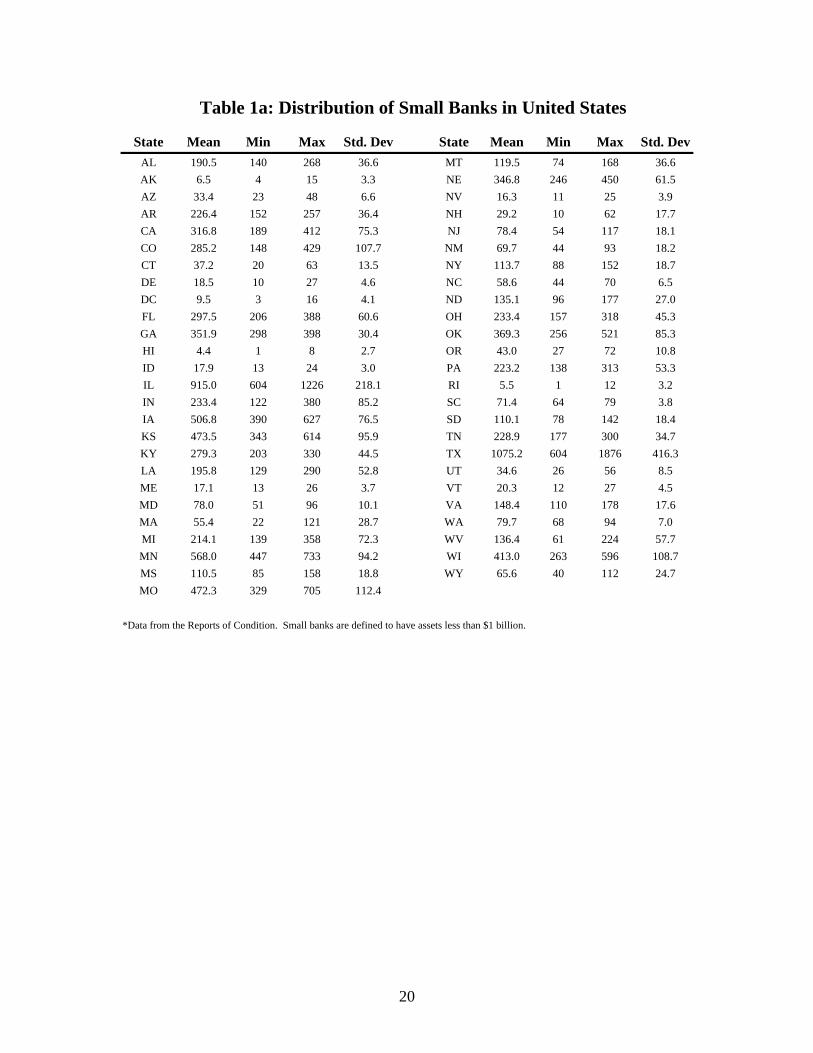
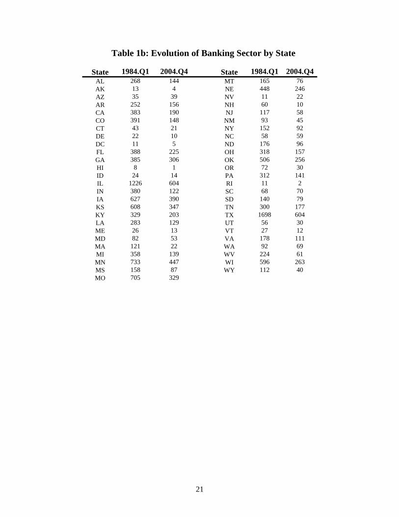
In tables 1a and 1b we report the number of small banks with usable Call Report

data in our sample period. Not surprisingly, large states tend to have more small banks,

on average. But also evident in table 1a is the legacy of the unit banking states such as

8

Illinois and Texas, which tend to have far more small banks than similarly sized states

(e.g., California). In the first quarter of 1984 there were 13,849 small banks (table 1b).

By the fourth quarter of 2004 this number fell by 50 percent to 6,954. While most states

experienced significant declines in the number of banks (the average decline over this

period was 45%), the Northeast experienced the biggest relative declines. Massachusetts

lost 82% of its small banks during this 20-year period. New Hampshire lost 83% of its

small banks. The western states experienced less decline (or consolidation) in banking

than average. Nevada experienced a doubling of the number of small banks

headquartered there over this time period.

The aggregate U.S. bank rates of return are based on the performance of all

community banks (assets less $1 billion) with useable Call Report data in a quarter. The

U.S. small bank performance over the sample period mirrors the same patterns observed

in the industry as a whole. Average return on assets (ROA) and return on equity (ROE)

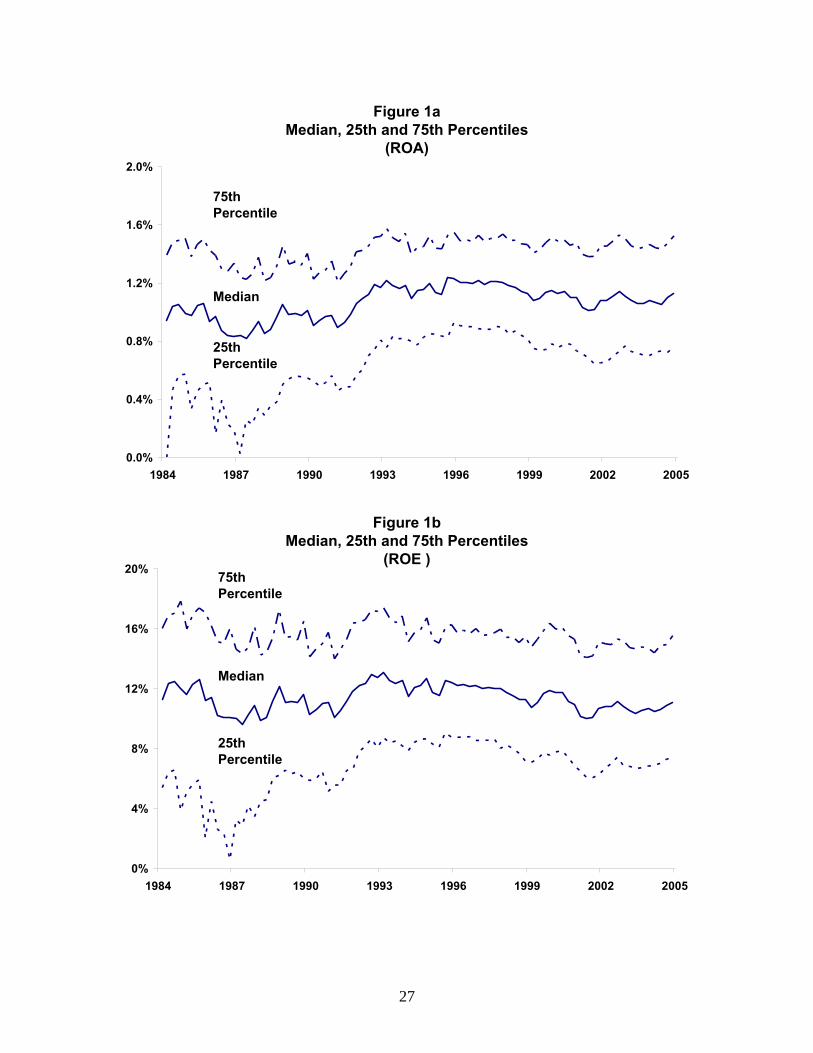
over the 25-year period were 0.8% and 9%, respectively. In figures 1a and 1b we see a

fair amount of volatility in the aggregate (small bank) performance measures. Both

measures recount the recent history in the banking sector, where bank financial condition

suffered in the late 1980s during the banking crisis, but then recovered and has remained

strong ever since. Note that the time-series of ROA and ROE associated with banks in

the 25th percentile are more volatile than the series for better-performing banks in the

distribution. Evidently, a smooth series such as aggregate ROA masks a fair degree of

heterogeneity in the cross-sectional distribution.

The aggregate regional data for bank rates of return are measured at the state level

and, again, represent the weighted-average rates of returns for all small banks with

useable Call Report data in the corresponding state in a given quarter. We focus on state

level for this study because previous studies find some support for state economic effects

on bank performance. By using states for the relevant regions, we can illustrate that even

those findings of some systematic effects of regional economic tend to understate the

impact of regional conditions on the variability of bank earnings.

9

V. Empirical finding regarding commercial bank exposures to national and regional shocks

The first stage of the empirical analysis examines the sensitivities of regional

performance to national factors. This exercise yields the state shocks which are then fed

into the individual bank regressions of performance on both national and region-specific

factors. Estimates of the relationships between state-level performances and aggregate

performance are based on the full sample (described in the previous section). The

individual bank regressions (equation (3) and its variants) are based on a balanced panel

subset of the larger data set. The balanced panel contains observations on 5,255 different

entities with continuous histories over the sample period. In these regressions we

required each state to have at least 10 observations. The measures of bank performance

are quarterly rates of return on assets (ROA) and rates of return on book-value equity

(ROE). The data series for the aggregate rates of return and for individual banking

organizations used for the balanced panel are seasonally adjusted.

Estimates of region-specific conditions

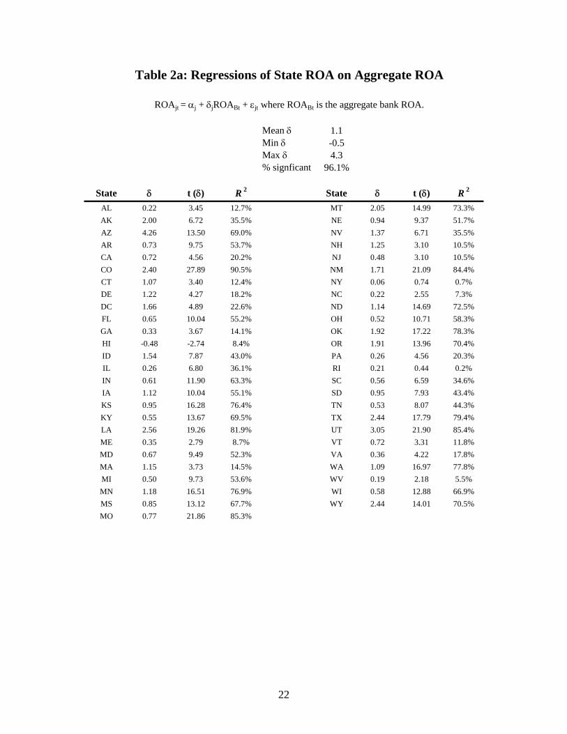
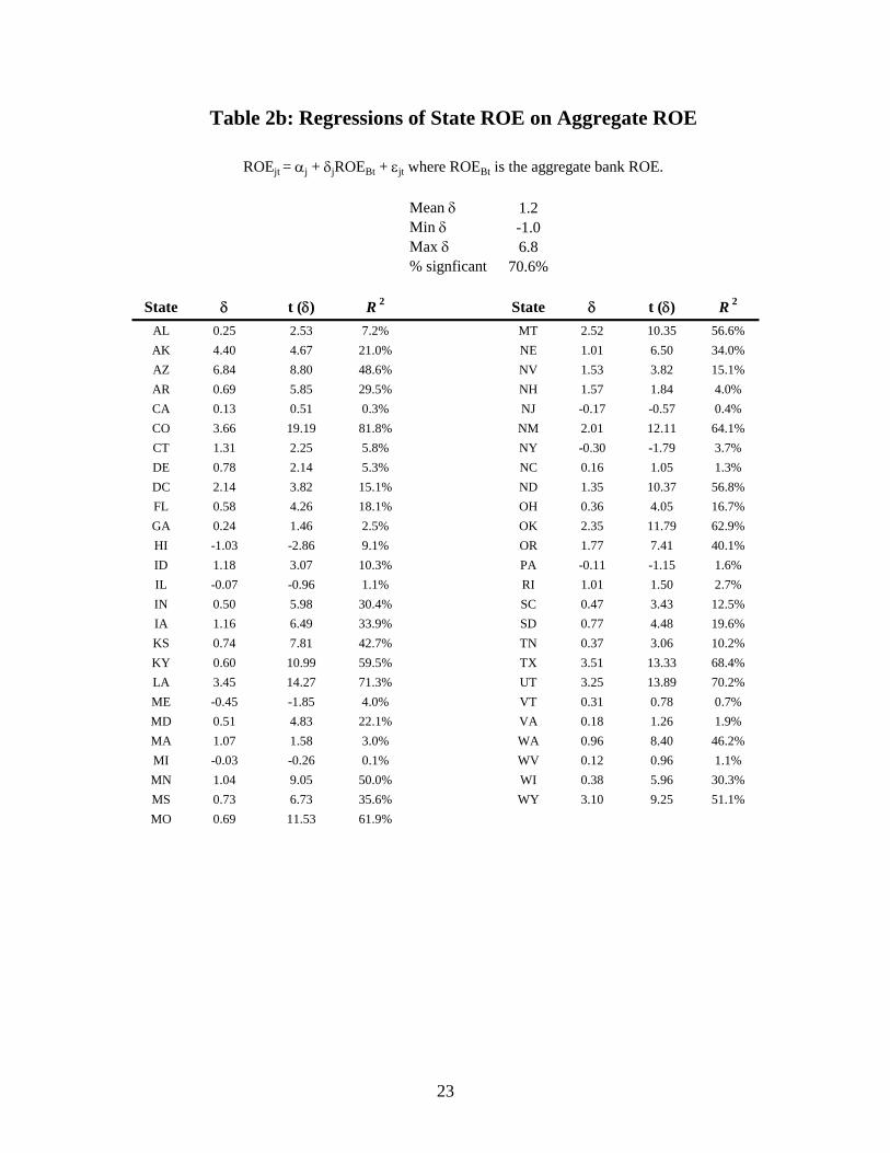
To derive the quarterly observation for the portion of the state level rates of return

associated regional conditions, we estimate equation 3 (with a constant term) separately

for each state. The results from state-by-state regressions are reported in tables 2a and

2b. The number of observations in each quarter varies among the states and over time.

The time-series variation reflects both cyclical factors (entry and exit) as well as a

declining trend in the number of banks due to consolidation.

The mean sensitivity of state ROA to aggregate (U.S.) ROA is 1.1 (1.2 for the

case of ROE in table 2b).2 About four-fifths of the coefficients on aggregate ROA and

ROE are significantly different from zero. Most, although not all, of the estimates are

positive. Still there is a fair degree of dispersion in the estimates of state sensitivity to

aggregate U.S. banking performance. For ROA, the 25th percentile and the 75th percentile

of the distribution of estimates are 0.43 and 1.45, respectively. For ROE, the 25th

2 This average value for γ across states contrasts with the weighted average γ (by assets), which must sum to one by construction.

10

percentile and the 75th percentile of the distribution of estimates are 0.27 and 1.29,

respectively. In general, the fit for the ROA regressions is better. The adjusted-R2s for

the ROA regressions range from less than 1 percent (e.g., Rhode Island) to 90 percent

(Colorado), with a median of about 50 percent, while the figures for the ROE regressions

are less than 1 percent (Michigan) to 80 percent (Colorado), with a median of 18 percent.

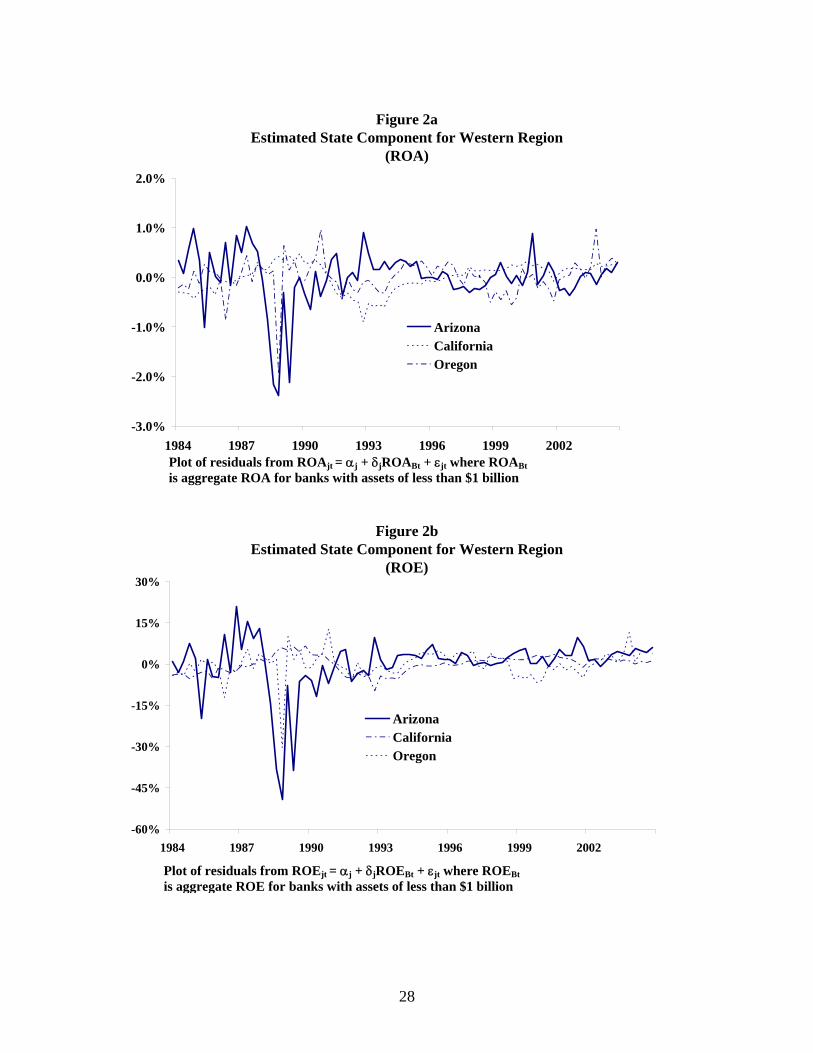
The region-specific conditions (effects) for the states are the residuals from each

of the regressions reported in tables 2a and 2b. Examples of the time series for the

region-specific components of ROA and ROE are shown in figures 2a and 2b for three

states—California, Oregon, and Arizona. The figures indicate that even for states in

relatively close proximity, regional effects can differ substantially at any point in time.

The pair-wise correlations for the state-specific components εjt in these three states never

exceed 0.2.3

The state-specific conditions for these and other states tend to be serially

correlated. This is not too surprising given the findings in previous studies that indicate

significant serial correlation in the performance of individual banks. Studies such as

Meyer and Yeager (2001) and Daly et al. (2007) find lagged performance measures are

highly significant in regression of bank performance on regional conditions.4 The

presence of serial correlation in the estimated εj’s does raise the question of how reliable

our standard errors are for the relevant coefficients.

Individual bank exposure to regional condition

The impact of economic conditions on the performance of community banks is

assessed using the framework from equation (3) for each of the panel banks. Note that

the estimation allows for variation in the responses of individual community banks to

national influences and to region-specific effects. The analysis in this section is based on

3 These low correlations at the state level point to the potential for diversification through inter-state banking. 4 Previous studies generally have not used the estimates of the lagged adjustment to assess the long-run effects of regional conditions.

11

a balanced panel of banks. We also only include the states for which the number of

observations available to estimate the state shocks was 10 or more in every quarter.5

As noted above, the state-specific shocks are serially correlated. A possible

approach, then, would be to address the serial correlation of the state-specific effects in

estimating equation (1). Since our main interest is in the second-stage regressions and

the coefficients on the state shocks and the remaining residual term, it may be

inappropriate to purge the state shocks of serial correlation. It is entirely plausible that

region-specific shocks have persistent effects on the banking sector.6 We would,

however, like the residuals in the second stage regression to be white noise. Thus, we

modify equation (3) as follows,

(4) 1, 2, 1 3, 2 4, , 3 .ijt i Bt i jt i jt i jt i j t itR Rβ θ ε θ ε θ ε θ ε η− − −= + + + + +

The results from the estimation of equation (4) (with a constant term) relating to

the distribution of the values of iβ (the sensitivity to national condition) are shown in

solid lines in figures 3a and 3b. As with the responses to the state levels of rates of return,

the coefficients for community banks vary considerably. Overall, the coefficients tend to

be positive; with about 70 percent of the sum of coefficients being positive for the ROA

equations. The 25th percentile and the 75th percentile of the distribution of estimates are

-0.2 and 1.3, respectively, with a median value of about 0.6 for the ROA equations (mean

value of about .8). For ROE, the median and mean values for the coefficient on the

national factor are about 0.6 and 1.1, respectively.7 A statistical test strongly supports the

hypotheses that the means of the coefficients for U.S. ROA and ROE are not equal to

zero.

The key parameters of interest in the model are the iθ , which measure the

sensitivity of bank i’s performance to economic conditions specific to the state. We

5 This criterion eliminated Alaska, the District of Columbia, Hawaii, and Rhode Island. 6 Berger et. al. (2000) document the persistence of bank performance. 7 Yeager (2003) points out that that convergence of regional economies over time could affect the importance of regional effects on bank performance. At the state level, economies have tended to become more diversified.

12

report statistics from the distribution of the sums of iθ in dashed lines in figures 3a and

3b. From the figures, the median values of the sums of iθ for the ROE and ROA

regressions are approximately 0.5 (the mean values are about 0.6 and 0.7, respectively).

The statistical tests strongly support the hypotheses that the means of the coefficients for

the state components of ROA and ROE are not equal to zero. Moreover, while we can

not reject the hypotheses that the estimates are from a distributions with means greater

than zero, the coefficient on the state components of ROA and ROE are negative and

statistically significant for a minority of banks in the panel. Among the results from the

individual bank regressions for ROA, about 40% of the sums of the coefficients on the

state shocks are positive and significantly different from zero and another 10% are

negative and statistically significant. The results for the ROE regressions are 42%

positive and 12% negative and significant.

The results from statistical analysis also highlight the considerable variation in

the systematic responses of the performance of individual banks to factors affecting

banks nationally and in their respective states. The variation in the response to state-

specific conditions also is somewhat larger than that for the responses to national

conditions. For example, the inter-quartile range for the distribution of iβ is 1.26 for

ROA, compared to 1.5 for the sum of iθ coefficients. It is also worth noting that the

variation in the sums of iθ is present not only among banks in different states, but also

among banks in the same state.

The interpretation of the results is that state shocks can have a potentially large

effect on individual bank performance. The size of this effect depends not only on the

size of the shock, but also on the varying degree to which banks are positioned to be

affected by the shock. Banks with large θ’s have apparently selected strategies that, at

least ex-post, made them more vulnerable to shocks typical in their regional (in this case

state) markets. The wide variation in even the systematic responses of community banks

to state shocks may be part of the reason that previous research has found regional

economic conditions do little to improve out-of-sample forecasts of bank performance.

Moreover, it also is possible that the range of systematic responses, significantly negative

to significantly positive, found using state level data may also be indicative of community

13

bank exposures at narrower geographic aggregations, such as counties and may mask the

role of regional shocks when assessed by the average impact.

Regional shocks and the cross-sectional distribution of community bank performance

The variation in systematic response to state-specific (as well as national)

economic conditions (i.e., shocks to those conditions) suggests that the effect of state-

specific conditions should be assessed not just on the average effect on community bank

performance, but also on the distribution of bank performance. The next steps in the

empirical analysis are to assess the effect of state shocks on the variance of return for the

individual community banks and the effects of state shocks to the distribution of rates of

return in a given state

In examining the effects on the cross-sectional distributions of rates of returns

among banks in the same state, we include ROA and ROE for all community banks with

useable Call Reports in a given state and quarter. The approach is to examine how the

value of a regional shock at a point in time affects the distribution of bank performance.

The idea is that, if banks are affected differentially by regional shocks, then regional

shocks should increase the dispersion of performance.

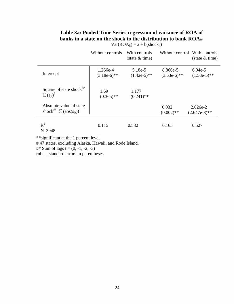
For this analysis, then, we compute the variance of the distribution of ROA and

ROE for each state for each quarter over the sample period. The magnitude of regional

shocks is measured in two ways—the absolute value of shock, jtε , and the square of the

shocks, ( )2

jtε . The observations then are quarterly for each state. For each state, we first

use pooled-cross sectional regressions where the dependent variable is variance of the

rates of return (ROA or ROE) of all banks in a state at time t and the explanatory variable

is either the absolute value of the regional shock (or the square of the shock) at time t.

We use pooled cross-section regressions for all the states with state-fixed effects.

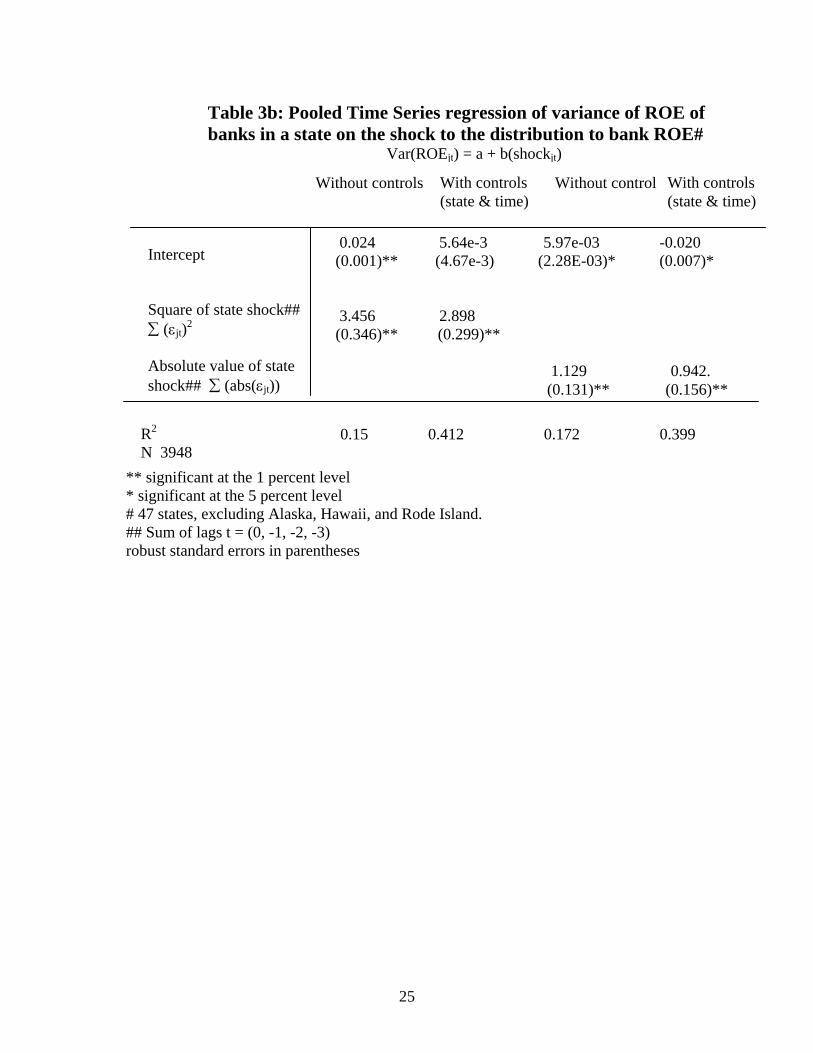
The results for the regressions are shown in tables 3a and 3b. In the pooled cross-

section the measures of the dispersion of bank performances are positively and

significantly related to both metrics of the state-level shocks. As indicated, the

regressions were estimated with and without controlling for state-specific and time period

14

(quarterly) effects.8 The main result in this section is that the effects of the shocks on the

variances of performance are positively correlated with variation in the sums of the

coefficients iθ . This indicates that the effects of regional shock to banking are manifested

in the distribution of bank performance within a state. To the extent that regional shocks

tend to increase the variance of performance of banks in a region, this would tend to

make it more difficult to reject the hypothesis that regional shocks do not affect bank

performance when the test is on the effects on the level of ROA or ROE of banks.

Evidently, regional economic conditions have a statistically significant effect on the

variance of bank performance in a given market, even while the effect of economic

conditions on average performance might be muted.

We continue the analysis by exploring the dynamic relationship between regional

shocks and the distribution of bank performance. Towards this end, the basic relationship

between shocks to a banking market and their effect on the distribution of performance in

that market can be summarized using a vector autoregression (VAR). In this exercise we

estimate a pooled VAR,

(6) 0 1 1 2 2 3 3 4 4 ,jt jt jt jt jt jtY Y Y Y Yφ φ φ φ φ ν− − − −= + + + + +

where Yjt is a two-dimensional vector containing the variance of ROA (or ROE) in a

given state j at time t and a measure of the state shock at time t: alternatively, jtε or

( )2

jtε for each state j. The 2x1 vector υt is a white noise process uncorrelated with Yt.

The pooling refers to pooling across states, so that the coefficients in equation (6) should

be interpreted as average effects. To avoid problems associated with survivorship bias,

the results presented below are based on the full sample (i.e., not the balanced panel).9

8 Binary (zero-one) dummies variables were included to control for time invariant factors for the states and state invariant factors for each quarter. In the tables, the robust standard errors are reported in parenthesis. 9 We conducted the same exercise for the balanced panel and found the same qualitative results. However, the magnitude of the relationship between the variance of state-level rates of return and the state shock was smaller, as the survivor firms in the balanced panel exhibit less volatility over the sample period.

15

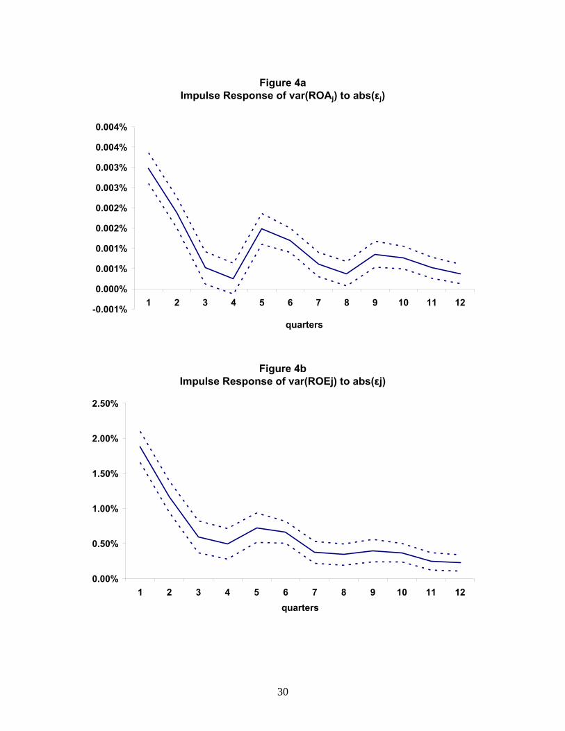
Figures 4a and 4b plot a two standard deviation shock to jtε for both ROA and

ROE. In 4a, note that even a two standard deviation shock is quite small. This reflects

the fact that ROA in general is both small and not that variable in the banking data. The

figure shows, however, that the average effect of changes in the state shock has a

significant effect on the cross sectional variance of ROA in the state. The effect is

significant immediately at the one quarter lag, and is persistent and positive out to 12

quarters. The same basic patterns are even more evident in figure 4b, where we plot the

impulse response of the variance of ROE to a shock to jtε . Indeed, the magnitude of the

effect is much larger for the more volatile ROE. A one standard deviation shock to jtε

initially moves the average variance of state ROE by about 2 percentage points. To put

this into perspective, the average variance of state ROE is about 3 percent over our

sample period.

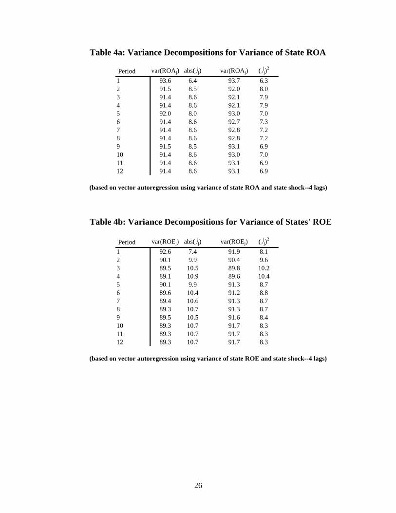
To quantify the relationships in figures 4a and 4b, we perform a variance

decomposition of the VAR in equation (6).10 The results of this decomposition are in

Tables 4a and 4b. Evidently, the state shock accounts for approximately 8 percent of the

explained variation in the state ROA variance over the 12 quarter horizon, with own

variance explaining the remainder. As before, the results are similar for ROE. The state

shock accounts for about 10 percent of the explained variation in state ROE variance

consistently over the 12 period horizon.

We also consider the effects of state shocks on the idiosyncratic variance of bank

performance in a market using the VAR framework. By replacing var(Rjt) in the vector Yt

(equation 6) with var(ηjt) from equation (5), we can re-estimate the VAR and simulate the

response of the variance of bank-specific risk in a market to a shock to economic

conditions.11 The impulse responses are much smaller, and are generally insignificantly

different from zero, after the initial period. However, the impulse responses after

controlling for regional effects suggest that the changing nature of the shocks themselves

have some impact on the distribution of bank performance in a state. To the extent that

10 We use the Cholesky decomposition in this exercise. 11 To be precise, var(ηjt) is computed by estimating ηijt for the balanced panel (equation 4), and taking the cross-sectional variance of ηit for all banks in market j. The time-series var(ηjt) for each market j is then inserted into the VAR in equation 6.

16

shocks differ in a particular market and over time, some of the variation at a particular

point in time will be embedded in our residuals from the estimation of equation (4) for

banks in the panel.

Time series variance for individual banks

The evidence so far indicates that regional shocks had statistically significant

effects on the performance of about one-half the community banks in our sample.

Moreover, the effects of state shocks are evident in the distribution of the performance of

community banks. In the next steps we consider the extent to which taking into account

differences in the sensitivity of individual banks reduces the measured variation in their

rates of return over time. In particular, we compare the distribution of the adjusted R2

statistics from the two models of rates of returns for individual banks. For the first set,

R2s were derived for each bank in the panel from regressions of ROA and ROE on

aggregate U.S. ROA and ROE. The second set of R2s is from the estimates of equation 4,

which includes both the national and state-specific component of rates of return.

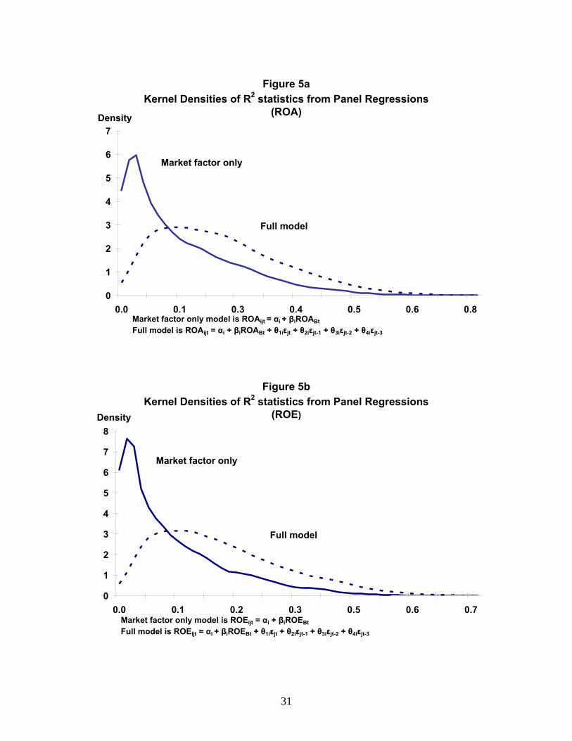
The distributions of the R2s are shown in figures 5a and 5b. For the U.S. market factor-

only model of ROA, the mean R2-adjusted statistic for the 5,255 bank-regressions is 12%.

Including the state shocks as explanatory variables raises the mean R2 to 22%. For the

ROE regressions, the comparable statistics are a mean R2s of 10% for the U.S. market-

factor only model and a mean R2s of 21% when the state shocks are included.

Kolmogorov-Smirnov tests for equality between the distributions in 5a and 5b easily

reject the null hypothesis that the pairs of distributions are equal (in each case, with p-

value 0.0). Also of note is the prominent skew to the distributions. For some banks,

adding state effects goes a long way towards accounting for the variation of its

performance over time.12

12 Moreover, the analysis only captures systematic effects. The degree of the systematic relationship can depend on the extent and type of specialization of a bank and the nature of the economic shocks. For example, a state’s shocks might hit different economic sectors—commercial real estate, aerospace, IT, subprime residential real estate loans—at different points in time. In that case, the performance of a community bank with a diversified loan portfolio might exhibit a high degree of systematic exposure to state shocks. In contrast, a highly specialized bank likely would exhibit a low degree of systematic exposure, even though the bank would be affected by economic conditions in its own sector of specialization. Those effects would be measured as idiosyncratic effects.

17

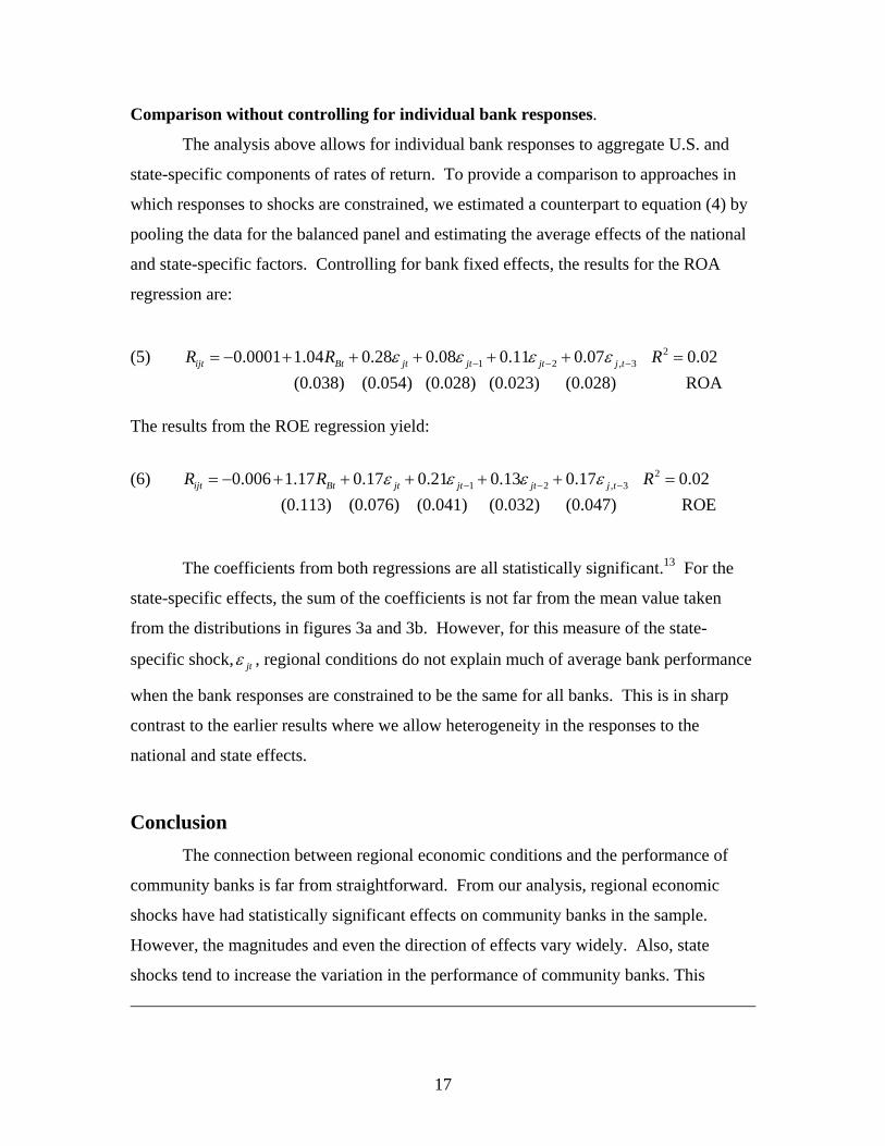
Comparison without controlling for individual bank responses.

The analysis above allows for individual bank responses to aggregate U.S. and

state-specific components of rates of return. To provide a comparison to approaches in

which responses to shocks are constrained, we estimated a counterpart to equation (4) by

pooling the data for the balanced panel and estimating the average effects of the national

and state-specific factors. Controlling for bank fixed effects, the results for the ROA

regression are:

(5) 21 2 , 30.0001 1.04 0.28 0.08 0.11 0.07 0.02ijt Bt jt jt jt j tR R Rε ε ε ε− − −= − + + + + + =

(0.038) (0.054) (0.028) (0.023) (0.028) ROA The results from the ROE regression yield:

(6) 21 2 , 30.006 1.17 0.17 0.21 0.13 0.17 0.02ijt Bt jt jt jt j tR R Rε ε ε ε− − −= − + + + + + =

(0.113) (0.076) (0.041) (0.032) (0.047) ROE

The coefficients from both regressions are all statistically significant.13 For the

state-specific effects, the sum of the coefficients is not far from the mean value taken

from the distributions in figures 3a and 3b. However, for this measure of the state-

specific shock, jtε , regional conditions do not explain much of average bank performance

when the bank responses are constrained to be the same for all banks. This is in sharp

contrast to the earlier results where we allow heterogeneity in the responses to the

national and state effects.

Conclusion The connection between regional economic conditions and the performance of

community banks is far from straightforward. From our analysis, regional economic

shocks have had statistically significant effects on community banks in the sample.

However, the magnitudes and even the direction of effects vary widely. Also, state

shocks tend to increase the variation in the performance of community banks. This

18

finding is additional evidence of regional effects on bank performance. It also is relevant

to most studies assessing the average responses to economic shocks since the increase in

variance would tend to reduce the precision of the estimated coefficients. This is

illustrated by the comparison of the results from the bank-by-bank analysis, which allow

for heterogeneous responses to state-specific shocks, and the pooled cross-section time

series analysis, in which responses of individual banks’ rates of return to the state effects

are constrain to be the same for all banks.

These results suggest that community banks are exposed to greater regional risk

than suggested by previous studies. At the same time, the analysis points to the difficulty

of drawing inferences about the implications of regional economic shocks for individual

community banks. There is the wide range of systematic responses of community. The

systematic responses reflect the interaction of individual bank strategies and the makeup

of the combination of shocks in a given state over the sample period. In addition, the

performance of most community banks still appears to be related in large part to bank-

specific factors. This suggests that, even accounting for a bank’s specific exposure to

systematic risk (national and regional effects), its risk management and general business

practices, as well as its customer base, likely will be very important in accounting for the

variability of its performance over time.

13 Robust standard errors are reported in parentheses.

19

References

Acharya, V., Hasan, I., and Saunders, A., 2002. “Should Banks Be Diversified? Evidence from Individual Bank Loan Portfolios.” BIS working paper. Berger, A., Bonime, S., Covitz, D., and Hancock, D., 2000. “Why are Bank Profits so Persistent? The Roles of Product Market Competition, Informational Opacity, and Regional/Macroeconomic Shocks.” Journal of Banking and Finance, vol. 24 (July 2000), pp. 1203-35. Cohen, A., and Mazzeo, M., 2004. “Market Structure and Competition Amongst Retail Depository Institutions.” Federal Reserve Board of Governors working paper. Daly, M. C., Krainer, J., and Lopez, J., (2003), “Regional Economic Conditions and Aggregate Bank Performance.” Forthcoming in Research in Finance. Emmons, W., Gilbert A., and Yeager T., (2004). “Risk Reduction at Small Community Banks: Is it Size of Geographic Diversification that Matters?” Journal of Financial Services Research 25 2/3, pp. Furlong F. T., (2004). “Comment on Emmons, Gilbert, and Yeager” Journal of Financial Services Research 25 2/3, pp. 283-289. Krainer, J., 2001. “Banking and the Business Cycle.” Federal Reserve Bank of San Francisco Economic Letter. Meyers, A. P., and Yeager, T. J., (2001), “Are Small Rural Banks Vulnerable to Local Economic Downturns?” Federal Reserve Bank of St. Louis Review, 83, pp. 25-38. Morgan, D., Rime, B., and Strahan, P., 2002. “Bank Integration and State Business Cycles.” Working paper. Morgan, D., and Samolyk, K., 2003. “Geographic Diversification and Bank Performance.” Working paper. Neely, M. and Wheelock, D. (1997) “Why Does Bank Performance Vary Across States?” Federal Reserve Bank of St. Louis Review 79, pp 27-40. Yeager, T. J., (2004), “The Demise of Community Banks? Local Economic Shocks are not to Blame.” Journal of Banking and Finance 28, pp 2135-2153.

20

Table 1a: Distribution of Small Banks in United States

State Mean Min Max Std. Dev State Mean Min Max Std. DevAL 190.5 140 268 36.6 MT 119.5 74 168 36.6AK 6.5 4 15 3.3 NE 346.8 246 450 61.5AZ 33.4 23 48 6.6 NV 16.3 11 25 3.9AR 226.4 152 257 36.4 NH 29.2 10 62 17.7CA 316.8 189 412 75.3 NJ 78.4 54 117 18.1CO 285.2 148 429 107.7 NM 69.7 44 93 18.2CT 37.2 20 63 13.5 NY 113.7 88 152 18.7DE 18.5 10 27 4.6 NC 58.6 44 70 6.5DC 9.5 3 16 4.1 ND 135.1 96 177 27.0FL 297.5 206 388 60.6 OH 233.4 157 318 45.3GA 351.9 298 398 30.4 OK 369.3 256 521 85.3HI 4.4 1 8 2.7 OR 43.0 27 72 10.8ID 17.9 13 24 3.0 PA 223.2 138 313 53.3IL 915.0 604 1226 218.1 RI 5.5 1 12 3.2IN 233.4 122 380 85.2 SC 71.4 64 79 3.8IA 506.8 390 627 76.5 SD 110.1 78 142 18.4KS 473.5 343 614 95.9 TN 228.9 177 300 34.7KY 279.3 203 330 44.5 TX 1075.2 604 1876 416.3LA 195.8 129 290 52.8 UT 34.6 26 56 8.5ME 17.1 13 26 3.7 VT 20.3 12 27 4.5MD 78.0 51 96 10.1 VA 148.4 110 178 17.6MA 55.4 22 121 28.7 WA 79.7 68 94 7.0MI 214.1 139 358 72.3 WV 136.4 61 224 57.7MN 568.0 447 733 94.2 WI 413.0 263 596 108.7MS 110.5 85 158 18.8 WY 65.6 40 112 24.7MO 472.3 329 705 112.4

*Data from the Reports of Condition. Small banks are defined to have assets less than $1 billion.

21

Table 1b: Evolution of Banking Sector by State

State 1984.Q1 2004.Q4 State 1984.Q1 2004.Q4AL 268 144 MT 165 76AK 13 4 NE 448 246AZ 35 39 NV 11 22AR 252 156 NH 60 10CA 383 190 NJ 117 58CO 391 148 NM 93 45CT 43 21 NY 152 92DE 22 10 NC 58 59DC 11 5 ND 176 96FL 388 225 OH 318 157GA 385 306 OK 506 256HI 8 1 OR 72 30ID 24 14 PA 312 141IL 1226 604 RI 11 2IN 380 122 SC 68 70IA 627 390 SD 140 79KS 608 347 TN 300 177KY 329 203 TX 1698 604LA 283 129 UT 56 30ME 26 13 VT 27 12MD 82 53 VA 178 111MA 121 22 WA 92 69MI 358 139 WV 224 61MN 733 447 WI 596 263MS 158 87 WY 112 40MO 705 329

22

Table 2a: Regressions of State ROA on Aggregate ROA

ROAjt = αj + δjROABt + εjt where ROABt is the aggregate bank ROA.

Mean δ 1.1Min δ -0.5Max δ 4.3% signficant 96.1%

State δ t (δ) R 2 State δ t (δ) R 2

AL 0.22 3.45 12.7% MT 2.05 14.99 73.3%AK 2.00 6.72 35.5% NE 0.94 9.37 51.7%AZ 4.26 13.50 69.0% NV 1.37 6.71 35.5%AR 0.73 9.75 53.7% NH 1.25 3.10 10.5%CA 0.72 4.56 20.2% NJ 0.48 3.10 10.5%CO 2.40 27.89 90.5% NM 1.71 21.09 84.4%CT 1.07 3.40 12.4% NY 0.06 0.74 0.7%DE 1.22 4.27 18.2% NC 0.22 2.55 7.3%DC 1.66 4.89 22.6% ND 1.14 14.69 72.5%FL 0.65 10.04 55.2% OH 0.52 10.71 58.3%GA 0.33 3.67 14.1% OK 1.92 17.22 78.3%HI -0.48 -2.74 8.4% OR 1.91 13.96 70.4%ID 1.54 7.87 43.0% PA 0.26 4.56 20.3%IL 0.26 6.80 36.1% RI 0.21 0.44 0.2%IN 0.61 11.90 63.3% SC 0.56 6.59 34.6%IA 1.12 10.04 55.1% SD 0.95 7.93 43.4%KS 0.95 16.28 76.4% TN 0.53 8.07 44.3%KY 0.55 13.67 69.5% TX 2.44 17.79 79.4%LA 2.56 19.26 81.9% UT 3.05 21.90 85.4%ME 0.35 2.79 8.7% VT 0.72 3.31 11.8%MD 0.67 9.49 52.3% VA 0.36 4.22 17.8%MA 1.15 3.73 14.5% WA 1.09 16.97 77.8%MI 0.50 9.73 53.6% WV 0.19 2.18 5.5%MN 1.18 16.51 76.9% WI 0.58 12.88 66.9%MS 0.85 13.12 67.7% WY 2.44 14.01 70.5%MO 0.77 21.86 85.3%

23

Table 2b: Regressions of State ROE on Aggregate ROE

ROEjt = αj + δjROEBt + εjt where ROEBt is the aggregate bank ROE.

Mean δ 1.2Min δ -1.0Max δ 6.8% signficant 70.6%

State δ t (δ) R 2 State δ t (δ) R 2

AL 0.25 2.53 7.2% MT 2.52 10.35 56.6%AK 4.40 4.67 21.0% NE 1.01 6.50 34.0%AZ 6.84 8.80 48.6% NV 1.53 3.82 15.1%AR 0.69 5.85 29.5% NH 1.57 1.84 4.0%CA 0.13 0.51 0.3% NJ -0.17 -0.57 0.4%CO 3.66 19.19 81.8% NM 2.01 12.11 64.1%CT 1.31 2.25 5.8% NY -0.30 -1.79 3.7%DE 0.78 2.14 5.3% NC 0.16 1.05 1.3%DC 2.14 3.82 15.1% ND 1.35 10.37 56.8%FL 0.58 4.26 18.1% OH 0.36 4.05 16.7%GA 0.24 1.46 2.5% OK 2.35 11.79 62.9%HI -1.03 -2.86 9.1% OR 1.77 7.41 40.1%ID 1.18 3.07 10.3% PA -0.11 -1.15 1.6%IL -0.07 -0.96 1.1% RI 1.01 1.50 2.7%IN 0.50 5.98 30.4% SC 0.47 3.43 12.5%IA 1.16 6.49 33.9% SD 0.77 4.48 19.6%KS 0.74 7.81 42.7% TN 0.37 3.06 10.2%KY 0.60 10.99 59.5% TX 3.51 13.33 68.4%LA 3.45 14.27 71.3% UT 3.25 13.89 70.2%ME -0.45 -1.85 4.0% VT 0.31 0.78 0.7%MD 0.51 4.83 22.1% VA 0.18 1.26 1.9%MA 1.07 1.58 3.0% WA 0.96 8.40 46.2%MI -0.03 -0.26 0.1% WV 0.12 0.96 1.1%MN 1.04 9.05 50.0% WI 0.38 5.96 30.3%MS 0.73 6.73 35.6% WY 3.10 9.25 51.1%MO 0.69 11.53 61.9%

24

**significant at the 1 percent level # 47 states, excluding Alaska, Hawaii, and Rode Island. ## Sum of lags t = (0, -1, -2, -3) robust standard errors in parentheses

Table 3a: Pooled Time Series regression of variance of ROA of banks in a state on the shock to the distribution to bank ROA#

Var(ROAjt) = a + b(shockjt)

Intercept Square of state shock## ∑ (εjt)2

Absolute value of state shock## ∑ (abs(εjt))

Without controls With controls (state & time)

Without controls With controls (state & time)

R2 N 3948

1.266e-4 5.18e-5 8.866e-5 6.04e-5 (3.18e-6)** (1.42e-5)** (3.53e-6)** (1.53e-5)**

1.69 1.177 (0.365)** (0.241)** 0.032 2.026e-2 (0.002)** (2.647e-3)**

0.115 0.532 0.165 0.527

25

** significant at the 1 percent level * significant at the 5 percent level # 47 states, excluding Alaska, Hawaii, and Rode Island. ## Sum of lags t = (0, -1, -2, -3) robust standard errors in parentheses

Table 3b: Pooled Time Series regression of variance of ROE of banks in a state on the shock to the distribution to bank ROE#

Var(ROEjt) = a + b(shockjt)

Intercept Square of state shock## ∑ (εjt)2

Absolute value of state shock## ∑ (abs(εjt))

Without controls With controls (state & time)

Without controls With controls (state & time)

R2

N 3948

0.024 5.64e-3 5.97e-03 -0.020 (0.001)** (4.67e-3) (2.28E-03)* (0.007)*

3.456 2.898 (0.346)** (0.299)** 1.129 0.942. (0.131)** (0.156)**

0.15 0.412 0.172 0.399

26

Table 4a: Variance Decompositions for Variance of State ROA

Period var(ROAj) abs(⎠ j) var(ROAj) (⎠j)2

1 93.6 6.4 93.7 6.32 91.5 8.5 92.0 8.03 91.4 8.6 92.1 7.94 91.4 8.6 92.1 7.95 92.0 8.0 93.0 7.06 91.4 8.6 92.7 7.37 91.4 8.6 92.8 7.28 91.4 8.6 92.8 7.29 91.5 8.5 93.1 6.910 91.4 8.6 93.0 7.011 91.4 8.6 93.1 6.912 91.4 8.6 93.1 6.9

(based on vector autoregression using variance of state ROA and state shock--4 lags)

Table 4b: Variance Decompositions for Variance of States' ROE

Period var(ROEj) abs(⎠ j) var(ROEj) (⎠j)2

1 92.6 7.4 91.9 8.12 90.1 9.9 90.4 9.63 89.5 10.5 89.8 10.24 89.1 10.9 89.6 10.45 90.1 9.9 91.3 8.76 89.6 10.4 91.2 8.87 89.4 10.6 91.3 8.78 89.3 10.7 91.3 8.79 89.5 10.5 91.6 8.410 89.3 10.7 91.7 8.311 89.3 10.7 91.7 8.312 89.3 10.7 91.7 8.3

(based on vector autoregression using variance of state ROE and state shock--4 lags)

27

Figure 1aMedian, 25th and 75th Percentiles

(ROA)

0.0%

0.4%

0.8%

1.2%

1.6%

2.0%

1984 1987 1990 1993 1996 1999 2002 2005

Median

25th Percentile

75thPercentile

Figure 1bMedian, 25th and 75th Percentiles

(ROE )

0%

4%

8%

12%

16%

20%

1984 1987 1990 1993 1996 1999 2002 2005

Median

25th Percentile

75thPercentile

28

Figure 2aEstimated State Component for Western Region

(ROA)

-3.0%

-2.0%

-1.0%

0.0%

1.0%

2.0%

1984 1987 1990 1993 1996 1999 2002

ArizonaCaliforniaOregon

Plot of residuals from ROAjt = αj + δjROABt + εjt where ROABt is aggregate ROA for banks with assets of less than $1 billion

Figure 2bEstimated State Component for Western Region

(ROE)

-60%

-45%

-30%

-15%

0%

15%

30%

1984 1987 1990 1993 1996 1999 2002

ArizonaCaliforniaOregon

Plot of residuals from ROEjt = αj + δjROEBt + εjt where ROEBt is aggregate ROE for banks with assets of less than $1 billion

29

0

0.1

0.2

0.3

0.4

0.5

-5 0 5 10 15

Responses to NationalROA

Responses to StateComponents of ROA

Figure 3a Distributions of Responses of Individual Community

Banks' ROA to National and State ComponentsDensity

Model is ROAijt = αi + βiROABt + θ1iεjt + θ2iεjt-1 + θ3iεjt-2 + θ4iεjt-3 + ηit

0

0.1

0.2

0.3

0.4

0.5

-5 0 5 10 15

Responses to NationalROE

Responses to StateComponents of ROE

Figure 3b Distributions of Responses of Individual Community Banks'

ROE to National and State ComponentsDensity

Model is ROEijt = αi + βiROEBt + θ1iεjt + θ2iεjt-1 + θ3iεjt-2 + θ4iεjt-3 + ηit

30

Figure 4aImpulse Response of var(ROAj) to abs(εj)

-0.001%

0.000%

0.001%

0.001%

0.002%

0.002%

0.003%

0.003%

0.004%

0.004%

1 2 3 4 5 6 7 8 9 10 11 12

quarters

Figure 4bImpulse Response of var(ROEj) to abs(εj)

0.00%

0.50%

1.00%

1.50%

2.00%

2.50%

1 2 3 4 5 6 7 8 9 10 11 12quarters

31

Figure 5aKernel Densities of R2 statistics from Panel Regressions

(ROA)

0

1

2

3

4

5

6

7

0.0 0.1 0.3 0.4 0.5 0.6 0.8

Density

Market factor only model is ROAijt = αi + βiROABt

Full model is ROAijt = αi + βiROABt + θ1iεjt + θ2iεjt-1 + θ3iεjt-2 + θ4iεjt-3

Market factor only

Full model

Figure 5bKernel Densities of R2 statistics from Panel Regressions

(ROE)

0

1

2

3

4

5

6

7

8

0.0 0.1 0.2 0.3 0.5 0.6 0.7

Density

Market factor only model is ROEijt = αi + βiROEBt

Full model is ROEijt = αi + βiROEBt + θ1iεjt + θ2iεjt-1 + θ3iεjt-2 + θ4iεjt-3

Market factor only

Full model