REGIONAL FORECAST OF JOBS, POPULATION …2040.planbayarea.org/sites/default/files/2017-07/Regional Forecast...Supervisor Nathan Miley Alameda Supervisor Candace Andersen Contra Costa

REGIONAL FORECAST OF JOBS, POPULATION AND HOUSING

FINAL SUPPLEMENTAL REPORT

JULY 2017

Metropolitan Transportation Commission

Association of Bay Area Governments

Metropolitan Transportation Commission

Jake Mackenzie, ChairSonoma County and Cities

Scott Haggerty, Vice ChairAlameda County

Alicia C. AguirreCities of San Mateo County

Tom AzumbradoU.S. Department of Housing and Urban Development

Jeannie BruinsCities of Santa Clara County

Damon ConnollyMarin County and Cities

Dave CorteseSanta Clara County

Carol Dutra-VernaciCities of Alameda County

Dorene M. GiacopiniU.S. Department of Transportation

Federal D. GloverContra Costa County

Anne W. HalstedSan Francisco Bay Conservation and Development Commission

Nick JosefowitzSan Francisco Mayor’s Appointee

Jane Kim City and County of San Francisco

Sam LiccardoSan Jose Mayor’s Appointee

Alfredo Pedroza Napa County and Cities

Julie PierceAssociation of Bay Area Governments

Bijan SartipiCalifornia State Transportation Agency

Libby SchaafOakland Mayor’s Appointee

Warren Slocum San Mateo County

James P. SperingSolano County and Cities

Amy R. WorthCities of Contra Costa County

Association of Bay Area Governments

Councilmember Julie Pierce ABAG PresidentCity of Clayton

Supervisor David Rabbitt ABAG Vice PresidentCounty of Sonoma

Representatives From Each CountySupervisor Scott HaggertyAlameda

Supervisor Nathan MileyAlameda

Supervisor Candace AndersenContra Costa

Supervisor Karen MitchoffContra Costa

Supervisor Dennis RodoniMarin

Supervisor Belia RamosNapa

Supervisor Norman YeeSan Francisco

Supervisor David CanepaSan Mateo

Supervisor Dave PineSan Mateo

Supervisor Cindy ChavezSanta Clara

Supervisor David CorteseSanta Clara

Supervisor Erin HanniganSolano

Representatives From Cities in Each CountyMayor Trish SpencerCity of Alameda / Alameda

Mayor Barbara HallidayCity of Hayward / Alameda

Vice Mayor Dave Hudson City of San Ramon / Contra Costa

Councilmember Pat Eklund City of Novato / Marin

Mayor Leon GarciaCity of American Canyon / Napa

Mayor Edwin LeeCity and County of San Francisco

John Rahaim, Planning DirectorCity and County of San Francisco

Todd Rufo, Director, Economic and Workforce Development, Office of the MayorCity and County of San Francisco

Mayor Wayne LeeCity of Millbrae / San Mateo

Mayor Pradeep GuptaCity of South San Francisco / San Mateo

Mayor Liz GibbonsCity of Campbell / Santa Clara

Mayor Greg ScharffCity of Palo Alto / Santa Clara

Mayor Len AugustineCity of Vacaville / Solano

Mayor Jake MackenzieCity of Rohnert Park / Sonoma

Councilmember Annie Campbell Washington City of Oakland / Alameda

Councilmember Lynette Gibson McElhaney City of Oakland / Alameda

Councilmember Abel Guillen City of Oakland / Alameda

Councilmember Raul Peralez City of San Jose / Santa Clara

Councilmember Sergio Jimenez City of San Jose / Santa Clara

Councilmember Lan Diep City of San Jose / Santa Clara

Advisory MembersWilliam KissingerRegional Water Quality Control Board

Plan Bay Area 2040: Final Regional Forecast of Jobs, Population and Housing

July 2017

Bay Area Metro Center 375 Beale Street

San Francisco, CA 94105

(415) 778-6700 phone (415) [email protected] e-mail [email protected] www.mtc.ca.gov web www.abag.ca.gov

P l a n B a y A r e a 2 0 4 0 P a g e | i

Project Staff Cynthia Kroll, Chief Economist and Project Director

Johnny Jaramillo, Principal Planner

Shijia (Bobby) Lu, Planner/Analyst

Aksel Olsen, Senior Planner/Analyst

Hing Wong, Senior Planner

P l a n B a y A r e a 2 0 4 0 P a g e | ii

Table of Contents Introduction: Regional Forecast Overview .....................................................................................1

Chapter 1: Regional Forecast Approach ........................................................................................3

Chapter 2: Major Findings.............................................................................................................7

Chapter 3: Projections Compared to Alternative Forecasts ...........................................................15

Acknowledgments .........................................................................................................................18

Appendix: Summary of Technical Approach Underlying ABAG Final Regional Forecast 2010-2040 .19

P l a n B a y A r e a 2 0 4 0 P a g e | iii

List of Tables Table 1: Projected Employment, Population and Households ........................................................2

Table 2: Projected Employment by Sector, San Francisco Bay Area 9 County Area, 2010 to 2040 ...8

Table A-1: REMI National Standard Control compared to National Control version 3 (NC3) ............20

Table A-2: Bureau of Labor Statistics 2012-2022 Employment Projections for Information Sectors 21

Table A-3: Regression Results Used in Calculating Alternative Sector Projections ...........................22

Table A-4: Bay Area Employment Projections from REMI Standard Control and Final Forecast ......25

Table A-5: Adjustment Ratios: BEA Employment Level Relative to BLS + Self Employment .............25

Table A-6: Population Projections for Final Forecast and Alternative Forecasts ..............................26

Table A-7: Headship Rates by Age, Gender and Ethnicity ...............................................................28

Table A-8: Regression Results for Income Category 1 (Households below $30,000, 1999 dollars) ..29

Table A-9: Regression Results for Income Category 2 (Households $30k-$59,999, 1999 dollars)....29

Table A-10: Regression Results for Income Category 3 (Households $60k-$99,999, 1999 dollars)...30Table A-11: Regression Results for Income Category 3 ($100,000 and over, 1999 dollars) ..............30

P l a n B a y A r e a 2 0 4 0 P a g e | iv

List of Figures Figure 1: Employment, Population, Households and Housing: 2040 Projections and Base Year ......2

Figure 2: Plan Bay Area 2040 Regional Forecasting Process ...........................................................3

Figure 3: Components of the Regional Modeling Process ...............................................................4

Figure 4: Employment by Sector, 2010, 2015E, 2040P....................................................................7

Figure 5: Population Growth and Changing Age Mix ......................................................................9

Figure 6: Growth in population 2010 to 2040, by age, race/ethnic group ......................................10

Figure 7: Household Projections, ABAG and DOF Compared .........................................................10

Figure 8: Projected Household Size ................................................................................................11

Figure 9: Projected Households by Age of Household Head ...........................................................11

Figure 10: Projected Household Income Distribution .....................................................................12

Figure 11: Percent Growth of Households by Income Distribution Category ..................................13

Figure 12: Annual Housing Production, Historic and Projected .......................................................14

Figure 13: Bay Area Building Permit History ...................................................................................14

Figure A-1: Residential Investment (Unconstrained and Capped at Historic Peak) ..........................23

Figure A-2: REMI and ABAG Estimated Relative Housing Prices ......................................................24

Figure A-3: Final Forecast Population Age Distributions, 2010 and 2040 ........................................27

Figure A-4: Income Distribution, 2010 and Final Forecast 2040 ......................................................31

P l a n B a y A r e a 2 0 4 0 P a g e | 1

Introduction: Regional Forecast Overview To better understand growth dynamics in the nine-county Bay Area region, the Association of Bay Area

Governments (ABAG) tracks and projects the region’s demographic and economic trends. The regional

forecast is an important component of the Plan Bay Area, the Bay Area Sustainable Communities

Strategy (SCS), and provides a set of common regional assumptions informing the discussion among

regional and local jurisdictions and organizations of how the region might grow. The forecast describes

changes in employment, population, households and income distribution over three decades for the

region, focusing on long-term trends, rather than cyclical variations. The regional forecast also serves as

the control totals for the scenario analysis in which the estimated increment of growth is

econometrically distributed to jurisdictions and smaller geographic areas within the region according to

a set of policy assumptions. This background report focuses on the projections developed at the regional

level, while the geographic growth allocation within the region is treated in a separate report.

The regional forecast (or set of projections) shows that between 2010 and 2040, the Bay Area is

projected to grow from 3.4 to 4.7 million jobs, while the population is projected to grow from 7.2 to 9.5

million people. This population will live in almost 3.6 million households, an increase of nearly 800,000

households over 2010 levels (see Figure 1). Recent data allows us to observe the actual experience in

the first five years of this thirty year set of projections. Although as mentioned above, the regional

forecast focuses on long-term trends, tracking progress to date highlights the range of variation that can

occur within a long-term period and among the different elements projected. The cyclical nature of

employment growth, through booms and busts, is evident, as is the more gradual pace at which

population changes, as well as the lags that may affect housing expansion.

The forecast estimates:

An increase of 1.3 million jobs between 2010 and 2040. Almost half of those jobs—over600,000—were added between 2010 and 2015.

An increase of 2.3 million people between 2010 and 2040. Almost one fourth of the projectedgrowth occurred between 2010 and 2015.

An increase of 783,000 households. Only 13 percent of that increase occurred between 2010and 2015, but the pace of household growth will increase as an older population typically meanssmaller average household sizes.

823,000 additional housing units. Only 8 percent of this growth had occurred by 2015,highlighting the need for a focused effort to expand housing production to meet the needs ofour broad range of household types. Of the 823,000 projected units, about 39,600 come fromthe increment of units added to the Regional Housing Control Total to meet the legal settlementagreement. (See In-Commute Estimates Section in the next chapter and in the Appendix)

Employment projections suggest an economy increasingly concentrated in professional services and

health and education and less in direct production of goods and wholesale trading, in line with changes

expected nationwide. Income-wise, while there is growth of households in all four income quartiles, it is

in the bottom and top categories we expect to see relatively more growth. By 2040, the top and bottom

categories are expected to comprise 56 percent of households, up from 51 percent in 2010. The

population will become older and more racially, ethnically and economically diverse, thus influencing

household characteristics and location choices.


Source: ABAG from California Department of Finance, California Employment

Development Department, U.S. Bureau of the Census, and in-house analysis

Table 1 shows the numbers associated with this summary.

Table 1: Projected Employment, Population and Households (Thousands)

2010 2015 2040 Change 2010-40

Change 2015-40

2010-2040%

2015-2040%

Total Employment[1] 3,410.9 4,025.6 4,698.4 1,275.6 672.8 37.7% 16.7% Population[2] 7,150.7 7,609.0 9,522.3 2,371.6 1,913.3 33.2% 25.1% Households[3] 2606.3 2,699.3 3,388.6 782.8 689.8 30.0% 25.6% Regional Housing Control Total[4]

2784.0 2,839.6 3,606.6 822.6 765.0 29.5% 27.0%

Source: California Department of Finance (DOF) and Employment Development Department [2010], ABAG analysis. [1] 2015 is ABAG year to date estimates based on 10-month growth rates estimated from EDD data. [2] 2015 is July 2015 estimate from the DOF; [3] 2015 is ABAG estimate for mid-year, based on 2015 January data and growth estimates; [4] 2015 is DOF estimate for January 2015; later years are calculated as the household number divided by 0.95 to account for 5 percent vacancy plus the in-commute increment (added in proportionately from 2020 to 2040).

3.4 7.2 2.6 2.8

4.0

7.5

2.7 2.8

4.7

9.5

3.4 3.6

0.0

1.0

2.0

3.0

4.0

5.0

6.0

7.0

8.0

9.0

10.0

Employment Population Households Housing

Mill

ion

s

Figure 1: Employment, Population, Households and Housing 2040 Projections and Base Year

2010

2015E

2040P


Chapter 1: Regional Forecast Approach

A Multiagency Effort The forecast for Plan Bay Area is a cooperative effort between the ABAG research program, the

Metropolitan Transportation Commission (MTC) modeling team, and local jurisdiction planning staff.

ABAG develops regional totals for population, households, employment, output, and income.

Geographic distribution of the forecast within the region is accomplished through efforts of ABAG and

MTC modeling and planning staff with input at several stages from local jurisdictions. MTC then uses the

information from the geographic distribution of the forecast for detailed travel demand analysis and

estimates of greenhouse gas production. See Figure 2.

This report, Regional Forecast of Jobs, Population and Housing, gives a brief overview of the entire

process and describes the major elements of the first rectangle in Figure 1, the population, economic,

household, income distribution, and regional housing control totals, including method of approach and

results accepted by the ABAG Executive Board in January 2016. The Land Use Modeling Report describes

the process and results of small area projections at the local jurisdiction and traffic analysis zone (TAZ)

level. The Travel Modeling Report describes the application of the output from the Land Use Model to

produce estimates of vehicle miles traveled and transit use. The Performance Report describes the

results of these projections for greenhouse gas production as well as for the other performance targets

developed for the plan.

Technical Components of Regional Projections ABAG uses a suite of customized and in-house models to project economic activity, population growth

and composition, household growth, income distribution, and the regional housing control total. These

are schematically diagrammed in Figure 3.


The Pitkin-Myers model for the Bay Area produced an initial range of population projections based on

different levels of in-migration to the region and a benchmark for comparison of the demographic

composition of the population. The ABAG Economic-Demographic Model is built on the structure of a

Regional Economic Modeling Inc. (REMI) regional model, with adjustments to reflect characteristics of

the Bay Area economy and expectations for sectoral change at the national level through 2040. The

ABAG-REMI model produces projections of employment, gross regional product and labor force. (See

appendix on how the raw REMI output is translated into employment and employed resident levels for

use by the small area analysis and land use and transportation models). ABAG also used this model to

produce the final population projection, after verification with the earlier population analysis, to

maintain consistency between the population, employment, output and total personal income

estimates.

The household, income distribution, in-commuting and regional housing control total estimates are each

built around the projections from the ABAG-REMI analysis. Household projections are generated

through a headship rate analysis. The household module uses the projected age and ethnic distribution

of the adult population and a moving average of the percent in different age categories that are heads

of household to project the number of households associated with demographic characteristics and size

of the population.

The household income distribution analysis estimates the share of households in each of four mutually

exclusive income groups, to coincide with analysis required in the transportation model. The share of


households in low, middle-low, middle-high and high income categories is estimated using a regression

analysis which ties the share in each wage category with ethnic and age distribution, industry

characteristics, relative housing prices, and per capita income.

In-commuting is estimated through two different methods, based on the ABAG-REMI output. The

regional housing control total combines information from the household projections module and the in-

commuting assessment to produce an estimate of total housing units needed for the region. The

housing stock is assumed to allow a 5 percent vacancy, while providing housing units for the projected

households plus for the number of households that would be associated with any increase in in-

commuting.

ABAG staff consulted with a technical advisory committee in the initial stages of model design and

before selection of the first draft forecast, with experts on the structure of the models (John Pitkin,

Dowell Myers, and REMI staff), and with Stephen Levy of the Center for Continuing Study of the

California Economy in developing the regional projections. Staff also presented the projections process

in workshop and conference settings. A more detailed description of the technical elements of the

models and analytic modules and a list of technical advisory committee members is provided in the

appendix.

Approach to Other Aspects of the Forecast Projections at the jurisdiction and small area level (shown in Figure 3 in the light grey box below the

main model elements) involved modeling, evaluation and engagement. ABAG and MTC staff worked

with stakeholders to define a set of distinctive scenarios exploring different growth distribution

concepts within the region, as described in a memorandum to the Joint MTC Planning Committee with

the ABAG Administrative Committee.1 These scenarios became the basis for the development of target

ranges for jurisdictions. These target ranges were compared with planning documents and shared with

planning staff of jurisdictions. In addition, to capture the rapid growth occurring in the first five years of

the projection period (2010-15), each jurisdiction was asked to provide information on recent and

pipeline development projects.

The UrbanSim Model (described in detail in the Land Use Modeling Supplemental Report) incorporated

the detailed information gathered on the jurisdictions and translated scenario concepts into

assumptions regarding future policies, tied to the intentions of different scenarios. Results of the model

runs were reviewed by ABAG regional planners and by local jurisdictions, but were not manually post-

processed for any reason. The local projection represents a model view of the Bay Area’s land use

future, and can help inform policy discussions and gap analyses relative to performance measures. The

results of the local projection by county, city, unincorporated areas, and priority development areas are

shown in the Land Use Modeling Report.

One such component is the modeling of the performance of the transportation system for the region

(shown in the dark grey box at the bottom of Figure 3). The data on the future sub-regional distribution

of households and employment is used to model transport demand. Information on land use and

1 See the memo at https://mtc.legistar.com/View.ashx?M=F&ID=4125614&GUID=6DEA539A-8798-4221-A315-A2EC61692027

http://www.2040.planbayarea.org/sites/default/files/2017-03/Land_Use_Modeling_DPBA2040_Supplemental%20Report_3-2017_0.pdf


investment alternatives given those patterns provide information on a range of indicators of interest,

including travel times, delays and greenhouse gas emissions.

Overall Assumptions Conducting a forecast is not merely a matter of crafting the best models. The work requires speculation

about what might change in the future and how it would change. For example, an economic forecasting

model may embed assumptions about the pace of technological change and the effects on different

industrial sectors. Changing birth rates in a demographic model may reflect a changing ethnic mix but

may also assume broader social changes that affect births across cultural groups. Household formation

and income levels may be affected by broad social changes in labor force participation and by structural

changes in the organization of work that can affect job certainty, hours, and benefits. All of these

changes have a wide range of uncertainty embedded in them. Some of the explicit decisions are touched

on in the Appendix.

In general, in terms of economic structure, this forecast reflects some of forthcoming changes through

the incorporation of increased productivity across all sectors in the economic model, which could

account in part for automation and digitalization effects. At the US level, productivity overall rises by

about 50 percent, with some sectors more than doubling (utilities, manufacturing, wholesale,

information and management), additional sectors growing at above average rates (retail, transportation

and warehousing, finance and forestry), and some experiencing much slower than average productivity

gains (education and health care).

Household and income projections recognize some but certainly not all of the potential changes that

may come about in the next decades. The changing ethnic mix is systematically incorporated by the

structure of the household module. Changing formation rates by ethnic category are added for seniors,

recognizing a convergence of gender differentiated survival rates among older populations. On the other

hand, some potential major labor structural changes (a greatly expanded “gig” economy, for example)

are not included explicitly in the forecast, as this may require some substantial analytic work before

making model changes at all three levels (regional economic forecast, transportation model forecast,

small area distribution)—on the to do list for consideration in the next cycle.

While models incorporate some potential changes, we must recognize that any assumptions are subject

to great uncertainty and variation. Some variations may be offsetting (for example, declining retail jobs

may be offset by increased employment in distribution facilities). The greatest amount of variation with

respect to structural changes such as automation and social changes in family formation is likely to occur

in the later years of the forecast, although sudden disruptions (as with the dot com boom and bust) are

possible in any period.


Chapter 2: Major Findings By 2040, the San Francisco Bay Area is expected to see a net addition of 1.3 million jobs and 2.3 million

people, leading to totals of 4.7 million jobs and 9.5 million residents. This level represents an increase of

37.7 percent for employment and 33.2 percent for population in the region. The slightly higher growth

rate for employment is affected by the 2010 base year, when employment was at a low point due to the

recession. Going forward, the projections imply more measured job growth for the balance of the

projection time frame, as roughly half of the projected employment growth out to 2040 had already

materialized as of 2015. While the pace of growth going forward may seem conservative, the average

trend over the thirty-year period is robust. If the region reaches the upper end of an employment cycle

by 2020 or earlier, then the long-term growth rate (as projected here) will be dampened by the

downturn and recovery period. It is worth remembering that after the dot-com bust, it took nearly 15

years—until 2015— for the region to eclipse the previous employment peak. The population projection

in turn takes into account the aging of the labor force and the associated need for replenishment from

natural increase as well as migration, both domestic and international. Housing growth is somewhat

dampened relative to 2010 because of the recession-induced higher vacancy rate (and therefore excess

space) that existed in some parts of the region in 2010.

Employment Growth and Change Figure 4 compares the level and distribution of employment in 2010, 2015 and 2040 (projected). Table 2

shows 2010, 2015 and 2040 estimates of employment and employment change for aggregate Bay Area

employment sectors.

Source: ABAG from U.S. Bureau of Labor Statistics, U.S. Bureau of the Census, American

Community Survey, and modeling results from ABAG REMI 1.7.8, NC3RC1

As noted above, almost one half of the projected job growth from 2010 had already occurred as of 2015.

The 2010 to 2015 strength reflects a combination of recovery from the depths of the 2007 to 2009

recession and a strong surge in economic activity related to the technology and social media sectors. In

0

0.5

1

1.5

2

2.5

3

3.5

4

4.5

5

2010 2015E(estimated)

2040P(projected)

Mill

ion

s

Figure 4: Employment by Sector, 2010, 2015E, 2040P

Government

Arts/Rec/Other

Health/Education

Prof/Managerial

FIRE

Information

Transport/Utility

Retail

Manuf + Wholesale

Construction


this projection, employment growth continues to slightly outpace the nation, with the Bay Area share of

U.S. employment growing from 2.5 percent in 2010 to 2.69 percent in 2015 and to 2.76 percent in 2040.

Despite increases in both output and demand in all sectors, we nonetheless project employment

declines in a few sectors, due to both technologically induced higher productivity and changes in

economic structure. As a result, the shares of employment in Professional and Managerial Services,

Health and Educational Services, and Construction continue to grow substantially even after full

recovery between 2010 and 2015, while the slower growing sectors and those losing employment will

account for smaller shares of total employment. This continued shift to health and professional business

occupations is consistent with expectations for population growth concentrated in retirement age and

working age groups.

Table 2: Projected Employment by Sector, San Francisco Bay Area 9 County Area, 2010 to 2040

Levels Growth Percent Change

(Thousands) 2010 2015 2040 2010-2040

2015-2040

2010-2040

2015-2040

Total Employment 3,410.9 4,025.6 4,698.4 1,287.5 672.8 37.7% 16.7%

Agriculture & Nat Resources 25.1 26.6 24.4 -0.7 -2.2 -2.9% -8.4%

Construction 165.7 210.3 313.4 147.7 103.1 89.1% 49.0%

Manufacturing & Wholesale 428.5 471.1 408.3 -20.2 -62.8 -4.7% -13.3%

Retail 324.8 364.7 398.2 73.4 33.5 22.6% 9.2%

Transportation & Utilities 97.1 112.2 110.5 13.4 -1.7 13.7% -1.5%

Information 118.0 164.1 165.0 47.0 0.9 39.8% 0.5%

Financial & Leasing 194.9 220.8 234.5 39.6 13.7 20.3% 6.2%

Professional & Managerial Services 625.2 799.1 1,093.4 468.2 294.3 74.9% 36.8%

Health, Educational Services 502.7 634.7 887.6 384.9 252.9 76.6% 39.8%

Arts, Recreation, Other Services 476.5 562.5 591.8 115.3 29.3 24.2% 5.2%

Government 452.2 459.5 471.3 19.1 11.8 4.2% 2.6%

Source: ABAG forecast based on REMI version 1.7.8, model NC3RC1

Population Growth and Change While the 2040 population as a whole is projected to be 33 percent higher than in 2010, growth will

differ widely by age group. (See Figure 5). The number of school-aged children (5 to 17 years old) is

projected to grow by only 11.5 percent, while the number of people aged 65 and over will increase by

140 percent because of the baby boomer cohorts increasingly entering retirement in the coming years

thus accounting for more than half of all growth in the region.


Source: ABAG compilation from U.S. Bureau of the Census and ABAG REMI 1.7.8,

NC3RC1

Between 2015 and 2040, employment is projected to grow faster than the population in prime working

years between 25 and 64 (16.7 percent compared to 12.9 percent). The difference will be made up by

faster increase of younger workers compared to employment growth (“college-aged” workers, aged 18

to 24, increase by 29.7 percent in that period), by a portion of older workers remaining in the labor

force, and possibly by a small increase in the count of workers in-commuting from outside the region.

Age-wise, of the 2.3 million growth, 1.2 million is expected to be in senior age groups. A modest increase

in the rate of labor force participation in this age category could contribute significantly to the available,

experienced workforce.

Ethnically, the region continues to diversify over time, as shown in Figure 6. Growth takes place mainly

in Hispanic and Asian racial/ethnic groups (the largest category within Other NonHispanic in the figure).

There is a small growth of the Black non-Hispanic population, entirely within the senior age group. The

senior non-Hispanic white category also increases, but the total non-Hispanic white population (across

all age groups) decreases. In 2010, only among seniors 65 and older was there an ethnic category

(White, Non-Hispanic) with more than half of the population. By 2040, there are no majority ethnic

categories for any of the age groupings shown in the figure.

0

1

2

3

4

5

6

7

8

9

10

2010 2015 2020 2025 2030 2035 2040

Figure 5: Population Growth and Changing Age Mix

85+ years

75-84 years

65-74 years

25-64 years

18-24 years

5-17 years

0-4 years


Source: ABAG analysis using Bay Area REMI 1.7.8 model, NC3RC1 results. Note that Other-

NonHispanic includes Asian, Pacific Islander, and multiracial/multiethnic categories.

Household Growth The amount of household growth projected (Figure 7) assumes household size continues to be

constrained by costs and is also affected by behavioral factors such as increases in the share of

multigenerational households and a higher share of two-person senior households (due to improving

survival rates for older men). In the short run, household size continues to increase, as it has since 2010,

but as new construction also increases, household size drops back to just below 2015 levels. (See Figure

8).

Source: ABAG housing model and estimates; California Department of Finance (DOF)

Reports E-5 (May 2015) and P-4 (March 2015)

(400,000)

(200,000)

-

200,000

400,000

600,000

800,000

1,000,000

1,200,000

Ages 0-19 Ages 20-24

Ages 25-44

Ages 45-64

Ages 65-85

Ages 85+

Figure 6: Growth in population 2010 to 2040, by age, race/ethnic group

White-NonHispanic

Other-NonHispanic

Hispanic

Black-NonHispanic

0

0.5

1

1.5

2

2.5

3

3.5

4

2010 2015 2020 2025 2030 2035 2040

Mill

ion

s

Figure 7: Household Projections, ABAG and DOF Compared

DOF and ABAG Estimates ABAG Projections DOF Projections (2015)


Source: ABAG REMI 1.7.8, NC3RC1, and California Department of Finance Report E-5,

May 2015

Characteristics of households are very much influenced by the changing age structure. As shown in

Figure 9, households headed by people 65 and older account for the largest share of the increase from

2010 to 2040—some 568,000 households, or more than 70 percent of the 780,000 growth in

households. Remaining household growth is divided between the 25 to 44-year-old age group and the

45 to 64-year-old age group. This may shift overall demand from suburban single family homes to

multifamily developments or more urban settings where health care and other support services are

readily available.

2.56

2.61

2.66

2.71

2.76

2.81

2.86

2000 2005 2010 2015 2020 2025 2030 2035 2040

Pe

rso

ns

pe

r H

ou

seh

old

Figure 8: Projected Household Size

0

0.5

1

1.5

2

2.5

3

3.5

4

2010 2015 2020 2025 2030 2035 2040

Mill

ion

s

Figure 9: Projected Households by Age of Household Head

Ages 75+

Ages 65-74

Ages 45-64

Ages 25-44

Ages 18-24


Source: ABAG housing model

Household Income Distribution While all four household income groups, as defined by income categories, are expected to grow, it is the

lowest and highest groups we expect to see relatively more households by 2040.2 The “hollowing out”

of the middle is projected to continue over the next 25 years, as shown in Figure 10. Household growth

will be strongest in the highest income category, reflecting the expected strength of growth in high wage

sectors combined with non-wage income (interest, dividends, capital gains, transfers). Household

growth will also be high in the lowest wage category, reflecting occupational shifts, wage stagnation, as

well as the retirement of seniors without pension assets. Slowest growth will be in the lower middle

category, highlighting concerns about advancement opportunities for lower wage workers. (See Figure

11).

Source: ABAG household income distribution analysis.

2 The income categories were originally defined as approximate quartiles, but remained defined by income levels adjusted to 1999 dollars to be consistent with the requirements of the transportation model. The income categories, in 1999 dollars, are less than $30,000; from $30,000 to $59,999; from $60,000 to $99,999; and $100,000 and above.

0

0.2

0.4

0.6

0.8

1

1.2

2010 2015 2020 2025 2030 2035 2040

Mill

ion

s o

f H

ou

seh

old

s

Figure 10: Projected Household Income Distribution (Bay Area, *1999 Dollars)

<30,000* $30-$59,999* $60-$99,999* $100,000+*


Source: ABAG income distribution analysis. Note: Categories compared were in 1999

dollars for all years.

In-Commute Estimates Our estimate of net commuting between Bay Area counties and other areas shows that net in-

commuting would be expected to grow by up to 53,000 between 2010 and 2040. The greater amount of

this increase may have already occurred over the past 5 years.

Using a ratio of approximately 1.41 workers per household, we include an estimated additional 37,600

households related to the in-commute change leading to an additional 39,600 housing units (at 5

percent vacancy) in calculating the Regional Housing Control Total, to fulfill the requirements of the

legal settlement of ABAG and MTC with the Building Industry Association Bay Area.

Housing Production To translate growth in households to the anticipated demand for housing units, ABAG assumes a 5

percent vacancy rate for the region.3 The projected increase of 822,600 new housing units includes

39,600 units associated with the growth in the projected number of in-commuters between 2010 and

2040. The Regional Housing Control Total of 3.607 million housing units includes units for all projected

households plus the much smaller number of units associated with the in-commute. From the January

2015 base provided by the California Department of Finance, this implies an annual average rate of

increase of between 17,000 and 37,000 units, depending on the time period (the level of demand for

new housing units increases over the projection time period, as shown in Figure 12), and assuming the

in-commute related increment of housing is added gradually over the full 25-year period. The great

majority of the new housing units projected would be to fill the needs of projected household growth

3 California Department of Finance estimates of Bay Area vacancies have varied from 3.4-6.4 percent since 2000.

0% 10% 20% 30% 40% 50% 60%

<30,000*

$30-$59,999*

$60-$99,999*

$100,000+*

All Households

Percent Change in Households

Inco

me

Ran

ge (

*19

99

do

llars

)

Figure 11: Percent Growth of Households by Income Distribution Category


within the region. The portion of the projected bars shown in red is the added increment related to the

projected growth of in-commuting.

Source: U.S. Bureau of the Census, California Department of Finance, and ABAG analysis

The housing unit growth projected through 2040 would require a major jump in production beginning in

2020, returning to levels of sustained production not seen since the 1980s. In addition, because of

changing demographics and requirements to reduce greenhouse gas production, we can expect

multifamily to be at least as large a share of this as was the case in most of the 1980s, and possibly close

to the share experienced in recent years (see Figure 13).

Source: Compiled by ABAG from Construction Industry Research Board and California Housing Foundation data.

Note: 2015 permits are through November only

0

10

20

30

40

50

Figure 12: Annual Housing Production, Historic and Projected1970-2015 and 2015 to 2040

Historic Estimated Related to household growth In-commute increment

0

10

20

30

40

50

60

70

19

67

19

70

19

73

19

76

19

79

19

82

19

85

19

88

19

91

19

94

19

97

20

00

20

03

20

06

20

09

20

12

20

15

Un

its

Pe

rmit

ted

, Th

ou

san

ds

Figure 13: Bay Area Building Permit History1967 to 2015

SF Units MF Units


Chapter 3: Projections Compared to Alternative Forecasts There is no “right” forecast, given the level of uncertainties in the future about economic trends,

innovation and entrepreneurialism, technological change, demographic characteristics and behavioral

changes. A credible forecast needs to take account of two broad considerations. The projections need to

be built on a realistic assessment of the national outlook and regional competitiveness relative to the

nation (a “top down” economy requirement), but at the same time are expected to reflect the

cumulative effects of local land use policies (a “bottom up” land use requirement), as well as the

conditions aspired to by the regional plan and state policy.

A “business as usual” set of projections based on existing patterns of housing development would likely

be driven by a continuing increase in housing prices, a tightening of vacancies, and an increase in

household size, with a consequent redistribution of a portion of economic activity outside of the region

as well as increasing in-commuting into the region. ABAG has for more than a decade produced “policy-

based” projections. The current set of projections is expected to move beyond current land use policies

to reflect the requirements and spirit of SB375 to reduce greenhouse gas emissions and also to

anticipate housing commensurate with the growth in the economy. At the same time, recognizing that

growth is a complex process, the projection used for future regional planning must still be anchored in

realistic expectations so that the numbers produced are useful for planning long-term investments in

transportation and other infrastructure. Depending on how much emphasis is placed on the constraints

versus opportunities in the economy and assumptions regarding infrastructure and institutional

capacity, different groups come up with different projections. There are lower population projections

that have been released by credible groups, as there are higher employment projections also released

by different credible groups.

Compared to Lower Projections ABAG retained John Pitkin and Dowell Myers, nationally renowned demographic experts, to provide

regional projections for the Bay Area out to 2040. Pitkin-Myers provided a base projection, as well as the

model code allowing ABAG staff to adjust key components, like migration assumptions. The Plan Bay

Area 2040 population projection is higher than the baseline version of the Pitkin-Myers Bay Area

projections and higher than the California Department of Finance (DOF) 2040 projection from 2015. The

Pitkin-Myers base projection (8.95 million in 2040) assumes that migration continues as it did in 2000 to

2010, a period of high net domestic out-migration. This pattern of migration has not continued in the

past five years. A version of the Pitkin-Myers projection assuming a migration pattern similar to an

average over earlier decades (a 15 percent increase in in-migration over 2000 to 2010 levels compared

to the base) instead gives a population level of 9.49 million in 2040, much closer to the ABAG update.

For comparison, the DOF population projection completed in 2015 does not reach 9.5 million people

until 2045. (However, the DOF household projection from March 2015, which goes only through 2030, is

conversely slightly higher than the ABAG final household projection through 2030, because of different

assumptions on changes over time in household headship rates. Those who prefer the lower DOF

projections would also be faced, for consistency, with higher household projections.)

Compared to Higher Projections The updated employment projection is lower than the Center for Continuing Study of the California

Economy (CCSCE) projection released December 2015. At the level of total employment, the major


difference is a slower rate of growth between 2015 and 2020 in the ABAG projection as compared to

CCSCE December 2015. This reflects a difference in interpretation of the observed 2010 to 2015 surge,

which was triggered mainly by growth in the information, professional and business services and

construction sectors. ABAG interprets the surge as driven by general cyclical and product cycle forces

more so than a long-term structural adjustment. Its effect on the long-term base of growth would be

modest, consistent with the pattern of highly volatile expansions and contractions during the past few

decades, with strong build-up in employment during upswings followed by substantial losses during

downturns. (Because a correction is likely by 2020, the projection shows little growth between 2015 and

2020). Treating the recent job surge as growth in the long-term employment 2015 base could raise the

2040 employment by between 150,000 and 300,000 jobs, depending on other assumptions. To get the

labor force commensurate with such job demand would entail either a population of over 10 million by

2040 or much higher in-commute levels (or both).

Disruptors and Uncertainties In addition to the variations in assumptions discussed above, there are other much larger changes that

could have significant effects on employment and income levels sometime within the projection period.

To some degree, these changes are taken into account in the national forecast on which this projection

is driven. However, neither the national forecast, adjusted by ABAG, nor the regional employment

estimates fully incorporate changes around which a great deal of uncertainty exists. Automation, for

example, has steadily eroded employment is some sectors, such as manufacturing, and in some

occupations, such as drafting technicians, while digital communications and web-based transactions

have changed the viability of major players in the retail industry and reduced demand for occupations

such as travel agents. Futher innovations could spread these effects to other sectors and occupations,

yet both of these changes also have been accompanied by expansions of employment opportunities in

other parts of the economy. Moreover, social and political changes may affect how jobs are defined and

structured, the spaces where work takes place, and the timing of work. These possibilities should be

considered as detailed planning occurs for specific projects but are too uncertain in their effects to be

incorporated into these forecasts. Long term changes in occupations and the structure of work will be

addressed further in the implementation of the Plan Bay Area action items related to economic

development.

Finding a Middle Ground ABAG projects higher population and employment growth levels than would occur were housing

production to continue at the very slow pace of 2008 through 2012 or even the quickening pace of

2013-2015. In that sense, it is an optimistic projection assuming local and regional policies will lead to

greater housing production and a housing market that serves the needs of a wider range of residents

than is currently the case. While the region has seen a strong job growth after the Great Recession, with

job levels more than 20 percent higher than at the end of the recession in 2009, the population over the

same period has grown just four percent. The much faster growth of jobs compared to housing

expansion has been possible through lowering of the unemployment rate and an increase in the labor

force participation rate, tightening the recession-era slack in the labor market. Going forward, for the

projected level of employment growth to occur, with the slack already “used,” the rate of housing

production will need to meet and eventually exceed that experienced in the 1980s.


The data presented in this report describe projections at the regional level. Distribution of the forecast

geographically depends in part on market factors and in part on local and regional policy, including

decisions regarding transportation investments. As different scenarios were explored for local policy and

regional transportation investments, patterns emerged on where growth may concentrate or disperse,

and the type of jobs and housing that may locate in different parts of the region. The regional data

presented here underlay each of the scenarios analyzed in the course of reaching the preferred

scenario. The land use analysis is described in the Land Use Modeling Report.


Acknowledgments

We would like to thank the following:

Members of the Regional Forecast Technical Advisory Committee who between September 2014 and

May 2015 met with ABAG staff, responded to numerous questions, reviewed drafts and provided insight

on alternative projections, including

Irena Asmundson, Chief Economist, California Department of Finance

Clint Daniels, Principal Analyst, San Diego Association of Governments (SANDAG)

Ted Egan, Chief Economist, Controller’s Office of Economic Analysis, City of San Francisco

Robert Eyler, Professor of Economics and Director, Center for Regional Economic Analysis, Sonoma

State University

Gordon Garry, Director of Research and Analysis, Sacramento Area Council of Governments

Tracy Grose, Bay Area Council Economic Institute

Subhro Guhathakurta, Professor, Georgia Tech University, Department of City and Regional Planning

Hans Johnson, Senior Fellow, Public Policy Institute of California

Jed Kolko (Economist, jedkolko.com; former Chief Economist, Trulia)

Walter Schwarm, Demographic Research Unit, California Department of Finance

Michael Teitz, University of California Berkeley and Public Policy Institute of California, Retired

Daniel Van Dyke, Rosen Consulting Group

Ex-officio Technical Advisory Committee members

Sean Randolph, Bay Area Council Economic Institute

David Ory, Metropolitan Transportation Commission

Michael Reilly, Metropolitan Transportation Commission

Stephen Levy, Center for Continuing Study of the California Economy, provided extensive assistance and

feedback in using the REMI tool to examine alternative forecasts.

Chris Brown and many other staff from REMI worked extensively with us to develop a model that

reflected the unique characteristics of the Bay Area economy, while helping us to maintain the integrity

of the REMI model.


Appendix: Summary of Technical Approach Underlying ABAG

Final Regional Forecast 2010-2040

This Appendix summarizes the methods used to calculate the regional forecast released January 19,

2016,4 and describes the methods underlying:

Employment projections

Population projections

Household projections (number and income distribution)

In-commute projection

Regional Housing Control Total projection

Employment ABAG built the employment projection using the Bay Area REMI PI+ model5, version 1.7.8, with the

adjustments described here. Regional Economic Modeling, Inc. (REMI) for more than 25 years has

produced custom regional models for use in making projections and for impact analysis. We made

several adjustments to the “out-of-the-box” model at both the national and local level.

Adjustments include:

1) Modifying the rate of employment growth at the national level for construction, information, retail, wholesale and transportation and warehousing sectors.

2) At the regional level, modifying residential and nonresidential investment and the relative housing price, and replacing the first two years of forecast employment with estimates based on reported Bureau of Labor Statistics employment growth rates.

3) At the regional level, translating employment results from the U.S. Bureau of Economic Analysis (BEA) employment definition to a measure equivalent to the U.S. Bureau of Labor Statistics (BLS) measure of jobs by place of work plus the U.S. Bureau of the Census measure of self-employed workers.

Adjustments to National Control Table A-1 compares the REMI out-of-the-box National Standard Control (NSC) employment results with

the modified national control (we have identified this version by the code NC3).

4 For a comparison to the methodology in ABAG’s preliminary forecast, see “Summary of Technical Approach Underlying ABAG Final Regional Forecast 2010-2040,” Attachment A to “Final Regional Forecast 2010-2040” Memo to the Executive Board, January 19, 2016. 5 See Regional Economic Models, Inc., Bay Area Economic Forecasting: PI+/HD and County Control Forecasting, March 2014. Further documentation available on model updates at http://www.remi.com/resources/documentation.

http://www.remi.com/resources/documentation


Table A-1: REMI National Standard Control compared to National Control version 3-NC3 (Thousands)

Category 2010 NSC 2040 NC3 2040 Difference

Forestry, Fishing, and Related Activities 855.4 699.3 699.3 0

Mining 1268 2126.9 2126.9 0

Utilities 582.2 350.1 350.1 0

Construction 8793.7 18206.6 17397.6 -809.0

Manufacturing 12102.9 10382.5 10382.5 0

Wholesale Trade 6024 6343.7 7032.2 688.5

Retail Trade 17591.6 18428.9 20619.1 2190.2

Transportation and Warehousing 5474.2 5955.8 6410.2 454.4

Information 3222.6 2450.0 3200.3 750.3

Finance and Insurance 9202.4 10328.4 10328.4 0

Real Estate and Rental and Leasing 7697 9107.2 9107.2 0

Professional, Scientific, and Technical Services 11755.8 18847.4 18847.4 0

Management of Companies and Enterprises 2019.4 1835.0 1835.0 0

Administrative and Waste Management Services 10402.2 15367.1 15367.1 0

Educational Services 4089.9 5027.7 5027.7 0

Health Care and Social Assistance 19089.9 31162.8 31162.8 0

Arts, Entertainment, and Recreation 3788.4 4569.8 4569.8 0

Accommodation and Food Services 11986.3 14608.8 14608.8 0

Other Services, except Public Administration 9780.8 10396.8 10396.8 0

Government 24672 23164.1 23164.1 0

Farm 2646 1502.1 1502.1 0

Total 173044.7 210860.9 214135.3 3274.4

Source: ABAG analysis using Bay Area REMI 1.7.8

Sector adjustments for NC3 were as follows:

a) Construction: REMI shows construction investment and jobs expanding far faster than historic trends. The high job growth comes from an overestimate of growth from 2013 to 2015, while the investment issue appears to be a weakness of the model. We applied actual BLS rates of growth for 2014 and 2015 to the 2013 BEA employment number given in REMI (this rate of growth is lower than the REMI projected rate of growth). From 2016 to 2019, the 2015 rate of growth is interpolated to reach the REMI estimated rate of growth by 2020. After 2020, employment grows at the REMI calculated rate, but from the new (lower) 2020 employment level. It is not possible to adjust residential and nonresidential investment in the model at the national level. ABAG’s regional level adjustment is explained below.

b) Information: REMI’s national forecast for information is far less optimistic than most other forecasts and also underestimates recent growth. We built our adjustment on BLS 2012 to 2022


projections.6 Specifically, we used measured BLS growth rates to adjust 2013, 2014 and 2015 numbers for subsectors publishing, internet, motion pictures and telecommunications (only 2014 and 2015). For subsequent years we used BLS 2012-2022 projected rates of growth (publishing, telecommunications), adjusted BLS 2012-2022 projected rates of growth (internet and other—decreased by two-thirds from 2021 to 2030, decreased forecast rates of growth by half from 2031 to 2040), or reverted back to the REMI rate (motion pictures). The relevant BLS projections are shown in Table A-2.

c) Retail, Wholesale, Transportation and Warehousing: These sectors all dropped sharply over the 30-year period in REMI’s National Standard Control (NSC). We compared this to historic relations to factors such as population and manufacturing and adjusted the levels over time. To make these adjustments, we calculated log/log relationships with relevant factors (retail—population; wholesale—manufacturing and population; transportation and warehousing—population, manufacturing, and professional and scientific). We used these relationships to adjust growth rate either directly or in a tapered way (retail, wholesale) assuming effects of technological change. (See Table A-3 for regression results). While the distribution system for goods (wholesale, shipping, retail) is being affected by both automation and digitalization, the consumption of goods, and therefore the need to distribute it in some way to consumers continues, as will some level of employment demand. Furthermore, while traditional retail occupations may continue to shrink, the demand for places for social interaction, with some type of associated employment, may well continue. These sectors still add jobs much more slowly than the overall projection of growth.

This adjustment to the national control raised the employment forecast at the national level by about

1.6 percent compared to the REMI NSC. These minor adjustments allowed us to adjust the forecast to

better reflect regional characteristics reflected in alternative forecasts while still accounting for the 2010

to 2015 surge in employment.

Table A-2: Bureau of Labor Statistics 2012-2022 Employment Projections for Information Sectors (Thousands)

Actual Forecast Percent Change

Industry 2012 2022 2012 - 2022

Publishing industries 737.8 705.9 -0.4%

Motion picture, video, and sound recording industries 372.3 350.0 -0.6%

Broadcasting (except internet) 285.4 296.7 0.4%

Telecommunications 858.0 807.0 -0.6%

Data processing, hosting, related services, and other information services

424.1 452.8 0.7%

Source: ABAG from U.S. Bureau of Labor Statistics Economic Forecast , Detailed Industry, Table 2.7

6 Bureau of Labor Statistics, Economic Forecast 2012 to 2022, BLS Detailed Industry, Table 2.7 Employment and Output by industry; http://www.bls.gov/opub/mlr/2013/article/industry-employment-and-output-projections-to-2022.htm.


Table A-3: Regression Results Used in Calculating Alternative Sector Projections Dependent variables (log form) retail employment

wholesale employment

air transportation

transit warehousing

Independent variables (log form; t value in parentheses)

Population 0 .6180171 (6.19)

1.147926 (8.79)

1.949733 (21.44)

3.351744 (35.02)

manufacturing employment

0.3184065 (4.77)

0.9150349 (8.72)

professional, technical and scientific emp.

0.5055651 (6.34)

Adjusted R-Squared 0.6185 0.8358 0.7713 0.9523 0.9816 Source: ABAG analysis

Adjustments to Regional Control We created a new regional control based on our REMI NC3 national control with three additional

adjustments (labeled NC3RC1). These include:

1) A reduction of levels of residential and nonresidential investment to temper the degree to which this expands. For those familiar with REMI, this is done by entering new investment numbers by subregion in the policy section of the regional control.7 The new investment numbers were calculated to be no larger than the previous peak. Once entered into REMI, this does not actually cap investment to the previous level, but it does reduce the rate at which investment expands to a level more consistent with actual growth. Figure A-1 illustrates the relationship between the residential investment level in the standard regional control based on national control NC3, the input to the revised regional control for the final forecast (NC3RC1) and the output of the model for residential investment in NC3RC1. The relative positions of the lines also indicate the reason for the adjustment. Construction investment is generally a flow rather than a stock variable, and thus grows with the level of change, not the absolute level. Thus, the pace of growth in the standard control is much higher than would be expected from the economic growth observed.

7 ABAG’s version of the REMI model has 4 subregions within the Bay Area—the East Bay (Alameda and Contra Costa counties), North Bay (Napa, Solano and Sonoma counties), South Bay (Santa Clara County) and West Bay (Marin, San Francisco, and San Mateo counties).


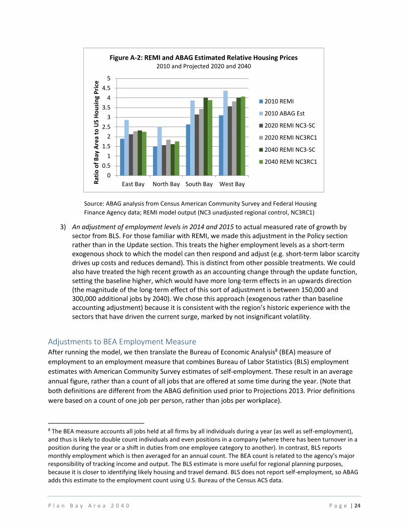
Source: ABAG from Bay Area REMI version 1.7.8, NC3 standard regional output and NC3RC1 capped input and output

2) An adjustment to the ratio of Bay Area relative to national housing prices. This policy variable has a bearing on economic migration levels as these are a function of the attractiveness of the Bay Area amenities and job opportunities, but tempered by the cost of housing. We found that REMI’s account of the cost of housing relative to the U.S. as a whole is substantially lower than what we calculate from other sources, leading to overly optimistic economic migration flows. Our adjustment was created using 2013 five-year American Community Survey (ACS) data for the U.S. and the MSAs relative to our analysis and the FHFA index adjusted to a 2011 base (to be consistent with the five-year ACS data). We used this data to create a series for price by MSA relative to the U.S. In looking back to 1975, it leaves only a small advantage for the Bay Area relative to the U.S., consistent with historic estimates. We then averaged the relative price from 2005 to 2014. We applied 50 percent of the difference between our calculations and the REMI levels to the forecast. As with construction investment, REMI still recalculates the relative price. The effect is insignificant by 2040 but raises prices midway through the forecast, relative to REMI’s unadjusted relative prices, as shown in Figure A-2.

0

20

40

60

80

100

Bill

ion

s o

f fi

xed

(2

00

9)

do

llars

Figure A-1: Residential Investment (Unconstrained and Capped at Historic Peak)

REMI Standard Cap Input Cap Output


Source: ABAG analysis from Census American Community Survey and Federal Housing

Finance Agency data; REMI model output (NC3 unadjusted regional control, NC3RC1)

3) An adjustment of employment levels in 2014 and 2015 to actual measured rate of growth by sector from BLS. For those familiar with REMI, we made this adjustment in the Policy section rather than in the Update section. This treats the higher employment levels as a short-term exogenous shock to which the model can then respond and adjust (e.g. short-term labor scarcity drives up costs and reduces demand). This is distinct from other possible treatments. We could also have treated the high recent growth as an accounting change through the update function, setting the baseline higher, which would have more long-term effects in an upwards direction (the magnitude of the long-term effect of this sort of adjustment is between 150,000 and 300,000 additional jobs by 2040). We chose this approach (exogenous rather than baseline accounting adjustment) because it is consistent with the region’s historic experience with the sectors that have driven the current surge, marked by not insignificant volatility.

Adjustments to BEA Employment Measure After running the model, we then translate the Bureau of Economic Analysis8 (BEA) measure of

employment to an employment measure that combines Bureau of Labor Statistics (BLS) employment

estimates with American Community Survey estimates of self-employment. These result in an average

annual figure, rather than a count of all jobs that are offered at some time during the year. (Note that

both definitions are different from the ABAG definition used prior to Projections 2013. Prior definitions

were based on a count of one job per person, rather than jobs per workplace).

8 The BEA measure accounts all jobs held at all firms by all individuals during a year (as well as self-employment), and thus is likely to double count individuals and even positions in a company (where there has been turnover in a position during the year or a shift in duties from one employee category to another). In contrast, BLS reports monthly employment which is then averaged for an annual count. The BEA count is related to the agency’s major responsibility of tracking income and output. The BLS estimate is more useful for regional planning purposes, because it is closer to identifying likely housing and travel demand. BLS does not report self-employment, so ABAG adds this estimate to the employment count using U.S. Bureau of the Census ACS data.

0

0.5

1

1.5

2

2.5

3

3.5

4

4.5

5

East Bay North Bay South Bay West BayRat

io o

f B

ay A

rea

to U

S H

ou

sin

g P

rice

Figure A-2: REMI and ABAG Estimated Relative Housing Prices2010 and Projected 2020 and 2040

2010 REMI

2010 ABAG Est

2020 REMI NC3-SC

2020 REMI NC3RC1

2040 REMI NC3-SC

2040 REMI NC3RC1


Table A-4 compares the 1.7.8 REMI control with the final forecast, using the BLS plus self-employment

definition of employment. Table A-5 shows the ratios used to adjust BEA to BLS plus self-employment

counts, estimated from an average of 2007, 2010 and 2013.

Table A-4: Bay Area Employment Projections from REMI Standard Control and Final Forecast

2010 2040 2040 Percent Change 2010-2040

(Employment in Thousands) EDD+SE REMI SC Final Forecast

REMI SC Final Forecast

Agriculture & Natural Resources 25.1 24.8 24.4 -1.3% -2.9%

Construction 165.7 411.0 313.4 148.0% 89.1%

Manufacturing & Wholesale 428.5 395.7 408.3 -7.7% -4.7%

Retail 324.8 353.4 398.2 8.8% 22.6%

Transportation & Utilities 97.1 97.1 110.5 -0.1% 13.7%

Information 118.0 114.5 165.0 -2.9% 39.8%

Financial & Leasing 194.9 234.1 234.5 20.1% 20.3%

Professional & Managerial Services 625.2 1062.4 1093.4 69.9% 74.9%

Health & Educational Services 502.7 883.3 887.6 75.7% 76.6%

Arts, Recreation & Other Services 476.5 577.9 591.8 21.3% 24.2%

Government 452.2 474.9 471.3 5.0% 4.2%

Total Jobs 3410.9 4629.0 4698.4 35.7% 37.7% Source: ABAG analysis from Bay Area REMI Model version 1.7.8, standard regional control and NC3RC1

BEA employment numbers are divided by the factors in Table A-5 to give estimates of the BLS

(employment by place of work) plus self-employment equivalent.

Table A-5: Adjustment Ratios: BEA Employment Level Relative to BLS + Self Employment

Employment Sector Adjustment Factor

Agriculture & Natural Resources 1.402484

Construction 1.158725

Manufacturing & Wholesale 1.084723

Retail 1.168494

Transportation & Utilities 1.239593

Information 1.12953

Financial & Leasing 2.377468

Professional & Managerial Services 1.342899

Health & Educational Services 1.091576

Arts, Recreation & Other Services 1.374565

Government 1.035506

Source: ABAG analysis using BEA, BLS and American Community Survey data


Population In developing the preliminary forecast, staff used two separate but similar population modeling

approaches. The Pitkin-Myers population model for the Bay Area uses a cohort survival model, with

careful attention to immigrant status, including generation since immigrating.9 The REMI model uses a

simpler cohort survival model, which also recognizes differences by ethnic group, but assumes once

immigration has happened, the immigrant takes on the characteristics of the ethnic group. We

compared the results of the different models in terms of age and ethnicity and found, especially for age

categories, results were very similar. For consistency with the employment data, we used the REMI

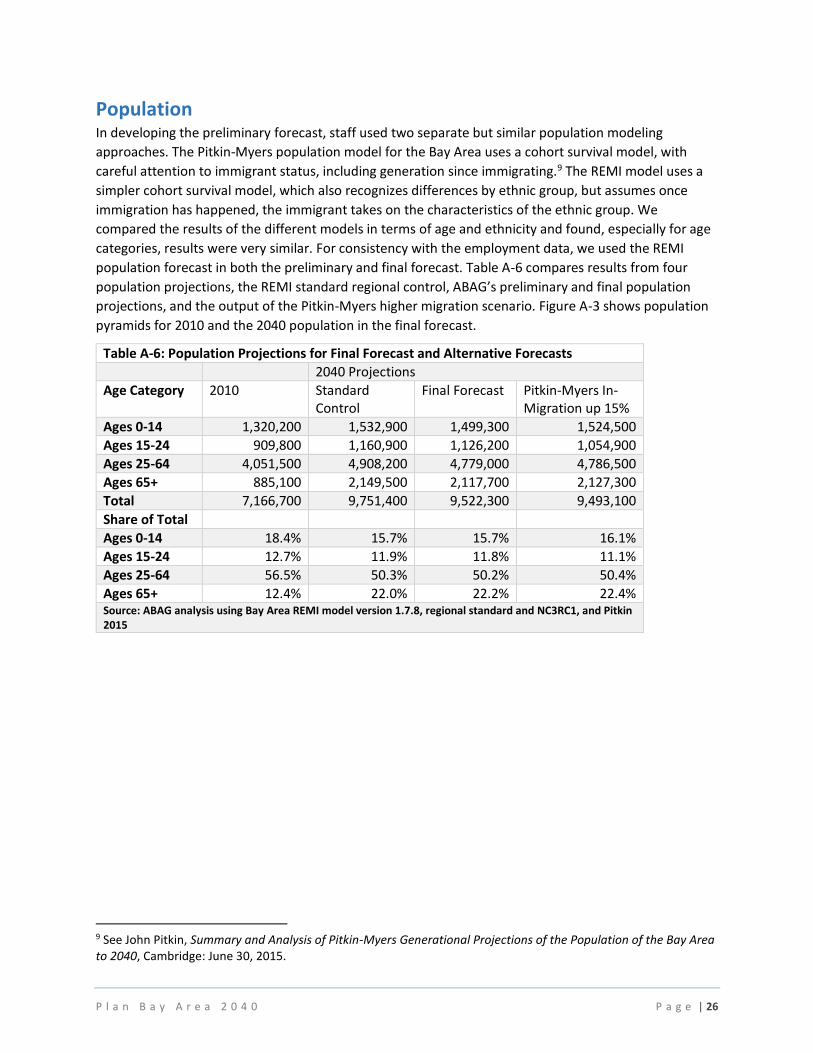
population forecast in both the preliminary and final forecast. Table A-6 compares results from four

population projections, the REMI standard regional control, ABAG’s preliminary and final population

projections, and the output of the Pitkin-Myers higher migration scenario. Figure A-3 shows population

pyramids for 2010 and the 2040 population in the final forecast.

Table A-6: Population Projections for Final Forecast and Alternative Forecasts

2040 Projections

Age Category 2010 Standard Control

Final Forecast Pitkin-Myers In-Migration up 15%

Ages 0-14 1,320,200 1,532,900 1,499,300 1,524,500

Ages 15-24 909,800 1,160,900 1,126,200 1,054,900

Ages 25-64 4,051,500 4,908,200 4,779,000 4,786,500

Ages 65+ 885,100 2,149,500 2,117,700 2,127,300

Total 7,166,700 9,751,400 9,522,300 9,493,100

Share of Total

Ages 0-14 18.4% 15.7% 15.7% 16.1%

Ages 15-24 12.7% 11.9% 11.8% 11.1%

Ages 25-64 56.5% 50.3% 50.2% 50.4%

Ages 65+ 12.4% 22.0% 22.2% 22.4% Source: ABAG analysis using Bay Area REMI model version 1.7.8, regional standard and NC3RC1, and Pitkin 2015

9 See John Pitkin, Summary and Analysis of Pitkin-Myers Generational Projections of the Population of the Bay Area to 2040, Cambridge: June 30, 2015.


Figure A-3: Final Forecast Population Age Distributions, 2010 and 2040

Source: ABAG from US Census and REMI model version 1.7.8, NC3RC1

Household Estimates Household estimates are computed by applying headship rates, or the number of householders relative

to the population calculated from the ACS to the REMI population output by age and ethnicity. The

headship rate is applied to age/race/gender bins: two genders, four race / ethnic groups and 15 age

groups, or a total of 120 distinct groups. Rates are pooled from ACS one-year Public Use Microdata

Sample (PUMS) samples for the years 2006 to 2014, with an exponentially weighted smoothing average

applied to avoid spikes in particular in the thinner slices of the PUMS sample.

While not adjusting headship rates secularly across the board, we did two specific rate adjustments:

1) We marginally reduced headship rates for Black and White, non-Hispanic households, age groups 25-34 and 65-74 by 5 percentage points to reflect expected changes in household sizes for those groups, due to changing cultural and financial conditions.

2) We reduced headship rates for Black and White, non-Hispanic households age groups 75+ by 10 percentage points to reflect expected increases in male survival rates.

We did not adjust headship rates for other ethnic groups related to increased "survival" of older age

groups because headship rates were already so low for those ethnicities. Headship rates are

summarized for the final forecast in Table A-7.

2010 2040

Ages 0-4Ages 5-9

Ages 10-14Ages 15-19Ages 20-24Ages 25-29Ages 30-34Ages 35-39Ages 40-44Ages 45-49Ages 50-54Ages 55-59Ages 60-64Ages 65-69Ages 70-74Ages 75-79Ages 80-84

Ages 85+

8% 6% 4% 2% 0% 2% 4% 6% 8% 8% 6% 4% 2% 0% 2% 4% 6% 8%


Table A-7: Headship Rates by Age, Gender and Ethnicity

gender Females Males

Race/ ethnicity

Black-NonHisp

Hispanic Other-NonHisp

White-NonHisp

Black-NonHisp

Hispanic Other-NonHisp

White-NonHisp

Final Forecast Rates

Age

5-19 0.0079 0.0041 0.0032 0.0063 0.0027 0.0038 0.0038 0.0040

20-24 0.2145 0.1410 0.1333 0.1854 0.1250 0.1051 0.1300 0.1652

25-29 0.4264 0.2917 0.2526 0.3297 0.1976 0.2525 0.3072 0.3195

30-34 0.4996 0.3938 0.3227 0.4241 0.3377 0.3705 0.5099 0.4652

35-39 0.6182 0.4092 0.3304 0.4864 0.4361 0.4514 0.5973 0.5432

40-44 0.6583 0.4296 0.3730 0.5316 0.4815 0.5020 0.6176 0.5557

45-49 0.6676 0.4290 0.3765 0.5238 0.5152 0.5207 0.6094 0.5897

50-54 0.6335 0.4319 0.3626 0.5296 0.5969 0.5389 0.6401 0.6182

55-59 0.6230 0.4450 0.3517 0.5317 0.5985 0.5511 0.6068 0.6427

60-64 0.6590 0.4260 0.3202 0.5450 0.6333 0.5852 0.6062 0.6817

65-69 0.6345 0.3922 0.3161 0.4986 0.6408 0.6314 0.5732 0.6829

70-74 0.6592 0.4589 0.2982 0.5161 0.6724 0.5735 0.5436 0.6862

75-79 0.6206 0.4298 0.3448 0.5016 0.6361 0.6103 0.5636 0.6629

80-84 0.6313 0.5203 0.4176 0.5485 0.6558 0.5400 0.5557 0.6491

85+ 0.6118 0.4394 0.4458 0.6338 0.5327 0.5425 0.5632 0.6622

Income Distribution The income distribution analysis is designed to take into account structural characteristics of the region

including demographic factors such as the age profile and ethnic mix, and economic factors such as the

predominant industries and occupations in which people work, as well as the various sources of income

(retirement income, public assistance income, wage and salary income). Other aspects of Bay Area

regional forecasting rely on estimates of the distribution of income among four income bins originally

defined using 1989 incomes and later updated using 1999 incomes. The categories, originally, were:

1) Below $25,000 (1989 dollars, updated to $30,000 for 1999 dollars) 2) Between $25,000 and $45,000 (1989 dollars, upper break point updated to $60,000 for 1999) 3) Between $45,000 and $75,000 (1989 dollars, upper break point updated to $100,000 for 1999),

and 4) Above $75,000 (1989 dollars, updated to $100,000 for 1999.

As there is much uncertainty surrounding how income distributions change as a function of source

uncertainty (i.e. how the population changes; how firms compensate their workers; how competitive

are the local industries, among other things), the approach used estimates basic relationships between

economic features and the share in a certain range of the income spectrum. All other things equal, for

example, locations with a relatively large share of management occupations may be expected to have


more upper income households, while locations with a higher proportion receiving public assistance

may conversely be expected to have more low-income households. To capture such relationships, ABAG

specified four regression models (using American Community Survey and Census 2000 county-level

data) on the relationship between demographic and economic variables and share of households in

each of the four income quartiles defined above.

The results of these regressions are shown in Tables A-8 to A-11.

Table A-8: Regression Results for Income Category 1 (Households below $30,000, 1999 dollars)

params pvals std test_stats

Adjusted R-Squared 0 0 0 0.669211

R-Squared 0 0 0 0.672062

Intercept 0.741601 4.37E-41 0.052547

Share of population, White (not Hispanic) -0.17261 3.65E-39 0.012572

Wharton Residential Land Use Regulation Index -0.01799 1.35E-10 0.00277

Share of population, 65 and over 0.997485 6.22E-50 0.063133

county housing price median relative to US -0.05317 1.32E-56 0.003127

more than 1 million people in MSA -0.04618 5.23E-27 0.004156

public assistance income, log 0.040692 5.37E-38 0.003015

retirement income, log -0.04888 1.25E-33 0.003884

Share employed in nat resources, construction, and maintenance occupations 0.427559 1.18E-22 0.042505

F Test 235.6765 9.2E-217 0

Table A-9: Regression Results for Income Category 2 (Households $30,000-$59,999, 1999 dollars)

params pvals Std test_stats


R-Squared 0 0 0 0.419768

Intercept 0.530093 4.16E-89 0.023653

Share of population 16 and over in labor force 0.090489 4.74E-05 0.022137

Share of population, Hispanic -0.05252 1E-13 0.00695

Wharton Residential Land Use Regulation Index -0.00256 0.055326 0.001336

Share of population, 25-64 -0.35542 1.14E-14 0.045264

county housing price median relative to US -0.02176 9.58E-35 0.001697

County falls in Census Region 9 0.013903 3.67E-06 0.002985

Share employed in education services -0.32121 1.62E-20 0.033779

Share employed in health care services -0.23159 2.98E-10 0.036355

F Test 83.19669 2.2E-103 0


Table A-10: Regression Results for Income Category 3 (Households $60,000-$99,999, 1999 dollars)



R-Squared 0 0 0 0.650053

Intercept -1.08725 1.94E-61 0.060906

Share of population 16 and over in labor force 0.290893 2.05E-35 0.022443

Share of population, Black (Not Hispanic) -0.03842 7.73E-06 0.008541

Wharton Residential Land Use Regulation Index 0.007572 7.76E-08 0.001398

Share employed in health care services -0.32454 1.88E-17 0.037421

Share employed in professional and scientific services -0.49631 4.73E-26 0.045586

more than 1 million people in MSA 0.019135 2.35E-18 0.002144

per capita income, log 0.115644 3.85E-60 0.006561

F Test 244.4039 4.9E-205 0

Table A-11: Regression Results for Income Category 4 ($100,000 and over, 1999 dollars)



r2 0 0 0 0.799035

Intercept -1.2822 8.17E-55 0.078061 0

county housing price median relative to US 0.028745 1.37E-45 0.001943 0

more than 1 million people in MSA 0.016216 1.72E-16 0.00194 0

per capita income, log 0.134153 1.56E-58 0.007866 0

Share employed in management occupations 0.112038 1.4E-08 0.019613 0

Share employed in services occupations -0.26406 1.23E-13 0.035204 0

F Test 948.6722 0 0 0

The parameters estimated in these regressions are applied to the subregional results of the REMI-based

forecast to estimate future shares of households in each income group. (REMI results are estimated for

four subregions within the Bay Area, including the East Bay—Alameda and Contra Costa counties, North

Bay—Napa, Solano and Sonoma counties, South Bay—Santa Clara County, and West Bay—Marin, San

Francisco and San Mateo Counties.)

Applying regression model coefficients to the projected REMI data for each subregion, we estimate a

time series of future shares in each bin. In reaching these shares, we make a number of normalizing

adjustments:

1) Predicted shares come from four separate regressions that are not constrained to fall in any particular range. The sum of the shares predicted by the four regressions is then normalized to 1.


2) These shares are indexed to the base year, with regression results expressed as changes over time according to the future state of the region as provided by REMI.

3) The indexed amounts are then applied to the base 2010 numbers to reach a growth in households in each income bin over time.

Figure A-4 compares the 2010 income distribution with the distribution in 2040 in the final forecast. The

final forecast has somewhat higher growth in the highest income category, at the expense of growth in

the two middle categories. The lowest income group grows slightly faster than the overall growth rate,

and more quickly than either of the two middle groups, while the slowest growth is in the lower middle

group. Note that in 2010, the upper income group may have been particularly depressed, because of

lower levels of non-wage income in 2010 (e.g. capital gains) and because of depressed earnings related

to incentive pay.

Source: ABAG analysis using projections from REMI model 1.7.8, NC3RC1.

In-Commute and Employed Residents To calculate the change in in-commute, ABAG estimates the change in employed residents and

compares this to the projected growth of employment by place of work. REMI reports “residence

adjusted employment” (RAE), which is the number of BEA defined jobs held by residents. This number is

not a count of people holding jobs. To adjust this number to something closer to persons holding jobs,

we divide the REMI projected RAE by the overall ratio of BEA to BLS plus self-employment jobs (BLS+SE)

in the year, which we term RAEBLSSE. Our net commute estimate for one year is the difference between

BLS+SE and RAEBLSSE. The change in commute, then, is the change in this estimate. Between 2010 and

2040, in our REMI based forecast, this difference increases by 53,000. (We also used an alternate

calculation method, where we compared the projected labor force growth to employment growth,

assuming a steady level of unemployment of around 5 to 5.5 percent during the forecast period. This

0

0.2

0.4

0.6

0.8

1

1.2

2010 2040

Mill

ion

s o

f H

ou

seh

old

s

Figure A-4: Income Distribution, 2010 and Final Forecast 2040

Low

Middle Low

Middle High

High


method gave more representative net commute numbers in the early years, but showed a decrease in

net commuting over the 30-year period. We have chosen to include the higher number that comes from

the RAE approach in estimating the Regional Housing Control Total, to ensure that the concern about

considering the in-commute is met). Compared to the preliminary forecast, higher employment in the

region led to a slightly higher increase in the net in-commute, from 33,000 in the preliminary forecast.

To translate the commute population into households, we referred to the American Community Survey

to estimate workers per household. The American Community Survey five-year data set gives a

representative range of households over a period from 2009 (when housing was less expensive, but

employment was less available) through 2013 (when housing was becoming less available, but

employment and incomes were higher). For that period, average number of employed workers per

household for the region was 1.55, ranging from 1.37 in Marin to 1.64 in San Mateo. When all workers

(employed and not employed) are included, the proportion drops to 1.42. If we assume the workers in-

commuting from outside the region are likely to be below-median-income workers, then the ratio drops

to 1.41. This is a slightly higher ratio than we used in the preliminary forecast, which was based on

employees by place of work per household and included households with no workers and jobs whose

workers may have commuted from outside. The number of in-commuting households is estimated to be

53,000 divided by 1.41, or 37,600, the number used in estimating the in-commute portion of the

Regional Housing Control Total.

Regional Housing Control Total To compute the regional housing control total, we make a fairly simple calculation of housing associated

with the projected number of households, and add to that the housing that would be associated with

the net increase in the in-commute. We use a vacancy rate of 5 percent to translate the 3,389,000

households in 2040 (final forecast) to 3,567,000 housing units. Applying the same 5 percent vacancy rate

to the 37,600 “in-commute” households, we then estimate a need for 39,600 housing units to satisfy the

requirement that the Regional Housing Control Total include housing for the net increase in in-

commuting. The Regional Housing Control Total becomes 3,606,600 housing units (the sum of 3,567,000

and 39,600), an increase of 822,600 units from 2010, or 767,000 from 2015. In comparison, the

preliminary forecast projected 808,000 additional units compared to 2010, and Plan Bay Area 2013

estimated an addition of 660,000 units.

Documents

REGIONAL FORECAST OF JOBS, POPULATION …2040.planbayarea.org/sites/default/files/2017-07/Regional Forecast...Supervisor Nathan Miley Alameda Supervisor Candace Andersen Contra Costa