Regional model for nitrogen fertilization of site-specificrainfed corn in haplustolls of the central Pampas,Argentina

M. C. Gregoret • M. Dıaz Zorita • J. Dardanelli •

R. G. Bongiovanni

Published online: 26 April 2011� Springer Science+Business Media, LLC 2011

Abstract In semi-arid regions, soil water and nitrogen (N) are generally limiting factors

for corn (Zea mays L.) production; hence, implementation of appropriate N fertilization

strategies is needed. The use of precision agriculture practices based on specific site and

crop properties may contribute to a better allocation of fertilizer among management zones

(MZ). The aim of this study was to develop a model for diagnosis of N availability and

recommendation of N fertilizer rates adjusted to MZ for dryland corn crops growing in

Haplustolls. The model considered variability between MZ by including site-specific

variables [soil available water content at sowing (SAW) and Available Nitrogen (soil

available N-NO3 at planting ? applied N, Nd)] using spatial statistical analysis. The study

was conducted in Cordoba, Argentina in Haplustolls and consisted in four field trials of N

fertilizer (range 0–161 kg N ha-1) in each MZ. The MZ were selected based on elevation

maps analysis. Grain yields varied between MZ and increased with larger SAW and Nd at

sowing. Grain responses to Nd and SAW in any MZ were not different between sites,

allowing to fit a regional model whose parameters (Nd, Nd2, SAW, SAW2) contributed

significantly (p \ 0.001) to yield prediction. Agronomical and economically optimum N

rates varied among MZs. However, the spatial variability of optimum N rates among MZs

within sites was not enough to recommend variable N fertilizer rates instead of a uniform

rate. Variable N fertilizer rates should be recommended only if variability in SAW and soil

N among MZ is greater than that found in this work.

M. C. Gregoret (&)Technical Area, AACREA Cordoba Norte, Sarmiento 1236, Ciudad autonoma de Buenos Aires,Argentinae-mail: cgregoret@yahoo.com

M. Dıaz ZoritaCONICET-FAUBA and Merck Crop Bioscience Argentina, Pilar, Argentina

J. Dardanelli � R. G. BongiovanniINTA Manfredi, Cordoba, Argentina

123

Precision Agric (2011) 12:831–849DOI 10.1007/s11119-011-9224-7

Keywords Variable fertilizer rates � Nitrogen � Spatial statistics � Semi-arid regions

AbbreviationsAON Agronomically-optimum N rate

BD Soil bulk density

EC Soil electrical conductivity

EON Economically-optimum N rate

HP High productivity

LP Low productivity

MP Medium productivity

MZ Management zone

Nd Available Nitrogen (soil available N-NO3 at planting ? applied N)

NUEf Agronomic Fertilizer N use efficiency

P Soil extractable phosphorus

PA Precision agriculture

SAW Soil available water content at sowing

SOM Soil organic matter

TN Total soil nitrogen

VRF Variable rates of fertilizer

Introduction

Corn grain yield varies within a field. Hatfield (2000) defined three types of variability

based on the causal factors: (i) natural (soil and topography); (ii) random (precipitation,

temperature and radiation); and (iii) management (fertilization, plant population, etc.). The

interaction of these types of variability generates effects that may not match the physical

limits of the fields, justifying the use of precision agriculture (PA) technology which

involves site-specific or localized management practices. Site-specific management may be

used to improve production and profitability of agricultural systems by adjusting fertilizer

rates to the characteristics of different management zones (MZ), i.e., zones that may differ

in factors such as the type of soil, topography, water and nutrient availability. The analysis

of spatial and temporal variability between MZ within a field reveals the dynamic nature of

soil properties (Cox et al. 2003). In the Pampas region, the difference between high

nitrogen (N) crop demand and the usually limited soil N supply makes N the most limiting

nutrient for corn (Zea mays L.) growth and yield (Andrade et al. 1996). N-fertilizer

application adjusted to MZ requires knowing each MZ’s history of N demand, N-use

efficiency and soil capability to supply a fraction of crop N during the growing season

(Hatfield 2000). Haplustoll soils are representative of the semi-arid Pampas regions, where

water and nutrient availability are usually limiting factors in the production of different

crops (Jarsun et al. 2003).

Integrating diagnosis of N requirements and recommendations for N application into

simple models might be useful for improving N use efficiency and therefore crop profit-

ability. In Rıo Cuarto, Argentina, Anselin et al. (2004) estimated corn crop response to

variations between topographic positions within the field with a quadratic function of N

fertilizer applied. However, as Liu et al. (2006) stated, this model has limitations because it

832 Precision Agric (2011) 12:831–849

123

does not consider soil mineral N availability and soil available water content at sowing

(SAW) at sowing and the interaction of these variables with applied N, because the model

assumes that these variables are inherent to the landscape. Therefore, variability in N and

SAW supply between MZ would be included in the error term. Agronomic fertilization

efficiency in a given environment depends on available soil mineral N and SAW, which

affect soil N use, crop growth and N dynamics (Ruffo and Parsons 2004; Liu et al. 2006;

Miao et al. 2006).

In semi-arid regions, the model developed by Anselin et al. (2004) could be modified by

incorporating site-specific variables with the aim of improving accuracy of the diagnosis of

N availability and recommendation of variable rates of N fertilizer (VRF). For example,

Liu et al. (2006) proposed the explicit inclusion of two categories of site-specific variables

related to N supply and demand for dryland corn crops in sandy loam and loam soils

in Michigan (USA). The former group includes the variables that affect N availability

(i.e., soil organic matter (SOM) content and cation exchange capacity) and the latter

includes variables related to N demand (e.g., radiation). Moreover, in regions with low and

variable rainfall, water stored in the soil profile at sowing might modify the attainable grain

yields and therefore crop management decisions. Under such conditions, the amount of

SAW can sometimes be more important than rainfall during growing season in determining

crop yields (Moeller et al. 2009).

Recent studies evaluating corn N fertilization models have not included soil N and

SAW, nor discriminated between MZ or used analytical methods that consider spatial

structure of geo-referenced data. The aim of this study was to develop a model for diag-

nosis of N availability and recommendation of N fertilizer rates adjusted to MZ for dryland

corn crops growing in Haplustolls. This model includes soil N and SAW and uses spatial

statistical analysis.

Materials and methods

Experimental sites and general characterization of the study area

The study was performed at four sites located in the semi-arid Pampas region of

Argentina: Site I: 63�420 W, 31�510 S, Site II: 63�410 W, 31�220 S, Site III: 63�430 W,

31�5301.800 S and Site IV: 64�200 W, 31�340 S. Crops at sites I and II were sown in the

2004–2005 crop season; and at sites III and IV, in the 2005–2006 season. The climate in

Table 1 Summary of rainfall and temperatures recorded during the crop cycle in each site

Sites SAW Dates Planting—flowering

Flowering—phys. mat

Planting—phys. mat.

Planting Flowering Physiologicalmaturity

pp T� pp T� pp T�

I 75.25 14/10/04 29/12/04 01/03/05 222 19.7 318 21 540 20.35

II 140.73 14/09/04 05/12/04 01/02/05 249 19.9 175 23 424 21.3

III 181.63 20/10/05 08/01/06 17/03/06 284 20.9 322 21.15 606 21.02

IV 242.65 14/11/05 15/01/06 31/03/06 356 22.8 274 22.4 630 22.6

SAW soil available water (mm), pp precipitation (mm), T� average temperature in �C

Precision Agric (2011) 12:831–849 833

123

the region is mesothermal, with a mean annual rainfall of 750 mm and monsoon-type

distribution (93% of the rainfall events occur between September and April). A summary

of rainfall and temperatures recorded during the crop cycle is shown in Table 1. The

main soil types are Typic Haplustolls with silty loam texture (16% of clay, 68% of silt

and 16% of sand) and with moderate to low SOM content (1.25–3.0%). The soil type of

all MZ in the four sites was classified as Typic Haplustoll of the Oncativo series (Jarsun

et al. 2003).

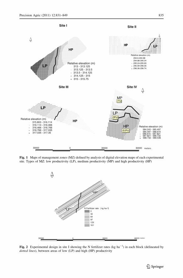
Management zones delimitation

In each site, MZ were delimited based on the analysis of digital elevation maps, which

provide background information about the productivity and soil properties, both influ-

enced by climate and topography (Moore et al. 1993; Vieira et al. 2006). Yield maps

were available from the sites I and II and they were also taken into account for the

delimitation of the MZ. The MZ were identified using the software Management Zone

Analyst (Mizzou-ARS 2000). Management Zone Analyst (MZA) is a decision-aid for

creating within-field management zones based on quantitative field information. It mathe-

matically breaks up a field into natural clusters or zones based on the classification

parameters which allows unsupervised fuzzy clustering of information. The procedure was

unsupervised because it does not require prior knowledge of the classification variables but

it produces natural groupings of data. It is also fuzzy because it allows the classification of

data belonging to different groups. The software, after pooling the data, estimates two

performance indices in order to guide the decision as to which is the best number of groups

or MZ. These indices are the ‘‘normal rate of entropy (NCE)’’, which accounts for the

disruption created by grouping the data into zones and the ‘‘fuzzy performance index

(FPI)’’, which reports the number of members shared between classes. The best data

grouping is the size of area where both indices have their minimum value (Fridgen et al.

2004).

In each of the sites, in order to identify the MZ, ground elevation was surveyed by

collecting positioning data (latitude and longitude) and elevation (m) with a Trimble�

GPS model 4600LS during the winter fallow prior to planting crops. The recording

equipment was placed on a vehicle, which traversed the site in equi-distant transects

every 10 m and an elevation map was made by interpolation to a regular grid of 5 m by

the method of equi-distance kriging. Elevation was represented in contour maps of

curves using the software Surfer version 8.4 (Surface Mapping System, copyright

1993–2003, Golden Software, Inc., USA). Then these elevation logs, processed with the

available yield maps, were entered into the MZA software for classification into

homogeneous groups according to the performance indices described. From this pro-

cedure, the following zones were identified: (i) a high productivity (HP) area, located in

a zone of lower than average elevation, and (ii) a low productivity (LP) zone located at

higher than average elevation (Fig. 1). In site IV, three MZ were identified because they

represented different topographic attributes: (i) a HP MZ located on a plateau higher

than the field mean elevation, with almost no slope (0.9%), (ii) a medium productivity

(MP) area with an elevation below the field mean value and with a slope of 1%, and

(iii) a LP area with an elevation lower than the field mean value, and with a steep slope

of 9%.

834 Precision Agric (2011) 12:831–849

123

HP LP

294.6-294.88294.88-295.24295.24-295.69295.69-296.06296.06-296.74

Relative elevation (m)

Relative elevation (m)

Relative elevation (m)

Relative elevation (m)

LP

LP

HP

HP

313 - 313.125313.125 - 313.5313.5 - 314.125314.125 - 315315 - 315.75

315.803 - 316.114316.114 - 316.466316.466 - 316.766316.766 - 317.035317.035 - 317.35

584.245 - 585.497585.497 - 586.615586.615 - 587.821587.821 - 588.732588.732 - 589.536

600003000030000 0

HP

LP

MP

Fig. 1 Maps of management zones (MZ) defined by analysis of digital elevation maps of each experimentalsite. Types of MZ: low productivity (LP), medium productivity (MP) and high productivity (HP)

"HP"

"LP"

N

Fig. 2 Experimental design in site I showing the N fertilizer rates (kg ha-1) in each block (delineated bydotted lines), between areas of low (LP) and high (HP) productivity

Precision Agric (2011) 12:831–849 835

123

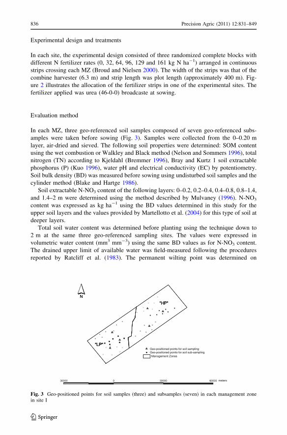
Experimental design and treatments

In each site, the experimental design consisted of three randomized complete blocks with

different N fertilizer rates (0, 32, 64, 96, 129 and 161 kg N ha-1) arranged in continuous

strips crossing each MZ (Broud and Nielsen 2000). The width of the strips was that of the

combine harvester (6.3 m) and strip length was plot length (approximately 400 m). Fig-

ure 2 illustrates the allocation of the fertilizer strips in one of the experimental sites. The

fertilizer applied was urea (46-0-0) broadcaste at sowing.

Evaluation method

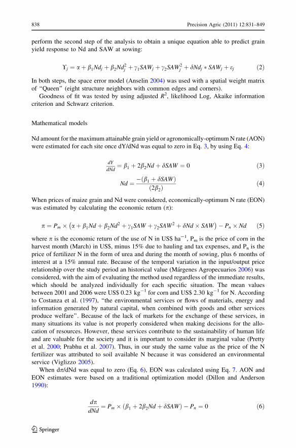
In each MZ, three geo-referenced soil samples composed of seven geo-referenced subs-

amples were taken before sowing (Fig. 3). Samples were collected from the 0–0.20 m

layer, air-dried and sieved. The following soil properties were determined: SOM content

using the wet combustion or Walkley and Black method (Nelson and Sommers 1996), total

nitrogen (TN) according to Kjeldahl (Bremmer 1996), Bray and Kurtz 1 soil extractable

phosphorus (P) (Kuo 1996), water pH and electrical conductivity (EC) by potentiometry.

Soil bulk density (BD) was measured before sowing using undisturbed soil samples and the

cylinder method (Blake and Hartge 1986).

Soil extractable N-NO3 content of the following layers: 0–0.2, 0.2–0.4, 0.4–0.8, 0.8–1.4,

and 1.4–2 m were determined using the method described by Mulvaney (1996). N-NO3

content was expressed as kg ha-1 using the BD values determined in this study for the

upper soil layers and the values provided by Martellotto et al. (2004) for this type of soil at

deeper layers.

Total soil water content was determined before planting using the technique down to

2 m at the same three geo-referenced sampling sites. The values were expressed in

volumetric water content (mm3 mm-3) using the same BD values as for N-NO3 content.

The drained upper limit of available water was field-measured following the procedures

reported by Ratcliff et al. (1983). The permanent wilting point was determined on

"LP"

"HP"

N

"LP"

"HP"

N

"LP"

"HP"

N

Geo-positioned points for soil sampling Geo-positioned points for soil sub-sampling

meters

Fig. 3 Geo-positioned points for soil samples (three) and subsamples (seven) in each management zonein site I

836 Precision Agric (2011) 12:831–849

123

disturbed samples with a -1.5 MPa suction pressure membrane (Richards 1947). SAW

was calculated as the difference between the observed soil water content and that corre-

sponding to permanent wilting point for each soil layer down to 2 m. Soil properties of the

MZ within each site were compared with ANOVA, using InfoStat statistical software

(Infostat 2007).

Because the spatial density of the soil sampling was much lower than grain yield data, it

was necessary to adjust the density of data; thus interpolated soil data were obtained using

the nearest neighbor method following the approach proposed by Griffin et al. (2005). As

explained by these authors, the nearest neighbor interpolation was created by surrounding

each input point by an area such that any location within that area is closer to the original

point than any other point. In this work, depending on the size of a site and the distribution

of soil sampling, each soil sample spanned from 14 to 18% of the total yield data for each

site.

Grain yield evaluation

Yield data were collected with a standard AgLeaderTM yield monitor, a geo-positioned

device located on the combine harvester that measures and records crop yields on-the-go.

Combine speed and GPS were monitored during yield data collection. Grain yield data

were spatially located and analyzed with SSToolbox GIS software (SST 2006). The data

points located approximately 20 m from the borders of the sites were deleted before the

analysis because the combine was unlikely to be full. Finally, the remaining data were

filtered using GeoDa software (Anselin 2004).

To normalize the distance of the observations within and between the strips, the pooled

data from each site (2 111, 1 771, 1 341 and 939 observations at sites I, II, III and IV,

respectively) were arranged in a 6.3 m 9 6.3 m grid averaging the observations within

each polygon. From the resulting square (1 297; 1 049; 1 012 and 588 at sites I, II, III and

IV, respectively), a matrix of spatial weights, weighting the data according to the proximity

between observations, was calculated.

Data analysis

Spatial statistical analysis (Anselin 1988) was performed using the Geoda software

(Anselin 2004). The analysis involved two steps. First the feasibility of integrating each

experimental site into a single response function was determined estimating whether the

response to available Nitrogen (soil available N-NO3 at planting ? applied N) (Nd) was

dependent on geographical location or only on MZ, regardless of the experimental site.

This analysis was based on the following model:

!ij ¼ aþ b1Nd þ b2Nd2 þ c1SAW þ c2SAW2 þ dC þ /Nd � C þ jSAW � C þ mNd� SAW � C þ eij ð1Þ

where Yij is the maize grain yield (kg ha-1) in each experimental site ‘‘C’’ (i) and each geo-

referenced location (j), dCi is a dummy variable for the sites, a, b1, b2, c1, c2, d, x, j and mare the parameters of the regression equation, and eij is the error term of the regression. If

dCi was not significantly different between experimental sites, then it was feasible to

Precision Agric (2011) 12:831–849 837

123

perform the second step of the analysis to obtain a unique equation able to predict grain

yield response to Nd and SAW at sowing:

!j ¼ aþ b1Ndj þ b2Nd2j þ c1SAWj þ c2SAW2

j þ dNdj � SAWj þ ej ð2Þ

In both steps, the space error model (Anselin 2004) was used with a spatial weight matrix

of ‘‘Queen’’ (eight structure neighbors with common edges and corners).

Goodness of fit was tested by using adjusted R2, likelihood Log, Akaike information

criterion and Schwarz criterion.

Mathematical models

Nd amount for the maximum attainable grain yield or agronomically-optimum N rate (AON)

were estimated for each site once dY/dNd was equal to zero in Eq. 3, by using Eq. 4:

dY

dNd¼ b1 þ 2b2Nd þ dSAW ¼ 0 ð3Þ

Nd ¼ � b1 þ dSAWð Þ2b2ð Þ ð4Þ

When prices of maize grain and Nd were considered, economically-optimum N rate (EON)

was estimated by calculating the economic return (p):

p ¼ Pm � aþ b1Nd þ b2Nd2 þ c1SAW þ c2SAW2 þ dNd � SAW� �

� Pn � Nd ð5Þ

where p is the economic return of the use of N in US$ ha-1, Pm is the price of corn in the

harvest month (March) in US$, minus 15% due to hauling and tax expenses, and Pn is the

price of fertilizer N in the form of urea and during the month of sowing, plus 6 months of

interest at a 15% annual rate. Because of the temporal variation in the input/output price

relationship over the study period an historical value (Margenes Agropecuarios 2006) was

considered, with the aim of evaluating the method used regardless of the immediate results,

which should be analyzed individually for each specific situation. The mean values

between 2001 and 2006 were US$ 0.23 kg-1 for corn and US$ 2.30 kg-1 for N. According

to Costanza et al. (1997), ‘‘the environmental services or flows of materials, energy and

information generated by natural capital, when combined with goods and other services

produce welfare’’. Because of the lack of markets for the exchange of these services, in

many situations its value is not properly considered when making decisions for the allo-

cation of resources. However, these services contribute to the sustainability of human life

and are valuable for the society and it is important to consider its marginal value (Pretty

et al. 2000; Prabhu et al. 2007). Thus, in our study the same value as the price of the N

fertilizer was attributed to soil available N because it was considered an environmental

service (Viglizzo 2005).

When dp/dNd was equal to zero (Eq. 6), EON was calculated using Eq. 7. AON and

EON estimates were based on a traditional optimization model (Dillon and Anderson

1990):

dpdNd¼ Pm � b1 þ 2b2Nd þ dSAWð Þ � Pn ¼ 0 ð6Þ

838 Precision Agric (2011) 12:831–849

123

Nd ¼ Pn

Pm

� �� b1 � dSAW

� �� 1

2b2

� �ð7Þ

For each MZ, data of SAW replications were used to calculate AON and EON. Mean

values obtained were compared between MZ within each site using ANOVA.

The response curves of corn grain yield to Nd used in each MZ were estimated with

Eq. 2 using the SAW average value from each MZ. In each site and MZ, Agronomic

fertilizer N-use efficiency (NUEf) was calculated from the difference between corn grain

yield at AON and without N fertilizer, using the following equation (Eq. 8)

NUEf ¼ ðYAON � YNf 0Þ=NfAON ð8Þ

where, YAON is the yield at AON, YNf0 is the yield without N fertilizer and NfAON is the N

fertilizer rate at AON.

At each site, the apparent contribution of variable N fertilizer rates between MZ was

compared against uniform N fertilizer using the average of Nd and SAW information

without discriminating between MZ. Finally, ANOVA and LSD-T analysis were per-

formed for the comparison between both fertilizer strategies with four replicates (each of

the sites).

Results and discussion

Soil properties at the sites

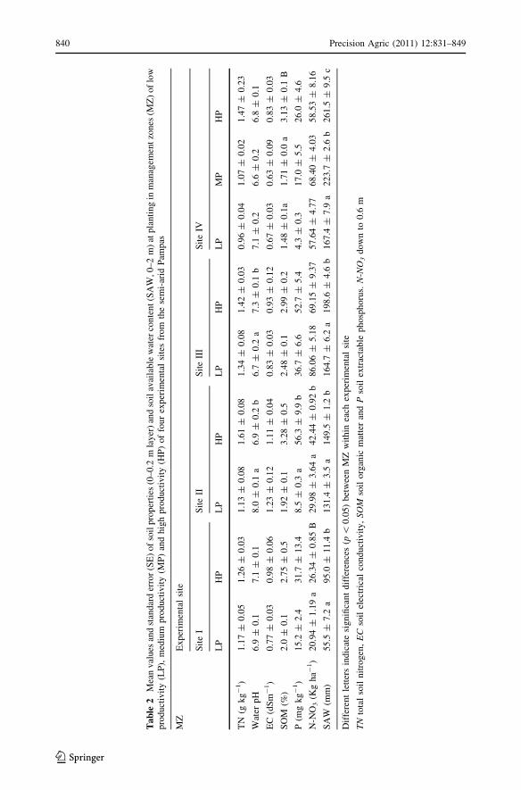
Mean values of soil P, SOM and TN content in the 0–0.2 m soil layer and total SAW in the

0–2 m soil profile at planting were highest in the HP MZ of each site (Table 2) with

statistically significant differences only in some cases. Moreover, N-NO3 content in the

upper 0.6 m layer was similar between MZ, except in site I and II, where SAW differences

between MZ were the greatest (Table 2). The differences in soil properties found between

MZ agree with previous reports. Zubillaga et al. (2006), based on grid sampling of Typic

and Entic Hapludolls from Buenos Aires province (Argentina), observed that the spatial

distribution of some soil properties was not random. Furthermore, they observed that areas

with high crop productivity also showed greater soil TN and greater SAW than LP areas.

The soil properties observed in this study are within the normal range of cropped soils of

the semi-arid Pampas region. Kravchenko and Bullock (2000) used a regression analysis in

Haplaquolls and Argiudolls from central Illinois (USA) and eastern Indiana (USA) and

concluded that differences in the topography explained 30% of the variability in SOM

content and in extractable soil P and K. Likewise, Dharmakeerthi et al. (2005) reported that

more soil N was available in a Typic Hapludalf from Ontario (Canada) at lower positions

in the landscape. The present study agrees with these results, most soil N-NO3 at sowing

was available in the HP MZ, usually at low positions in the field (Table 2).

Distribution of soil water content down the profile (0–2 m in depth) at sowing showed

similar patterns in all MZ of each site (Fig. 4), but the accumulated content differed

between MZ (Table 2), showing a close relationship with the differences in crop pro-

ductivity between MZ (Fig. 6). SAW in LP MZ was 42, 12, 18 and 34 less than in the HP

MZ, in sites I, II, III and IV, respectively. For the same sites, yields were 9, 10, 7, and 26%

larger in HP MZ than in LP ones. According to Moore et al. (1993) and Vieira et al. (2006),

the differences described in SAW amount are associated with a greater water recharge

during fallow in HP MZ due to topographic characteristics. Different soil N and SAW

Precision Agric (2011) 12:831–849 839

123

Ta

ble

2M

ean

val

ues

and

stan

dar

der

ror

(SE

)o

fso

ilp

rop

erti

es(0

–0

.2m

lay

er)

and

soil

avai

lab

lew

ater

con

ten

t(S

AW

,0

–2

m)

atp

lanti

ng

inm

anag

emen

tzo

nes

(MZ

)o

flo

wp

rod

uct

ivit

y(L

P),

med

ium

pro

duct

ivit

y(M

P)

and

hig

hp

rod

uct

ivit

y(H

P)

of

fou

rex

per

imen

tal

site

sfr

om

the

sem

i-ar

idP

amp

as

MZ

Ex

per

imen

tal

site

Sit

eI

Sit

eII

Sit

eII

IS

ite

IV

LP

HP

LP

HP

LP

HP

LP

MP

HP

TN

(gk

g-

1)

1.1

7±

0.0

51

.26

±0

.03

1.1

3±

0.0

81

.61

±0

.08

1.3

4±

0.0

81

.42

±0

.03

0.9

6±

0.0

41

.07

±0

.02

1.4

7±

0.2

3

Wat

erp

H6

.9±

0.1

7.1

±0

.18

.0±

0.1

a6

.9±

0.2

b6

.7±

0.2

a7

.3±

0.1

b7

.1±

0.2

6.6

±0

.26

.8±

0.1

EC

(dS

m-

1)

0.7

7±

0.0

30

.98

±0

.06

1.2

3±

0.1

21

.11

±0

.04

0.8

3±

0.0

30

.93

±0

.12

0.6

7±

0.0

30

.63

±0

.09

0.8

3±

0.0

3

SO

M(%

)2

.0±

0.1

2.7

5±

0.5

1.9

2±

0.1

3.2

8±

0.5

2.4

8±

0.1

2.9

9±

0.2

1.4

8±

0.1

a1

.71

±0

.0a

3.1

3±

0.1

B

P(m

gk

g-

1)

15

.2±

2.4

31

.7±

13

.48

.5±

0.3

a5

6.3

±9

.9b

36

.7±

6.6

52

.7±

5.4

4.3

±0

.31

7.0

±5

.52

6.0

±4

.6

N-N

O3

(Kg

ha-

1)

20

.94

±1

.19

a2

6.3

4±

0.8

5B

29

.98

±3

.64

a4

2.4

4±

0.9

2b

86

.06

±5

.18

69

.15

±9

.37

57

.64

±4

.77

68

.40

±4

.03

58

.53

±8

.16

SA

W(m

m)

55

.5±

7.2

a9

5.0

±1

1.4

b1

31

.4±

3.5

a1

49

.5±

1.2

b1

64

.7±

6.2

a1

98

.6±

4.6

b1

67

.4±

7.9

a2

23

.7±

2.6

b2

61

.5±

9.5

c

Dif

fere

nt

lett

ers

ind

icat

esi

gn

ifica

nt

dif

fere

nce

s(p

\0

.05)

bet

wee

nM

Zw

ith

inea

chex

per

imen

tal

site

TN

tota

lso

iln

itro

gen

,E

Cso

ilel

ectr

ical

con

duct

ivit

y,

SO

Mso

ilo

rgan

icm

atte

ran

dP

soil

extr

acta

ble

phosp

horu

s.N

-NO

3d

ow

nto

0.6

m

840 Precision Agric (2011) 12:831–849

123

combinations determined different environments for maize production. In Typic Fragi-

ochrepts from the state of New York (USA), Timlin et al. (1998) found that soil water

availability, either in excess or deficit is a source of corn grain variability.

Site IISite I

Site IVSite III

-2

-1,5

-1

-0,5

Volumetric Water Content

(mm3 mm-3)

Dep

th (

m)

LP HP´-1.5MPa DUL

0

-2

-1,5

-1

-0,5

Volumetric Water Content

(mm3 mm-3)

Dep

th (

m)

LP HP´-1.5MPa DULMP

0

-2

-1,5

-1

-0,5

Volumetric Water Content

(mm3 mm-3)

Dep

th (

m)

LP HP´-1.5MPa DUL

0

-2

-1,5

-1

-0,5

0 100 200 300 400 0 100 200 300 400

0 100 200 300 400 0 100 200 300 400

Volumetric Water Content

(mm3 mm-3)

Dep

th (

m)

LP HP´-1.5MPa DUL

0

Fig. 4 Volumetric soil water content (0–2 m depth) at planting in management zones of low (LP), medium(MP) and high (HP) productivity of four sites from the semi-arid Pampas. The dashed lines indicate thevolumetric soil water content at the drained upper limit (DUL) and the solid lines indicate the volumetricsoil water content measured in the laboratory at -1.5 MPa water potential. The horizontal bars show thestandard errors of the mean

Precision Agric (2011) 12:831–849 841

123

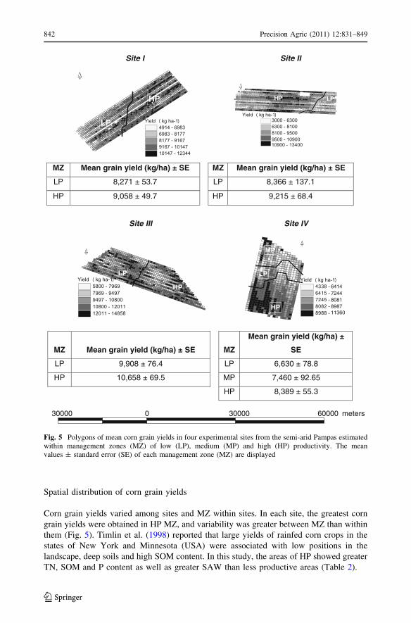
Spatial distribution of corn grain yields

Corn grain yields varied among sites and MZ within sites. In each site, the greatest corn

grain yields were obtained in HP MZ, and variability was greater between MZ than within

them (Fig. 5). Timlin et al. (1998) reported that large yields of rainfed corn crops in the

states of New York and Minnesota (USA) were associated with low positions in the

landscape, deep soils and high SOM content. In this study, the areas of HP showed greater

TN, SOM and P content as well as greater SAW than less productive areas (Table 2).

Site I Site II

N

LP

HP

MZ Mean grain yield (kg/ha) ± SE MZ Mean grain yield (kg/ha) ± SE

LP 8,271 ± 53.7 LP 8,366 ± 137.1

Site III Site IV

N

LP

HP

N

MP

LP

HP

MZ Mean grain yield (kg/ha) ± SE MZ

Mean grain yield (kg/ha) ±

SE

LP 9,908 ± 76.4 LP 6,630 ± 78.8

HP 9,058 ± 49.7 HP 9,215 ± 68.4

HP 10,658 ± 69.5 MP 7,460 ± 92.65

8,389 ± 55.3PH

30000 0 30000 60000 meters

N

HP LP

Fig. 5 Polygons of mean corn grain yields in four experimental sites from the semi-arid Pampas estimatedwithin management zones (MZ) of low (LP), medium (MP) and high (HP) productivity. The meanvalues ± standard error (SE) of each management zone (MZ) are displayed

842 Precision Agric (2011) 12:831–849

123

The model performed well among MZ within sites. Goodness of fit tests (adjusted R2,

likelihood Log, Akaike information criterion and Schwarz criterion), were (p \ 0.05).

Thus, all MZs and site data sets were pooled and a unique model was tested. Table 3

summarizes the coefficients between yields and Nd amount, SAW and the dummy vari-

ables for each site estimated using the model fitted with Eq. 1. The coefficients of the

Table 3 Summary of the coef-ficients and standard errors esti-mated to the response of soilavailable N (Nd) (soil availableN-NO3 ? fertilizer N down to0.6 m) and soil available water(SAW) down to 2 m, withdummy variables for all themanagement zones (MZ) withineach experimental site (I, II, IIIand IV) in rainfed corn crops,during 2004–2005 and2005–2006, in the semi-aridPampas

Standard errors (SE) andsignificance probability levels(p) \ 0.10 are displayed, NS non-significant (p [ 0.10)

Variable Coefficient SE p

Constant 8 417.65 5 775.3 NS

Nd 33.93 1.9 0.001

Nd2 -0.07 0 0.001

SAW -25.43 82.2 NS

SAW2 0.06 0.3 NS

I -4 482.31 5 806.7 NS

II -8 036.48 – –

III 10 934.40 10 806.8 NS

IV 1 584.30 5 961.8 NS

Nd 9 I 0.64 3.2 NS

Nd 9 II 8.49 – –

Nd 9 III 10.51 6.5 0.001

Nd 9 IV -19.65 5.1 0.001

Nd2 9 I -0.05 0 0.001

Nd2 9 II 0.04 – –

Nd2 9 III 0.04 0 0.001

Nd2 9 IV 0.05 0 0.001

SAW 9 I 83.02 83.2 NS

SAW 9 II 62.83 – –

SAW 9 III -122.2 135.2 NS

SAW 9 IV -23.65 82.6 NS

SAW2 9 I -0.42 0.3 NS

SAW2 9 II -0.1 – –

SAW2 9 III 0.47 0.4 NS

SAW2 9 IV 0.07 0.3 NS

Nd 9 SAW 9 I 0.1 0 0.001

Nd 9 SAW 9 II 0.06 – –

Nd 9 SAW 9 III -0.18 0 0.001

Nd 9 SAW 9 IV 0.01 0 NS

k 0.57 0 0.001

Goodnes of fit measures

Adjusted R2 0.69

Likelihood Log -31 416.5

Akaike information criterion (AIC) 62 878.9

Schwarz criterion (SC) 63 022.3

Test of the likelihood ratio 926.8

Precision Agric (2011) 12:831–849 843

123

dummy variables were not statistically significant, suggesting that grain responses to Nd

and SAW in any MZ were not different between sites. Then, under the conditions used in

the present study, the site-specific variables (Nd and SAW) were equally related to yield,

independent of the location of the sites.

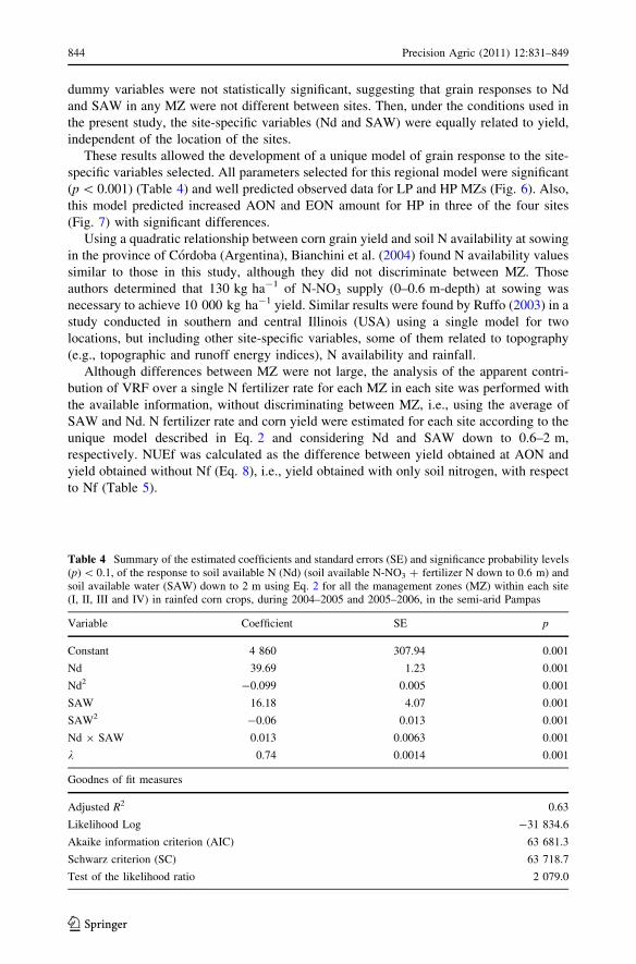
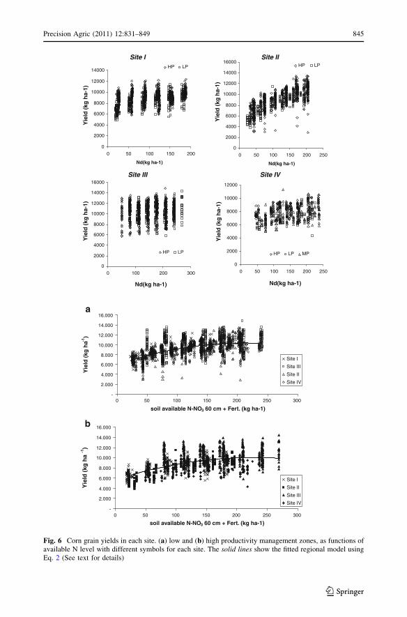
These results allowed the development of a unique model of grain response to the site-

specific variables selected. All parameters selected for this regional model were significant

(p \ 0.001) (Table 4) and well predicted observed data for LP and HP MZs (Fig. 6). Also,

this model predicted increased AON and EON amount for HP in three of the four sites

(Fig. 7) with significant differences.

Using a quadratic relationship between corn grain yield and soil N availability at sowing

in the province of Cordoba (Argentina), Bianchini et al. (2004) found N availability values

similar to those in this study, although they did not discriminate between MZ. Those

authors determined that 130 kg ha-1 of N-NO3 supply (0–0.6 m-depth) at sowing was

necessary to achieve 10 000 kg ha-1 yield. Similar results were found by Ruffo (2003) in a

study conducted in southern and central Illinois (USA) using a single model for two

locations, but including other site-specific variables, some of them related to topography

(e.g., topographic and runoff energy indices), N availability and rainfall.

Although differences between MZ were not large, the analysis of the apparent contri-

bution of VRF over a single N fertilizer rate for each MZ in each site was performed with

the available information, without discriminating between MZ, i.e., using the average of

SAW and Nd. N fertilizer rate and corn yield were estimated for each site according to the

unique model described in Eq. 2 and considering Nd and SAW down to 0.6–2 m,

respectively. NUEf was calculated as the difference between yield obtained at AON and

yield obtained without Nf (Eq. 8), i.e., yield obtained with only soil nitrogen, with respect

to Nf (Table 5).

Table 4 Summary of the estimated coefficients and standard errors (SE) and significance probability levels(p) \ 0.1, of the response to soil available N (Nd) (soil available N-NO3 ? fertilizer N down to 0.6 m) andsoil available water (SAW) down to 2 m using Eq. 2 for all the management zones (MZ) within each site(I, II, III and IV) in rainfed corn crops, during 2004–2005 and 2005–2006, in the semi-arid Pampas

Variable Coefficient SE p

Constant 4 860 307.94 0.001

Nd 39.69 1.23 0.001

Nd2 -0.099 0.005 0.001

SAW 16.18 4.07 0.001

SAW2 -0.06 0.013 0.001

Nd 9 SAW 0.013 0.0063 0.001

k 0.74 0.0014 0.001

Goodnes of fit measures

Adjusted R2 0.63

Likelihood Log -31 834.6

Akaike information criterion (AIC) 63 681.3

Schwarz criterion (SC) 63 718.7

Test of the likelihood ratio 2 079.0

844 Precision Agric (2011) 12:831–849

123

II etiS I etiS

0

2000

4000

6000

8000

10000

12000

14000

Nd(kg ha-1)

Yie

ld (

kg h

a-1)

HP LP

0

2000

4000

6000

8000

10000

12000

14000

16000

Nd(kg ha-1)

Yie

ld (

kg h

a-1)

HP LP

VI etiS III etiS

0

2000

4000

6000

8000

10000

12000

14000

16000

Nd(kg ha-1)

Yie

ld (

kg h

a-1)

HP LP

0

2000

4000

6000

8000

10000

12000

Nd(kg ha-1)

Yie

ld (

kg h

a-1)

HP LP MP

a

-

2.000

4.000

6.000

8.000

10.000

12.000

14.000

16.000

soil available N-NO3 60 cm + Fert. (kg ha-1)

Yie

ld (

kg h

a-1)

Site I

Site III

Site II

Site IV

b

-

2.000

4.000

6.000

8.000

10.000

12.000

14.000

16.000

0 50 100 150 200 0 50 100 150 200 250

0 100 200 300 0 50 100 150 200 250

0 50 100 150 200 250 300

0 50 100 150 200 250 300

soil available N-NO3 60 cm + Fert. (kg ha-1)

Yie

ld (

kg h

a-1

)

Site I

Site II

Site III

Site IV

Fig. 6 Corn grain yields in each site. (a) low and (b) high productivity management zones, as functions ofavailable N level with different symbols for each site. The solid lines show the fitted regional model usingEq. 2 (See text for details)

Precision Agric (2011) 12:831–849 845

123

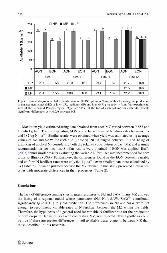
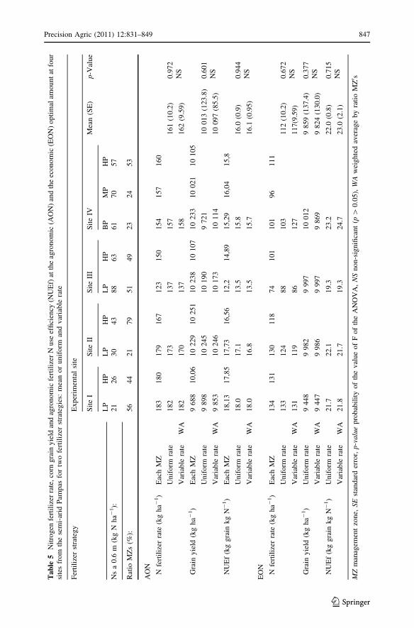
Maximum yield estimated using data obtained from each MZ varied between 9 853 and

10 246 kg ha-1. The corresponding AON would be achieved at fertilizer rates between 137

and 182 kg Nf ha-1. Similar results were obtained when yield was estimated using average

values of Nd and SAW for each site (Table 5). NUEf ranged between 13 and 18 kg of

grain (kg of applied N) considering both the relative contribution of each MZ and a single

recommendation per location. Similar results were obtained if EON was applied. Ruffo

(2003) found similar results evaluating the variable N fertilizer rate recommended for corn

crops in Illinois (USA). Furthermore, the differences found in the EON between variable

and uniform N fertilizer rates were only 0.4 kg ha-1, even smaller than those calculated by

us (Table 5). It can be justified because the MZ defined in this study presented similar soil

types with moderate differences in their properties (Table 2).

Conclusions

The lack of differences among sites in grain responses to Nd and SAW in any MZ allowed

the fitting of a regional model whose parameters (Nd, Nd2, SAW, SAW2) contributed

significantly (p \ 0.001) to yield prediction. The differences in Nd and SAW were not

enough to recommend variable rates of N fertilizer between the MZ within the fields.

Therefore, the hypothesis of a general need for variable N fertilizer rate for the production

of corn crops in Haplustoll soil with contrasting MZ, was rejected. This hypothesis could

be true if there are greater differences in soil available water contents between MZ than

those described in this research.

0

50

100

150

200

250A

vaila

ble

N (

kg h

a-1

)HP MP LP

HP 207 158 210 161 214 164 217 168

MP 215 166

LP 204 155 209 160 211 162 212 163

AON EON AON EON AON EON AON EON

Site I Site II Site III Site IV

a a a b

a b a b a b

a b

a b c

a b c

Fig. 7 Estimated agronomic (AON) and economic (EON) optimum N availability for corn grain productionin management zones (MZ) of low (LP), medium (MP) and high (HP) productivity from four experimentalsites of the semi-arid Pampas region. Different letters at the top of each column for each site indicatesignificant differences (p \ 0.05) between MZ

846 Precision Agric (2011) 12:831–849

123

Tab

le5

Nit

rog

enfe

rtil

izer

rate

,co

rng

rain

yie

ldan

dag

ron

om

icfe

rtil

izer

Nu

seef

fici

ency

(NU

Ef)

atth

eag

ron

om

ic(A

ON

)an

dth

eec

on

om

ic(E

ON

)o

pti

mal

amo

un

tat

fou

rsi

tes

fro

mth

ese

mi-

arid

Pam

pas

for

two

fert

iliz

erst

rate

gie

s:m

ean

or

un

ifo

rman

dv

aria

ble

rate

Fer

tili

zer

stra

teg

yE

xp

erim

enta

lsi

te

Sit

eI

Sit

eII

Sit

eII

IS

ite

IVM

ean

(SE

)p-V

alu

e

LP

HP

LP

HP

LP

HP

BP

MP

HP

Ns

a0

.6m

(kg

Nh

a-1):

21

26

30

43

88

63

61

70

57

Rat

ioM

Zs

(%):

56

44

21

79

51

49

23

24

53

AO

N

Nfe

rtil

izer

rate

(kg

ha-

1)

Eac

hM

Z1

83

18

01

79

16

71

23

15

01

54

15

71

60

Un

iform

rate

18

21

73

13

71

57

16

1(1

0.2

)0

.97

2N

SV

aria

ble

rate

WA

18

21

70

13

71

58

16

2(9

.59

)

Gra

iny

ield

(kg

ha-

1)

Eac

hM

Z9

68

81

0,0

61

02

29

10

25

11

02

38

10

10

71

02

33

10

02

11

01

05

Un

iform

rate

98

98

10

24

51

01

90

97

21

10

01

3(1

23

.8)

0.6

01

NS

Var

iab

lera

teW

A9

85

31

02

46

10

17

31

01

14

10

09

7(8

5.5

)

NU

Ef

(kg

gra

ink

gN

-1)

Eac

hM

Z1

8,1

31

7,8

51

7,7

31

6,5

61

2,2

14

,89

15

,29

16

,04

15

,8

Un

iform

rate

18

.01

7.1

13

.51

5.8

16

.0(0

.9)

0.9

44

NS

Var

iab

lera

teW

A1

8.0

16

.81

3.5

15

.71

6.1

(0.9

5)

EO

N

Nfe

rtil

izer

rate

(kg

ha-

1)

Eac

hM

Z1

34

13

11

30

11

87

41

01

10

19

61

11

Un

iform

rate

13

31

24

88

10

31

12

(10

.2)

0.6

72

NS

Var

iab

lera

teW

A1

31

11

98

61

27

11

7(9

.59

)

Gra

iny

ield

(kg

ha-

1)

Un

iform

rate

94

48

99

82

99

97

10

01

29

85

9(1

37

.4)

0.3

77

NS

Var

iab

lera

teW

A9

44

79

98

69

99

79

86

99

82

4(1

30

.0)

NU

Ef

(kg

gra

ink

gN

-1)

Un

iform

rate

21

.72

2.1

19

.32

3.2

22

.0(0

.8)

0.7

15

NS

Var

iab

lera

teW

A2

1.8

21

.71

9.3

24

.72

3.0

(2.1

)

MZ

man

agem

ent

zon

e,S

Est

and

ard

erro

r,p

-va

lue

pro

bab

ilit

yo

fth

ev

alu

eo

fF

of

the

AN

OV

A,

NS

no

n-s

ign

ifica

nt

(p[

0.0

5),

WA

wei

ghte

dav

erag

eb

yra

tio

MZ0 s

Precision Agric (2011) 12:831–849 847

123

References

Andrade, F., Cirilo, A., Uhart, S., & Otegui, M. E. (1996). Ecofisiologıa del cultivo de maız [Corn cropsecophysiology]. Balcarce, Buenos Aires, Argentina: Editorial La Barrosa.

Anselin, L. (1988). Spatial econometrics: Methods and models. Dordrecht, Netherlands: Kluwer.Anselin, L. (2004). GeoDa, a software program for the analysis of spatial data, Version 0.9.5-i5 (3 Aug

2004). Spatial analysis laboratory, Department of Agricultural and Consumer Economics, University ofIllinois, Urbana-Champaign, Urbana. http://geodacenter.asu.edu/software. Accessed 17 Sep 2010.

Anselin, L., Bongiovanni, R., & Lowenberg-DeBoer, J. (2004). A spatial econometric approach to theeconomics of site-specific nitrogen management in corn production. American Journal of AgriculturalEconomics, 86(3), 675–687.

Bianchini, A., Magnelli, M. E., Canova, D., Lorenzatti, S., Peruzzi, D., Rabasa, J., et al. (2004). Diagnosticode fertilizacion nitrogenada para maız en siembra directa [Nitrogen fertilizer diagnosis for no-tilledcorn]. In Proceedings of the XIX Congreso Argentino de la Ciencia del Suelo. Parana, Argentina:Asociacion Argentina de la Ciencia del Suelo, in CD.

Blake, G. R., & Hartge, K. H. (1986). Bulk density. In A. Klute (Ed.), Methods of soil analysis, part 1.Physical and mineralogical methods (2nd ed., pp. 363–375). Madison, WI: American Society ofAgronomy.

Bremmer, J. M. (1996). Nitrogen—Total. In D. L. Sparks (Ed.), Methods of soil analysis. Part 3—Chemicalmethods (pp. 1085–1121). Madison, WI: ASA, SSSA, CSSA.

Broud, S., & Nielsen, R. (2000). On farm research. In J. Lownberg-DeBoer & K. Erickson (Eds.), Precisionfarming profitability in agriculture (pp.103–112). West Lafayette, IN: Purdue University AgriculturalResearch Program.

Costanza, R., d’Arge, R., de Groot, R., Farber, S., Grasso, M., Hannon, B., et al. (1997). The value of theworld’s ecosystem services and natural capital. Nature, 387, 253–260.

Cox, M. S., Gerard, P. D., Wardlaw, M. C., & Abshire, M. J. (2003). Variability of selected soil propertiesand their relationship with soybean yield. Soil Science Society of American Journal, 67, 1296–1302.

Dharmakeerthi, R. S., Kay, B. D., & Beauchamp, E. G. (2005). Factor contributing to changes in plantavailable nitrogen across a variable landscape. Soil Science Society of America Journal, 69, 453–462.

Dillon, J., & Anderson, J. (1990). The analysis of response in crop and livestock production. New York:Pergamon.

Fridgen, J. J., Kitchen, N. R., Sudduth, K. A., Drummond, S. T., Wiebold, W. J., & Fraisse, C. W. (2004).Management zone analyst (MZA): Software for subfield management zone delineation. AgronomyJournal, 96, 100–108.

Griffin, T.W., Brown, J., & Lowenberg-DeBoer, J. (2005). Yield monitor data analysis: Data acquisition,management, and analysis protocol. Department of Agricultural Economics Purdue University, WestLafayette, IN. http://www.agriculture.purdue.edu/ssmc/Frames/publications.pdf. Accessed 17 Sep2010.

Hatfield, J. (2000). Precision agriculture and environmental quality: Challenges for research and education.National Soil Tilth Laboratory, Agricultural Research Service, USDA, Ames, IA. http://www.arborday.org/programs/papers/PrecisAg.pdf. Accessed 17 Sep 2010.

InfoStat. (2007). Version 1.0. Estadıstica y Biometrıa [Statistics and Biometry]. Facultad de CienciasAgropecuarias. Universidad Nacional de Cordoba, Argentina. www.infostat.com.ar.

Jarsun, B., Gorgas, A., Zamora, E., Bosnero, E., Lovera, E., & Tassile, J. L. (2003). Suelos-Nivel dereconocimiento 1:500.000 [Soils at the 1:500, 000 level of recognition]. In J. Gorgas & J. L. Tassile(Eds.), Recursos naturales de la Provincia de Cordoba (pp. 23–60). Argentina: Agencia CordobaAmbiente D.A.C y T.S.E.M. Cordoba.

Kravchenko, A., & Bullock, D. (2000). Correlation of corn and soybean grain yield with topography and soilproperties. Agronomy Journal, 92, 75–83.

Kuo, S. (1996). Phosphorus. In D. L. Sparks (Ed.), Methods of soil analysis. Part 3—Chemical methods(pp. 869–920). Madison, WI: ASA, SSSA, CSSA.

Liu, Y., Swinton, S. M., & Millar, N. R. (2006). Is site specific yield response consistent over time? Does itpay? American Journal of Agricultural Economics, 88(2), 471–483.

Margenes Agropecuarios. (2006). Precios de productos e insumos en dolares [Product and input prices indollars]. Margenes Agropecuarios 22 (259), p. 52. Buenos Aires, Argentina.

Martellotto, E., Salas, P., Lovera, E., Salinas, A., Giubergia, J. P., & Lingua, S. (2004). Planilla de humedadedafica. Proyectos regionales: Agricultura sustentable y gestion agroambiental [Soil moisturespreadsheet. Regional projects: Sustainable agriculture and agroenvironmental management]. Manf-redi, Cordoba, Argentina: Instituto Nacional de Tecnologıa Agropecuaria (Ediciones). Available inCD.

848 Precision Agric (2011) 12:831–849

123

Miao, Y., Mulla, D. J., Robert, P. C., & Hernandez, J. A. (2006). Within-field variation in corn yield andgrain quality responses to nitrogen fertilization and hybrid selection. Agronomy Journal, 98, 129–140.

Mizzou-ARS. (2000). Management zone analyst Version 1.0.1. University of Missouri-Columbia andAgricultural Research Service of the United States Department of Agriculture. http://www.ars.usda.gov/services/software/software.htm. Accessed 17 Sep 2010.

Moeller, C., Asseng, S., Berger, J., & Milroy, S. (2009). Plant available soil water at sowing in Mediter-ranean environments—Is it a useful criterion to aid nitrogen fertiliser and sowing decisions? FieldCrops Research, 114, 127–136.

Moore, I. D., Gessler, P. E., Nielsen, G. A., & Peterson, G. A. (1993). Terrain analysis for soil specific cropmanagement. In P. C. Robert, R. H. Rust, & W. Larson (Eds.), Soil specific crop management. Aworkshop on research and development issues (pp. 27–55). Madison, WI: ASA, SSSA, CSSA.

Mulvaney, R. L. (1996). Nitrogen–inorganic forms. In D. L. Sparks (Ed.), Methods of soil analysis. Part 3—Chemical methods (pp. 1123–1184). Madison, WI: ASA, SSSA, CSSA.

Nelson, D. W., & Sommers, L. E. (1996). Total carbon, organic carbon, and organic matter. In D. L. Sparks(Ed.), Methods of soil analysis. Part 3—Chemical methods (pp. 961–1010). Madison, WI: ASA, SSSA,CSSA.

Prabhu P., Wiebe, K., & Raney T. (2007). The state of food and agriculture 2007. Paying farmers forenvironmental services. Food and agriculture organization of the united nations, Rome, 2007. ISBN978-92-5-205750-4.

Pretty, J. N., Brett, C., Gee, D., Hine, R. E., Mason, C. F., Morison, J. I. L., et al. (2000). An assessment ofthe total external costs of UK agriculture. Agricultural Systems, 65(2), 113–136.

Ratcliff, L. F., Ritchie, J. T., & Cassel, D. K. (1983). Field-measured limits of soil water availability asrelated to laboratory-measured properties. Soil Science, 47, 764–769.

Richards, L. A. (1947). Pressure-membrane apparatus construction and use. Agricultural Engineering, 28,451–454.

Ruffo, M. (2003). Development of site-specific production functions for variable rate corn nitrogen fertil-ization. Ph.D. Thesis. Department of Crop Sciences, University of Illinois at Urbana, Champaign, IL.

Ruffo, M., & Parsons, A. (2004). Cultivos de cobertura en sistemas agrıcolas [Cover crops in agriculturalsystems]. Informaciones Agronomicas del Cono sur, 21, 13–16.

SST Site-Specific Technology Development Group, Inc, Stillwater, OK. (2006). http://www.sstdevgroup.com/.Timlin, D. J., Pachepsky, Y., Snyder, V. A., & Bryant, R. B. (1998). Spatial and temporal variability of corn

grain yield on a hill slope. Soil Science Society of America Journal, 62, 764–773.Vieira, S.R., Grego C. R., Siqueira, G.M., Miguel F. M., & Pavlu, F. A (2006). Variabilidad espacial del

almacenamiento de agua del suelo bajo siembra directa [Spatial variability of soil water storage underno-tillage] Actas del XX Congreso Argentino de la Ciencia del Suelo. Asociacion Argentina de laCiencia del Suelo Salta (Argentina). p.178.

Viglizzo, E. (2005). La sustentabilidad de los sistemas de produccion ante la expansion agrıcola [Thesustainability of agricultural systems of production under the expansion of agriculture]. Actas de laJornada de Soja 2005 con sustentabilidad, Cordoba (Argentina). p. 6.

Zubillaga, M. M., Carmona, M., Latorre, A., Falcon, M., & Barros, M. J (2006). Estructura espacial devariables edaficas a nivel de lote en Vedia—Provincia de Buenos Aires [Spatial structure of soilproperties at a lot level in Vedia—Buenos Aires province]. Actas del XX Congreso Argentino de laCiencia del Suelo. Asociacion Argentina de la Ciencia del Suelo Salta (Argentina). p. 288.

Precision Agric (2011) 12:831–849 849

123