Regional Watershed Spreadsheet Model Spreadsheet Model” (RWSM) for estimating regional scale loads (STLS, 2011). Originally developed in MS Excel in the 80s with simple statistical

Regional Watershed Spreadsheet Model 1

2

Appendix B to Small Tributaries Loading Strategy 3

Multi-Year Plan 4

Version 2012B PROGRESS 5

6

The Small Tributaries Loading Strategy’s element for a Regional Watershed Spreadsheet 7

Model (RWSM) was recommended as the primary tool for estimating regional scale 8

loads to San Francisco Bay. Initial activities in 2010 included setup of the base 9

hydrology model and initial contaminant models for testing. Details of the model 10

construction and results of initial hydrologic calibrations are described in the Year 1 11

Progress Report recently finalized to incorporate review comments by the Sources 12

Pathways Loadings Work Group move (SPLWG)1. The Year 1 progress report also 13

discusses the concepts of varying sub-model architectures adapted to the properties of 14

each contaminant, and the characterization of the distributions of various pollutants. This 15

conceptual framework was applied in Year 1 to PCBs, mercury and copper, and will be 16

extended to other contaminants or analytes in Years 3and 4. 17

18

This Appendix to the STLS MYP is a working update, composed of the following stand-19

alone documents: 20

21

Workplan to “Develop and Update EMC Data and Spreadsheet Model – Year 3”, 22

including proposed Five-Year Plan for the RWSM, as provided for review to the 23

STLS Work Group in February 2012. The planning matrix and task list show 24

both RMP and BASMAA-funded tasks; the latter are based on the Workplan’s 25

“Appendix A” which has been updated provisionally as of August 2012. 26

RWSM Year 2 Progress Report discussing improvements in the hydrology model 27

and model documentation. This document is also available at 28

http://www.sfei.org/sites/default/files/RWSM_EMC_Year2_report_FINAL.pdf 29

30

. 31

1 Lent, M.A. and McKee, L.J., 2011. Development of regional suspended sediment and pollutant

load estimates for San Francisco Bay Area tributaries using the Regional Watershed Spreadsheet

Model RWSM): Year 1 progress report. A technical report for the Regional Monitoring Program

for Water Quality, Small Tributaries Loading Strategy. Contribution No. 666. San Francisco

Estuary Institute, Richmond, CA. Available at

http://www.sfei.org/sites/default/files/RWSM_EMC_Year1_report_FINAL.pdf



arleen

Typewritten Text

BASMAA Monitoring Status Report Jan-Jul 2012-Appendix B4a (Informational)

Item # STLS work plan McKee, Gilbreath, Hunt, Cayce, Kass, Lent

Page 1 of 14

DRAFT FOR REVIEW 2012-03-09

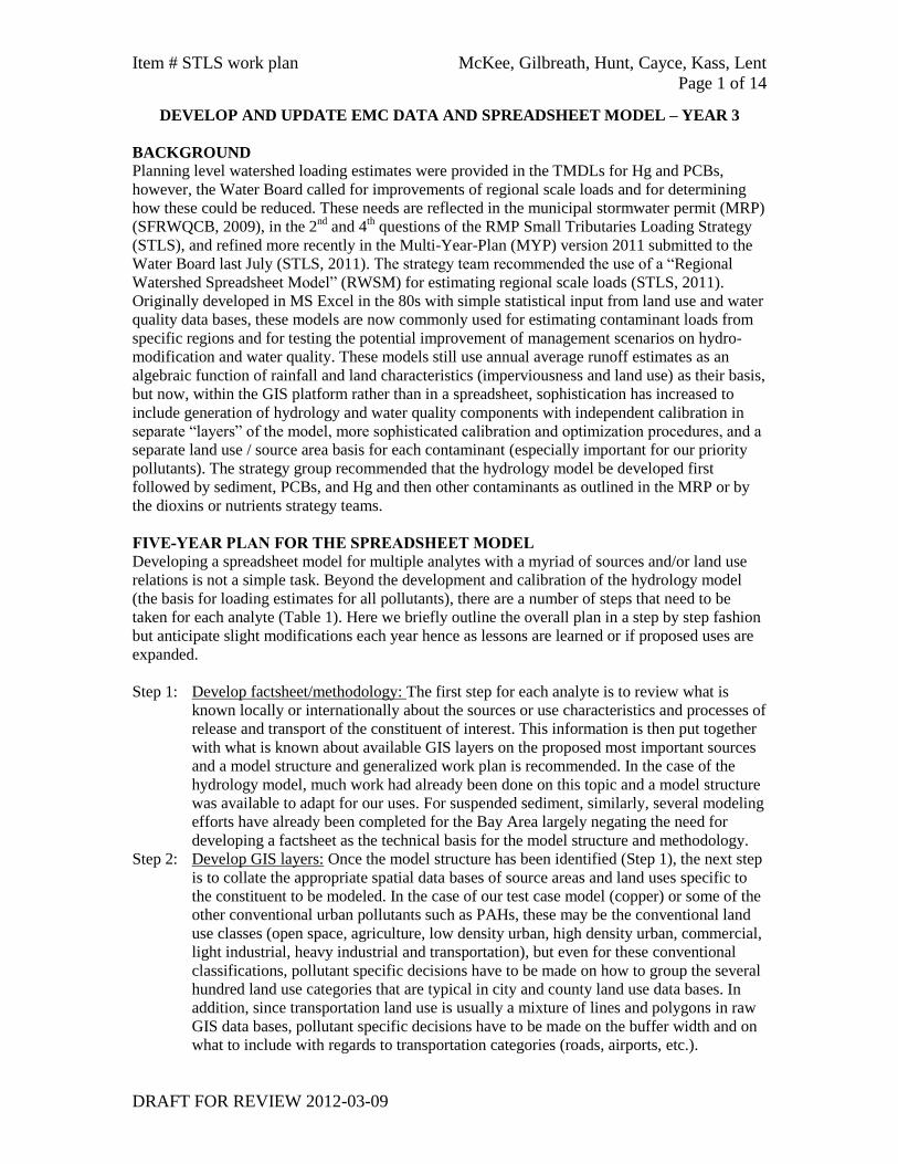
DEVELOP AND UPDATE EMC DATA AND SPREADSHEET MODEL – YEAR 3

BACKGROUND

Planning level watershed loading estimates were provided in the TMDLs for Hg and PCBs,

however, the Water Board called for improvements of regional scale loads and for determining

how these could be reduced. These needs are reflected in the municipal stormwater permit (MRP)

(SFRWQCB, 2009), in the 2nd

and 4th questions of the RMP Small Tributaries Loading Strategy

(STLS), and refined more recently in the Multi-Year-Plan (MYP) version 2011 submitted to the

Water Board last July (STLS, 2011). The strategy team recommended the use of a “Regional

Watershed Spreadsheet Model” (RWSM) for estimating regional scale loads (STLS, 2011).

Originally developed in MS Excel in the 80s with simple statistical input from land use and water

quality data bases, these models are now commonly used for estimating contaminant loads from

specific regions and for testing the potential improvement of management scenarios on hydro-

modification and water quality. These models still use annual average runoff estimates as an

algebraic function of rainfall and land characteristics (imperviousness and land use) as their basis,

but now, within the GIS platform rather than in a spreadsheet, sophistication has increased to

include generation of hydrology and water quality components with independent calibration in

separate “layers” of the model, more sophisticated calibration and optimization procedures, and a

separate land use / source area basis for each contaminant (especially important for our priority

pollutants). The strategy group recommended that the hydrology model be developed first

followed by sediment, PCBs, and Hg and then other contaminants as outlined in the MRP or by

the dioxins or nutrients strategy teams.

FIVE-YEAR PLAN FOR THE SPREADSHEET MODEL

Developing a spreadsheet model for multiple analytes with a myriad of sources and/or land use

relations is not a simple task. Beyond the development and calibration of the hydrology model

(the basis for loading estimates for all pollutants), there are a number of steps that need to be

taken for each analyte (Table 1). Here we briefly outline the overall plan in a step by step fashion

but anticipate slight modifications each year hence as lessons are learned or if proposed uses are

expanded.

Step 1: Develop factsheet/methodology: The first step for each analyte is to review what is

known locally or internationally about the sources or use characteristics and processes of

release and transport of the constituent of interest. This information is then put together

with what is known about available GIS layers on the proposed most important sources

and a model structure and generalized work plan is recommended. In the case of the

hydrology model, much work had already been done on this topic and a model structure

was available to adapt for our uses. For suspended sediment, similarly, several modeling

efforts have already been completed for the Bay Area largely negating the need for

developing a factsheet as the technical basis for the model structure and methodology.

Step 2: Develop GIS layers: Once the model structure has been identified (Step 1), the next step

is to collate the appropriate spatial data bases of source areas and land uses specific to

the constituent to be modeled. In the case of our test case model (copper) or some of the

other conventional urban pollutants such as PAHs, these may be the conventional land

use classes (open space, agriculture, low density urban, high density urban, commercial,

light industrial, heavy industrial and transportation), but even for these conventional

classifications, pollutant specific decisions have to be made on how to group the several

hundred land use categories that are typical in city and county land use data bases. In

addition, since transportation land use is usually a mixture of lines and polygons in raw

GIS data bases, pollutant specific decisions have to be made on the buffer width and on

what to include with regards to transportation categories (roads, airports, etc.).


Page 2 of 14


Table 1. Long term work plan for developing and completing the Regional Watershed Spreadsheet model for each pollutant.

Step Description Flow SS PCBs Hg Cu Se PBDE OC pest Dioxins Nutrients

1 Develop fact sheet / methodology ②

1a Collate local data ③ ① ③ ③ ③ ③ B-2012 B-2012 ③ 2014?

1b

Collate data from review of the world

literature ③ ① ③ ③ ③ ③ B-2012 B-2012 ③ 2014?

1c

Develep source area / land use

categorization conceptual model ③ ① ③ ③ ③ ③ B-2012 B-2012 ③ 2014?

2 Develop GIS layers ③ ① ③ ③

RMP-RWSM-

2012 2013? 2013? 2013? 2014? 2014?

3 Collate input data and calibration data ③ ① ③ ④ ③ ④ ③ 2013? 2013? 2013? 2014? 2014?

4

Run version 1 model and compare with

calibration data ③ ① ③

RMP-RWSM-

2012 2013? 2013? 2013? 2014? 2014?

5 Improve input data and/ or model structure

5a

Back-calculate RCs / EMCs / EFs from local or

world data ④ B-2012

③ 2011

attempt not

sucessful; RMP-

EMC-2012

③ 2011

attempt not

sucessful; RMP-

EMC-2012 RMP-EMC-2012 2013?

5b Improve GIS layers ④ B-2012* RMP-EMC-2012 RMP-EMC-2012 RMP-EMC-2012 2013?

6

Run version 2 model and compare with

calibration data ④ B-2012 RMP-EMC-2012 RMP-EMC-2012 RMP-EMC-2012 2013?

7 Complete FINAL input data set

7a Further refine GIS layers if needed

RMP-RWSM-

2013 -

RMP-EMC-

2012?

RMP-EMC-

2012?

RMP-EMC-

2012? 2013? 2015?

7b Further refine back-calculations if needed - -

RMP-EMC-

2012?

RMP-EMC-

2012?

RMP-EMC-

2012? 2013? 2015?

7c

Perform wet weather field sampling if

needed

RMP-EMC-WY

2013

RMP-EMC-WY

2013

RMP-EMC-WY

2013 TBT

RMP-EMC-WY

2013 TBT

RMP-EMC-WY

2013 TBT

RMP-EMC-WY

2013 TBT

RMP-EMC-WY

2013 TBT 2015?

8

Run version 3 (FINAL) model and complete

calibration / varification

RMP-RWSM-

2014

RMP-RWSM-

2014

RMP-RWSM-

2014

RMP-RWSM-

2014

RMP-RWSM-

2014

RMP-RWSM-

2014

RMP-RWSM-

2014

RMP-RWSM-

2014

RMP-RWSM-

2014 2016?

9 Complete model packaging and user manual RMP-EMC-2012 RMP-EMC-2012 2013? 2013? RMP-EMC-2012 2014? 2014? 2014? 2014? 2016?

①

②

③

④

B

B

*

RMP-RWSM

RMP-EMC

Funding from BASMAA via a contract with ACCWP

Note - the model resolution for sediment will vary from place to place given the need to use measured data where it exists and modeled data where it does not exist

RMP funding ($20k/year) allocated to regional watershed spreadsheet model (RWSM) general development

RMP funding ($80k/year) allocated to EMC development + depending on modeling outcomes perhaps a further $80-100k

Lewicki, M., and McKee, L.J, 2009. Watershed specific and regional scale suspended sediment loads for Bay Area small tributaries. A technical report for the Sources Pathways and Loading Workgroup of the

Regional Monitoring Program for Water Quality: SFEI Contribution #566. San Francisco Estuary Institute, Oakland, CA. 28 pp + Appendices

Ha, S.J., and Stenstrom, M.K., 2008. Predictive Modeling of storm-water runoff quantity and quality for a large urban watershed. Journal of Environmental Engineering 134, 703-711

Lent, M.A. and McKee, L.J., 2011. Development of regional contaminant load estimates for San Francisco Bay Area tributaries based on annual scale rainfall-runoff and volume-concentration models: Year 1

results. A technical report for the Regional Monitoring Program for Water Quality. San Francisco Estuary Institute, Oakland, CA

Lent et al 2012 RWSM y2 documentation memo

Funding from BASMAA via a contract with ACCWP

WG presentation only

PCB/Hg level of effort may not be needed depending on the

level of accuracy needed for the watershed specific and regional

loading estimates

Loads calculation analytes

References


Page 3 of 14


Step 3: Collate input data and calibration data: In the case of the rainfall-runoff model, this

included rainfall data, land use specific runoff coefficients, soils and slope data, and

runoff data for 18+ calibration watersheds. In the case of the sediment model, since we

are modifying an existing model to address known weaknesses, this will only need to

include local geology, classification, and relative erosion rates for each class or

erosional province. Depending on the recommended model structure outlined in the fact

sheet (Step 1) and the availability of spatial data sets (Step 2), for each of the pollutants,

data on land use or source area specific event mean concentrations (EMCs) or soil

concentrations would be collated along with available “bottom of the watershed”

loadings information that has been collected in the past from Bay Area watersheds.

Step 4: Run version 1 of the model: Using the information and data developed in Steps 1, 2, and

3, the model will be run and compared to existing knowledge of loads from watersheds.

This first run will be largely “proof of concept”. Various forms of a sensitivity analysis

can be run on v1 help to determine weaknesses in model structure, input and calibration

data sets so that recommendations can be developed to guide future model versions.

Step 5: Improve model structure and/ or input data: Based on constituent specific

recommendations from step 4, further spatial data base development could occur or

exploration of other sources of coefficients or land use classifications. In addition, in this

task more effort can be put into developing EMC data for model input including EMC

back-calculations upon either water concentration or sediment concentration data or

combinations of both data types either locally available or from elsewhere.

Step 6: Run version 2 of the model: Using the information and data developed in Steps 1, 2, 3,

4, and 5, the model will be run and compared to existing knowledge of loads from

watersheds. This second run will necessarily incorporate a detailed sensitivity analysis

and or/ Monte Carlo techniques to determine weaknesses in model structure, input and

calibration data sets. Very specific recommendations will be developed to prepare for

decisions on further GIS layer development or consolidation, back-calculation

techniques, or a need for specific field data collections to support model improvements.

Step 7: Complete FINAL input data set: Based on constituent specific recommendations and

decisions from step 6, further spatial data base development could occur or exploration

of other sources of coefficients or land use classifications. In addition, more effort can

be put into back-calculation techniques. Pollutant specific EMC data or reconnaissance

bottom of the watershed data in combination with back-calculation techniques may be

collected in the field or specific watersheds may be targeted for bottom of the watershed

loads data to be used for model calibration.

Step 8: Run version 3 (likely FINAL) of the model: Using the information and data developed

this in Steps 1, 2, 3, 4, 5, 6, and 7, the model will be run and compared to existing

knowledge of loads from watersheds. This “FINAL” version will include documentation

of model weaknesses for specific land uses or source areas. In addition, the model

accuracy and precision will be analyzed for each constituent at scales of specific

watersheds, Bay margin segments, and the Bay as a whole.

Step 9: Complete model packaging and user manual: Model packaging and documentation will

be completed to ensure complete transparency between the model development group

(SFEI staff, STLS team) and information users, and that the model results are

repeatable, the model is expandable as appropriate, and that the model is not used for

purposes it is not designed for. Such an open source model will mean that those who are

not the originators of the model can run the model, however an open source model will

require that, from 2012 forward, appropriate model structure and suitable user

documentation is considered at each step of model development.


Page 4 of 14


PROGRESS TO-DATE

During the RMP 2010 calendar year (year 1 of this project), version 1 of the hydrology

component of the regional watershed spreadsheet model (RWSM) was developed. Two base

hydrology model approaches were investigated: one using runoff coefficients based on land use

and the other based on impervious cover. Initial versions of each model were calibrated to local

hydrology data from 18 local watersheds with a wide variety of imperviousness, soil, and slope.

Recommendations were made to address hydrology model weaknesses. The year 1 report also

presented a review of land use and source areas in relation to PCBs, Hg, dioxins, Cu, and Se and

provided recommendations for steps to develop event mean concentration (EMC) data to support

the input side of the model. The report recommended the model structure for each pollutant,

methods to fill data gaps, and priorities (Lent and McKee 2011).

During RMP 2011 calendar year (year 2 of this project), version 2 of the GIS-based model was

developed following Y1 recommendations. In v2, several more calibration watersheds were

added to increase the range of watershed characteristics including %imperviousness character. In

addition, gauge records with incongruent land use / impervious data were removed and land use

categories were refined. For Y3, a focus on the sediment and pollutant models was recommended

(Lent et al., 2012).

In parallel, the BASMAA Monitoring / Pollutants of Concern (POC) Committee has been

discussing and prioritizing work products in relation to the MRP. During 2011, project profiles

were developed for addressing MRP provisions C.8.e.vi (sediment delivery estimate / budget) and

C.14 (PBDEs and OC pesticides). Subsequently, BASMAA has asked SFEI to complete work

outlined in these project profiles. Since all these tasks are components of what is envisioned to be

a single model developed over three years and final report in 2014, this work plan reflects all

recommendations and BASMAA work requests in relation to the RWSM that can be accurately

budgeted at this time. However, we are careful to explicitly describe products and deliverables in

relation to the specific resources allocated by either the RMP or BASMAA.

OBJECTIVES FOR YEAR 3 Step* Task Objective Funding source

2, 3,

4

Cu-2

Cu-3

Cu-4 Cu-9

Complete a copper RWSM as a test case for calibration procedures and to

set reasonable expectations for other contaminants and document outcomes

and recommendations

RMP 2012 RWSM base model

funds

5, 6 SS-5

SS-6 SS-9

Complete an updated version of the sediment RWSM (hybrid), refinement

of the existing model (Lewicki and McKee, 2009) per BASMAA sediment project profile and document outcomes and recommendations

BASMAA funds via ACCWP

contract

2 PCB-2

Hg-2

Complete GIS layer development for PCBs and Hg per recommendations

from the Y1 report (Lent and McKee 2011) including meta data documentation

RMP 2012 EMC development

funds

5 PCB-5

Hg-5

Complete back-calculations of PCB and Hg EMC data using available local

(focus where possible) and literature data per recommendations from the Y1

report (Lent and McKee 2011) and document outcomes and recommendations

RMP 2012 EMC development

funds

6 PCB-6

Hg-6 PCB-9

Hg-9

Complete next versions of the PCB and Hg RWSMs and document

outcomes and recommendations

RMP 2012 AND 2013 RWSM

base funds; RMP 2012 EMC development funds

1 PBDE-1

OCPest-1

Complete contaminant profiles and model workplan recommendations for

PBDE, PBDE, DDT, chlordane, dieldrin per BASMAA project profile

BASMAA funds via ACCWP

contract

0 Mgmt-0 STLS EMC spreadsheet model communication and coordination RMP 2012 EMC development

funds and BASMAA POC

Monitoring Contract

*Refers to steps in Table 1


Page 5 of 14


WORK PLAN FOR YEAR 3

Develop Copper test case Model for RWSM: Copper represents a data rich urban contaminant

that follows classical source, build-up, and wash off processes in relation to

urban land uses in a similar fashion to PAHs and pesticides and parts of the

mercury model process. It therefore represents an ideal test case as a step

toward model development for other contaminants that are of more interest.

There is abundant local land use specific data on copper EMCs (BASMAA,

1995) and abundant bottom of the watershed calibration data (BASMAA,

1995; RMP loading studies, recent BASMAA/ BACWA studies; other SFEI

studies). In addition, there is SPLWG experience and published papers from

SoCal (Stenstrom, Stein and coauthors).

Task Cu-2 Refine GIS data to include transportation land uses.

Deliverable: Transportation GIS data layer

Task Cu-3 Compile EMC data with a focus on local data sets, filling in any data gaps

firstly from SoCal data (compiled by Stein and Stenstrom and coauthors) and

lastly by world data (should not be needed). Budget assumes BASMAA data

base is “model ready”.

Deliverable: Copper EMC Database

Task Cu-4a Complete RWSM v1 and refine based on a sensitivity analysis to each of the

input parameters (land use choices, lumping v splitting land uses, upper and

lower bounds of EMC etc.), Calibration with local bottom-of-the-watershed

data including Guadalupe River, Zone 4 Line A, and possibly Ettie St and

Cerrito Creek and BASMAA 1995 data sets. Comparison of model output to

results of Brake Pad Partnership.

Deliverable: Model calibration and output

Task Cu-4b Complete a short concise report section outlining methods, results and

recommendations briefly (5 pages total). Develop framework for

documentation of hydrology model, document data inventory and metadata for

hydrology model. Example questions to be explored:

Are the data available from 4 watersheds enough for model calibration?

Are the appropriate land uses represented in the calibration watersheds?

Was input data representative of land uses/source areas?

Deliverable: Short technical memo – 5 pages

Task Cu-9 Develop and package a user manual for the Cu model with documentation for

external users of the model including assumptions and recommended uses. Not

budgeted.

Estimated cost: $12,200

Update version of the suspended sediment RWSM: Suspended sediment (SS) is an important

vector for many pollutants. In 2008/09 the RMP completed a detailed analysis

of SS flowing to SF Bay from local tributaries in the 9-counties adjacent to the

Bay (Lewicki and McKee, 2009). During 2011, the first versions of the SS

RWSM was developed using local land use based SSC EMC data (BASMAA,

1995). The results were questionable but informative. The outcomes of the SS

RWSM differed substantially and non-systematically from Lewicki and McKee

(2009) leading us to recommend improving the Lewicki and McKee (2009)

model as the best path. Weakness in the Lewicki and McKee (2009) analysis

included the treatment of urban upland land use categories without regard for


Page 6 of 14


base geology (known to have highly variable erosivity in the Bay Area). SFEI

and many Bay Area consulting firms have completed geomorphic studies that

describe either quantitatively or qualitatively landscape erosion in relation to

land use and geology/soils.

Task SS-5a Complete a status review (of previous Bay Area sediment estimates) and

provide rationale for improvements or modifications to RWSM in a 1-2 page

memo to BASMAA (will become the introduction section in the documented

outcomes)

Deliverable: 1 page memo on recommended RWSM improvements, proposed

tasks budgets and schedules (Appendix A; S1)

Task SS-5b Compile local geology GIS layers, literature and reports, and professional

judgments/ opinions on geological / terrain classes / erosional provinces, and

relative erosion rates. Interpret and complete a classification scheme for Bay

Area urban uplands (values/ ranges/ distributions of sediment-related

coefficients) and route to local professionals for review and input (about 3 local

erosion experts)

Deliverable: Erosion rates classification scheme (Appendix A; S2)

Task SS-6a Migration of Lewicki and McKee (2009) model into compatible format with

RWSM. Complete sediment RWSM v2 testing and calibration, sensitivity

analysis and make any obvious or within budget improvements (Appendix A;

S2)


Task SS-6b Complete model documentation (<10 page memo on methods and results)

including a discussion of uncertainty and data limitations and

recommendations regarding potential improvements and/or data collection, and

relevance to potential use scenarios by Water Board or BASMAA

Deliverable: 10 page technical memo including methods, results and any

recommended phase II improvements (Appendix A; S2)

Task SS-7, 8 PHASE II model improvements and final technical memo for inclusion into

MYP v2013. Scope and budget TBD. (Appendix A; S3)

Task SS-9 Develop and package a user manual for the sediment portion of the model with

documentation for external users of the model including assumptions and

recommended uses. Not budgeted.

Estimated cost: labor $29,250; sub-contracts: $3,000 “data input/ review” from

local erosion experts

GIS layer development for PCBs and Hg: Although Hg and PCB concentrations and loads in

urban landscapes do correlate positively increasing urban land use

density/intensity, this is less likely due to rainfall-wash off processes of

pollutant behavior (like Cu or Zn for instance), but rather due to a greater

density of polluted source areas in relation to land use intensification. A better

model for Hg and PCBs is a combination of land use and source areas emission

factors (Lent and McKee, 2011). Based on the review of local and international

information, PCBs and Hg are likely associated with the manufacture, repair,

testing, storage, and use of electrical transformer and capacitor equipment,

military areas, drum, metals, and auto recycling yards, oil refineries and

petrochemical industrial areas, manufacture of steel or metals, and transport

including rail and shipping. In addition, Hg is also associated with cement

production and cremation. This task will generate the basal land use and source

area geospatial data set to support the Hg and PCB RWSM. There are a range


Page 7 of 14


of challenges including lack of existing published data on some of the proposed

layers and the conversion of line data for form transportation and other land use

/ source area categories in to shape files.

Task PCB&Hg-2aCoordinate with BASMAA by holding 3-3 hour in person meetings to plan

scope of task, level of effort for each land use, and align this effort with other

BASMAA work, prep, and follow-up to meetings. Compile or generate GIS

shape files (polygon or point depending on source type) and associated

metadata in the following order of importance (through a lens of sensible level

of effort):

1. Electrical transformer / capacitor (manufacture/repair/testing/storage/use)

2. Military = Recycling (drum)

3. Cement production

4. Cremation

5. Oil refineries / petrochemicals = Manufacture (steel or metals)

6. Transport (rail) = Transport (ship)

7. Recycling (metals) = Recycling (auto)

Deliverable: GIS data layers (prioritized by STLS)

Task PCB&Hg-2bDevise a QA method, apply it across the layers, and revise / complete meta

data.

Deliverable: Develop QA Methodology and Meta-Data

Task PCB&Hg-2cPrepare a short documentation memo (5 pages) that briefly discusses data

sources, data quality, and potential for improvements. Present results to

SPLWG (1 meeting) and STLS (monthly phone calls during development and

face-to-face).

Deliverable: 5 page technical memo


Back-calculations of PCB and Hg EMC data: During 2011, an unsuccessful attempt was made to

back-calculate EMC data for Hg and PCBs in relation to basic land use

categories using data generated from the 16-watershed reconnaissance loadings

study. Success was limited by too few concentration data in relation to the

number of land uses, a situation that may be rectified through further

reconnaissance. In the meantime, Lent and McKee (2011) recommended the

exploration of EMC back-calculation using a number of other data sets

including land use specific ranges indicated by local data (preferably)

augmented with data from published literature on water and soil concentrations

for water. They proposed a number of methods (which might require further

discussion and refinement) which generally use combinations of either soils or

water data or both to either use matrix algebra or statistical distribution to

determine reasonable ranges in concentration associated with land uses and

source areas. The challenge with methods using soils data is the potential for

underestimation due to a lack of knowledge about concentration factors

between in-situ soil concentrations and those found in stormwater.

Task PCB&Hg-5aCompile local and international data on soils and water concentrations in

relation to land use and source areas for Hg and PCBs (from task 3) ensuring

the resulting data base is well documented

Deliverable: PCB and Mercury EMC database and documentation


Page 8 of 14


Task PCB&Hg-5bResearch various back-calculation methods, including inverse optimization

methods.

Deliverable: Methods for calculating EMCs

Task PCB&Hg-5cProvide regular updates and feedback opportunities to STLS, including

discussion of proposed back-calculation methods.

Deliverable: Project updates at up to 3 STLS meetings

Task PCB&Hg-5dComplete back-calculations, perform sensitivity analysis, and develop error

bars around results (or professional judgment to assign errors or ranges)

Deliverable: EMC back calculation results

Task PCB&Hg-5ePrepare a short (<5 page) summary of methods and results for inclusion in the

model documentation.

Deliverable: 5 page technical memo summarizing methods and results


PCB and Hg Regional Watershed Spreadsheet models (RWSMs): During 2011, the first versions

of the Hg and PCB RWSMs were developed using combinations of SoCal

EMC data (Hg only) and world soils data (Hg and PCBs) combined with local

SSC EMC data (BASMAA, 1995). The Hg load results were consistent with

existing estimates at a regional scale but questionable at the scale of individual

land uses. For PCBs, the loads were 20x higher than expected on a regional

scale and, relatively from one land use to another, in the right order.

Task PCB&Hg-6aReview modeling options (more or less land use / source area classes, hybrid

sediment/water based models) and prepare a short memo (will be a component

of the methods section of the Y3 documentation) that provides the rationale for

each model structure - present model options to STLS.

Deliverable: Short memo of possible modeling options

Task PCB&Hg-6bRefine RWSM to incorporate spatial data created in Task 3 and back

calculations completed in Task 4 into the input data sets. Revise and complete

Hg and PCB RWSM v2 testing and calibration. This will include re-tooling the

model, for speed in use and efficiency in structure, and build a tool interface in

Arc-GIS that can handle both iterative (loop over multiple watersheds) and

single inputs. Evaluate model weaknesses through a sensitivity analysis

(combinations of more and less source area classes and reasonable ranges of

EMCs for each source class, hybrid models) and make any obvious or within

budget improvements. Assumption: The model and documentation will not be

developed for external users. Such documentation may be a prioritized further

step.


Task PCB&Hg-6cComplete model documentation (10 page report section on methods and

results) including a discussion of uncertainty and data limitations and

recommendations regarding potential improvements and/or data collection, and

relevance to potential use scenarios by Water Board or BASMAA.

Deliverable: 10 page technical memo

Task PCB&Hg-9 Develop and package a user manual with documentation for external users of

the PCB and Hg models including assumptions and recommended uses. Not

budgeted.



Page 9 of 14


Contaminant profiles and model workplan recommendations for PBDE, DDT, chlordane, and

dieldrin: During 2010 and 2011, SFEI completed contaminant profiles and

model workplan recommendations for PCBs, Hg, Dioxins, Cu, and Se

(Lent and McKee, 2011). Five components went into developing each

profile: 1. A review of known uses for each substance (Hg, PCBs, Cu,

Dioxins, and Se), 2. a review of regulatory data bases on contaminated

sites/ spills (Hg, PCBs, and Cu), 3. a review of local and world soils

literature (Hg, PCBs, Se), 4. A review of concentrations in stormwater (Hg,

PCBs, Cu, Dioxins, and Se), and 5. A general commentary on presently

known GIS layers in relation to the recommended land use / source area

categories resulting from the first four components. The outcome of this

task will be contaminant profiles and model workplan recommendations

for PBDE, DDT, chlordane, and dieldrin based on a selection of these

steps.

Task PBDE/OCP-1a Review existing contaminant profile structures for Hg, PCBs, Cu, Dioxins,

and Se (Lent and McKee, 2011) and the CMIA reports for PBDEs (Werme

et al., 2007) and OC Pesticides (Connor et al., 2004). Prepare a short (<3

page) memo (note, will become the introduction sections in the

contaminant profiles for each POC) outlining known uses for each

substance (note, we would lump the OC pesticides to reduce the level of

text redundancy), knowledge gaps in previous CMIA reports in relation to

RWSM development, and propose/estimate level of detail for PBDE, DDT,

chlordane, and dieldrin contaminant profiles. Present proposal to STLS for

discussion and decisions.

Deliverable: 3 page technical memo (Appendix A; P1)

Task PBDE/OCP-1b Prepare contaminant profiles and model workplan recommendations for

PBDE, DDT, chlordane, and dieldrin. Base the recommendations on

information gaps or uncertainties for each POC and clarifications from WB

staff regarding potential/desired uses and data quality needs. Document the

outcomes in a short concise technical memo (subsuming the previous effort

for Se (Lent and McKee, 2011)) that addresses the following questions:

1. Is the POC present in urban runoff?

2. Is the POC distributed fairly uniformly in urban areas?

3. Are storm drain systems a generalized source or are there specific

source locations or types?

Present findings and work plan rationale to the STLS for discussion and

decisions on next steps.

Deliverable: Contaminant profiles for PBDEs and OC pesticides

(Appendix A; P2)

Estimated cost (6a-6b): $35,000

Task PBDE/OCP-2a If needed, generate GIS layers to support the RWSM structure for each

POC.

Deliverable: GIS layers for PBDEs and OC pesticides

Estimated cost: Not Budgeted – Year 4 (Appendix A; P3)

Task PBDE/OCP-2b Perform preliminary setup of RWSM to estimate annual loads of PBDE,

DDT, chlordane, dieldrin. Perform preliminary model runs for selected

POCs, depending on available resources and WB interest. Document

findings (<5 pages) with a focus on recommendations that result from

initial model runs appending the previous memo.


Page 10 of 14


Deliverable: 5 page technical memo on model results

Estimated cost: Not Budgeted – Year 4 (Appendix A; P3)

STLS EMC spreadsheet model communication and coordination: In previous years, the RMP

provided separate budget for maintaining communications between STLS

team members. In 2012, budget for communications is assumed to be a

component of the RMP STLS projects.

Task Mgmt-0 Conduct up to 8 STLS phone conferences to update STLS members on

progress, coordinate tasks, solicit feedback and direction, and present

findings. Hold 4 quarterly in-person meetings for discussion and decision

making on WY 2013 additional monitoring activities and review of WY

2012 monitoring activities. Review Multiyear Plan and QAPP draft

documents.


PROJECT BUDGET AND SCHEDULE

The estimated budget (Table 2) is a not-to-exceed amount based on the anticipated time and

materials needed by SFEI to complete the project tasks described in the previous section. The

completion of some of the tasks within the preliminary schedule provided in Table 2 is dependent

upon the timely discussion and agreements by the Water Board and BASMAA.


Page 11 of 14


Table 2. Cost estimates and schedule for completing RWSM components as described in the workplan above.

Old

Task No

New Task No

Description

RMP base model

funds

BASMAA

sediment funds via

ACCWP contract

BASMAA PBDE/

OC pest funds via

ACCWP contract

RMP EMC

development funds

BASMAA POC

Monitoring via

ACCWP

contract

Estimated

Completion

Date

2012

2013

2012

2013

2012

2013

2012

2013

2012

1 Cu-2, 3, 4 Copper test case RWSM $9,700 $2,500

March-July 2012

2 SS-5, 6 Updated version of the

suspended sediment RWSM

$32,250 April-November

2012

3 PCB-2 Hg-2

GIS layer development for PCBs and Hg

$25,850

March-July 2012

4 PCB-5

Hg-5

Back-calculations of PCB and

Hg EMC data

$19,500 July-September

2012

5 PCB-6

Hg-6

PCB and Hg Regional Watershed Spreadsheet models

(RWSMs):

$10,300 $20,000 $12,700

March-July 2013

6

PBDE-1

OCPest-1

Contaminant profiles and

model workplan recommendations for PBDEs,

DDT, chlordane, and dieldrin

$35,000 OC Pest March-

September 2012; PBDE

September-

December 2012

7

Mgmt-0

STLS EMC spreadsheet model

communication and

coordination:

$17,200 $6,800

Ongoing

Total Cost $20,000 $20,000 $32,250 $35,000 $77,750 $6,800

Funds Available $20,000 $20,000 ? ? ? ? $80,000 $80,000 $6,800


Page 12 of 14


REFERENCES

Connor, M., David, J., Leatherbarrow, J., and Werme, C., 2004. Legacy Pesticides in San

Francisco Bay: Conceptual Model/Impairment Assessment. A report prepared for the Clean

Estuary Partnership. San Francisco Estuary Institute, Oakland, CA. 94pp.

Lent, M.A. and McKee, L.J., 2011. Development of regional suspended sediment and pollutant

load estimates for San Francisco Bay Area tributaries based on annual scale rainfall-runoff

and volume-concentration models: Year 1 results. A technical report for the Regional

Monitoring Program for Water Quality. San Francisco Estuary Institute, Oakland, CA.

Lent, M., Gilbreath, A., and McKee, L., 2012. Regional Watershed Spreadsheet Model (RWSM):

Year 2 progress report. A technical progress report prepared for the Regional Monitoring

Program for Water Quality in San Francisco Bay (RMP), Small Tributaries Loading Strategy

(STLS). San Francisco Estuary Institute, Richmond, California.

Lewicki, M., and McKee, L.J., 2009. Watershed specific and regional scale suspended sediment

loads for Bay Area small tributaries. A technical report for the Sources Pathways and

Loading Workgroup of the Regional Monitoring Program for Water Quality: SFEI

Contribution #566. San Francisco Estuary Institute, Oakland, CA. 28 pp + Appendices.

SFRWQCB, 2009. California Regional Water Quality Control Board San Francisco Bay Region

Municipal Regional Stormwater NPDES Permit, Order R2-2009-0074, NPDES Permit No.

CAS612008. Adopted October 14, 2009. 279pp.

http://www.waterboards.ca.gov/sanfranciscobay/board_decisions/adopted_orders/2009/R2-

2009-0074.pdf

STLS, 2011. Small Tributaries Loading Strategy Multi-Year Plan Version 2011. A document

developed collaboratively by the Small Tributaries Loading Strategy Work Group of the

Regional Monitoring Program for Water Quality in the San Francisco Estuary (RMP): Lester

McKee, Alicia Gilbreath, Ben Greenfield, Jennifer Hunt, Michelle Lent, Aroon Melwani

(SFEI), Arleen Feng (ACCWP) and Chris Sommers (EOA/SCVURPPP) for BASMAA, and

Richard Looker and Tom Mumley (SFRWQCB). Submitted to the Water Board, September

2011 to support compliance with the Municipal Regional Stormwater Permit, provision c.8.e.

(http://www.swrcb.ca.gov/rwqcb2/water_issues/programs/stormwater/MRP/2011_AR/BASM

AA/B2_2010-11_MRP_AR.pdf)

Werme, C., Oros, D., Oram, J., McKee, L., and Connor, M., 2007. PBDEs in San Francisco Bay

Conceptual Model/Impairment Assessment. A report prepared for the Clean Estuary

Partnership. SFEI Contribution 429. San Francisco Estuary Institute, Oakland, CA. 59pp.

http://www.waterboards.ca.gov/sanfranciscobay/board_decisions/adopted_orders/2009/R2-2009-0074.pdf

http://www.waterboards.ca.gov/sanfranciscobay/board_decisions/adopted_orders/2009/R2-2009-0074.pdf

http://www.swrcb.ca.gov/rwqcb2/water_issues/programs/stormwater/MRP/2011_AR/BASMAA/B2_2010-11_MRP_AR.pdf

http://www.swrcb.ca.gov/rwqcb2/water_issues/programs/stormwater/MRP/2011_AR/BASMAA/B2_2010-11_MRP_AR.pdf


Page 13 of 14


Appendix A

Sediment and MRP C.14 Contaminants Regional Loads Estimation: Revised August 2012

Multi-year Deliverables List

The table below lists the key SFEI deliverables for Sediment Estimate (S prefix) and Permit-

specific Contaminants (P prefix) regional projects to be implemented through ACCWP Action

Plans starting with C14-1-12. The right hand column describes, for planning purposes, assumed

interim steps or products that will inform or be incorporated into each deliverable. There can be

some flexibility in the alignment of these interim steps with key deliverable dates, e.g. degree of

finalization of individual contaminant profiles for Deliverable P-2.

The ACCWP Action Plans will be based on the S and P workplans which should be integrated

with each other and also with updates to the STLS and Regional Watershed Spreadsheet Model

Multi-year Plans. It is assumed that SPLWG review or comment will be solicited and incorporated

at each stage, especially for sediment deliverables. The Sediment and Permit-specific

Contaminants interim schedules should be coordinated with other scheduling considerations for

SPLWG but preference is for early review or feedback on presentation of interim results/products

rather than commenting on draft final deliverables.

Item Target Deliverable Interim steps or products

S-1 Final draft

for MPC

2/9/12

Final 3/1/12

Workplan, detailed through

2012 and draft through 2013

(add text, tables to STLS MYP

V2012A, or else reference as

stand-alone appendix to STLS

MYP and BASMAA

Monitoring Status Report)

Status review (vs. previous Bay Area

estimates)

Rationale for improvements or

modifications to RWSM

Proposed tasks, budget and schedule

through 2013

S-2 Final draft

for MPC

11/2/12

Status memo for update to

STLS Work Group Propose modifications to RWSM

Develop values/ranges/distributions of

sediment-related coefficients

Clarification from WB staff re

potential/desired uses for estimates,

e.g. data quality needs, for which other

contaminants is sediment likely to be

used as a surrogate?

S-3 Final draft

for MPC

1/2/

Final

1/25/13

Summary memo on initial

sediment estimates, with

appended “sediment profile”

(incorporate as stand-alone

appendix in STLS MYP

V2013, and in BASMAA

Urban Creeks Monitoring

Report)

Model testing, calibration

Coordination with RMP-funded POC

model testing (i.e. PCBs)

Model refinements, testing, (limited?)

sensitivity analysis

discussion of uncertainty and data

limitations

recommendations re potential

improvements and/or data collection,

and relevance to potential use

scenarios by WB or BASMAA


Page 14 of 14


Appendix A continued

Sediment and MRP C.14 Contaminants Regional Loads Estimation: Revised August 2012

Multi-year Deliverables List

P-1 Final draft

for MPC

2/9/12

Final 3/1/12

Workplan, detailed through

2012 and draft through 2013

(add text, tables to STLS MYP

V2012A, or else reference as

stand-alone appendix to STLS

MYP and BASMAA Monitoring

Status Report)

Reference previous CMIA reports by

CEP, other potential info sources

Reference RMP-funded RWSM

contaminant profile & modeling

workplan for Se

Propose/estimate level of detail to be

used in contaminant profiles for

PBDE, DDT, chlordane, dieldrin

P-2 Final draft

for MPC

11/20/12

Final

1/25/13

Memo on characterization of

PBDEs, legacy pesticides and

Se addressing MRP questions:

Is it present in urban runoff?

Is it distributed fairly

uniformly in urban areas?

Are storm drain systems a

generalized source or are there

specific source locations or

types?

Working, draft or final draft

Contaminant profiles for PBDE,

DDT, chlordane, dieldrin (BASMAA

funded) and Se (RMP funded)

Evaluate information gaps or

uncertainties for each POC

Clarification from WB staff re

potential/desired uses and DQ needs

for estimating loads of each POC

P-3 Final draft

for MPC

5/31/13

Final

7/26/13

Report with information

required to compute regional

loads to SF Bay from urban

runoff conveyance systems

Contaminant profiles for PBDE,

DDT, chlordane, dieldrin (BASMAA

funded) and Se (RMP funded)

Preliminary setup of RWSM to

estimate annual loads of PBDE,

DDT, chlordane, dieldrin

(Preliminary model runs for selected

POCs may be added, depending on

available resources and WB interest)

P-4 Workplan

Oct 2012

Final draft

May 2013

Review and comment on report

identifying control measures

and/or management practices

(workplan, reports by others)

SAN FRANCISCO ESTUARY INST ITUTE CONTRIBUTION

NO. 667

MAY2012

4911 Central Avenue, Richmond, CA 94804

p: 510-746-7334 (SFEI), f: 510-746-7300,

www.sfei.org

Development of Regional Suspended Sediment and Pollutant Load Estimates for San Francisco Bay Area Tributaries using the Regional Watershed Spreadsheet Model (RWSM): Year 2 Progress Report

Prepared by

Michelle A. Lent

Alicia N. Gilbreath

Lester J. McKee

San Francisco Estuary Institute

For

The Regional Monitoring Program for Water Quality

in San Francisco Bay (RMP)

Small Tributaries Loading Strategy (STLS)

RWSM – Year 2 progress report Page 1 of 17

Acknowledgements

We were glad for the support and guidance of the Sources, Pathways and Loadings Workgroup of the Regional Monitoring Program for Water Quality in San Francisco Bay. In addition, the detailed work

plans that lead to this progress report was developed through the Small Tributaries Loading Strategy (STLS) during a series of meetings that began in 2008 and continue today. Local members on the STLS are Arleen Feng, Chris Sommers, and Jamison Crosby (for BASMAA) and Richard Looker, Jan O’Hara, and

Tom Mumley (for the Water Board). The external reviewer members who were part of the STLS were Eric Stein (SCCWRP) and Mike Stenstrom (UCLA). We are particularly indebted to their helpful comments during product concept development. We received helpful comments from Eric Stein, Mike Stenstrom

and Barbara Mahler during and through email and phone calls after work group meetings. We are indebted to workgroup members who provided review comments during the product development phase and early draft materials for this report including Arleen Feng, Chris Sommers and Richard Looker.

Ben Greenfield, Greg Shellenbarger, Michael Stenstrom, and Peter Mangarella provided helpful written reviews on the draft report that we incorporated to improve this final progress report. This project was funded as a special study by the Regional Monitoring Program for Water Quality in San Francisco Bay.

This progress report can be cited as:

Lent, M., Gilbreath, A., and McKee, L., 2012. Development of regional suspended sediment and pollutant

load estimates for San Francisco Bay Area tributaries using the regional watershed spreadsheet model (RWSM): Year 2 progress report. A technical progress report prepared for the Regional Monitoring Program for Water Quality in San Francisco Bay (RMP), Small Tributaries Loading Strategy (STLS).

Contribution No. 667. San Francisco Estuary Institute, Richmond, California.


Table of Contents

Acknowledgements...................................................................................................................... 1

Introduction, context and objectives ............................................................................................ 3

Improved calibration data set ...................................................................................................... 4

Refined land use input data.......................................................................................................... 9

Conclusion ................................................................................................................................. 10

References ................................................................................................................................. 13

Appendix -‐ Revised land use classification for runoff coefficients. .............................................. 15


Introduction, context and objectives

The RMP is providing direct support for answering specific Management Questions through multi-‐year Strategies consisting of coordinated activities centered on particular pollutants of concern (POCs) or

processes. The Small Tributaries Loading Strategy (STLS, SFEI, 2009) presented an initial outline of the general strategy and activities to address four key Management Questions:

1. Which Bay tributaries (including stormwater conveyances) contribute most to Bay impairment from POCs;

2. What are the annual loads or concentrations of POCs from tributaries to the Bay; 3. What are the decadal-‐scale loading or concentration trends of POCs from small tributaries to the

Bay; and,

4. What are the projected impacts of management actions (including control measures) on tributaries and where should these management actions be implemented to have the greatest beneficial impact.

Since then, a Multi-‐Year-‐Plan (MYP) (STLS, 2011) has been written that provides a more comprehensive description of activities that will be included in the STLS over the next 5-‐10 years in order to provide

information in compliance with the municipal regional stormwater permit (MRP; Water Board 2009). The MYP provides detailed rationale for the methods and locations of proposed activities, including loads monitoring of local tributaries. The MYP, which will be updated at least once a year to reflect

evolving information, recommended the development of the Regional Watershed Spreadsheet Model (RWSM) as a tool for estimating regional loads. Point-‐source loads, though covered in TMDLs or other potential regulatory activities, are not included in this model.

The first phase of the project (Year 1) served to develop a GIS-‐based regional rainfall-‐runoff model,

calibrate the hydrology, collate land use / source specific concentration data for pollutants of interest, and perform initial forays into sediment and pollutant models (Lent and McKee, 2011). The RWSM Year 1 report concluded that there were concerns with the hydrologic calibration data set and with the

underlying land use data set, and that the immediate next steps should be to refine hydrology model by:

• Adding several calibration watersheds to ensure watershed characteristics spanned a wider range of imperviousness including more of the higher %IC character

• Removing any gage records incongruent with land use / impervious data

• Refining land use categories and re-‐calibrating model This write-‐up serves to document these model refinements performed during year 2 of the RWSM

development. At the end of year 2, no further hydrologic model refinement was recommended as a priority in year 3; focus should now shift to the sediment and contaminant models. However, development and calibration of a selection of water quality models in year 3 may highlight weaknesses

in the hydrological model that may need to be addressed in year 4 in concert with other priorities identified at that time.


Improved calibration data set

The original calibration data set used in the RWSM Y1 model (Lent and McKee, 2011) lacked representation at the high end of the imperviousness range. This was was problematic because highly impervious areas contribute disproportionately to runoff and because San Francisco Bay is ringed by

highly developed flatlands. Only one of the original watersheds had greater than 50% impervious surface (Figure 1). To better represent the range of development conditions present in the Bay Area, we added three high imperviousness watersheds to the calibration data set: Ettie Street Pump Station (79%

impervious), Victor-‐Nelo Pump Station (88%) and Laurelwood Pump Station (74%) (Figure 1, right side). In keeping with Bay Area development patterns, all of the high imperviousness watersheds added were in the highly developed lowlands. Additionally, the sites added were all pump stations due to the lack of

flow monitoring in highly urban watersheds. The added advantage of including these watersheds is they might also include some of the source areas proposed for structuring the PCB and Hg model components.

The data sets for all of the pump stations were derived from pump run logs, which were converted to

estimated flow using the maximum pump capacity for each station. This assumption of instantaneous pump “run-‐up” and maximum rated capacity introduces errors, but they are likely small relative to the overall magnitude of flow volume passed by the pumps. To check if the pump data logs seemed

reasonable, we plotted monthly rainfall versus estimated flow volume using the 5 months of data available for each station (Figure 2). The pump data showed a good correlation with rainfall for the two South Bay pump stations. Based on 41 months of data, Ettie Street pump station records exhibited a

strong relationship with rainfall as well (R2 = 0.98, data not shown).

Figure 1 -‐ Percent imperviousness in the original (Left) and updated (Right) calibration watershed data

set. The left panel shows the RWSM Y1 calibration data with only one watershed with >50%

impervious surface.


Figure 2 -‐ Correlation between flow obtained by conversion of the pump data logs (using assumptions

about pump capacity) and rainfall.

Aside from the lack of representation at the high end of the imperviousness range in the original calibration data set, we were also concerned about potential incongruence between disparate non stationary data that represents differing time periods. Given that we were using a land use and

impervious surface data set from the 1990-‐2000s to estimate runoff coefficients, some of the older gage records potentially were not representative of more recent hydrological behavior in some of the calibration watersheds, especially if significant development had occurred in the watershed between

the start of the gage data record and the 1990s. We checked the older (pre-‐1990s) gage records for watersheds with ≥5% built impervious surface for changes in runoff behavior over time. In some watersheds, a distinct development signal was shown by the increase in runoff coefficient by decade; a

prime example is Colma Creek, which underwent massive development over the period of flow monitoring (Figure 3). As a result of this analysis, we removed earlier portions of several gage records (Colma Creek, Matadero Creek, and Walnut Creek). Additionally we completely removed two records

which ended too early to properly evaluate hydrologic changes relative to more recent conditions: Arroyo Corte Madera (1966-‐1986) and Wildcat Creek at Richmond (1965-‐1975).

Watersheds in our calibration data set span the entire spatial geography of the Bay Area and incorporate watersheds that represent a wide range of imperviousness (Table 1). A flow record actually

exists for Sunnyvale East Channel, but unfortunately it is of poor quality (pers. comm., Ken Stumpf, SCVWD), which was apparent when the record was regressed against rainfall (R2 = 0.58). Upon further analysis, based on regression with rainfall data, data quality was found to be good before 2001. This

subset of data was initially used in the calibration but Sunnyvale Creek was found to be the worst performer in the model amongst all the calibration watersheds again casting dispersion on data quality. We decided to reject incorporating it at this time but may include it in the future once data generated

by SFEI monitoring efforts can be used to verify quality. Our basic check of data quality revealed very


Figure 3 -‐ Colma Creek rainfall-‐runoff relationship changing over time.

Table 1 -‐ Updated calibration watershed set.

Watershed County Agency / Gage ID Gage Record Used % Built

Imp. c.2000 Canoas Creek Santa Clara SCVWD 1485 1995-‐2007 46 Castro Valley Creek Alameda USGS 11181008 1972-‐2009 46 Colma Creek San Mateo USGS 11162720 (REVISED) 1981-‐1994 38 Dry Creek Napa USGS 11458500 1952-‐1966 0.1 Matadero Creek Santa Clara USGS 11166000 (REVISED) 1981-‐2009 17 Novato Creek Marin USGS 11459500 1947-‐2009 3 Pinole Creek Contra Costa USGS 11182100 1940-‐1977 0.3 Corte Madera Creek Marin USGS 11460000 1952-‐1993 5 Ross Creek Santa Clara SCVWD 2058 1995-‐2007 36 San Ramon Creek Contra Costa USGS 11182500 1953-‐2009 3 San Tomas Creek Santa Clara SCVWD 2050 1973-‐2009 30 Sonoma Creek Sonoma USGS 11458500 1956-‐1981; 2002-‐2009 2 Upper Napa River Napa USGS 11456000 1940-‐1995; 2001-‐2009 2 Walnut Creek Contra Costa USGS 11183600 (REVISED) 1981-‐-‐1992 13 Wildcat Creek -‐ Vale Contra Costa USGS 11181390 1976-‐1995 4 Zone 4 Line A Channel Alameda SFEI (no ID) 2007-‐2010 71 San Leandro Creek Alameda SFEI (no ID) To be monitored WY2012 38 Sunnyvale East Channel Santa Clara SFEI (no ID) To be monitored WY2012 59 Victor-‐Nelo Pump Station Santa Clara City of Santa Clara 2009-‐2010 88 Laurelwood Pump Station Santa Clara City of Santa Clara 2009-‐2010 74 Ettie St. Pump Station Alameda ACFCD 2005-‐2008 79

strong relationships between a local representative rainfall data set and the annual runoff ranging

between r2=0.78 to r2=0.98 (Table 2).

The model was rerun using the reevaluated watershed calibration data sets that included dropping some watersheds and picking up others (Table 3). Unfortunately, the model performance worsened with the updated calibration data set. The two worst performers in the revised data set were the South Bay


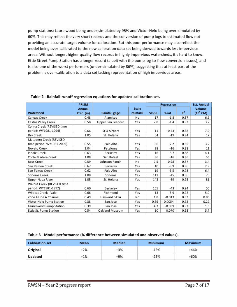
pump stations: Laurelwood being under-‐simulated by 95% and Victor-‐Nelo being over-‐simulated by 60%. This may reflect the very short records and the conversion of pump logs to estimated flow not

providing an accurate target volume for calibration. But this poor performance may also reflect the model being over-‐calibrated to the new calibration data set being skewed towards less impervious areas. Without longer, higher quality flow records in highly impervious watersheds, it’s hard to know.

Ettie Street Pump Station has a longer record (albeit with the pump log-‐to-‐flow conversion issues), and is also one of the worst performers (under-‐simulated by 86%), suggesting that at least part of the problem is over-‐calibration to a data set lacking representation of high impervious areas.

Table 2 -‐ Rainfall-‐runoff regression equations for updated calibration set.

Regression

Watershed

PRISM Annual Prec. (m) Rainfall gage

Scale rainfall? Slope Y-‐int. R2

Est. Annual Volume (106 CM)

Canoas Creek 0.48 Alamitos No 17 -‐1.8 0.87 6.6 Castro Valley Creek 0.58 Upper San Leandro Yes 7.8 -‐1.4 0.93 3.2 Colma Creek (REVISED time period: WY1981-‐1994) 0.66 SFO Airport Yes 11 +0.73 0.88 7.9 Dry Creek 1.05 St. Helena Yes 34 -‐19 0.94 17 Matadero Creek (REVISED time period: WY1981-‐2009) 0.55 Palo Alto Yes 9.6 -‐2.2 0.85 3.2 Novato Creek 1.04 Petaluma Yes 28 -‐16 0.88 11 Pinole Creek 0.63 Berkeley Yes 16 -‐5.7 0.88 4.1 Corte Madera Creek 1.08 San Rafael Yes 36 -‐16 0.86 55 Ross Creek 0.59 Johnson Ranch No 7.5 -‐0.98 0.87 3.4 San Ramon Creek 0.67 Berkeley Yes 10 -‐3.9 0.86 2.9 San Tomas Creek 0.62 Palo Alto Yes 19 -‐5.5 0.78 6.4 Sonoma Creek 1.08 Sonoma Yes 111 -‐45 0.86 75 Upper Napa River 1.05 St. Helena Yes 143 -‐69 0.95 81 Walnut Creek (REVISED time period: WY1981-‐1992) 0.60 Berkeley Yes 155 -‐43 0.94 50 Wildcat Creek -‐ Vale 0.66 Richmond Yes 13 -‐3.9 0.92 5.0 Zone 4 Line A Channel 0.49 Hayward 541A No 1.8 -‐0.013 0.93 0.86 Victor-‐Nelo Pump Station 0.38 San Jose Yes 0.59 -‐0.0054 0.92 0.22 Laurelwood Pump Station 0.39 San Jose Yes 4.3 -‐0.039 0.92 1.6 Ettie St. Pump Station 0.54 Oakland Museum Yes 10 0.070 0.98 5.7

Table 3 -‐ Model performance (% difference between simulated and observed values).

Calibration set Mean Median Minimum Maximum

Original +2% +3% -‐42% +46%

Updated +1% +9% -‐95% +60%


Another possibility is the assumption of linearity in the relationship between imperviousness and the resulting runoff coefficient. For example, in the LA region (even more arid than the Bay Area), a

curvilinear function has been applied (Figure 4) (Peter Mangarella, GeoSyntec Consultants, Oakland, personal communication, February 2012). In addition another problem with runoff coefficient modeling method is that contribution from both impervious and pervious areas can vary depending on storm size

and season (soil moisture content and evapotranspiration). This has been discussed extensively in science literature and was documented by M.I Budyko in 1974. The “Budyko curve”, as it came to be referred to, describes the relationship between climate, evapotranspiration and runoff (Donohue et al.,

2006; Gerrits et al., 2009). The explicit outcome of the curve is that watersheds of differing rainfall and heat should have differing inter-‐annual rainfall -‐runoff functions. Thus, the centrality of the medium or mean relative to the runoff extremes in reaction to rainfall extremes will be a function of aridity. This is

presently not incorporated into the year 2 version of the RWSM but could be in future versions. This appears consistent with experience in Wisconsin, where runoff coefficients have been defined as a function of both land use and percent connected imperviousness and rainfall depth (Roger Bannerman,

personal communication, December 2011).

Figure 4. Runoff coefficients as a function of imperviousness. Source: Peter Mangarella, GeoSyntec Consultants, Oakland.


Refined land use input data

During development of the base hydrology model, we noticed that the land use layer (ABAG 2000) contained discrepancies related to transportation land use. Specifically, for Alameda and Santa Clara counties, local roads were not broken out into their own category (Figure 5) as they had been for the

other Bay Area counties. Upon close inspection, it was noted that the land use resolution varied dramatically between counties (Figure 6). These discrepancies were corrected in the updated land use layer (ABAG 2005). Accordingly the model was re-‐developed using the improved ABAG 2005 land use

data set.

Figure 5 -‐ Discrepancies in ABAG 2000 data set for transportation land use.

Figure 6 – ABAG 2000 versus ABAG 2005 (zoomed to border of Contra Costa and Alameda Counties).


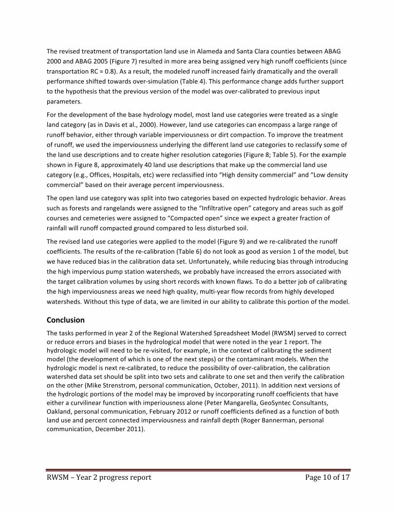
The revised treatment of transportation land use in Alameda and Santa Clara counties between ABAG 2000 and ABAG 2005 (Figure 7) resulted in more area being assigned very high runoff coefficients (since

transportation RC = 0.8). As a result, the modeled runoff increased fairly dramatically and the overall performance shifted towards over-‐simulation (Table 4). This performance change adds further support to the hypothesis that the previous version of the model was over-‐calibrated to previous input

parameters.

For the development of the base hydrology model, most land use categories were treated as a single land category (as in Davis et al., 2000). However, land use categories can encompass a large range of

runoff behavior, either through variable imperviousness or dirt compaction. To improve the treatment of runoff, we used the imperviousness underlying the different land use categories to reclassify some of the land use descriptions and to create higher resolution categories (Figure 8; Table 5). For the example

shown in Figure 8, approximately 40 land use descriptions that make up the commercial land use category (e.g., Offices, Hospitals, etc) were reclassified into “High density commercial” and “Low density commercial” based on their average percent imperviousness.

The open land use category was split into two categories based on expected hydrologic behavior. Areas

such as forests and rangelands were assigned to the “Infiltrative open” category and areas such as golf courses and cemeteries were assigned to “Compacted open” since we expect a greater fraction of rainfall will runoff compacted ground compared to less disturbed soil.

The revised land use categories were applied to the model (Figure 9) and we re-‐calibrated the runoff coefficients. The results of the re-‐calibration (Table 6) do not look as good as version 1 of the model, but we have reduced bias in the calibration data set. Unfortunately, while reducing bias through introducing

the high impervious pump station watersheds, we probably have increased the errors associated with the target calibration volumes by using short records with known flaws. To do a better job of calibrating the high imperviousness areas we need high quality, multi-‐year flow records from highly developed

watersheds. Without this type of data, we are limited in our ability to calibrate this portion of the model.

Conclusion

The tasks performed in year 2 of the Regional Watershed Spreadsheet Model (RWSM) served to correct or reduce errors and biases in the hydrological model that were noted in the year 1 report. The hydrologic model will need to be re-‐visited, for example, in the context of calibrating the sediment model (the development of which is one of the next steps) or the contaminant models. When the hydrologic model is next re-‐calibrated, to reduce the possibility of over-‐calibration, the calibration watershed data set should be split into two sets and calibrate to one set and then verify the calibration on the other (Mike Strenstrom, personal communication, October, 2011). In addition next versions of the hydrologic portions of the model may be improved by incorporating runoff coefficients that have either a curvilinear function with imperiousness alone (Peter Mangarella, GeoSyntec Consultants, Oakland, personal communication, February 2012 or runoff coefficients defined as a function of both land use and percent connected imperviousness and rainfall depth (Roger Bannerman, personal communication, December 2011).


Figure 7 -‐ Changes in land use classification from ABAG 2000 to ABAG 2005 for calibration watersheds.

Table 4 -‐ Model performance for different land use data sets (using updated watershed set).

Land use data set Mean Median Minimum Maximum

ABAG 2000 +1% +9% -‐95% +60%

ABAG 2005 +13% +17% -‐78% +79%


Figure 8 – An example of using imperviousness to reclassify land use descriptions into categories that more accurately group runoff behavior

Table 5 – Revised higher resolution categories for assignment of runoff coefficients. Note the full

listing of land use descriptions with assigned categories and average percent impervious is presented in the Appendix.

Original Categories Revised Categories Agriculture Agriculture

Open Open

Open – compacted

Residential – rural Residential – low Residential – med

Residential

Residential – high Commercial – low Commercial Commercial – high

Industrial Industrial Transportation Transportation

Water Water Water – runoff


Figure 9 -‐ Distribution of revised land use categories in calibration watershed set.

Table 6 -‐ Model performance.

Model Mean Median Minimum Maximum

Uncalibrated ABAG 2005 +13% +17% -‐78% +79%

Calibrated ABAG 2005 (rev. cat.) +1% +3% -‐75% +70%

References

ABAG, 2000. Description of land use classifications categories. Association of Bay Area Governments

(ABAG), Oakland, CA.

ABAG, 2005. 2006. Existing Land Use in 2005: Data for Bay Area Counties. Oakland, California USA. DVD.

Davis, J.A., L. McKee, J. Leatherbarrow, and T. Daum. 2000. Contaminant Loads from Stormwater to Coastal Waters in the San Francisco Bay Region: Comparison to Other Pathways and Recommended Approach for Future Evaluation. San Francisco Estuary Institute, Richmond, CA.

Donohue, R. J., M. L. Roderick, and T. R. McVicar (2007), On the importance of including vegetation

dynamics in Budyko’s hydrological model, Hydrol. Earth Syst. Sci., 11, 983– 995.

Gerrits, A. M. J., H. H. G. Savenije, E. J. M. Veling, and L. Pfister. Analytical derivation of the Budyko curve based on rainfall characteristics and a simple evaporation model. Water Resources Research 45, W04403, 15 pp.

Lent, M.A. and McKee, L.J., 2011. Development of regional suspended sediment and pollutant load

estimates for San Francisco Bay Area tributaries using the regional watershed spreadsheet model


(RWSM): Year 1 progress report. A technical report for the Regional Monitoring Program for Water Quality, Small Tributaries Loading Strategy (STLS). Contribution No. 666. San Francisco Estuary

Institute, Richmond, CA.

SFEI, 2009. RMP Small Tributaries Loading Strategy. A report prepared by the strategy team (L McKee, A Feng, C Sommers, R Looker) for the Regional Monitoring Program for Water Quality. SFEI Contribution #585. San Francisco Estuary Institute, Oakland, CA. xxpp.

STLS, 2011. Small Tributaries Loading Strategy Multi-‐Year Plan Version 2011. A document developed

collaboratively by the Small Tributaries Loading Strategy Work Group of the Regional Monitoring Program for Water Quality in the San Francisco Estuary (RMP): Lester McKee, Alicia Gilbreath, Ben Greenfield, Jennifer Hunt, Michelle Lent, Aroon Melwani (SFEI), Arleen Feng (ACCWP) and Chris

Sommers (EOA/SCVURPPP) for BASMAA, and Richard Looker and Tom Mumley (SFRWQCB). Submitted to the Water Board, September 2011 to support compliance with the Municipal Regional Stormwater Permit, provision C.8.e.

(http://www.swrcb.ca.gov/rwqcb2/water_issues/programs/stormwater/MRP/2011_AR/BASMAA/B2_2010-‐11_MRP_AR.pdf )

Water Board, 2009. California Regional Water Quality Control Board San Francisco Bay Region Municipal Regional Stormwater NPDES Permit, Order R2-‐2009-‐0074, NPDES Permit No. CAS612008. Adopted

October 14, 2009. 279pp. http://www.waterboards.ca.gov/sanfranciscobay/board_decisions/adopted_orders/2009/R2-‐2009-‐0074.pdf


Appendix -‐ Revised land use classification for runoff coefficients.

Land Use Description Original Reclassification New Reclassification Mean % Imp. Cropland & Pasture Agriculture Agriculture 1 Cropland Agriculture Agriculture 1 Confined Feeding (Including Feed Lots) Agriculture Agriculture 3 Small Grains Agriculture Agriculture 3 Pasture Agriculture Agriculture 4 Orchards, Groves, Vineyards, And Nurseries Agriculture Agriculture 6 Row Crops Agriculture Agriculture 6 Vineyards And Kiwi Fruit Agriculture Agriculture 11 Farmsteads And Agricultural Buildings Agriculture Agriculture 13 Orchards Or Groves Agriculture Agriculture 13 Military Installations Commercial Commercial -‐ low 13 Military Hospital Commercial Commercial -‐ low 14 Transitional Or Mixed Use Of Land Areas Commercial Commercial -‐ low 17 Medical Clinics Commercial Commercial -‐ low 20 Colleges & Universities Commercial Commercial -‐ low 24 Greenhouses And Floriculture Agriculture Commercial -‐ low 29 Stadiums Commercial Commercial -‐ low 32 Local Gov't Jails And Rehab Centers Commercial Commercial -‐ low 33 Extensive Recreation Open Commercial -‐ low 33 State Prisons Commercial Commercial -‐ low 35 Medical Long-‐Term Care Facilities Commercial Commercial -‐ low 36 Transitional Areas Open Commercial -‐ low 37 City Halls & Co., State, Fed. Govt. Facilities Commercial Commercial -‐ low 38 Education Commercial Commercial -‐ low 38 Elementary & Secondary Schools Commercial Commercial -‐ low 39 Mixed Commercial & Industrial Complexes Commercial Commercial -‐ low 41 Other Transitional Open Commercial -‐ low 42 Commercial Or Services Vacant Open Commercial -‐ low 44 Museums And Libraries Commercial Commercial -‐ low 44 Commercial Commercial Commercial -‐ low 45 Closed Military Facilities Commercial Commercial -‐ low 45 Communications Facilities Commercial Commercial -‐ low 46 Local Government And Other Public Facilities Commercial Commercial -‐ low 47 Churches, Synagogues, And Mosques Commercial Commercial -‐ low 47 Community Hospitals Commercial Commercial -‐ high 52 Convention Centers Commercial Commercial -‐ high 54 Daycare Facilities Commercial Commercial -‐ high 56 Hospitals, Rehab, Health, & State Prisons Commercial Commercial -‐ high 61 Hotels And Motels Commercial Commercial -‐ high 62 Stadium Commercial Commercial -‐ high 62 Research Centers Commercial Commercial -‐ high 64 Offices Commercial Commercial -‐ high 64 Hosptals -‐ Designated Trauma Centers Commercial Commercial -‐ high 64 Fire Station Commercial Commercial -‐ high 65 Mixed Use In Buildings Commercial Commercial -‐ high 67 Retail And Wholesale Commercial Commercial -‐ high 68 Police Station Commercial Commercial -‐ high 71 Warehousing Commercial Commercial -‐ high 79 Out-‐Patient Surgery Centers Commercial Commercial -‐ high 85 Strip Mines & Quarries, Commercial Opera Industrial Industrial 23 Water Storage (Covered) Industrial Industrial 26


Land Use Description Original Reclassification New Reclassification Mean % Imp. Food Processing Industrial Industrial 26 Municipal Water Supply Facilities Industrial Industrial 32 Wastewater Treatment Plant Industrial Industrial 34 Water Treatment (Filtration) Plant Industrial Industrial 35 Earth Works Not Part Of Commercial Extra Open Industrial 36 Industrial Vacant Open Industrial 39 Electric, Other Industrial Industrial 40 Electric Substation Industrial Industrial 47 Heavy Industrial Industrial Industrial 52 Wastewater Storage Industrial Industrial 54 Light Industrial Industrial Industrial 55 Wastewater Pumping Station Industrial Industrial 57 Industrial Industrial Industrial 69 Electric Power Plant Industrial Industrial 72 Media Broadcast Towers And Facilities Industrial Industrial 84 State Psychiatric Facilities Commercial Open -‐ Compacted 0 Camps And Campgrounds Open Open -‐ Compacted 1 State Mental Health And Devel. Disabled Commercial Open -‐ Compacted 2 Military Open Areas Open Open -‐ Compacted 4 Golf Courses Open Open -‐ Compacted 7 Military -‐ General Use Commercial Open -‐ Compacted 9 Urban Open Space -‐ Slated For Redevelopment Open Open -‐ Compacted 10 Racetracks Open Open -‐ Compacted 11 Bare Exposed Rock Open Open -‐ Compacted 14 Cemeteries Open Open -‐ Compacted 14 Residential Vacant Open Open -‐ Compacted 14 Urban Parks Open Open -‐ Compacted 17 Commonly Owned Residential, No Du Residential Open -‐ Compacted 18 Other Urban And Built-‐Up Land Open Open -‐ Compacted 20 Sanitary Landfills Open Open -‐ Compacted 23 Commercial Intensive Outdoor Recreation Open Open -‐ Compacted 24 Urban Vacant Undeveloped Land Open Open -‐ Compacted 25 Nonforested Wetlands Open Open 2 Mixed Forest -‐ Protected As Park Open Open 3 Evergreen Forest -‐ Protected As Park Open Open 3 Salt Evaporation Ponds Open Open 4 Shrubland -‐ Protected As Park Open Open 6 Herbaceous Rangeland -‐ Protected As Park Open Open 6 Beaches Open Open 7 Herbaceous Rangeland Open Open 7 Mixed Forest Open Open 8 Mixed Rangeland Open Open 9 Mixed Rangeland -‐ Protected As Park Open Open 10 Forested Wetlands Open Open 11 Deciduous Forest -‐ Protected As Park Open Open 11 Sedimentation Ponds Open Open 12 Land On Usgs Topo Maps, Water On Other Maps Open Open 13 Deciduous Forest Open Open 14 Evergreen Forest Open Open 14 Mixed Sparsely Vegetated Land Open Open 17 Quarries, Strip Mines, And Gravel Pits Open Open 19 Shrub And Brush Rangeland Open Open 21


Land Use Description Original Reclassification New Reclassification Mean % Imp. Dune Or Other Sand (Not Beaches) Open Open 54 Very Low Density: < 1 & >= 0.2 Du Per Acre Resid-‐rural/low Resid-‐rural 11 Residential Residential Resid-‐low 16 Low Density: >= 1 Du/Acre And <3 Du/Acre Resid-‐rural/low Resid-‐low 22 Military Residential Residential Resid-‐med 33 University Housing Commercial Resid-‐med 35 Medium Density: >= 3 Du/Acre And <8 Du/Acre Resid-‐low/med Resid-‐med 42 Mixed Residential & Commercial Use Residential Resid-‐high 49 Group Quarters Residential Residential Resid-‐high 52 Mobile Homes And Mobile Home Parks Residential Resid-‐high 55 High Density: >= 8 Du/ Acre Resid-‐med/high Resid-‐high 57 Road Transportation Facilities Transportation Transportation 12 Inspection And Weighing Stations Transportation Transportation 14 Transportation, Communication, And Utilities Transportation Transportation 25 Rail Transportation Facilities Transportation Transportation 29 Private Airfield Transportation Transportation 30 Military Airport Transportation Transportation 33 General Aviation (Public) Airfield Transportation Transportation 37 Airports Transportation Transportation 42 Truck Or Bus Maintenance Yards Transportation Transportation 49 Highways And Interchanges Transportation Transportation 50 Local Roads And Streets Transportation Transportation 50 Marina Transportation Transportation 55 Commercial Port Passenger Terminal Transportation Transportation 62 Park And Ride Lots Transportation Transportation 63 Commercial Port Other Terminals and Ship Transportation Transportation 63 Parking Garages Transportation Transportation 63 Rail Yards Transportation Transportation 65 Commercial Port Oil & Liquid Bulk Terminal Transportation Transportation 65 Commercial Airport Runway Transportation Transportation 66 Commercial Airport -‐ General Facilities Transportation Transportation 69 Rail Passenger Stations Transportation Transportation 70 City, County Or Utility Corporation Yard Transportation Transportation 71 Ferry Terminal Transportation Transportation 74 Marine Transportation Facilities Transportation Transportation 75 Commercial Port Storage & Warehousing Transportation Transportation 80 Tow Boat (Tug) Facility Transportation Transportation 80 Commercial Port Container Terminal Transportation Transportation 85 Military Port Transportation Transportation 87 Commercial Airport Passenger Terminal Transportation Transportation 90 Commercial Airport Airline Maintenance Transportation Transportation 92 Commercial Airport Utilities Transportation Transportation 93 Commercial Airport Air Cargo Facility Transportation Transportation 96 Bays & Estuaries Water Water 5 Lakes Water Water 9 Reservoirs Water Water 9 Unclassified Water Water Water 6 Water -‐ Industrial Ports And Piers Over Water Water 67 Water -‐ Residential (Arks) Over Water Water Water 38 Water On Usgs Topo Maps, Land On Other Maps Water Water 52 Water Storage (Open) Water Water 27

Documents

Regional Watershed Spreadsheet Model Spreadsheet Model” (RWSM) for estimating regional scale loads (STLS, 2011). Originally developed in MS Excel in the 80s with simple statistical