107

REFERENCES

Albert A E, Gardner L A (1967): Stochastic Approximation and Nonlineo~

Regression, The MIT Press, Cambridge, Mass.

AstrBm K J (1970): I~oduction to Stochastic Control Theory, Academic

Press, New York.

Astr~m K J (1976): Regle#uteoluL (in Swedish), Almqvist & Wiksell (2nd edit ion), Stockholm.

Astr~m K J (1979): New implicit adaptive pole-placement algorithms for

nonminimum phase systems. Report to appear, Dept of Automatic

Control, Lund Institute of Technology, Lund, Sweden.

Astr~m K J, Bohlin T (1965): Numerical identif ication of linear dynamic

systems from normal operating records. IFAC Symp on Theory of

Self-adaptive Control Systems, Teddington, England.

AstrBm K J, Wittenmark B (1973): On self-tuning regulators. A~tomatica

2, 185-199.

Astr~m K J, Wittenmark B (1974): Analysis of a self-tuning regulator for nonminimum phase systems. Preprints of the IFAC Symp on Stochastic

Control, Budapest, Hungary, 165-]73.

Astr~m K J, Borisson U, Ljung L, Wittenmark B (1977): Theory and appli-

cations of self-tuning regulators. Au~tomat~Lca I_~3, 457-476.

Astr~m K J, Westerberg B, Wittenmark B (1978): Self-tuning controllers

based on pole-placement design. CODEN: LUTFD2/(TFRT-3148)/l-52/

(1978), Dept of Automatic Control, Lund Insti tute of Technology,

Lurid, Sweden.

B6n6jean R (1977): La commande adaptive ~ mod61e de r6f6rence 6volutif.

Universit6 Scientifique et M6dicale de Grenoble, France.

Borisson U (1979): Self-tuning regulators for a class of multivariable

systems. Automata/ca 15, 209-215.

108

Caroll R L, Lindorff P D (1973): An adaptive observer for single-input,

single-output linear systems. IEEE T~ns AuJtom Control AC-18,

496-499.

Clarke D W, Gawthrop P J (1975): Self-tuning controller. Proc IEE 122,

929-934.

Edmunds J M (1976): Digital adaptive pole shifting regulators. PhD

dissertation, Control Systems Centre, University of Manchester,

England.

Egardt B (1978): Stabi l i ty of model reference adaptive and self-tuning

regulators. CODEN: LUTFD2/(TFRT-lO17)/l-163/(1978), Dept of Auto-

matic Control, Lund Institute of Technology, Lund, Sweden.

Feuer A, Morse A S (1977): Adaptive control of single-input, single-

-output linear systems. Proc of the 1977 IEEE Conf on Decision and

Control, New Orleans, USA, I030-I035.

Feuer A, Morse A S (1978): Local s tab i l i ty of parameter-adaptive

control systems. John Hopkin Conf on Information Science and

Systems.

Feuer A, Barmish B R, Morse A S (197B): An unstable dynamical system

associated with model reference adaptive control. IEEE T~ns

Au~tom Control AC-23, 499-500.

Gawthrop P J (1977): Some interpretations of the self-tuning con-

t ro l ler . Proc IEE 124, 889-894.

Gawthrop P J (1978): On the s tab i l i ty and convergence of self-tuning

algorithms. Report 1259/78, Dept of Engineering Science, Univer-

s i ty of Oxford.

Gilbart J W, Monopoli R V, Price C F (1970): Improved convergence and

increased f l e x i b i l i t y in the design of model reference adaptive

control systems. Proc of the IEEE Symp on Adaptive Processes,

Univ of Texas, Austin, USA.

Goodwin G C, Ramadge P J, Caines P E (1978a): Discrete time multi-

variable adaptive control. Div of Applied Sciences, Harvard

University.

109

Goodwin G C, Ramadge P J, Caines P E (1978b): Discrete time stochastic

adaptive control. Div of Applied Sciences, Harvard University.

Ionescu T, Monopoli R V (1977): Discrete model reference adaptive

control with an augmented error signal. Au~tomcut/Laa 13, 507-517.

Kalman R E (1958): Design of a self-optimizing control system. T~c~

A~ME 80, 468-478.

Kudva P, Narendra K S (1973): Synthesis of an adaptive observer using

Lyapunovs direct method. I ~ J Control 18, 1201-1210.

Kudva P, Narendra K S (1974): An identification procedure for discrete

multivariable systems. IEEE Tram Au~tom Control AC-19, 549-552.

Landau I D (1974): A survey of model reference adaptive techniques -

theory and applications. Au~tomo~?xica IO, 353-379.

Landau I D, B~thoux G (1975): Algorithms for discrete time model

reference adaptive systems. Proc of the 6th IFAC World Congress,

Boston, USA, paper 58.4.

Ljung L (1977a): On positive real transfer functions and the converg-

ence of some recursive schemes. IEEE T~uzns Au~tom Control AC-22,

539-550.

Ljung L (1977b): Analysis of recursive stochastic algorithms. IEEE

Trans Au~om Contro l AC-22, 551-575.

Ljung L, Landau I D (1978): Model reference adaptive systems and self-

-tuning regulators - some connections. Preprints of the 7th IFAC

World Congress, Helsinki, Finland, 1973-1980.

Ljung L, Wittenmark B (1974): Asymptotic properties of self-tuning

regulators. Report TFRT-3071, Dept of Automatic Control, Lund

Institute of Technology, Lund, Sweden.

Ljung L, Wittenmark B (1976): On a stabilizing property of adaptive

regulators. IFAC Symp on Identification and System Parameter

Estimation, Tb i l is i , USSR.

110

LUders G, Narendra K S (1973): An adaptive observer and identi f ier for

a linear system. IEEE Tran~ Au~om Con~ol AC-I8, 496-499.

Monopoli R V (]973): The Kalman-Yakubovich ]emma in adaptive control

system design. IEEE Trans Autom Control AC-18, 527-529.

Monopoli R V (1974): Model reference adaptive control with an augmented

error signal. IEEE Trans Autom Control AC-19, 474-484.

Morgan A P, Narendra K S (1977): On the uniform asymptotic s tab i l i ty

of certain linear nonautonomous differential equations. SIAM J

Control 15, 5-24.

Morse A S (1979): Global s tabi l i ty of parameter-adaptive control

systems. Dept of Engineering and Applied Science, Yale University.

Narendra K S, Valavani L S (1976): Stable adaptive observers and con-

trol lers. Proc of the IEEE 64, I198-1208.

Narendra K S, Valavani L S (1977): Stable adaptive controller design,

part I: Direct control. Proc of the IEEE Conf on Decision and

Control, New Orleans, USA, 881-886.

Narendra K S, Va]avani L S (197B): Direct and indirect adaptive control.

Preprints of the 7th IFAC World Congress, Helsinki, Finland,

1981-1987.

Osburn P V, Whitaker H P, Kezer A (1966): New developments in the

design of adaptive control systems. Inst of Aeronautical Sciences,

paper 6]-39.

Parks P C (1966): Lyapunov redesign of model reference adaptive control

systems. IEEE Trans Autom Control AC-ll, 362-367.

Peterka V (1970): Adaptive digital regulation of noisy systems. 2rid

IFAC Symp on Identification and System Parameter Estimation, Prague, Czechoslovakia.

Wellstead P E, Prager D, Zanker P, Edmunds J M (1978): Self tuning

pole/zero assignment regulators. Report 404, Control Systems Centre,

University of Manchester, England.

111

APPENDIX A - PROOF OF THEOREM 4.1

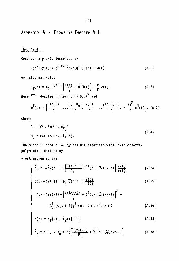
Theorem 4.1

Consider a plant• described by

A(q-l)y(t) = q-(k+l)boB(q'l)u(t ) + w(t) (A.l)

or• alternatively,

ef(t) = boq-(k+l) ) + 8T~(t) +

Here '-' denotes filtering by Q/TA M and

= Fu(t-l) u(t-nu) y(t) y(t-ny+l) ~T(t) L F . . . . . - T ' - T . . . . . P

(A.2)

!B M uM(t)], (A.3) P

where

n u = max (m+k, nP2 )

ny = max (n+n T-k, n).

The plant is controlled by the DSA-algorithm with fixed observer polynomial, defined by

- estimation scheme:

(A.4)

^ ^ ] ¢( t ) bo(t) =bo(t-l)+IT(t-k-l)+sT(t-l)~(t-k-l) r(t) L Pl

B(t) =O(t-l) + 6 O~(t-k-l) ~(t_) r(t)

2 r(t} =~r(t-]) +~u(t-k,.l_) + ~T(t_l)~(t_k_])] +

l Pl

+ B~ l~(t-k-l)l 2+~; O(~<l; a~O

(A.Sa)

(A.5b)

(A.5c)

c(t) = ef(t) - ~f(t l t- I )

~f( t l t - l ) = Bo(t-l)F~(tzk~ l) L P1

+ BT(t-l)~(t-k-l)]

(A.5d)

(A.5e)

112

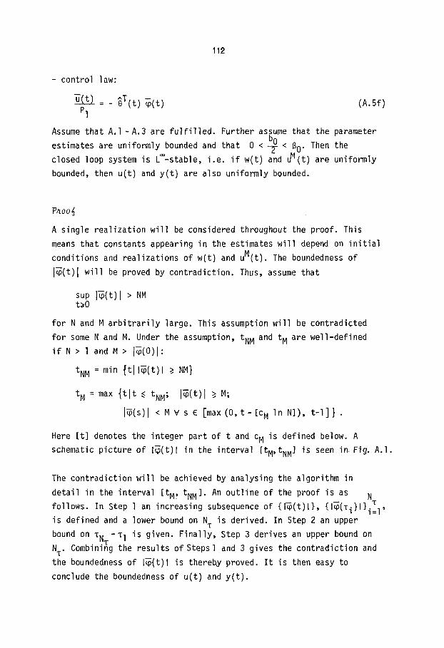
- contro l law:

~ ( t ) = _ ~T(t ) ~ ( t ) (A.5f) P1

Assume tha t A . I - A . 3 are f u l f i l l e d . Further assume tha t the parameter ~nb

estimates are un i formly bounded and that 0 < r-~-< B0" Then the

closed loop system is L~-stable, i . e . i f w(t) an-d uM(t) are un i formly

bounded, then u( t ) and y ( t ) are also un i formly bounded.

P~oo~

A single realization wil l be considered throughout the proof. This

means that constants appearing in the estimates wil l depend on in i t ia l

conditions and realizations of w(t) and uM(t). The boundedness of

l~(t)l wil l be proved by contradiction. Thus, assume that

sup ] ~ ( t ) l > NM t)O

fo r N and M a r b i t r a r i l y large. This assumption w i l l be contradic ted

fo r some N and M. Under the assumption, tNM and t M are we l l -de f ined

i f N > l and M > I~ (o ) I :

tNM = min { t i l ~ ( t ) l ) NM}

t M = max { t l t ~ tNM; i ~ ( t ) l ~ M;

l~ (s ) ] < M v s E [max (0, t - [ c M In N]) , t - l ] } .

Here [ t ] denotes the in teger part of t and c M is defined below. A

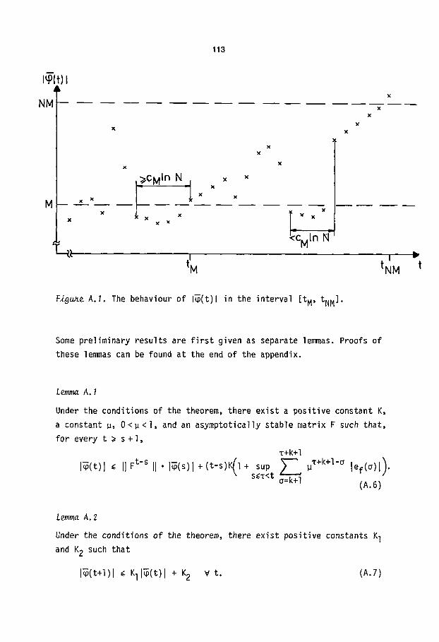
schematic picture of i~(t) l in the interval [tM, tNM] is seen in Fig. A.I.

The con t rad ic t i on w i l l be achieved by analysing the a lgor i thm in

de ta i l in the in te rva l [tM~ tNM]. An ou t l i ne of the proof is as N

fo l lows. In Step 1 an increasing subsequence of { l ~ ( t ) l } , { l ~ ( T i ) l } T i = l '

is defined and a lower bound on N T is der ived. In Step 2 an upper

bound on T N - T 1 is given. F i n a l l y , Step 3 der ives an upper bound on

N . Combining the resu l t s of Stepsl and 3 gives the con t rad ic t i on and

the boundedness of l~( t )1 is thereby proved. I t is then easy to

conclude the boundedness of u ( t ) and y ( t ) .

113

m itp(t

NM ¸

M

T

X X

X

,~CMln N

- - I X X

_1 X x

x

X :<

X

~CMln

X

X

I

INM

Figure A.I. The behaviour of l~(t) l in the interval [ t M, tNM].

Some preliminary results are f i r s t given as separate lemmas. Proofs of

these lemmas can be found at the end of the appendix.

Lemma A. I

Under the conditions of the theorem, there exist a positive constant K,

a constant ~, 0<~ < ], and an asymptotically stable matrix F such that,

for every t ) s + l ,

T+k+l

l~(t)l , II Ft-s II" l~(s)l +(t-s)K(l + sup ~ pT+k+l-~ lef(~)l). s~z<t ~=k+l

(A.6)

Lemma A.2

Under the conditions of the theorem, there exist positive constants K l

and K 2 such that

l~(t+l)I ~ Kii~(t)1 + K 2 V t. (A.7)

114

Lemmc A. 3

Under the conditions of the theorem, there exist positive constants

K 3 and K 4 such that, for k ~ l ,

( min K4l~(s) l ) ^ sup Jc(S)J. (A.8) J e f ( t l t - l ) J ~ K 3 +

t - 2k - I ~ s ~ t - k -2 t - k ~ s ¢ t - I

Before we re turn to the proof , we w i l l make the d e f i n i t i o n of t M

complete by de f in ing

1 2 ) (A.9) c M : max In ( I / p ) ' In(I/~)

where p is from Lemma A.I. I t is meant that c M = I / In( I /p) i f L=O.

Let [si,s 2] be any interval between t M and tNM such that

l (s)l < M v s I ~ s ~ s 2

I (s2+I)I M.

Assuming min I~(s) l is a t ta ined fo r s =s o , s I ~ s ~ s 2

s2-so+l / s2-s 0 s2-s O- M ~ J~(s2+1)l ~ K 1 (~(So)( + [K 1 +K 1

s2-So+I/ K 2 ), KI [l (so)l + K l - I

Lemma A.2 gives

1 \

+ . . . + l ) K 2

where i t has been assumed tha t K 1 > I , which is no r e s t r i c t i o n . The

d e f i n i t i o n of t M then impl ies

M K2 M K2 M K2 l~(So)J ~ s2-so+l - Kl---~i-1 ~ ~ K I -1 - In K I ' - K1 1

K 1 K 1 N cM -

and so, since the i n te rva l [Sl ,S 2] is a r b i t r a r y , we have fo r large N

M ~ K 2 1N 3 (A.lO) min I~(s) I ~ c M InK 1 K I - I ~ 2 ' tM~s~tNM N

where M has been chosen as

M N p ^ N cM In KI+3

: = (A.l l)

115

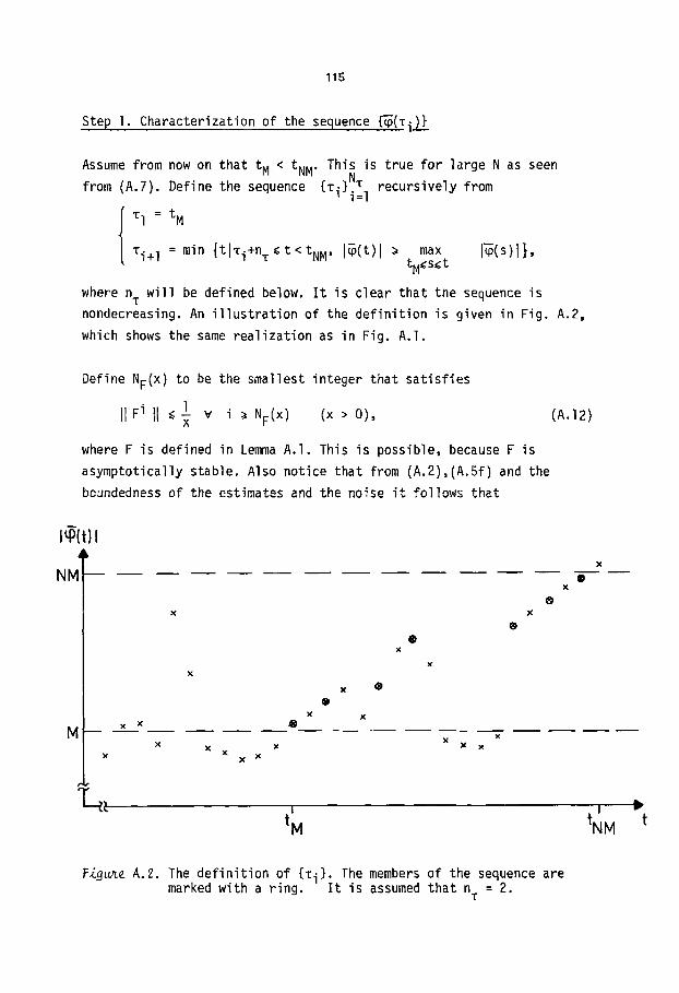
Step I . Character izat ion of the sequence { ~ ( ~ i ) }

Assume from now on that t M < tNM. This ~ is t rue fo r large N as seen

from (A.7). Define the sequence {~ i }~ l_ recu rs i ve l y from

{~1 = tM Ti+ l : min { t l T i+n ~ ¢ t < tNM, l~(t)] ~ max

tM~s~t

where n w i l l be defined below. I t is c lear tha t the sequence is

nondecreasing. An i l l u s t r a t i o n of the d e f i n i t i o n is given in Fig. A.2,

which shows the same r e a l i z a t i o n as in Fig. A . I .

Define NF(X ) to be the smal lest in teger tha t s a t i s f i e s

1 v i ) (x > 0) I] Fi II ~ ~ NF(X) ,

where F is defined in Lemma A . l . This is poss ib le , because F is

asympto t ica l l y s tab le. Also not ice tha t from (A .2 ) , (A .5 f ) and the

boundedness of the estimates and the noise i t fo l lows tha t

(A.12)

IL0(t) I

NN

Iv x × ®

x

0 x x

x

®

@

x"

X X X x X

x X x

X

@

I

t M

@ X

I

tNM

Figure A.2. The d e f i n i t i o n of {~i } . The members of the sequence are marked wi th a r ing . I t is assumed tha t n : 2.

T

116

lef(t+k+l) I ~ Kel~(t) I + K v

for some constants K e and K v. Now choose n T

satisfies the following three conditions:

( i ) n T ~ NF(4 )

as an i n t e g e r which

(A.13)

( i i ) n T ) k (A.14)

nT-k I - ( i i i ) nz1~ ,< 8K(Ke+I) .

Choose N so that

M ~ max , K 2

with K l and K 2 from Lemma A.2; i t is assumed that K l > l , which is no

restriction. This can of course be achieved with an N large enough.

Conditions like this one on N and M wil l appear several times in the

sequel. I t is then important to check that the constants appearing in

these conditions do not depend on the interval under consideration and

consequently on N and M themselves. This will however not be pointed

out every time i t appears.

I f N is chosen as above, Lemma A.2 and the definition of {zi } give

J~(Ti+l) j c KII~(Ti+I-I)I + K 2 ~ K 1 sup I~(t)J + K 2 Ti~t~Ti+n T

n +l n n -1 KIT l~(~i) I + (KIT + KiT + .. . + I) K 2

nT+l / K 2 n +I

Kl + KI_I) 2Kl+ I t follows in the same way that

n +1 I~(tNM) I ~ 2KIT I~(~ N )I

T

and so, combining these inequalities,

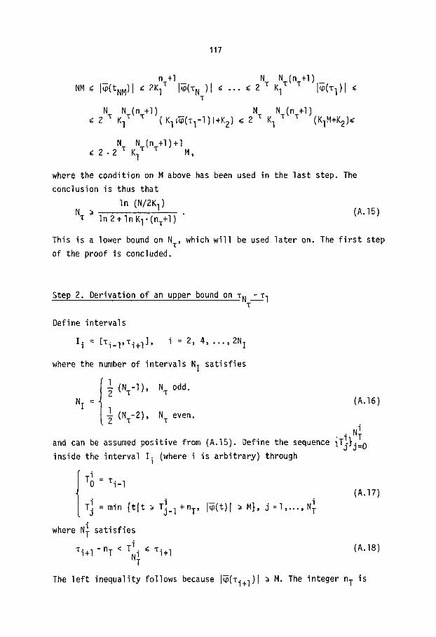
117

n +I N NT(nT+I ) NM ~ I~(tNM) I ~ 2KIT I~(T N )I . . . ~ 2 T K1 l (Tl) I

T

N N ( n + l ) N N (nT+l) 2 ~ K 1 ( K I I ~ ( T I - I ) I + K 2 ) ~ 2 T K1 (KIM+K2) ~

N NT(nT+l)+l 2 • 2 T K1 M,

where the cond i t i on on M above has been used in the l a s t s tep, The

conc lus ion is thus t h a t

In (N/2K 1 ) N ~ (a.15)

T In 2 + In K I . (n~+l )

This is a lower bound on N T, which w i l l be used later on. The f i r s t step

of the proof is concluded.

Step 2. Derivation of an upper bound on ZN -T l T

Define intervals

I i = [%i_ l ,T i+ l ] , i = 2, 4 . . . . . 2N I

where the number of intervals N I sat is f ies

1 ( N - I } , N odd.

N I = ] even. (NT-2)' N T

N i i T and can be assumed posit ive from (A.15). Define the sequence {Tj} j= 0

inside the interval I i (where i is arbi t rary) through

i TO = z i - I

T! = min { t l t ~ T i i j j - I +nT ' I (t)I ~ M}, j : 1 . . . . . N T

i s a t i s f i e s where N T

Ti+ 1 - n T < T i N~ ~ i+ l

(A.16)

(A.17)

(A.18)

The l e f t inequal i ty follows because I~(Ti+l) I ~ M. The integer n T is

118

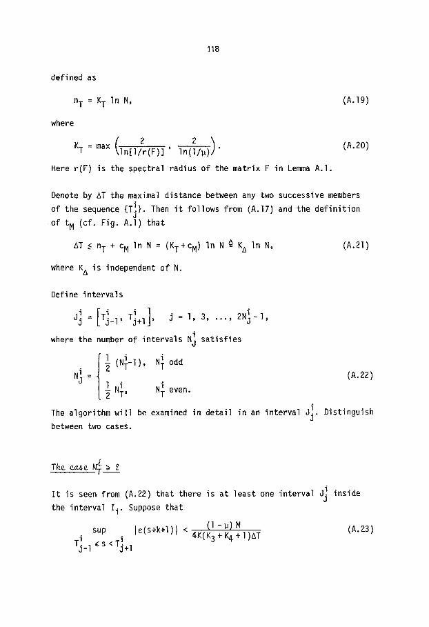
defined as

n T = K T In N, (A.19)

where

K T = max I n [ I / r ( F ) ] ' I n ( I / ~ ) " (A.20)

Here r (F) is the spectra l radius of the matr ix F in Lemma A . I .

Denote by AT the maximal distance between any two successive members

of the sequence { T ] } . Then i t fo l lows from (A.17) and the d e f i n i t i o n

of t M (c f . Fig. A . I ) tha t

AT < n T + c M In N = (KT+CM) In N A__ KA In N, (A.21)

where K A is independent o f N.

Define intervals

J j : j - l ' j + l ' J = I , 3 . . . . . 2N - I ,

i s a t i s f i e s where the number of i n te rva l s Nj

1 (N~- I ) , i N T odd i (A.22) Nj =

l i i NT, N T even.

The a lgor i thm w i l l be examined in de ta i l in an i n te rva l J ! . D is t ingu ish J between two cases.

The case N~T ~ 2

i ins ide I t is seen from (A.22) that there is at leas t one in te rva l Jj

the i n te rva l I i . Suppose that

sup i~ (s+k+ l ) i < ( I - I J ) M (A.23) T i i 4K(K3 + K4 + 1 )AT j - I ~ s < Tj+ 1

11g

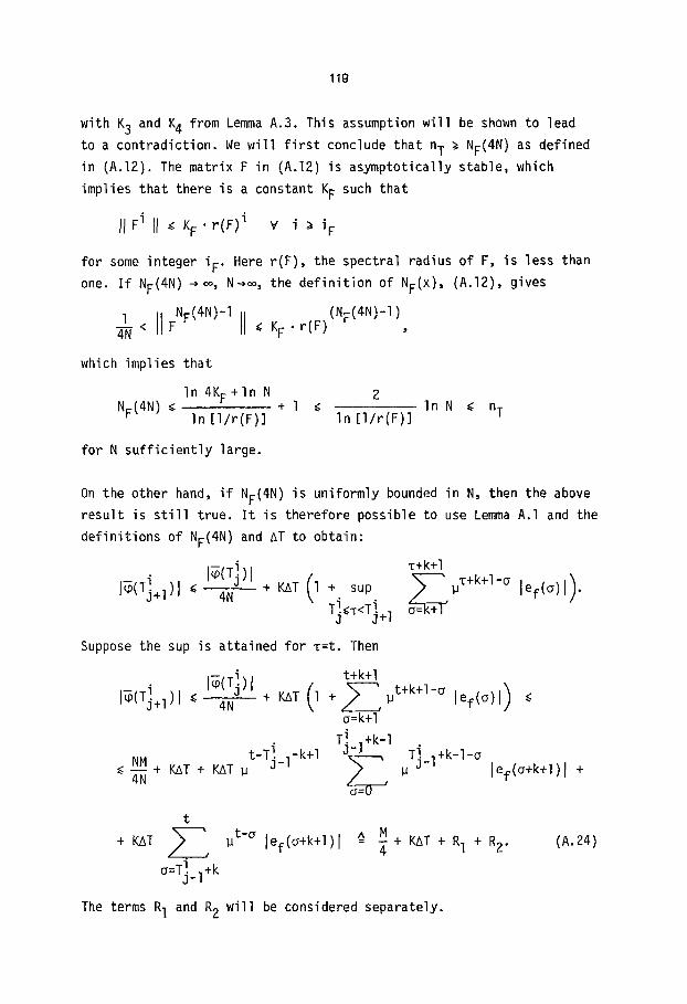
with K 3 and K 4 from Lemma A.3. This assumption will be shown to lead

to a contradiction. We will f i rs t conclude that n T ~ NF(4N ) as defined in (A.12). The matrix F in (A.12) is asymptotically stable, which

implies that there is a constant K F such that

II Fi II ~< K F' r (F) i V i ) i F

for some integer i F . Here r(F), the spectral radius of F, is less than one. I f NF(4N) -*~, N-*~, the definition of NF(X). (A.12), gives

1 i FNF(4N)-I (NF(4N)-I) 4N < II ~ K F- r(F) ,

which implies that

In 4K F +In N 2 NF(4N ) ~ + 1 ~ In N ~ n T

In [I /r(F)] In [ I /r(F)]

for N sufficiently large.

On the other hand, i f NF(4N ) is uniformly bounded in N, then the above result is s t i l l true. I t is therefore possible to use Lemma A.l and the definitions of NF(4N ) and AT to obtain:

- i I~(T~)I T+k+l I~P(Tj+I)I~ 4---T--+ KAT ( l + sup ~ I ~ T+k+l-° lef(a)J).

Ti~'T<Ti+I 3 J

Suppose the sup is attained for T=t. Then

]~(T~+I)] "< 4 - T + KAT

t-T~_ l-k+l NM -<-~T_ + KAT + KAT ~N

t+k+l + ~ - ~ , l j t+k+l-~ ,ef(a), 1 .<

a=k+l

T~.]+k-I Ti-l+k-l-a ~ [ef(a+k+l) i +

t

+ KJ~T ~ - - ~ t - a ief(a+k+l) I

a=T~_l+k

M + KAT + R 1 + R 2. (A.24) 4

The terms R 1 and R 2 will be considered separately.

120

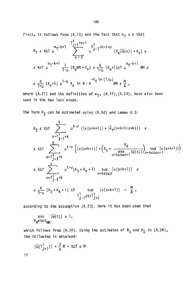
First , i t follows from (A.13)and the fact that n T ~ k that

T]-l+k-l~. T] l+k-I nT-k+l _ -a R 1 ~ KAT ~ ~ ~ (Kel~(~)I + Kv)

nT_k+l nT-k+l 1 (KeNM+ Kv) ~ (Ke+I)AT ~ NM KAT ~ ~j~

-K T In (I/~) M (Ke+l) 1 - k KA In N.N NM ~ ~ ,

where (A.21) and the def in i t ion of n T, (A.Ig),(A.20), have also been used in the two last steps.

The term R 2 can be estimated using (A.5d) and Lemma A.3:

t R 2 ~ KAT ~__~ t - ~ (IE(a+k+1)l + lef(a+k+llo+k)i)

~=T]_l+k t

~ KAT ~ - - ~ IJ t-~ [i~(~+k+l)i +(K3+

~=T]_l+k t

, ut-~(K3 < KAT +K 4+I) sup i~( s+k+l)I -< , / ( ~ - k ~ s . < ~

~=Tj_l +k

K 4 min

o-k~s~o-I

K M .<-~_~ (K3+K4+I) AT sup i~(s+k+l)[ < ~ , T i .<s<T]+ 1 j - l

according to the assumption (A.23). Here i t has been used that

! sup I~(s+k+l)l]( I~(s) /a-k~s(o-I

min I~(t) l ~ l, tM~t~tNM

which follows from (A.IO). Using the estimates of R 1 and R 2 in (A.24), the following is obtained:

- i 3 . , ..l~(Tj+lll < - M + KAT ~ M 4

i f

1 2 1

M N P FAT ~ -

4 4

This condi t ion is t r i v i a l l y sa t i s f i ed fo r large N as seen from (A.21). - i We have thus arrived at a contradiction since J~(Tj+I) I ~ M by

construction. I t is possible to conclude that

sup J~(s+k+l)J ~ (l-p) M (A.25) i i 4K(K 3 + K 4 +1)AT Tj-I~S<Tj+ 1

i This inequality is valid for all intervals dj.

Define

b o v(t) = 5~(t) +~oo l~(t)12 (A.26)

and suppose the supremum in (A.25) is obtained fo r s = t , Lemma 4.2

then gives

T]+ 1 +k T!+I +k V(T~+I+k)-V(T ~ l + k ) ~ - c F l ~2(s) 1 ~ - ~

- r ( s ) + c ,

s:T _l+k+l s:T]_l+k+l i

2 Tj+I-1 ~2(t+k+l) K v

- c + ~ " 1 - - $

r ( t+k+ l ) c . i r ( s+k+ l ) / s=T! .

3-I

where K v is the bound on the noise in (A.13). I t fo l lows from (A .5c , f ) i T i and the boundedness of the estimates tha t , for Tj_ 1 ~ t < j + l '

t ~t-s 2 r ( t+k+ l ) .< r ( k+ l ) + T ~ + Kr z J~(s)J .< s=0

K r 2 K r .< r (k+ l ) + ~ +~Z~ (NM)2 -< ~ (NM) 2,

fo r some K r i f N is chosen s u f f i c i e n t l y large. Furthermore, from (A.5c)

and (A. IO) a lower bound on r ( t ) can be obtained:

l ~ ( t ) J 2 2 1 N 6 (A.27) r ( t+k+ l ) Bu >. •

I f these two resu l ts are used above, the fo l lowing inequa l i t y is

1 (R~(s ) )2 r (s )

1 2 2

obtained:

V(Tj+ 1 +k) - V(Tj. 1 +k) .< c (1 -~ . )

2Kr(NM)2

2 2AT K v . 4

e2(t+k+l) + - ~ 6 ~ N 6

and so, using (A.25), we have for N s u f f i c i e n t l y large:

V(T]+ 1 +k) - V(T~_ l + k ) .<

_ c(l-k) . ~ (l-w) M ~2 8~T K 2 + v 2Kr(NM)2 \4K(K3+K4+I)AT) c 6~ N6

2 8AT K v c ( l -~ ) (I-~12 + - -

"<- N2AT 2 2Kr[4K(K3+K4+I 112 C 6~ N 6 A_

^ c I c 2 AT - 1 + (A.28)

N 2 &T 2 - ~ ,

where c I and c 2 are independent of N.

Use the estimate of AT in (A.21) to obtain

c I c2K A In N + .<

N2K2(1 n N) 2 N 6

co ,< - ~ - ~ - N2 "< N4

for N s u f f i c i e n t l y large. Here c O is independent of N. This inequa l i t y i i t imes. Thus holds for every interval Jj, i.e. Nj

,

But V is pos i t ive and bounded. I f the bound is denoted by Kv' we have

i Kv . N 4. (A.29) Nj ~-00

1 2 3

The case N~ < 2

I t is seen from (A.22) that in this case N~ : 0. Consequently, (A.29) is t r i v i a l l y sat isf ied.

The conclusion is thus that (A.29) is valid in every interval I i , provided N is chosen large enough. The inequality (A.18) and (A.22) imply

_ T i T i _ T i T i+l 2N~ = (T i+ I -T i 'N~ )+ (N~ 2NJ ) "< n T+AT <̀ 2AT,

and so, by using (A.29),

_ T i . T i _

Kv 4Kv ,4. .<,AT+ 2N~AT .< 2AT (l +~-~0 N4),< T O AT.

Summing for i -- 2,4 . . . . . 2N I gives

4Kv N 4 T2NI + l - T l ~ -~0 AT- -NI,

which ends Step 2 of the proof.

(A.30)

Step 3. Derivation of an upper bound on N and the contradiction T ' "

Consider an interval I i defined in Step 2. Suppose that

(l-p)l~(Ti+l) I sup l~(s+k+l)l <

Ti+l-2nT~ s < Ti+ l 4KnT(K3+K4 +l ) (A.31)

This w i l l lead to a contradiction in the same way as in Step 2. Thus, analogously with (A.24) we have

l~(Ti+l- n) l l~(Ti+ l ) l ~ 4 + KnT + R1 + R2'

where

124

Ti+l-2nT+k-I t-Ti+l+2n~-k+l o = ~ ~i+l-2nT+k-l-~

R l = Kn T ~ ~ lef(a+k+l) l

t

R2 = Knz ~=Zi+l~- nT+k t - o lef(o+k+l) I

and t is in the interval [Ti+l-n T, mi+l-l]. Notice that the property (A.14i) of n has been used.

Let [t] denote the integer part of t and estimate R l by using (A.13) and the inequality K v ~ M = N p, which is valid for N large enough:

R 1 ~ Kn ~nT-k+l[ T i+l-2nT+k-l-(tM-[cMlnN]-l)

tM-[C M In N]-I , tM-[C M In N] - l -o

• ~ lef(~+k+l) l + /

O=0

Zi+l-2nT+k-I Ti+l-2nT+k- l -o

+ ~ - ~ , p lef(o+k+l)l] ¢ ~=tM-[C M In N]

n-k+l [ [CMlnNl+k NM + l~(Ti+l)I ] Kn T ~ T (Ke+l) I - , i - ~ '

where (A.14 i i ) has been used in the last step. Now use (A.9) and (A.14 i i i ) to obtain

n -k [ M I~(Ti+l )I ] R1 .< Kn T ~ T (Ke+l) l + 1-~ "<

n -k 2 l~(Ti+l )I Kn T ~ T (Ke+l) ~-~ l~(Ti+l)l ~ 4

The term R 2 is estimated as in Step 2 using the assumption (A.31):

K3+K4 +I I~(Ti+l)l • sup l~(s+k+l)l < 4

R 2 ~ Kn I-~ ~i+1-2nT~ S < ~i+l

Insert the estimates of R l and R 2 above, which gives

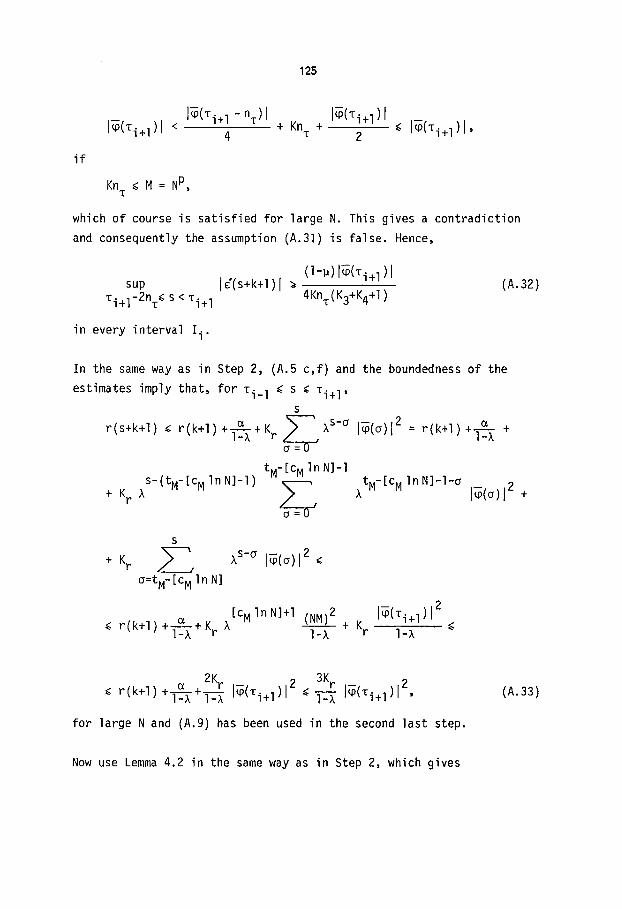
125

i f

l~(~i+ l - nT)l l~(Ti+l)l J~(Ti+l) j < + Kn + ~ l~(~i+l) I, 4 T 2

Kn ~ M = N ~, %

which of course is satisf ied for large N. This gives a contradiction and consequently the assumption (A.31) is false. Hence,

( I -~) l~(Ti+ l )I sup JC(s+k+l)J ~ (A.32)

Ti+l-2n ~ s < Ti+l 4KnT(K3+K4+I)

in every interval I i .

In the same way as in Step 2, (A.5 c, f ) and the boundedness of the

estimates imply that, for Ti_ 1 ~ S ~ Ti+ I , S

r(s+k+l) ~ r(k+l)+l_-~+Kr _ _ ~ s'a J~(a)J 2 = r(k+l)+T~_~ +

tM-[C M In N]-I + Kr xs-(tM-[CM In N]-I) o = ~ tM-[C M In N]- l-a

I~(a)l 2

S

+ Kr ~ , ~s-o j~(a)J2

a=tM-[C N In N]

[CM In N]+I (NM) 2 J~(Ti+l) J 2 r(k+l)+--~-~ +K r ~, + K r I-~ I-~ I-~

2Kr 2 3Kr r(k+l)+-F~+ZZ~ J~(Ti+l) j ~-fZ~ J~(Ti+1)J 2'

for large N and (A.9) has been used in the second last step.

(A.33)

Now use Lemma 4.2 in the same way as in Step 2, which gives

126

Ti+l - l 2 ~2(s+k+l) K v

V(Zi+l+k) - V(Ti_ l+k) ~ - C > " + , r (s+k+l ) c

s=Ti_ 1

K 2 ~i+1 - I E2(t+k+l) + v ~ 1

- c r ( t+k+ l ) ~ - " / / , r (s+k+l ) ' s=Ti_ 1

Ti+ 1 - I

7-" / r(s+k+l ) s=~i - I

where the supremum in (A.32) is attained for s = t. Using (A.32), (A.33),

and (A.27) we have for N large enough:

4K~ Ti+l - T i - l ^ V(Ti+l+k) - V(Ti_1+k) ~ - C - ( -p 2 I-,~, 1 ~ f ~ 2 + "

[4KnT(K3+K4+I)] 3K r ~ N 6

^ Ti+l -T i_ I = _ c 3 + c 4 • N6 '

where c 3 and c 4 are independent of N. The inequal i ty is val id for

i = 2, 4 . . . . . 2N I and so

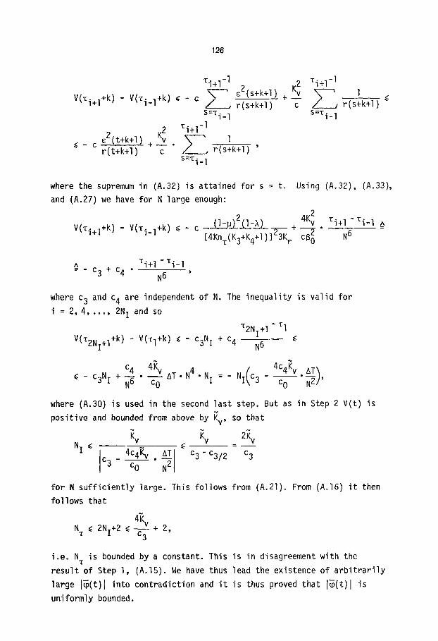
V(T2NI+I+k) - V(T]+k) ~ - c3N I + c 4 N6 T2NI+I -T1

c4 4Kv N 4 ( 4C4Kv A T e , - c3N I + N-- 6 • ,c0 AT, -N I = - N I c 3 - c T N2 /

where (A.30) is used in the second last step. But as in Step 2 V(t) is

posit ive and bounded from above by K v, so that

Kv Kv 2Kv - - ~<[ -

NI "< _ 4c4Y, v • A__~T c 3 -c3/2 c 3 c 3 c o

for N su f f i c ien t l y large. This follows from (A.2I). From (A.16) i t then

fol lows that

N'r "< 2NI+2 "<-~3 + 2,

i .e . N is bounded by a constant. This is in disagreement with the T

resul t of Step l , (A.15). We have thus lead the existence of a r b i t r a r i l y

large l~( t ) I into contradiction and i t is thus proved that l~(t) l is

uniformly bounded.

127

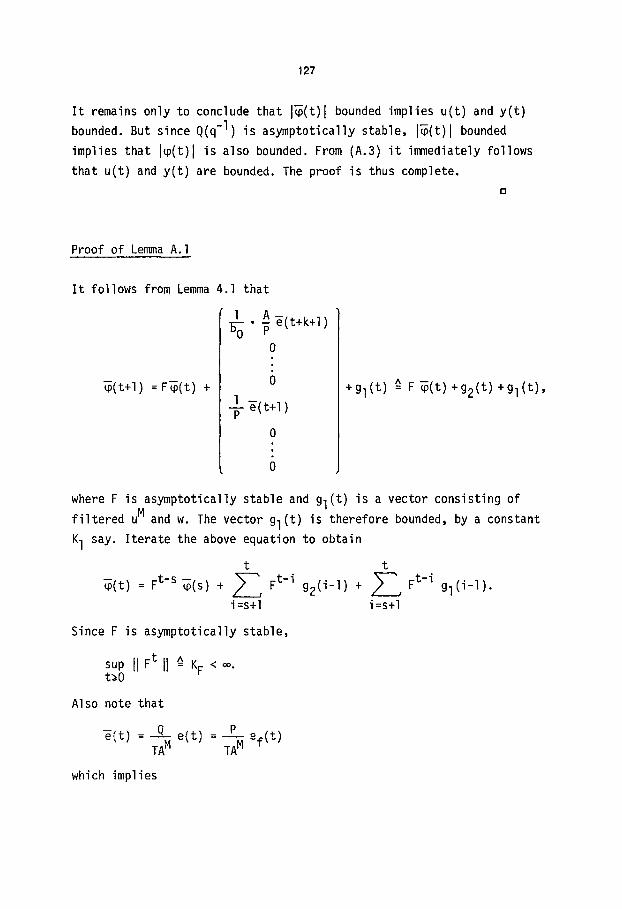
I t remains only to conclude that l~(t)l bounded implies u(t) and y(t) bounded. But since Q(q-l) is asymptotically stable, l~(t)l bounded implies that l~(t)l is also bounded. From (A.3) i t immediately follows

that u(t) and y(t) are bounded. The proof is thus complete.

Proof of Lemma A.I

I t fol lows from Lemma 4.1 that

~(t+l) =F~(t) +

1 A e ( t+k+ l ) N'5 0

6 1 g ( t + l )

-V 0

+ g l ( t ) ~ F ~ ( t ) + g 2 ( t ) + g l ( t ) ,

where F is asymptotically stable and g l ( t ) is a vector consisting of

f i l t e red u M and w. The vector g l ( t ) is therefore bounded, by a constant

K l say. I terate the above equation to obtain

t t ~ ( t ) : F t -s ~(s) + ~ - - " F t - i g2 ( i - l ) + ~ F t - i g l ( i - l ) .

i =s+l i =s+l

Since F is asymptotically stable,

sup II Ft II ~= KF < ~. t~O

Also note that

~(t) =-q-Qe(t) = PM TA M TA e f ( t )

which implies

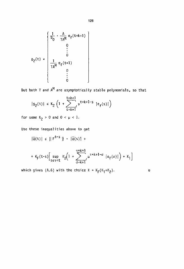
128

g2(t) :

I A ef(t+k+1) 'TA"

0 1 - ~ ef( t+ l )

O

0

But both T and A M are asymptotically stable polynomials, so that

t+k+l I g 2 ( t ) l ( K 2 ( I + ~ - ' ~ , t + k + l - s l e f ( s ) i )

s=k+l

for some K 2 > 0 and 0 < lJ < I.

Use these inequal i t ies above to get

l ~ ( t ) l ~ II Ft-s }l " l~(s) l +

+ KF(t-s)[ sup K211 - LS(T< t

~+k+l ~ - - ~ / l j T+k+l-~ l e f ( a ) I ) + KI] a=k#l

which gives (A.6) with the choice K = KF(KI+K2 ). a

129

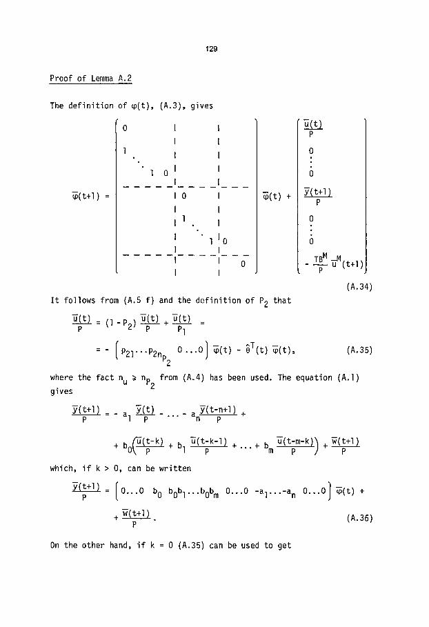
Proof of Lemma A.2

The def in i t ion of ~ ( t ) , (A.3), gives

0

1

~( t+ l ) =

1 0

1

~( t ) +

I t fol lows from (A.5 f ) and the de f in i t ion of P2 that

~( t ) ~( t ) -6(t) = ( l -P2 ) + - P P Pl

= - , FP21...P2nP2 0 . . . 0 l , ~( t ) - oT(t) ~ ( t ) ,

P

0

&

g( t+ l ) P

0

6 _ TBM u-M(t+l )

P

(A.34)

(A.35)

where the fact n u ~ nP2 from (A.4) has been used. The equation (A.I ) gives

y ( t+ l ) _ al y ( t ) y ( t -n+ l ) + P P - . . . - a n p

L ,/-u(t-k) + u ( t - k - l ) + . . . + b ~(t-m-k}~ + ~ ( t + l ) + D 0 \ p bl p m p / p

which, i f k > O, can be wr i t ten

y ( t + l ) = p [ 0 . . . 0 b 0 b0bl. . .bob m 0 . . . 0 - a l . . . - a n O. . .OI ~ ( t ) +

+ w(t+ l ) (A.36) P

On the other hand, i f k : 0 (A.35) can be used to get

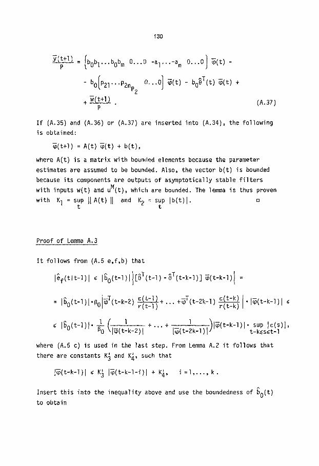
130

~(t+l) : p Ibobl...bobm D...O -al. . .-a n 0...0 1 ~ ( t ) -

^T - bo[P21...P2nP2 0...0] ~(t) - bOO ( t ) ~ ( t )

+ ~( t+ l ) P

+

(A.37)

If (A.35) and (A.36) or (A.37) are inserted into (A.34), the following is obtained:

~(t+l) : A(t) ~(t) + b(t),

where A(t) is a matrix with bounded elements because the parameter estimates are assumed to be bounded. Also, the vector b(t) is bounded because its components are outputs of asymptotically stable f i l ters with inputs w(t) and uM(t), which are bounded. The lemma is thus proven

with K 1 = sup JJA(t)JJ and K 2 = sup Jb(t)J. a t t

Proof of Lemma A.3

I t follows from (A.5 e,f,b) that

Jef(tlt-l)J ~ Ibo( t - l ) I I [oT( t - l ) -oT( t -k- l ) ] ~(t-k- l)}

r ( t - l ) r(t-k)

^ l ( l ÷ . . . + 1 ) "< Ibo(t-1)J'~O J~(t-k-2lJ l~(t-2k-llJ l~(tmk-lll-t_k.<s~t_isup l~(s)],

where (A.5 c) is used in the last step. From Lemma A.2 i t follows that there are constants K~ and K~, such that

J~(t-k-l)J ~ K~ J~(t-k- l - i )J + K~, i : I . . . . . k.

A

Insert this into the inequality above and use the boundedness of bo(t )

to obtain

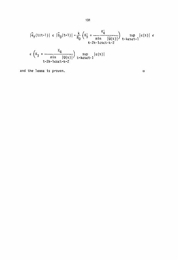
131

[ e f ( t l t - l ) l ~ Ib0(t-l)l .T0 K½ + min [~(s)l

t-2k-l.<s.<t-k-2

( "4 ) .< K 3 + sup l~(s)l

min IT(s)[" t-k.<s.<t-I t -2k- l~s~t -k-2

sup t -k~s~t- I

I~(s)l

and the lemma is proven. []

132

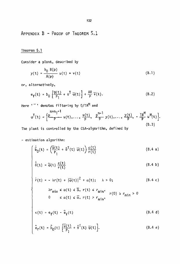
APPENDIX B - PROOF OF THEOREM 5,1

Theorem 5.1

Consider a plant, described by

b 0 B(p) y(t) - u(t) + v(t) (B.l)

A(p)

or, alternatively,

ef ( t ) = b 0 [ ~ p ~ + e T ~ ( t ) ] + - ~ ( t ) . (B.2)

Here ' - ' denotes f i l t e r i ng by Q/TA M and

p m+nT-I u(t) pn-l Y~.-..--!, TBM uM(t)]. J ( t ) = I-----F--- u(t) . . . . . T ' T y(t) . . . . . - T

(B.3) The plant is controlled by the CSA-algorithm, defined by

- estimation algorithm:

o(t) : \P]

~(t) ~(t) = ~(t) r ( t )

~(.t) (B.4 a) r ( t )

(B.4 b)

r ( t ) : - Xr( t) + l ~ ( t ) l 2 + ~ ( t ) ; x > O;

Xrmi n

0

e( t ) ~ ~, r ( t ) ~ rmi n,

~(t) ~ ~, r ( t ) > rmi n, r(O) ) rmi n > 0

(B.4 c)

~(t) = e f ( t ) - e f ( t ) (B.4 d)

Gf(t) : bo(t) ~ ( t ) + ~T(t ) ~ ( t ) ] . LP 1

(B.4 e)

133

- control law:

= _ [PI (°) BT(t)] ~(t). P1 t P1

(B.4 f )

Assume that assumptions A. I -A.4 are fu l f i l led. Further assume that the

parameter estimates are uniformly bounded. Then the closed loop is

L=-stable, i .e. i f v(t) and uM(t) are uniformly bounded, then u(t) and

y( t ) are also uniformly bounded.

Proof

A single realization wil l be considered throughout the proof. The

boundedness of l~(t)l wil l be proved by contradiction. Thus,

assume that

sup l~ ( t ) I > NM t~O

for N and M a r b i t r a r i l y large. This assumption w i l l be contradicted for

some N and M. Assuming the unboundedness, tNM and t M are wel l-def ined

i f N > l and M > I~(0) I :

tmM = min { t I l ~ ( t ) l : NM }

t M = max { t [ t< tNM; l~ ( t ) l = M;

l~(s) I <M v s E (max(O,t-c M l n N ) , t ) } .

Here the con t inu i t y of I~ ( t ) I i s used. The constant c M w i l l be defined

below. A typ ica l rea l i za t ion of I~ ( t ) l in the time in terva l [tM, tNM] is

shown in Fig. B. I .

The contradiction wi l l follow from thorough analysis of the algorithm

in the interval [tM, tNM]. An outline of the proof is as follows. In Nz Step l an increasing sequence ( l~(Ti) l } i= l in the interval [tM, tNM] is defined and a lower bound on N is given. Step 2 derives an upper bound

on ~N~-~I" Finally, Step 3 derives an upper bound on N T which is in

disagreement with the result in Step l and the boundedness of l~(t)l is

thereby proved. The boundedness of u(t) and y(t) is then easily

concluded.

134

ICPlt)I

NN

t M

I I I

I I I INM

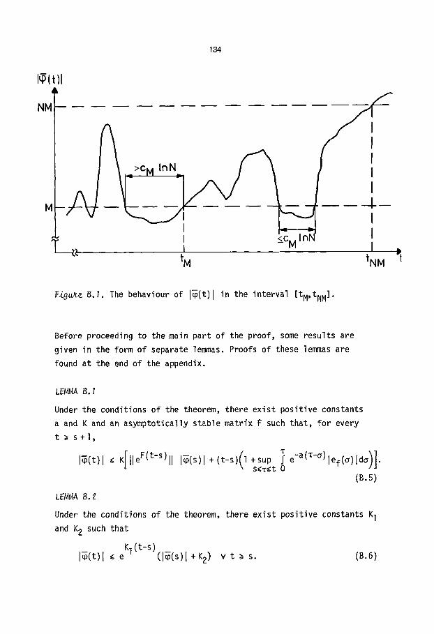
Fi~upte B.I. The behaviour of l~( t ) l in the interval [tM, tNM].

Before proceeding to the main part of the proof, some results are

given in the form of separate lemmas. Proofs of these lemmas are

found at the end of the appendix.

LEMMA B.I

Under the conditions of the theorem, there exist positive constants

a and K and an asymptotically stable matrix F such that, for every

t ) s + l ,

]~(t) l ~ K[lleF(t-s)ll

LEMMA B. 2

l ~ ( s ) I+ ( t - s ) ( l +sup ~ e-a(T-°) lef(~)Ido)]. s(T=;t 0

(B.5)

Under the conditions of the theorem, there exist positive constants K 1

and K 2 such that

K1 (t-s) (j~(s) J~(t)J ~ e J+K2) ¥ t ~ s. (B.6)

135

LEMMA B.3

Under the condi t ions of the theorem, there ex is ts a pos i t ive constant

K 3 such that

l~ ( t ) [ 2 - - ~ K 3 v t . (B.7)

r ( t )

LEMMA B. 4

Under the condi t ions of the theorem, there ex is t pos i t ive constants

K4, K5, and c such that for a rb i t r a r y T,

^ K1T t Jef ( t ) l ~ K 4 e-CTj~(t)J + K 5 e f JE(s)l ds V t >. T (B.8)

t -T

where K 1 is as in Lemma B.2.

Before return ing to the proof of the theorem, an important observation

w i l l be made. F i r s t choose

CM = m a x ( ~ , ~ ) (B.9)

wi th a from Lemma B. I . Let [Sl,S 2] be any in terva l between t M and tNM

such that

{ l (s2) l : M

l (s)l < M V s I < s < s 2.

I f

of t M give

Kl (s2-so) ( l~(So) M = J~(s2) j ~ e J

min l~(s)I is attained for s=s O , Lemma B.2 and the definition Sl~S~S 2

KIC M In N +K2) ~ e ( I~(So)l +K2)

which implies

l~(So) I ) M _ K2" NKICM

Since the interval [Sl,S 2] is arbitrary, we thus have

136

M K2" min l~(s) l ~ KlCM tM~ s ~ tNM N

(B.IO)

Step I. Characterization of the sequence {~(Ti)}

N T The sequence {Ti}i= l is defined recursively from

T = t M

Ti+ 1 : i n f { t I Ti+n ~ { t < tNM, l~ ( t ) l ~ sup l~ (s ) I } , tM~ s ~t

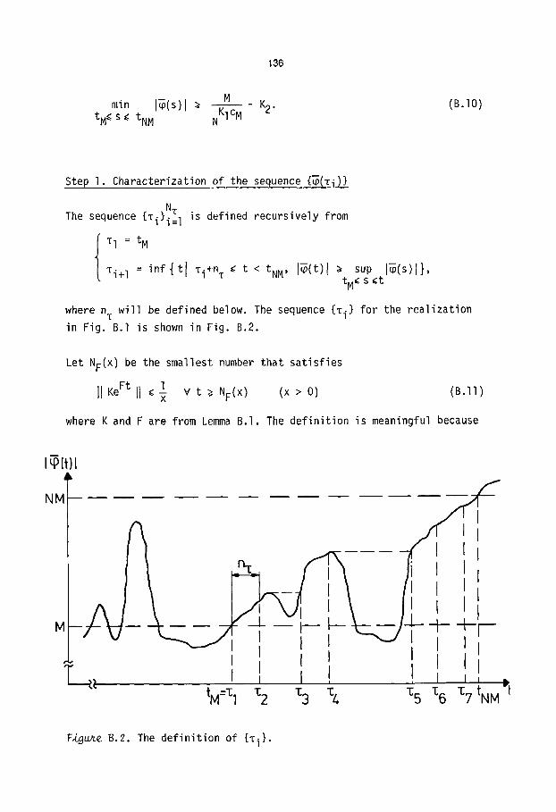
where n w i l l be defined below. The sequence {T i } for the rea l i za t ion

in Fig. B.I is shown in Fig. B.2.

Let NF(X ) be the smallest number that satisfies

V t ~ NF(X) (x > O) (B.l l) II Ke ~t II ~ x

where K and F are from Lemma B.l. The definition is meaningful because

NN

{t)

- I

I I I

tM=~l 1:2 1; 3 1;/.. 1:5 z6 z7 tNM "~t

Figure B. 2. The definition of {%i }.

137

F has i ts eigenvalues in the open le f t half plane. Also note that

from (B.2), (B.4 f ) , and the boundedness of the estimates and the

noise i t follows that for some K e, K v

lef ( t ) I ~ K e l~(t)I + K v V t. (B.I2)

Now choose n T in the definit ion of {T i } to be a number which f u l f i l l s

the following conditions:

( i ) n T >~ I

( i i ) n T ~ NF(5 )

an t

( i i i ) n e 2 .~ T 10K(Ke+l)

cn T 2 a ( i v ) n e .<

T 5KK 4

(B.13)

Here a and K are from Lemma B.l, K e as in (B.12), and c and K 4 from

Lemma B.4.

Let M satisfy the condition

M ~ K 2

with K 2 as in Lemma B.2. I t should be noted that N and M can be chosen

arbi t rar i ly . A number of conditions of the type above wil l appear in

the proof. They are however easy to f u l f i l l by choosing N and M

appropriately. I t is, however, important that the constants appearing

in the conditions do not depend on the choice of interval [tM, tNM],

i .e. on N and M themselves. This fact wil l not be commented upon in the

sequel.

I f M is chosen to f u l f i l l the condition above, Lemma B.2 gives rise to

an inequality in the following way. Separate between two cases:

(i) Ti+ 1 = T i + n T ; then

l~(Ti+l)l ,< 2e KInT }~(Ti) I .

138

( i i ) z i+ 1 > Ti+n ~ ; the de f i n i t i on of {Ti } then implies

l~(Ti+n )I < sup I~(s)I • i ~ S~Ti+n T

and the continuity gives

]~(Ti+l) I : sup I~(s)l ~ 2e Kln~ l~(Ti) I . TiE S~Ti+n T

The same inequality thus holds in both cases. Using this together

with the fact that

tNM T N < n T,

which follows from the definition of {T i } and the continuity, the

following is obtained:

Kin T NM = (~(tNM) I ~ 2e

NT e KI nTN =2 TM

N eKlnN I ; ( ~ N ) I ~ . . . ~ Z T ~ :

which implies

N T

I n N In 2+Kln T

(B.14)

This is the lower bound on N T sought for in Step I .

Step 2. Derivat ion of an upper bound on T N - T 1

Define in terva ls

I i = [Ti_l ,Zi+l ] , i = 2,4 . . . . . 2N I

where the number of in terva ls N I sa t i s f i es

(N r - I ) , N odd

NI = 1 2), N even. (NT T N i

i T Consider an in terva l I i and define the sequence {T j } j= 0

(B.15)

inside the

139

i n te rva l through

TO = ~i-I (B.16) i i

T~j = min{ t I t ~ Tj_ l+n T, l~(t)l ~ M}, j =I . . . . . N T

where N~ satisfies

Ti+l - nT ~ Ti (B.17) i ~ ~i+l" N T

The lef t inequality follows because l~(Ti+l) I ~ M. The constant n T is

defined as

n T = K T In N, (B.18)

where

KT = max ( - r - ~ ' ~ p ) " (B.19)

Here r (F) is the la rges t real par t of any eigenvalue of F and p is

defined as

a p = ,

a + c

i and T i Let AT be the maximal distance between any Tj j + l "

the d e f i n i t i o n of t M (cf , Fig. B.1) and (B.16) t h a t

AT .< n T + c M In N = (KT+CM) In N A KA In N,

(B.20)

I t follows from

(B.21)

where K A is independent of N.

Define i n t e r va l s

i j Tj+,I Jj = IT -l J = l , 3 . . . . . 2N - I ,

where the number of intervals NJ satisfies

I i odd i 2 ' NT ' (B.22)

Nj = ½ i i N T , N T even.

i w i l l now be examined. The behaviour of the a lgor i thm in an i n te rva l J j

140

D is t ingu ish between two cases.

Z Tk~ ~ N T >.

i in the From (B.22) i t is seen tha t there is at leas t one i n te rva l Jj

i n te rva l I i . Suppose that

T i j + l

I i rj_l

M I ~ ( s ) l ds < . (B.23)

4K ( l + - ~ ) AT e KlpnT

This w i l l lead to a con t rad ic t i on . To see t h i s , we w i l l f i r s t show

tha t n T ~ NF(4N ). The matr ix F used when def in ing NF(X ), ( B . I I ) , has

i t s eigenvalues in the open l e f t ha l f plane. This impl ies the existence

of a constant K F such tha t , fo r some t F,

II eft II ~ K F et'r(F) V t ~ t F,

where r(F) is defined in connection wi th (B.19). Clear ly NF(4N ) ~ ,

N ~ . Then i t fo l lows by c o n t i n u i t y of II eFt II from ( B . I I ) that

FNF(4N)II NF(4N)'r(F) 1 K I Ie ~ KK F e 4N

fo r N s u f f i c i e n t l y large and so

In N + In 4KK F 2 NF(4N) ~ - r (F ) ~ _ - ~ In N ~ n T.

I t is thus possib le to use Lemma B.I and the d e f i n i t i o n s of NF(4N ) and

AT to obtain

-- i I~(T] )1 (I T]~$~TJ +I i£°(Tj+l)] ~ 4 ~ + KAT + sup ~ e-a(~-°)lef(~)l do). i 0

Suppose the sup is a t ta ined fo r • = t . Then

• I ~ ( T ! ~ I t i~(T~+l) i ~ .< ' " 3 " 4 ~ + K~T (I + f e - a ( t - ° ) l e f ( a ) i do) .<

0

141

i +T j +T-q) NM -a(t -T _l-T) T j - I -a(T - I ~TN + KAT+KAT e S e lef (o) l do +

0

t + KAT . I e-a(t-~)lef(~)l d~ ~ ~+KAT4 +Rl +R2' (B.24)

T~ _ l +T

where 0 < T < n T w i l l be chosen later . The two terms R 1 and R 2 w i l l be estimated separately. From (B.12) and the def in i t ion of {T~} i t fol lows that

-a(nT-T) 1 R 1 ~ KATe

-a(nT-T) 1 KATe

i f N and M are chosen such that K v (B.4 d) and Lemma B.4:

a suP. lef (°)1 ~ o~T~

-a(nT-T ) K (Ke+l) AT e NM, sup(Kel~(~) I + K v) ~

o~T~

NM. The term R 2 is estimated using

t T~ +I

T~ I+T T i j - I

t KI T o )Ids) d° + KAT[ I e-a (t-~)lK4e-CTl~(°) I + K5e I IE(s ]

o-T T~_ 1 +T i

Tj+l ( K5 eKIT) I K -cT .< KAT I +-~- IE(s)Ids + ~ K4AT e NM.

T j - I

Now choose T = p.n T and use (B.20) to obtain for large N

KAT ( -a(l-p)nT "cpnT) Rl + R2 " < T (Ke+l) e + K 4 e NM +

T +I ( I I + KAT 1 + - a eKlpnT I (s)l ds

T i j-1

I (o)I do +

142

i T j+1

-cpnT NM (1 +-~) e KlpnT KAT (Ke+K4+I) e + KAT rj " < T T i j - I

-CpKTln N

I (s)l ds <

<_K (Ke+K4+I) KA In N e a M M (B.25) NM + ~ ~ ~ ,

where (B.18), (B.21), and the assumption (B.23) have been used in the second last step and the definition of K T, (B.19), was used in the last step. I f (B.25) is inserted into (B.24), the result is

I~(T]+l) I < M

i f

M KAT ,< - 4

This is t r i v i a l l y satisf ied for large N by the choice

M = N p A= NKI (CM + PKT) +4 (B.26)

With this choice of M, we have arrived at a contradiction and the conclusion is that

T i j+l I I~(s)I ds ) M (B.27)

T i 4 K ( I + - ~ ) A T e KlpnT" j - I

i The inequality holds for every interval Jj. Define

V(t) = bg(t) + b 0 eT(t) e( t ) . (B.28)

Lemma 5.1 gives

V(T ]+ I ) - V(T]_I) -<

T i T]+ 1 *l 2 iS ) 2

- r(s) ds + J ( - ~ ( s ) ) r-~ds T I i j - l Tj-l

T! T i ~+I j+l 2 c2(s) K v f

r(s) ds + j - r-~ ds,

T! i 3-I Tj-I

143

where K v is the bound on the noise introduced in (B.12). Note that, for i T i Tj_ 1 ~ s ~ j + l '

S

r(s) = e -Xs r(O) + - I e-X(s-~)(l~(~)12 + ~(~)) d~ 0

(NM) 2 2 (NM)2 r(O) + ~ + x ~

i f N and M are chosen suf f ic ien t ly large. Furthermore, i t follows from Lemma B.3, (B.IO), and (B.26) that, for large N,

( K2 )2 ~ I 2(p-KICM) 1 l~(s) 12 1 M ~ m (B.29) r(s) ~ -~3 >" -~3 NKIC,

Apply these two inequal i t ies above to obtain

V(T~+I) - V ( T ~ _ I ) ~ - - - 2 K3 T]+I 4AT K v

X I C2(s) ds + 2(NM) ~ 2(p-KIC M)

T i N j - I

Now, use Schwarz' inequali ty to obtain for N suf f ic ient ly large:

i V(T]+]) - V(Tj_])

2 K3 4AT K v + .<

2(p-KIC M) N

X 1 2(NM) 2" (T!~ i T i. .)

d t i J - I

T 1 X

4AT(NM)2 LT]_ l

T 4-1 f

Ti-I

l~(s)l ds 4-

l~(s) l ds

2 K3 4AT K v

NZ(P-KICM)

2

4-

.< -

4AT N214K(I + - ~ ) A T eKIPnT] 2

2 K3 4AT K v +

N2(p-KICM ) A=

^ c 1 c 2 AT

e2KlPnT 2(p-KlC M) ' N 2 AT 3 N (B.30)

144

where c I and c 2 are independent of N.

I t follows from (B.18) and (B.2I) that

3 N 3 N2KlPKT e2KlPnT < KA AT 3

Inserting this inequality into (B.30) and also using (B.26) gives

• c I + c 2 K A N

V(T]+I) - V(T~-l) "< - 2 3 ,3 ,2KIPKT ,2(KIPKT+4) : N K A

1 Cl _ N - 2KIPKT + 5 K-~A c2 KA +4) "< N N 2 ( K1 pKT

Co A CO

"< - 2KIPK T + 5 = - PO ' N N

N s u f f i c i e n t l y l a rge ,

where c O is a cons tan t , independent o f N.

This inequality holds for every interval j i i j , i .e. Nj times, whence

i

v co NPo

But V is positive and also from the assumptions bounded, by ~ say, so that

i v . NPo. (B.31) N d ~ c0

The ca6e N~T < 2

The inequality (B.31) is t r i v i a l l y satisfied also in this case, i i = O. because N T < 2 implies Nj

The conclusion is thus that (B.31) holds in every interval I i provided

N is chosen large enough. From (B.17) and (B.22) i t follows that

145

_ T i Zi+l 2N~ = ( T i + l - T i " ,+)

which together with (B.31) gives

~ i+ l - Ti-I = (T i+ l - T;N~)+(Ti"-2N~ T~)

+ 4R v

Summing for i -- 2, 4 . . . . . 2N I gives

4~'_v T2NI+I - T1 "< -Co AT.N pO N I

which concludes Step 2 of the proof.

-T' )

2AT + 2N~ AT

(B.32)

Step 3. Derivation of an upper bound on N and the contradiction T

Consider an interval I i defined in Step 2. Suppose that

Ti+l I j~(Ti+l) j Ic(s)l ds < K5 Klnz/2

Z i+ l -2n 5Kn (I +--~-e )

This assumption wi l l lead to a contradiction in much the same way as in Step 2. Analogously with (B.24) we have

l~(Ti+ l - nT) I l~(Ti+l)l ~ 5 + KnT + Rl + R2'

(B.33)

where 3

_a(t_T++++~nT) Ti+ l -2 nz 3 R l Kn T e " ' ~ I e-a(Ti+l-2nT-~) = lef((~) I d~

0 t

R2 = KnT I e -a(t-~) lef(o) l do 3

~i+l -~ nT

146

and t is in the interval ITS+ l - nT, Ti+l ]. The properties (B.13 i. i i ) of n T has been used. The term R l can be bounded from above using (B.9) and (B.12) i f K v ~ M = N p, which is true for large enough N:

R 1 ~ Kn T

3 Ti+ 1 -~ n T

+ J tM-C M In N

a n T

2 ~ Kn e T

tM-C M In N an

[~i+l- ~nT-(tM-CM In N)] ~ __~_ [e_ a 3

0

e-a (Ti+1-~ nT- ~)

- a (tM-C M In N-o) e e f (o) Ido

e-a l~(~i÷ I)I ] CMln N ~M + < ( K e + l ) " T a

ant l~(mi+ l )1 "< Kn% e'--Z- (Ke+l)[~+ a I "<

an T 2 l~(Ti+l )I

Kn T e" T ( K e +1) ~ l~(Ti+l) I ~ 5 "

where (B.13 i i i ) has been used in the l as t step. The term R 2 is

estimated exac t l y as in Step 2:

Ti+ ] cn T K 5 K l K 2 (nT/2) I e ,~(Ti+l ) I < R 2 .< KnT 1 +-~-e Ic(s)l ds +~ K4n T

~i+l-2n

+

5 5

where (B.13 iv) and the assumption (B.33) have been used in the last step. Using the estimates of R l and R 2, we thus have

l~(Ti+l) I < l~(Ti+l-nT) + KS T + 3 5 5 I~(Ti+])I ~ l$(Ti+l))

if M N p Kn~.< ~ - - T ,

147

which of course is sat isf ied for large N. We have thus arrived at a

contradiction and the conclusion is that

Ti+l l~(Ti+] )l I It(S)[ ds >. K5 KlnT/2 .

Ti+I-2RT 5Kn (I +-~-e ) (B.34)

The inequal i ty holds for every interval

for Ti_ l ~ s ~ Ti+ l ,

s

r(s) = e-XSr(o) + I e-X(s-°)[ Im(°)]2+~(°)] do 0

s ~ [ e-~(s-o) 2 r ( O ) + + l~(o)l do =

0 tu-cu I n N

E -X(s-tM+C M I n N) I I '1 I '1

: r ( 0 ) + ~ + e e

0

I i . From (B.9) i t follows that,

-~(tM-c M In N-o)

s

+ I e -x(s-°) l ; (o) ] z d~

tM-c M I n N

E -Xc M InN (NM)2 l~(+i+l) l 2 r(0) + ~ + e " X + X

l~(o)l 2 do +

l ( + +C,i÷ll l ) -< .< r(O) + ~ + ~ M 2 2 3 12

for N su f f i c ien t l y large. Applying Lemma 5.1 in the same way as in

Step 2 now gives a resul t analogous with (B.30) for large N:

V(Ti+l) - V(~i_l) ~ -

Ti+l ~i+l

r(s) ~i- I Ti- I

.< -

Ti+l [ ~2(S) ds + J r(s)

Zi+l - 2 n

mi+l 2 K v

I r(s) Ti- I

- - d s .<

148

] lc(S)l ds 31~P(Ti+l)I 2 2nT 2(p-KlC M)

[Ti +l-2nT N

l 2K2v K3 (Ti+I-Ti- I) ^ .< - + =

6n.~[5KnT(l +-~ eKlnT/2)] 2 N2(p'KICM)

^ Ti+l -Ti_ I = _ c 3 + c 4 N2(p-KICM) '

where c 3 and c 4 are independent of N and (B.34) has been used in the

second last step. Summing the inequal i ty for i = 2, 4 . . . . ,2N I gives

V (%2NI+I) - V(TI) ~ - C 3 N I

4Rv. AT'NP0"NI - c 3N I+ c 4 c o N2(p-KICM)

~2NI+I ~ I

+ c 4 N2(p-KICM)

v = - NI (c3-c4

where (B.32) and the def in i t ions of PO and p have been used. But V is

posit ive and bounded by Kv as in Step 2, so that

_ ~ ~ _ NI Ic 3 -c4 4K v A T ~ v CoN3 ]

which by (B.15) and (B.21) implies

2K v N ~ 2N I + Z ~ I 4KvAT

I c 3 - c 4 coN3

+2 ~ v +2 c 3 -c3/2

v : • + 2 C 3

for N su f f i c ien t l y large. This resu l t obviously violates the inequal i ty

(B.14) obtained in Step 1 for N large enough. The existence of the

sequence { }~ (T i ) l } for N a r b i t r a r i l y large is thus contradicted and

the boundedness of I~( t ) I is proved.

I t remains to conclude boundedness of u( t ) and y ( t ) from the boundedness

of l ~ ( t ) l . From (B.2) and (B.4 f) i t is clear that e f ( t ) = ~ [ y ( t ) m y M ( t ) ]

149

is bounded. But yM(t) is bounded and Q and P are asymptotically stable

polynomials of the same degree, which implies that y(t) is bounded.

The boundedness of u(t) is possible to establish from (B.4 f ) , which

can be written

P2 u(t) = _ (PI (0) 8T( t ) )~( t ) P \ PI

or, using the definition of P2'

m+n T = I m+nT-l u(t) + + P2 ~(t) P p - P21 p p "'" (m+nT)

- { PI(O) BT(t))~(t). \ Pl

(B.35)

Here all terms in the f i r s t bracket are components of ~(t) and i t

m+nT~(t) is bounded. Differentiating (B.35) l , 2 . . . . . follows that p p m+nT+l ~(t)

n-m-l times gives recursively boundedness of p p , . . . ,

n+nT-I u(t) Notice that 8(t) P P P1 is possible to differentiate because

Pl is of degree n-m-l and also that the derivatives of ~(t) are

bounded because of earlier steps in the recursion and boundedness of n+nT ~(t)

y( t) and uM(t), cf. (B.3). Finally boundedness of p follows P

by an additional differentiation of (B.35) but then the boundedness of

~(t), which follows from (B.4 b,c,d), is also used. As a result, the

f i r s t n+n T derivatives of u(t) _ Q u(t) have been shown to be P TAMp

bounded. But the pole excess of Q/TAMp is exactly n+n T and Q

is asymptotically stable. Hence boundedness of u(t) follows readily.

The theorem is thus proven, o

150

Proof of Lemma B.I

Assume for the moment that m ) 1 and define

I m+nT-I nT 1 ~T(t) = P u(t) . ~ u(t) p ' " . , p •

which thus is formed from the m f i r s t components of ~(t). Using (B.I)

and the definitions of e(t) and ef(t) (see (5.3)), the following is

obtained:

, ( t ) =

pm+n T

T ~ ( t )

nT+l ~-#--~(t)

1 . ~pnTA [ ~ ( t ) - ~ ( t ) ] - b I pm+nT-I b 0 P P

m+nT-I P ~( t )

P

nT+l P ~( t )

P

~ ~ ( t ) - . . . - b m

n T PF ~( t )

-b I . . . -b m

6

1 0

~(t) +

1 pnTA ~( t ) P b o

0

0

nT ] p A L,y ~, , ~, , r "-~1't'-~'t"] --o-

0

0

151

F~(t) +

l p ~ ef(t) bo TA M

0

0

+ b(t),

where F is asymptotically stable since the plant is minimum phase. Integrating from s to t gives

l pnTA ef(o) t bo TA M

~(t) = e F(t-s) ~(s) + I eF(t-~) " 0 + b(o) do. S

0 (B.36)

The vector b(t) is obtained by filtering uM(t) and v(t) (which are bounded) through proper, asymptotically stable filters and is therefore bounded by a constant K b say. Also note that since F has its eigen- values in the open left half plane,

suplle Ftll :KF< t~O

Finally we have

t I b Ol pnTA ef(t ) T A M ] ~ K l ( l+ I e -a(t-s) lef(s)l ds)

0

where a > O, because pnTA/TAM

transfer operator. Using these facts in (B.36) gives

t

s 0

II er(t- lll" l (s)I + K2(t-s)[ +sup I s~o~t 0

v t, (B.37)

is a proper, asymptotically stable

ef(T)IdT)+Kb]dO

e-a(o-T)lef(T)IdT ], (B.38)

where K 2 = KF(K 1 + Kb).

152

The definitions of m(t) and ~(t) give

~(t) =

m+nT-I P u(t)

P

u( t ) P

pn-I T YCt)

Y(t) P

TBMu-M(t) - T

~ ( t )

pnT-1 ---#-- ~( t )

P =

n-1 ~ - y(t)

y([) P

_ TB M u-M(t) P

(B.39)

From (B.I) i t follows that, for 0 c i ~ n T - I ,

• 1 [pn+i " bmPl u(t) = ~O0 y ( t ) + . . . +an pl y ( t ) - p i A v ( t ) ] -

_ p i + l u ( t ) _ pm+i u( t ) - . . . bm_ 1

where b m ¢ 0 from assumption (A.4) and so, because v( t ) is bounded,

pi ( i pi pn+i

pi+l pm+i + I ' - T u ( t ) + . . . + I - T U ( t ) ) .

I f th is inequal i ty is used recursively for i = k . . . . . nT-l, the fol lowing is obtained:

n+nT-I

p

n T pm+n T- 1

Using the def in i t ion of ~ ( t ) , th is can be simpl i f ied into

n+nT-I

k = 0 . . . . . nT-1.

153

I f th is is used together wi th (B.39), the fo l lowing estimate of l~ ( t ) l

is obtained: n+nT-1

• " p T u t z) ~/.

(B.40)

Here (TBM/p)u-M(t)isbounded because uM(t) is bounded. Also, for

i = 0 . . . . . n+nT-l,

p i ( t ) pi pi pi p =t[~(t)+y-M(t)] = TA M ef(t) +Ty-M(t),

where the first term can be estimated as in (B.37) and the second term is bounded. The inequality (B.40) can therefore be simplified into

t [~ ( t ) [ ~ K7 ( ] + I e ' a ( t - ~ ) , e f ( ~ ) , do+ [~ ( t ) l ) .

0 Invoking (B.38) gives for t - s ~ 1

t

l~(t)I ~ K 7 [l + I e-a(t'~)lef(~)l d~+ IleF(t-s)ll • l~(s) 0

o

+ K2(t-s)ll+ s.<~.<tsup !e -a(°-T) lef(T)l dT)I.<

o

<K I,eF t s I1+s<o<tsuP o

.< . [IIeF(ts)ll" r~(sll +(ts)(~+ sup I o a(o,) lef(~> s.<o~t

0

I t remains to comment the case m:O when ~( t ) is undefined. Then i t

is easy to see that (B.40) is va l id wi thout the I~ ( t ) [ - t e rm and the assert ion of the lemma is s t i l l t rue. m

154

Proof of Lemma B.2

I t fo l lows from the d e f i n i t i o n of ~ ( t ) , (B.3) , tha t

~(t) :

0 I I

1 I I ".. I I

1 0 I I

I 0 I

I i I l I

I 1 O l

I I 0

$(t) +

m+n T

Lh---~(t)

0

pn -#- y ( t )

0

_ TB M T ~ M ( t )

(B.41)

From (B.4 f) i t follows that

m+n T m+nT P u ( t ) - p - P2 ~ ( t ) + ~ ( t )

P P P1

m+nT-I P21 p + " " + P2(m+nT) u( t ) - [ Pl(O) §T(t) j i ~( t ) =

L Pl J

= - [P21 "" P2(m+nT) 0 O] ~ ( t ) - F Pl(°) oT( t ) ] ~ ( t ) . . . . . L P1

(B.42)

I t can be seen from (B . I ) tha t

pn al pn-I + . . . +an P y ( t ) = - P y ( t ) + b 0

which, i f h T ~ I , can be rewr i t t en as

pn - ~ - y ( t ) = [ 0 . . . 0 b 0 bob I . . . b o b m

pm + . . . + bm

-a I . .. -a n

A ~ ( t ) , u ( t ) +

A ~(t) O] ; ( t ) +

(B.43) whereas i f n T = 0 (B.42) gives

pn -# -y ( t ) = [bob I . . . bob m -a I . . . -an O] ~(t) -

b r P1 (o) - bo[P2] " ' " P2m 0 . . . O] ~ ( t ) - O L P _ ~ m ( t ) ] l $ ( t ) A ~(t) + ~

(B.44)

155

I f (B.42) and (B.43) or (B.44) are inserted into (B.41), the following

is obtained:

~( t ) = A(t ) ~ ( t ) +

QA v(t) TA-- P

0

0

Q BM ~M(t )

Here A(t) is a matrix with bounded elements according to the assumptions.

Furthermore, QA/TAMp and pQBM/pA M are proper, asymptotically stable

transfer operators and v(t) and uM(t) are assumed bounded. Hence,

~( t ) = A(t) ~ ( t ) + b( t )

wi th a bounded vector b ( t ) . This d i f f e ren t i a l equation has the so lut ion

t ~ ( t ) = @(t,s) ~(s) + f @(t,a) b(~) d~, t ~ s (B.45)

s

where the transition matrix @(t,s) satisfies

t ~p(t,s) = I + f A(a) ¢(~,S) d~.

s

Using the boundedness of A(t), we have

t t II¢(t,s)l l ~ l +f IIA(o)ll'll~(o, s)ll d~ ~ 1 + K 1 f II ~(~,s)ll d~.

s s

I f the GroenwaII-Bellman lemma is applied to this inequality, the

result is

Kl ( t -s ) II (t,s)II e

and so, using (B.45),

156

t I~(t) l ~ I I¢ ( t ,s ) l l" I~(s)l + f I I@(t,a) l l . Ib(a)l do

s

K1 (t-s) t KI (t-a) K1 (t-s)( K_~) e I~(s) l + i e K 2 da ~ e ]~(s) l + .

s

Replacing K2/K 1 by K 2, the lemma is proven, a

Proof of Lemma B.3

The result is immediate for 0 ~ t ~ 1, so i t suffices to consider the case t ) I. From (B.4 c),

t e_~(t_s) [ 2 r(t) = e -~t r(O) + f l~(s)l +=(s)] ds 0

t e_L(t_s) 2 e-~ 12 ^ e-~ f [~(S)I ds ~ in f I~(s) = l~(So)l 2 t - I t - l~s~ t (B.46)

for some t - I .< s O ~ t . But from Lemma B.2,

l ~ ( t ) l .< eKl[ I~(So)I +K2]

which implies that

l~( t ) l 2 ~ 2e2Kl[l~(So)l 2 + K~]

and so, using (B.46),

zK1 / r ( t ) ~ + r ( t ) ) "

But from (8.4 c) i t fol lows that

r ( t ) ~ -~ r ( t ) +m(t) ~ -~rmi n +~rmi n = 0 i f r ( t ) ~ rmi n

so that, because r(O) ~ rmin,

r(t) ~ rmi n v t.

If this is inserted into the inequality above, the lemma is proven.

157

Proof of Lemma B.4

I t is seen from (B.4 e,f,b) that

^ ^ ^ ^ T ef(t) : bo(t ) + eT(t) ~(t) = bo(t ) @T(t) - - p ~ 0 (t) ~( t )=

: bo(t)[g(p) ~T(t)] ~(t) : bo(t)(G(p) ~T(t), ~ ( t . ) ~ ( t ) , r ( t ) / where

G(p) : [PI(p)- Pl(O)] / P

PI(P)

A

is a s t r i c t l y proper, asymptotically stable transfer operator and bo(t)

is bounded. Hence,

t lef( t ) I ~ KI~(t)l ( e-ct + I e -C( t ' s ) l~ (s ) l " IE(s)l ds)

r(s) 0

for some positive K and c. Spl i t the integral into two parts:

t-T le f ( t ) l .< K l ; ( t ) i (e -ct + I e-C(t-s)

0 t

t -T

I (s)l. I (s)l ds) r(s)

(B.47)

The two terms in the r.hos, wi l l be estimated separately. First use

the boundedness of the estimates and the noise to conclude from (B.2)

and (B.4 d,e,f) that for some K E and K v,

IE(t)l ~ K l~( t ) l + K v

Hence,

t-T K l~( t ) I Ie-Ct + I e -c(t-s) I~.(s)[. '{e(s)l ds).<

r(s) 0

t-T .< K'~(t) ' e -cT (I + I e -c(t-T's) l~(s);(sl)E(s)l ds)

0

15B

I K l~(t)l e -cT I + T sup sct-T

l~(s)l (K~l~(s)l + K v)

r(s) ) ~

Kl~(t)l e -cT (l + I sup (K~+Kv)l~(s)12 +Kv ) s.<t-T r (s ) "<

1 Kv ) A K l~(t)l e -cT I + ~ [K3(K ~ + Kv) ] +

rmin

K 4 e-CT l~(t) l , (B.48)

where Lemma B.3 and the lower bound on r ( t ) obtained in the proof of

that lemma have been used in the second las t step. The second term in

(B.47) is estimated by the use of Lemma B.2:

K I~ ( t ) l

t e-C(t-s) ,L~(s)l" l~(s)l ds .<

r (s ) t -T

t KIT ~

.< Ke e-~(t'~)El~(s)l +Kzl l~(s)!(sl~(s)l ds .<

t-T

KI T t .< Ke ~ e " c ( t - s ) ( K 2 + l ) I ~ ( s ) 1 2 + K 2 r (s ) l~(s)! ds .<

t -T

.< Ke (Kz+I)K 3 + r--~n

t _6 K5 e KIT I l~(s)l ds,

t -T

t

I I~(s)l ds A

t -T

(B.49)

where the second las t step fo l lows as above. Inser t ing (B.48) and

(Bo49) in to (B.47) proves the assert ion of the lemma. D