Regression Models with Heteroscedasticity using Bayesian ... · Revista Colombiana de Estadística Diciembre 2009, volumen 32, no. 2, pp. 267 a 287 Regression Models with Heteroscedasticity

Revista Colombiana de Estadística

Diciembre 2009, volumen 32, no. 2, pp. 267 a 287

Regression Models with Heteroscedasticity using

Bayesian Approach

Modelos de regresión heterocedásticos usando aproximación bayesiana

Edilberto Cepeda Cuervo1,a, Jorge Alberto Achcar2,b

1Departamento de Estadística, Facultad de Ciencias, Universidad Nacional de

Colombia, Bogotá, Colombia

2Departamento de Medicina Social, Faculdade de Medicina de Ribeirão Preto,

Universidade de São Paulo, São Paulo, Brasil

Abstract

In this paper, we compare the performance of two statistical approachesfor the analysis of data obtained from the social research area. In the firstapproach, we use normal models with joint regression modelling for the meanand for the variance heterogeneity. In the second approach, we use hierar-chical models. In the first case, individual and social variables are includedin the regression modelling for the mean and for the variance, as explanatoryvariables, while in the second case, the variance at level 1 of the hierarchi-cal model depends on the individuals (age of the individuals), and in thelevel 2 of the hierarchical model, the variance is assumed to change accord-ing to socioeconomic stratum. Applying these methodologies, we analyzea Colombian tallness data set to find differences that can be explained bysocioeconomic conditions. We also present some theoretical and empirical re-sults concerning the two models. From this comparative study, we concludethat it is better to jointly modelling the mean and variance heterogeneity inall cases. We also observe that the convergence of the Gibbs sampling chainused in the Markov Chain Monte Carlo method for the jointly modeling themean and variance heterogeneity is quickly achieved.

Key words: Socioeconomic status, Variance heterogeneity, Bayesian meth-ods, Bayesian hierarchical model.

Resumen

En este artículo, comparamos el desempeño de dos aproximaciones es-tadísticas para el análisis de datos obtenidos en el área de investigación so-cial. En la primera, utilizamos modelos normales con modelación conjunta

aProfesor asociado. E-mail: [email protected]. E-mail: [email protected]

267

268 Edilberto Cepeda Cuervo & Jorge Alberto Achcar

de media y de heterogeneidad de varianza. En la segunda, utilizamos mode-los jerárquicos. En el primer caso, se incluyen variables del individuo y de suentorno social en los modelos de media y varianza, como variables explicati-vas, mientras que, en el segundo, la variación en nivel 1 del modelo jerárquicodepende de los individuos (edad de los individuos). En el nivel 2 del modelojerárquico, se asume que la variación depende del estrato socioeconómico.

Aplicando estas metodologías, analizamos un conjunto de datos de tallade los colombianos, para encontrar diferencias que pueden explicarse porsus condiciones socioeconómicas. También presentamos resultados teóricosy empíricos relacionados con los dos modelos considerados. A partir de esteestudio comparativo concluimos que, en todos los casos, es “mejor” la mode-lación conjunta de media y varianza. Además de una interpretación muysencilla, observamos una rápida convergencia de las cadenas generadas conla metodología propuesta para el ajuste de estos modelos.

Palabras clave: metodología bayesiana, heterogeneidad de varianza, méto-dos bayesianos, estrato socioeconómico.

1. Introduction

Approximately 62% of Colombian children and teenagers lack of a satisfactorynutritional level and do not reach an optimal level of physical development. To getinformation about nutritional levels of this population, we model the mean of indi-vidual tallness in two groups of people, since the mean is one of the main nutritionallevel indicators. The first one includes children aging between 0 and 30 months oldthat belong to high socioeconomic level. The second one is a sample of people ag-ing between six months and 20 years old that belong to lower, medium and highersocioeconomic strata. Tallness seems to be influenced by genetic factors (Chumleaet al. 1998), but the genetic homogeneity of the studied population seems to beapparent. Given that our main goal is to analyze this data set taking into accountthe variance heterogeneity, it is convenient to consider an analysis with explicitmodeling of the variance, including age and socioeconomic stratum as explanatoryvariables. In this case, the variance can be modeled through an appropriate realfunction of the explanatory variables that takes into account the positivity of thevariance (Aitkin 1987, Cepeda & Gamerman 2001). Thus, one possibility to ana-lyze this data set is to use linear normal models with variance heterogeneity; otherpossibility is to consider hierarchical models (Bryk & Raudenbush 1992). Thelinear normal models with variance heterogeneity have two components: a linearfunction characterizing the mean response and a specification of the variance foreach observation. In Section 2, we summarize the classical (Aitkin 1987) and theBayesian methodologies (Cepeda & Gamerman 2001) used to fit these models. Inthe second model, a normal prior distribution is used and, given the orthogonalitybetween mean and variance, a simple iterative process to draw samples from theposterior distribution can be performed. Hierarchical models are commonly usedin educational and social statistics (Bryk & Raudenbush 1992, Raudenbush &Bryk 2002) to analyze this type of data. In this area, it is natural, for example, toconsider that students are nested within classrooms and classrooms within schools;

Revista Colombiana de Estadística 32 (2009) 267–287

Regression Models with Heteroscedasticity using Bayesian Approach 269

individuals nested within socioeconomic stratum; groups may be nested in organi-zations (Steenbergen & Bradford 2002), and so forth. In this paper, we present, inSection 3, a general theoretical review of hierarchical models, since our intentionis to use this model approach to analyze data taking into account the varianceheterogeneity. For this purpose, we initially apply linear regression model withrandom coefficients (De Leeuw & Kreft 1986, Longford 1993). In Section 4, anapplication section, we initially compare standard linear normal regression modelswith regression models modelling the heterogeneity of the variances and standardnormal regression models with regression models with random coefficients. Next,we analyze a people tallness data set, including age and socioeconomic stratum asexplanatory variables. In this case, we include dummy variables and interactionterms between the dummy variables and one or more predictors in the modelingof the mean. However, since in general, it is not enough to model the contextualheterogeneity (Steenbergen & Bradford 2002), we consider a joint normal regres-sion model for the mean and for the variance heterogeneity, where indicator andinteraction factors are included in the mean and variance model. Here, we alsoanalyze the data set using hierarchical models, including as many dummy vari-ables as there are subgroups (socioeconomic stratum) in the second level to takeinto account the contextual differences. In all the applications, several explana-tory models have been fitted and we include in all the cases, the estimates for theparameter of the model that produces the most satisfactory fit.

2. Modelling Variance Heterogeneity in Normal

Regression

In this section, we summarize classical and Bayesian methodologies to getjointly maximum likelihood and posterior estimates, respectively, for the mean andvariance parameters in normal regression models assuming variance heterogeneity.

2.1. Maximum Likelihood Estimation Using the Fisher

Scoring Algorithm

Let yi, i = 1, . . . , n, be the observed response on the i-th values xi = (xi1, . . . , xip)′

and zi = (zi1, . . . , zir)′ of the explanatory variables X = (X1, . . . , Xp) and Z =

(Z1, . . . , Zr)′, respectively. Given the parameter vectors β = (β1, . . . , βp)

′ andγ = (γ1, . . . , γr)

′, if the observations follow the model

yi = x′

iβ + εi, εi ∼ N(0, σ2

i

), i = 1, . . . , n (1)

where σ2i = g(zi, γ) and g is an appropriate real function, the kernel of the likeli-

hood function is given by

L(β, γ) = Πni=1

1

σiexp

{− 1

2σ2i

[yi − x′

iβ)]2}



Thus, given that the Fisher information matrix is a block diagonal matrix, aniterative alternate algorithm can be proposed to get maximum likelihood estimatesfor the parameters (Aitkin 1987). The summary of this algorithm, as it is presentedin Cepeda & Gamerman (2001), is given in the next steps.

a) Give the required initial values β(0) and γ(0) for the parameters.

b) β(k+1) is obtained from β(k+1) =(X ′W (k)X

)−1

X ′W (k)Y , where W (k) =

diag(w

(k)i

), w

(k)i = 1/

(σ2

i

)(k)and

(σ2

i

)(k)= exp

(z′iγ

(k)).

c) γ(k+1) is obtained from γ(k+1) =(Z ′WZ

)−1

Z ′WY , where W = 12In, with

In the n × n identity matrix, and Y is a n-dimensional vector with i-thcomponent

yi = ηi +1

σ2i

(yi − xiβ)2 − 1

where ηi = z′iγ.

d) Steps (b) and (c) will be repeated iteratively until the pre-specified stoppingcriterion is satisfied.

2.2. Bayesian Methodology for Estimating Parameters

To implement a Bayesian approach to estimate the parameters of the model(1), we need to specify a prior distribution for the parameter of the model. Forsimplicity, we assign the prior distribution, p(β, γ), given by

(β

γ

)∼ N

[(b

g

),

(B C

C′ G

)]

as in Cepeda & Gamerman (2001, 2005). Thus with the likelihood function L(β, γ)given by a normal distribution, and using the Bayes theorem, we obtain the pos-terior distribution π(β, γ | data) ∝ L(β, γ)p(β, γ). Given that the posterior distri-bution π(β, γ | data) is intractable and it does not allow easily generating samplesfrom it and taking into account that β and γ are orthogonal, we propose samplingthese parameters using an iterative alternated process, that is, sampling β and γfrom the conditional distributions π(β | γ, data) and π(γ | β, data), respectively.Since the full conditional distribution is given by

π(β, data | γ) = N(b∗ , B∗) (2)

where b∗ = B∗(B−1b + X ′Σ−1Y ) and B∗ = (B−1 + X ′Σ−1X)−1, with Σ =diag(σ2

i ), samples of β can be generated from (2) and accepted with probability 1(Geman and Geman, 1984). Since π(γ | β, data) are analytically intractable andit is not easy to generate samples from them, the following transition kernel (3) isproposed to get posterior samples of the parameters using the Metropolis-Hastingsalgorithm.

q(γ | β) = N(g∗, G∗) (3)



where, g∗ = G∗

(G−1g + X ′Σ−1Y

)and G∗ =

(G−1 + Z

′

Σ−1Z)−1

, with Σ = 2In

and In the n×n identity matrix. The transition kernel q is obtained as the posteriordistribution of γ, given by the combination of the conditional prior distributionγ | β ∼ N(g, G) with the working observational model yi ∼ N(z′iβ, σ2

i ), where yi

is defined in item c), above. In this case, the quantity θ is updated in two blocksof parameters, β and λ. One of these blocks is updated in each iteration, as it isspecified in the following algorithm:

a) Begin the chain iteration counter in j=1 and set initial chain values(β(0), γ(0)

)

for (β, γ)′.

b) Move β to a new value φ generated from the proposed density (2).

c) Update the γ vector to a new value φ generated from the proposed density(3).

d) Calculate the acceptance probability of the movement, α(γ(j−1), φ

). If the

movement is accepted, then γ(j) = φ. If it is not accepted, then γ(j) = γ(j−1).

e) Finally, update the counter from j to j+1 and return to b) until convergence.

3. Hierarchical Models

Hierarchical data are commonly studied in the social and behavioral sciences,since the variables of study often take place at different levels of aggregation. Forexample, in educational research, this approach is natural since the students arenested within classroom, classrooms within schools, schools within districts, andso on. In the two-level hierarchical models, given by N individuals nested withinJ groups, each one containing Nj individuals, if for simplicity we only considerone explanatory variable X, the first stage of the analysis is defined by

Yij = β0j + β1jXij + εij , εij ∼ N(0, σ2

)(4)

where Yij is the random quantity of interest associated to the i-th individualbelonging to j-th group, βj = (β0j , β1j)

′ is the parameter vector associated tothe j-th strata, j = 1, 2, . . . , J , and εij is the random error associated to the i-th subject belonging to j-th strata (Van Der Leeden 1998). In a second level,the regression coefficient behavior is explained by predicted variables of level 2,through the model

β0j = γ00 + γ01Zj + η0j

β1j = γ10 + γ11Zj + η1j

(5)

where Z denotes the set of explanatory variables of level 2, and ηkj ∼ N(0, σ2k),

k = 0, 1. In this model, Z is a context variable where its effect is assumed to bemeasured, for example, at the socioeconomic stratum, rather than at the individual



level. To complete the model, conjugate prior distributions are assumed for thehyperparameters.

The two level models are obtained by substitution of β0j and β1j , given by (5),into (4). Thus,

Yij = γ00 + γ01Zj + γ10Xij + γ11ZjXij + η1jXij + η0j + εij (6)

In this model, given the error structure, η1jXij + η0j + εij , there is a het-eroscedastic structure of the variance conditioned to the fixed part γ00 + γ01Zj +γ10Xij + γ11ZjXij . Thus, for each group

V ar(Yj) = XjΣ2X′

j + σ2eINj

(7)

where Xj = (1Nj, Xj), with Xj = (X1j , . . . , XNjj)

′. In (7) it is assumed thateij ∼ N

(0, σ2

e

), that (η0j , η1j) ∼ N(0, Σ2) and that the Level-1 random terms are

distributed independently from the Level-2 random terms.

There are several ways to specify the level-2 model (Van Der Leeden 1998). IfZ consists only of a vector of ones, the model specifies a random variation of thecoefficient across the two units level. Such models are called Random CoefficientModels (De Leeuw & Kreft 1986, Prosser et al. 1991). In our applications, weconsider models where the intercept and slope parameters are random, but thereare other possibilities. For example, a simple model with random intercept andfixed slope can also be considered for use in practical work.

To implement a Bayesian approach to estimate the parameters of Hierarchicalmodels, we include an appendix where we show the analytical processes to obtainthe posterior distribution of interest.

4. Applications

In this section, we introduce some examples of growth and individual devel-opment studies for Colombian population. Studies about children’s growth anddevelopment are very important in clinical research because they allow detectionof factors which can affect children’s health. As a first example, we consider asample of babies between 0 and 30 months old. All the selected children in thisexample belong to a high socioeconomic stratum with a good welfare. In a secondexample, we consider a data set given by a group of 311 Colombian individualsaged from 6 months to 20 years old, sampled from different socioeconomic strata.For these examples, we consider as response variables of interest, the height mea-sures for the individuals in the sample in order to concentrate on an appropriatespecification of the time and socioeconomic stratum dependence.

4.1. Growth and Development of Babies

In this section, we analyze the growth and development of some groups of ba-bies between 0 and 30 months old. The data set was selected by Pediatricians of



Bogota’s hospitals and by students of Los Andes University from the beginning of2000 to the end of the year 2002. The data set shows some interesting characteris-tics: (a) the height increases with time but it does not have a linear behaviour asshown in figure (1). (b) Sample variance is not homogeneous; it seems to increaseat an initially small time interval and then it decreases.

4.1.1. Applying Model 1

For this data, we assume the model Yi = β0 + β1

√ti + εi, where εi ∼ N

(0, σ2

i

)

and σ2i = exp(γ0 + γ1ti). Here Yi is the tallness of the i-th babies at age ti. The

models were fitted by using a vague prior for the parameters. In all cases, weassigned a normal prior distributions βi ∼ N

(0, 105

)and γi ∼ N

(0, 105

), i = 1, 2.

The number 105 was chosen to impose large prior variances, but, as we have alreadychecked in our analysis, increasing this value to larger orders of magnitude madeno effective difference in the estimation process. Thus, the posterior means andstandard deviations for the model parameters are given by: β0 = 48.408(0.728),

β1 = 7.990(0.221), γ0 = 2.303(0.2529), γ1 = −0.038(0.022). Estimated values forthe correlation parameters are presented in table 1. From Table 1, we see thatCorr(β0 , β1) and Corr(γ0 , γ1) are significatively different from zero. Statistically,the correlation between β-s and γ-s are equal to zero. This result agrees with thediagonal form of the information matrix.

Table 1: Bayesian estimator for the parameter correlations.

β0 β1 γ0 γ1

β0 1 -0.904** -0.021 -0.018

β1 1 0.020 - 0.029

γ0 1 -0.775**

γ1 1

Figure 1 shows the plot for the posterior mean height of babies and the corre-sponding posterior 90% credibility interval. From this figure, we can see that thebabies, all of whom have nutritional wealth, have tallness between internationalstandards according to NCHS. Thus, there is no evidence of problems in the growthprocess. It is important to see that tallness is the most important parameter tovalidate the nutritional state and growing condition of babies. Figure 2 shows thebehavior of the chain for the sample simulated for each parameter, where each onehas small transient stage, indicating the speed convergence of simulation for thealgorithm. The chain samples are given for the first 4500 iterations. The otherresults reported in this section are based on a sample of 4000 draws after a burn-inof 1000 draws to eliminate the effect of initial values. In Figure 3 we have the his-tograms for the posterior marginal distributions of parameters. These histogramseem to show that the posterior marginal distribution for all the parameters areapproximately normal.

Finally, in this application we also considered normal bivariate prior distri-butions for the mean parameter β = (β0, β1) and for the variance parametersγ = (γ0, γ1).



0 5 10 15 20

Age (months)

5060

7080

90

Hei

ght (

cm)

Figure 1: Predicted height for babies (the darker line represents the fitted posteriormean. The dotted lines represent the 90 and 95% prediction interval. Thepoints correspond to the observations.)

4.1.2. Applying Normal Regression with Random Coefficient

In this case, we propose the model Yi = β0i + β1i

√ti + εi, where εi, i =

1, 2, . . . , n, are independent, identically distributed with normal distributions, thatis εi ∼ N

(0, σ2

). Here Yi is the tallness of the i-th individual at age ti. Variation

in the mean regression parameters is written in the second level as

β0i = β0 + η0i

β1i = β1 + η1i

where ηki ∼ N(0, σ2

k

), k=0,1. To complete the model, a conjugate prior is given

for the hyperparameters: βk ∼ N(0, 103

), σ−2

k ∼ Gamma(0.01, 0.01) and σ−2 ∼Gamma(0.01, 0.01). Thus, the hierarchical model is given by

Yi = β0 + β1

√ti + η0i + η1i

√ti + εi

In this model, given the error structure, ri = η0i + η1i

√ti + εi, there is a

heteroscedastic structure for the variance conditional on the level of the explana-tory variable t. In this application we assume independence between observations,where

V ar(ri) = σ20 + 2σ01

√ti + σ2

1ti + σ2e , i = 1, 2, . . . , n



0 1000 2000 3000 4000iteration

4448

52β 0

0 1000 2000 3000 4000iteration

67

89

β 1

0 1000 2000 3000 4000iteration

23

45

γ 0

0 1000 2000 3000 4000iteration

-0.1

00.

00γ 1

Figure 2: Behavior of the chain sample for parameters of the mean model βi, andparameters of the variance model γi, i=0,1.

and the corr(ri′ , ri) = 0, where σ01 = Cov(η0i, η1i), σ20 = V ar(η0i) and σ2

1 =V ar(η1i). It is clear that, as in the last model, the variance decreases with time.In this case, if σ01 > 0 the variance is increasing as function of time for t > σ2

01σ−41

and increasing for all t > 0 if σ01 > 0.

In this analysis, the posterior means and standard deviations for the param-eters models are: β0 = 49.24(0.399), β1 = 7.591(0.202). The estimates of otherparameters are σ−2 = 0.942(0.097), σ−2

0 = 0.943(0.096), σ01 = −0.005(0.082) andσ−2

1 = 1.026(0.096).

Table 2: Model comparation.

Model SSE ln L BIC

Variance heterogeneity 522.815 -174.022 5.003

Hierarchical 538.236 -191.447 5.597

In all cases, the obtained mean parameter estimates given by the two modelsagree. However, there are considerable differences in BIC values (Bayes Informa-tion Criterion) used for discrimination of models (Table 2). From the result inTable 2, we conclude that the model with joint modeling of the mean and varianceheterogeneity is the best, since its BIC value is the smallest one.



44 46 48 50 52 54

0.0

0.1

0.2

0.3

0.4

0.5

β0

6 7 8 9

0.0

0.5

1.0

1.5

β1

2 3 4 5

0.0

0.5

1.0

1.5

γ0

-0.10 -0.05 0.00 0.05

05

1015

γ1

Figure 3: Histogram of the posterior marginal distributions. Parameter of the meanmodel βi, and parameter of variance model γi, i=0,1.

4.2. Growth and Development of Population

In this section, we apply a Bayesian analysis to the growth and body devel-opment considering a sample of Bogota’s individuals. We consider tallness as aresponse variable of interest to specify an appropriate dependence on age andsocioeconomic level as possible factors associated with growing and body develop-mental processes (Adair et al. 2005).

The tallness of 311 person was measured and the age and socioeconomic stra-tum recorded. The individuals in the sample aged from 6 months to 20 years oldand the socioeconomic strata were lower, medium and high, with approximately100 individuals in each stratum. The data set shows some interesting character-istics exhibited in Figure 4: (a) the mean height increases in time but it doesnot have a linear behavior. (b) the means of tallness have a socioeconomic leveldependence. (c) the sample variances are not homogeneous, increasing with thetime and it seems to be different for each socioeconomic level.

4.2.1. A general approximation applying model 1

Taking into account these last points, we initially considered cubic polynomialmodels for the mean and variance. After a variable elimination process, a quadraticmodel µt = β0+β1t+β2t

2 for the mean and simple model log(σ2

t

)= γ0+γ1t for the



0 5 10 15 20

Age (years)

60

80

100

120

140

160

180

He

igh

t (c

m)

Figure 4: Plot for tallness versus age (the darkest line represents the fitted posteriormean. The dotted lines represent 95% prediction intervals. The triangle,point and square represent the observations corresponding to low, mediumand high socioeconomic levels.)

variance seems to be appropriate for general data description, with t equal to age.These mean and variance models were fitted with vague priors distributions foreach parameters. We further assumed prior independence among the parameters.The posterior means and standard deviations for the parameters model are givenin Table 3.

Table 3: Posterior summaries for the mean and variance model.

Parameter β0 β1 β2 γ0 γ1

Mean 57,875 8,812 -0,162 4,573 0,024

S.d. 1,836 0,438 0,022 0,169 0,013

From Figure 4, we can establish some features of the growing process of thisgroup of Bogota’s individuals. We also can compare the fitted model with theexisting mean international curves for human growing and developing. We observefor this data set, the mean height curve is lower than the standard curve for humangrowth at all times, that is, there is some evidence of problems in the growth andbody developing process. The differences could be an indication of malnutritionfor some members of this group, an opinion that is shared by pediatricians andnutritional specialists.



4.2.2. General Approximation Using Normal Regression with Random

Variables

For this data set, we also propose the model Yi = β0i +β1iti +β2it2i + εi, where

εi ∼ N(0, σ2

e

). In this model, Yi is the tallness of the i-th individual at age ti.

Variation in the mean regression parameters is written in the second level as

β0i = β0 + η0i

β1i = β1 + η1i

β2i = β2 + η2i

where ηki ∼ N(0, σ2k), k=0,1,2. To complete the model, conjugate Gamma(0.00

019, 0.0001) prior distributions are assumed for the hyperparameters. Thus, thehierarchical model is given by

Yi = β0 + β1ti + β2t2i + η0i + η1iti + η2it

2i + εi (8)

In this model, given the error structure, ri = η0i + η1iti + η2it2i + εi, there

is a heteroscedastic structure of the variance conditional on the level of the ex-planatory variable t. As in the last application, we assume independence betweenobservations, that is,

V ar(ri) = σ20 + σ2

1t2i + σ2

2t4i + 2σ01ti + 2σ02t2i + 2σ12t

3i + σ2

e , i = 1, 2, . . . , n

where σi,i′ = Cov(ηi, ηi′), and σ2e = V ar(εi).

The posterior means and standard deviations for the parameters models are:β0 = 56.020(1.747), β1 = 8.491(0.440), β2 = −0.168(0.023). The Bayesian esti-mates obtained using the interactive procedure introduced in this paper for theother parameters are: σ2

0 = 1.137(0.418), σ21 = 0.066(0.0647), σ2

2 = 7.115 ×10−4(2.909 × 10−4) and σ2

e = 10.421.

Table 4: Model comparation.

Model SSE ln L BIC


Hierarchical 42526.431 -2392.7662 15.535

As in the last example, we can see the Monte Carlo estimates for the pos-terior means for the parameters of interest assuming the two models agree. Wealso observe that there are considerable differences in the BIC values for the twomodels (Table 4). From the results of Table 4 we conclude that the model withjoint modeling for the variance heterogeneity is better fitted by the data than thehierarchical model, since its BIC value is the smallest in comparison with the BICvalue for the hierarchical model.



5. Growth and Development by Socioeconomic

Stratum

In this section, we consider a second analysis for the tallness data. Here we areinterested in determining if there are significant differences in the growing processdepending on the socioeconomic levels, which are associated with nutritional statusof the individuals, with a direct influence on their growing process.

5.1. Applying Model 1

In this analysis we considered indicator variables Ii, i = 1, 2, 3, for lower,medium and high socioeconomic stratum, respectively, and interaction variablesXi = Iit, obtained by the product of t and Ii. Thus, taking into account the lastdescription of the data, we propose the following model

Yj = β0 +

2∑

k=1

βkIkj +

3∑

k=1

(λkXkj + λk+3X

2kj

)+ eij

σ2j = exp

(β′

0 +

2∑

k=1

β′

kIkj +

3∑

k=1

(λ′

kXkj + λ′

k+3X2kj

))

In the estimation process I3 was eliminated from the model for the mean,and I3, X2

1 , X22 and X2

3 from the model for the variance. With this new model,we obtain Monte Carlo estimates for the parameters in the model also assumingapproximate non-informative priors for the parameters. For the mean model: β0 =61.735(1.712), β1 = −17.137(2.452), λ1 = 10.301(0.571), λ2 = 7.551(1.741) , λ3 =

9.702(0.351), λ4 = −0.251(0.032) , λ5 = −0.106(0.026), λ6 = −0.199(0.027). For

the variance models: β′

0 = 4.249(0.207), β′

2 = −0.939(0.317), λ′

1 = 0.092(0.022),

λ′

2 = 0.017(0.018), λ′

3 = 0.0146(0, 018)

Following the analysis, X2 and X3 were eliminated from the variance model.The parameter estimates of the resulting models are given in Tables 5 and 6.

Table 5: (a) Model for the mean.

Parameter β0 β1 λ1 λ2 λ3 λ4 λ5 λ6

Mean 61.789 -17.234 10.299 7.565 9.656 -0.251 -0.107 -0.196

S. d. 1.803 2.035 0.580 0.489 0.497 0.032 0.025 0.026

Table 6: (b) Variance Model.

Parameter β′

0 β′

1 λ′

1

Mean 4.412 -1.0981 0.092

S. d. 0.121 0,266 0,0216

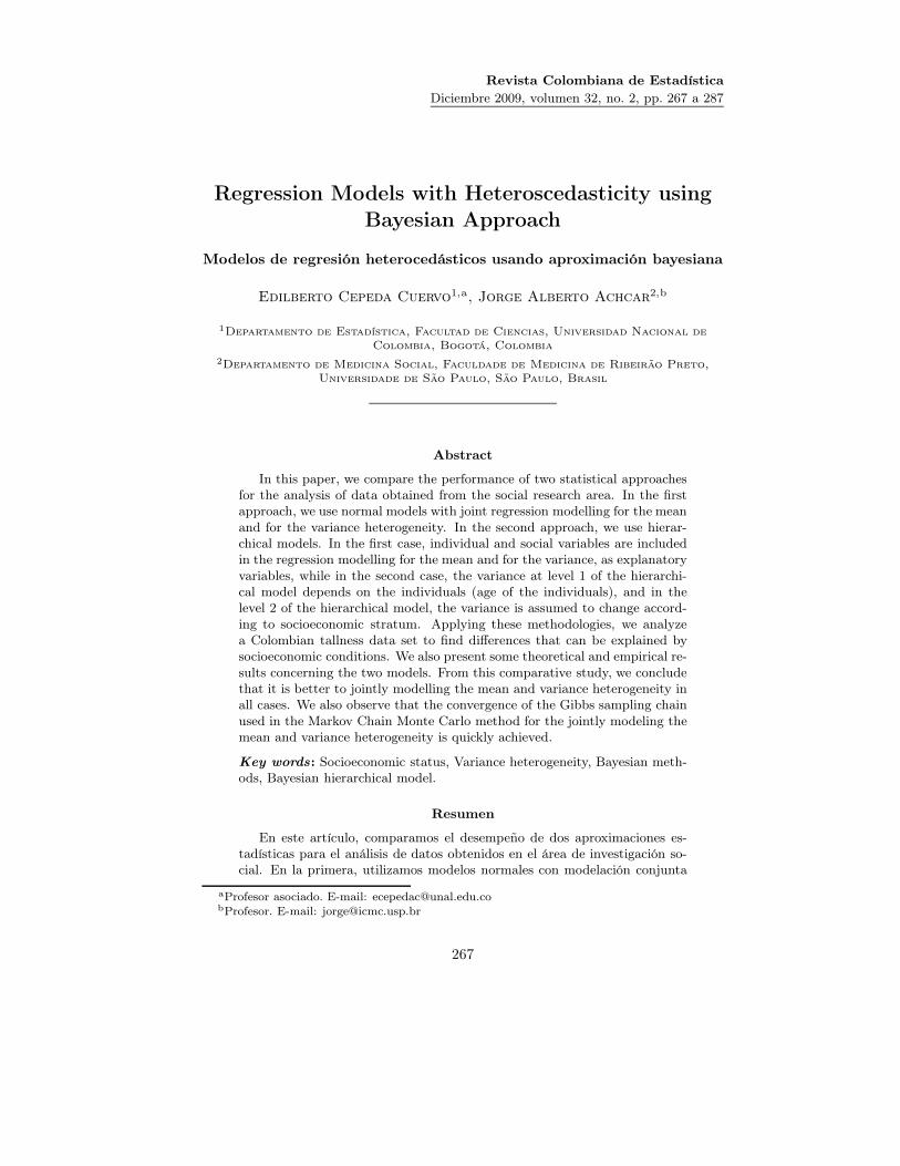
From Figures 5 and 6, we observe that people from lower socioeconomic back-grounds present through time a significantly lower tallness than people from others



0 5 10 15 20

Age (years)

4060

8010

012

014

016

018

0H

eigh

t (cm

)

Figure 5: Mean of tallness of people by socioeconomic level. Continuous line for stratum1, discontinuous line for stratum 2, and dotted line for stratum 3.

socioeconomic strata. People from medium socioeconomic stratum show a signif-icantly lower tallness than people from high socioeconomic stratum, consideringdifferent ages. This fact is easy to understand, since in this case socioeconomic sta-tus has a special relevance on nutrition of people, and people from lower stratumprobably have nutritional deficiencies (see Stein et al. 2004).

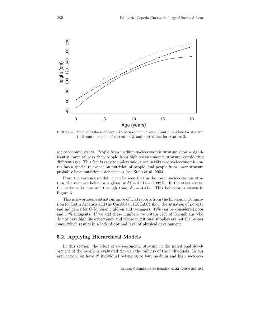
From the variance model, it can be seen that in the lower socioeconomic stra-tum, the variance behavior is given by σ2

i = 3.314 + 0.092Xi. In the other strata,the variance is constant through time, σi = 4.412. This behavior is shown inFigure 6.

This is a worrisome situation, since official reports from the Economic Commis-sion for Latin America and the Caribbean (ECLAC) show the situation of povertyand indigence for Colombian children and teenagers: 45% can be considered poorand 17% indigents. If we add these numbers we obtain 62% of Colombians whodo not have high life expectancy and whose nutritional supplies are not the properones, which results in a lack of optimal level of physical development.

5.2. Applying Hierarchical Models

In this section, the effect of socioeconomic stratum in the nutritional devel-opment of the people is evaluated through the tallness of the individuals. In ourapplication, we have N individual belonging to low, medium and high socioeco-



0 5 10 15 20

Age (years)

4060

8010

012

014

016

018

0H

eigh

t (cm

)

Figure 6: 95% prediction intervals for grown by stratum. Discontinuous line with pointfor stratum 1, continuous line for stratum 2, and discontinuous line for stra-tum 3.

nomic strata. The tallness and the age of each individual were determined anddenoted Yij and tij , respectively, where the subscript ij indicate that the mea-sures belong to the i-th individual belonging to j-th strata. Thus, as it is usual inmultilevel analysis, in the first level, individuals are considered and a regressionmodel (9) is defined for each group.

Yij = β0j + β1jtij + β2jt2ij + εij , εij ∼ N

(0, σ2

)(9)

In this model, βj = (β0j , β1j , β2j) is the parameter vector associated to the j-thstratum, j = 1, 2, 3, and εij is the random error associated in the i-th subject. Inthe second level of the model, the regression coefficient βi is explained by predictedvariables Z, through the model

βkj = γk0Z0j + γk1Z1j + γk2Z2j + ηkj , k = 0, 1, 2 (10)

where Zkj , k = 0, 1, 2, is the set of explanatory variables of level 2, set of indicatorvariables of the stratums k + 1, and ηkj ∼ N

(0, σ2

k

), k = 0, 1, 2. The model is

completed with conjugate prior gamma for the hyperparameters.

Since in this application there is no prior information, we assume normal priordistribution with large variance, that is, approximate non informative prior. Inthis way, we assume normal prior distribution θ ∼ N(0, 10−5I9), where θ is the



vector with components γk′k, k′; k = 0, 1, 2. In this application we assume the priordistributions σ−2

e ∼ G(0.001, .0001) and σ−2k ∼ G(0.001, .0001), k = 0, 1, 2, for the

hyperparameters. The estimates and standard deviations for the parameters ofthe model for the mean of the tallness in each one of the socioeconomic strata aregiven in Table 7. The estimate for the other parameters are: σ2

e = 4.527(3.549),σ2

0 = 5.137(3.438), σ21 = 0.1982(0.09646), σ2

2 = 0.06458(0.004719).

Table 7: Posterior mean estimation on hierarchical models.

γk0 γk1 γk2

k = 0 47.82 (2.371) 61.56 (2.272) 64.89 (2.061)

k = 1 10.25 (0.7447) 8.468 (0.606) 10.39 (0.593)

k = 2 -0.267 (0.045) -0.171 (0.034) -0.267(0.035)

0 5 10 15 20

Age (years)

4060

8010

012

014

016

018

0

Hei

ght (

cm

)

Figure 7: Mean tallness of people by socioeconomic level, hierarchical model. Continu-ous line for lower stratum, discontinuous line for medium stratum and dottedline for high stratum.

In Figure 7, we have the plot of the mean tallness against time for each one ofthe assumed stratum.We can see an agreement between average tallness behaviourshowed in this figure and the behaviour showed in Figure 5, where the analysis wasconducted using joint modelling of the mean and variance heterogeneity. In thisexample, we further observe considerable differences in the BIC values consideringthe different models as we can see in Table 8. From the results of this table, weagain conclude that the model with joint modeling of the mean and of the varianceheterogeneity is better fitted by the data than the hierarchical model.



Table 8: Model comparison.

Model SSE ln L BIC


Hierarchical 28610.283 -3397.753 1183.688

6. Concluding Remarks

From this comparative study for the two proposed models, we conclude that itis better to jointly model the mean and variance heterogeneity, as observed in allexamples, in comparison to the use of hierarchical models. Additionally, conver-gence of the chain used to simulate samples for the posterior distribution of interestis quickly achieved and the model is easily interpretable. The proposed analysiscan be convenient in social applications since these models perfectly capture anyclustering by subgroups that may exist in the data. Other good reason for themodelling of the variance heterogeneity is related to the use of the explanatoryvariables in the regression model, since we can use the same explanatory variablesassumed for the regression model for the mean or other different variables, foreach one of the assumed groups. That is, this analysis also takes into consider-ation one of the most important goals of the multilevel statistical analysis, thatis, it “substantively take into account for causal heterogeneity”. Although there isno statistical differences between intercepts in the growing curves for medium andhight strata, apparently there is an advantage for hight strata through time. Wealso observe that the joint modeling of mean and variance heterogeneity is simplerand easier to interpret.

ˆ

Recibido: marzo de 2009 — Aceptado: noviembre de 2009˜

References

Adair, L. S., Eckhardt, C. L., Gordon-Larsen, P. & Suchindran, C. (2005), ‘TheAssociation Between Diet and Height in the Postinfancy Period Changes withAge and Socioeconomic Status in Filipino Youths’, The Journal of Nutrition

135(9), 2192–2198).

Aitkin, M. (1987), ‘Modelling Variance Heterogeneity in Normal Regression usingGlim’, Applied Statistics 36(4), 332–339.

Bryk, A. & Raudenbush, S. (1992), Hierarchical Linear Models: Applications and

Data Analysis Methods, Sage publications, Inc, Newbury Park, United States.

Cepeda, E. & Gamerman, D. (2001), ‘Bayesian Modeling of Variance Heterogeneityin Normal Regression Models’, Brazilian Journal of Probability and Statistics

14(1), 207–221.

Cepeda, E. & Gamerman, D. (2005), ‘Bayesian Methodology for Modeling Param-eters in the two Parameter Exponential Family’, Revista Estadística 57(168-169), 93–105.



Chumlea, W. C., Guo, S. S., Wholihan, K., Cockram, D., Kuczmarski, R. J.& Johnson, C. L. (1998), ‘Stature Prediction Equations for Elderly Non-Hispanic white, Non-Hispanic Black, and Mexican-American Persons Devel-oped from NHANES III Data’, Journal of the American Dietetic Association

98(2), 137–142.

De Leeuw, J. & Kreft, I. (1986), ‘Random Coefficient Models for Multilevel Anal-ysis’, Journal of Educational Statistics 11, 57–85.

Longford, N. (1993), Random Coefficient Models, Oxford University Press, NewYork, United States.

Prosser, R., Rasbash, J. & Goldstein, H. (1991), ML3. Software for Three-Level

Analysis. User’s Guide for V. 2, GB: Institute of Education, University ofLondon, London, England.

Raudenbush, S. & Bryk, A. (2002), Hierarchical Linear Models: Applications

and Data Analysis Methods, 2 edn, Sage Publications, Inc., Thousand Oaks,United States.

Steenbergen, M. & Bradford, S. (2002), ‘Modeling Multilevel Data Structures’,American Journal of Political Science 46(1), 218–237.

Stein, A. D., Barnhart, H. X., Wang, M., Hoshen, M. B., Ologoudou, K., Ramakr-ishnan, U., Grajeda, R., Ramírez, M. & Martorell, R. (2004), ‘Comparison ofLinear Growth Patterns in the first three Years of Life Across two Generationsin Guatemala’, Pediatrics 113(3), 270–275.

Van Der Leeden, R. (1998), ‘Multilevel Analysis of Repeated Measures Data’,Quality & Quantity. Kluwer Academic Publishers. Netherlands 32, 15–29.

Appendix A.

Hierarchical Models

From the two level hierarchical model definition in Section 3, assuming inde-pendence between n0j and n1j , we have:

Yij | β0j , β1j , Xij , σ2 ∼ N

(β0j + β1jXij , σ

2)

for i = 1, . . . , Nj , j = 1, . . . , J , and

β0j | γ00, γ01, Zj , τ0 ∼ N(γ00 + γ01Zj , τ0)

β1j | γ10, γ11, Zj , τ1 ∼ N(γ10 + γ11Zj , τ1)



Thus the likelihood function is given by,

f`

y | β0, β1, σ2, X

´

=J

Y

j=1

NjY

i=1

1√2πσ2

exp

−1

2σ2(yij − β0j − β1jXij)

2

ff

∝`

σ2´

−1

2

PJj=1

Nj exp

−1

2σ2

JX

j=1

NjX

i=1

(yij − β0j − β1jXij)2

ff

(11)

where β0 = (β01, . . . , β0J )′ and β1 = (β11, . . . , β1J )′.

To apply the Bayesian methodology, we need to specify a prior distributionfunction for θ. For simplicity, we assume independence between parameters, andassign the following prior distributions:

σ2 ∼ IG(a, b) τ20 ∼ IG(co, do)

τ21 ∼ IG(c1, d1) γ00 ∼ N(0, e00)

γ01 ∼ N(0, e01) γ10 ∼ N(0, e10)

γ11 ∼ N(0, e11)

where co, do, c1, d1, e00, e01, e10, e11 are known constants.

With the assumed prior distribution and likelihood function given in (11), theposterior distribution for θ = (γ00, γ01, γ10, γ11, τ0,τ1,β0, β1) is given by

π(θ | y, z, X) ∝ f(y | β0, β1, σ2, X)× π(β0 | γ00, γ01,τ0,z)π(β1 | γ10, γ11,τ1,z)

× π(γ00, γ01, γ10, γ11, σ2, τ0,τ1)

where

π(β0 | γ00, γ01,τ0,z) ∝J∏

j=1

1√2πτ0

exp

{−1

2τ0(β0j − γ00 + γ01Zj)

2

}

∝ (τ0)−

J2 exp

{−1

2τ0

J∑

j=1

Nj∑

i=1

(β0j − γ00 + γ01Zj)2

}

π(β1 | γ10, γ11,τ1,z) ∝J∏

j=1

1√2πτ1

exp

{−1

2τ1(β1j − γ10 + γ11Zj)

2

}

∝ (τ1)−

J2 exp

{−1

2τ1

J∑

j=1

Nj∑

i=1

(β1j − γ10 + γ11Zj)2

}

π(γ00, γ01, γ10, γ11, σ2, τ0,τ1) ∝ exp

− γ200

2e00

ff

exp

− γ201

2e01

ff

exp

− γ210

2e10

ff

exp

− γ211

2e11

ff

× (τ0)−(c0+1)

e−d0/τ0(τ1)

−(c1+1)e−d1/τ1(σ2)−(a+1)

e−b/σ2



Therefore, a joint posterior distribution for θ is given by:

π(θ | y, z, X) ∝ (σ2)−1

2

J∑

j=1

Njexp

{ −1

2σ2

J∑

j=1

Nj∑

i=1


}

× (τ0)−

J2 exp

{−1

2τ0

J∑

j=1

Nj∑

i=1

(β0j − γ00 + γ01Zj)2

}

× (τ1)−

J2 exp

{−1

2τ1

J∑

j=1

Nj∑

i=1

(β1j − γ10 + γ11Zj)2

}

× exp

{− γ2

00

2e00

}exp

{− γ2

01

2e01

}exp

{− γ2

10

2e10

}exp

{− γ2

11

2e11

}

× (τ0)−(c0+1)e−d0/τ0(τ1)

−(c1+1)e−d1/τ1(σ2)−(a+1)e−b/σ2

where σ2 > 0, τ0, > 0, τ1, > 0, γ00, γ01, γ10, γ11, εR and β1j , β1jεR; j = 1, . . . , J .The parameter vector θ = (γ00, γ01, γ10, γ11, σ

2, τ0,τ1,β01, . . . , β01, β11, . . . , β1J) has25+7 components.

Thus, the conditional posterior distribution is given by

σ2 | θ(σ2), y, z, X ∼ IG

{a +

1

2

J∑

j=1

Nj ; b +1

2

J∑

j=1

Nj∑

i=1

(yij − β0j − βijXij)2

}

τ0 | θ(τ0), y, z, X ∼ IG

{c0 +

J

2; d0 +

1

2

J∑

j=1

(β0j − γ00 − γ01Zj)2

}

τ1 | θ(τ0), y, z, X ∼ IG

{c1 +

J

2; d1 +

1

2

J∑

j=1

(β1j − γ01 − γ11Zj)2

}

γ00 | θ(j00), y, z, X ∼ N

(e200

∑Jj=1 µ00j

τ0 + Je200

;τ0e

200

τ0 + Je200

)

γ10 | θ(j10), y, z, X ∼ N

(e210

∑Jj=1 µ10j

τ1 + Je210

;τ1e

210

τ1 + Je210

)

γ01 | θ(j01), y, z, X ∼ N

(e201

∑Jj=1 zjµ01j

τ0 + e210

∑Jj=1 z2

j

;τ0e

210

τ0 + e210

∑Jj=1 z2

j

)

γ11 | θ(j11), y, z, X ∼ N

(e211

∑Jj=1 zjµ11j

τ1 + e210

∑Jj=1 z2

j

;τ1e

211

τ1 + e211

∑Jj=1 z2

j

)

where µ00j=β0j − γ01Zj ; j = 1, . . . , J ; µ10j=β1j − γ11Zj ; j = 1, . . . , J ; µ01j=β0j −γ00; j = 1, . . . , J ; µ11j=β1j − γ10; j = 1, . . . , J .



For β′s, given that

π(β0j | θ(β0j), y, z, X) ∝ exp

{− 1

2τ0(β0j − γ00 − γ01Zj)

2

}

× exp

{ −1

2σ2

Nj∑

i=1


}

then all posterior conditional distributions for β0j are given by:

β0j | θ(β0j), y, z, X ∼ N

(σ2(j00 + j01Zj) + τ0

∑Nj

i=1 a0ij

σ2 + τ0Nj;

σ2τ0

σ2 + τ0Nj

)

where a0ij = yij − β1jXij ; j = 1, . . . , J .

In the same way, given that

π(β1j | θ(β1j), y, z, X) ∝ exp

{− 1

2τ1(β1j − γ10 − γ11Zj)

2

}

× exp

{ −1

2σ2

Nj∑

i=1


}

all posterior conditional distributions for β0j are given by

β1j | θ(β1j),y,z,X ∼ N

(σ2(j10 + j11Zj) + τ1

∑Nj

i=1 a1ij

σ2 + τ01

∑Nj

i=1 Xij

;σ2τ1

σ2 + τ1Nj

)

where a1ij = yij − β0j ; j = 1, . . . , J .


Documents

Regression Models with Heteroscedasticity using Bayesian ... · Revista Colombiana de Estadística Diciembre 2009, volumen 32, no. 2, pp. 267 a 287 Regression Models with Heteroscedasticity