Embed Size (px)
Citation preview

Foundations and TrendsR© inMachine LearningVol. 5, No. 1 (2012) 1–122c© 2012 S. Bubeck and N. Cesa-BianchiDOI: 10.1561/2200000024
Regret Analysis of Stochastic andNonstochastic Multi-armed
Bandit Problems
By Sebastien Bubeck and Nicolo Cesa-Bianchi
Contents
1 Introduction 2
2 Stochastic Bandits: Fundamental Results 9
2.1 Optimism in Face of Uncertainty 102.2 Upper Confidence Bound (UCB) Strategies 112.3 Lower Bound 132.4 Refinements and Bibliographic Remarks 17
3 Adversarial Bandits: Fundamental Results 22
3.1 Pseudo-regret Bounds 233.2 High Probability and Expected Regret Bounds 283.3 Lower Bound 333.4 Refinements and Bibliographic Remarks 37
4 Contextual Bandits 43
4.1 Bandits with Side Information 444.2 The Expert Case 454.3 Stochastic Contextual Bandits 534.4 The Multiclass Case 564.5 Bibliographic Remarks 62
5 Linear Bandits 64
5.1 Exp2 (Expanded Exp) with John’s Exploration 655.2 Online Mirror Descent (OMD) 695.3 Online Stochastic Mirror Descent (OSMD) 745.4 Online Combinatorial Optimization 765.5 Improved Regret Bounds for Bandit Feedback 815.6 Refinements and Bibliographic Remarks 84
6 Nonlinear Bandits 88
6.1 Two-Point Bandit Feedback 896.2 One-Point Bandit Feedback 946.3 Nonlinear Stochastic Bandits 966.4 Bibliographic Remarks 101
7 Variants 103
7.1 Markov Decision Processes,Restless and Sleeping Bandits 104
7.2 Pure Exploration Problems 1057.3 Dueling Bandits 1077.4 Discovery with Probabilistic Expert Advice 1077.5 Many-Armed Bandits 1087.6 Truthful Bandits 1097.7 Concluding Remarks 109
Acknowledgments 111
References 112

Foundations and TrendsR© inMachine LearningVol. 5, No. 1 (2012) 1–122c© 2012 S. Bubeck and N. Cesa-BianchiDOI: 10.1561/2200000024
Regret Analysis of Stochastic andNonstochastic Multi-armed
Bandit Problems
Sebastien Bubeck1 and Nicolo Cesa-Bianchi2
1 Department of Operations Research and Financial Engineering, PrincetonUniversity, Princeton, NJ 08544, USA, [email protected]
2 Dipartimento di Informatica, Universita degli Studi di Milano, Milano20135, Italy, [email protected]
Abstract
Multi-armed bandit problems are the most basic examples of sequentialdecision problems with an exploration–exploitation trade-off. This isthe balance between staying with the option that gave highest payoffsin the past and exploring new options that might give higher payoffsin the future. Although the study of bandit problems dates back tothe 1930s, exploration–exploitation trade-offs arise in several modernapplications, such as ad placement, website optimization, and packetrouting. Mathematically, a multi-armed bandit is defined by the payoffprocess associated with each option. In this monograph, we focus on twoextreme cases in which the analysis of regret is particularly simple andelegant: i.i.d. payoffs and adversarial payoffs. Besides the basic settingof finitely many actions, we also analyze some of the most importantvariants and extensions, such as the contextual bandit model.

1Introduction
A multi-armed bandit problem (or, simply, a bandit problem) is asequential allocation problem defined by a set of actions. At each timestep, a unit resource is allocated to an action and some observablepayoff is obtained. The goal is to maximize the total payoff obtainedin a sequence of allocations. The name bandit refers to the colloquialterm for a slot machine (“one-armed bandit” in American slang). In acasino, a sequential allocation problem is obtained when the player isfacing many slot machines at once (a “multi-armed bandit”) and mustrepeatedly choose where to insert the next coin.
Bandit problems are basic instances of sequential decision makingwith limited information and naturally address the fundamental trade-off between exploration and exploitation in sequential experiments.Indeed, the player must balance the exploitation of actions that didwell in the past and the exploration of actions that might give higherpayoffs in the future.
Although the original motivation of Thompson [162] for studyingbandit problems came from clinical trials (when different treatmentsare available for a certain disease and one must decide which treat-ment to use on the next patient), modern technologies have created
2
3
many opportunities for new applications, and bandit problems nowplay an important role in several industrial domains. In particular,online services are natural targets for bandit algorithms, because thereone can benefit from adapting the service to the individual sequence ofrequests. We now describe a few concrete examples in various domains.
Ad placement is the problem of deciding which advertisement todisplay on the web page delivered to the next visitor of a website.Similarly, website optimization deals with the problem of sequentiallychoosing design elements (font, images, layout) for the web page. Herethe payoff is associated with visitor’s actions, e.g., clickthroughs orother desired behaviors. Of course there are important differences withthe basic bandit problem: in ad placement the pool of available ads(bandit arms) may change over time, and there might be a limit on thenumber of times each ad could be displayed.
In source routing a sequence of packets must be routed from a sourcehost to a destination host in a given network, and the protocol allows tochoose a specific source-destination path for each packet to be sent. The(negative) payoff is the time it takes to deliver a packet, and dependsadditively on the congestion of the edges in the chosen path.
In computer game-playing, each move is chosen by simulatingand evaluating many possible game continuations after the move.Algorithms for bandits (more specifically, for a tree-based version of thebandit problem) can be used to explore more efficiently the huge tree ofgame continuations by focusing on the most promising subtrees. Thisidea has been successfully implemented in the MoGo player of Gellyet al. [85], which plays Go at world-class level. MoGo is based on theUCT strategy for hierarchical bandits of Kocsis and Szepesvari [123],which in turn is derived from the UCB bandit algorithm — seeSection 2.
There are three fundamental formalizations of the bandit problemdepending on the assumed nature of the reward process: stochastic,adversarial, and Markovian. Three distinct playing strategies have beenshown to effectively address each specific bandit model: the UCB algo-rithm in the stochastic case, the Exp3 randomized algorithm in theadversarial case, and the so-called Gittins indices in the Markoviancase. In this monograph, we focus on stochastic and adversarial bandits,
4 Introduction
and refer the reader to the monograph by Mahajan and Teneketzis [130]or to the recent monograph by Gittins et al. [86] for an extensive anal-ysis of Markovian bandits.
In order to analyze the behavior of a player or forecaster (i.e.,the agent implementing a bandit strategy), we may compare its per-formance with that of an optimal strategy that, for any horizon ofn time steps, consistently plays the arm that is best in the first nsteps. In other terms, we may study the regret of the forecaster fornot playing always optimally. More specifically, given K ≥ 2 arms andsequences Xi,1,Xi,2, . . . of unknown rewards associated with each armi = 1, . . . ,K, we study forecasters that at each time step t = 1,2, . . .select an arm It and receive the associated reward XIt,t. The regretafter n plays I1, . . . , In is defined by
Rn = maxi=1,...,K
n∑t=1
Xi,t −n∑t=1
XIt,t. (1.1)
If the time horizon is not known in advance we say that the forecasteris anytime.
In general, both rewards Xi,t and forecaster’s choices It might bestochastic. This allows to distinguish between the two following notionsof averaged regret: the expected regret
ERn = E
[max
i=1,...,K
n∑t=1
Xi,t −n∑t=1
XIt,t
](1.2)
and the pseudo-regret
Rn = maxi=1,...,K
E
[n∑t=1
Xi,t −n∑t=1
XIt,t
]. (1.3)
In both definitions, the expectation is taken with respect to the randomdraw of both rewards and forecaster’s actions. Note that pseudo-regretis a weaker notion of regret, since one competes against the action whichis optimal only in expectation. The expected regret, instead, is theexpectation of the regret with respect to the action which is optimal onthe sequence of reward realizations. More formally one has Rn ≤ ERn.
In the original formalization of Robbins [146], which builds on thework of Wald [164] — see also Arrow et al. [16], each arm i = 1, . . . ,K

5
corresponds to an unknown probability distribution νi on [0,1], andrewardsXi,t are independent draws from the distribution νi correspond-ing to the selected arm.
The stochastic bandit problem
Known parameters: number of arms K and (possibly) number of rounds n ≥ K.Unknown parameters: K probability distributions ν1, . . . ,νK on [0,1].
For each round t = 1,2, . . .
(1) the forecaster chooses It ∈ 1, . . . ,K;(2) given It, the environment draws the reward XIt,t ∼ νIt indepen-
dently from the past and reveals it to the forecaster.
For i = 1, . . . ,K we denote by µi the mean of νi (mean reward of arm i).Let
µ∗ = maxi=1,...,K
µi and i∗ ∈ argmaxi=1,...,K
µi.
In the stochastic setting, it is easy to see that the pseudo-regret can bewritten as
Rn = nµ∗ −n∑t=1
E[µIt ]. (1.4)
The analysis of the stochastic bandit model was pioneered in the sem-inal paper of Lai and Robbins [125], who introduced the techniqueof upper confidence bounds for the asymptotic analysis of regret. InSection 2 we describe this technique using the simpler formulation ofAgrawal [9], which naturally lends itself to a finite-time analysis.
In parallel to the research on stochastic bandits, a game-theoreticformulation of the trade-off between exploration and exploitationhas been independently investigated, although for quite some timethis alternative formulation was not recognized as an instance ofthe multi-armed bandit problem. In order to motivate these game-theoretic bandits, consider again the initial example of gambling onslot machines. We now assume that we are in a rigged casino, wherefor each slot machine i = 1, . . . ,K and time step t ≥ 1 the owner setsthe gain Xi,t to some arbitrary (and possibly maliciously chosen) value

6 Introduction
gi,t ∈ [0,1]. Note that it is not in the interest of the owner to simply setall the gains to zero (otherwise, no gamblers would go to that casino).Now recall that a forecaster selects sequentially one arm It ∈ 1, . . . ,Kat each time step t = 1,2, . . . and observes (and earns) the gain gIt,t. Isit still possible to minimize regret in such a setting?
Following a standard terminology, we call adversary, or opponent,the mechanism setting the sequence of gains for each arm. If this mecha-nism is independent of the forecaster’s actions, then we call it an obliv-ious adversary. In general, however, the adversary may adapt to theforecaster’s past behavior, in which case we speak of a nonobliviousadversary. For instance, in the rigged casino the owner may observethe way a gambler plays in order to design even more evil sequencesof gains. Clearly, the distinction between oblivious and nonobliviousadversary is only meaningful when the player is randomized (if theplayer is deterministic, then the adversary can pick a bad sequence ofgains right at the beginning of the game by simulating the player’sfuture actions). Note, however, that in the presence of a nonobliviousadversary the interpretation of regret is ambiguous. Indeed, in this casethe assignment of gains gi,t to arms i = 1, . . . ,K made by the adver-sary at each step t is allowed to depend on the player’s past random-ized actions I1, . . . , It−1. In other words, gi,t = gi,t(I1, . . . , It−1) for eachi and t. Now, the regret compares the player’s cumulative gain to thatobtained by playing the single best arm for the first n rounds. However,had the player consistently chosen the same arm i in each round, namelyIt = i for t = 1, . . . ,n, the adversarial gains gi,t(I1, . . . , It−1) wouldhave been possibly different than those actually experienced by theplayer.
The study of nonoblivious regret is mainly motivated by the con-nection between regret minimization and equilibria in games — see,e.g., [24, Section 9]. Here we just observe that game-theoretic equilibriaare indeed defined similarly to regret: in equilibrium, the player has nSoincentive to behave differently, provided the opponent does not reactto changes in the player’s behavior. Interestingly, regret minimizationhas been also studied against reactive opponents, see for instance theworks of Pucci de Farias and Megiddo [144] and Arora et al. [14].
7
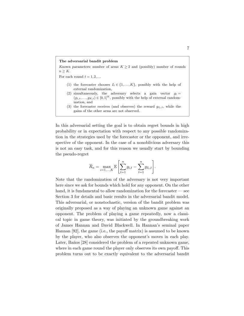
The adversarial bandit problem
Known parameters: number of arms K ≥ 2 and (possibly) number of roundsn ≥ K.
For each round t = 1,2, . . .
(1) the forecaster chooses It ∈ 1, . . . ,K, possibly with the help ofexternal randomization,
(2) simultaneously, the adversary selects a gain vector gt =(g1,t, . . . ,gK,t) ∈ [0,1]K , possibly with the help of external random-ization, and
(3) the forecaster receives (and observes) the reward gIt,t, while thegains of the other arms are not observed.
In this adversarial setting the goal is to obtain regret bounds in highprobability or in expectation with respect to any possible randomiza-tion in the strategies used by the forecaster or the opponent, and irre-spective of the opponent. In the case of a nonoblivious adversary thisis not an easy task, and for this reason we usually start by boundingthe pseudo-regret
Rn = maxi=1,...,K
E
[n∑t=1
gi,t −n∑t=1
gIt,t
].
Note that the randomization of the adversary is not very importanthere since we ask for bounds which hold for any opponent. On the otherhand, it is fundamental to allow randomization for the forecaster — seeSection 3 for details and basic results in the adversarial bandit model.This adversarial, or nonstochastic, version of the bandit problem wasoriginally proposed as a way of playing an unknown game against anopponent. The problem of playing a game repeatedly, now a classi-cal topic in game theory, was initiated by the groundbreaking workof James Hannan and David Blackwell. In Hannan’s seminal paperHannan [92], the game (i.e., the payoff matrix) is assumed to be knownby the player, who also observes the opponent’s moves in each play.Later, Banos [28] considered the problem of a repeated unknown game,where in each game round the player only observes its own payoff. Thisproblem turns out to be exactly equivalent to the adversarial bandit

8 Introduction
problem with a nonoblivious adversary. Simpler strategies for playingunknown games were more recently proposed by Foster and Vohra [81]and Hart and Mas-Colell [93, 94]. Approximately at the same time, theproblem was re-discovered in computer science by Auer et al. [24]. Itwas them who made apparent the connection to stochastic bandits bycoining the term nonstochastic multi-armed bandit problem.
The third fundamental model of multi-armed bandits assumes thatthe reward processes are neither i.i.d. (like in stochastic bandits) noradversarial. More precisely, arms are associated with K Markov pro-cesses, each with its own state space. Each time an arm i is chosen instate s, a stochastic reward is drawn from a probability distribution νi,s,and the state of the reward process for arm i changes in a Markovianfashion, based on an underlying stochastic transition matrix Mi. Bothreward and new state are revealed to the player. On the other hand,the state of arms that are not chosen remains unchanged. Going backto our initial interpretation of bandits as sequential resource allocationprocesses, here we may think of K competing projects that are sequen-tially allocated a unit resource of work. However, unlike the previousbandit models, in this case the state of a project that gets the resourcemay change. Moreover, the underlying stochastic transition matricesMi are typically assumed to be known, thus the optimal policy can becomputed via dynamic programming and the problem is essentially ofcomputational nature. The seminal result of Gittins [87] provides anoptimal greedy policy which can be computed efficiently.
A notable special case of Markovian bandits is that of Bayesianbandits. These are parametric stochastic bandits, where the parame-ters of the reward distributions are assumed to be drawn from knownpriors, and the regret is computed by also averaging over the drawof parameters from the prior. The Markovian state change associatedwith the selection of an arm corresponds here to updating the posteriordistribution of rewards for that arm after observing a new reward.
Markovian bandits are a standard model in the areas of OperationsResearch and Economics. However, the techniques used in their analysisare significantly different from those used to analyze stochastic andadversarial bandits. For this reason, in this monograph we do not coverMarkovian bandits and their many variants.

2Stochastic Bandits: Fundamental Results
We start by recalling the basic definitions for the stochastic banditproblem. Each arm i ∈ 1, . . . ,K corresponds to an unknown probabil-ity distribution νi. At each time step t = 1,2, . . . , the forecaster selectssome arm It ∈ 1, . . . ,K and receives a reward XIt,t drawn from νIt(independently from the past). Denote by µi the mean of arm i anddefine
µ∗ = maxi=1,...,K
µi and i∗ ∈ argmaxi=1,...,K
µi.
We focus here on the pseudo-regret, which is defined as
Rn = nµ∗ − E
n∑t=1
µIt . (2.1)
We choose the pseudo-regret as our main quantity of interest becausein a stochastic framework it is more natural to compete against theoptimal action in expectation, rather than the optimal action on thesequence of realized rewards (as in the definition of the plain regretin Equation (1.1)). Furthermore, because of the order of magnitudeof typical random fluctuations, in general one cannot hope to prove abound on the expected regret in Equation (1.2) better than Θ(
√n).
9
10 Stochastic Bandits: Fundamental Results
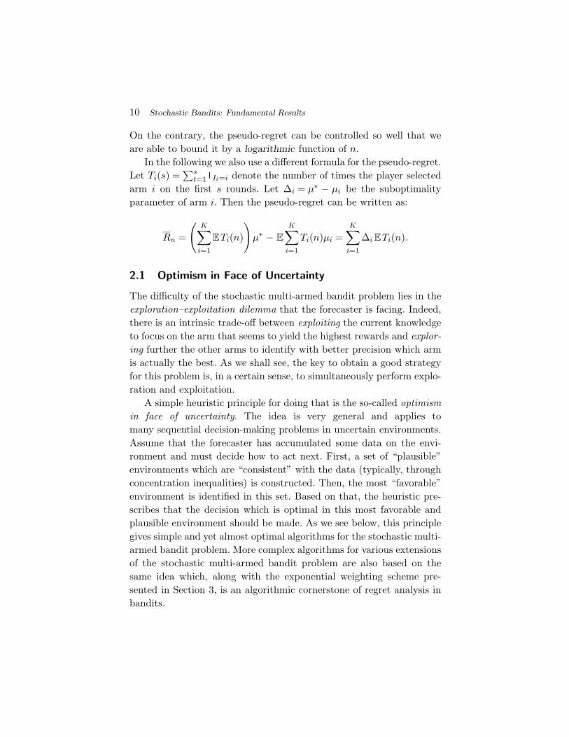
On the contrary, the pseudo-regret can be controlled so well that weare able to bound it by a logarithmic function of n.
In the following we also use a different formula for the pseudo-regret.Let Ti(s) =
∑st=1 It=i denote the number of times the player selected
arm i on the first s rounds. Let ∆i = µ∗ − µi be the suboptimalityparameter of arm i. Then the pseudo-regret can be written as:
Rn =
(K∑i=1
ETi(n)
)µ∗ − E
K∑i=1
Ti(n)µi =K∑i=1
∆iETi(n).
2.1 Optimism in Face of Uncertainty
The difficulty of the stochastic multi-armed bandit problem lies in theexploration–exploitation dilemma that the forecaster is facing. Indeed,there is an intrinsic trade-off between exploiting the current knowledgeto focus on the arm that seems to yield the highest rewards and explor-ing further the other arms to identify with better precision which armis actually the best. As we shall see, the key to obtain a good strategyfor this problem is, in a certain sense, to simultaneously perform explo-ration and exploitation.
A simple heuristic principle for doing that is the so-called optimismin face of uncertainty. The idea is very general and applies tomany sequential decision-making problems in uncertain environments.Assume that the forecaster has accumulated some data on the envi-ronment and must decide how to act next. First, a set of “plausible”environments which are “consistent” with the data (typically, throughconcentration inequalities) is constructed. Then, the most “favorable”environment is identified in this set. Based on that, the heuristic pre-scribes that the decision which is optimal in this most favorable andplausible environment should be made. As we see below, this principlegives simple and yet almost optimal algorithms for the stochastic multi-armed bandit problem. More complex algorithms for various extensionsof the stochastic multi-armed bandit problem are also based on thesame idea which, along with the exponential weighting scheme pre-sented in Section 3, is an algorithmic cornerstone of regret analysis inbandits.
2.2 Upper Confidence Bound (UCB) Strategies 11
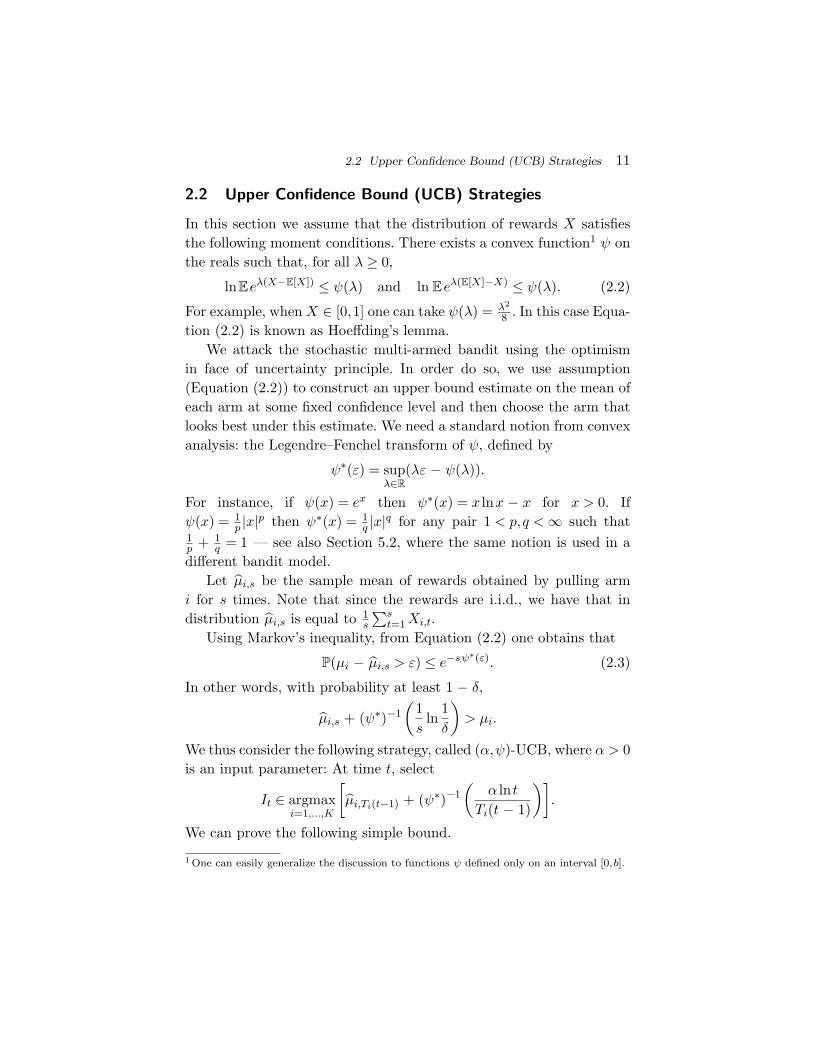
2.2 Upper Confidence Bound (UCB) Strategies
In this section we assume that the distribution of rewards X satisfiesthe following moment conditions. There exists a convex function1 ψ onthe reals such that, for all λ ≥ 0,
lnEeλ(X−E[X]) ≤ ψ(λ) and ln Eeλ(E[X]−X) ≤ ψ(λ). (2.2)
For example, whenX ∈ [0,1] one can take ψ(λ) = λ2
8 . In this case Equa-tion (2.2) is known as Hoeffding’s lemma.
We attack the stochastic multi-armed bandit using the optimismin face of uncertainty principle. In order do so, we use assumption(Equation (2.2)) to construct an upper bound estimate on the mean ofeach arm at some fixed confidence level and then choose the arm thatlooks best under this estimate. We need a standard notion from convexanalysis: the Legendre–Fenchel transform of ψ, defined by
ψ∗(ε) = supλ∈R
(λε − ψ(λ)).
For instance, if ψ(x) = ex then ψ∗(x) = x lnx − x for x > 0. Ifψ(x) = 1
p |x|p then ψ∗(x) = 1q |x|q for any pair 1 < p,q <∞ such that
1p + 1
q = 1 — see also Section 5.2, where the same notion is used in adifferent bandit model.
Let µi,s be the sample mean of rewards obtained by pulling armi for s times. Note that since the rewards are i.i.d., we have that indistribution µi,s is equal to 1
s
∑st=1Xi,t.
Using Markov’s inequality, from Equation (2.2) one obtains that
P(µi − µi,s > ε) ≤ e−sψ∗(ε). (2.3)
In other words, with probability at least 1 − δ,µi,s + (ψ∗)−1
(1s
ln1δ
)> µi.
We thus consider the following strategy, called (α,ψ)-UCB, where α > 0is an input parameter: At time t, select
It ∈ argmaxi=1,...,K
[µi,Ti(t−1) + (ψ∗)−1
(α ln t
Ti(t − 1)
)].
We can prove the following simple bound.
1 One can easily generalize the discussion to functions ψ defined only on an interval [0, b].

12 Stochastic Bandits: Fundamental Results
Theorem 2.1 (Pseudo-regret of (α,ψ)-UCB). Assume that thereward distributions satisfy Equation (2.2). Then (α,ψ)-UCB withα > 2 satisfies
Rn ≤∑
i :∆i>0
(α∆i
ψ∗(∆i/2)lnn +
α
α − 2
).
In case of [0,1]-valued random variables, taking ψ(λ) = λ2
8 in Equa-tion (2.2) — the Hoeffding’s Lemma — gives ψ∗(ε) = 2ε2, which inturns gives the following pseudo-regret bound
Rn ≤∑i:∆i>0
(2α∆i
lnn +α
α − 2
). (2.4)
In this important special case of bounded random variables we refer to(α,ψ)-UCB simply as α-UCB.
Proof. First note that if It = i, then at least one of the three followingequations must be true:
µi∗,Ti∗ (t−1) + (ψ∗)−1(
α ln tTi∗(t − 1)
)≤ µ∗ (2.5)
µi,Ti(t−1) > µi + (ψ∗)−1(
α ln tTi(t − 1)
)(2.6)
Ti(t − 1) <α lnn
ψ∗(∆i/2). (2.7)
Indeed, assume that the three equations are all false, then we have:
µi∗,Ti∗ (t−1) + (ψ∗)−1(
α ln tTi∗(t − 1)
)> µ∗
= µi + ∆i
≥ µi + 2(ψ∗)−1(
α ln tTi(t − 1)
)≥ µi,Ti(t−1) + (ψ∗)−1
(α ln t
Ti(t − 1)
)
2.3 Lower Bound 13
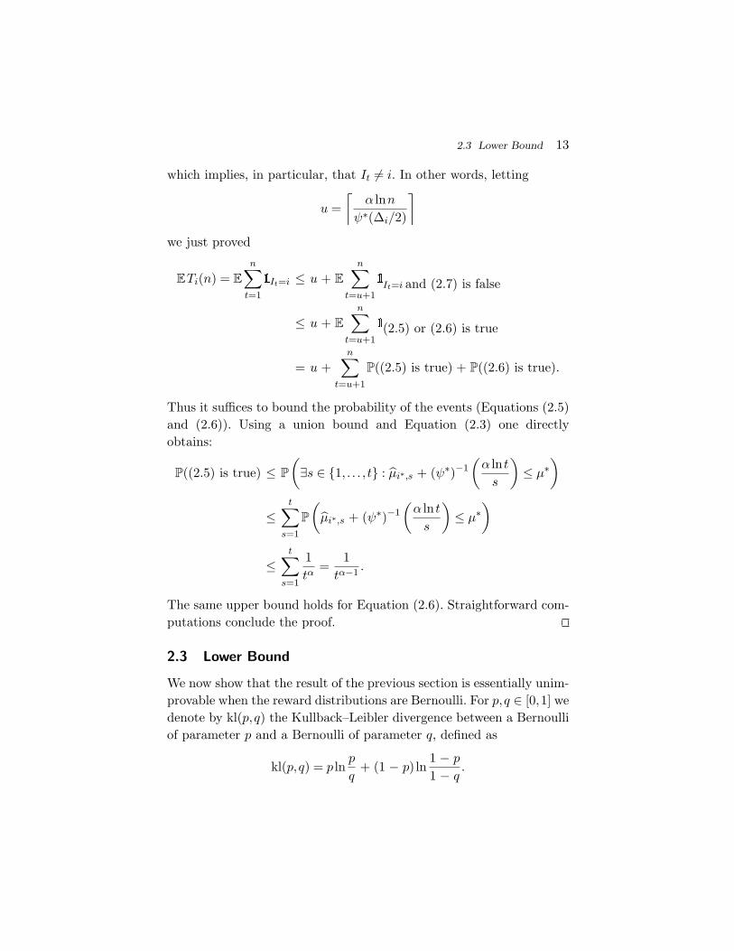
which implies, in particular, that It = i. In other words, letting
u =⌈
α lnnψ∗(∆i/2)
⌉we just proved
ETi(n) = E
n∑t=1
It=i ≤ u + E
n∑t=u+1
It=i and (2.7) is false
≤ u + E
n∑t=u+1
(2.5) or (2.6) is true
= u +n∑
t=u+1
P((2.5) is true) + P((2.6) is true).
Thus it suffices to bound the probability of the events (Equations (2.5)and (2.6)). Using a union bound and Equation (2.3) one directlyobtains:
P((2.5) is true) ≤ P
(∃s ∈ 1, . . . , t : µi∗,s + (ψ∗)−1
(α ln ts
)≤ µ∗)
≤t∑
s=1
P
(µi∗,s + (ψ∗)−1
(α ln ts
)≤ µ∗)
≤t∑
s=1
1tα
=1
tα−1 .
The same upper bound holds for Equation (2.6). Straightforward com-putations conclude the proof.
2.3 Lower Bound
We now show that the result of the previous section is essentially unim-provable when the reward distributions are Bernoulli. For p,q ∈ [0,1] wedenote by kl(p,q) the Kullback–Leibler divergence between a Bernoulliof parameter p and a Bernoulli of parameter q, defined as
kl(p,q) = p lnp
q+ (1 − p) ln
1 − p1 − q .
14 Stochastic Bandits: Fundamental Results
Theorem 2.2 (Distribution-dependent lower bound). Considera strategy that satisfies ETi(n) = o(na) for any set of Bernoulli rewarddistributions, any arm i with ∆i > 0, and any a > 0. Then, for any setof Bernoulli reward distributions the following holds
liminfn→+∞
Rnlnn≥∑
i :∆i>0
∆i
kl(µi,µ∗).
In order to compare this result with Equation (2.4) we use the fol-lowing standard inequalities (the left-hand side follows from Pinsker’sinequality and the right-hand side simply uses lnx ≤ x − 1),
2(p − q)2 ≤ kl(p,q) ≤ (p − q)2q(1 − q) . (2.8)
Proof. The proof is organized in three steps. For simplicity, we onlyconsider the case of two arms.
First step: Notations
Without loss of generality assume that arm 1 is optimal and arm 2is suboptimal, that is, µ2 < µ1 < 1. Let ε > 0. Since x → kl(µ2,x) iscontinuous one can find µ′
2 ∈ (µ1,1) such that
kl(µ2,µ′2) ≤ (1 + ε)kl(µ2,µ1). (2.9)
We use the notation E′,P′ when we integrate with respect to the mod-
ified bandit where the parameter of arm 2 is replaced by µ′2. We want
to compare the behavior of the forecaster on the initial and modifiedbandits. In particular, we prove that with a big enough probability theforecaster cannot distinguish between the two problems. Then, usingthe fact that we have a good forecaster by hypothesis, we know thatthe algorithm does not make too many mistakes on the modified ban-dit where arm 2 is optimal. In other words, we have a lower bound onthe number of times the optimal arm is played. This reasoning impliesa lower bound on the number of times arm 2 is played in the initialproblem.

2.3 Lower Bound 15
We now slightly change the notation for rewards and denote byX2,1, . . . ,X2,n the sequence of random variables obtained when pullingarm 2 for n times (that is, X2,s is the reward obtained from the s-thpull). For s ∈ 1, . . . ,n, let
kls =s∑t=1
lnµ2X2,t + (1 − µ2)(1 − X2,t)µ′
2X2,t + (1 − µ′2)(1 − X2,t)
.
Note that, with respect to the initial bandit, klT2(n) is the (nonre-normalized) empirical estimate of kl(µ2,µ
′2) at time n, since in that case
the process (X2,s) is i.i.d. from a Bernoulli of parameter µ2. Anotherimportant property is the following: for any event A in the σ-algebragenerated by X2,1, . . . ,X2,n the following change-of-measure identityholds:
P′(A) = E[ A exp(−klT2(n))]. (2.10)
In order to link the behavior of the forecaster on the initial and modifiedbandits we introduce the event
Cn =T2(n) <
1 − εkl(µ2,µ′
2)ln(n) and klT2(n) ≤
(1 − ε
2
)ln(n)
.
(2.11)
Second step: P(Cn) = o(1)
By Equations (2.10) and (2.11) one has
P′(Cn) = E Cn exp(−klT2(n)) ≥ e−(1−ε/2) ln(n)
P(Cn).
Introduce the shorthand
fn =1 − ε
kl(µ2,µ′2)
ln(n).
Using again Equation (2.11) and Markov’s inequality, the above implies
P(Cn) ≤ n(1−ε/2)P
′(Cn) ≤ n(1−ε/2)P
′(T2(n) < fn)
≤ n(1−ε/2) E′[n − T2(n)]n − fn .

16 Stochastic Bandits: Fundamental Results
Now note that in the modified bandit arm 2 is the unique optimal arm.Hence the assumption that for any bandit, any suboptimal arm i, andany a > 0, the strategy satisfies ETi(n) = o(na), implies that
P(Cn) ≤ n(1−ε/2) E′[n − T2(n)]n − fn = o(1).
Third step: P(T2(n) < fn) = o(1).
Observe that
P(Cn) ≥ P
(T2(n) < fn and max
s≤fn
kls ≤(1 − ε
2
)ln(n)
)= P
(T2(n) < fn and
kl(µ2,µ′2)
(1 − ε) ln(n)
×maxs≤fn
kls ≤ 1 − ε/21 − ε kl(µ2,µ
′2)). (2.12)
Now we use the maximal version of the strong law of large numbers: forany sequence (Xt) of independent real random variables with positivemean µ > 0,
limn→∞
1n
n∑t=1
Xt = µ a.s. implies limn→∞
1n
maxs=1,...,n
s∑t=1
Xt = µ a.s.
See, e.g., [43, Lemma 10.5].Since kl(µ2,µ
′2) > 0 and 1−ε/2
1−ε > 1, we deduce that
limn→∞P
(kl(µ2,µ
′2)
(1 − ε) ln(n)× max
s≤fn
kls ≤ 1 − ε/21 − ε kl(µ2,µ
′2))
= 1.
Thus, by the result of the second step and Equation (2.12), we get
P(T2(n) < fn) = o(1).
Now recalling that fn = 1−εkl(µ2,µ′
2) ln(n), and using Equation (2.9), weobtain
ET2(n) ≥ (1 + o(1))1 − ε1 + ε
ln(n)kl(µ2,µ1)
which concludes the proof.
2.4 Refinements and Bibliographic Remarks 17
2.4 Refinements and Bibliographic Remarks
The UCB strategy presented in Section 2.2 was introduced by Aueret al. [23] for bounded random variables. Theorem 2.2 is extractedfrom Lai and Robbins [125]. Note that in this last paper the result ismore general than ours, which is restricted to Bernoulli distributions.Although Burnetas and Katehakis [56] prove an even more generallower bound, Theorem 2.2 and the UCB regret bound provide a rea-sonably complete solution to the problem. We now discuss some of thepossible refinements. In the following, we restrict our attention to thecase of bounded rewards (except in Section 2.4.7).
2.4.1 Improved Constants
The regret bound proof for UCB can be improved in two ways. First,the union bound over the different time steps can be replaced by a“peeling” argument. This allows to show a logarithmic regret for anyα > 1, whereas the proof of Section 2.2 requires α > 2 — see [43,Section 2.2] for more details. A second improvement, proposed byGarivier and Cappe [83], is to use a more subtle set of conditions thanEquations (2.5)–(2.7). In fact, the authors take both improvementsinto account, and show that α-UCB has a regret of order α
2 lnn for anyα > 1. In the limit when α tends to 1, this constant is unimprovable inlight of Theorem 2.2 and Equation (2.8).
2.4.2 Second-Order Bounds
Although α-UCB is essentially optimal, the gap between Equation (2.4)and Theorem 2.2 can be important if kl(µi∗ ,µi) is significantly largerthan ∆2
i . Several improvements have been proposed toward closing thisgap. In particular, the UCB-V algorithm of Audibert et al. [21] takesinto account the variance of the distributions and replaces Hoeffding’sinequality by Bernstein’s inequality in the derivation of UCB. A pre-vious algorithm with similar ideas was developed by Auer et al. [23]without theoretical guarantees. A second type of approach replaces L2-neighborhoods in α-UCB by kl-neighborhoods. This line of work startedwith Honda and Takemura [103] where only asymptotic guarantees were

18 Stochastic Bandits: Fundamental Results
provided. Later, Garivier and Cappe [83] and Maillard et al. [132] (seealso Cappe et al., [58]) independently proposed a similar algorithm,called KL-UCB, which is shown to attain the optimal rate in finite-time. More precisely, Garivier and Cappe [83] showed that KL-UCBattains a regret smaller than∑
i :∆i>0
∆i
kl(µi,µ∗)α lnn + O(1)
where α > 1 is a parameter of the algorithm. Thus, KL-UCB is opti-mal for Bernoulli distributions and strictly dominates α-UCB for anybounded reward distributions.
2.4.3 Distribution-Free Bounds
In the limit when ∆i tends to 0, the upper bound in Equation (2.4)becomes vacuous. On the other hand, it is clear that the regret incurredfrom pulling arm i cannot be larger than n∆i. Using this idea, it is easyto show that the regret of α-UCB is always smaller than
√αnK lnn
(up to a numerical constant). However, as we shall see in the nextsection, one can show a minimax lower bound on the regret of order√nK. Audibert and Bubeck [17] proposed a modification of α-UCB
that gets rid of the extraneous logarithmic term in the upper bound.More precisely, let ∆ = mini=i∗ ∆i, Audibert and Bubeck [18] showthat MOSS (Minimax Optimal Strategy in the Stochastic case) attainsa regret smaller than
min√
nK,K
∆lnn∆2
K
up to a numerical constant. The weakness of this result is that thesecond term in the above equation only depends on the smallest gap ∆.In Auer and Ortner [25] (see also Perchet and Rigollet, [143]) theauthors designed a strategy, called improved UCB, with a regret oforder ∑
i :∆i>0
1∆i
ln(n∆2i ).
This latter regret bound can be better than the one for MOSS in someregimes, but it does not attain the minimax optimal rate of order
√nK.

2.4 Refinements and Bibliographic Remarks 19
It is an open problem to obtain a strategy with a regret always betterthan those of MOSS and improved UCB. A plausible conjecture is thata regret of order ∑
i :∆i>0
1∆i
lnn
Hwith H =
∑i :∆i>0
1∆2i
is attainable. Note that the quantity H appears in other variants of thestochastic multi-armed bandit problem, see Audibert et al. [20].
2.4.4 High Probability Bounds
While bounds on the pseudo-regret Rn are important, one typicallywants to control the quantity Rn = nµ∗ −∑n
t=1µIt with high proba-bility. Showing that Rn is close to its expectation Rn is a challengingtask, since naively one might expect the fluctuations of Rn to be oforder
√n, which would dominate the expectation Rn which is only of
order lnn. The concentration properties of Rn for UCB are analyzedin detail in Audibert et al. [21], where it is shown that Rn concentratesaround its expectation, but that there is also a polynomial (in n) prob-ability that Rn is of order n. In fact the polynomial concentration ofRn around Rn can be directly derived from our proof of Theorem 2.1.In Salomon and Audibert [149] it is proved that for anytime strategies(i.e., strategies that do not use the time horizon n) it is basically impos-sible to improve this polynomial concentration to a classical exponentialconcentration. In particular this shows that, as far as high probabilitybounds are concerned, anytime strategies are surprisingly weaker thanstrategies using the time horizon information (for which exponentialconcentration of Rn around lnn are possible, see Audibert et al., [21]).
2.4.5 ε-Greedy
A simple and popular heuristic for bandit problems is the ε-greedystrategy — see, e.g., [157]. The idea is very simple. First, pick aparameter 0 < ε < 1. Then, at each step greedily play the arm withhighest empirical mean reward with probability 1 − ε and play a ran-dom arm with probability ε. Auer et al. [23] proved that, if ε isallowed to be a certain function εt of the current time step t, namely
20 Stochastic Bandits: Fundamental Results
εt = K/(d2t), then the regret grows logarithmically like (K lnn)/d2,provided 0 < d < mini=i∗ ∆i. While this bound has a suboptimal depen-dence on d, Auer et al. [23] show that this algorithm performs well inpractice, but the performance degrades quickly if d is not chosen as atight lower bound of mini=i∗ ∆i.
2.4.6 Thompson Sampling
In the very first paper on the multi-armed bandit problem, Thomp-son [162], a simple strategy was proposed for the case of Bernoullidistributions. The so-called Thompson sampling algorithm proceeds asfollows. Assume a uniform prior on the parameters µi ∈ [0,1], let πi,tbe the posterior distribution for µi at the t-th round, and let θi,t ∼ πi,t(independently from the past given πi,t). The strategy is then givenby It ∈ argmaxi=1,...,K θi,t. Recently there has been a surge of inter-est for this simple policy, mainly because of its flexibility to incor-porate prior knowledge on the arms, see for example Chapelle andLi [65] and the references therein. While the theoretical behavior ofThompson sampling has remained elusive for a long time, we have nowa fairly good understanding of its theoretical properties: in Agrawaland Goyal [10] the first logarithmic regret bound was proved, and inKaufmann et al. [115] it was showed that in fact Thompson samplingattains essentially the same regret than in Equation (2.4). Interestinglynote that while Thompson sampling comes from a Bayesian reasoning,it is analyzed with a frequentist perspective. For more on the interplaybetween Bayesian strategy and frequentist regret analysis we refer thereader to Kaufmann et al. [114].
2.4.7 Heavy-Tailed Distributions
We showed in Section 2.2 how to obtain a UCB-type strategy througha bound on the moment generating function. Moreover one can seethat the resulting bound in Theorem 2.1 deteriorates as the tail of thedistributions become heavier. In particular, we did not provide anyresult for the case of distributions for which the moment generatingfunction is not finite. Surprisingly, it was shown in Bubeck et al. [46]that in fact there exists a strategy with essentially the same regret
2.4 Refinements and Bibliographic Remarks 21
than in Equation (2.4), as soon as the variance of the distributions arefinite. More precisely, using more refined robust estimators of the meanthan the basic empirical mean, one can construct a UCB-type strategysuch that for distributions with moment of order 1 + ε bounded by 1it satisfies
Rn ≤∑
i :∆i>0
(8(
4∆i
) 1ε
lnn + 5∆i
).
We refer the interested reader to Bubeck et al. [46] for more details onthese “robust” versions of UCB.
3Adversarial Bandits: Fundamental Results
In this section we consider the important variant of the multi-armedbandit problem where no stochastic assumption is made on the gen-eration of rewards. Denote by gi,t the reward (or gain) of arm i attime step t. We assume all rewards are bounded, say gi,t ∈ [0,1]. Ateach time step t = 1,2, . . ., simultaneously with the player’s choice ofthe arm It ∈ 1, . . . ,K, an adversary assigns to each arm i = 1, . . . ,Kthe reward gi,t. Similarly to the stochastic setting, we measure the per-formance of the player compared with the performance of the best armthrough the regret
Rn = maxi=1,...,K
n∑t=1
gi,t −n∑t=1
gIt,t.
Sometimes we consider losses rather than gains. In this case we denoteby i,t the loss of arm i at time step t, and the regret rewrites as
Rn =n∑t=1
It,t − mini=1,...,K
n∑t=1
i,t.
The loss and gain versions are symmetric, in the sense that one cantranslate the analysis from one to the other setting via the equivalence
22
3.1 Pseudo-regret Bounds 23
i,t = 1 − gi,t. In the following we emphasize the loss version, but werevert to the gain version whenever it makes proofs simpler.
The main goal is to achieve sublinear (in the number of rounds)bounds on the regret uniformly over all possible adversarial assignmentsof gains to arms. At first sight, this goal might seem hopeless. Indeed,for any deterministic forecaster there exists a sequence of losses (i,t)such that Rn ≥ n/2. Concretely, it suffices to consider the followingsequence of losses:
if It = 1, then 2,t = 0 and i,t = 1 for all i = 2;if It = 1, then 1,t = 0 and i,t = 1 for all i = 1.
The key idea to get around this difficulty is to add randomization tothe selection of the action It to play. By doing so, the forecaster can“surprise” the adversary, and this surprise effect suffices to get a regretessentially as low as the minimax regret for the stochastic model. Sincethe regret Rn becomes a random variable, the goal is thus to obtainbounds in high probability or in expectation on Rn (with respect toboth eventual randomization of the forecaster and of the adversary).This task is fairly difficult, and a convenient first step is to bound thepseudo-regret
Rn = E
n∑t=1
It,t − mini=1,...,K
E
n∑t=1
i,t. (3.1)
Clearly Rn ≤ ERn, and thus an upper bound on the pseudo-regretdoes not imply a bound on the expected regret. As argued in theIntroduction, the pseudo-regret has no natural interpretation unlessthe adversary is oblivious. In that case, the pseudo-regret coincideswith the standard regret, which is always the ultimate quantity ofinterest.
3.1 Pseudo-regret Bounds
As we pointed out, in order to obtain nontrivial regret guarantees inthe adversarial framework it is necessary to consider randomized fore-casters. Below we describe the randomized forecaster Exp3, which isbased on two fundamental ideas.

24 Adversarial Bandits: Fundamental Results
Exp3 (Exponential weights for Exploration and Exploitation)Parameter: a nonincreasing sequence of real numbers (ηt)t∈N.Let p1 be the uniform distribution over 1, . . . ,K.For each round t = 1,2, . . . ,n
(1) Draw an arm It from the probability distribution pt.(2) For each arm i = 1, . . . ,K compute the estimated loss i,t =
i,t
pi,tIt=i and update the estimated cumulative loss Li,t =
Li,t−1 + i,s.(3) Compute the new probability distribution over arms pt+1 =
(p1,t+1, . . . ,pK,t+1), where
pi,t+1 =exp(−ηtLi,t)∑K
k=1 exp(−ηtLk,t).
First, despite the fact that only the loss of the played arm is observed,with a simple trick it is still possible to build an unbiased estimator forthe loss of any other arm. Namely, if the next arm It to be played isdrawn from a probability distribution pt = (p1,t, . . . ,pK,t), then
i,t =i,tpi,t
It=i
is an unbiased estimator (with respect to the draw of It) of i,t. Indeed,for each i = 1, . . . ,K we have
EIt∼pt [i,t] =K∑j=1
pj,ti,tpi,t
j=i = i,t.
The second idea is to use an exponential reweighting of the cumulativeestimated losses to define the probability distribution pt from whichthe forecaster will select the arm It. Exponential weighting schemesare a standard tool in the study of sequential prediction schemes underadversarial assumptions. The reader is referred to the monograph byCesa-Bianchi and Lugosi [61] for a general introduction to prediction ofindividual sequences, and to the recent monograph by Arora et al. [15]focused on computer science applications of exponential weighting.
We provide two different pseudo-regret bounds for this strategy. Thebound (Equation (3.3)) is obtained assuming that the forecaster does
3.1 Pseudo-regret Bounds 25
not know the number of rounds n. This is the anytime version of thealgorithm. The bound (Equation (3.2)), instead, shows that a betterconstant can be achieved using the knowledge of the time horizon.
Theorem 3.1 (Pseudo-regret of Exp3). If Exp3 is run with ηt =
η =√
2lnKnK , then
Rn ≤√
2nK lnK. (3.2)
Moreover, if Exp3 is run with ηt =√
lnKtK , then
Rn ≤ 2√nK lnK. (3.3)
Proof. We prove that for any nonincreasing sequence (ηt)t∈N Exp3satisfies
Rn ≤ K
2
n∑t=1
ηt +lnKηn
. (3.4)
Equation (3.2) then trivially follows from Equation (3.4). For Equa-tion (3.3) we use (3.4) and
∑nt=1
1√t≤ ∫ n0 1√
tdt = 2
√n. The proof of
Equation (3.4) is divided into five steps.
First step: Useful equalities
The following equalities can be easily verified:
Ei∼pt i,t = It,t, EIt∼pt i,t = i,t, Ei∼pt 2i,t =
2It,tpIt,t
, EIt∼pt
1pIt,t
= K.
(3.5)In particular, they imply
n∑t=1
It,t −n∑t=1
k,t =n∑t=1
Ei∼pt i,t −n∑t=1
EIt∼pt k,t. (3.6)
The key idea of the proof is to rewrite Ei∼pt i,t as follows
Ei∼pt i,t =1ηt
lnEi∼pt exp(−ηt(i,t − Ek∼pt k,t))
− 1ηt
lnEi∼pt exp(−ηti,t). (3.7)

26 Adversarial Bandits: Fundamental Results
The reader may recognize lnEi∼pt exp(−ηti,t) as the cumulant-generating function (or the log of the moment-generating function) ofthe random variable It,t. This quantity naturally arises in the analysisof forecasters based on exponential weights. In the next two steps westudy the two terms in the right-hand side of Equation (3.7).
Second step: Study of the first term in Equation (3.7)
We use the inequalities lnx ≤ x − 1 and exp(−x) − 1 + x ≤ x2/2, forall x ≥ 0, to obtain:
lnEi∼pt exp(−ηt(i,t − Ek∼pt k,t))
= lnEi∼pt exp(−ηti,t) + ηtEk∼pt k,t
≤ Ei∼pt(exp(−ηti,t) − 1 + ηti,t)
≤ Ei∼pt
η2t
2i,t
2
≤ η2t
2pIt,t(3.8)
where the last step comes from the third equality in Equation (3.5).
Third step: Study of the second term in Equation (3.7)
Let Li,0 = 0, Φ0(η) = 0 and Φt(η) = 1η ln 1
K
∑Ki=1 exp(−ηLi,t). Then, by
definition of pt we have
− 1ηt
lnEi∼pt exp(−ηti,t) = − 1ηt
ln∑K
i=1 exp(−ηtLi,t)∑Ki=1 exp(−ηtLi,t−1)
= Φt−1(ηt) − Φt(ηt). (3.9)
Fourth step: Summing
Putting together Equations (3.6), (3.7), (3.8), and (3.9) we obtain
n∑t=1
gk,t −n∑t=1
gIt,t ≤n∑t=1
ηt2pIt,t
+n∑t=1
Φt−1(ηt) − Φt(ηt) −n∑t=1
EIt∼pt k,t.
3.1 Pseudo-regret Bounds 27
The first term is easy to bound in expectation since by the rule ofconditional expectations and the last equality in Equation (3.5) wehave
E
n∑t=1
ηt2pIt,t
= E
n∑t=1
EIt∼pt
ηt2pIt,t
=K
2
n∑t=1
ηt.
For the second term we start with an Abel transformation,n∑t=1
(Φt−1(ηt) − Φt(ηt)) =n−1∑t=1
(Φt(ηt+1) − Φt(ηt)) − Φn(ηn)
since Φ0(η1) = 0. Note that
−Φn(ηn) =lnKηn− 1ηn
ln
(K∑i=1
exp(−ηnLi,n))
≤ lnKηn− 1ηn
ln(exp(−ηnLk,n))
=lnKηn
+n∑t=1
k,t
and thus we have
E
[n∑t=1
gk,t −n∑t=1
gIt,t
]≤ K
2
n∑t=1
ηt +lnKηn
+ E
n−1∑t=1
Φt(ηt+1) − Φt(ηt).
To conclude the proof, we show that Φ′t(η) ≥ 0. Since ηt+1 ≤ ηt, we then
obtain Φt(ηt+1) − Φt(ηt) ≤ 0. Let
pηi,t =exp(−ηLi,t)∑Kk=1 exp(−ηLk,t)
.
Then
Φ′t(η) = − 1
η2 ln
(1K
K∑i=1
exp(−ηLi,t))− 1η
∑Ki=1 Li,t exp(−ηLi,t)∑Ki=1 exp(−ηLi,t)
=1η2
1∑Ki=1 exp(−ηLi,t)
K∑i=1
exp(−ηLi,t)
×(−ηLi,t − ln
(1K
K∑i=1
exp(−ηLi,t)))
.

28 Adversarial Bandits: Fundamental Results
Simplifying, we get (since p1 is the uniform distribution over1, . . . ,K),
Φ′t(η) =
1η2
K∑i=1
pηi,t ln(Kpηi,t) =1η2 KL(pηt ,p1) ≥ 0.
3.2 High Probability and Expected Regret Bounds
In this section we prove a high probability bound on the regret. Unfor-tunately, the Exp3 strategy defined in the previous section is notadequate for this task. Indeed, the variance of the estimate i,t is oforder 1/pi,t, which can be arbitrarily large. In order to ensure thatthe probabilities pi,t are bounded from below, the original version ofExp3 mixes the exponential weights with a uniform distribution overthe arms. In order to avoid increasing the regret, the mixing coefficientγ associated with the uniform distribution cannot be larger than n−1/2.Since this implies that the variance of the cumulative loss estimate Li,ncan be of order n3/2, very little can be said about the concentration ofthe regret also for this variant of Exp3.
This issue can be solved by combining the mixing idea with a differ-ent estimate for losses. In fact, the core idea is more transparent whenexpressed in terms of gains, and so we turn to the gain version of theproblem. The trick is to introduce a bias in the gain estimate whichallows to derive a high probability statement on this estimate.
Lemma 3.2. For β ≤ 1, let
gi,t =gi,t It=i + β
pi,t.
Then, with probability at least 1 − δ,n∑t=1
gi,t ≤n∑t=1
gi,t +ln(δ−1)β
.

3.2 High Probability and Expected Regret Bounds 29
Proof. Let Et be the expectation conditioned on I1, . . . , It−1. Sinceexp(x) ≤ 1 + x + x2 for x ≤ 1, for β ≤ 1 we have
Et exp(βgi,t − β gi,t It=i + β
pi,t
)
≤(
1 + Et
[βgi,t − β gi,t It=i
pi,t
]+ Et
[βgi,t − β gi,t It=i
pi,t
]2)
×exp(− β
2
pi,t
)
≤(
1 + β2 g2i,t
pi,t
)exp(− β
2
pi,t
)≤ 1
where the last inequality uses 1 + u ≤ exp(u). As a consequence, wehave
Eexp
(β
n∑t=1
gi,t − βn∑t=1
gi,t It=i + β
pi,t
)≤ 1.
Moreover, Markov’s inequality implies P(X > ln(δ−1)
) ≤ δEeX andthus, with probability at least 1 − δ,
β
n∑t=1
gi,t − βn∑t=1
gi,t It=i + β
pi,t≤ ln(δ−1).
The strategy associated with these new estimates, called Exp3.P, isdescribed in Figure 3.1. Note that, for the sake of simplicity, the strat-egy is described in the setting with known time horizon (η is constant).Anytime results can easily be derived with the same techniques as inthe proof of Theorem 3.1.
In the next theorem we propose two different high probabilitybounds. In Equation (3.10) the algorithm needs the confidence levelδ as an input parameter. In Equation (3.11) the algorithm satisfies ahigh probability bound for any confidence level. This latter property isparticularly important to derive good bounds on the expected regret.

30 Adversarial Bandits: Fundamental Results
Exp3.PParameters: η ∈ R
+ and γ,β ∈ [0,1].Let p1 be the uniform distribution over 1, . . . ,K.For each round t = 1,2, . . . ,n
(1) Draw an arm It from the probability distribution pt.(2) Compute the estimated gain for each arm:
gi,t =gi,t It=i + β
pi,t
and update the estimated cumulative gain: Gi,t =∑t
s=1 gi,s.(3) Compute the new probability distribution over the arms
pt+1 = (p1,t+1, . . . ,pK,t+1) where:
pi,t+1 = (1 − γ) exp(ηGi,t)∑Kk=1 exp(ηGk,t)
+γ
K.
Fig. 3.1 Exp3.P forecaster.
Theorem 3.3 (High probability bound for Exp3.P). For anygiven δ ∈ (0,1), if Exp3.P is run with
β =
√ln(Kδ−1)nK
, η = 0.95
√ln(K)nK
, γ = 1.05
√K ln(K)
nthen, with probability at least 1 − δ,
Rn ≤ 5.15√nK ln(Kδ−1). (3.10)
Moreover, if Exp3.P is run with β =√
ln(K)nK , while η and γ are chosen
as before, then, with probability at least 1 − δ,
Rn ≤√
nK
ln(K)ln(δ−1) + 5.15
√nK ln(K). (3.11)
Proof. We first prove (in three steps) that if γ ≤ 1/2 and (1 + β)Kη ≤ γ, then Exp3.P satisfies, with probability at least 1 − δ,
Rn ≤ βnK + γn + (1 + β)ηKn +ln(Kδ−1)
β+
lnKη
. (3.12)
3.2 High Probability and Expected Regret Bounds 31
First step: Notation and simple equalities
One can immediately see that Ei∼pt gi,t = gIt,t + βK, and thusn∑t=1
gk,t −n∑t=1
gIt,t = βnK +n∑t=1
gk,t −n∑t=1
Ei∼pt gi,t. (3.13)
The key step is, again, to consider the cumulant-generating functionof gi,t. However, because of the mixing, we need to introduce a fewmore notations. Let u = ( 1
K , . . . ,1K ) be the uniform distribution over
the arms, let and wt = pt−u1−γ be the distribution induced by Exp3.P at
time t without the mixing. Then we have:
−Ei∼pt gi,t = −(1 − γ)Ei∼wt gi,t − γEi∼ugi,t
= (1 − γ)(
1η
lnEi∼wt exp(η(gi,t − Ek∼wt gk,t))
− 1η
lnEi∼wt exp(ηgi,t))− γEi∼ugi,t. (3.14)
Second step: Study of the first term in Equation (3.14)
We use the inequalities lnx ≤ x − 1 and exp(x) ≤ 1 + x + x2, for allx ≤ 1, as well as the fact that ηgi,t ≤ 1 since (1 + β)ηK ≤ γ:
lnEi∼wt exp(η(gi,t − Ek∼pt gk,t)) = lnEi∼wt exp(ηgi,t) − ηEk∼pt gk,t
≤ Ei∼wt [exp(ηgi,t) − 1 − ηgi,t]≤ Ei∼wtη
2g2i,t
≤ 1 + β
1 − γ η2K∑i=1
gi,t (3.15)
where we used wi,t
pi,t≤ 1
1−γ in the last step.
Third step: Summing
Set Gi,0 = 0. Recall that wt = (w1,t, . . . ,wK,t) with
wi,t =exp(−ηGi,t−1)∑Kk=1 exp(−ηGk,t−1)
. (3.16)
32 Adversarial Bandits: Fundamental Results
Then substituting Equation (3.15) into Equation (3.14) and summingusing Equation (3.16), we obtain
−n∑t=1
Ei∼pt gi,t
≤ (1 + β)ηn∑t=1
K∑i=1
gi,t − 1 − γη
n∑t=1
ln
(K∑i=1
wi,t exp(ηgi,t)
)
= (1 + β)ηn∑t=1
K∑i=1
gi,t − 1 − γη
ln
(n∏t=1
∑Ki=1 exp(ηGi,t)∑Ki=1 exp(ηGi,t−1)
)
≤ (1 + β)ηKmaxjGj,n +
lnKη− 1 − γ
ηln
(n∑t=1
exp(ηGi,n)
)
≤ −(1 − γ − (1 + β)ηK)maxjGj,n +
ln(K)η
≤ −(1 − γ − (1 + β)ηK)maxj
n∑t=1
gj,t +ln(Kδ−1)
β+
ln(K)η
.
The last inequality comes from Lemma 3.2, the union bound, andγ − (1 + β)ηK ≤ 1 which is a consequence of (1 + β)ηK ≤ γ ≤ 1/2.Combining this last inequality with Equation (3.13) we obtain
Rn ≤ βnK + γn + (1 + β)ηKn +ln(Kδ−1)
β+
ln(K)η
which is the desired result.Equation (3.10) is then proved as follows. First, it is trivial if n ≥
5.15√nK ln(Kδ−1) and thus we can assume that this is not the case.
This implies that γ ≤ 0.21 and β ≤ 0.1, and thus we have (1 + β)ηK ≤γ ≤ 1/2. Using Equation (3.12) directly yields the claimed bound. Thesame argument can be used to derive Equation (3.11).
We now discuss the expected regret bounds. As the cautious readermay already have observed, if the adversary is oblivious, namely when(1,t, . . . , K,t) is independent of I1, . . . , It−1 for each t, a pseudo-regretbound implies the same bound on the expected regret. This follows from
3.3 Lower Bound 33
noting that the expected regret against an oblivious adversary is smallerthan the maximal pseudo-regret against deterministic adversaries, see[18, Proposition 33] for a proof of this fact. In the general case of anonoblivious adversary, the loss vector (1,t, . . . , K,t) at time t dependson the past actions of the forecaster. This makes the analysis of theexpected regret more intricate. One way around this difficulty is to firstprove high probability bounds and then integrate the resulting bound.Following this method, we derive a bound on the expected regret ofExp3.P using Equation (3.11).
Theorem 3.4(Expected regret of Exp3.P). If Exp3.P is run with
β =
√lnKnK
, η = 0.95
√lnKnK
, γ = 1.05
√K lnKn
then
ERn ≤ 5.15√nK lnK +
√nK
lnK. (3.17)
Proof. We integrate the deviations in Equation (3.11) using the formula
EW ≤∫ 1
0
1δ
P
(W > ln
1δ
)dδ
for a real-valued random variable W . In particular, taking
W =
√lnKnK
(Rn − 5.15√nK lnK)
yields EW ≤ 1, which is equivalent to Equation (3.17).
3.3 Lower Bound
The next theorem shows that the results of the previous sections areessentially unimprovable, up to logarithmic factors. The result is provenvia the probabilistic method: we show that there exists a distribution ofrewards for the arms such that the pseudo-regret of any forecaster mustbe high when averaged over this distribution. Owing to this probabilis-tic construction, the lower bound proof is based on the same Kullback–Leibler divergence as the one used in the proof of the lower bound
34 Adversarial Bandits: Fundamental Results
for stochastic bandits — see Section 2.3. We are not aware of othertechniques for proving bandit lower bounds.
We find it more convenient to prove the results for rewards ratherthan losses. In order to emphasize that our rewards are stochastic (inparticular, Bernoulli random variables), we use Yi,t ∈ 0,1 to denotethe reward obtained by pulling arm i at time t.
Theorem 3.5 (Minimax lower bound). Let sup be the supremumover all distribution of rewards such that, for i = 1, . . . ,K, the rewardsYi,1,Yi,2, . . . ∈ 0,1 are i.i.d., and let inf be the infimum over all fore-casters. Then
inf sup
(max
i=1,...,KE
n∑t=1
Yi,t − E
n∑t=1
YIt,t
)≥ 1
20
√nK (3.18)
where expectations are with respect to both the random generation ofrewards and the internal randomization of the forecaster.
Since maxi=1,...,K E∑n
t=1Yi,t − E∑n
t=1YIt,t = Rn ≤ ERn, Theo-rem 3.5 immediately entails a lower bound on the regret of any forecaster.
The general idea of the proof goes as follows. Since at least one armis pulled less than n/K times, for this arm one cannot differentiatebetween a Bernoulli of parameter 1/2 and a Bernoulli of parameter1/2 +
√K/n. Thus, if all arms are Bernoulli of parameter 1/2, but
one whose parameter is 1/2 +√K/n, then the forecaster should incur
a regret of order n√K/n =
√nK. In order to formalize this idea, we use
the Kullback–Leibler divergence, and in particular Pinsker’s inequality,to compare the behavior of a given forecaster against: (1) the distribu-tion where all arms are Bernoulli of parameter 1/2, and (2) the samedistribution where the parameter of one arm is increased by ε.
We start by proving a more general lemma, which could also beused to derive lower bounds in other contexts. The proof of Theorem3.5 then follows by a simple optimization over ε.
Lemma 3.6. Let ε ∈ [0,1). For any i ∈ 1, . . . ,K let Ei be the expec-tation against the joint distribution of rewards where all arms are i.i.d.
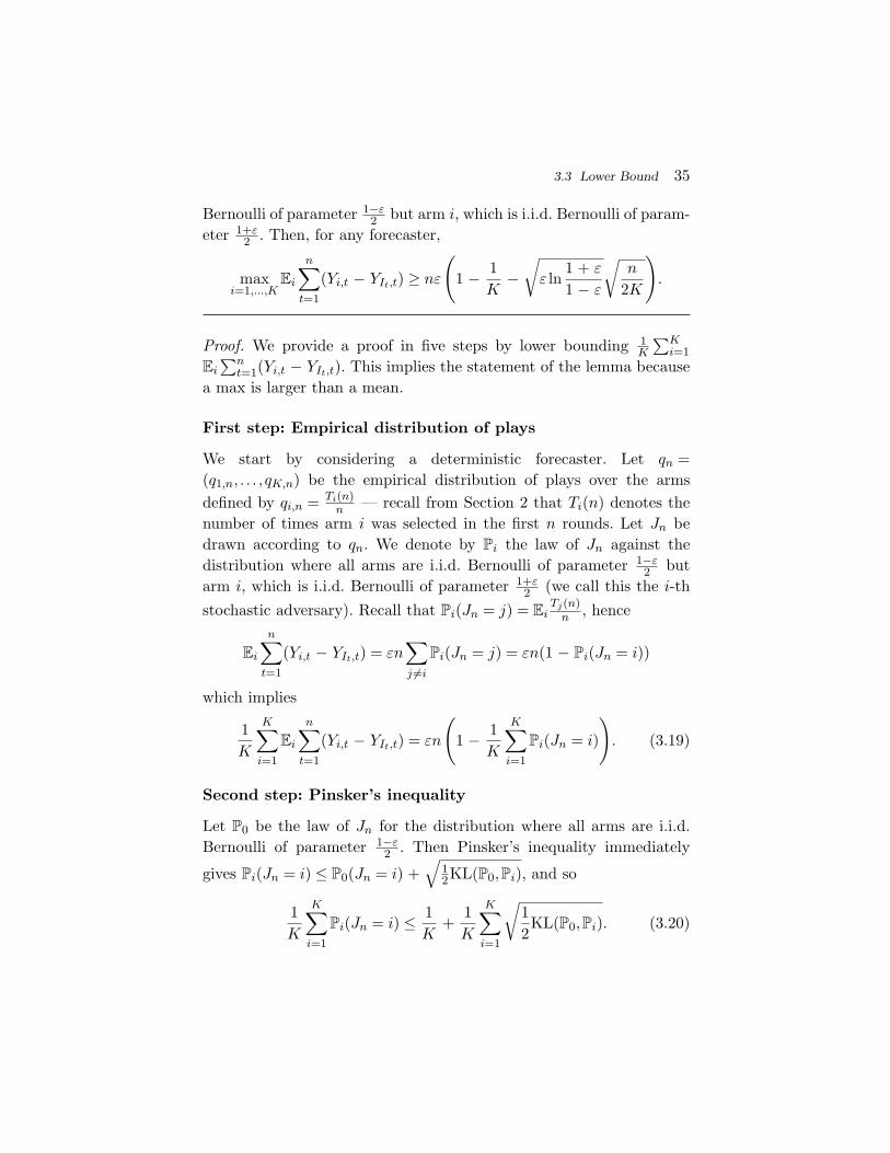
3.3 Lower Bound 35
Bernoulli of parameter 1−ε2 but arm i, which is i.i.d. Bernoulli of param-
eter 1+ε2 . Then, for any forecaster,
maxi=1,...,K
Ei
n∑t=1
(Yi,t − YIt,t) ≥ nε(
1 − 1K−√ε ln
1 + ε
1 − ε√
n
2K
).
Proof. We provide a proof in five steps by lower bounding 1K
∑Ki=1
Ei∑n
t=1(Yi,t − YIt,t). This implies the statement of the lemma becausea max is larger than a mean.
First step: Empirical distribution of plays
We start by considering a deterministic forecaster. Let qn =(q1,n, . . . , qK,n) be the empirical distribution of plays over the armsdefined by qi,n = Ti(n)
n — recall from Section 2 that Ti(n) denotes thenumber of times arm i was selected in the first n rounds. Let Jn bedrawn according to qn. We denote by Pi the law of Jn against thedistribution where all arms are i.i.d. Bernoulli of parameter 1−ε
2 butarm i, which is i.i.d. Bernoulli of parameter 1+ε
2 (we call this the i-thstochastic adversary). Recall that Pi(Jn = j) = Ei
Tj(n)n , hence
Ei
n∑t=1
(Yi,t − YIt,t) = εn∑j =i
Pi(Jn = j) = εn(1 − Pi(Jn = i))
which implies
1K
K∑i=1
Ei
n∑t=1
(Yi,t − YIt,t) = εn
(1 − 1
K
K∑i=1
Pi(Jn = i)
). (3.19)
Second step: Pinsker’s inequality
Let P0 be the law of Jn for the distribution where all arms are i.i.d.Bernoulli of parameter 1−ε
2 . Then Pinsker’s inequality immediately
gives Pi(Jn = i) ≤ P0(Jn = i) +√
12KL(P0,Pi), and so
1K
K∑i=1
Pi(Jn = i) ≤ 1K
+1K
K∑i=1
√12KL(P0,Pi). (3.20)

36 Adversarial Bandits: Fundamental Results
Third step: Computation of KL(P0,Pi)
Since the forecaster is deterministic, the sequence of rewards Y n =(Y1, . . . ,Yn) ∈ 0,1n received by the forecaster uniquely determines theempirical distribution of plays qn. In particular, the law of Jn condi-tionally to Y n is the same for any i-th stochastic adversary. For eachi = 0, . . . ,K, let P
ni be the law of Y n against the i-th adversary. Then
one can easily show that KL(P0,Pi) ≤ KL(Pn0 ,Pni ). Now we use the
chain rule for Kullback–Leibler divergence — see for example [61, Sec-tion A.2] — iteratively to introduce the laws P
ti of Y t = (Y1, . . . ,Yt).
More precisely, we have
KL(Pn0 ,Pni )
= KL(P10,P
1i ) +
n∑t=2
∑yt−1
Pt−10 (yt−1)KL(Pt0(· | yt−1),Pti(· | yt−1))
= KL(P10,P
1i ) +
n∑t=2
∑yt−1 :It=i
Pt−10 (yt−1)KL
(1 − ε
2,1 + ε
2
)
+∑
yt−1 :It =iPt−10 (yt−1)KL
(1 + ε
2,1 + ε
2
)= KL
(1 − ε
2,1 + ε
2
)E0Ti(n). (3.21)
Fourth step: Conclusion for deterministic forecasters
By using that the square root is concave and combining KL(P0,Pi) ≤KL(Pn0 ,P
ni ) with Equation (3.21), we deduce that
1K
K∑i=1
√KL(P0,Pi) ≤
√√√√ 1K
K∑i=1
KL(P0,Pi)
≤√√√√ 1K
K∑i=1
KL(
1 − ε2
,1 + ε
2
)E0Ti(n)
=
√n
KKL(
1 − ε2
,1 + ε
2
). (3.22)

3.4 Refinements and Bibliographic Remarks 37
We conclude the proof for deterministic forecasters by applyingEquations (3.20) and (3.22) to Equation (3.19), and observing thatKL(1−ε
2 , 1+ε2 ) = ε ln 1+ε
1−ε .
Fifth step: Randomized forecasters via Fubini’s Theorem
Extending previous results to randomized forecasters is easy. Denoteby Er the expectation with respect to the forecaster’s internal random-ization. Then Fubini’s Theorem implies
1K
K∑i=1
Ei
n∑t=1
Er(Yi,t − YIt,t) = Er1K
K∑i=1
Ei
n∑t=1
(Yi,t − YIt,t).
Now the proof is concluded by applying the lower bound on1K
∑Ki=1 Ei
∑nt=1(Yi,t − YIt,t), which we proved in previous steps, to each
realization of the forecaster’s random bits.
3.4 Refinements and Bibliographic Remarks
The adversarial framework studied in this section was originally inves-tigated in a full information setting, where at the end of each roundthe forecaster observes the complete loss vector (1,t, . . . , K,t). We referthe reader to [61] for the history of this problem. The Exp3 and Exp3.Pstrategies were introduced1 and analyzed by Auer et al. [24], where thelower bound of Theorem 3.5 is also proven. The proofs presented inthis section are taken from Ref. [43]. We now give an overview of someof the many improvements and refinements that have been proposedsince these initial analyses.
3.4.1 Log-Free Upper Bounds
One can see that there is a logarithmic gap between the pseudo-regretof Exp3, presented in Theorem 3.1, and the minimax lower bound ofTheorem 3.5. This gap was closed by Audibert and Bubeck [17], whoconstructed a new class of strategies and showed that some of them
1 In its original formulation the Exp3 strategy was defined as a mixture of exponentialweights with the uniform distribution on the set of arms. It was noted in Stoltz [156] thatthis mixing is not necessary, see footnote 2 on page 26 in Bubeck [43] for more details onthis.

38 Adversarial Bandits: Fundamental Results
have a pseudo-regret of order√nK. This new class of strategies, called
INF (Implicitly Normalized Forecaster), is based on the following idea.First, note that one can generalize the exponential weighting schemeof Exp3 as follows: given a potential function ψ, assign the probability
pi,t+1 =ψ(Li,t)∑Kj=1ψ(Lj,t)
.
This type of strategy is called a weighted average forecaster, see [61,Section 2]. In INF the normalization is done implicitly, by a translationof the losses. More precisely, INF with potential ψ assigns the probabil-ity pi,t+1 = ψ(Ct − Li,t), where Ct is the constant such that pt+1 sumto 1. The key to obtain a minimax optimal pseudo-regret is to takeψ of the form ψ(x) = (−ηx)−q with q > 1, while Exp3 corresponds toψ(x) = exp(ηx). Audibert et al. [19] realized that the INF strategy canbe formulated as a Mirror Descent algorithm. This point of view sig-nificantly simplifies the proofs. We refer the reader to Section 5 (andin particular Theorem 5.10) for more details.
While it is possible to get log-free pseudo-regret bounds, the sit-uation becomes significantly more complicated when one considershigh probability regret and expected regret. Audibert and Bubeck [18]proved that one can get a log-free expected regret if the adversary isoblivious, i.e., the sequence of loss vectors is independent of the fore-caster’s actions. Moreover, it is also possible to get a log-free high prob-ability regret if the adversary is fully oblivious (i.e., the loss vectors areindependently drawn, but not identically distributed — this includesthe oblivious adversary). It is conjectured [18] that it is not possible toobtain a log-free expected regret bound against a general nonobliviousadversary.
3.4.2 Adaptive Bounds
One of the strengths of the bounds proposed in this section is also oneof its weaknesses: the bounds hold against any adversary. It is clearthat in some cases it is possible to obtain a much smaller regret thanthe worst case regret. For example, when the sequence of losses is ani.i.d. sequence, we proved in Section 2 that it is possible to obtain a
3.4 Refinements and Bibliographic Remarks 39
logarithmic pseudo-regret (provided that the gap ∆ is considered as aconstant). Thus, it is natural to ask if it is possible to have strategieswith minimax optimal regret, but also with much smaller regret whenthe loss sequence is not worst case.
The first bound in this direction was proved by Auer et al.[24], whoshowed that, for the gain version of the problem and against an obliv-ious adversary, Exp3 has a pseudo-regret of order
√KG∗
n (omittinglog factors), where G∗
n ≤ n is the maximal cumulative reward of theoptimal arm after n rounds. This result was improved by Audibert andBubeck [18], who showed that using the gain estimate
gi,t = − It=i
βln(
1 − βgi,tpi,t
)one can bound the regret with high probability by essentially the samequantity as before, and against any adversary.
Another direction was explored by Hazan and Kale [96] buildingon previous works in the full information setting — [64]. In this work
the authors proved that one can attain a regret of order√∑K
i=1Vi,nexcluding log factors, where
Vi,n =n∑t=1
(i,t − 1
n
n∑s=1
i,s
)2
is the total variation of the loss for arm i. In fact their result is moregeneral, as it applies to the linear bandit framework — see Section 5.The main new ingredient in their analysis is a “reservoir sampling”procedure. We refer the reader to [96] for details. See also the works ofSlivkins and Upfal [153] and Slivkins [152] for related results on slowlychanging bandits.
In Section 3.4.4 below we describe another type of adaptive bound,where one combines minimax optimal regret for the adversarial modelwith logarithmic pseudo-regret for the stochastic model.
3.4.3 Competing with the Best Switching Strategy
While competing against the policy consistently playing the best fixedarm is a natural way of defining regret, in some applications it might be

40 Adversarial Bandits: Fundamental Results
interesting to consider regret with respect to a bigger class of policies.Though this problem is the focus of Section 4, there is a class of naturalpolicies that can be directly dealt with by the methods of this section.Namely, consider the problem of competing against any policy con-strained to make at most S ≤ n switches (a switch is when the armplayed at time t is different from the arm played at time t + 1). Thisproblem was studied by Auer [22], where it was first shown that asimple variant of Exp3 attains a low switching regret against oblivi-ous adversaries. Later, Audibert and Bubeck [18] proved that Exp3.Pattains an expected regret (and a high probability regret) of order√nKS ln(nK/S) for this problem.
3.4.4 Stochastic versus Adversarial Bandits
From a practical viewpoint, Exp3 should be a safe choice whenwe have reasons to believe that the sequence of rewards is notwell matched by any i.i.d. process. Indeed, it is easy to prove thatUCB can have linear regret, i.e., Rn = Ω(n), on certain determin-istic sequences. In [53] a new strategy was described, called SAO(Stochastic and Adversarial Optimal), which enjoys (up to logarith-mic factors) both the guarantee of Exp3 for the adversarial modeland the guarantee of UCB for the stochastic model. More preciselySAO satisfies Rn = O(K∆ log2(n) log(K)) in the stochastic model andRn = O(
√nK log3/2(n) log(K)) in the adversarial model. Note that
while this result is a step toward more flexible strategies, the very notionof regret Rn can become vacuous with nonstationarities in the rewardsequence, since the total reward of the best fixed action might be verysmall. In that case the notion of switching regret — see Section 3.4.3 —is more relevant, and it would be interesting to derive a strategy withlogarithmic regret in the stochastic model, and a switching regret oforder
√nKS in the adversarial model.
3.4.5 Alternative Feedback Structures
As mentioned at the beginning of this section, the adversarial multi-armed bandit is a variation of the full information setting, with a weakerfeedback signal (only the incurred loss versus the full vector of losses is

3.4 Refinements and Bibliographic Remarks 41
observed). Many other feedback structures can be considered, and weconclude the section by describing a few of them.
In the label efficient setting, originally proposed by Helmbold andPanizza [99], at the end of each round the forecaster has to decidewhether to ask for the losses of the current round, knowing that thiscan be done for at most m ≤ n times. In this setting, Cesa-Bianchi
et al. [63] proved that the minimax pseudo-regret is of order n√
lnKm .
A bandit label efficient version was proposed by Allenberg et al. [11].Audibert and Bubeck [18] proved that the minimax pseudo-regret for
the bandit label efficient version is of order n√
Km . These results do not
require any fundamentally new algorithmic idea, besides the fact theforecaster has to randomize to select the rounds in which the losses arerevealed. Roughly speaking, a simple coin toss with parameter ε = m/n
is sufficient to obtain an optimal regret.Mannor and Shamir [133] study a model that interpolates between
the full information and the bandit setting. The basic idea is that thereis an undirected graph G with K vertices (one vertex for each arm)that encodes the feedback structure. When one pulls arm i the lossesof all neighboring arms j ∈ N(i) in the graph are observed. Thus, agraph with no edges is equivalent to the bandit problem, while thecomplete graph is equivalent to the full information setting. Given thefeedback structure G, it is natural to consider the following unbiasedloss estimate
i,t =i,t i∈N(It)∑j∈N(i) pj,t
.
Using Exp3 with this loss estimate, the authors show that the mini-max pseudo-regret (up to logarithmic factors) is of order of
√α(G)n,
where α(G) is the independence number of graph G. Note that thisinterpolated setting naturally arises in applications like ad placementon websites. Indeed, if a user clicks on an advertisement, it is plausibleto assume that the same user would have clicked on similar advertise-ments, had they been displayed.
The above problems are all specific examples of the more generalpartial monitoring setting. In this model, at the end of each round the

42 Adversarial Bandits: Fundamental Results
player does not observe the incurred loss It,t but rather a stochastic“signal” SIt,t. A prototypical example of this scenario is the following:a website is repeatedly selling the same item to a sequence of cus-tomers. The selling price is dynamically adjusted, and each customerbuys the item only if the current price is smaller or equal than his ownhidden value for the item. The pricing algorithm (i.e., the player in ourterminology) does not see each user’s value, but only whether the userbought the item or not.
The relationship between the signals and the incurred losses definesthe instance of a partial monitoring problem. We refer the interestedreader to [61] for more details, including an historical account. Recentprogress on this problem has been made by Bartok et al. [34, 35] andFoster and Rakhlin [80].

4Contextual Bandits
A natural extension of the multi-armed problem is obtained by associ-ating side information with each arm. Based on this side information, orcontext, a notion of “contextual regret” is introduced where optimalityis defined with respect to the best policy (i.e., mapping from contextsto arms) rather than the best arm. The space of policies, within whichthe optimum is sought, is typically chosen in order to have some desiredstructure. A different viewpoint is obtained when the contexts are pri-vately accessed by the policies (which are then appropriately called“experts”). In this case the contextual information is hidden from theforecaster, and arms must be chosen based only on the past estimatedperformance of the experts.
Contextual bandits naturally arise in many applications. For exam-ple, in personalized news article recommendation the task is to select,from a pool of candidates, a news article to display whenever a newuser visits a website. The articles correspond to arms, and a rewardis obtained whenever the user clicks on the selected article. Side infor-mation, in the form of features, can be extracted from both user andarticles. For the user this may include historical activities, demographicinformation, and geolocation; for the articles, we may have content
43

44 Contextual Bandits
information and categories. See [128] for more details on this applica-tion of contextual bandits.
In general, the presence of contexts creates a wide spectrum of possi-ble variations obtained by combining assumptions on the rewards withassumptions on the nature of contexts and policies. In this section wedescribe just a few of the results available in the literature and use thebibliographic remarks to mention all those that we are aware of.
4.1 Bandits with Side Information
The most basic example of contextual bandits is obtained when gamerounds t = 1,2, . . . are marked by contexts s1,s2, . . . from a given contextset S. The forecaster must learn the best mapping g : S → 1, . . . ,K ofcontexts to arms. We analyze this simple side information setting in thecase of adversarial rewards, and we further assume that the sequence ofcontexts st is arbitrary but fixed. The approach we take is the simplest:run a separate instance of Exp3 on each distinct context.
We introduce the following notion of pseudo-regret
RSn = max
g :S→1,...,KE
[n∑t=1
It,t −n∑t=1
g(st),t
].
Here st ∈ S denotes the context marking the t-th game round. A boundon this pseudoregret is almost immediately obtained using the adver-sarial bandit results from Section 3.
Theorem 4.1. There exists a randomized forecaster for bandits withside information (the S-Exp3 forecaster, defined in the proof) thatsatisfies
RSn ≤√
2n|S|K lnK
for any set S of contexts.
Proof. Let S = |S|. The S-Exp3 forecaster runs an instance of Exp3on each context s ∈ S. Let ns the number of times when st = s withinthe first n time steps. Using the bound (Equation (3.2)) established in

4.2 The Expert Case 45
Theorem 3.1 we get
maxg :S→1,...,K
E
[n∑t=1
(It,t − g(st),t)
]=∑s∈S
maxk=1,...,K
E
[ ∑t :st=s
(It,t − k,t)]
≤∑s∈S
√2nsK lnK
≤√
2nSK lnK
where in the last step we used Jensen’s inequality and the identity∑sns = n.
In Section 4.2.1, we extend this construction by considering severalcontext sets simultaneously.
A lower bound Ω(√nSK) is an immediate consequence of the adver-
sarial bandit lower bound (Theorem 3.5) under the assumption that aconstant fraction of the contexts in S marks at least constant fractionof the n game rounds.
4.2 The Expert Case
We now consider the contextual variant of the basic adversarial banditmodel of Section 3. In this variant there is a finite set of N random-ized policies. Following the setting of prediction with expert advice, noassumptions are made on the way policies compute their randomizedpredictions, and the forecaster experiences the contexts only throughthe advice provided by the policies. For this reason, in what follows weuse the word expert to denote a policy. Calling this a model of con-textual bandits may sound a little strange, as the structure of contextsdoes not seem to play a role here. However, we have decided to includethis setting in this section because bandit with experts have been usedin practical contextual bandit problems — see, e.g., the news recom-mendation experiment in Ref. [40].
Formally, at each step t = 1,2, . . . the forecaster obtains the expertadvice (ξ1t , . . . , ξ
Nt ), where each ξjt is a probability distribution over
arms representing the randomized play of expert j at time t. Ift = (1,t, . . . , K,t) ∈ [0,1]K is the vector of losses incurred by the K
46 Contextual Bandits
arms at time t, then Ei∼ξj
ti,t denotes the expected loss of expert j at
time t. We allow the expert advice to depend on the realization of theforecaster’s past random plays. This fact is explicitly used in the proofof Theorem 4.5.
Similarly to the pseudo-regret (Equation (3.1)) for adversarial ban-dits, we now introduce the pseudo-regret Rctx
n for the adversarial con-textual bandit problem,
Rctxn = max
i=1,...,NE
[n∑t=1
It,t −n∑t=1
Ek∼ξitk,t
].
In order to bound the contextual pseudo-regret Rctxn , one could
naively use Exp3 strategy of Section 3 on the set of experts. Thiswould give a bound of order
√nN logN . In Figure 4.1 we introduce
the contextual forecaster Exp4 for which we show a bound of order√nK lnN . Thus, in this framework we can be competitive even with
an exponentially large (with respect to n) number of experts.Exp4 is a simple adaptation of Exp3 to the contextual setting. Exp4
runs Exp3 over the N experts using estimates of the experts’ lossesEi∼ξj
ti,t. In order to draw arms, Exp4 mixes the expert advice with the
probability distribution over experts maintained by Exp3. The resultingbound on the pseudo-regret is of order
√nK lnN , where the term
√lnN
comes from running Exp3 over the N experts, while√K is a bound on
the second moment of the estimated expert losses under the distributionqt computed by Exp3. Equation (4.6) shows that Ej∼qt y2
j,t ≤ Ei∼pt 2i,t.
That is, this second moment is at most that of the estimated arm lossesunder the distribution pt computed by Exp4, which in turn is boundedby√K using techniques from Section 3.
Theorem 4.2(Pseudo-regret of Exp4). Exp4 without mixing and
with ηt = η =√
2lnNnK satisfies
Rctxn ≤
√2nN lnK. (4.1)
On the other hand, with ηt =√
lnNtK it satisfies
Rctxn ≤ 2
√nN lnK. (4.2)
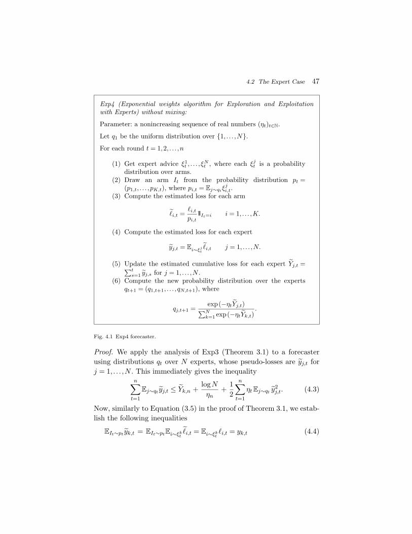
4.2 The Expert Case 47
Exp4 (Exponential weights algorithm for Exploration and Exploitationwith Experts) without mixing:
Parameter: a nonincreasing sequence of real numbers (ηt)t∈N.
Let q1 be the uniform distribution over 1, . . . ,N.For each round t = 1,2, . . . ,n
(1) Get expert advice ξ1t , . . . , ξNt , where each ξj
t is a probabilitydistribution over arms.
(2) Draw an arm It from the probability distribution pt =(p1,t, . . . ,pK,t), where pi,t = Ej∼qt
ξji,t.
(3) Compute the estimated loss for each arm
i,t =i,tpi,t
It=i i = 1, . . . ,K.
(4) Compute the estimated loss for each expert
yj,t = Ei∼ξjti,t j = 1, . . . ,N.
(5) Update the estimated cumulative loss for each expert Yj,t =∑ts=1 yj,s for j = 1, . . . ,N .
(6) Compute the new probability distribution over the expertsqt+1 = (q1,t+1, . . . , qN,t+1), where
qj,t+1 =exp(−ηtYj,t)∑N
k=1 exp(−ηtYk,t).
Fig. 4.1 Exp4 forecaster.
Proof. We apply the analysis of Exp3 (Theorem 3.1) to a forecasterusing distributions qt over N experts, whose pseudo-losses are yj,t forj = 1, . . . ,N . This immediately gives the inequality
n∑t=1
Ej∼qt yj,t ≤ Yk,n +logNηn
+12
n∑t=1
ηtEj∼qt y2j,t. (4.3)
Now, similarly to Equation (3.5) in the proof of Theorem 3.1, we estab-lish the following inequalities
EIt∼pt yk,t = EIt∼ptEi∼ξkti,t = Ei∼ξk
ti,t = yk,t (4.4)
48 Contextual Bandits
Ej∼qt yj,t = Ej∼qtEi∼ξjti,t = Ei∼pt i,t = It,t (4.5)
Ej∼qt y2j,t = Ej∼qt(Ei∼ξj
ti,t)2 ≤ Ej∼qtEi∼ξj
t2i,t = Ei∼pt
2i,t =
2It,tpIt,t
(4.6)
where we used Jensen’s inequality to prove Equation (4.6). By applyingEquations (4.5) and (4.6) to Equation (4.3) we get
n∑t=1
It,t =n∑t=1
Ej∼qt yj,t ≤ Yk,n +logNηn
+12
n∑t=1
ηt2It,tpIt,t
.
Now note that, if we take expectation over the draw of I1, . . . , In, usingEquation (4.4) we obtain
E Yk,n = E
[n∑t=1
E[yj,n|I1, . . . , It−1]
]= E
[n∑t=1
Ei∼ξkti,t
]= EYk,n.
Hence,
Rctxn = max
k=1,...,NE
[n∑t=1
It,t − Yk,n]≤ logN
ηn+K
2
n∑t=1
ηt.
Choosing ηt as in the statement of the theorem, and using the inequality∑nt=1 t
−1/2 ≤ 2√n, concludes the proof.
Besides pseudo-regret, the contextual regret
Rctxn = max
k=1,...,N
(n∑t=1
It,t −n∑t=1
Ei∼ξJti,t
)
can be also bounded, at least with high probability. Indeed, similarly tothe variant Exp3.P of Exp3 (see Section 3.2), an analogous modificationof Exp4, called Exp4.P, satisfies
Rctxn ≤ c
√nK ln(Nδ−1)
for some constant c > 0 and with probability at least 1 − δ, whereδ ∈ (0,1) is a parameter of the algorithm.
4.2 The Expert Case 49
4.2.1 Competing Against the Best Context Set
We revisit the basic contextual scenario introduced in Section 4.1,where the goal is to compete against the best mapping from contextsto arms. Consider now a class Sθ : θ ∈ Θ of context sets. In this newgame, each time step t = 1,2, . . . is marked by the vector (sθ,t)θ∈Θ ofcontexts, one for each set in Θ. Introduce the pseudoregret
RΘn = max
θ∈Θmax
g :Sθ→1,...,KE
[n∑t=1
It,t −n∑t=1
g(sθ,t),t
].
When |Θ| = 1 we recover the contextual pseudoregret RSn . In general,
when Θ contains more than one set, the forecaster must learn both thebest set Sθ and the best function g : Sθ → 1, . . . ,K from that set tothe set of arms.
We find this variant of contextual bandits interesting because itssolution involves a nontrivial combination of two of the main algo-rithms examined in this section: Exp4 and S-Exp3. In particular, weconsider a scenario in which Exp4 uses instances of S-Exp3 as experts.The interesting aspect is that these experts are learning themselves,and thus the analysis of the combined algorithm requires taking intoaccount the learning process at both levels.
Note that in order to solve this problem we could simply lump allcontexts in a big set and use the proof of Theorem 4.1. However, thiswould give a regret bound that depends exponentially in |Θ|. On theother hand, by using Exp4 directly on the set of all policies g (which is ofcardinality exponential in |Θ| × |S|), we could improve this to a boundthat scales with
√|Θ|. The idea we explore here is to use Exp4 overthe class Θ of “experts” and combine this with the S-Exp3 algorithmof Theorem 4.1. This gets us down to a logarithmic dependency on |Θ|,albeit at the price of a worse dependency on n.
Intuitively, Exp4 provides competitiveness against the best contextset Sθ, while the instances of the S-Exp3 algorithm, acting as expertsfor Exp4, ensure that we are competitive against the best function g :Sθ → 1, . . . ,K for each θ ∈ Θ. However, by doing so we immediatelyrun into a problem: the pt used by Exp4 is not the same as the pt’sused by each expert. In order to address this issue, we now show that

50 Contextual Bandits
the analysis of Exp3 holds even when the sequence of plays I1, I2, . . . isdrawn from a sequence of distributions q1, q2, . . . possibly different fromthe one chosen by the forecaster. The only requirement we need is thateach probability in qt be bounded away from zero.
Theorem 4.3. Consider a K-armed bandit game in which at each stept = 1,2, . . . the played arm It is drawn from an arbitrary distributionqt over arms. Each qt may depend in an arbitrary way on the pairs(I1, I1,1), . . . ,(It−1, It−1,t−1). Moreover, qt,i ≥ ε > 0 for all i = 1, . . . ,Kand t ≥ 1.
If Exp3 without mixing is run with i,t = i,tqi,t It=i and ηt = η =√
2lnKnK then
maxk=1,...,K
EIn∼qn
[n∑t=1
Ei∼pti,t −n∑t=1
k,t
]≤√
2nε
lnK (4.7)
where In ∼ qn means that each It is drawn from qt for t = 1, . . . ,n, andpt is the distribution used by Exp3 at time t.
Proof. The proof is an easy adaptation of Exp3 analysis (Theorem 3.1in Section 3) and we just highlight the differences. The key step is theanalysis of the log moment of i,t:
Ei∼pt i,t =1η
logEi∼pt exp(−η(i,t − Ek∼pt k,t))
−1η
logEi∼pt exp(−ηi,t).
The first term is bounded in a manner slightly different from the proofof Theorem 3.1,
logEi∼pt exp(−η(i,t − Ek∼pt k,t)) ≤η2
2Ei∼pt
2i,t ≤
η2
2pIt,tq2It,t
.
The analysis of the second term is unchanged: Let Li,0 = 0, Φ0(η) = 0and Φt(η) = 1
η log 1K
∑Ki=1 exp(−ηLi,t). Then by definition of pt we have:
−1η
logEi∼pt exp(−ηi,t) = Φt−1(η) − Φt(η).

4.2 The Expert Case 51
Proceeding again as in the proof of Theorem 3.1 we obtain
EIn∼qn
[n∑t=1
Ei∼pt i,t
]≤ EIn∼qn
[n∑t=1
k,t +η
2pIt,tq2It,t
]+
lnKη
.
Now observe that
EIt∼qt k,t = k,t and EIt∼qtpIt,tq2It,t
=K∑i=1
pi,tqi,t≤ 1ε.
Therefore,
EIn∼qn
[n∑t=1
(Ei∼pti,t − k,t)]
= EIn∼qn
[n∑t=1
(Ei∼pt i,t − k,t)]
≤ ηn
2ε+
lnKη
.
Choosing η as in the statement of the theorem concludes the proof.
It is left to the reader to verify that the analysis of S-Exp in Theo-rem 4.1 can be combined with the above analysis to give the bound
maxg :S→1,...,K
EIn∼qn
[n∑t=1
Ei∼pti,t −n∑t=1
g(st),t
]≤√
2nε|S| lnK.
(4.8)
Next, we state a bound on the contextual pseudoregret of a variantof Exp4 whose probabilities pi,t satisfy the property pi,t ≥ γ
K for alli = 1, . . . ,K and t ≥ 1, where γ > 0 is a parameter. This is obtained byreplacing in Exp4 the assignment pi,t = Ej∼qtξ
ji,t (line 2 in Figure 4.1)
with the assignment
pi,t = (1 − γ)Ej∼qtξji,t +γ
K
where γ > 0 is the mixing coefficient. This mixing clearly achieves thedesired property for each pi,t.
Theorem 4.4 (Pseudo-regret of Exp4 with mixing). Exp4 withmixing coefficient γ and with ηt = η = γ/K satisfies
Rctxn ≤
γn
2+K lnNγ
. (4.9)
52 Contextual Bandits
Proof. The proof goes along the same lines of Exp4 original proof [24,Theorem 7.1] with the following modifications: since the weights arenegative exponentials, we can use the bound exp(−x) ≤ 1 − x + x2
2for all x ≥ 0 rather than exp(x) ≤ 1 + x + (e − 2)x2 for all 0 ≤ x ≤ 1;the term (1 − γ)∑t k,t is upper bounded directly by
∑t k,t; the term
γK
∑t
∑i i,t is upper bounded by γn without requiring the assumption
that the expert set contains the “uniform expert”. Finally, the factthat experts’ distributions ξjt depend on the realization of past fore-caster’s random arms is dealt with in the same way as in the proof ofTheorem 4.2.
Theorem 4.5. There exists a randomized forecaster achieving
RΘn = O
(n2/3(
maxθ∈Θ|Sθ|K lnK
)1/3√ln |Θ|
)for any class Sθ : θ ∈ Θ of context sets.
Proof. We run the Exp4 forecaster with mixing coefficient γ usinginstances of the S-Exp3 algorithm (defined in the proof of Theorem 4.1)as experts. Each S-Exp3 instance is run on a different context set Sθfor θ ∈ Θ. Let ξθt be the distribution used at time t by the S-Exp3instance running on context set Sθ and let pn be the joint distributionof In = (I1, . . . , In) used by Exp4. Since pi,t ≥ γ
K for all i = 1, . . . ,K andt ≥ 1, we can use Equation (4.8) with ε = γ/K. Thus, Theorem 4.4implies
EIn∼pn
[n∑t=1
It,t
]≤ min
θ∈ΘEIn∼pn
[n∑t=1
Ek∼ξθtk,t
]+γn
2+K ln |Θ|
γ
≤ minθ∈Θ
ming :Sθ→1,...,K
E
[n∑t=1
g(st),t
]
+√
2nε
maxθ∈Θ|Sθ| lnK +
γn
2+K ln |Θ|
γ.
Substituting ε = γ/K in the above expression and choosing γ of theorder of n−1/3(maxθ∈Θ |Sθ|K lnK)1/3
√ln |Θ| gives the desired result.
4.3 Stochastic Contextual Bandits 53
Note that in Theorem 4.5 the rate is n2/3, in contrast to the moreusual n1/2 bandit rate. This worsening is inherent in the Exp4-over-Exp3 construction. It is not known whether the rate could be improvedwhile keeping the same logarithmic dependence on |Θ| guaranteed bythis construction.
4.3 Stochastic Contextual Bandits
We now move on to consider the case in which policies have a knownstructure. More specifically, each policy is a function f mapping thecontext space to the arm space 1, . . . ,K and the set F of policies isgiven as an input parameter to the forecaster.
Under this assumption on the policies, the problem can be viewedas a bandit variant of supervised learning. For this reason, here and inthe next section we follow the standard notation of supervised learningand use x rather than s to denote contexts.
In supervised learning, we observe data of the form (xt, t). In thecontextual bandit setting, the observed data are (xt, It,t) where It is thearm chosen by the forecaster at time t given context xt ∈ X . This con-nection to supervised learning has steered the focus of research towardstochastic data generation models, which are widespread in the analysisof supervised learning. In the stochastic variant of contextual bandits,contexts xt and arm losses t = (1,t, . . . , K,t) are realizations of i.i.d.draws from a fixed and unknown distribution D over X × [0,1]K . Intight analogy with statistical learning theory, a policy f is evaluated interms of its statistical risk D(f) = E(x,)∼Df(x). Let
f∗ = arginff∈F
D(f)
the risk-minimizing policy in the class. The regret with respect to theclass F of a forecaster choosing arms I1, I2, . . . is then defined by
n∑t=1
It,t − nD(f∗).
This can be viewed as the stochastic counterpart of the adversarialcontextual regret Rctx
n introduced in Section 4.2. The main question is

54 Contextual Bandits
now to characterize the “price of bandit information” using the samplecomplexity of supervised learning as yardstick.
In the rest of this section we focus on the case of K = 2 arms andparameterize classes F of policies f : X → 1,2 by their VC-dimensiond — see [41] for a modern introduction to VC theory. For this setting,we consider the following forecaster.
VE (VC dimension by Exponentiation):
Parameters: number n of rounds, n′ satisfying 1 ≤ n′ ≤ n.
(1) For the first n′ rounds, choose arms uniformly at random.(2) Build F ′ ⊆ F such that for any f ∈ F there is exactly
one f ′ ∈ F ′ satisfying f(xt) = f ′(xt) for all t = 1, . . . ,n′.(3) For t = n′ + 1, . . . ,n play by simulating Exp4.P using the
policies of F ′ as experts.
We now show that the per round regret of VE is of order√d/n, exclud-
ing logarithmic factors. This rate is equal to the optimal rate for super-vised learning of VC-classes, showing that — in this case — the priceof bandit information is essentially zero.
Theorem 4.6. For any class F of binary policies f : X → 0,1 ofVC-dimension d and for all n > d, the forecaster VE run with n′ =√n(2d ln en
d + ln 3δ
)satisfies
n∑t=1
It,t − n inff∈F
D(f) ≤ c√n
(d ln
en
d+ ln
3δ
)(4.10)
for some constant c > 0 and with probability at least 1 − δ with respectto both the random data generation and VE’s internal randomization.
Proof. Given a sample realization (x1, 1), . . . ,(xn, n), let f ′ be theunique element of F ′ such that f ′(xt) = f∗(xt) for all t = 1, . . . ,n′,where f∗ is the risk-minimizing function in F . Given a sample, without

4.3 Stochastic Contextual Bandits 55
loss of generality we may assume that F contains functions restrictedon the finite domain x1, . . . ,xn. Recall Sauer–Shelah lemma — see,e.g., [41] — stating that any class F of binary functions defined ona finite domain of size n satisfies |F| ≤ ( end )d, where d is the VC-dimension of F . Then, with probability at least 1 − δ
3 with respectto VE’s internal randomization,n∑t=1
It,t ≤ n′ +n∑
t=n′+1
f ′(xt),t + c
√2(n − n′) ln
3|F ′|δ
≤ n′ +n∑
t=n′+1
(f∗(xt),t + f ′(xt),t − f∗(xt),t)
+c
√2(n − n′) ln
3|F ′|δ
≤ n′ +n∑
t=n′+1
(f∗(xt),t + f ′(xt) =f∗(xt)) + c
√2(n − n′) ln
3|F ′|δ
≤ n′ +n∑
t=n′+1
(f∗(xt),t + f ′(xt) =f∗(xt))
+c
√2n(d ln
en
d+ ln
3δ
)where we used i,t ∈ [0,1] in the penultimate step and the Sauer–Shelahlemma in the last step. Now, the term
∑t f∗(xt),t is controlled in prob-
ability w.r.t. the random draw of the sample via Chernoff bounds,
P
(n∑
t=n′+1
f∗(xt),t > (n − n′)D(f∗) +
√n − n′
2ln
3δ
)≤ δ.
Hence,n∑t=1
It,t ≤ n′ + nD(f∗)
+n∑
t=n′+1f ′(xt) =f∗(xt) + c
√2n(d ln
en
d+ ln
3δ
)
56 Contextual Bandits
with probability at least 2δ3 with respect to both the random sample
draw and VE’s internal randomization.The term
∑t f ′(xt) =f∗(xt) quantifies the fact that the unique func-
tion f ′ ∈ F ′ that agrees with f∗ on the first n′ data points is generallydifferent from f∗ on the remaining n − n′ points. Since each data point(xt, t) is drawn i.i.d., the distribution of a sequence of n pairs remainsthe same if we randomly permute their positions after drawing them.Hence we can bound
∑t f ′(xt) =f∗(xt) in probability w.r.t. a random
permutation σ of 1, . . . ,n. Let ‖f − g‖ =∑n
t=1 f ′(xt) =f∗(xt). Then
Pσ
(n∑
t=n′+1f ′(xσ(t)) =f∗(xσ(t)) > k
)≤ Pσ
(∃f,g ∈ F , ‖f − g‖ > k : f(xσ(t)) = g(xσ(t)), t = 1, . . . ,n′)≤ |F|2
(1 − k
n
)n′
≤(end
)2dexp(−kn
′
n
)≤ δ
3for
k ≥ n
n′
(2d ln
en
d+ ln
3δ
).
Now, since we just proved thatn∑
t=n′+1f ′(xσ(t)) =f∗(xσ(t)) ≤
n
n′
(2d ln
en
d+ ln
3δ
)holds with probability at least δ
3 for any sample realization, it holdswith the same probability for a random sample. Hence, by choosing n′
as in the statement of the theorem and overapproximating, we get thedesired result.
4.4 The Multiclass Case
A different viewpoint on contextual bandits is provided by the so-calledbandit multiclass problem. This is a bandit variant of the online

4.4 The Multiclass Case 57
protocol for multiclass classification, where the goal is to sequentiallylearn a mapping from the context space R
d to the label space 1, . . . ,K,with K ≥ 2. In this protocol the learner keeps a classifier parameterizedby aK × dmatrixW . At each time step t = 1,2, . . . the side informationxt ∈ R
d is observed (following standard notations in online classifica-tion, here we use x instead of s to denote contexts), and the learnerpredicts the label yt maximizing (Wxt)i over all labels i = 1, . . . ,K.In the standard online protocol, the learner observes the true label ytassociated with xt after each prediction and uses this information toadjust W . In the bandit version, the learner only observes yt =yt
, thatis, whether the prediction at time t was correct or not.
A simple but effective learning strategy for (non-bandit) onlineclassification is the multiclass Perceptron algorithm. This algorithmupdates W at time t using the rule W ←W + Xt, where Xt is aK × d matrix with components (Xt)i,j = xt,j( yt=i − yt=i). Therefore,the update rule can be rewritten as
wyt ← wyt + xt
wyt← wyt
− xtwi← wi for all i = yt and i = yt
where wi denotes the i-th row of matrix W . Note, in particular, that noupdate takes place (i.e., Xt is the all zero matrix) when yt = yt, whichmeans that yt is predicted correctly.
A straightforward generalization of the Perceptron analysis givesthat, on any sequence of (x1,y1),(x2,y2), . . . ∈ R
d × 1, . . . ,K suchthat ‖xt‖ = 1, the number of classification mistakes satisfies the fol-lowing notion of regret,
n∑t=1
yt =yt≤ inf
U(Ln(U) + 2‖U‖2 + ‖U‖
√2nLn(U))
uniformly over n ≥ 1, where the infimum is over all K × d matrices Uand ‖·‖ denotes the Frobenius norm. Here Ln(U) denotes the cumula-tive hinge loss of policy U ,
Ln(U) =n∑t=1
t(U) =n∑t=1
[1 − (Uxt)yt + max
i=yt
(Uxt)i
]+
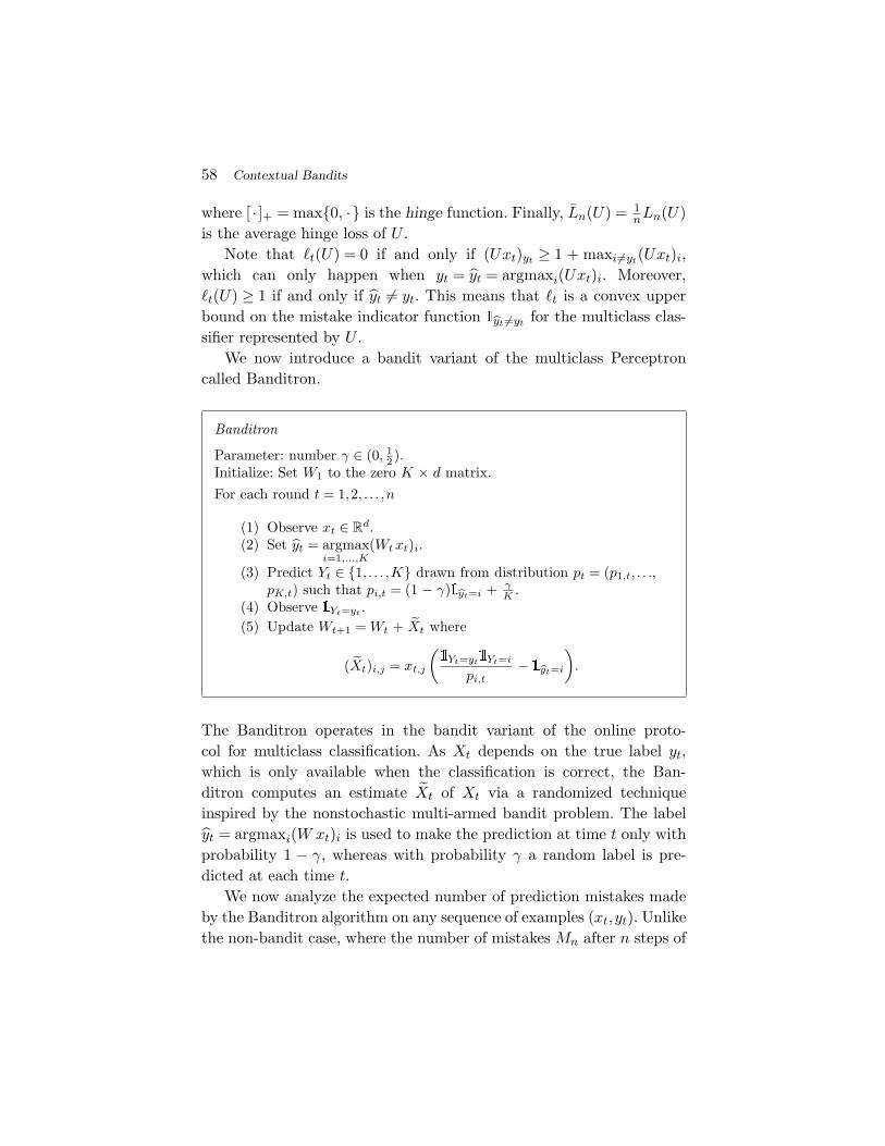
58 Contextual Bandits
where [ · ]+ = max0, · is the hinge function. Finally, Ln(U) = 1nLn(U)
is the average hinge loss of U .Note that t(U) = 0 if and only if (Uxt)yt ≥ 1 + maxi=yt(Uxt)i,
which can only happen when yt = yt = argmaxi(Uxt)i. Moreover,t(U) ≥ 1 if and only if yt = yt. This means that t is a convex upperbound on the mistake indicator function yt =yt
for the multiclass clas-sifier represented by U .
We now introduce a bandit variant of the multiclass Perceptroncalled Banditron.
Banditron
Parameter: number γ ∈ (0, 12 ).
Initialize: Set W1 to the zero K × d matrix.For each round t = 1,2, . . . ,n
(1) Observe xt ∈ Rd.
(2) Set yt = argmaxi=1,...,K
(Wtxt)i.
(3) Predict Yt ∈ 1, . . . ,K drawn from distribution pt = (p1,t, . . .,pK,t) such that pi,t = (1 − γ) yt=i + γ
K .(4) Observe Yt=yt .(5) Update Wt+1 = Wt + Xt where
(Xt)i,j = xt,j
(Yt=yt Yt=i
pi,t− yt=i
).
The Banditron operates in the bandit variant of the online proto-col for multiclass classification. As Xt depends on the true label yt,which is only available when the classification is correct, the Ban-ditron computes an estimate Xt of Xt via a randomized techniqueinspired by the nonstochastic multi-armed bandit problem. The labelyt = argmaxi(W xt)i is used to make the prediction at time t only withprobability 1 − γ, whereas with probability γ a random label is pre-dicted at each time t.
We now analyze the expected number of prediction mistakes madeby the Banditron algorithm on any sequence of examples (xt,yt). Unlikethe non-bandit case, where the number of mistakes Mn after n steps of
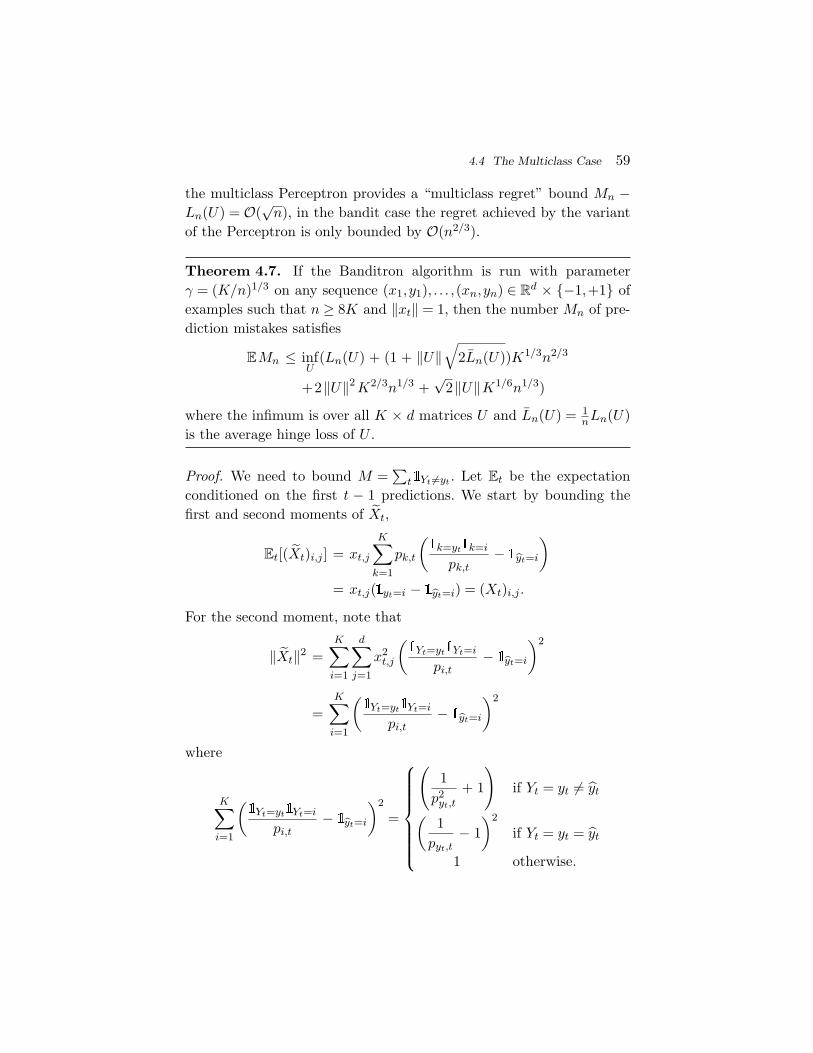
4.4 The Multiclass Case 59
the multiclass Perceptron provides a “multiclass regret” bound Mn −Ln(U) = O(
√n), in the bandit case the regret achieved by the variant
of the Perceptron is only bounded by O(n2/3).
Theorem 4.7. If the Banditron algorithm is run with parameterγ = (K/n)1/3 on any sequence (x1,y1), . . . ,(xn,yn) ∈ R
d × −1,+1 ofexamples such that n ≥ 8K and ‖xt‖ = 1, then the number Mn of pre-diction mistakes satisfies
EMn ≤ infU
(Ln(U) + (1 + ‖U‖√
2Ln(U))K1/3n2/3
+2‖U‖2K2/3n1/3 +√
2‖U‖K1/6n1/3)
where the infimum is over all K × d matrices U and Ln(U) = 1nLn(U)
is the average hinge loss of U .
Proof. We need to bound M =∑
t Yt =yt . Let Et be the expectationconditioned on the first t − 1 predictions. We start by bounding thefirst and second moments of Xt,
Et[(Xt)i,j ] = xt,j
K∑k=1
pk,t
(k=yt k=i
pk,t− yt=i
)= xt,j( yt=i − yt=i) = (Xt)i,j .
For the second moment, note that
‖Xt‖2 =K∑i=1
d∑j=1
x2t,j
(Yt=yt Yt=i
pi,t− yt=i
)2
=K∑i=1
(Yt=yt Yt=i
pi,t− yt=i
)2
where
K∑i=1
(Yt=yt Yt=i
pi,t− yt=i
)2
=
(1p2yt,t
+ 1
)if Yt = yt = yt(
1pyt,t
− 1)2
if Yt = yt = yt
1 otherwise.

60 Contextual Bandits
Therefore, if yt = yt,
Et‖Xt‖2 = pyt,t
(1p2yt,t
+ 1
)+ (1 − pyt,t)
= 1 +1py,t
= 1 +K
γ≤ 2K
γ
because pi,t = γ when yt = yt. Otherwise, if yt = yt
Et‖Xt‖2 = pyt,t
(1pyt,t
− 1)2
+ (1 − pyt,t)
=1pyt,t
− 1 =1
1 − γ − 1 ≤ 2γ
because pi,t = 1 − γ when yt = yt and γ ≤ 12 . Hence,
Et‖Xt‖2 ≤ 2(K
γyt =yt
+ γ yt=yt
).
We are now ready to prove a bound on the expected number of mis-takes. Following the standard analysis for the Perceptron algorithm,we derive upper and lower bounds on the expectation of the quantity⟨U,Wn+1
⟩= tr(UW
n+1), for an arbitrary K × d matrix U . First, usingCauchy–Schwartz and Jensen inequalities we obtain
E⟨U,Wn+1
⟩ ≤√‖U‖2 E‖Wn+1‖2.
Now
En[‖Wn+1‖2] = En[‖Wn‖2 + 2⟨Wn, Xn
⟩+ ‖Xn‖2]
≤ ‖Wn‖2 + En‖Xn‖2.
In order to see why the inequality holds, note that
En
⟨Wn, Xn
⟩=⟨Wn,Xn
⟩=
K∑i=1
(Wnxt)i( yn=i − yn=i)
= (Wnxn)yn − (Wnxn)yn≤ 0
4.4 The Multiclass Case 61
because yn = argmaxi=1,...,K(Wnxn)i by definition. Therefore, since W1
is the zero matrix,
E‖Wn+1‖2 ≤n∑t=1
E‖Xn‖2
≤ 2n∑t=1
(K
γP(yt = yt) + γP(yt = yt)
)
≤ 2Kγ
n∑t=1
P(yt = yt) + 2γn.
Thus we have
E⟨U,Wn+1
⟩ ≤ ‖U‖√√√√2K
γ
n∑t=1
P(yt = yt) + 2γn.
Now we lower bound⟨U,Wn+1
⟩as follows,
En
⟨U,Wn+1
⟩= En
⟨U,Wn + Xn
⟩=⟨U,Wn
⟩+⟨U,Xn
⟩≥ ⟨U,Wn
⟩+ yt =yt
− t(U)
because, by definition of t,
t(U) =[1 − (Uxt)yt + max
i=yt
(Uxt)i
]+
≥ 1 − (Uxt)yt + (Uxt)yt
≥ yt =yt− (Uxt)yt + (Uxt)yt
= yt =yt− ⟨U,Xt
⟩.
Therefore, using again the fact that W1 is the zero matrix,
E⟨U,Wn+1
⟩ ≥ n∑t=1
P(yt = yt) −n∑t=1
t(U).
Combining the upper and lower bounds on⟨U,Wn+1
⟩we get
n∑t=1
P(yt = yt) − Ln(U) ≤ ‖U‖√√√√2K
γ
n∑t=1
P(yt = yt) + 2γn.
62 Contextual Bandits
Solving for∑
tP(yt = yt) and overapproximating yields
n∑t=1
P(yt = yt) ≤ Ln(U) +2Kγ‖U‖2 + ‖U‖
√2KγLn(U) + 2γn
= Ln(U) +2Kγ‖U‖2 + ‖U‖
√(2KγLn(U) + 2γ
)n.
Now, since P(yt = Yt) = (1 − γ)P(yt = yt) + γ,
n∑t=1
P(yt = Yt) ≤ Ln(U) + γn +2Kγ‖U‖2
+ ‖U‖√(
2KγLn(U) + 2γ
)n.
Choosing γ as in the statement of the theorem yields the desired result.Note that γ ≤ 1
2 because we assume n ≥ 8K.
4.5 Bibliographic Remarks
A model of contextual stochastic bandits close to those studied here isintroduced by Wang et al. [166]. The context is provided by an i.i.d.sequence of random variables and the rewards for each arm dependon the context through an unknown parametric model belonging to aknown class. This result has been generalized to the non-i.i.d. case byWang et al. [165], to the multivariate linear case by Rusmevichientongand Tsitsiklis [148], and to the multivariate and nonparametric case byPerchet and Rigollet [143]. In Ref. [152], contexts and rewards belongto arbitrary metric spaces, and the unknown function mapping con-texts to rewards satisfies a Lipschitz assumption (remarkably, the samealgorithm also applies to slowly changing expected rewards and sleep-ing bandit settings). The case of deterministic covariates (fixed design),finitely many arms, and a linear stochastic dependence between covari-ates and rewards has been studied in [22, 66] — see also [2]. The workof Filippi et al. [78] extends the analysis of fixed design by assuminga generalized linear model to capture the dependence of rewards oncovariates.
4.5 Bibliographic Remarks 63
The simple contextual model analyzed in Section 4.1, as well asits extension described in Section 4.2.1, are due to Maillard andMunos [131]. The Exp4 algorithm for the adversarial case was intro-duced in Auer et al. [24]. Subsequent improvements were proposedin the two papers, i.e., Beygelzimer et al. [39] (Exp4.P with high-probability bounds) and McMahan and Streeter [136] (exploitation ofcorrelations in expert advice). The VE algorithm and its analysis inSection 4.3 are also taken from Beygelzimer et al. [39].
A stochastic model for contextual bandits with finitely many armsand finitely many states has been investigated by Seldin et al. [150]using new sophisticated tools of PAC-Bayesian analysis.
The general stochastic model of Section 4.3 for contextual banditswith finitely many arms is due to Langford and Zhang [126]. An efficientalgorithm for this model has been recently proposed in [74].
The bandit multiclass model of Section 4.4 is due to Langford andZhang [126]. The Banditron algorithm and its analysis are from Kakadeet al. [109]. See also [70, 97] for recent variants and improvements.

5Linear Bandits
We now consider the important generalization of adversarial banditswhere the set of arms 1, . . . ,K is replaced by a compact set K ⊂ R
d.In this case, the loss at each step is some function defined on K, andthe task is to pick an arm as close as possible to the minimum of theloss function at hand. In order to allow sublinear regret bounds, evenin the presence of infinitely many arms, we must assume some struc-ture for the loss function. In particular, in this section we assume thatthe loss at each time step is a linear function of arms. Linearity is astandard assumption (think, for instance, of linear regression) and nat-urally occurs in many bandit applications. The source routing problemmentioned in the Introduction is a good example, since the cost ofchoosing a routing path is linear in the cost of the edges that make upthe path. This defines the so-called online linear optimization setting:at each time step t = 1,2, . . . the forecaster chooses xt ∈ K while, simul-taneously, the adversary chooses t from some fixed and known subsetL of R
d. The loss incurred by the forecaster is the inner product xt t.
64
5.1 Exp2 (Expanded Exp) with John’s Exploration 65
In this section we focus on the analysis of the pseudo-regret
Rn = E
n∑t=1
xt t − min
x∈KE
n∑t=1
xt
where the expectation is with respect to the forecaster’s internal ran-domization. The adversarial bandit setting of Section 3 is obtained bychoosing K = e1, . . . ,ed, where e1, . . . ,ed is the canonical basis of R
d,and L = [0,1]d. Similarly to Section 3, we focus on the bandit feedbackwhere the forecaster only observes the incurred loss x
t t at the endround t. However, we also discuss the full information setting, wherethe complete loss vector t is revealed at the end of each round t, aswell as other feedback models.
It is important to note that, without any loss of generality (as faras regret bounds are concerned), one can always assume that K hassize O(nd). Indeed, since K is a compact set and the loss is linear (andtherefore Lipschitz), one can cover K with O(nd) points such that oneincurs a vanishing extra cumulative regret by playing on the discretiza-tion rather than on the original set. Of course, the downside of thisapproach is that a strategy resulting from such a cover is often notcomputationally efficient. On the other hand, this assumption allowsus to apply ideas from Section 3 to this more general setting. We ana-lyze the pseudo-regret for finite classes in Section 5.1. Without loss ofgenerality, it is also possible to assume that K is a convex set. Indeed,the pseudo-regret is the same if one plays xt, or if one plays a pointat random in K such that the expectation of the played point is xt.This remark is critical and allows us to develop a powerful technologyknown as the Mirror Descent algorithm. We describe this approach inSection 5.2 and explore it further in subsequent sections.
5.1 Exp2 (Expanded Exp) with John’s Exploration
In this section we work under the bounded scalar loss assumption. Thatis, we assume that K and L are such that |x| ≤ 1 for any (x,) ∈K × L. Moreover, we restrict our attention to finite sets K, with |K| =N . Without loss of generality we assume that K spans R
d. If it is not thecase, then one can rewrite the elements of K in some lower dimensional
66 Linear Bandits
vector space, and work there. Note that a trivial application of Exp3to the set K of arms gives a bound that scales as
√nN lnN . If K is a
discretized set (in the sense described earlier), then N is exponentialin d. We show here that, by appropriately modifying Exp3, one canobtain a polynomial regret of order
√nd lnN .
To describe the strategy, we first need a useful result from convexgeometry: John’s theorem. This result concerns the ellipsoid E of mini-mal volume enclosing a given convex set K (which we call John’s ellip-soid of K). Basically, the theorem states that E has many contact pointswith K, and these contact points are “nicely” distributed, in the sensethat they almost form an orthonormal basis — see [32] for a proof.
Theorem 5.1(John’s theorem). Let K ⊂ Rd be a convex set. If the
ellipsoid E of minimal volume enclosing K is the unit ball in somenorm derived from a scalar product 〈·, ·〉, then there exist M ≤ 1
2d(d +1) + 1 contact points u1, . . . ,uM between E and K, and a probabilitydistribution (µ1, . . . ,µM ) over these contact points, such that
x = d
M∑i=1
µi〈x,ui〉ui ∀x ∈ Rd.
In fact John’s theorem is an if and only if, but here we only needthe direction stated in the theorem. We are now in position to describethe strategy. Let Conv(S) be the convex hull of a set S ∈ R
d. First,we perform a preprocessing step in which the set K is rewritten sothat John’s ellipsoid of Conv(K) is the unit ball for some inner product〈·, ·〉. The loss of playing x ∈ K against ∈ L is then given by 〈x,〉.See [45] for the details of this transformation. Let u1, . . . ,uM ∈ K and(µ1, . . . ,µM ) satisfy Theorem 5.1 for the convex set Conv(K).
Recall from Section 3 that the key idea to play against an adversaryis to select xt at random from some probability distribution pt over K.We first describe how to build an unbiased estimate of t, given such apoint xt played at random from pt (such that pt(x) > 0 for any x ∈ K).Recall that the outer product x ⊗ x is defined as the linear mappingfrom R
d to Rd such that x ⊗ x(y) = 〈x,y〉x. Note that one can also view

5.1 Exp2 (Expanded Exp) with John’s Exploration 67
x ⊗ x as a d × d matrix, so that the evaluation of x ⊗ x is equivalentto a multiplication by the corresponding matrix. Now let
Pt =∑x∈K
pt(x)x ⊗ x.
Note that this matrix is invertible, since K is full rank and pt(x) > 0for all x ∈ K. The estimate for t is given by t = P−1
t (xt ⊗ xt)t. Notethat this is a valid estimate since (xt ⊗ xt)t = 〈xt, t〉xt and P−1
t areobserved quantities. Also, it is clearly an unbiased estimate.
Now the Exp2 algorithm with John’s exploration corresponds toplaying according to the following probability distribution
pt(x) = (1 − γ)exp(−η∑t−1
s=1〈x, t〉)
∑y∈K exp
(−η∑t−1
s=1〈y, t〉) + γ
M∑i=1
µi x=ui (5.1)
where η,γ > 0 are input parameters. Note that this corresponds toa variant of Exp3 using 〈x, t〉 as loss estimate for x ∈ K, and anexploration distribution supported by the contact points.
Theorem 5.2(Pseudo-regret of Exp2 with John’s exploration).For any η,γ > 0 such that ηd ≤ γ, Exp2 with John’s explorationsatisfies
Rn ≤ 2γn +lnNη
+ ηnd.
In particular, with η =√
lnN3nd and γ = ηd,
Rn ≤ 2√
3nd lnN.
Proof. Since K is finite, we can easily adapt the analysis of Exp3 inTheorem 3.1 to take into account the exploration term. This gives
Rn ≤ 2γn +lnNη
+ ηE
n∑t=1
∑x∈K
pt(x)〈x, t〉2

68 Linear Bandits
whenever η 〈x, t〉 ≤ 1 for all x ∈ K. We now bound the last term inthe right-hand side of the above inequality. Using the definition of theestimated loss t = P−1
t (xt ⊗ xt)t, we can write∑x∈K
pt(x)〈x, t〉2 =∑x∈K
pt(x)〈t,(x ⊗ x) t〉
= 〈t,Pt t〉= 〈xt, t〉2〈P−1
t xt,PtP−1t xt〉
≤ 〈P−1t xt,xt〉.
Now we use a spectral decomposition of Pt in an orthonormal basisfor 〈·, ·〉 and write Pt =
∑di=1λivi ⊗ vi. In particular, we have P−1
t =∑di=1
1λivi ⊗ vi and thus
E〈P−1t xt,xt〉 =
d∑i=1
1λi
E〈(vi ⊗ vi)xt,xt〉
=d∑i=1
1λi
E〈(xt ⊗ xt)vi,vi〉
=d∑i=1
1λi〈Pt vi,vi〉
=d∑i=1
1λi〈λivi,vi〉 = d.
Finally, to show η 〈x, t〉 ≤ 1 observe that
〈x, t〉 = 〈xt, t〉〈x,P−1t xt〉 ≤ 〈x,P−1
t xt〉 ≤ 1min1≤i≤dλi
,
where the last inequality follows from the fact that 〈x,x〉 ≤ 1 for anyx ∈ K, since K is included in the unit ball. To conclude the proof, weneed to lower bound the smallest eigenvalue of Pt. Using Theorem 5.1,one can see that Pt γ
dId, and thus λi ≥ γd . Since ηd ≤ γ, the proof is
concluded.
5.2 Online Mirror Descent (OMD) 69
5.2 Online Mirror Descent (OMD)
We now introduce the Online Mirror Descent (OMD) algorithm, apowerful generalization of gradient descent for sequential decisionproblems. We start by describing OMD for convex losses in the fullinformation setting. That is, L is a set of convex functions, and at theend of round t the forecaster observes t ∈ L rather than only t(xt).
The rest of this section is organized as follows. Next, we briefly recalla few key concepts from convex analysis. Then we describe the OMDstrategy and prove a general regret bound. In Section 5.3 we introduceOnline Stochastic Mirror Descent (OMSD), which is a variant of OMDbased on a stochastic estimate of the gradient. We apply this strategyto linear losses in two different bandit settings. Finally, in Section 5.5we show how OMSD obtains improved bounds in certain special cases.The case of convex losses with bandit feedback is treated in Section 6.
We introduce the following definitions.
Definition 5.1. Let X ⊆ Rd. A function f : X → R is subdifferentiable
if for all x ∈ X there exists g ∈ Rd such that
f(x) − f(y) ≤ g(x − y) ∀y ∈ X .Such a g is called a subgradient of f at x.
Abusing notation, we use ∇f(x) to denote both the gradient of fat x when f is differentiable and any subgradient of f at x when f issubdifferentiable (a sufficient condition for subdifferentiability of f isthat f is convex and X is open).
Definition 5.2. Let f : X → R be a convex function defined on a con-vex set X ⊆ R
d. The Legendre–Fenchel transform of f is defined by:
f∗(u) = supx∈X
(xu − f(x)).
This definition directly implies the Fenchel–Young inequality forconvex functions, ux ≤ f(x) + f∗(u).
Let D ⊂ Rd be an open convex set, and let D be the closure of D.
70 Linear Bandits
Definition 5.3. A continuous function F : D → R is Legendre if
(i) F is strictly convex and admits continuous first partialderivatives on D;
(ii) limx→D\D
‖∇F (x)‖ = +∞.1
The Bregman divergence DF : D × D → R associated with aLegendre function F is defined by DF (x,y) = F (x) − F (y) − (x − y)
∇F (y). Moreover, we say thatD∗ =∇F (D) is the dual space ofD underF . Note that, by definition, DF (x,y) > 0 if x = y, and DF (x,x) = 0.The following lemma is the key to understand how a Legendre functionacts on the space. See [61, Proposition 11.1] for a proof.
Lemma 5.3. Let F be a Legendre function. Then F ∗∗ = F , and∇F ∗ = (∇F )−1 restricted on the set D∗. Moreover, for all x,y ∈ D,
DF (x,y) = DF ∗(∇F (y),∇F (x)). (5.2)
The gradient ∇F maps D to the dual space D∗, and ∇F ∗ is theinverse mapping from the dual space to the original (primal) space.Note also that Equation (5.2) shows that the Bregman divergence in theprimal exactly corresponds to the Bregman divergence of the Legendretransform in the dual.
The next lemma shows that the geometry induced by a Bregmandivergence resembles to the geometry of the squared Euclidean dis-tance. See [61, Lemma 11.3] for a proof.
Lemma 5.4 (Generalized Pythagorean inequality). Let K ⊆ Dbe a closed convex set such that K ∩ D = ∅. Then, for all x ∈ D, theBregman projection
z = argminy∈K
DF (y,x)
1 By the equivalence of norms in Rd, this definition does not depend on the choice of thenorm.

5.2 Online Mirror Descent (OMD) 71
exists and is unique. Moreover, for all z ∈ K ∩ D and y ∈ K,
DF (y,x) ≥ DF (y,z) + DF (z,x).
The idea of OMD is very simple: first, select a Legendre function Fon D ⊃ K (such that K ∩ D = ∅); second, perform a gradient descentstep, where the update with the gradient is performed in the dual spaceD∗ rather than in the primal D; and third, project back to K accordingto the Bregman divergence defined by F .
OMD (Online Mirror Descent):
Parameters: compact and convex set K ⊆ Rd, learning rate η > 0,
Legendre function F on D ⊃ K.Initialize: x1 ∈ argmin
x∈KF (x) (note that x1 ∈ K ∩ D).
For each round t = 1,2, . . . ,n
(1) Play xt and observe loss vector t.(2) wt+1 =∇F ∗(∇F (xt) − η∇t(xt)).(3) xt+1 = argmin
y∈KDF (y,wt+1).
Note that step (2) is well defined if the following consistency condi-tion is satisfied:
∇F (x) − η∇(x) ∈ D∗ ∀(x,) ∈ (K ∩ D) × L. (5.3)
Note also that step (2) can be rewritten as
∇F (wt+1) =∇F (xt) − η∇t(xt). (5.4)
Finally, note that the Bregman projection in step (3) is a convex pro-gram, in the sense that x → DF (x,y) is always a convex function. Thisdoes not necessarily imply that step (3) can be performed efficiently,since in some cases the feasible set K might only be described with anexponential number of constraints (we encounter examples like this inSection 5.4).
In the description above we emphasized that F has to be a Legendrefunction. In fact, as we see in Theorem 5.6, if F has effective domain
72 Linear Bandits
K (that is, F takes value +∞ outside of K), then it suffices that theLegendre–Fenchel dual F ∗ is differentiable on R
d to obtain a good regretbound. See the end of this section for more details on this.
When K is the simplex and F (x) =∑d
i=1xi lnxi −∑d
i=1xi, OMDreduces to an exponentially weighted average forecaster, similar tothose studied in Section 3. The well-known online gradient descentstrategy corresponds to taking F (x) = 1
2 ‖x‖22. In the following we shallsee other possibilities for the Legendre function F .
We prove now a very general and powerful theorem concerning theregret of OMD.
Theorem 5.5 (Regret of OMD with a Legendre function). LetK be a compact and convex set of arms, L be a set of subdifferentiablefunctions, and F a Legendre function defined on D ⊃ K, such thatEquation (5.3) is satisfied. Then OMD satisfies for any x ∈ K,
n∑t=1
t(xt) −n∑t=1
t(x) ≤ F (x) − F (x1)η
+1η
n∑t=1
DF ∗(∇F (xt) − η∇t(xt),∇F (xt)).
Proof. Let x ∈ K. Since L is a set of subdifferentiable functions, wehave:
n∑t=1
(t(xt) − t(x)) ≤n∑t=1
∇t(xt)(xt − x).
Using Equation (5.4), and applying the definition of DF , one obtains
η∇t(xt)(xt − x) = (x − xt)(∇F (wt+1) − ∇F (xt))
= DF (x,xt) + DF (xt,wt+1) − DF (x,wt+1).
By Lemma 5.4, one gets DF (x,wt+1) ≥ DF (x,xt+1) + DF (xt+1,wt+1),hence
η∇t(xt)(xt − x) ≤ DF (x,xt) + DF (xt,wt+1)
−DF (x,xt+1) − DF (xt+1,wt+1).
5.2 Online Mirror Descent (OMD) 73
Summing over t then givesn∑t=1
η∇t(xt)(xt − x) ≤ DF (x,x1) − DF (x,xn+1)
+n∑t=1
(DF (xt,wt+1) − DF (xt+1,wt+1)).
By the nonnegativity of the Bregman divergences, we getn∑t=1
η∇t(xt)(xt − x) ≤ DF (x,x1) +n∑t=1
DF (xt,wt+1).
From Equation (5.2), one has DF (xt,wt+1) = DF ∗(∇F (xt) −η∇t(xt),∇F (at)) and, moreover, by first-order optimality, onehas DF (x,x1) ≤ F (x) − F (x1), which concludes the proof.
We show now how to prove a regret bound if F has effective domainK and F ∗ is differentiable on R
d, but not necessarily Legendre. In thiscase, it is easy to see that step (1) and step (2) in OMD reduce to
xt+1 =∇F ∗(−η
t−1∑s=1
∇s(xs)).
Theorem 5.6 (Regret of OMD with non-Legendre function).Let K be a compact set of actions, L be a set of subdifferentiablefunctions, and F a function with effective domain K such that F ∗ isdifferentiable on R
d. Then for any x ∈ K OMD satisfiesn∑t=1
t(xt) −n∑t=1
t(x) ≤ F (x) − F (x1)η
+1η
n∑t=1
DF ∗
(−η
t∑s=1
∇s(xs),−ηt−1∑s=1
∇s(xs)).
Proof. Let x ∈ K. Since L is a set of subdifferentiable functions, wehave
n∑t=1
(t(xt) − t(x)) ≤n∑t=1
∇t(xt)(xt − x).

74 Linear Bandits
Using the Fenchel–Young inequality, one obtains
−ηn∑t=1
∇t(xt)x
≤ F (x) + F ∗(−η
n∑t=1
∇t(xt))
= F (a) + F ∗(0)
+n∑t=1
(F ∗(−η
t∑s=1
∇s(xs))− F ∗
(−η
t−1∑s=1
∇s(xs)))
.
Observe that F ∗(0) = −F (x1) and, for each term in the above sum,
∇F ∗(−η
t−1∑s=1
∇s(xs))
(−η∇t(xt))
+DF ∗
(−η
t∑s=1
∇s(xs),−ηt−1∑s=1
∇s(xs))
= −ηxt ∇t(xt) + DF ∗
(−η
t∑s=1
∇s(xs),−ηt−1∑s=1
∇s(xs)).
5.3 Online Stochastic Mirror Descent (OSMD)
We now turn to the analysis of the bandit setting, where the gradientinformation ∇t(xt) is not available, and thus one cannot run OMD.This scenario has been extensively in gradient-free optimization, andthe basic idea is to play a perturbed version xt of the current point xt.This should be done in such a way that, upon observing t(xt), one canbuild an unbiased estimate gt of ∇t(xt). Whereas such estimators arepresented in Section 6, here we restrict our attention to linear losses.For this simpler case we consider specialized estimators with optimalperformances. Given a perturbation scheme, one can run OMD withthe gradient estimates instead of the true gradients. We call OnlineStochastic Mirror Descent (OSMD) the resulting algorithm.

5.3 Online Stochastic Mirror Descent (OSMD) 75
OSMD (Online Stochastic Mirror Descent):Parameters: compact and convex set K ⊆ R
d, learning rate η > 0, Legen-dre function F on D ⊃ K.Initialize: x1 ∈ argmin
x∈KF (x) (note that x1 ∈ K ∩ D).
For each round t = 1,2, . . . ,n
(1) Play a random perturbation xt of xt and observe t(xt)(2) Compute random estimate gt of ∇t(xt)(3) wt+1 =∇F ∗(∇F (xt) − ηgt)(4) xt+1 = argmin
y∈KDF (y,wt+1)
In order to relate this linear bandit strategy to the Exp2 forecaster(Equation (5.1)), it is important to observe that running the Exp2forecaster over a finite set K of arms, with exploration distributionµ and mixing coefficient γ > 0, is equivalent to running OSMD overthe |K|-dimensional simplex with F (x) = 1
η
∑x∈Kx lnx (the negative
entropy), xt drawn from (1 − γ)xt + γµ, and estimated linear loss gt =(〈x, t〉)x∈K. Indeed, the projection step (4), when F is the negativeentropy, corresponds to the standard normalization of a probabilitydistribution.
The following theorem establishes a general regret bound for OSMD.Note that here the pseudo-regret is defined as
Rn = E
n∑t=1
t(xt) − minx∈K
E
n∑t=1
t(x).
Note also that we state the theorem for a Legendre function F , but asimilar result can be obtained under the same assumptions as those ofTheorem 5.6.
Theorem 5.7(Pseudo-regret of OSMD). Let K be a compact andconvex set, L a set of subdifferentiable functions, and F a Legendrefunction defined on D ⊃ K. If OSMD is run with a loss estimate gtsuch that Equation (5.3) is satisfied (with ∇(x) replaced by gt), and

76 Linear Bandits
with E[gt | xt] =∇t(xt), then
Rn ≤ supx∈KF (x) − F (x1)η
+1η
n∑t=1
EDF ∗(∇F (xt) − ηgt,∇F (xt))
+n∑t=1
E[‖xt − xt‖‖gt‖∗]
for any norm ‖·‖. Moreover if the loss is linear, that is (x) = x, then
Rn ≤ supx∈KF (x) − F (x1)η
+1η
n∑t=1
EDF ∗(∇F (xt) − ηgt,∇F (xt))
+n∑t=1
E[‖xt − E[xt | xt]‖‖gt‖∗].
Proof. Using Theorem 5.5 one directly obtains:n∑t=1
gt (xt − x) ≤ F (x) − F (x1)
η+
1η
n∑t=1
EDF ∗(∇F (xt) − ηgt,∇F (xt)).
Moreover since E[gt | xt] =∇t(xt), one has:
E
n∑t=1
(t(xt) − t(x)) = E
n∑t=1
(t(xt) − t(xt) + t(xt) − t(x))
≤ E
n∑t=1
‖xt − xt‖‖gt‖∗ + E
n∑t=1
∇t(xt)(xt − x)
= E
n∑t=1
‖xt − xt‖‖gt‖∗ + E
n∑t=1
gt (xt − x)
which concludes the proof of the first regret bound. The case of a linearloss follows very easily from the same computations.
5.4 Online Combinatorial Optimization
In this section we consider an interesting special case of online linearoptimization. In the online combinatorial optimization setting the set ofarms is C ⊆ 0,1d and the set of linear loss functions is L = [0,1]d. We
5.4 Online Combinatorial Optimization 77
assume ‖v‖1 = m for all v ∈ C and for some integer m ≤ d. Many inter-esting problems fall into this framework, including ranking/selection ofm items, or path planning.
Here we focus on the version of the problem with semi-bandit feed-back, which is defined as follows: after playing vt ∈ C, one observes(t(1)vt(1), . . . , t(d)vt(d)). Namely, one only observes the coordinatesof the loss that were active in the arm vt that we chose. This settinghas thus a much weaker feedback than the full information case, butstill stronger than the bandit case. Note that the semi-bandit settingincludes the basic multi-armed bandit problem of Section 3, whichsimply corresponds to C = e1, . . . ,ed where e1, . . . ,ed is the canonicalbasis of R
d.Again, the key to tackle this kind of problem is to select vt at random
from some probability distribution pt over C. Note that such a probabil-ity corresponds to an average point xt ∈ Conv(C). Turning the tables,one can view vt as a random perturbation of xt such that E[vt | xt] = xt.This suggests a strategy: play OSMD on K = Conv(C), with xt = vt.Surprisingly, we show that this randomization is enough to obtain agood unbiased estimate of the loss, and that it is not necessary to addfurther perturbations to xt. Note that E[xt | xt] = xt by definition. Wenow need to describe how to obtain an unbiased estimate of the gradi-ent (which is the loss vector itself, since losses are linear). The followingsimple formula gives an unbiased estimate of the loss:
t(i) =t(i)vt(i)xt(i)
∀ i ∈ 1, . . . ,d. (5.5)
Note that this is a valid estimate since it only makes the use of(t(1)vt(1), . . . , t(d)vt(d)). Moreover, it is unbiased with respect to therandom drawing of vt from pt. Indeed,
E[t(i) | xt] =t(i)xt(i)
E[vt(i) | xt] = t(i).
Using Theorem 5.7 one directly obtains:
Rn ≤ supx∈KF (x) − F (x1)η
+1η
n∑t=1
EDF ∗(∇F (xt) − ηt,∇F (xt)). (5.6)

78 Linear Bandits
We show now how to use this bound to obtain concrete performancesfor OSMD using the negative entropy as Legendre function. Later, weshow that one can improve the results by logarithmic factors, using amore subtle Legendre function.
We start with OSMD and the negative entropy.
Theorem 5.8 (OSMD with negative entropy). For any set C ⊆0,1d, if OSMD is run on K = Conv(C) with F (x) =
∑di=1xi lnxi −∑d
i=1xi, perturbed points xt such that E[xt | xt] = xt, and loss esti-mates t, then
Rn ≤ m
ηlnd
m+η
2
n∑t=1
d∑i=1
E[xt(i) t(i)2].
In particular, with the estimate (Equation (5.5)) and η =√
2mnd ln d
m ,
Rn ≤√
2mdn lnd
m.
Proof. First note that:
F (x) − F (x1) ≤d∑i=1
x1(i) ln1
x1(i)≤m ln
(d∑i=1
x1(i)m
1x1(i)
)= m ln
d
m.
Moreover, straightforward computations give
DF ∗(∇F (xt) − ηt,∇F (xt)) =d∑i=1
xt(i)Θ(−ηt(i))
where Θ : x ∈ R → exp(x) − 1 − x. Using that Θ(x) ≤ x2
2 for all x ≤ 0,concludes the proof of the first inequality (since t(i) ≥ 0). The secondinequality follows from
xt(i)E[t(i)2 | xt] = xt(i)t(i)2
xt(i)2E[vt(i) | xt] ≤ 1
where we used t(i) ∈ [0,1] and vt(i) ∈ 0,1.

5.4 Online Combinatorial Optimization 79
We now greatly generalize the negative entropy with the followingdefinition. When used with OSMD, this more general entropy allowsus to obtain a bound tighter than that of Theorem 5.8.
Definition 5.4. Let ω ≥ 0. A function ψ : (−∞,a)→ R∗+ for some
a ∈ R ∪ +∞ is called an ω-potential if it is convex, continuously dif-ferentiable, and satisfies
limx→−∞ψ(x) = ω lim
x→aψ(x) = +∞
ψ′ > 0∫ ω+1
ω|ψ−1(s)|ds < +∞.
With a potential ψ we associate the function Fψ defined on D =(ω,+∞)d by
Fψ(x) =d∑i=1
∫ xi
ωψ−1(s)ds.
We restrict our attention to 0-potentials. A nonzero ω might beused to derive high probability regret bounds (instead of pseudo-regretbounds). Note that with ψ(x) = ex we have that Fψ reduces to thenegative entropy.
Lemma 5.9. Let ψ be a 0-potential. Then Fψ is Legendre and for allu,v ∈ D∗ = (−∞,a)d such that ui ≤ vi for i = 1, . . . ,d,
DF ∗(u,v) ≤ 12
d∑i=1
ψ′(vi)(ui − vi)2.
Proof. It is easy to check that F is a Legendre function. Moreover,since ∇F ∗(u) = (∇F )−1(u) = (ψ(u1), . . . ,ψ(ud)) we obtain
DF ∗(u,v) =d∑i=1
(∫ ui
vi
ψ(s)ds − (ui − vi)ψ(vi)).

80 Linear Bandits
From a Taylor expansion, we have
DF ∗(u,v) ≤d∑i=1
maxs∈[ui,vi]
12ψ′(s)(ui − vi)2.
Since the function ψ is convex, and ui ≤ vi, we have
maxs∈[ui,vi]
ψ′(s) ≤ ψ′(maxui,vi) ≤ ψ′(vi)
which gives the desired result.
We are now ready to bound the pseudo-regret of OSMD run with anarbitrary 0-potential. For a specific choice of the potential we obtainan improvement of Theorem 5.8. In particular for m = 1 this resultgives the log-free bound for the adversarial multi-armed bandit thatwas discussed in Section 3.4.1.
Theorem 5.10 (OSMD with a 0-potential). For any set subsetC of 0,1d, if OSMD is run on K = Conv(C) with Fψ defined by a0-potential ψ, and nonnegative loss estimates t, then
Rn ≤ supx∈KFψ(x) − Fψ(x1)η
+η
2
n∑t=1
d∑i=1
E
[t(i)2
(ψ−1)′(xt(i))
].
In particular, choosing the 0-potential ψ(x) = (−x)−q, the estimate
(Equation (5.5)), and η =√
2q−1
m1−2/q
d1−2/q ,
Rn ≤ q√
2q − 1
mdn.
With q = 2 this gives
Rn ≤ 2√
2mdn.
Proof. First note that since D∗ = (−∞,a)d and t has nonnegativecoordinates, then Equation (5.3) is satisfied and thus OSMD is welldefined.
5.5 Improved Regret Bounds for Bandit Feedback 81
The first inequality trivially follows from Equation (5.6),Lemma 5.9, and the fact that ψ′(ψ−1(s)) = 1
(ψ−1)′(s) .
Let ψ(x) = (−x)−q. Then we have that ψ−1(x) = −x−1/q andF (x) = − q
q−1∑d
i=1x1−1/qi . In particular, by Holder’s inequality, since∑d
i=1x1(i) = m,
F (x) − F (x1) ≤ q
q − 1
d∑i=1
x1(i)1−1/q ≤ q
q − 1m(q−1)/qd1/q.
Moreover, note that (ψ−1)′(x) = 1qx
−1−1/q, and
d∑i=1
E
[t(i)2
(ψ−1)′(xt(i))
∣∣∣∣∣xt]≤ q
d∑i=1
xt(i)1/q ≤ qm1/qd1−1/q
which ends the proof.
5.5 Improved Regret Bounds for Bandit Feedback
We go back to the setting of linear losses with bandit feedback consid-ered in Section 5.1. Namely, actions belong to a compact and convex setK ⊆ R
d, losses belong to a subset L ⊆ Rd, and the loss of playing xt ∈ K
at time t is xt t, which is also the feedback received by the player. As
we proved in Section 5.1, under the bounded scalar loss assumption,|x| ≤ 1 for all (x,) ∈ K × L, one can obtain a regret bound of orderd√n (up to logarithmic factors) for any compact and convex set K.
It can be shown that this rate is not improvable in general. However,results from Section 5.4 (or from Section 3) show that for the simplex,one can obtain a regret bound of order
√dn, and we showed in Sec-
tion 3 that this rate is also unimprovable. The problem of obtaininga characterization of the sets for which such improved regret boundsare possible is an open problem. Improved rates can be obtained foranother convex body: the Euclidean ball. We now describe a strategythat attains a pseudo-regret of order
√dn (up to a logarithmic factor)
in this case. The strategy is based on OSMD with a carefully chosenLegendre function.
In the following, let ‖·‖ be the Euclidean norm. We considerthe online linear optimization problem with bandit feedback on the
82 Linear Bandits
Euclidean unit ball K = x ∈ Rd : ‖x‖ ≤ 1. We perform the following
perturbation of a point xt in the interior of K,
xt =xt/‖xt‖ if ξt = 1,εt eIt otherwise
where ξt is a Bernoulli random variable of parameter ‖xt‖, It is drawnuniformly at random in 1, . . . ,d, and εt is a Rademacher randomvariable with parameter 1
2 .It is easy to check that this perturbation is unbiased, in the sense
that E[xt | xt] = xt. An unbiased estimate of the loss vector is given by
t = d(1 − ξt) xt t
1 − ‖xt‖ xt. (5.7)
Again, it is easy to check that E[t | xt] = xt. We are now ready to provethe following result, showing that OSMD with a suitable F achieves apseudo-regret of order
√dn lnn on the Euclidean ball.
Theorem 5.11(OSMD for the Euclidean ball). LetK = L = x ∈Rd : ‖x‖ ≤ 1 define an online linear optimization problem with ban-
dit feedback. If OSMD is run on K′ = (1 − γ)K with F (x) = − ln(1 −‖x‖) − ‖x‖ and the estimate (Equation (5.7)), then for any η > 0 suchthat ηd ≤ 1
2 ,
Rn ≤ γn +lnγ−1
η+ η
n∑t=1
E[(1 − ‖xt‖)‖t‖2]. (5.8)
In particular, with γ = 1√n
and η =√
lnn2nd ,
Rn ≤ 3√dn lnn. (5.9)
Proof. First, it is clear that by playing on K′ = (1 − γ)K instead of K,OSMD incurs an extra γn regret. Second, note that F is stricly convex(it is the composition of a convex and nondecreasing function with theEuclidean norm) and
∇F (x) =x
1 − ‖x‖ . (5.10)

5.5 Improved Regret Bounds for Bandit Feedback 83
In particular, F is Legendre on the open unit ball D = x ∈ Rd :
‖x‖ < 1, and one has D∗ = Rd. Hence Equation (5.3) is always sat-
isfied and OSMD is well defined. Now the regret with respect to K′ canbe bounded as follows: using Theorem 5.7 and the unbiasedness of xtand t we get
supx∈KF (x) − F (x1)η
+1η
n∑t=1
EDF ∗(∇F (xt) − ηt,∇F (xt)).
The first term is clearly bounded by 1η ln 1
γ (since x1 = 0). For the secondterm, we need to do a few computations. The first one follows fromEquation (5.10), the others follow from simple algebra
∇F ∗(u) =u
1 + ‖u‖F ∗(u) = − ln(1 + ‖u‖) + ‖u‖
DF ∗(u,v) =1
1 + ‖v‖(‖u‖ − ‖v‖ + ‖u‖ · ‖v‖ − vTu
−(1 + ‖v‖) ln(
1 +‖u‖ − ‖v‖1 + ‖v‖
)).
Let Θ(u,v) such that DF ∗(u,v) = 11+‖v‖Θ(u,v). First note that
11 + ‖∇F (xt)‖ = 1 − ‖xt‖ . (5.11)
Thus, in order to prove Equation (5.8) it remains to show that Θ(u,v) ≤‖u − v‖2, for u =∇F (xt) − ηt and v =∇F (xt). In fact, we prove thatthis inequality holds as soon as ‖u‖−‖v‖
1+‖v‖ ≥ −12 . This is the case for the
pair (u,v) under consideration, since by the triangle inequality, Equa-tions (5.7) and (5.11), and the assumption on η,
‖u‖ − ‖v‖1 + ‖v‖ ≥ −
η‖t‖1 + ‖v‖ ≥ −ηd ≥ −
12.
Now using that ln(1 + x) ≥ x − x2 for all x ≥ −12 , we obtain that for
u,v such that ‖u‖−‖v‖1+‖v‖ ≥ −1
2 ,
Θ(u,v) ≤ (‖u‖ − ‖v‖)21 + ‖v‖ + ‖u‖ · ‖v‖ − vu
≤ (‖u‖ − ‖v‖)2 + ‖u‖ · ‖v‖ − vu
84 Linear Bandits
= ‖u‖2 + ‖v‖2 − ‖u‖ · ‖v‖ − vu
= ‖u − v‖2 + 2vu − ‖u‖ · ‖v‖ − vu
≤ ‖u − v‖2
which concludes the proof of Equation (5.8). For the proof of Equa-tion (5.9) it suffices to note that
E[1 − ‖xt‖‖t‖2] = (1 − ‖xt‖)d∑i=1
1 − ‖xt‖d
d2
(1 − ‖xt‖)2 (t ei)2
= d‖t‖2≤ d
and perform with straightforward computations.
5.6 Refinements and Bibliographic Remarks
Online convex optimization in the full information settingwas introducedby Zinkevich [175]. Online linear optimization with bandit feedback waspioneered in [27, 135]. For this problem, Dani et al. [71] were the firstto obtain optimal O(
√n) bounds in terms of the number n of rounds.
This was done using the Exp2 strategy with an exploration uniform overa barycentric spanner for K. The exploration part was first improvedby Cesa-Bianchi and Lugosi [62] for combinatorial sets K. Finally, theoptimal exploration based on John’s theorem was introduced by Bubecket al. [45]. Theorem 5.2 is extracted from this last paper.
Simultaneously with the line of research on Exp2, algorithms basedon Online Mirror Descent were also investigated. Mirror Descent wasoriginally introduced in the seminal work of Nemirovski [137] andNemirovski and Yudin [139] as a standard (offline) convex optimiza-tion method. A somewhat similar class of algorithms was rediscoveredin the online learning community, see [88, 101, 119, 151]. The connec-tion between existing online learning algorithms (such as Exponentialweights or Online Gradient Descent) and Mirror Descent was first madeexplicit in [61] — see also [145] and [95]. Earlier applications of MirrorDescent in the learning community can be found in [106]. The firstapplication of Mirror Descent to online linear optimization with bandit

5.6 Refinements and Bibliographic Remarks 85
feedback was given by Abernethy et al. [3]. In this pioneering paper, theauthors describe the first computationally efficient strategy (i.e., withcomplexity polynomial in d) with O(
√n) regret. The main idea is to use
Mirror Descent with a self-concordant barrier F for the set K. Unfor-tunately, the drawback is a suboptimal dependency on d in the regret.More precisely. they obtain a O(d2√n) regret under the bounded scalarloss assumption, while Exp2 with John’s exploration attains O(d
√n).
However, Mirror Descent can also deliver optimal regret bounds in thebandit case, as we showed in Section 5.5, which is extracted from [45].
The presentation of the Online Mirror Descent algorithm inSection 5.2 is inspired by Bubeck [44]. The definition of Legendrefunctions comes from [61, Section 11] — further developments on convexanalysis can be found in [42, 102]. Theorem 5.5 is taken from Audibertet al. [19], but the proof technique goes back at least to Ben-Tal andNemirovski [37]. The proof of Theorem 5.6 is adapted from Kakadeet al. [107]. Section 5.3 is inspired by gradient-free optimization, a topicextensively studied since [118, 147] — see [31, 67, 138, 140] for recentaccounts on this theory. Alternative views have been proposed on theOnline Mirror Descent strategy. In particular, it is equivalent to a FollowThe Regularized Leader, and to proximal algorithms, see Rakhlin [145].This viewpoint was pioneered by Beck and Teboulle [36] — see also [35]formore details. Finally, a notion of universality ofOnlineMirrorDescentin the online prediction setting was proposed by Srebro et al. [154].
The online combinatorial optimization problem studied inSection 5.4 was introduced by Kalai and Vempala [110] for the full infor-mation setting. Several works have studied this problem for specific setsC, see in particular [62, 98, 100, 124, 159, 168, 169]. The semi-banditfeedback was studied in the series of papers [19, 91, 111, 163]. The pre-sentation adopted in this section is based on the last paper. OSMD withnegative entropy was first studied by Helmbold and Warmuth [100] forthe full information setting and for a specific set C. It was then studiedmore generally in [124] for any set C. The generalization to semi-banditfeedback was done by Audibert et al. [19]. OSMD with a Legendrederived from a potential was introduced by Audibert et al. [19]. In thecase of the simplex, this strategy corresponds to the INF strategy ofAudibert and Bubeck [17] discussed in Section 3.4.1.

86 Linear Bandits
Online linear optimization is still far from being completely under-stood. For instance, see [44, Section 9] for a list of open problems. Inthis section we also omitted a few important topics related to onlinelinear optimization. We briefly review some of them below.
5.6.1 Lower Bounds
Under the bounded scalar loss assumption, it was proved by Daniet al. [71] that for K = [−1,1]d the minimax regret in the full infor-mation setting is at least of order
√dn, while under bandit feedback
it is of order d√n. In both cases Exp2 is matching these lower bounds
(using John’s exploration in the bandit case).In the combinatorial setting, where K ⊂ 0,1d and L = [0,1]d,
Audibert et al. [19] show that the minimax regret in the full informa-tion and semi-bandit cases is at least of order d
√n, while in the bandit
case it is of order d3/2√n. OSMD with the negative entropy matchesthe bounds in the full information and semi-bandit cases. However,in the bandit case the best-known bound is obtained by Exp2 (withJohn’s exploration) and gives a regret of order d2√n. It is importantto remark that Audibert et al. [19] show that Exp2 is a provably sub-optimal strategy in the combinatorial setting.
Finally, lower bounds for the full information case, and for a fewspecific sets K of interest, were derived by Koolen et al. [124].
5.6.2 High Probability Bounds
In this section we focused on the pseudo-regret Rn. However, just likein Section 3, a much more important and interesting statement con-cerns high probability bounds for the regret Rn. Partial results in thisdirection can be found in [33] for the Exp2 strategy, and in [4] for theOSMD algorithm.
5.6.3 Stochastic Online Linear Optimization
Similarly to the stochastic bandit case (see Section 2), a natural restric-tion to consider for the adversary is that the sequence of losses 1, 2, . . .

5.6 Refinements and Bibliographic Remarks 87
is an i.i.d. sequence. This stochastic setting was introduced by Auer [22],and further studied by Dani et al. [72]. In particular, in the latter paperit was proved that regrets logarithmic in n and polynomial in d are pos-sible, as long as K is a polytope. Recent progress on this problem canbe found in [1, 78, 148].

6Nonlinear Bandits
We now extend the analysis of the previous section to the followingscenario: arms are still points in a convex set K ⊂ R
d, but now lossesare not necessarily linear functions of the arms. More precisely theadversary selects loss functions from some set L of real-valued functionsdefined on K. The pseudo-regret is then defined as:
Rn = E
n∑t=1
t(xt) − minx∈K
E
n∑t=1
t(x).
This modification has important consequences. For instance withstrictly convex losses one has to do local perturbations in order toestimate the loss gradient, this is in contrast to the global perturba-tions studied in the previous section. In agreement with the settingof Section 5, we initially focus on the nonstochastic setting, wherethe forecaster faces an unknown sequence of convex Lipschitz anddifferentiable losses (in the nonlinear case the regret scales with theLipschitz constant of losses). Problems of this kind can be viewedas dynamic variants of convex optimization problems, in which the
88

6.1 Two-Point Bandit Feedback 89
convex function to optimize evolves over time. The bandit constraintcan be simply interpreted as the impossibility of computing gradients(because, for instance, we do not have an explicit representation of thefunction, but it can only be accessed by querying for values at desiredpoints).
We look at two feedback models. In the first one, at each step theforecaster evaluates the loss function at two points: the played pointplus an additional point of its choice. In the second one, only the value ofthe loss evaluated at the played point is made available to the forecaster.We show that while the two-point model allows for a O(
√n) bound on
pseudo-regret, in the one-point model a pseudo-regret bound of onlyO(n3/4) is achieved. The stochastic setting is investigated in Section 6.3where, similarly to Section 2, we assume that each play of an armreturns a stochastic loss with fixed but unknown mean. Unlike thenonstochastic case, the mean loss function is assumed to be Lipschitzand unimodal, but not necessarily convex. For keeping things simple,the stochastic setting is studied in one-dimensional case, when armsare points in the unit interval. For this case we show a bound on thepseudo-regret of O(
√n(logn)).
6.1 Two-Point Bandit Feedback
We start by analyzing the nonstochastic case in the two-point feed-back model: at each time step t, the forecaster observes the value ofa convex and differentiable loss function t at the played point xt andat an extra point x′
t of its choice. If the second point is chosen at ran-dom in a neighborhood of the first one, one can use it to computean estimate of the gradient of t at xt. Hence, running OSMD on theestimated gradients we obtain a regret bound controlled by the secondmoments of these estimates. The algorithm we present in this sectionfollows this intuition, although — for technical reasons — the gradientis estimated at a point which is close but distinct from the point actuallyplayed.
We focus our analysis on OSMD with Legendre function F = 12 ‖·‖2,
where ‖·‖ is the Euclidean norm. The resulting strategy, OSGD (OnlineStochastic Gradient Descent), is sketched below here.

90 Nonlinear Bandits
OSGD (Online Stochastic Gradient Descent):Parameters: Closed and convex set K ⊆ R
d, learning rate η > 0.Initialize: x1 = (0, . . . ,0).For each round t = 1,2, . . . ,n
(1) Observe stochastic estimate gt(xt) of ∇t(xt);(2) x′
t+1 = xt − η gt(xt);(3) xt+1 = argmin
y∈K
∥∥y − x′t+1
∥∥;
We now introduce our main technical tool: the two-point gradientestimate. The two points on which the loss value is queried at time t aredenoted by X+
t and X−t . OSGD always plays one of these two points
at random.Let B =
x ∈ R
d : ‖x‖ ≤ 1
be the unit ball in Rd and S =
x ∈ Rd : ‖x‖ = 1
be the unit sphere. Fix δ > 0 and introduce the
notations X+t = xt + δS and X−
t = xt − δS, where xt ∈ K and S is arandom variable with uniform distribution in S. Then, for any convexloss t, the two-point gradient estimate gt is defined by
gt(xt) =d
2δ(t(X+
t ) − t(X−t ))S. (6.1)
In order to compute the expectation of gt, first note that by symmetry
E gt(x) =d
δE[t(x + δS)S].
In order to compute the expectation in the right-hand side we need thefollowing preliminary lemma.
Lemma 6.1. For any differentiable function : Rd→ R
∇∫
B
(x + δb)db =∫
S
(x + δs)sdσ(s)
where σ is the unnormalized spherical measure.

6.1 Two-Point Bandit Feedback 91
Proof. The proof of this result is an easy consequence of the DivergenceTheorem,
∇∫
B
(x + δb)db =∫
B
∇(x + δb)db
=∫
S
1δ(x + δs)sdσ(s)
=1δ
∫S
(x + δs)sdσ(s).
We are now fully equipped to compute the expectation of gt.
Lemma 6.2. If B is a random variable with uniform distribution in B
and S is a random variable with uniform distribution in S, then for alldifferentiable functions t : R
d→ R,d
δE[(x + δS)S] =∇E(x + δB).
Proof. First consider the easy one-dimensional case. Namely, K = [a,b]for some reals a < b. Note that, in this case, S is uniform in −1,+1whereas B is uniform in [−1,+1]. Then
E(x + δB) =12δ
∫ δ
−δ(x + ε)dε =
L(x + δ) − L(x − δ)2δ
by the fundamental theorem of calculus, where L is the antiderivativeof satisfying L′ = . This gives
d
dxE(x + δB) =
(x + δ) − (x − δ)2δ
.
On the other hand,1δ
E[(x + δS)S] =(x + δ) − (x − δ)
2δ.
Hence 1δE[(x + δS)S] = d
dxE(x + δB) and the one-dimensional caseis established. Note that the equivalence we just proved relates an inte-gral over the unit sphere S to an integral over the unit ball B. In d
dimensions, Lemma 6.1 delivers the corresponding generalized identity1δ
∫S
(x + δs)sdσ(s) =∇∫
B
(x + δb)db.

92 Nonlinear Bandits
Now, since Vol(S) = dVol(B) we immediately obtain
d
δE[(x + δS)S] =∇E(x + δB)
concluding the proof.
We have thus established E gt(x) =∇Et(x + δB), showing that gtprovides an unbiased estimate of a smoothed version t(x) = Et(x +δB) of the loss function t.
We can measure how well t approximates t by exploiting the Lip-schitz assumption,
|t(x) − t(x)| = |t(x) − Et(x + δB)|≤ E|t(x) − t(x + δB)|≤ δGE‖B‖≤ δG. (6.2)
The next lemma relates the regret under the losses t to the regret undertheir smoothed versions t. An additional issue taken into account bythe lemma is that OSGD might play a point close to the boundary ofthe set K. In this case the perturbed point on which the gradient isestimated could potentially be outside of K. In order to prevent thisfrom happening we need to run OSGD on a shrunken set (1 − ξ)K.
Lemma 6.3. Let K ⊆ Rd be a convex set such that K ⊆ RB for some
R ≥ 0, and fix 0 ≤ ξ ≤ 1. For any sequence 1, 2, . . . of G-Lipschitzdifferentiable and convex losses, and for any sequence x1,x2, . . . ∈(1 − ξ)K ⊆ R
d, the following holds
12
n∑t=1
(t(X+t ) + t(X−
t )) −n∑t=1
t(x)
≤n∑t=1
t(xt) −n∑t=1
t((1 − ξ)x) + 3δGn + ξGRn
for all realizations of the random process (X+t ,X
−t )t≥1.

6.1 Two-Point Bandit Feedback 93
Proof. Using the Lipschitzness of t and Equation (6.2) we obtain
12(t(X+
t ) + t(X−t )) + t((1 − ξ)x)
≤ 12(t(xt) + δG‖S‖ + t(xt) + δG‖S‖) + t((1 − ξ)x) + δG
≤ t(xt) + t(x) + 2δG + ξGR
≤ t(xt) + t(x) + 3δG + ξGR.
In the second step we used t((1 − ξ)x) ≤ ξG‖x‖ ≤ ξGR which resultsfrom the Lipschitzness of t and the assumption K ⊆ RB.
Next, we show that the second moment of gt can be controlled byexploiting the Lipschitzness of t. In particular,
‖gt(x)‖ =d
2δ|t(x + δS) − t(x − δS)|‖S‖ ≤ Gd
2δ‖2δS‖ = Gd.
We are now ready to prove the main result of this section. Namely, thatthe pseudo-regret of OSGD run using the gradient estimate (Equa-tion (6.1)) is of order
√n. We assume that the point Xt played by
OSGD at each time t is randomly drawn between the two points X+t
and X−t , where the loss function is queried.
Theorem 6.4 (Regret of OSGD with two-point feedback). LetK ⊆ R
d be a closed convex set such that rB ⊆ K ⊆ RB for some r,R >
0. Let L be a set of G-Lipschitz differentiable and convex losses. Fixδ > 0 and assume OSGD is run on (1 − δ
r )K with learning rate η > 0and gradient estimates (Equation (6.1)),
gt(xt) =d
2δ(t(X+
t ) − t(X−t ))St
where S1,S2, . . . ∈ S are independent. For each t = 1,2, . . . let Xt bedrawn at random between X+
t and X−t . Then the following holds
Rn ≤ R2
η+ η(Gd)2n + δ
(3 +
R
r
)Gn.
Moreover, if η = RGD
√n
then for δ→ 0 we have that
Rn ≤ 2RGd√n.
94 Nonlinear Bandits
Proof. First of all, we must check that the points X+t = xt + δS and
X−t = xt − δS on which t is queried belong to K. To see this, recall that
xt ∈ (1 − δr )K. Now, setting α = δ
r we have that X+t ,X
−t ∈ (1 − α)K +
αrS. Since rS ⊆ K and K is convex, we obtain (1 − α)K + αrS ⊆(1 − α)K + αK ⊆ K. Hence, using Lemma 6.3 with the choice ξ = δ
r
we immediately get that for all x ∈ K,n∑t=1
E(t(Xt)|X+t ,X
−t ) −
n∑t=1
t(x)
≤ 12
n∑t=1
(t(X+t ) + t(X−
t )) −n∑t=1
t(x)
≤n∑t=1
t(xt) −n∑t=1
t
((1 − δ
r
)x
)+ δ
(3 +
R
r
)Gn.
Since we already related the loss of Xt to the loss of xt, we can nowapply Theorem 5.7 in the special case of xt = xt and with the sequenceof losses (t). This gives
E
n∑t=1
t(xt) − E
n∑t=1
t
((1 − δ
r
)x
)≤ R2
η+ η
n∑t=1
E‖gt(xt)‖2
≤ R2
η+ η(Gd)2n
where we overapproximated∥∥(1 − δ
r )K∥∥ ≤ ‖K‖ = R. This concludes
the proof.
6.2 One-Point Bandit Feedback
Building on the analysis of the previous section, it is not hard to showthat the pseudo-regret can be bounded even when the loss function ateach time t is queried in only one point. However, we pay this reducedbandit feedback with a worse rate of n3/4 in the pseudo-regret bound.It is not known if this rate is optimal, or if it is possible to get a
√n
regret as in the two-point setting.The one-point estimate at time t is defined by
gt(x) =d
δt(x + δS)S (6.3)

6.2 One-Point Bandit Feedback 95
where S is drawn at random from S. Obviously, Lemma 6.2 can beapplied to get E gt(x) =∇t(x) where, we recall, t(x) = Et(x + δB).Differences with the two-point case arise when we bound the secondmoment of this new gt. Indeed, if x + δS ∈ K and the maximum valueof each t in K is bounded by L, then
‖gt(x)‖ =d
δ|t(x + δS)|‖S‖ ≤ dL
δ.
Note the inverse dependence on δ. This dependence plays a key role inthe final bound, as the next result shows.
Theorem 6.5 (Regret of OSGD with one-point feedback). LetK ⊆ R
d be a closed convex set such that rB ⊆ K ⊆ RB for somer,R > 0. Let L be a set of G-Lipschitz differentiable and convex losses,uniformly bounded by L (that is, ‖‖∞ ≤ L,∀ ∈ L). Fix δ > 0 andassume OSGD is run on (1 − δ
r )K with learning rate η > 0 and gradi-ent estimates (Equation (6.3)),
gt(xt) =d
δt(Xt)St
where Xt = xt + δSt and S1,S2, . . . ∈ S are independent. Then the fol-lowing holds
Rn ≤ R2
η+
(dL)2
δ2ηn + δ
(3 +
R
r
)Gn.
Moreover, if
δ =1
(2n)1/4
√RdL
(3 + Rr )G
and η =1
(2n)3/4
√R3
dL(3 + Rr )G
then
Rn ≤ 4n3/4
√RdL
(3 +
R
r
)G.
Proof. The proof follows along the same lines as the proof of Theo-rem 6.4. Indeed, we can show that the points Xt = xt + δS on which t

96 Nonlinear Bandits
is queried belong to K. Then, using an easy modification of Lemma 6.3we get that for all x ∈ K,
n∑t=1
E(t(Xt)|X+t ,X
−t ) −
n∑t=1
t(x)
≤n∑t=1
t(xt) −n∑t=1
t
((1 − δ
r
)x
)+ δ
(3 +
R
r
)Gn.
Applying Theorem 5.7 as in the proof of Theorem 6.4 gives
E
n∑t=1
t(xt) − E
n∑t=1
t
((1 − δ
r
)x
)≤ R2
η+ η
n∑t=1
E‖gt(xt)‖2
≤ R2
η+
(dL)2
δ2ηn.
6.3 Nonlinear Stochastic Bandits
We conclude with a simple example of nonlinear bandits in the stochas-tic setting. Unlike the gain-based analysis of stochastic bandits of Sec-tion 2, here we keep in with the convention used throughout this sectionand work exclusively with losses.
We consider a simple unidimensional setting where arms are pointsin the unit interval [0,1]. If at time t a point xt ∈ [0,1] is played, theloss is the realization of an independent random variable Yt ∈ [0,1] withexpected value E[Yt|xt] = µ(xt), where µ : [0,1]→ [0,1] is a fixed butunknown mean loss function. Similarly to Section 2, here the pseudo-regret after n plays of a given strategy can be rewritten as
Rn =n∑t=1
µ(xt) − n maxx∈[0,1]
µ(x)
where x1, . . . ,xn ∈ [0,1] denote the points played by the strategy.Throughout this section, we assume that µ : [0,1]→ [0,1] is uni-
modal, but not necessarily convex. This means that there exists aunique x∗ = argminx∈[0,1]µ(x) such that µ(x) is monotone decreasingfor x ∈ [0,x∗] and monotone increasing for x ∈ [x∗,1]. For example, if µcan be written as µ(x) = xf(x), where f : [0,1]→ [0,1] is differentiable,monotone decreasing, and such that xf ′(x) is strictly decreasing withf(0) > 0, then µ is unimodal.

6.3 Nonlinear Stochastic Bandits 97
The bandit strategy we analyze in this section is based on the goldensection search due to Kiefer [117], which is a general algorithm for find-ing the extremum of a unimodal function. Similarly to binary search,each step of golden section search narrows the interval in which theextremum is found by querying the function value at certain points thatare chosen depending on the outcome of previous queries. Each queryshrinks the interval by a factor of 1
ϕ = 0.618 . . . , where ϕ = 12(1 +
√5)
is the golden ratio.In our case, queries (i.e., plays) at x return a perturbed version of
µ(x). Since µ is bounded, Hoeffding bounds ensure that we can find theminimum of µ by repeatedly querying each point x requested by thegolden search algorithm. However, in order to have a lower bound onthe accuracy with which each µ needs to be estimated, we must assumethe following condition: there exists CL > 0 such that
|µ(x) − µ(x′)| ≥ CL|x − x′| (6.4)
for each x,x′ that belong either to [0,x∗ − 1/CL] or to [x∗ + 1/CL,1].Finally, irrespective to the uncertainty in the evaluation of µ, in
order to bound the regret incurred by golden section search we need aLipschitz condition on µ. Namely, there exists CH > 0 such that |µ(x) −µ(x′)| ≤ CH |x − x′| for all x,x′ ∈ [0,1].
We are now ready to introduce our stochastic version of the goldensection search algorithm.
SGS (Stochastic Golden Search):Parameters: ε1,ε2, . . . > 0.Initialize: xA = 0 xB = 1
ϕ2 xC = 1.For each stage s = 1, . . . ,n
(1) Let x′B =
xB − 1
ϕ2 (xB − xA) xB − xA > xC − xB
xB + 1ϕ2 (xC − xB) otherwise
and
rename points xB ,x′B so that xA < xB < x′
B < xC .(2) Play each point in xA,xB ,x
′B ,xC for 2
ε2sln(6n) times and let
x be the point with lowest total loss in this stage.(3) If x ∈ xA,xB then eliminate interval (x′
B ,xC ] and let xC =x′
B ,(4) else eliminate interval [xA,xB) and let xA = xB .
98 Nonlinear Bandits
Recall that golden section search proceeds as follows: given threequeried points xA < xB < xC where the distance of xB to the othertwo points is in the golden ratio (xB might be closer to xA or to xCdepending on past queries), the next point x′
B is queried in the largestinterval between xB − xA and xC − xB so that the distance of x′
B to theextrema of that largest interval is in the golden ratio. Assume the result-ing ordering is xA < xB < x′
B < xC . Then we drop either [xA,xB) or(x′B,xC ] according to whether the smallest value of µ is found in, respec-
tively, x′B,xC or x′
B,xC. The remaining triplet is such that thedistance of the middle point to the other two is again in the golden ratio.
Using elementary algebraic identities for ϕ, one can show thatsetting xC − xA = 1 the following equalities hold at any step of SGS:
xB − xA =1ϕ2 x′
B − xB =1ϕ3 xC − x′
B =1ϕ2 . (6.5)
Since either xB − xA or xC − x′B are eliminated at each stage, at each
stage SGS shrinks the search interval by a factor of 1 − ϕ−2 = 1ϕ .
Let [xA,s,xB,s] be the search interval at the beginning of stage s + 1,where xA,0 = 0 and xC,0 = 1.
Lemma 6.6. If εs = CLϕ−(s+3) then
P(x∗ ∈ [xA,s,xC,s]) ≤ s
nholds uniformly over all stages s ≥ 1.
Proof. Once the interval containing x∗ is eliminated it is never recov-ered, thus we have
P(x∗ ∈ [xA,s,xC,s]) ≤ P(x∗ ∈ [xA,s−1,xC,s−1])
+P(x∗ ∈ [xA,s,xC,s] |x∗ ∈ [xA,s−1,xC,s−1]).
(6.6)
Let Xs = xA,s−1,xB,s−1,x′B,s−1,xC,s−1 where xB,s−1 < x′
B,s−1 arecomputed in step 1 of stage s. Let µs(x) be the sample loss of pointx ∈ Xs in stage s and let xs = argminx∈Xs
µ(x). Since at stage s everypoint in Xs is played 2
ε2sln(6n) times,1 Hoeffding bounds imply that
1 For simplicity, we assume these numbers are integers.
6.3 Nonlinear Stochastic Bandits 99
|µ(x) − µs(x)| ≤ 12εs with probability at least 1 − 1
6n for all x ∈ Xs
simultaneously. Let
x∗s = argmin
x∈Xs
µ(x).
Now assume x∗ ∈ [xA,s−1,xB,s−1]. Then x∗ ∈ [xA,s,xC,s] impliesµs(xB′,s−1) < µ(xB,s−1) or µs(xC,s−1) < µ(xB,s−1). Similarly, assumex∗ ∈ [xB′,s−1,xC,s−1]. Then x∗ ∈ [xA,s,xC,s] implies µs(xA,s−1) <µ(xB′,s−1) or µs(xB,s−1) < µ(xB′,s−1). In both cases, we need to com-pare three values of µ on the same side with respect to x∗. (When x∗ ∈[xB,s−1,xB′,s−1] we always have x∗ ∈ [xA,s,xC,s].) Hence, we can applyour assumption involving CL. More precisely, Equation (6.5) impliesthat after s stages the search interval has size ϕ−s and minxB,s −xA,s,x
′B,s − xB,s,xC,s − x′
B,s = ϕ−(s+3). Hence, introducing
∆s = min|µ(xB,s) − µ(xA,s)|, |µ(x′B,s) − µ(xB,s)|, |µ(xC,s) − µ(x′
B,s)|we have
∆s ≥ CLminxB,s − xA,s,x′B,s − xB,s,xC,s − x′
B,s ≥ CLϕ−(s+3) = εs.
Let Ts = 8ε2s
ln(6n) the length of stage s. We can write
P(x∗ ∈ [xA,s,xC,s] |x∗ ∈ [xA,s−1,xC,s−1])
= P(µs(xs) < µ(x∗s))
≤∑
x∈Xs\x∗s
P(µs(x) < µ(x∗s))
≤∑
x∈Xs\x∗s
(P
(µs(x) < µ(x) − ∆s
2
)
+P
(µ(x∗
s) < µ(x∗s) −
∆s
2
))≤ 6e−Ts∆2
s/8
≤ 6e−Tsε2s/8 ≤ 1n.
Substituting this in Equation (6.6) and recurring gives the desiredresult.
100 Nonlinear Bandits
Theorem 6.7(Regret of SGS). For any unimodal and CH -Lipschitzmean loss function µ : [0,1]→ [0,1] that satisfies Equation (6.4), if theSGS algorithm is run with εs = CLϕ
−(s+3) then
Rn ≤ CHC2L
8ϕ6 ln(6n)[
2ϕϕ − 1
√1 + C2
Ln +14
log2ϕ(1 + C2
Ln)].
Proof. We start by decomposing the pseudo-regret as follows,
Rn ≤S∑s=1
Ts(minx∈As
µ(x) − µ(x∗)) +S∑s=1
(∑t∈Ts
µ(xt) − Ts minx∈As
µ(x)
).
Using the Lipschitz assumption
maxx,x′∈As
|µ(x) − µ(x′)| ≤ CH |xC,s − xA,s|
and recalling that |xC,s − xA,s| ≤ ϕ−s, we bound the first term in thisdecomposition as follows
S∑s=1
Ts
(minx∈As
µ(x) − µ(x∗))≤ TsCH |xC,s − xA,s|P(x∗ ∈ [xA,s,xC,s])
+TsCHP(x∗ ∈ [xA,s,xC,s])
≤ TsCHϕs
+ TsCHs
n.
The second term is controlled similarly,
S∑s=1
(∑t∈Ts
µ(xt) − Ts minx∈As
µ(x)
)≤ TsCH |xC,s − xA,s| ≤ TsCH
ϕs.
Hence we get an easy expression for the regret,
Rn ≤ CH
S∑s=1
Ts
(2ϕs
+s
n
)
≤ CHC2L
8ϕ6 ln(6n)S∑s=1
ϕ2s(
2ϕs
+s
n
). (6.7)
6.4 Bibliographic Remarks 101
We now compute an upper bound on the number S of stages,
n ≤S∑s=1
Ts =8ϕ6
C2L
ln(6n)S∑s=1
ϕ2s ≤ 8ϕ6
C2L
ln(6n)ϕ2S+2
ϕ2 − 1.
Solving for n and overapproximating we get
S ≤ 12
logϕ(1 + C2Ln).
Therefore, the sum in Equation (6.7) is bounded as follows
2S∑s=1
ϕs + S2 ≤ 2ϕϕ − 1
ϕS + S2
≤ 2ϕϕ − 1
√1 + C2
Ln +14
log2ϕ(1 + C2
Ln).
Substituting the above in Equation (6.7) concludes the proof.
6.4 Bibliographic Remarks
Gradient-free methods for stochastic approximation have been stud-ied for a long time — see the bibliographic remarks at the end ofSection 5 for some references. However, relatively few results provideregret bounds. The approach presented in this section for online convexoptimization with bandit feedback was pioneered by Flaxman et al. [79]and Kleinberg [120]. The improved rate for the two-point model waslater shown in [6].
While the results for nonlinear bandits in the adversarial model arestill scarce, there is a far richer body of work in the stochastic model.The result based on golden section search presented in Section 6.3 is dueto Yu and Mannor [171]. It represents only a tiny portion of the knownresults in the stochastic model. In the general case of Lipschitz mean-payoff on a compact subset of R
d, it can be shown that the minimaxregret is Ω(n
d+1d+2 ). Thus, the rate rapidly deteriorates as the dimen-
sion increases, a phenomenon known as the curse of dimensionality.However it was shown in [51, 122] that under a generalized version ofEquation (6.4) it is possible to circumvent the curse of dimensionalityand obtain a regret of O(
√n). This result builds upon and generalizes

102 Nonlinear Bandits
a sequence of works that include the discretization approach (for theone-dimensional case) of Kleinberg [120] and Auer et al. [26], as wellas the method of Cope [68] based on the Kiefer–Wolfowitz procedure(a classical method of stochastic optimization). The key new algorith-mic idea introduced in [51, 122] is to adaptively partition the set ofactions in order to exploit the smoothness of the mean-payoff functionaround its maximum. We refer the reader to [52] for the details of thisresult (which is much more general than what we briefly outlined, inparticular it applies for metric spaces, or even more general action sets),as well as a more precise historical account.
Another direction for nonlinear stochastic bandits was recentlyinvestigated in [8]. In this work the authors study the case of a convexmean loss function, and they show how to combine the zeroth-orderoptimization method of Nemirovski and Yudin [139] with a “centerpoint device” to obtain a regret of O(
√n).
A more general version of nonlinear stochastic bandit was alsostudied in [12]. In this paper the authors assume that the mean-payofffunction lies in some known set of functions F . They define a notion ofcomplexity for the class F , the haystack dimension HD(F), and theyshow that the worst case regret in F is lower bounded by HD(F). Unfor-tunately their upper bound does not match the lower bound, and theauthors suggest that the definition of the haystack dimension shouldbe modified in order to obtain matching upper and lower bounds.
Finally, a related problem in a Bayesian setting was studied in [89,155], where it is assumed that the payoff functions are drawn fromGaussian processes.

7Variants
In the previous sections we explored a few fundamental variationsaround the basic multi-armed bandit problem. In both the stochasticand adversarial frameworks, these variants basically revolved around asingle principle: by adding constraints on the losses (or rewards), it ispossible to compete against larger sets of arms. While this is indeed afundamental axis in the space of bandit problems, it is important torealize that there are many other directions. Indeed, we might sketcha “bandit space” spanning the following coordinates:
• Evolution of payoffs over time: stochastic, adversarial,Markovian, etc.
• Structure of payoff functions: linear, Lipschitz, Gaussianprocess, etc.
• Feedback structure: full information, bandit, semi-bandit,partial monitoring, etc.
• Context structure (if any).• Notion of regret.
Clearly, such extensions greatly increase the number of potential appli-cations of bandit models. While many of these extensions were already
103

104 Variants
discussed in the previous sections, in the following we focus on others(such as the sleeping bandits or the truthful bandits) so to visit moreexotic regions of the bandit space.
7.1 Markov Decision Processes,Restless and Sleeping Bandits
Extending further the model of Markovian bandits (mentioned at theend of Section 1), one can also define a general Markov Decision Process(MDP) — see also Section 7.1. For example, the stochastic bandit ofSection 2 corresponds to a single-state MDP.
In full generality, a finite MDP can be described by a set of states1, . . . ,S, a set of actions 1, . . . ,K, a set pi,s, 1 ≤ i ≤K, 1 ≤ s ≤ Sof transition distributions over S, and a set νi,s, 1 ≤ i ≤K, 1 ≤ s ≤ Sof reward distributions over [0,1]. In this model, taking action i instate s generates a stochastic reward drawn from νi,s and a Marko-vian transition to a state drawn from pi,s. Similarly to the multi-armedbandit problem, here one typically assumes that the reward distribu-tions and transition distributions are unknown, and the goal is to navi-gate through the MDP so as to maximize some function of the obtainedrewards. The field that studies this type of problem is called Reinforce-ment Learning. The interested reader is addressed to [108, 157, 158].Reinforcement learning results with a flavor similar to those describedin the previous sections can be found in [48, 105, 141, 172].
An intermediate model, between stochastic multi-armed banditsand MDPs, is the one of restless bandits. As in Markovian bandits,each arm is associated with a Markovian reward process with its ownstate space. Each time an arm is chosen, the associated Markov processgenerates an observable reward and makes a transition to a new state,which is also observed. However, unlike Markovian bandits an unob-served transition occurs for each arm that is not chosen. Using con-centration inequalities for Markov chains — see, e.g., [127], one canbasically show that, under suitable assumptions, UCB attains a log-arithmic regret for restless bandits as well — see [77, 160]. A moregeneral regret bound for restless bandits has been recently proven byOrtner et al. [142].
7.2 Pure Exploration Problems 105
An apparently similar problem was studied by Garivier andMoulines [84], where they assume that the reward distributions canabruptly change at unknown time instants (and there is a small num-ber of such change-points). Within this model, the authors prove thatthe best possible regret is of order
√n, which is matched by the Exp3.P
algorithm — see the discussion in Section 3.4.3. Thus, while the twoproblems (restless bandits and bandits with change-points) might looksimilar, they are fundamentally different. In particular, note that thelatter problem cannot be cast as an MDP.
Another intermediate model, with important applications, is thatof the sleeping bandits. There, it is assumed that the set of availableactions is varying over time. We refer the interested reader to [113,112, 121, 152] for the details of this model as well as the theoreticalguarantees that can be obtained. A somewhat related problem wasalso studied in [90] where it is assumed that the set of arms becomesunavailable for a random time after each arm pull (and the distributionof this random time depends on the selected arm).
7.2 Pure Exploration Problems
The focus of bandits, and most of their variants, is on problems wherethere is a notion of cumulative rewards, which is to be maximized.This criterion leaves out a number of important applications wherethere is an online aspect (e.g., sequential decisions), but the goal isnot maximizing cumulative rewards. The simplest example is perhapsthe pure exploration version of stochastic bandits. In this model, atthe end of round n the algorithm has to output a recommendation Jnwhich represents its estimate for the optimal arm. The focus here ison the control of the so-called simple regret, introduced by Bubecket al. [49, 50] and defined as rn = µ∗ − EµJn .
Bubeck et al. [49] prove that minimizing the simple regret is funda-mentally different from minimizing the pseudo-regret Rn, in the sensethat one always have rn ≥ exp(−CRn) for some constant C > 0 (whichdepends on the reward distributions). Thus, this regret calls for dif-ferent bandit algorithms. Audibert et al. [20] exhibit a simple strat-egy with optimal performances up to a logarithmic factor. The idea
106 Variants
is very simple: the strategy SR (Successive Rejects) works in K − 1phases. SR keeps a set of active arms that are sampled uniformly ineach phase. At the end of a phase, the arm with smallest empirical meanis removed from the set of active arms. It can be shown that this strat-egy has a simple regret of order exp(−c n
H lnK ), where H =∑
i=i∗1
∆2i
isthe complexity measure of identifying the best arm, and c is a numer-ical constant. Moreover, a matching lower bound (up to logarithmicfactors) was also proved. These ideas were extended in different waysby Gabillon et al. [82], Bui et al. [55] and Bubeck et al. [54].
A similar problem was studied in a PAC model by Even-Daret al. [75]. The goal is to find, with probability at least 1 − δ, an armwith mean at least ε close the optimal mean, and the relevant quan-tity is the number of pulls needed to achieve this goal. For this prob-lem, the authors derive an algorithm called Successive Elimination thatachieves an optimal number of pulls (up to logarithmic factors). Succes-sive Elimination works as follows: it keeps an estimate of the mean ofeach arm, together with a confidence interval. If two confidence inter-vals are disjoint, then the arm with the lowest confidence interval iseliminated. Using this procedure, one can achieve the (ε,δ) guaranteewith a number of pulls of order H ln K
∆ . A matching lower bound isdue to Mannor and Tsitsiklis [134], and further results are discussedby Even-Dar et al. [76].
In some applications one is not interested in the best arm, but ratherin having a good estimate of the mean µi for each arm. In this settinga reasonable measure of performance is given by
Ln = E
K∑i=1
(µi − µi,Ti(n))2.
Clearly, the optimal static allocation depends only on the variancesof the arms, and we denote by L∗
n the performance of this strategy.This setting was introduced by Antos et al. [13], where the authorsstudied the regret Ln − L∗
n, and showed that a regret of order n−3/2
was achievable. This result was then refined by Carpentier et al. [59] andCarpentier and Munos [60]. The basic idea in these papers is to resortto the optimism in face of uncertainty principle, and to approximate

7.3 Dueling Bandits 107
the optimal static allocation by replacing the true variance with anupper confidence bound on it.
7.3 Dueling Bandits
An interesting variation of stochastic bandits was recently studied byYue et al. [173]. The model considered in this paper is called duelingbandits. The main idea is that the player has to choose a pair or arms(It,Jt) at each round and can only observe the relative performances ofthese two arms, i.e., the player only knows which arm had the highestreward. More formally, in dueling bandits we assume that there existsa total ordering on 1, . . . ,K with the following properties:
(1) If i j, then the probability that the reward of arm i is largerthan the reward of arm j is equal to 1
2 + ∆i,j with ∆i,j > 0.(2) If i j k, then ∆i,j + ∆j,k ≥∆i,k ≥max∆i,j ,∆j,k.
Upon selecting a pair (It,Jt), the player receives a random variabledrawn from a Bernoulli distribution with parameter 1
2 + ∆i,j . In thissetting a natural regret notion is the following quantity, where i∗ is thelargest element in the ordering ,
E
n∑t=1
(∆i∗,It + ∆i∗,Jt).
It was proved in Yue et al. [173] that the optimal regret for this prob-lem is of order K
∆ logn, where ∆ = mini=j∆i,j . A simple strategy thatattains this rate, based on the Successive Elimination algorithm ofEven-Dar et al. [75], was proposed by Yue and Joachims [174].
7.4 Discovery with Probabilistic Expert Advice
Bubeck et al. [47] study a model with a stochastic bandit flavor (infact it can be cast as an MDP), where the key for the analysis is a sortof “nonlinear” regret bound. In this model rewards represent items insome set X which is partitioned in a subset A ⊂ X of interesting itemsand in a subset X \ A of noninteresting items. The goal is to maximizethe total expected number of interesting items found after n pulls,
108 Variants
where observing twice the same item does not help. A natural notionof regret is obtained by comparing the number of interesting items F (n)found by a given strategy to the number F ∗(n) found by the optimalstrategy. It turns out that analyzing such regret directly is difficult. Thefirst issue is that in this problem the notion of a “good” arm is dynamic,in the sense that an arm could be very good for a few pulls and thencompletely useless. Furthermore, a strategy making bad decisions in thebeginning will have better opportunities in the future than the optimalstrategy (which already discovered some interesting items). Taking intoaccount these issues, it turns out that it is easier to show that for goodstrategies, F (n) is not too far from F ∗(n′), where n′ is not much smallerthan n. Such a statement — which can be interpreted as a nonlinearregret bound — shows that the analyzed strategy slightly “lags” behindthe optimal strategy. In Bubeck et al. [47] a nonlinear regret bound isderived for an algorithm based on estimating the mass of interestingitems left on each arm (the so-called Good-Turing estimator), combinedwith the optimism in face of uncertainty principle of Section 2. We referthe reader to Bubeck et al. [47] for more precise statements.
7.5 Many-Armed Bandits
The many-armed bandit setting was introduced by Berry et al. [38],and then extended and refined by Wang et al. [167]. This setting cor-responds to a stochastic bandit with an infinite number of arms. Theextra assumption that makes this problem feasible is a prior knowledgeon the distribution of the arms. More precisely, when the player asks to“add” a new arm to his current set of active arms, one assumes that theprobability that this arm is ε-optimal is of order εβ, for some knownβ > 0. Thus, the player faces a trade-off between exploitation, explo-ration, and discovery, where the last component comes from the factthat the player needs to consider new arms to make sure that he has anactive ε-optimal arm. Using a UCB strategy on the active arms, andby adding new arms at a rate which depends on β, Wang et al. [167]prove that a regret of order
nmax 1
2 ,β
1+β
is achievable in this setting.
7.6 Truthful Bandits 109
7.6 Truthful Bandits
A popular application domain for bandit algorithms is ad placement onthe Web. In the pay-per-click model, for each incoming user t = 1,2, . . .the publisher selects an advertiser It from a pool of K advertisers, anddisplay the corresponding ad to the user. The publisher then gets areward if the ad is clicked by the user. This problem is well modeledby the multi-armed bandit setting. However, there is a fundamentalaspect of the ad placement process which is overlooked by this formu-lation. Indeed, prior to running an ad-selection algorithm (i.e., a banditalgorithm), each advertiser i ∈ 1, . . . ,K issues a bet bi. This numberis how much i is willing to pay for a click. Each bidder keeps also aprivate value vi, which is the true value i assigns to a click. Becausea rational bidder ensures that bi ≤ vi, the difference vi − bi defines theutility for bidder i. The basic idea of truthful bandits is to construct abandit algorithm such that each advertiser has no incentive in submit-ting a bet bi such that bi < vi. A natural question to ask is whether thisrestriction to truthful algorithms changes the dynamics of the multi-armed bandit problem. This has investigated in a number of papers,including [29, 30, 73, 170]. Truthful bandits are part of a more generalthread of research at the interface between bandits and MechanismDesign.
7.7 Concluding Remarks
As pointed out in the Introduction, the growing interest for banditsarises from the large number of industrially relevant problems thatcan be modeled as a multi-armed bandit. In particular, the sequentialnature of the bandit setting makes it perfectly suited to various Internetand Web applications. These include search engine optimization withdueling bandits, or ad placement with contextual bandits and truthfulbandits, see the references in, respectively, Sections 7.3, 4.5, and 7.6.
Multi-armed bandits also proved to be very useful in other areas.For example, thanks to the strong connections between bandits andMarkov Decision Processes, a breakthrough in Monte Carlo Tree Search(MCTS) was achieved using bandits ideas. More precisely, based on the
110 Variants
sparse planning idea of Kearns et al. [116], Kocsis and Szepesvari [123]introduced a new MCTS strategy called UCT (UCB applied to Trees)that led to a substantial advancement in Computer Go performance, seeGelly et al. [85]. Note that, from a theoretical point of view UCT wasproved to perform poorly by Coquelin and Munos [69], and a strategybased on a similar idea, but with improved theoretical performance,was proposed by Bubeck and Munos [48]. Other applications in relateddirections have also been explored, see for example [104, 161] and manyothers.
Many new domains of application for bandits problems are currentlyinvestigated. For example: multichannel opportunistic communications,Liu et al. [129]; model selection, Agarwal et al. [7]; boosting, Busa-Fekete and Kegl [57], management of dark pools of liquidity (a recenttype of stock exchange), Agarwal et al. [5]; and security analysis ofpower systems, Bubeck et al. [47].
Given the fast pace of new variants, extensions, and applicationscoming out every week, we had to make tough decisions about whatto present in this monograph. We apologize for everything we had toleave out. On the other hand, we do hope that what we decided to putin will enthuse more researchers about entering this exciting field.

Acknowledgments
We would like to thank Mike Jordan for proposing to write this mono-graph and James Finlay for keeping us on track. The table of contentswas laid down with the help of Gabor Lugosi. We would also like toexpress our warm thanks to the reviewers, whose insightful commentshave led to many substantial improvements. And a special thank goes tothe “nonanonymous” referee Alexandrs Slivkins, whose review standsout for breadth and depth. Thank you Alexandrs, you have done areally exceptional job!
Nicolo Cesa-Bianchi gratefully acknowledges partial support by thePASCAL2 Network of Excellence under EC grant no. 216886.
111
References
[1] Y. Abbasi-Yadkori, D. Pal, and C. Szepesvari, “Improved algorithms for linearstochastic bandits,” in Advances in Neural Information Processing Systems(NIPS), 2011.
[2] N. Abe and P. M. Long, “Associative reinforcement learning using linear prob-abilistic concepts,” in Proceedings of the International Conference on MachineLearning (ICML), 1999.
[3] J. Abernethy, E. Hazan, and A. Rakhlin, “Competing in the dark: An effi-cient algorithm for bandit linear optimization,” in Proceedings of the AnnualConference on Learning Theory (COLT), 2008.
[4] J. Abernethy and A. Rakhlin, “Beating the adaptive bandit with high prob-ability,” in In Proceedings of the Annual Conference on Learning Theory(COLT), 2009.
[5] A. Agarwal, P. Bartlett, and M. Dama, “Optimal allocation strategies for thedark pool problem,” in Proceedings of the International Conference on Artifi-cial Intelligence and Statistics (AISTATS), JMLR Workshop and ConferenceProceedings Volume 9, 2010.
[6] A. Agarwal, O. Dekel, and L. Xiao, “Optimal algorithms for online convexoptimization with multi-point bandit feedback,” in Proceedings of the AnnualConference on Learning Theory (COLT), 2010.
[7] A. Agarwal, J. Duchi, P. L. Bartlett, and C. Levrard, “Oracle inequalitiesfor computationally budgeted model selection,” in Proceedings of the AnnualConference on Learning Theory (COLT), JMLR Workshop and ConferenceProceedings Volume 19, 2011.
112
References 113
[8] A. Agarwal, D. P. Foster, D. Hsu, S. M. Kakade, and A. Rakhlin, “Stochasticconvex optimization with bandit feedback,” in Advances in Neural InformationProcessing Systems (NIPS), 2011.
[9] R. Agrawal, “Sample mean based index policies with O(logn) regret for themulti-armed bandit problem,” Advances in Applied Mathematics, vol. 27,pp. 1054–1078, 1995.
[10] S. Agrawal and N. Goyal, “Analysis of Thompson sampling for the multi-armed bandit problem,” in Proceedings of the Annual Conference on LearningTheory (COLT), JMLR Workshop and Conference Proceedings Volume 23,2012.
[11] C. Allenberg, P. Auer, L. Gyorfi, and G. Ottucsak, “Hannan consistency inon-line learning in case of unbounded losses under partial monitoring,” inProceedings of the International Conference on Algorithmic Learning Theory(ALT), 2006.
[12] K. Amin, M. Kearns, and U. Syed, “Bandits, query learning, and the haystackdimension,” in Proceedings of the Annual Conference on Learning Theory(COLT), JMLR Workshop and Conference Proceedings Volume 19, 2011.
[13] A. Antos, V. Grover, and C. Szepesvari, “Active learning in multi-armed ban-dits,” in Proceedings of the International Conference on Algorithmic LearningTheory (ALT), 2008.
[14] R. Arora, O. Dekel, and A. Tewari, “Online bandit learning against an adap-tive adversary: From regret to policy regret,” in Proceedings of the Interna-tional Conference on Machine Learning (ICML), 2012.
[15] S. Arora, E. Hazan, and S. Kale, “The multiplicative weights updatemethod: A meta-algorithm and applications,” Theory of Computing, vol. 8,pp. 121–164, 2012.
[16] K. J. Arrow, D. Blackwell, and M. A. Girshick, “Bayes and minimax solutionsof sequential decision problems,” Econometrica, pp. 213–244, 1949.
[17] J.-Y. Audibert and S. Bubeck, “Minimax policies for adversarial and stochas-tic bandits,” in Proceedings of the Annual Conference on Learning Theory(COLT), 2009.
[18] J.-Y. Audibert and S. Bubeck, “Regret bounds and minimax policies underpartial monitoring,” Journal of Machine Learning Research, vol. 11, pp. 2635–2686, 2010.
[19] J.-Y. Audibert, S. Bubeck, and G. Lugosi, “Minimax policies for combinato-rial prediction games,” in Proceedings of the Annual Conference on LearningTheory (COLT), JMLR Workshop and Conference Proceedings Volume 19,2011.
[20] J.-Y. Audibert, S. Bubeck, and R. Munos, “Best arm identification in multi-armed bandits,” in Proceedings of the Annual Conference on Learning Theory(COLT), 2010.
[21] J.-Y. Audibert, R. Munos, and C. Szepesvari, “Exploration-exploitation trade-off using variance estimates in multi-armed bandits,” Theoretical ComputerScience, vol. 410, pp. 1876–1902, 2009.
[22] P. Auer, “Using confidence bounds for exploitation-exploration trade-offs,”Journal of Machine Learning Research, vol. 3, pp. 397–422, 2002.

114 References
[23] P. Auer, N. Cesa-Bianchi, and P. Fischer, “Finite-time analysis of the multi-armed bandit problem,” Machine Learning Journal, vol. 47, no. 2–3, pp. 235–256, 2002.
[24] P. Auer, N. Cesa-Bianchi, Y. Freund, and R. Schapire, “The non-stochasticmulti-armed bandit problem,” SIAM Journal on Computing, vol. 32, no. 1,pp. 48–77, 2002.
[25] P. Auer and R. Ortner, “UCB revisited: Improved regret bounds for thestochastic multi-armed bandit problem,” Periodica Mathematica Hungarica,vol. 61, pp. 55–65, 2010.
[26] P. Auer, R. Ortner, and C. Szepesvari, “Improved rates for the stochasticcontinuum-armed bandit problem,” in Proceedings of the International Con-ference on Learning Theory (COLT), 2007.
[27] B. Awerbuch and R. Kleinberg, “Adaptive routing with end-to-end feedback:Distributed learning and geometric approaches,” in Proceedings of the AnnualACM Symposium on Theory of Computing (STOC), 2004.
[28] A. Banos, “On pseudo-games,” Annals of Mathematical Statistics, vol. 39,pp. 1932–1945, 1968.
[29] M. Babaioff, R. D. Kleinberg, and A. Slivkins, “Truthful mechanisms withimplicit payment computation,” in ACM Conference on Electronic Commerce2010 (EC), 2010.
[30] M. Babaioff, Y. Sharma, and A. Slivkins, “Characterizing truthful multi-armed bandit mechanisms,” in ACM Conference on Electronic Commerce2009 (EC), 2009.
[31] F. Bach and E. Moulines, “Non-asymptotic analysis of stochastic approxi-mation algorithms for machine learning,” in Advances in Neural InformationProcessing Systems (NIPS), 2011.
[32] K. Ball, “An elementary introduction to modern convex geometry,” in Flavorsof Geometry, (S. Levy, ed.), pp. 1–58, Cambridge University Press, 1997.
[33] P. Bartlett, V. Dani, T. Hayes, S. Kakade, A. Rakhlin, and A. Tewari,“High probability regret bounds for online optimization,” in Proceedings ofthe Annual Conference on Learning Theory (COLT), 2008.
[34] G. Bartok, D. Pal, and C. Szepesvari, “Toward a classification of finitepartial-monitoring games,” in Proceedings of the International Conference onAlgorithmic Learning Theory (ALT), 2010.
[35] G. Bartok, D. Pal, C. Szepesvari, and I. Szita, “Online learning,” LectureNotes, 2011.
[36] A. Beck and M. Teboulle, “Mirror Descent and nonlinear projected subgradi-ent methods for convex optimization,” Operations Research Letters, vol. 31,no. 3, pp. 167–175, 2003.
[37] A. Ben-Tal and A. Nemirovski, “The conjugate barrier Mirror Descent methodfor non-smooth convex optimization,” Technical Report, MINERVA Opti-mization Center Report, Faculty of Industrial Engineering and Management,Technion–Israel Institute of Technology, Haifa, 1999.
[38] D. A. Berry, R. W. Chen, D. C. Heath, A. Zame, and L. A. Shepp, “Banditproblems with infinitely many arms,” Annals of Statistics, vol. 25, pp. 2103–2116, 1997.

References 115
[39] A. Beygelzimer, J. Langford, L. Li, L. Reyzin, and R. Schapire, “Contextualbandit algorithms with supervised learning guarantees,” in Proceedings of theInternational Conference on Artificial Intelligence and Statistics (AISTATS),JMLR Workshop and Conference Proceedings Volume 15, 2011.
[40] A. Beygelzimer, J. Langford, L. Li, L. Reyzin, and R. E. Schapire, “Contextualbandit algorithms with supervised learning guarantees,” in Proceedings of theInternational Conference on Artificial Intelligence and Statistics (AISTATS),JMLR Workshop and Conference Proceedings Volume 15, 2011.
[41] S. Boucheron, O. Bousquet, and G. Lugosi, “Theory of classification: A surveyof recent advances,” ESAIM: Probability and Statistics, vol. 9, pp. 323–375,2005.
[42] S. Boyd and L. Vandenberghe, Convex Optimization. Cambridge UniversityPress, 2004.
[43] S. Bubeck, “Bandits games and clustering foundations,” PhD thesis, Univer-site Lille 1, 2010.
[44] S. Bubeck, “Introduction to online optimization,” Lecture Notes, 2011.[45] S. Bubeck, N. Cesa-Bianchi, and S. M. Kakade, “Towards minimax policies for
online linear optimization with bandit feedback,” in Proceedings of the AnnualConference on Learning Theory (COLT), JMLR Workshop and ConferenceProceedings Volume 23, 2012.
[46] S. Bubeck, N. Cesa-Bianchi, and G. Lugosi, “Bandits with heavy tail,” Arxivpreprint arXiv:1209.1727, 2012.
[47] S. Bubeck, D. Ernst, and A. Garivier, “Optimal discovery with probabilisticexpert advice,” Arxiv preprint arXiv:1110.5447, 2011.
[48] S. Bubeck and R. Munos, “Open loop optimistic planning,” in Proceedings ofthe Annual Conference on Learning Theory (COLT), 2010.
[49] S. Bubeck, R. Munos, and G. Stoltz, “Pure exploration in multi-armed ban-dits problems,” in Proceedings of the International Conference on AlgorithmicLearning Theory (ALT), 2009.
[50] S. Bubeck, R. Munos, and G. Stoltz, “Pure exploration in finitely-armedand continuously-armed bandits,” Theoretical Computer Science, vol. 412,pp. 1832–1852, 2011.
[51] S. Bubeck, R. Munos, G. Stoltz, and C. Szepesvari, “Online optimizationin X -armed bandits,” in Advances in Neural Information Processing Systems(NIPS), 2009.
[52] S. Bubeck, R. Munos, G. Stoltz, and C. Szepesvari, “X -armed bandits,” Jour-nal of Machine Learning Research, vol. 12, pp. 1587–1627, 2011.
[53] S. Bubeck and A. Slivkins, “The best of both worlds: Stochastic and adver-sarial bandits,” in Proceedings of the Annual Conference on Learning Theory(COLT), JMLR Workshop and Conference Proceedings Volume 23, 2012.
[54] S. Bubeck, T. Wang, and N. Viswanathan, “Multiple identifications in multi-armed bandits,” Arxiv preprint arXiv:1205.3181, 2012.
[55] L. Bui, R. Johari, and S. Mannor, “Committing bandits,” in Advances inNeural Information Processing Systems (NIPS), 2011.
[56] A. N. Burnetas and M. N. Katehakis, “Optimal adaptive policies for Markovdecision processes,” Mathematics of Operations Research, pp. 222–255, 1997.

116 References
[57] R. Busa-Fekete and B. Kegl, “Fast boosting using adversarial bandits,” inProceedings of the International Conference on Machine Learning (ICML),2011.
[58] O. Cappe, A. Garivier, O. Maillard, R. Munos, and G. Stoltz, “Kullback-Leibler upper confidence bounds for optimal sequential allocation,” Arxivpreprint arXiv:1210.1136, 2012.
[59] A. Carpentier, A. Lazaric, M. Ghavamzadeh, R. Munos, and P. Auer, “Upperconfidence bounds algorithms for active learning in multi-armed bandits,” inProceedings of the International Conference on Algorithmic Learning Theory(ALT), 2011.
[60] A. Carpentier and R. Munos, “Finite time analysis of stratified sampling forMonte Carlo,” in Advances in Neural Information Processing Systems (NIPS),2011.
[61] N. Cesa-Bianchi and G. Lugosi, Prediction, Learning, and Games. CambridgeUniversity Press, 2006.
[62] N. Cesa-Bianchi and G. Lugosi, “Combinatorial bandits,” Journal of Com-puter and System Sciences, vol. 78, no. 5, pp. 1404–1422, 2012.
[63] N. Cesa-Bianchi, G. Lugosi, and G. Stoltz, “Minimizing regret with labelefficient prediction,” IEEE Transactions on Information Theory, vol. 51,pp. 2152–2162, 2005.
[64] N. Cesa-Bianchi, Y. Mansour, and G. Stoltz, “Improved second-order boundsfor prediction with expert advice,” Machine Learning, vol. 66, pp. 321–352,2007.
[65] O. Chapelle and L. Li, “An empirical evaluation of Thompson sampling,” inAdvances in Neural Information Processing Systems (NIPS), 2011.
[66] W. Chu, L. Li, L. Reyzin, and R. Schapire, “Contextual bandits with linearpayoff functions,” in Proceedings of the International Conference on Artifi-cial Intelligence and Statistics (AISTATS), JMLR Workshop and ConferenceProceedings Volume 15, 2011.
[67] A. Conn, K. Scheinberg, and L. Vicente, “Introduction to derivative-free opti-mization,” in Society for Industrial and Applied Mathematics (SIAM), 2009.
[68] E. W. Cope, “Regret and convergence bounds for a class of continuum-armedbandit problems,” IEEE Transactions on Automatic Control, vol. 54, no. 6,pp. 1243–1253, 2009.
[69] P.-A. Coquelin and R. Munos, “Bandit algorithms for tree search,” in Pro-ceedings of the Conference on Uncertainty in Artificial Intelligence (UAI),2007.
[70] K. Crammer and C. Gentile, “Multiclass classification with bandit feedbackusing adaptive regularization,” in Proceedings of the International Conferenceon Machine Learning (ICML), 2011.
[71] V. Dani, T. Hayes, and S. Kakade, “The price of bandit information for onlineoptimization,” in Advances in Neural Information Processing Systems (NIPS),2008.
[72] V. Dani, T. Hayes, and S. Kakade, “Stochastic linear optimization under ban-dit feedback,” in Proceedings of the Annual Conference on Learning Theory(COLT), 2008.
References 117
[73] N. Devanur and S. M. Kakade, “The price of truthfulness for pay-per-click auctions,” in ACM Conference on Electronic Commerce 2009 (EC),2009.
[74] M. Dudik, D. Hsu, S. Kale, N. Karampatziakis, J. Langford, L. Reyzin, andT. Zhang, “Efficient optimal learning for contextual bandits,” in Proceedingsof the Conference on Uncertainty in Artificial Intelligence (UAI), 2011.
[75] E. Even-Dar, S. Mannor, and Y. Mansour, “PAC bounds for multi-armed ban-dit and Markov decision processes,” in Proceedings of the Annual Conferenceon Computational Learning Theory (COLT), 2002.
[76] E. Even-Dar, S. Mannor, and Y. Mansour, “Action elimination and stoppingconditions for the multi-armed bandit and reinforcement learning problems,”Journal of Machine Learning Research, vol. 7, pp. 1079–1105, 2006.
[77] S. Filippi, O. Cappe, and A. Garivier, “Optimally sensing a single channelwithout prior information: The tiling algorithm and regret bounds,” SelectedTopics in Signal Processing, vol. 5, no. 1, pp. 68–76, 2011.
[78] S. Filippi, O. Cappe, A. Garivier, and C. Szepesvari, “Parametric bandits: Thegeneralized linear case,” in Neural Information Processing Systems (NIPS),2010.
[79] A. Flaxman, A. Kalai, and B. McMahan, “Online convex optimization in thebandit setting: Gradient descent without a gradient,” in Proceedings of theAnnual ACM-SIAM Symposium on Discrete Algorithms (SODA), 2005.
[80] D. Foster and A. Rakhlin, “No internal regret via neighborhood watch,”in Proceedings of the International Conference on Artificial Intelligence andStatistics (AISTATS), JMLR Workshop and Conference Proceedings Volume22, 2012.
[81] D. Foster and R. Vohra, “Asymptotic calibration,” Biometrika, vol. 85,pp. 379–390, 1998.
[82] V. Gabillon, M. Ghavamzadeh, A. Lazaric, and S. Bubeck, “Multi-bandit bestarm identification,” in Advances in Neural Information Processing Systems(NIPS), 2011.
[83] A. Garivier and O. Cappe, “The KL-UCB algorithm for bounded stochasticbandits and beyond,” in Proceedings of the Annual Conference on LearningTheory (COLT), JMLR Workshop and Conference Proceedings Volume 19,2011.
[84] A. Garivier and E. Moulines, “On upper-confidence bound policies for switch-ing bandit problems,” in Proceedings of the International Conference on Algo-rithmic Learning Theory (ALT), 2011.
[85] S. Gelly, Y. Wang, R. Munos, and O. Teytaud, “Modification of UCT withpatterns in Monte-Carlo Go,” Technical Report RR-6062, INRIA, 2006.
[86] J. Gittins, K. Glazebrook, and R. Weber, Multi-armed Bandit AllocationIndices. John Wiley and Sons, 2nd ed., 2011.
[87] J. C. Gittins, “Bandit processes and dynamic allocation indices,” Journal ofthe Royal Statistical Society. Series B (Methodological), pp. 148–177, 1979.
[88] A. Grove, N. Littlestone, and D. Schuurmans, “General convergence resultsfor linear discriminant updates,” Machine Learning, vol. 43, pp. 173–210,2001.
118 References
[89] S. Grunewalder, J.-Y. Audibert, M. Opper, and J. Shawe-Taylor, “Regretbounds for Gaussian process bandit problems,” in Proceedings of the Interna-tional Conference on Artificial Intelligence and Statistics (AISTATS), JMLRWorkshop and Conference Proceedings Volume 9, 2010.
[90] A. Gyorgy, L. Kocsis, I. Szabo, and C. Szepesvari, “Continuous time associa-tive bandit problems,” in Proceedings of the International Joint Conferenceon Artificial Intelligence (IJCAI), 2007.
[91] A. Gyorgy, T. Linder, G. Lugosi, and G. Ottucsak, “The on-line shortest pathproblem under partial monitoring,” Journal of Machine Learning Research,vol. 8, pp. 2369–2403, 2007.
[92] J. Hannan, “Approximation to Bayes risk in repeated play,” Contributions tothe Theory of Games, vol. 3, pp. 97–139, 1957.
[93] S. Hart and A. Mas-Colell, “A simple adaptive procedure leading to correlatedequilibrium,” Econometrica, vol. 68, pp. 1127–1150, 2000.
[94] S. Hart and A. Mas-Colell, “A general class of adaptive strategies,” Journalof Economic Theory, vol. 98, pp. 26–54, 2001.
[95] E. Hazan, “The convex optimization approach to regret minimization,” inOptimization for Machine Learning, (S. Sra, S. Nowozin, and S. Wright, eds.),pp. 287–303, MIT Press, 2011.
[96] E. Hazan and S. Kale, “Better algorithms for benign bandits,” in Proceed-ings of the Annual ACM-SIAM Symposium on Discrete Algorithms (SODA),pp. 38–47, 2009.
[97] E. Hazan and S. Kale, “NEWTRON: An efficient bandit algorithm for onlinemulticlass prediction,” in Advances in Neural Information Processing Systems(NIPS), 2011.
[98] E. Hazan, S. Kale, and M. Warmuth, “Learning rotations with little regret,”in Proceedings of the Annual Conference on Learning Theory (COLT),2010.
[99] D. Helmbold and S. Panizza, “Some label efficient learning results,” in Proceed-ings of the Annual Conference on Computational Learning Theory (COLT),1997.
[100] D. P. Helmbold and M. Warmuth, “Learning permutations with exponentialweights,” Journal of Machine Learning Research, vol. 10, pp. 1705–1736, 2009.
[101] M. Herbster and M. Warmuth, “Tracking the best expert,” Machine Learning,vol. 32, pp. 151–178, 1998.
[102] J.-B. Hiriart-Urruty and C. Lemarechal, Fundamentals of Convex Analysis.Springer, 2001.
[103] J. Honda and A. Takemura, “An asymptotically optimal bandit algorithmfor bounded support models,” in Proceedings of the Annual Conference onLearning Theory (COLT), 2010.
[104] J.-B. Hoock and O. Teytaud, “Bandit-based genetic programming,” in Pro-ceedings of the European Conference on Genetic Programming (EuroGP),2010.
[105] T. Jaksch, R. Ortner, and P. Auer, “Near-optimal regret bounds for reinforce-ment learning,” Journal of Machine Learning Research, vol. 11, pp. 1563–1600,2010.

References 119
[106] A. Juditsky, A. Nazin, A. Tsybakov, and N. Vayatis, “Recursive aggregationof estimators by the Mirror Descent algorithm with averaging,” Problems ofInformation Transmission, vol. 41, pp. 368–384, 2005.
[107] S. Kakade, S. Shalev-Shwartz, and A. Tewari, “Regularization techniquesfor learning with matrices,” Journal of Machine Learning Research, vol. 13,pp. 1865–1890, 2012.
[108] S. M. Kakade, “On the sample complexity of reinforcement learning,” PhDthesis, Gatsby Computational Neuroscience Unit, University College London,2003.
[109] S. M. Kakade, S. Shalev-Shwartz, and A. Tewari, “Efficient bandit algorithmsfor online multiclass prediction,” in Proceedings of the International Confer-ence on Machine Learning (ICML), 2008.
[110] A. Kalai and S. Vempala, “Efficient algorithms for online decision problems,”Journal of Computer and System Sciences, vol. 71, pp. 291–307, 2005.
[111] S. Kale, L. Reyzin, and R. Schapire, “Non-stochastic bandit slate problems,”in Advances in Neural Information Processing Systems (NIPS), 2010.
[112] V. Kanade, B. McMahan, and B. Bryan, “Sleeping experts and bandits withstochastic action availability and adversarial rewards,” in Proceedings of theInternational Conference on Artificial Intelligence and Statistics (AISTATS),JMLR Workshop and Conference Proceedings Volume 5, 2009.
[113] V. Kanade and T. Steinke, “Learning hurdles for sleeping experts,” in Proceed-ings of the Innovations in Theoretical Computer Science Conference, 2012.
[114] E. Kaufmann, O. Cappe, and A. Garivier, “On Bayesian upper confidencebounds for bandits problems,” in Proceedings of the International Conferenceon Artificial Intelligence and Statistics (AISTATS), JMLR Workshop andConference Proceedings Volume 22, 2012.
[115] E. Kaufmann, N. Korda, and R. Munos, “Thompson sampling: An asymp-totically optimal finite-time analysis,” in Proceedings of the InternationalConference on Algorithmic Learning Theory (ALT), 2012.
[116] M. Kearns, Y. Mansour, and A. Y. Ng, “A sparse sampling algorithm for near-optimal planning in large Markovian decision processes,” Machine Learning,vol. 49, pp. 193–208, 2002.
[117] J. Kiefer, “Sequential minimax search for a maximum,” Proceedings of theAmerican Mathematical Society, vol. 4, no. 3, pp. 502–506, 1953.
[118] J. Kiefer and J. Wolfowitz, “Stochastic estimation of the maximum of aregression function,” Annals of Mathematical Statistics, vol. 23, pp. 462–466,1952.
[119] J. Kivinen and M. Warmuth, “Relative loss bounds for multidimensionalregression problems,” Machine Learning, vol. 45, pp. 301–329, 2001.
[120] R. Kleinberg, “Nearly tight bounds for the continuum-armed bandit problem,”in Advances in Neural Information Processing Systems (NIPS), 2004.
[121] R. Kleinberg, A. Niculescu-Mizil, and Y. Sharma, “Regret bounds for sleepingexperts and bandits,” Machine Learning, vol. 80, pp. 245–272, 2010.
[122] R. Kleinberg, A. Slivkins, and E. Upfal, “Multi-armed bandits in metricspaces,” in Proceedings of the ACM Symposium on Theory of Computing(STOC), 2008.

120 References
[123] L. Kocsis and C. Szepesvari, “Bandit based Monte-Carlo planning,” in Pro-ceedings of the European Conference on Machine Learning (ECML), 2006.
[124] W. Koolen, M. Warmuth, and J. Kivinen, “Hedging structured concepts,” inProceedings of the Annual Conference on Learning Theory (COLT), 2010.
[125] T. L. Lai and H. Robbins, “Asymptotically efficient adaptive allocation rules,”Advances in Applied Mathematics, vol. 6, pp. 4–22, 1985.
[126] J. Langford and T. Zhang, “The epoch-greedy algorithm for contextualmulti-armed bandits,” in Advances in Neural Information Processing Systems(NIPS), 2007.
[127] P. Lezaud, “Chernoff-type bound for finite Markov chains,” Annals of AppliedProbability, vol. 8, pp. 849–867, 1998.
[128] L. Li, W. Chu, J. Langford, and R. E. Schapire, “A contextual-bandit approachto personalized news article recommendation,” in Proceedings of the Interna-tional Conference on World Wide Web (WWW), 2010.
[129] K. Liu, Q. Zhao, and B. Krishnamachari, “Dynamic multichannel access withimperfect channel state detection,” IEEE Transactions on Signal Processing,vol. 58, pp. 2795–2808, 2010.
[130] A. Mahajan and D. Teneketzis, “Multi-armed bandit problems,” in Founda-tions and Applications of Sensor Management, pp. 121–151, Springer, 2008.
[131] O. Maillard and R. Munos, “Adaptive bandits: Towards the best history-dependent strategy,” in Proceedings of the International Conference on Artifi-cial Intelligence and Statistics (AISTATS), JMLR Workshop and ConferenceProceedings Volume 15, 2011.
[132] O.-A. Maillard, R. Munos, and G. Stoltz, “A finite-time analysis of multi-armed bandits problems with Kullback-Leibler divergences,” in Proceedingsof the Annual Conference on Learning Theory (COLT), JMLR Workshop andConference Proceedings Volume 19, 2011.
[133] S. Mannor and O. Shamir, “From bandits to experts: On the value of side-observations,” in Advances in Neural Information Processing Systems (NIPS),2011.
[134] S. Mannor and J. N. Tsitsiklis, “The sample complexity of exploration in themulti-armed bandit problem,” Journal of Machine Learning Research, vol. 5,pp. 623–648, 2004.
[135] H. McMahan and A. Blum, “Online geometric optimization in the bandit set-ting against an adaptive adversary,” in Proceedings of the Annual Conferenceon Learning Theory (COLT), 2004.
[136] H. B. McMahan and M. Streeter, “Tighter bounds for multi-armed banditswith expert advice,” in Proceedings of the International Conference on Learn-ing Theory (COLT), 2009.
[137] A. Nemirovski, “Efficient methods for large-scale convex optimization prob-lems,” Ekonomika i Matematicheskie Metody, vol. 15, 1979. (In Russian).
[138] A. Nemirovski, A. Juditsky, G. Lan, and A. Shapiro, “Robust stochasticapproximation approach to stochastic programming,” SIAM Journal on Opti-mization, vol. 19, pp. 1574–1609, 2009.
[139] A. Nemirovski and D. Yudin, Problem Complexity and Method Efficiency inOptimization. Wiley Interscience, 1983.

References 121
[140] Y. Nesterov, “Random gradient-free minimization of convex functions,” Corediscussion papers, Universite catholique de Louvain, Center for OperationsResearch and Econometrics (CORE), 2011.
[141] G. Neu, A. Gyorgy, C. Szepesvari, and A. Antos, “Online Markov decision pro-cesses under bandit feedback,” in Advances in Neural Information ProcessingSystems (NIPS), 2010.
[142] R. Ortner, D. Ryabko, P. Auer, and R. Munos, “Regret bounds for restlessMarkov bandits,” arXiv preprint arXiv:1209.2693, 2012.
[143] V. Perchet and P. Rigollet, “The multi-armed bandit problem with covari-ates,” Arxiv preprint arXiv:1110.6084, 2011.
[144] D. Pucci de Farias and N. Megiddo, “Combining expert advice in reactiveenvironments,” Journal of the ACM, vol. 53, no. 5, pp. 762–799, 2006.
[145] A. Rakhlin, “Lecture notes on online learning,” 2009.[146] H. Robbins, “Some aspects of the sequential design of experiments,” Bulletin
of the American Mathematics Society, vol. 58, pp. 527–535, 1952.[147] H. Robbins and S. Monro, “A stochastic approximation method,” Annals of
Mathematical Statistics, vol. 22, pp. 400–407, 1951.[148] P. Rusmevichientong and J. Tsitsiklis, “Linearly parameterized bandits,”
Mathematics of Operations Research, vol. 35, pp. 395–411, 2010.[149] A. Salomon and J.-Y. Audibert, “Deviations of stochastic bandit regret,” in
Proceedings of the International Conference on Algorithmic Learning Theory(ALT), 2011.
[150] Y. Seldin, P. Auer, F. Laviolette, J. Shawe-Taylor, and R. Ortner, “PAC-Bayesian analysis of contextual bandits,” in Advances in Neural InformationProcessing Systems (NIPS), 2011.
[151] S. Shalev-Shwartz, “Online learning: Theory, algorithms, and applications,”PhD thesis, The Hebrew University of Jerusalem, 2007.
[152] A. Slivkins, “Contextual bandits with similarity information,” in Proceedingsof the Annual Conference on Learning Theory (COLT), JMLR Workshop andConference Proceedings Volume 19, 2011.
[153] A. Slivkins and E. Upfal, “Adapting to a changing environment: The Brownianrestless bandits,” in Proceedings of the Annual Conference on Learning Theory(COLT), 2008.
[154] N. Srebro, K. Sridharan, and A. Tewari, “On the universality of online Mir-ror Descent,” in Advances in Neural Information Processing Systems (NIPS),2011.
[155] N. Srinivas, A. Krause, S. M. Kakade, and M. Seeger, “Gaussian processoptimization in the bandit setting: No regret and experimental design,” inProceedings of the International Conference on Machine Learning (ICML),2010.
[156] G. Stoltz, “Incomplete information and internal regret in prediction of indi-vidual sequences,” PhD thesis, Universite Paris-Sud, 2005.
[157] R. S. Sutton and A. G. Barto, Reinforcement Learning: An Introduction. MITPress, 1998.
[158] C. Szepesvari, “Algorithms for Reinforcement Learning,” Morgan andClaypool, 2010.

122 References
[159] E. Takimoto and M. Warmuth, “Paths kernels and multiplicative updates,”Journal of Machine Learning Research, vol. 4, pp. 773–818, 2003.
[160] C. Tekin and M. Liu, “Online learning of rested and restless bandits,” IEEETransactions on Information Theory, vol. 58, no. 8, pp. 5588–5611, 2012.
[161] F. Teytaud and O. Teytaud, “Creating an upper-confidence-tree program forHavannah,” in Advances in Computer Games, pp. 65–74, 2009.
[162] W. Thompson, “On the likelihood that one unknown probability exceedsanother in view of the evidence of two samples,” Bulletin of the AmericanMathematics Society, vol. 25, pp. 285–294, 1933.
[163] T. Uchiya, A. Nakamura, and M. Kudo, “Algorithms for adversarial banditproblems with multiple plays,” in Proceedings of the International Conferenceon Algorithmic Learning Theory (ALT), 2010.
[164] A. Wald, Sequential Analysis. J. Wiley and Sons, 1947.[165] C. C. Wang, S. R. Kulkarni, and H. V. Poor, “Arbitrary side observations in
bandit problems,” Advances in Applied Mathematics, vol. 34, no. 4, pp. 903–938, 2005.
[166] C. C. Wang, S. R. Kulkarni, and H. V. Poor, “Bandit problems with side obser-vations,” IEEE Transactions on Automatic Control, vol. 50, no. 3, pp. 338–355,2005.
[167] Y. Wang, J.-Y. Audibert, and R. Munos, “Algorithms for infinitely many-armed bandits,” in Advances in Neural Information Processing Systems(NIPS), 2008.
[168] M. Warmuth, W. Koolen, and D. Helmbold, “Combining initial segments oflists,” in Proceedings of the International Conference on Algorithmic LearningTheory (ALT), 2011.
[169] M. Warmuth and D. Kuzmin, “Randomized online PCA algorithms withregret bounds that are logarithmic in the dimension,” Journal of MachineLearning Research, vol. 9, pp. 2287–2320, 2008.
[170] C. A. Wilkens and B. Sivan, “Single-call mechanisms,” in ACM Conferenceon Electronic Commerce (EC), 2012.
[171] J. Y. Yu and S. Mannor, “Unimodal bandits,” in Proceedings of the Interna-tional Conference on Machine Learning (ICML), 2011.
[172] J. Y. Yu, S. Mannor, and N. Shimkin, “Markov decision processes witharbitrary reward processes,” Mathematics of Operations Research, vol. 34,pp. 737–757, 2009.
[173] Y. Yue, J. Broder, R. Kleinberg, and T. Joachims, “The k-armed duel-ing bandits problem,” in Proceedings of the Annual Conference on LearningTheory (COLT), 2009.
[174] Y. Yue and T. Joachims, “Beat the mean bandit,” in Proceedings of the Inter-national Conference on Machine Learning (ICML), 2011.
[175] M. Zinkevich, “Online convex programming and generalized infinitesimalgradient Ascent,” in Proceedings of the International Conference on MachineLearning (ICML), 2003.


![Regret Analysis of Stochastic and Nonstochastic …arXiv:1204.5721v2 [cs.LG] 3 Nov 2012 Regret Analysis of Stochastic and Nonstochastic Multi-armed Bandit Problems S´ebastien Bubeck1](https://img.pdfslide.net/doc/110x75/5f0b5a4c7e708231d4301846/regret-analysis-of-stochastic-and-nonstochastic-arxiv12045721v2-cslg-3-nov.jpg)


![Regret Analysis of Stochastic and Nonstochastic Multi-armed Bandit Problems …nlp.jbnu.ac.kr/AML/papers/MAB.pdf · 2017-11-20 · arXiv:1204.5721v2 [cs.LG] 3 Nov 2012 Regret Analysis](https://img.pdfslide.net/doc/110x75/5f11fc8eee26cf2f2b6b0ff6/regret-analysis-of-stochastic-and-nonstochastic-multi-armed-bandit-problems-nlpjbnuackramlpapersmabpdf.jpg)
![Regret Analysis of Stochastic and Nonstochastic Multi ... · arXiv:1204.5721v2 [cs.LG] 3 Nov 2012 Regret Analysis of Stochastic and Nonstochastic Multi-armed Bandit Problems S´ebastien](https://img.pdfslide.net/doc/110x75/5ec3e19974b88957f81ae417/regret-analysis-of-stochastic-and-nonstochastic-multi-arxiv12045721v2-cslg.jpg)