Regular Singular Points - Frobenius Series Solutions ...universe.bits-pilani.ac.in/uploads/FSS.pdf · Regular Singular Points - Frobenius Series Solutions (Continued) Pradeep Boggarapu

Regular Singular Points - Frobenius Series Solutions(Continued)

Pradeep Boggarapu

Department of Mathematics

BITS PILANI K K Birla Goa Campus, Goa

October 14, 2015

Pradeep Boggarapu (Dept. of Maths) Review of Power Series October 14, 2015 1 / 26

Regular Singular Points (Continued): We recall the point x0 is aregular singular point of the differentail equation

y ′′ + P(x)y ′ + Q(x)y = 0, (0.1)

if one (or both) of the coeffiecient functions P(x) and Q(x) fails to beanalytic at x0 and if the functions (x − x0)P(x) and (x − x0)2Q(x) areanalytics at x0.

The type of solutions we are aiming at for (0.1) is a “quasi power series”or Frobenius series of the form

y = (x − x0)m[a0 + a1(x − x0)2 + a2(x − x0)2 + · · · ]= a0(x − x0)m + a1(x − x0)m+1 + a2(x − x0)m+2 + · · · . (0.2)

We might have the following questions in our minds.

Question 1: What are the reasons behind the definition of a regular point?

Question 2: Where do we get the idea that series of the form (0.2) mightbe suitable solutions for the equation (0.1) near the regular singular pointx = x0?


Now let us try to answer the above questions.

To simplify matters, we may assume that the singular point x0 is locatedat the origin. If it is not, then we can always move it to the origin bychanging the independent variable from x to x − x0.

We know that the general form of a function analytic at x = 0 is

a0 + a1x + a2x2 + a3x

3 + · · · .

As a consequense, the origin will certainly be a singular point of(0.1) if

P(x) = · · ·+ b−2x2

+b−1x

+ b0 + b1x + b2x2 + · · ·

andQ(x) = · · ·+ c−2

x2+

c−1x

+ c0 + c1x + c2x2 + · · · ,

and at least one of the coefficients with negative subscripts is nonzero.


Consider the differential equation y ′′ +p

xby ′ +

q

xcy = 0, where p and q

are nonzero real numbers and b and c are positive integers. It clear thatx = 0 is an irregular singular point if b > 1 or c > 2.

(a) If b = 2 and c = 3, show that there is only one possible value of mfor which there might exist a Frobenius series solution.

(b) Show that b = 1 and c ≤ 2 if and only if m satisfies a quadraticequation and hence we can hope for two Frobenius series solutions,corresponding to the roots of this equation.

The above exercise shows that two independent Frobenius series solutionsare possible only if the expression for P(x) (and Q(x)) given in the lastslide does not contain, more than the first term (resp. more than twoterms) to the left of the constant term b0 (resp. c0).

An equivalent statement is that xP(x) and x2Q(x) must be analytic at theorigin. Accordint to the definition, this is precisely what is meant by sayingthat the singular point x = 0 is regular


We now attempt to answer the second question. The simple differentialequation that we can solve completely near a singular point is the Eulerequation:

x2y ′′ + pxy ′ + qy = 0.

If this is written in the form

y ′′ +p

xy ′ +

q

x2y = 0, (0.3)

so that P(x) = p/x and Q(x) = q/x2, the it clear that the origin is aregular point whenever the constants p and q are not both zero.

The general solutions of this kind equation provide a very suggestivebridge to the general case, we briefly recall the detials.

The key to find the solutions is that changing the independent variablefrom x to z = log x transforms the above equation into an equation withconstant coefficents.


The transformed equation is clearly

d2y

dz2+ (p − 1)

dy

dz+ qy = 0

whose auxiliary equation is m2 + (p − 1)m + q = 0.

If the roots of the auxiliary equation are m1 and m2, the we know that thefollowing are independent solutions:

em1z and em2z if m1 6= m2;

em1z and zem1z if m1 = m2.

Since ez = x , the corresponding pairs of solutions are

xm1 and xm2 if m1 6= m2;

xm1 and xm1 log x if m1 = m2. (0.4)


The most general differential equation with regular singular point at theorigin is simply the Euler equation with the constant p and q replaced bypower series:

y ′′+1

x(p0 +p1x +p2x

2 + · · · )y ′+ 1

x2(q0 +q1x +q2x

2 + · · · )y = 0. (0.5)

If the transition from (0.3) to (0.5) is accomplished by replaceing theconstants by power series. then it is natural to guess that thecorresponding transition from (0.4) to the solutions of (0.5) might beaccomplished by replacing power functions xm by Frobenius series in x .

We therefore expect that equation (0.5) will have two independentFrobenius series solutions in x or perhaps one of Frobenius series form andone of the form

y = xm log x(a0 + a1x + a2x2 + · · · )

where we assume that x > 0. We will show that these are very goodguesses.


Our work so far was mainly directed at motivation and technique. We nowconfront the theoretical side of the problem of solving the general secondorder linear equation

y ′′ + P(x)y ′ + Q(x)y = 0 (0.6)

near the regular singular point x = 0.

The ideas developed above suggest that we attempt a formal calculationsof any solutions of (0.6) that have the Frobenius series form

y = xm(a0 + a1x + a2x2 + · · · ), (0.7)

where a0 6= 0 and m is number to be determined.

For reasons already explained, we cofine our attention to the the intervalx > 0. The behaviour of solution on the interval x < 0 can be studied bychanging the variable to t = −x and solving the resulting equation fort > 0.


Our hypothesis is that xP(x) and x2Q(x) are analytic at x = 0, andtherefore have power series expansions

xP(x) =∞∑n=0

pnxn and x2Q(x) =

∞∑n=0

qnxn (0.8)

which are valid on an interval |x | < R for R > 0.

Just as in the example of previous section, we must find the possiblevalues of m in (0.7) and then, for each acceptable m, we must calculatethe corresponding coefficients a0, a1, a2, . . ..

If we write (0.7) in the form

y = xm∞∑n=0

anxn =

∞∑n=0

anxm+n,

then differentiation yields

y ′ =∞∑n=0

an(m + n)xm+n−1 and


y ′′ =∞∑n=0

an(m + n)(m + n − 1)xm+n−2

= xm−2∞∑n=0

an(m + n)(m + n − 1)xn.

The terms P(x)y ′ and x2Q(x) in (0.6) can now be written as

P(x)y ′ =1

x

( ∞∑n=0

pnxn

)[ ∞∑n=0

an(m + n)xm+n−1]

= xm−2( ∞∑

n=0

pnxn

)[ ∞∑n=0

an(m + n)xn]

= xm−2∞∑n=0

[ n∑k=0

pn−kak(m + k)

]xn

= xm−2∞∑n=0

[ n−1∑k=0

pn−kak(m + k) + p0an(m + n)

]xn


and

Q(x)y =1

x2

( ∞∑n=0

qnxn

)( ∞∑n=0

anxm+n

)= xm−2

( ∞∑n=0

qnxn

)( ∞∑n=0

anxn

)

= xm−2∞∑n=0

[ n∑k=0

qn−kak

]xn = xm−2

∞∑n=0

[ n−1∑k=0

qn−kak + q0an

]xn.

When these expressions for y ′′,P(x)y ′,Q(x)y are inserted in (0.6) and thecommon factor xm−2 is canceled, then the diffierential equation becomes

∞∑n=0

{an[(m + n)(m + n − 1) + (m + n)p0 + q0]

+n−1∑k=0

ak [(m + k)pn−k + qn−k ]

}xn = 0;

and equating to zero the coefficient of xn yields the following recursionformula for the an:


an[(m + n)(m + n − 1) + (m + n)p0 + q0]

+n−1∑k=0

ak [(m + k)pn−k + qn−k ] = 0. (0.9)

On writting this out for the succussive values of n, we get

a0[m(m − 1) + mp0 + q0] = 0,

a1[(m + 1)m + (m + 1)p0 + q0] + a0(mp1 + q1) = 0

a2[(m + 2)(m + 1) + (m + 2)p0 + q0]

+ a0(mp2 + q2)a1[(m + 1)p1 + q1] = 0,

· · ·

an[(m + n)(m + n − 1) + (m + n)p0 + q0]

+ a0(mpn + qn) + · · ·+ an−1[(m + n − 1)p1 + q1] = 0;

· · ·


If we put f (m) = m(m − 1) + mp0 + q0, then these equations become

a0f (m) = 0,

a1f (m + 1) + a0(mp1 + q1) = 0,

a2f (m + 2) + a0(mp2 + q2) + a1[(m + 1)p1 + q1] = 0,

· · ·anf (m + n) + a0(mpn + qn) + · · ·+ an−1[(m + n − a)p1 + q1] = 0,

· · · .

Since a0 6= 0, we conclude from the first of these equations that f (m) = 0or, equivalently, that

m(m − 1) + mp0 + q0 = 0. (0.10)

This is the indicial equation, and its roots m1 and m2 which are possiblevalues of m in our assumed equations are called the exponents of thedifferential equation (0.6) at the regular singular point x = 0.


The remaining equations give a1 in terms of a0, a2 in terms of a0 and a1,and so on. The an’s, are therefore determined in terms of a0 for eachchoice of m unless f (m + n) = 0 for some positive integer n, in which casethe process breaks off.

Thus, if m1 = m2 + n for some integer n ≥ 1 , the choice m = m1 gives aformal solution but in general m = m2 does not, sincef (m2 + n) = f (m1) = 0.

If m1 = m2 we also obtain only one formal solution. In all other caseswhere m1 and m2 are real numbers, this procedure yields two independentformal solutions.

It is possible, of course, for m1 and m2 to be conjugate complex numbers,but we do not discuss this case because an adequate treatment would leadus too far into complex analysis.

These ideas are formulated more precisely in the following theorem.


Theorem A. Assume that x = 0 is a regular singular point of thedifferential equation (0.6) and that the power series expansions (0.8) ofxP(x) and x2Q(x) are valid on an interval lxl < R with R > 0. Let theindicial equation (0.10) have real roots m1 and m2 with m2 ≤ m1. Thenequation (0.6) has at least one solution

y1 = xm1

∞∑n=0

anxn (a0 6= 0) (0.11)

on the interval 0 < x < R, where the an’s are determined in terms of a0 bythe recursion formula (0.9) with m replaced by m1, and the series

∑anx

n

converges for |x | < R. Furthermore, if m1 −m2 is not zero or a positiveinteger, then equation (0.6) has a second independent solution

y2 = xm2

∞∑n=0

anxn (a0 6= 0) (0.12)

on the same interval, where in this case an’s are determined in terms of a0by formula (0.9) with m replaced by m2 and again the series

∑anx

n

converges for |x | < R.Pradeep Boggarapu (Dept. of Maths) Review of Power Series October 14, 2015 15 / 26

In view of what we have already done, the proof of this theorem can becompleted by showing that in each case the series

∑anx

n converges onthe interval |x | < R which we are not going to prove now.

If you are interested the you can be find this remaing proof in theAppendix A of Chapter 5 in the text book.

Theorem A unfortunately fails to answer the question of how to find asecond solution when th defference m1 −m2 is zero or positive integer.

In order to convey an idea of the possibilities here, we distinguish threecases.

Case A. If m1 = m2, there can not exist a second Frobenius seriessolution.

The other two cases deal with the situation when m1 −m2 = n0 orm1 = m2 + n0 for some positive integer n0. In veiw of recursion formula(0.9) we have that

anf (m2 + n) = −a0(mpn + qn)− · · · − an−1[(m + n− 1)p1 + q1]. (0.13)


Since f (m2 + n0) = f (m1) = 0, the above recursion formula will not helpus to find an0 . The next two case deal with this problem.

Case B. If the right side of (0.13) is not zero for n = n0. Asf (m + n0) = 0 is zero there is no possible way of continuing thecalculation of the coefficient an0 and further coefficients and hence therecan not exist a second Frobenius series solution.

Case C. If the right side of (0.13) happens to be zero for n = n0 where asf (m + n0) = 0 then an0 is unrestricted and can be assigned any valuewhatever.

In particular, we can put an0 = 0 and continue to compute the coefficientswithout any further difficulties. Hence in this case there does exist asecond Frobenius series solution.

In Case A and Case B, there can not exist second Frobenious seriessolution, so we need to find a second independent solution in any otherway.


Possiblly we can use the first Frobenius series solutiony1 = xm1(a0 + a1x + a2x

2 + · · · ) to find second solution y2 via the formula

y2(x) = v(x)y1(x) with v(x) =

∫1

y21e−

∫P(x)dxdx .

Second independent solution in Case A and B: We now investigatethe general form of the second solution of the equation

y ′′ + P(x)y ′ + Q(x)y = 0

where xP(x) =∑

pnxn and x2Q(x) = qnx

n. In this both casesm1 −m2 + 1 is a positive integer which we denote by k.

As m1 and m2 are roots of indicial equation m(m − 1) + p0m + q0 = 0,the sum of the roots is given by m1 + m2 = 1− p0.

In view of m1 −m2 + 1 = k, it is easy to see that 2m1 = k − p0. Andsince xP(x) =

∑pnx

n we have that

P(x) =p0x

+ p1 + p2x + · · · .


We first find the exponcentional of integration

e−∫P(x)dx = exp

(−∫ [

p0x

+ p1 + p2x + · · ·]dx

)= exp

(− p0 log x − p1x −

1

2p2x

2 − · · ·)

= x−p0 exp(− p1x −

1

2p2x

2 − · · ·).

With these calculations we can find y2 by using the formula said earlier

y2 = y1

∫1

y21e

(−∫P(x)dx

)dx

= y1

∫x−p0 exp

(− p1x − 1

2p2x2 − · · ·

)x2m1(a0 + a1x + a2x2 + · · · )2

dx

= y1

∫1

x2m1+p0g(x)dx = y1

∫1

xkg(x)dx

where

g(x) =exp

(− p1x − 1

2p2x2 − · · ·

)(a0 + a1x + a2x2 + · · · )2


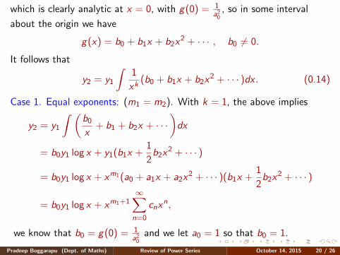
which is clearly analytic at x = 0, with g(0) = 1a20

, so in some interval

about the origin we have

g(x) = b0 + b1x + b2x2 + · · · , b0 6= 0.

It follows that

y2 = y1

∫1

xk(b0 + b1x + b2x

2 + · · · )dx . (0.14)

Case 1. Equal exponents: (m1 = m2). With k = 1, the above implies

y2 = y1

∫ (b0x

+ b1 + b2x + · · ·)dx

= b0y1 log x + y1(b1x +1

2b2x

2 + · · · )

= b0y1 log x + xm1(a0 + a1x + a2x2 + · · · )(b1x +

1

2b2x

2 + · · · )

= b0y1 log x + xm1+1∞∑n=0

cnxn,

we know that b0 = g(0) = 1a20

and we let a0 = 1 so that b0 = 1.


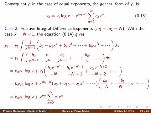
Consequently, in the case of equal exponents, the general form of y2 is

y2 = y1 log x + xm1+1∞∑n=0

cnxn. (0.15)

Case 2: Positive Integral Difference Exponents (m1 −m2 = N). With thecase k = N + 1, the equation (0.14) gives

y2 = y1

∫1

xN+1

(b0 + b1x

1 + b2x2 + · · ·+ bNx

N + · · ·)dx

= y1

∫ (b0

xN+1+

b1xN

+b2

xN−1+ · · ·+ bN

x+ · · ·

)dx

= bNy1 log x + y1

(b0x−N

−N+

b1x−N+1

−N + 1+

b2x−N+2

−N + 2+ · · ·

)= bNy1 log x + xm1−N(a0 + a1x + a2x

2 + · · · )(

b0−N

+b1

−N + 1x1 + · · ·

)= bNy1 log x + xm2

∞∑n=0

cnxn,


so that, the general form of second independent solution y2 is given by

y2 = bNy1 log x + xm2

∞∑n=0

cnxn, (0.16)

where c0 = −a0b0/N 6= 0. This gives the general form of y2 in the case ofexponents differing by a positive integer.

Note the coefficient bN that appear in the above equation but not in(0.15). If it happens that bN = 0, there there is no logarithmic term; if so,our differential equation has a second Frobenius series solution (Case C).


Summary: If the differential equation y ′′ + P(x)y ′ + Q(x)y = 0 has aregular point at x = 0 and the roots of indicial equation (m1, m2) arediffer by a fraction not by an integer then by Theorem A, the differentialequation has two independent Frobenius series solutions.

Otherwise, there two cases. In the case where m1 = m2, the equation hasonly one Frobenius series solution and has a second independet solution ofthe form (0.15) whcih contains logarithmic term.

In the case where m1 −m2 = N is a positive integer, the equationdefinitely has one Frobenius series solution and the second independentsolution will be of the form (0.16) in general which means that the secondindependent Frobenius series solution may or may not exist accordinglybN = 0 or bN 6= 0 in (0.16).

Exercise: Solve Problem no. 2, 3, 4, 5 and 6 in Section 30 in the textbook. Note that the some of these problems are solved in the classroom.




Thank you for your attention


Documents

Regular Singular Points - Frobenius Series Solutions ...universe.bits-pilani.ac.in/uploads/FSS.pdf · Regular Singular Points - Frobenius Series Solutions (Continued) Pradeep Boggarapu