Embed Size (px)
Citation preview
HAL Id: hal-01338023https://hal.archives-ouvertes.fr/hal-01338023
Preprint submitted on 27 Jun 2016
HAL is a multi-disciplinary open accessarchive for the deposit and dissemination of sci-entific research documents, whether they are pub-lished or not. The documents may come fromteaching and research institutions in France orabroad, or from public or private research centers.
L’archive ouverte pluridisciplinaire HAL, estdestinée au dépôt et à la diffusion de documentsscientifiques de niveau recherche, publiés ou non,émanant des établissements d’enseignement et derecherche français ou étrangers, des laboratoirespublics ou privés.
REGULAR VARIATION OF A RANDOM LENGTHSEQUENCE OF RANDOM VARIABLES AND
APPLICATION TO RISK ASSESSMENTC Tillier, O Wintenberger
To cite this version:C Tillier, O Wintenberger. REGULAR VARIATION OF A RANDOM LENGTH SEQUENCE OFRANDOM VARIABLES AND APPLICATION TO RISK ASSESSMENT. 2016. hal-01338023
REGULAR VARIATION OF A RANDOM LENGTH SEQUENCE OF RANDOM
VARIABLES AND APPLICATION TO RISK ASSESSMENT
C. TILLIER AND O. WINTENBERGER
Abstract. When assessing risks on a finite-time horizon, the problem can often be reduced to thestudy of a random sequence C(N) = (C1, . . . , CN ) of random length N , where C(N) comes from theproduct of a matrix A(N) of random size N ×N and a random sequence X(N) of random length N .Our aim is to build a regular variation framework for such random sequences of random length, tostudy their spectral properties and, subsequently, to develop risk measures. In several applications,many risk indicators can be expressed from the asymptotic behavior of ||C(N)||, for some norm‖ · ‖. We propose a generalization of Breiman Lemma that gives way to an asymptotic equivalent to‖C(N)‖ and provides risk indicators such as the ruin probability and the tail index for Shot NoiseProcesses on a finite-time horizon. Lastly, we apply our final result to a model used in dietary riskassessment and in non-life insurance mathematics to illustrate the applicability of our method.
1. Introduction
Risk analyses play a leading role within fields such as dietary risk, hydrology, nuclear security,finance and insurance. Moreover, risk analysis is present in the applications of various probabilitytools and statistical methods. We see a significant impact on the scientific literature and on publicinstitutions (see [7], [1], [12] or [16]).
In insurance, risk theory is useful for getting information regarding the amount of aggregate claimsthat an insurance company is faced with. By doing so, one may implement solvency measures toavoid bankruptcy; see [22] for a survey of non-life insurance mathematics. To further illustrate theimportance of risk analysis, we turn to the field of dietary risk. Here, toxicologists determine con-tamination levels which could later be used by mathematicians to build risk indicators. For example,in [6], authors proposed a dynamic dietary risk model, which takes into account both the eliminationand the accumulation of a contaminant in the human body; see [13], [14], and [7] for a survey ondietary risk assessment.
Besides, risk theory typically deals with the occurrences of rare events which are functions of heavy-tailed random variables, for example, sums or products of regularly varying random variables; see [18]and [21] for an exhaustive survey on regular variation theory. Non-life insurance mathematics anddietary risk management both deal with a particular kind of Shot Noise Processes S(t)t>0, definedas
(1) S(t) =
N(t)∑
n=0
Xih(t, Ti), t > 0,
where (Xi)i≥0 are independent and identically random variables, h is a measurable function andN(t)t>0 is a renewal process; see Section 4 for details. In this context, a famous risk indicatoris the ruin probability on a finite-time horizon that is the probability that the supremum of theprocess S exceeds a threshold on a time window [0, T ], for a given T > 0. It is straightforward thatmaxima necessarily occur on the embedded chain and it is enough to study the discrete-time randomsequence S(N(T )) := (S(T1), S(T2), . . . , S(TN(T ))), which is of random length N(T ). Then, instead of
Key words and phrases. Ruin theory, multivariate regular variation, risk indicators, Breiman Lemma, asymptoticproperties, stochastic processes, extremes, rare events.
1
2 CHARLES TILLIER AND OLIVIER WINTENBERGER
dealing with the extremal behavior of S(t)t≤T , we only need to understand the extremal behavior
of ‖S(N(T ))‖∞.We go further and point out that many risk measures in non-life insurance mathematics and in
dietary risk assessment can be analyzed from the tail behavior of ‖C(N)‖ where C(N) = (C1, . . . , CN )is a random sequence of random length N and ‖ · ‖ is a norm such that
(2) ‖ · ‖∞ ≤ ‖ · ‖ ≤ ‖ · ‖1.
Thus we consider discrete-time processes C(N) = (C1, . . . , CN ) where for all 1 ≤ i ≤ N , Ci ∈ R+
and N is an integer-valued random variable (r.v.), independent of the Ci’s. We are interesting in thecase when the Ci’s are regularly varying random variables. We restrict ourselves to the process C(N)which can be written in the form
(3) C(N) = A(N)X(N),
where X(N) = (X1, . . . , XN )′ is a random vector with identically distributed marginals which arenot necessarily independent and A(N) is a random matrix of random size N ×N independent of theentries Xi of the vector X(N) and of N . However, X(N) and A(N) are still dependent through Nthat determines their dimensions. Notice that C(N) covers a wide family of processes with possiblydependent (Xi)i≥0.
Our main objectives are: to define regular variation properties for a random length sequence ofrandom variables and to study the spectral properties in order to develop risk measures. As it willbecome clear later, the randomness of the size N of the vector C(N) makes it difficult to use thecommon definition of multivariate regular variation in terms of vague convergence; see [17]. Indeed, tohandle regular variation of a random sequence of random length, we need to define a regular variationframework for an infinite-dimensional space of sequences defined on (R+)N
∗
. We tackle the problemusing the notion of M-convergence, introduced recently in [20]. A main difference with the finite-dimensional case is that the choice of the norm matters as it determines the infinite-dimensional spaceto consider; see [5], [3], [25] and [26] for a comprehensive review of finite-dimensional multivariateregular variation theory.
The key point of our approach is the use of a norm satisfying (2) that allows to build regularvariation via polar coordinates. This approach combined with an extension of Breiman Lemma leadsto characterize the regular variation properties of C(N); see [10] for the statement and the proof ofBreiman Lemma. According to the choice of the norm, it characterizes several risk indicators for alarge family of processes.
For a particular class of Shot Noise Processes, we recover the result of [19] regarding the tail behaviorwhen N is a Poisson process and when the (Xi)i≥0 are asymptically independent and identicallydistributed. We give also the ruin probability for shot noise processes defined as (1) when the (Xi)i≥0
are not necessarily independent. Moreover, we shall supplement the information missing by these twoindicators by suggesting new ones; see Section 4 for details. We first turn our interest to the ExpectedSeverity, a widely-used risk indicator in insurance. It is an alternative to Value-at-Risk that is moresensitive to the losses in the tail of the distribution. Then, we shall introduce an indicator calledIntegrated Expected Severity which supplies information on the total losses themselves. Lastly, ourfocus will shift to the Expected Time Over a Threshold, which corresponds to the average time spentby the process above a given threshold.
The paper is constructed as follows: firstly, we specify the framework and describe the assumptionson the model. In Section 3, we define regular variation for a random length sequence of randomvariables, followed by an extension of Breiman Lemma. Next, we attempt to apply and develop riskindicators for a particular class of stochastic processes: the Shot Noise Processes. We also applyour final result to a model used in dietary risk assessment called Kinetic Dietary Exposure Modelintroduced in [6]. Finally, Section 5 is devoted to proving the main results of this paper.
REGULAR VARIATION OF A RANDOM LENGTH SEQUENCE OF RANDOM VARIABLES AND APPLICATION TO RISK ASSESSMENT3
2. Framework and assumptions
2.1. Regular variation in c‖·‖. In order to provide an extension of Breiman Lemma for the normof a sequence C(N) = (C1, . . . , CN ) defined as in (3), we define regular variation for any vectorX(N) = (X1, X2, . . . , XN , 0, . . .) when N is a strictly positive random integer. We denote by c00 theset of sequences with a finite number of non-zero components. To build a regular variation frameworkon this space seems to be very natural for our purpose but we cannot do it since c00 is not complete.Indeed, it is not closed in (l∞, ‖ · ‖∞). For example, consider the sequence of c00 with elementsui = (1, 1/2, 1/3, . . . , 1/i, 0, 0, . . .), i ∈ N. Its limit as i → ∞ is not an element of c00. Therefore, wewill choose the completion of c00 in l∞ space denoted by c‖·‖. In the rest of the paper, we write ‖ · ‖when the norm satisfies (2).
Definition 1. The space c‖·‖ is the completion of c00 in (R+)N equipped with the convergence in thesequential norm ‖ · ‖.
For example, c‖·‖∞= c0, the space of sequences whose limit is 0:
c0 :=
u = (u1, u2, . . .) ∈ (R+)N : limi→+∞
ui = 0
.
Furthermore, c‖·‖1= ℓ1(R+), the space of sequences such that
∑
i≥0 ui < ∞. In the following, weequip c‖·‖ with the canonical distance d generated by the norm such that for any sequence X,Y ∈ c‖·‖,d(X,Y ) = ‖X − Y ‖ and we denote by 0 = (0, 0, . . .) the null element in c‖·‖. Besides, for all j ≥ 1,we denote ej = (0, . . . , 0, 1, 0, . . .) ∈ c‖·‖ the canonical basis of c‖·‖ and we denote by S(∞), the unitsphere over c‖·‖ defined as S(∞) = X ∈ c‖·‖ : ‖X‖ = 1. As c‖·‖ is a Banach space, the notion ofweak convergence holds on c‖·‖ and one can also define regular variation as in [17].
Definition 2. A sequence X = (X1, X2, . . .) ∈ c‖·‖ is regularly varying if there exists a non-degeneratemeasure µ such that
µx(·) =P(x−1X ∈ ·)
P(‖X‖ > x)
ν−→x→∞
µ(·),
whereν
−→ refers to the vague convergence on the Borel σ−field of c‖·‖\0.
Here we want to avoid the approach using the vague convergence because it implies to find compactsets which may be complicated in several cases, especially in our infinite-dimensional framework. Weuse instead the ”M-convergence” as introduced by [20], which instead of working with compact setsdeals with special ”regions” that are bounded away (BA) from the cone C we choose to remove. TheseBA sets will replace the ”relatively compact sets” generating vague convergence.
We use the same notation as in [20], consider the unit sphere S(∞) over c‖·‖ and we take S = c‖·‖.We choose to remove C = 0 which is a closed space in c‖·‖ and in particular a cone. ThenSC = S\C = c‖·‖\ 0 is an open set and still a cone. Similarly, we take S′ = [0,∞]× S(∞) and weremoveC′ = 0×S(∞) which is closed in [0,∞]×S(∞) too. Moreover, for anyX ∈ c‖·‖, we choose thestandard scaling function g : (λ,X) −→ λX := (λX1, λX2, . . .), λ > 0, which is well suited for polarcoordinate transformations. For S′, we choose the scaling function (λ, (r,W )) −→ (λr,W ) in order tomake 0×S(∞) a cone. Let h be the polar transformation such that h : c‖·‖\ 0 −→ [0,∞]×S(∞)and for all X ∈ c‖·‖\0,
h : X −→ (||X ||, ||X ||−1X).
As c‖·‖ is a separable Banach space, we can apply [20] to define regular variation on this space fromthe M-convergence. Precisely, condition (4.2) is satisfied and Corollary 4.4 in [20] holds. Combiningwith Theorem 3.1 in [20] which ensures the homogeneity property of the limit measure µ such thatµ(λA) = λ−αµ(A), for some α > 0, λ > 0 and A ∈ c‖·‖\0, it leads to the following characterizationof regular variation in c‖·‖.
4 CHARLES TILLIER AND OLIVIER WINTENBERGER
Proposition 3. A sequence of random elements X = (X1, X2, . . .) ∈ c‖·‖\0 is regularly varying iff‖X‖ is regularly varying and
L(
‖X‖−1X | ‖X‖ > x)
−→x→∞
L(Θ),
for some random element Θ ∈ S(∞) and L(Θ) = P(Θ ∈ ·) is the spectral measure of X.
It means that the regular variation of X is completely characterized by the tail index α of ‖X‖ andthe spectral measure of X .
2.2. Assumptions. In order to get the spectral measure of any random sequence C(N) of randomlength N defined as in (3), we require the following conditions:
(H0) Length: N is a positive integer-valued r.v. such that E[N ] > 0 and admits moments of order2 + α+ ǫ, ǫ > 0.
(H0’) Poisson counting process: N is an inhomogeneous Poisson Process with intensity functionλ(·) and cumulative intensity function m(·).
(H1) Regular variation: The (Xi)i≥0 are identically distributed (i.d.) with common mean γ and
cumulative distribution function (c.d.f.) FX , such that the survival function FX = 1− FX isregularly varying with index α > 0, denoted by X ∈ RV−α.
(H2) Uniform asymptotic independence: We assume a uniform bivariate upper tail indepen-dence condition: for all i, j ≥ 1,
supi6=j
∣
∣
∣
∣
P(Xi > x,Xj > x)
P(X1 > x)
∣
∣
∣
∣
−→x→∞
0.
(H3) Regularity of the norm: The norm ‖ · ‖ satisfies ‖ · ‖∞ ≤ ‖ · ‖ ≤ ‖ · ‖1.(H4) Tail condition on the matrix A(N): The random entries (ai,j) of A(N) are independent
of the (Xi). Moreover, there exists some ǫ > 0 such that
E[||A(N)||α+ǫN1+α+ǫ] <∞,
where ‖ · ‖ also denotes the corresponding induced norm on the space of N -by-N matrices.(H5) The matrix A(N) is not null.
Let us discuss the assumptions. The condition (H1) implies that the regular variation of thesequence C(N) = (C1, . . . , CN ) defined as in (3) comes from the regular variation of the sequenceX(N) and (H2) means in addition that the probability of two components of the sequence X(N)exceeding a high threshold goes to 0. Combining (H1) and (H2), it appears that the regular variationof the sequence C(N) is mostly due to the regular variation of one of the component of X(N). Notethat if the Xi’s are exchangeable and asymptotically independent, then (H2) holds. An example ofa time series satisfying (H2) is a stochastic volatility model defined by
Xt = σtǫt, t ∈ Z,
where the innovations ǫt are standardized positive i.i.d. r.v.’s such that P(ǫ0 6= 0) > 0 and E(ǫ1+δt )
holds for some δ > 0. The volatility σt satisfies the equation
log(σt) = φ log(σt−1) + ξt, t ∈ Z,
with φ ∈ (0, 1), the innovations (ξt)t∈Z are i.i.d. r.v.’s independent of (ǫt)t∈Z such that E(ξ20) <∞ and P(ξt > x) ∼ Kx−αe−x when x → ∞ for some positive constants K and α 6= 1. Thisis a particular case of stochastic volatility models with Gamma-Type Log-Volatility when the log-volatility is a AR(1) model. One can check that σt and Xt are regularly varying with index α = 1.Moreover, (log(σ0), log(σh)) is asymptotically independent as well as (σ0, σh) and (X0, Xh) for anystrictly positive h; see [11] for details.
Besides, (H3) implies ℓ1(R+) ⊆ c‖·‖ ⊆ c0 and holds for any ℓp norm for 1 ≤ p ≤ ∞. This conditionis always assumed in the paper, even if many conditions could be weakened if we only considered thenorm ‖ · ‖∞. But our aim is to develop a method which can be applied for a broad class of processes
REGULAR VARIATION OF A RANDOM LENGTH SEQUENCE OF RANDOM VARIABLES AND APPLICATION TO RISK ASSESSMENT5
and norms. Finally, (H4) requires more finite moments on N than (H0). This condition can beviewed as an extension of the moment condition of the Breiman’s lemma. It is required to estimatethe tail of ‖C(N)‖ = ‖A(N)X(N)‖ from the one of ‖X(N)‖ and it is not restrictive in practice whenN satisfies (H0’).
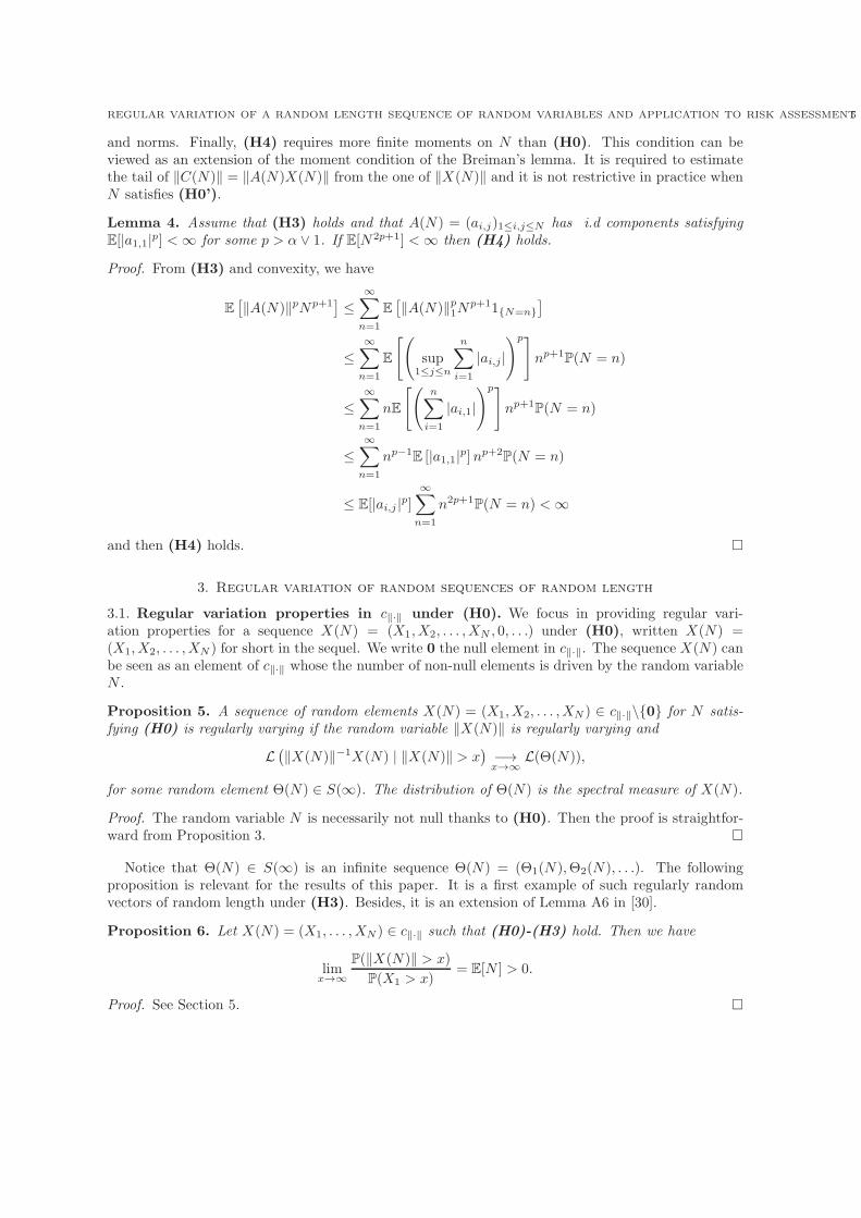
Lemma 4. Assume that (H3) holds and that A(N) = (ai,j)1≤i,j≤N has i.d components satisfyingE[|a1,1|
p] <∞ for some p > α ∨ 1. If E[N2p+1] <∞ then (H4) holds.
Proof. From (H3) and convexity, we have
E[
‖A(N)‖pNp+1]
≤
∞∑
n=1
E[
‖A(N)‖p1Np+11N=n
]
≤
∞∑
n=1
E
[(
sup1≤j≤n
n∑
i=1
|ai,j |
)p]
np+1P(N = n)
≤
∞∑
n=1
nE
[(
n∑
i=1
|ai,1|
)p]
np+1P(N = n)
≤
∞∑
n=1
np−1E [|a1,1|
p]np+2P(N = n)
≤ E[|ai,j |p]
∞∑
n=1
n2p+1P(N = n) <∞
and then (H4) holds.
3. Regular variation of random sequences of random length
3.1. Regular variation properties in c‖·‖ under (H0). We focus in providing regular vari-ation properties for a sequence X(N) = (X1, X2, . . . , XN , 0, . . .) under (H0), written X(N) =(X1, X2, . . . , XN ) for short in the sequel. We write 0 the null element in c‖·‖. The sequence X(N) canbe seen as an element of c‖·‖ whose the number of non-null elements is driven by the random variableN .
Proposition 5. A sequence of random elements X(N) = (X1, X2, . . . , XN ) ∈ c‖·‖\0 for N satis-fying (H0) is regularly varying if the random variable ‖X(N)‖ is regularly varying and
L(
‖X(N)‖−1X(N) | ‖X(N)‖ > x)
−→x→∞
L(Θ(N)),
for some random element Θ(N) ∈ S(∞). The distribution of Θ(N) is the spectral measure of X(N).
Proof. The random variable N is necessarily not null thanks to (H0). Then the proof is straightfor-ward from Proposition 3.
Notice that Θ(N) ∈ S(∞) is an infinite sequence Θ(N) = (Θ1(N),Θ2(N), . . .). The followingproposition is relevant for the results of this paper. It is a first example of such regularly randomvectors of random length under (H3). Besides, it is an extension of Lemma A6 in [30].
Proposition 6. Let X(N) = (X1, . . . , XN ) ∈ c‖·‖ such that (H0)-(H3) hold. Then we have
limx→∞
P(‖X(N)‖ > x)
P(X1 > x)= E[N ] > 0.
Proof. See Section 5.
6 CHARLES TILLIER AND OLIVIER WINTENBERGER
Here the moment condition in (H0) is required to handle the ‖ · ‖1 case. Releasing the assumption(H0), it is easy to draw an i.i.d. sequence of random length which is regularly varying in c‖·‖∞
butnot in c‖·‖1
. For instance, for the ‖ · ‖∞ case, the result is true under the integrability of N only butthis assumption is not sufficient to ensure the convergence for the ‖ · ‖1 case. Note also that (H3) isrequired since the convergence might not hold for some norms that do not satisfy (H3). From thisproposition, a characterization of the spectral measure of X(N) is possible.
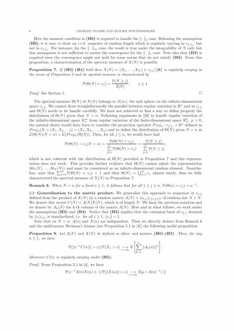
Proposition 7. If (H0)-(H3) hold then X(N) = (X1, . . . , XN ) ∈ c‖·‖\0 is regularly varying inthe sense of Proposition 5 and its spectral measure is characterized by
P(Θ(N) = ej) =P(N ≥ j)
E[N ], j ≥ 1.
Proof. See Section 5.
The spectral measure Θ(N) of X(N) belongs to S(∞), the unit sphere on the infinite-dimensionalspace c‖·‖. We cannot draw straightforwardly the parallel between regular variation in Rn and in c‖·‖and Θ(N) needs to be handle carefully. We have not achieved to find a way to define properly thedistribution of Θ(N) given that N = n. Following arguments in [20] to handle regular variation ofthe infinite-dimensional space R∞
+ from regular variation of the finite-dimensional space Rp+, p > 0,
the natural choice would have been to consider the projection operator Projn : c‖·‖ → Rn defined asProjn(X = (X1, X2, . . .)) = (X1, X2, . . . , Xn) and to define the distribution of Θ(N) given N = n asL(Θ(N)|N = n) = L(Projn(Θ(N)). Then, for all j ≤ n, we would have had
P(Θ(N) = ej |N = n) =P(Θ(N) = ej)n∑
j=1
P(Θ(N) = ej)=
P(N ≥ j)n∑
j=1
P(N ≥ j),
which is not coherent with the distribution of Θ(N) provided in Proposition 7 and this represen-tation does not work. This provides further evidence that Θ(N) cannot admit the representation(Θ1(N), . . . ,ΘN(N)) and must be considered as an infinite-dimensional random element. Nonethe-less, note that
∑∞j=1 P(Θ(N) = ej) = 1 and then Θ(N) =
⋃∞j=1 ej almost surely, thus we fully
characterized the spectral measure of X(N) in Proposition 7.
Remark 8. When N = n for a fixed n ≥ 1, it follows that for all 1 ≤ j ≤ n, P(Θ(n) = ej) = n−1.
3.2. Generalization to the matrix product. We generalize this approach to sequences in c‖·‖defined from the product of X(N) by a random matrix A(N) = (ai,j)1≤i,j≤N of random size N ×N .We denote this vector C(N) = A(N)X(N), which is of length N . We keep the previous notation andwe denote by Ak(N) the k-th column of the matrix A(N). Here and in what follows, we work underthe assumptions (H3) and (H4). Notice that (H3) implies that the canonical basis of c‖·‖ denotedby (ei)i≥1 is standardized, i.e. for all i ≥ 1, ‖ei‖ = 1.
Note that on N = n, A(n) and X(n) are independent. Then we directly deduce from Remark 8and the multivariate Breiman’s lemma (see Proposition 5.1 in [4]) the following useful proposition.
Proposition 9. Let A(N) and X(N) be defined as above and assume (H0)-(H3). Then, for anyn ≥ 1, we have
P(‖x−1C(n)‖ > x)/P(X1 > x) −→x→∞
E
[
n∑
k=1
‖Ak(n)‖α
]
.
Moreover C(n) is regularly varying under (H5).
Proof. From Proposition 5.1 in [4], we have
P(x−1A(n)X(n) ∈ ·)/P(‖X(n)‖ > x) −→x→∞
E[µ A(n)−1(·)]
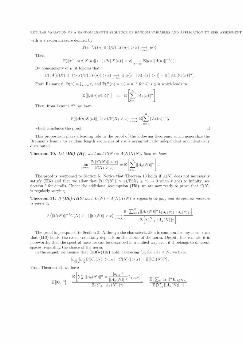
REGULAR VARIATION OF A RANDOM LENGTH SEQUENCE OF RANDOM VARIABLES AND APPLICATION TO RISK ASSESSMENT7
with µ a radon measure defined by
P(x−1X(n) ∈ ·)/P(‖X(n)‖ > x) −→x→∞
µ(·).
Then,
P(‖x−1A(n)X(n)‖ ∈ ·)/P(‖X(n)‖ > x) −→x→∞
E[µ ‖A(n)‖−1(·)].
By homogeneity of µ, it follows that
P(‖A(n)X(n)‖) > x)/P(‖X(n)‖ > x) −→x→∞
E[µx : ‖A(n)x‖ > 1] = E[‖A(n)Θ(n)‖α].
From Remark 8, Θ(n) =⋃
i≤n ei and P(Θ(n) = ei) = n−1 for all i ≤ n which leads to
E [‖A(n)Θ(n)‖α] = n−1E
[
n∑
k=1
‖Ak(n)‖α
]
,
Then, from Lemma 27, we have
P(‖A(n)X(n)‖) > x)/P(X1 > x) −→x→∞
E[
n∑
k=1
‖Ak(n)‖α],
which concludes the proof.
This proposition plays a leading role in the proof of the following theorems, which generalize theBreiman’s lemma to random length sequences of r.v.’s asymptotically independent and identicallydistributed.
Theorem 10. Let (H0)-(H4) hold and C(N) = A(N)X(N), then we have
limx→∞
P(‖C(N)‖ > x)
P(X1 > x)= E
[
N∑
k=1
||Ak(N)||α
]
.
The proof is postponed to Section 5. Notice that Theorem 10 holds if A(N) does not necessarilysatisfy (H5) and then we allow that P(‖C(N)‖ > x)/P(X1 ≥ x) → 0 when x goes to infinity; seeSection 5 for details. Under the additional assumption (H5), we are now ready to prove that C(N)is regularly varying.
Theorem 11. If (H0)-(H5) hold, C(N) = A(N)X(N) is regularly varying and its spectral measureis given by
P(
‖C(N)‖−1C(N) ∈ · | ‖C(N)‖ > x)
−→x→∞
E
[
∑Nk=1 ‖Ak(N)‖α11‖Ak(N)‖−1Ak(N)∈·
]
E
[
∑Nk=1 ‖Ak(N)‖α
]
The proof is postponed to Section 5. Although the characterization is common for any norm suchthat (H3) holds, the result essentially depends on the choice of the norm. Despite this remark, it isnoteworthy that the spectral measure can be described in a unified way even if it belongs to differentspaces, regarding the choice of the norm.
In the sequel, we assume that (H0)-(H5) hold. Following [5], for all i ≤ N , we have
limǫ→0
limx→∞
P(|Ci(N)| > xǫ | ||C(N)|| > x) = E [|Θi(N)|α] .
From Theorem 11, we have
E [|Θi|α] =
E
[
∑
k ||Ak(N)||α ×|ai,k|
α
||Ak(N)||α11i≤N
]
E [∑
k ||Ak(N)||α]=
E[∑
k |ak,i|α11i≤N
]
E [∑
k ||Ak(N)||α].
8 CHARLES TILLIER AND OLIVIER WINTENBERGER
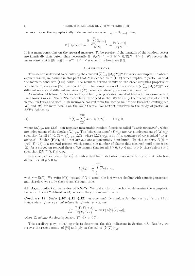
Let us consider the asymptotically independent case when ak,i = 11i=k then,
E [|Θi(N)|α] =
E
[
N∑
k=1
11i=k
]
E[N ]=
P(N ≥ i)
E(N).
It is a mean constraint on the spectral measure. To be precise, if the margins of the random vectorare identically distributed, then necessarily E [|Θi(N)|α] = P(N ≥ i)/E(N), i ≥ 1. We recover themean constraint E [|Θi(n)|
α] = n−1, 1 ≤ i ≤ n when n is fixed; see [15].
4. Applications
This section is devoted to calculating the constant∑N
k=1 ||Ak(N)||α for various examples. To obtainexplicit results, we assume in this part that N is defined as in (H0’) which implies in particular thatthe moment condition (H4) holds. The result is derived thanks to the order statistics property of
a Poisson process (see [22], Section 2.1.6). The computation of the constant∑N
k=1 ||Ak(N)||α fordifferent norms and different matrices A(N) permits to develop various risk measures.
As mentioned before, C(N) covers a wide family of processes. We deal here with an example of aShot Noise Process (SNP). SNP were first introduced in the 20’s to study the fluctuations of currentin vacuum tubes and used in an insurance context from the second half of the twentieth century; see[30] and [28] for more details on the SNP theory. We restrict ourselves to the study of particularSNP’s defined by
(4) Y (t) =
N(t)∑
i=1
Xi × hi(t, Ti), ∀ t ≥ 0,
where (hi)i≥0 are i.i.d. non-negative measurable random functions called ”shock functions”, whichare independent of the shocks (Xi)i≥0. The ”shock instants” (Ti)i≥0 are r.v.’s independent of (Xi)i≥0
such that for all i ≥ 0, Ti =∑
0≤k≤i ∆Tk, where (∆Tk)k≥0 is an i.i.d. sequence of r.v.’s called ”inter-
arrivals”. Under (H0’), the inter-arrivals are exponentially distributed. In this context, N(t) =#i : Ti ≤ t is a renewal process which counts the number of claims that occurred until time t; see[22] for a survey on renewal theory. We assume that for all i ≥ 0, t > 0 and α > 0, there exists ǫ > 0such that E[hα+ǫ
i (t, Ti)] <∞.
In the sequel, we denote by F IX the integrated tail distribution associated to the r.v. X , which is
defined for all y > 0 by
F IX(y) =
1
γ
+∞∫
y
FX(x)dx,
with γ = E(X). We write N(t) instead of N to stress the fact we are dealing with counting processesand therefore we study the process through time.
4.1. Asymptotic tail behavior of SNP’s. We first apply our method to determine the asymptoticbehavior of a SNP defined as (4) as a corollary of our main result.
Corollary 12. Under (H0’)-(H1)-(H2), assume that the random functions hj(T, ·)’s are i.i.d.,independent of the Tj’s and integrable of order p > α, then
limx→∞
P(Y (T ) > x)
P(X1 > x)= m(T )E[hα0 (T, V0)],
where V0 admits the density λ(t)/m(T ), 0 ≤ t ≤ T .
This corollary plays a leading role to determine the risk indicators in Section 4.3. Besides, werecover the recent results of [30] and [19] on the tail of Y (T )T≥0.
REGULAR VARIATION OF A RANDOM LENGTH SEQUENCE OF RANDOM VARIABLES AND APPLICATION TO RISK ASSESSMENT9
Proof. Let T be a strictly positive constant and let C(N(T )) = A(N(T ))X(N(T )) be a sequence ofrandom length N(T ) with A(N(T )), the diagonal matrix such that for all 1 ≤ j ≤ N(T ), ajj =
hj(T,Tj). Then, one can write Y (T ) =∑N(T )
j=1 Xjhj(T, Tj) = ‖C(N(T ))‖1. Using similar arguments
than in the proof of Lemma 4, we check that (H4) holds and we apply Theorem 10 in order to obtain
limx→∞
P(Y (T ) > x)
P(X1 > x)= E
N(T )∑
k=1
‖Ak(N(T ))‖α1
.
Note that for all k ≤ N(T ), ||Ak(N(T ))||α1 = hαk (T,Tk). Let V(k) be the k-th order statistic associated
to the i.i.d. sequence (V0, V1, . . .) distributed as V0. From [22], Section 2.1.6, (Tk | N(T ))d= V(k) and
it follows that
E
N(T )∑
k=1
hαk (T,Tk)
= E
E
N(T )∑
k=1
hαk (T,Tk) | N(T )
= E
E
N(T )∑
k=1
hαk (T,V(k)) | N(T )
= E
E
N(T )∑
k=1
hαk (T,Vk) | N(T )
= E[N(T )]E[hα0 (T, V0)],
which is the desired result.
Notice that the asymptotic behavior of Y (T ) as T → ∞ relies on the one of the shock functionh0. One case corresponds to E[N(T )]E[hα0 (T, V0)] → C for some constant, then Y (∞) may be welldefined. Thus, the SNP may admit a stationary distribution Y (∞) =
∑
i≥1Xi × hi(T, Ti) that is
regularly varying similarly than X1. Another case corresponds to E[N(T )]E[hα0 (T, V0)] → ∞ and thenit is very likely that Y (∞) = ∞ a.s.. In the latter case, we have explosive shot noise processes.
4.2. Ruin probability. We are interesting in determining the finite-time ruin probability ψ of a SNPdefined as in (4), which is the probability that Y (t) exceeds some given threshold x ∈ R+ on a period[0, T ], i.e.
ψ(x, T ) = P
(
sup0≤t≤T
Y (t) > x)
, T > 0.
Corollary 13. Assume that the conditions of Corollary 12 hold. If hj(·, T ) is a non-increasingfunction for any T > 0, then,
limx→∞
ψ(x, T )
P(X1 > x)= m(T )E[hα0 (V0, V0)].
Notice that if hj(·, T ) is a non-decreasing function for any T > 0, then the maximum of the SNPis achieved at time T and so the ruin probability can be computed thanks to Corollary 12. Anintermediate example is when the random shot function h0 can be either increasing and decreasing;see Section 4.4.
Proof of Corollary 13. Let T be a strictly positive constant. Note that in this setup, the maximum ofthe process Y (T )T≥0 is necessarily reached on its embedded chain Y (Ti)i≥0. Then, it is equivalent
to the study the tail of max1≤k≤N(T )
∑kj=1Xjhj(Tk, Tj). To do so, let C(N(T )) = A(N(T ))X(N(T ))
with A(N(T )), the lower triangular matrix such that ak,j = hj(Tk, Tj) for 1 ≤ j ≤ k and ak,j = 0 for
10 CHARLES TILLIER AND OLIVIER WINTENBERGER
k + 1 ≤ j ≤ N . Now, observe that max1≤k≤N(T )
∑kj=1Xjhj(Tk, Tj) = ‖C(N(T ))‖∞. We check that
(H4) holds thanks to Lemma 4 and from Theorem 10, we have
limx→∞
‖C(N(T ))‖∞P(X1 > x)
= E
N(T )∑
k=1
||Ak(N(T ))||α∞
.
Conditionally on N(T ), we have Aj(N(T )) = (0, . . . , 0, hj(V(j), V(j))), . . . , hj(V(N(T )), V(j)))′. Then,
‖Aj(N(T ))‖α∞ = hαj (V(j), V(j)) and with similar arguments than in the previous corollary, it followsthat
E
N(T )∑
k=1
||Ak(N)||α∞
= E [N(T )× E [hα0 (V0,V0)] ] ,
which concludes the proof.
Remark 14. If for T > 0, h0(T, T ) = c with c > 0, then Corollary 13 extends to any countingprocess N providing ψ(x, T ) ∼ cα E[N(T )]P(X1 > x) as x→ ∞. Besides, in such case where h0(T, T )is constant, a sandwich argument yields also the desired result. Indeed, we have
P
(
c maxi=1,...,N(T )
Xi > x
)
≤ P
(
maxi=1,...,N(T )
i∑
k=1
Xihi(T, Ti)
> x
)
≤ P
c
N(T )∑
i=1
Xi > x
.
So Proposition 6 can be directly used to find again that
ψ(x, T ) ∼x→∞
cαE[N(T )]P(X1 > x).
Remark 15. We obtain an asymptotic relation between the tail behavior and the ruin probability ofa process defined as in (4). Precisely, we have
P (Y (T ) > x) ∼x→∞
E [hα0 (T, V0)]
E[hα0 (V0, V0)]ψ(x, T )
when hj(·, T ) is a non-increasing function for any T and
P (Y (T ) > x) ∼x→∞
ψ(x, T )
when hj(·, T ) is an non-decreasing function.
4.3. Other risk indicators. We propose in this part three indicators to supplement the informationgiven by the ruin probability and the tail behavior. The ruin probability permits to know if theprocess has exceeded the threshold but provides no information about the exceedences themselves orabout the duration of the exceedences.
To fill the gap, we first bear our interest on the Expected Severity. Then, we present an indicatorcalled Integrated Expected Severity, which provides information on the total of the exceedences. Finally,we are interested in the Expected Time Over a Threshold which corresponds to the average time spentby the process over a threshold. We keep the previous notation and features on the process definedas (4).
4.3.1. The Expected Severity and the Integrated Expected Severity. Let us first begin with the ExpectedSeverity. By definition, the Expected Severity for a given threshold x, written ES(x), is the quantitydealing with the mean of the excesses knowing that the process has already reached the referencethreshold x, defined for all T > 0 by E[[Y (T )− x]+], where [·]+ is the positive part function.
Proposition 16. Assume that the conditions of Corollary 12 hold. For any T > 0, the expectedseverity of a process defined as (4) is given by
ES(x) ∼x→∞
γm(T )E[hα0 (T, V0)]FIX(x).
REGULAR VARIATION OF A RANDOM LENGTH SEQUENCE OF RANDOM VARIABLES AND APPLICATION TO RISK ASSESSMENT11
Proof. By definition,
E[Y (T )− x]+ = E
N(T )∑
i=1
Xihi(T, Ti)− x
+
=
+∞∫
x
P
N(T )∑
i=1
Xihi(T, Ti) > y
dy.
From Corollary 12, it follows that
ES(x) ∼x→∞
+∞∫
x
E[N(T )]E[hα0 (T, V0)]P (X > y)dy
∼x→∞
γE[N(T )]F IX(x)E[hα0 (T, V0)]
and the desired result follows.
Now, we bear our interest on the Integrated Expected Severity, denoted by IES(x) for any x > 0,which deals with the average of the cumulated exceedences when the process is over the threshold xon a time window [0, T ].
Proposition 17. Assume that the conditions of Corollary 12 hold. The Integrated Expected Severityfor a process defined as (4) for large values of x is given by
IES(x) ∼x→∞
γ
T∫
0
E[N(t)]E [hα0 (t, V0)] dt FIX(x).
Proof. By definition,
IES(x) =
∫ T
0
E[Y (t)− x]+dt.
From the previous Proposition, we directly obtain the result.
4.3.2. The Expected Time Over a Threshold. The Expected Time Over a reference threshold x, writtenETOT(x), provides information about how long does the process stay, in average, above a thresholdx, knowing that it has already reached it. It is defined for all x > 0 by
ETOT (x) = E
T∫
0
11Y (t)∈]x,∞[dt | max0≤t≤T
Y (t) > x
.
Proposition 18. Assume that the conditions of Corollary 12 hold. For large values of x, the ETOT(x)for the process defined as (4) is given by
ETOT (x) ∼x→∞
T∫
0
m(t)E[hα0 (t, V0)]dt
m(T )E[hα0 (V0, V0)].
Proof. By definition,
ETOT (x) =
E
[
T∫
0
11Y (t)∈]x,∞[dt
]
ψ(x, T ).
Let A(N(t)) be the diagonal matrix such that for all 1 ≤ j ≤ N(t), ajj = hj(t, Tj). Note that
T∫
0
E[11Y (t)>x]dt =
T∫
0
P(Y (t) > x)dt =
T∫
0
P(‖C(N(t))‖1 > x)dt.
Plug-in Corollary 12 in the previous expression concludes the proof.
12 CHARLES TILLIER AND OLIVIER WINTENBERGER
Remark 19 (The extremal index for shot noise processes). Under the previous assumptions, we definethe extremal index θ ∈ [0,∞] as the inverse of lim
T→∞limx→∞
ETOT (x) if it exists, i.e.
T∫
0
m(t)E[hα0 (t, V0)]dt
m(T )E[hα0 (V0, V0)]−→T→∞
1
θ.
It can be seen as a continuous version of the extremal index for discrete time-series; see [27]. Tobe precise, it measures the clustering tendency of high threshold exceedences and how the extremevalues cluster together. In this context, θ does not still belong to [0, 1] but to [0,∞]. Notwithstanding,the inverse of the extremal index θ−1 indicates somehow, how long (in mean) an extremal event willoccur, due to the dependency structure of the data. For instance θ = 0 for a random walk such thathi = 1 and extremal events may long forever. At the opposite, in the asymptotic independent casehi(t, v) = 11t=v, then θ = +∞ and extremal events occur instantaneous only.
4.4. Application in dietary risk assessment and in non-life insurance mathematics. Theshot noise process defined as in (4) intervenes in many applications in which sudden jumps occur suchas in insurance to model the amount of aggregate claims that an insurer has to cope with; see [2] and[12] and [22].
In dietary risk assessment and non-life insurance, we typically consider deterministic shock functionsdefined for all 0 ≤ x ≤ t by h(t, x) = e−ω(t−x), with a shape parameter ω > 0; see [6], [7] and [22] formore details. We call this model Exp-SNP for Exponential Shot Noise Process.
In [6], authors suggested a model, called Kinetic Dietary Exposure Model (KDEM ), to representthe evolution of a contaminant in the human body. Their model is a discrete-time risk process whichcan be expressed from a Exp-SNP on the shock intants; see Remark 21. In this context, shocks areregularly varying distributed intakes which arise according to N(T ) and ω is an elimination parameter.
We consider below an extension of the KDEM process. The main novelty is as follows: we areinterested in the case when the ω = ωi ∈ Ω are i.i.d. r.v.’s and may take negative values satisfyingthe Cramer’s condition E[exp(pω−T )] < ∞ for some p > α and ω− = max(−ω, 0). Then, the modelis defined by
(5) Y (t) =
N(t)∑
i=1
Xie−ωi(t−Ti), ∀ t ≥ 0.
Here again, we can assume the the (Xi)i≥1 are asymptotically independent and identically regularlyvarying random variables. In dietary risk assessment, it makes sense to consider such random elimi-nation parameter to take into account interactions between different human organs. Thus, ω can beseen as a ”inhibitor factor”, for positive values of ω, or contrariwise, a ”catalytic factor” for negativevalues of ω. In insurance, these Exp-SNP are often used and the parameter ωi = ω can be seen as anaccumulation (resp. discount) factor when ω is a strictly negative (resp. positive) constant. Here themodel is such that usually a discount factor applies on the risk except in some cases when it is theopposite and there is accumulation of the risk.
Assuming an homogeneous Poisson process on the distribution of claims instants such that λ(s) = λfor all 0 < s ≤ t, we obtain explicit formula for all the risk measures. Precisely,
Corollary 20. Let Y (t) follow the KDEM defined in (5) with random elimination parameter ω such
that (H0’)-(H1)-(H2) hold. Then we have θ = αE[ω2]
E[ω]for ω > 0 a.s., θ = αω− if P(ω < 0) > 0
REGULAR VARIATION OF A RANDOM LENGTH SEQUENCE OF RANDOM VARIABLES AND APPLICATION TO RISK ASSESSMENT13
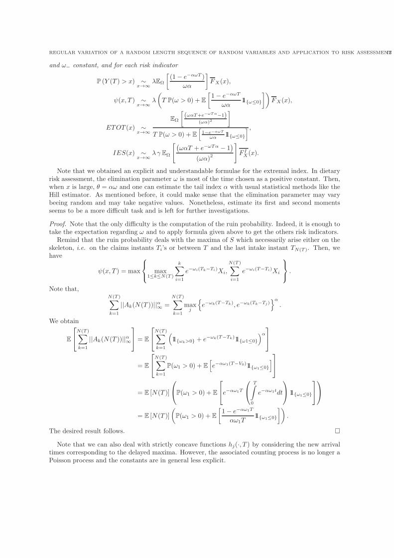
and ω− constant, and for each risk indicator
P (Y (T ) > x) ∼x→∞
λEΩ
[
(1− e−αωT )
ωα
]
FX(x),
ψ(x, T ) ∼x→∞
λ
(
T P(ω > 0) + E
[
1− e−αωT
ωα11ω≤0
])
FX(x),
ETOT (x) ∼x→∞
EΩ
[
(ωαT+e−ωTα−1)(ωα)2
]
T P(ω > 0) + E
[
1−e−αωT
ωα 11ω≤0
] ,
IES(x) ∼x→∞
λγ EΩ
[
(
ωαT + e−ωTα − 1)
(ωα)2
]
F IX(x).
Note that we obtained an explicit and understandable formulae for the extremal index. In dietaryrisk assessment, the elimination parameter ω is most of the time chosen as a positive constant. Then,when x is large, θ = αω and one can estimate the tail index α with usual statistical methods like theHill estimator. As mentioned before, it could make sense that the elimination parameter may varybeeing random and may take negative values. Nonetheless, estimate its first and second momentsseems to be a more difficult task and is left for further investigations.
Proof. Note that the only difficulty is the computation of the ruin probability. Indeed, it is enough totake the expectation regarding ω and to apply formula given above to get the others risk indicators.
Remind that the ruin probability deals with the maxima of S which necessarily arise either on theskeleton, i.e. on the claims instants Ti’s or between T and the last intake instant TN(T ). Then, wehave
ψ(x, T ) = max
max1≤k≤N(T )
k∑
i=1
e−ωi(Tk−Ti)Xi,
N(T )∑
i=1
e−ωi(T−Ti)Xi
.
Note that,N(T )∑
k=1
||Ak(N(T ))||α∞ =
N(T )∑
k=1
maxj
e−ωk(T−Tk), e−ωk(Tk−Tj)α
.
We obtain
E
N(T )∑
k=1
||Ak(N(T ))||α∞
= E
N(T )∑
k=1
(
11ωk>0 + e−ωk(T−Tk)11ω1≤0
)α
= E
N(T )∑
k=1
P(ω1 > 0) + E
[
e−αω1(T−V0)11ω1≤0
]
= E [N(T )]
P(ω1 > 0) + E
e−αω1T
T∫
0
e−αω1tdt
11ω1≤0
= E [N(T )]
(
P(ω1 > 0) + E
[
1− e−αω1T
αω1T11ω1≤0
])
.
The desired result follows.
Note that we can also deal with strictly concave functions hj(·, T ) by considering the new arrivaltimes corresponding to the delayed maxima. However, the associated counting process is no longer aPoisson process and the constants are in general less explicit.
14 CHARLES TILLIER AND OLIVIER WINTENBERGER
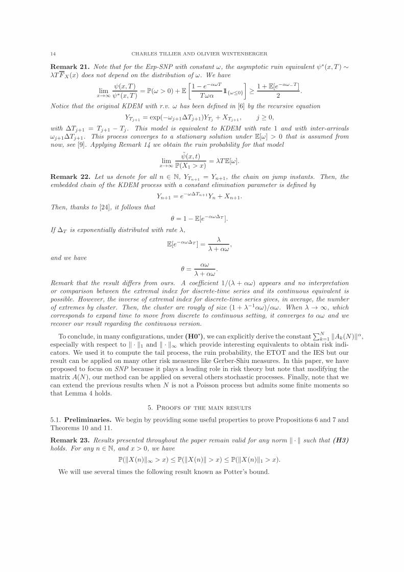
Remark 21. Note that for the Exp-SNP with constant ω, the asymptotic ruin equivalent ψ∗(x, T ) ∼λTFX(x) does not depend on the distribution of ω. We have
limx→∞
ψ(x, T )
ψ∗(x, T )= P(ω > 0) + E
[
1− e−αωT
Tωα11ω≤0
]
≥1 + E[e−αω−T ]
2.
Notice that the original KDEM with r.v. ω has been defined in [6] by the recursive equation
YTj+1= exp(−ωj+1∆Tj+1)YTj
+XTj+1, j ≥ 0,
with ∆Tj+1 = Tj+1 − Tj. This model is equivalent to KDEM with rate 1 and with inter-arrivalsωj+1∆Tj+1. This process converges to a stationary solution under E[ω] > 0 that is assumed fromnow, see [9]. Applying Remark 14 we obtain the ruin probability for that model
limx→∞
ψ(x, t)
P(X1 > x)= λTE[ω].
Remark 22. Let us denote for all n ∈ N, YTn+1= Yn+1, the chain on jump instants. Then, the
embedded chain of the KDEM process with a constant elimination parameter is defined by
Yn+1 = e−ω∆Tn+1Yn +Xn+1.
Then, thanks to [24], it follows that
θ = 1− E[e−αω∆T ].
If ∆T is exponentially distributed with rate λ,
E[e−αω∆T ] =λ
λ+ αω,
and we have
θ =αω
λ+ αω.
Remark that the result differs from ours. A coefficient 1/(λ + αω) appears and no interpretationor comparison between the extremal index for discrete-time series and its continuous equivalent ispossible. However, the inverse of extremal index for discrete-time series gives, in average, the numberof extremes by cluster. Then, the cluster are rougly of size (1 + λ−1αω)/αω. When λ → ∞, whichcorresponds to expand time to move from discrete to continuous setting, it converges to αω and werecover our result regarding the continuous version.
To conclude, in many configurations, under (H0’), we can explicitly derive the constant∑N
k=1 ‖Ak(N)‖α,especially with respect to ‖ · ‖1 and ‖ · ‖∞ which provide interesting equivalents to obtain risk indi-cators. We used it to compute the tail process, the ruin probability, the ETOT and the IES but ourresult can be applied on many other risk measures like Gerber-Shiu measures. In this paper, we haveproposed to focus on SNP because it plays a leading role in risk theory but note that modifying thematrix A(N), our method can be applied on several others stochastic processes. Finally, note that wecan extend the previous results when N is not a Poisson process but admits some finite moments sothat Lemma 4 holds.
5. Proofs of the main results
5.1. Preliminaries. We begin by providing some useful properties to prove Propositions 6 and 7 andTheorems 10 and 11.
Remark 23. Results presented throughout the paper remain valid for any norm ‖ · ‖ such that (H3)holds. For any n ∈ N, and x > 0, we have
P(‖X(n)‖∞ > x) ≤ P(‖X(n)‖ > x) ≤ P(‖X(n)‖1 > x).
We will use several times the following result known as Potter’s bound.
REGULAR VARIATION OF A RANDOM LENGTH SEQUENCE OF RANDOM VARIABLES AND APPLICATION TO RISK ASSESSMENT15
Proposition 24. Let F ∈ RV−α. Under (H0), there exists ǫ > 0 such that E[Nα+ǫ+1] < ∞ andthere exist x0 > 0, c > 1 such that for all y ≥ x ≥ x0, we have
c−1(y/x)−α−ǫ ≤F (y)
F (x)≤ c(y/x)−α+ǫ.
Proof. See [29].
Let us provide a technical lemma useful in the proofs:
Lemma 25. Let X(n) = (X1, X2, . . . , Xn) be a sequence such that (H1)-(H2) hold. Let f and g bestrictly positive functions such that for all n ∈ N∗, f(n) ≤ g(n) ≤ 1. Then, for any fixed n ≥ 1 andǫ > 0, there exists b(x) →
x→∞0 such that
n∑
i=1,i6=j
P (Xi > f(n)x ,Xj > g(n)x)
P (Xj > x)≤ f(n)−α+ǫn2b(x).
Proof. Let 1 ≤ i 6= j ≤ n, with j ≥ 1 and n ∈ N∗. Then, using Potter’s bound, for x sufficiently large
n∑
i=1,i6=j
P (Xi > f(n)x ,Xj > g(n)x)
P (Xj > x)≤
n∑
i=16=j
P (Xi > f(n)x ,Xj > f(n)x)
P (Xj > x)
≤
n∑
i=1,i6=j
P (Xi > f(n)x ,Xj > f(n)x) /P (Xj > f(n)x)
P (Xj > x) /P (Xj > f(n)x)
≤ c
n∑
i=1,i6=j
f(n)−α+ǫP (Xi > f(n)x ,Xj > f(n)x)
P (Xj > f(n)x)
≤ cf(n)−α+ǫn∑
i=1,i6=j
supi,j
P (Xi > f(n)x ,Xj > f(n)x)
P (Xj > f(n)x)
≤ cf(n)−α+ǫn(n− 1)
(
supi,j
P (Xi > f(n)x ,Xj > f(n)x)
P (Xj > f(n)x)
)
,
which combined with (H2) concludes the proof.
The following lemma plays a leading role in the sequel. It can be seen as an uniform integrabilitycondition which allows in the main body of Propositions 6 and 7 to integrate with respect to N ; see[8], Section 3.
Lemma 26. Let N be a random length satisfying (H0). Let X = (X1, X2, . . .) ∈ R∞+ be a sequence
such that (H1)-(H2) hold. Let A = (ai,j)i,j≥1 be the double indexed sequence of the coefficientssatisfying (H4) and define EA[·] (respectively PX [·]) the expectation (resp. the probability) with respectto A (resp. X). Then, for any fixed n0 ∈ N∗ and for any norm ‖ · ‖ such that (H3) holds, we havethe following statement:
limn0→∞
supx>0
(
EA
[
∞∑
n=n0+1
P(N = n)P(‖A(n)X(n)‖ > x)
P(X1 > x)
])
= 0.
Proof. Note first that
I(x) = supx>0
(
EA
[
∞∑
n=n0+1
P(N = n)P(‖A(n)‖‖X(n)‖ > x)
P(X1 > x)
])
≤ EA
[
supx>0
(
∞∑
n=n0+1
P(N = n)P((‖A(n)‖ ∨ 1)‖X(n)‖ > x)
P(X1 > x)
)]
16 CHARLES TILLIER AND OLIVIER WINTENBERGER
where (a∨ b) = max(a, b) for any a, b ∈ R+. For a fixed x0 > 0 defined as in Proposition 24, denotingy = x0(‖A(n)‖ ∨ 1), we have
I(x) ≤ EA
supx>0
(x/y∨n0)∑
n=n0+1
P(N = n)P((‖A(n)‖ ∨ 1)‖X(n)‖ > x)
P(X1 > x)
+ EA
supx>0
∞∑
n>(x/y∨n0)
P(N = n)P((‖A(n)‖ ∨ 1)‖X(n)‖ > x)
P(X1 > x)
≤ EA
[
supx>ny
(
∞∑
n=n0+1
P(N = n)P((‖A(n)‖ ∨ 1)‖X(n)‖ > x)
P(X1 > x)
)]
+ EA
supx>0
∞∑
n>(x/y∨n0)
P(N = n)P((‖A(n)‖ ∨ 1)‖X(n)‖ > x)
P(X1 > x)
≤ EA
[
supx>ny
(
∞∑
n=n0+1
P(N = n)P((‖A(n)‖ ∨ 1)‖X(n)‖ > x)
P(X1 > x)
)]
+ EA
[
supx>0
(
P(N > (x/y ∨ n0)
P(X1 > x)
)]
≤ I1(x) + I2(x).
Let us first investigate I1(x). For every fixed x > 0 and n > 0, we have
EA [P ((‖A(n)‖ ∨ 1)‖X(n)‖ > x)] ≤ EA [P (‖X(n)‖1 > x/(‖A(n)‖ ∨ 1))]
≤ EA
[
n∑
i=1
PX1(Xi > x/n(‖A(n)‖ ∨ 1))
]
= nEA [PX1(X1 > x/n(‖A(n)‖ ∨ 1))] .
Then,
I1(x) ≤ EA
[
supx>ny
(
∞∑
n=n0+1
nP(N = n)PX1
(X1 > x/n(‖A(n)‖ ∨ 1))
P(X1 > x)
)]
.
Using the Potter’s bound, there exists c > 1 independent of y ≥ 1 such that
supx≥ny
PX1(X1 > x/n(‖A(n)‖ ∨ 1))
P(X1 > x)≤ cnα+ǫ(‖A(n)‖α+ǫ ∨ 1).
It follows from (H4) that
I1(x) ≤ c∞∑
n=n0+1
P(N = n)nα+1+ǫE[
(‖A(N)‖α+ǫ ∨ 1)|N = n]
−→n0→∞
0.
We focus now on I2(x). From Markov inequality, for any x > 0 and for any ǫ > 0, under (H0), thereexists a constant c > 0 such that
EA[P(N > (x/y ∨ n0))] ≤ EA
[
E[Nα+ǫ]
(x/y ∨ n0)α+ǫ
]
≤ cEA
[
1
(x/y ∨ n0)α+ǫ
]
.
REGULAR VARIATION OF A RANDOM LENGTH SEQUENCE OF RANDOM VARIABLES AND APPLICATION TO RISK ASSESSMENT17
Moreover, we have
EA
[
supx≤n0y
P(N > (x/y ∨ n0))
P(X1 > x)
]
≤ c
(
EA
[
supx≤n0y
(x/y ∨ n0)−α−ǫ
P(X1 > x)
]
+ EA
[
supx≥n0y
(x/y ∨ n0)−α−ǫ
P(X1 > x)
])
≤ c
(
EA
[
n−α−ǫ0
P(X1 > n0y)
]
+ EA
[
supx≥n0y
(y/x)α+ǫ
P(X1 > x)
])
Notice that that from (H4) the moments of order α + ǫ of ‖A‖ are finite and so E[yα+ǫ] < ∞. Weuse again the Potter’s bound and, for a possibly different constant c > 0 (independent of y > 1) andn0 sufficiently large, we obtain
I2(x) ≤ cEA
[
yα+ǫ]
(
n−α−ǫ0
P(X1 > n0)+ sup
x≥n0
x−α−ǫ
P(X1 > x)
)
−→n0→∞
0.
We finally obtain
limn0→∞
I(x) = 0
which concludes the proof.
5.2. Proof of Proposition 6. We first state a lemma which can be seen as a generalization of awell-known property for i.i.d. regularly varying r.v.’s with respect to the infinite norm ‖ · ‖∞, whichmeans that the maximum of a sequence satisfying (H1) is reached just by one coordinate. Note thecrucial role of the uniform asymptotic independence condition (H2) in the sequel.
Lemma 27. Let X(n) = (X1, X2, . . . , Xn) be a sequence of r.v.’s such that (H1)-(H2) hold and ‖ · ‖satisfies (H3). Then,
limx→∞
P(||X(n)|| > x)
nP(X1 > x)= 1,
for any fixed n ≥ 1.
Proof. We proceed by upper and lower bounding the quantity
A(x) =P(||X(n)|| > x)− nP(X1 > x)
nP(X1 > x).
From Remark 23, under (H3), it is enough to investigate the lower (respectively the upper) boundwith respect to ‖ · ‖∞ (resp. ‖ · ‖1). For the lower bound, using the Bonferroni bound, for any fixedn ≥ 1 and x > 0, we have
P(‖X(n)‖∞ > x) = P
(
n⋃
i=1
Xi > x
)
≥ nP (Xi > x) −
n∑
i=1,i6=j
P(Xi > x,Xj > x).
Then, from Lemma 25 and Remark 23, it follows that
A(x) ≥ −
n∑
i=1,i6=j
P(Xi > x,Xj > x)
P(Xj > x)−→x→∞
0.
For the upper bound, let us consider ε such that 12 < ε < 1. Then, for all x > 0 and n ≥ 1,
P(‖X(n)‖1 > x) = P
(
n∑
i=1
Xi > x
)
≤ P
(
n⋃
i=1
Xi > εx
)
+ P
n∑
i=1
Xi > x,
n⋂
j=1
(Xj ≤ εx)
= A1(ε, x) +A2(ε, x).
18 CHARLES TILLIER AND OLIVIER WINTENBERGER
Using an union bound again and (H1), we obtain
lim supx→∞
A1(ε, x)n∑
i=1
P (Xi > x)≤ lim sup
x→∞
n∑
i=1
P (Xi > εx)
n∑
i=1
P (Xi > x)= ε−α.
Letting ε→ 1−, we obtain
lim supx→∞
A1(ε, x)n∑
i=1
P (Xi > x)≤ 1
which implies that
lim supx→∞
P (‖X(n)‖1 > x) −
n∑
i=1
P (Xi > x) ≤ lim supε→1−
lim supx→∞
A2(ε, x).
On the other hand, we have
A2(ε, x) = P
n∑
i=1
Xi > x,
n⋂
j=1
(Xj ≤ εx), max1≤k≤n
Xk >x
n
≤
n∑
k=1
P
(
n∑
i=1
Xi > x, Xk ≤ εx, Xk >x
n
)
≤n∑
k=1
P
n∑
i=1,i6=k
Xi > (1− ε)x, Xk >x
n
≤n∑
k=1
n∑
i=1,i6=k
P
(
Xi >(1− ε)x
n− 1, Xk >
x
n
)
.
Besides, applying Lemma 25 with f(n) =1− ε
n− 1and g(n) =
x
n, we obtain
lim supx→∞
A(x) ≤ lim supx→∞
A2(ε, x)n∑
i=1
P (Xi > x)≤ lim sup
x→∞
n∑
k=1
n∑
i=1,i6=k
P
(
Xi >(1−ε)xn−1 , Xk >
xn
)
n∑
i=1
P (Xi > x)
≤ lim supx→∞
n∑
k=1
n∑
i=1,i6=k
P
(
Xi >(1−ε)xn−1 , Xk >
xn
)
P (Xk > x)
= 0.
Collecting the bounds and using a sandwich argument leads to
limx→∞
A(x) = 0
for any fixed n ∈ N∗, which concludes the proof.
Proof of Proposition 6. From Lemma 27, for every fixed n0 > 0, we have
n0∑
n=1
P(N = n)P(‖X(n)‖ > x)
P(X1 > x)−→x→∞
n0∑
n=1
nP(N = n).
REGULAR VARIATION OF A RANDOM LENGTH SEQUENCE OF RANDOM VARIABLES AND APPLICATION TO RISK ASSESSMENT19
Besides, under (H0)-(H3), takingA(n) = In, with In the identity matrix of size n×n, the assumptionsof Lemma 26 hold. Then, from Remark 23,
limn0→∞
supx>0
∞∑
n=n0+1
P(N = n)P(‖X(n)‖ > x)
P(X1 > x)= 0,
for any norm ‖ · ‖ such that (H3) holds which insures the uniform integrability with respect to N .Letting n0 → ∞ in the first expression concludes the proof.
5.3. Proof of Proposition 7. Let X(n) = (X1, . . . , Xn) be a sequence such that (H1)-(H2) holdand let ‖ · ‖ satisfying (H3). We need the following characterization.
(6) L
(
X(n)
‖X(n)‖| ‖X(n)‖ > x
)
−→x→∞
L(Θ(n)),
with Θ(n) which does not depend on the choice of the norm ‖ · ‖. Specifically P(Θ(n) = ej) = n−1
which is consistent with Remark 8. We did not find a proper reference of this simple result andits proof follows: by asymptotical independence, the support of the spectral measure is concen-trated on the canonical basis ∪n
j=1ej and the measure is fully characterized by the probability
pj = P(Θ(n) = ej) = P(Yj(n) ≥ 1) where Yj(n) = Θj(n)Y (n), 1 ≤ j ≤ n. By definition of Θ(n), wealso have P(Yj(n) ≥ 1) = limx→∞ P(Xj(n) ≥ x | ‖X(n)‖ ≥ x) = n−1 from Lemma 27.
Now, let X(N) = (X1, . . . , XN ) be a a sequence such that (H0-(H2) hold. We first need to provethat for any norm || · || satisfying (H3),
limx→∞
P
(∣
∣
∣
∣
∣
∣
∣
∣
X(N)
||X(N)||−Θ(N)
∣
∣
∣
∣
∣
∣
∣
∣
> ǫ | ||X(N)|| > x
)
= 0.
From (6), the Skorohod’s representation theorem and Lemma 27, it follows that for any fixed n ∈ N∗,for any norm ‖ · ‖ such that (H3) holds and for any ǫ > 0, we have
limx→∞
P
(∣
∣
∣
∣
∣
∣
X(n)||X(n)|| −Θ(n)
∣
∣
∣
∣
∣
∣ > ǫ , ||X(n)|| > x)
nP(X1 > x)= 0.
Then,
limx→∞
P
(∣
∣
∣
∣
∣
∣
X(n)||X(n)|| −Θ(n)
∣
∣
∣
∣
∣
∣ > ǫ , ||X(n)|| > x)
P(X1 > x)= 0.
Moreover,
P
(∣
∣
∣
∣
∣
∣
X(n)||X(n)|| −Θ(n)
∣
∣
∣
∣
∣
∣ > ǫ , ||X(n)|| > x)
P(X1 > x)≤
P(‖X(n)‖ > x)
P(X1 > x),
and the uniform integrability criteria holds, which leads to
limx→∞
∞∑
n=1
P
(∣
∣
∣
∣
∣
∣
X(n)||X(n)|| −Θ(n)
∣
∣
∣
∣
∣
∣ > ǫ , ||X(n)|| > x)
P(X1 > x)P(N = n) = 0.
Finally, thanks to Proposition 6 we know that ‖X(N)‖ is regularly varying, and for any ǫ > 0 we have
P
(∣
∣
∣
∣
∣
∣
∣
∣
X(N)
||X(N)||−Θ(N)
∣
∣
∣
∣
∣
∣
∣
∣
> ǫ | ||X(N)|| > x
)
−→x→∞
0.
20 CHARLES TILLIER AND OLIVIER WINTENBERGER
We can now proceed to the characterization of the spectral measure. For allX(N) = (X1, X2, · · · , XN) ∈c‖·‖\0, we have
P(
‖X(N)‖−1X(N) ∈ · | ‖X(N)‖ > x)
=
∞∑
n=1P(
‖X(N)‖−1X(N) ∈ · , ‖X(N)‖ > x | N = n)
P(N = n)
∞∑
n=1P (‖X(N)‖ > x | N = n)P(N = n)
=
∞∑
n=1P(
‖X(n)‖−1X(n) ∈ · , ‖X(n)‖ > x)
P(N = n)
∞∑
n=1P (‖X(n)‖ > x)P(N = n)
=
∞∑
n=1P(
‖X(n)‖−1X(n) ∈ · , ‖X(n)‖ > x)
P(N = n) / P(X1 > x)
∞∑
n=1P (‖X(n)‖ > x)P(N = n) / P(X1 > x)
.
Then, from what preceeds and Lemma 27, we get for all j ≥ 1
P(
‖X(N)‖−1X(N) = ej | ‖X(N)‖ > x)
∼x→∞
∞∑
n=j
P(N = n)
∞∑
n=1nP(N = n)
∼x→∞
P(N ≥ j)
E[N ],
and the desired result follows.
5.4. Proof of Theorem 10. From Proposition 9, for any fixed n0, we have
n0∑
n=1
P(‖C(n)‖ > x)
P(X1 > x)P(N = n) −→
x→∞
n0∑
n=1
E
[
n∑
k=1
‖Ak(n)‖α]
P(N = n).
From Lemma 26, the uniform integrability of P(‖C(n)‖ > x)/P(X1 > x) with respect to N holds, onecan let n0 tends to +∞ above which concludes the proof.
5.5. Proof of Theorem 11. Let us use a similar but slightly but more evolved reasoning to proveTheorem 11. From Theorem 10, if we assume (H5), as the ai,j are not all identically null we have
(7) limx→∞
P(‖C(N)‖ > x)
P(X1 > x)= E
N∑
j=1
‖Aj(N)‖α
> 0,
and then ‖C(N)‖ is regularly varying. It remains to prove the existence of the spectral measure. FromProposition 6, we have
Px,n(·) = P(‖C(N)‖−1C(N) ∈ · | ‖C(N)‖ > x,N = n)
=P(‖C(N)‖−1C(N) ∈ ·, ‖C(N)‖ > x,N = n)
P(‖C(N)‖ > x,N = n)
=P(‖C(n)‖−1C(n) ∈ ·, ‖C(n)‖ > x)
P(X1 > x)
P(X1 > x)
P(‖C(n)‖ > x).
Consider n sufficiently large such that E[‖A(n)Θ(n)‖α] > 0. Applying the regular varying propertiesstated in Proposition 9, we have
limx→∞
P(X1 > x)
P(‖C(n)‖ > x)=
1
E[‖A(n)Θ(n)‖αn].
REGULAR VARIATION OF A RANDOM LENGTH SEQUENCE OF RANDOM VARIABLES AND APPLICATION TO RISK ASSESSMENT21
Then,
limx→∞
Px,n(·) = limx→∞
P(‖A(n)X(n)‖−1A(n)X(n) ∈ ·, ‖A(n)X(n)‖ > x)
E[‖A(n)Θ(n)‖αn]P(X1 > x)
and, as X(n) is regularly varying we can apply the multivariate Breiman’s lemma to obtain
limx→∞
Px,n(·) =E[‖A(n)Θ(n)‖αn11‖A(n)Θ(n)‖−1A(n)Θ(n)∈·]
E[‖A(n)Θ(n)‖αn]=
E[∑n
k=1 ‖Ak(n)‖α11‖Ak(n)‖−1Ak(n)∈·
]
E [∑n
k=1 ‖Ak(N)‖α].
Now, for any norm ‖ · ‖ such that (H3) holds, we have
P(
‖C(n)‖−1C(n) ∈ · | ‖C(n)‖ > x)
≤P(‖C(n)‖1 > x)
P(X1 > x)
and the uniform integrability condition of Lemma 26 is fulfilled which, combined with (7), leads to
P(
‖C(N)‖−1C(N) ∈ · | ‖C(N)‖ > x)
−→x→∞
E
[
∑Nk=1 ‖Ak(N)‖α11‖Ak(N)‖−1Ak(N)∈·
]
E
[
∑Nk=1 ‖Ak(N)‖α
] .
Acknowledgment. Charles Tillier would like to thank the Institute of Mathematical Sciences ofthe University of Copenhagen for hospitality and financial support when visiting Olivier Wintenberger.Financial supports by the ANR network AMERISKA ANR 14 CE20 0006 01 are also gratefullyacknowledged by both authors.
References
[1] Asmussen, S. (2003). Applied Probabilities and Queues. Springer-Verlag, New York.[2] Asmussen,S. (2010). Ruin probabilities. World Scientific Publishing C0. Pte. Ltd.[3] Basrak, B., Davis, R. and Mikosch, T. (2002). A characterization of multivariate regular variation. The Annals of
Applied Probability. Vol 12, No. 3, 908–920.[4] Basrak, B., Davis, R. and Mikosch, T. (2002). Regular variation of GARCH processes. The Annals of Applied
Probability. Vol 99, Issue 1, 95–115.[5] Basrak, B. and Segers, J. (2009). Regularly varying multivariate time series. Stochastic Processes and their Appli-
cations. Vol 119, Issue 4, 1055–1080.[6] Bertail, P., Clemencon, S. and Tressou, J. (2008). A storage model with random release rate for modelling exposure
to food contaminants. Mathematical Bioscience and Engineering. Vol. 5, 35-60.[7] Bertail, P., Clemencon, S. and Tressou, J. (2010). Statistical analysis of a dynamic model for food contaminant
exposure with applications to dietary methylmercury contamination. Journal of Biological Dynamics. Vol. 4, 212-234.
[8] Billingsley, P. (1999). Convergence of probability measures. Second edition. Wiley series in probability and statistics.[9] Bougerol, P.(1993). Kalman filtering with random coefficients and contractions. SIAM Journal on Control and
Optimization archive. Vol. 31. Issue 4, 942 – 959.[10] Cline, D.B.H. and Samorodnitsky, G. (1994). Subexponentiality of the product of independent random variables.
Stochastic Processes and their Applications. Vol. 49, 75-98.[11] Drees, H. and Janssen, A. (2016). A stochastic volatility model with flexible extremal dependence structure.
Bernoulli. Vol. 22, 1448–1490.[12] Embrechts, P., Kluppelberg, C. and Mikosch, T. (1997). Modelling Extremal Events for Insurance and Finance.
Applications of Mathematics, Springer-Verlag.[13] FAO/WHO (2003). Evaluation of certain food additives and contaminants for methylmercury. Sixty first report of
the Joint FAO/WHO Expert Committee on Food Additives, Technical Report Series.[14] Gibaldi, M. and Perrier, D. (1982). Pharmacokinetics. Drugs and the Pharmaceutical Sciences: a Series of Textbooks
and Monographs, Marcel Dekker, New York, Second Edition.[15] Gudendorf, G. et al. (2010). Copula Theory and Its Applications, Lecture Notes in Statistics 198, Springer-Verlag
Berlin Heidelberg. Chapter 6, 127-145.[16] Grandell, J. (1991). Aspects of risk theory. Springer Series in Statistics: Probability and its Applications. Springer-
Verlag, New York.[17] Hult, H. and Lidskog, F. (2000). Regular variation for measures on metric spaces. Mathematics subject classification.
28A33.[18] Jessen, A. H. and Mikosch, T. (2006). Regularly varying functions. Publications de l’institut mathematique. Nouvelle
serie, tome 80(94), 171–192 DOI:10.2298/PIM0694171H.
22 CHARLES TILLIER AND OLIVIER WINTENBERGER
[19] Li, X. and Wu, J. (2014). Asymptotic tail behavior of Poisson shot-noise processes with interdependence betweenshock and arrival time. Statistics and Probability Letters. Vol. 88, 15–26.
[20] Lindskog, F., Resnick, S. I. and Roy, J. (2014). Regularly varying measures on metric spaces: hidden regularvariation and hidden jumps. Probability Survey.
[21] Mikosch, T. (1999). Regular Variation, Subexponentiality and Their Applications in Probability Theory. EindhovenUniversity of Technology . Vol. 99, No 13 of EURANDOM report, ISSN 1389-2355.
[22] Mikosch, T. (2010). Non life Insurance Mathematics. Second edition. Springer-Verlag, Berlin, Heidelberg.[23] Olvera-Cravioto, M. (2012). Asymptotics for weighted random sums. Adv. Appl. Prob.. Vol. 44, 1142-1172.[24] Perfekt, R. (1994). Extremal Behaviour of Stationary Markov Chains with Applications. The Annals of Applied
Probability. Vol. 4, No. 2, 529-548.[25] Resnick, S.I. (2002). Hidden Regular Variation, Second Order Regular Variation and Asymptotic Independence.
Extremes. Vol. 5, Issue 4, 303-336.[26] Resnick, S.I. (2004). On the Foundations of Multivariate Heavy-Tail Analysis. Journal of applied probability. Vol.
41, 191-212.[27] Leadbetter, M. R. and Rootzen, H. (1988). Extremal Theory for Stochastic Processes. Ann. Probab. Vol. 16, No.
2, 431–478.[28] Schmidt, T. (2014). Catastrophe Insurance modeled by Shot-Noise Processes. Risks. Vol. 2, 3-24.[29] Soulier, P. (2009). Some applications of regular variation in probability and statistics. Escuela Venezolana de
Matematicas. Instituto Venezolano de Investigaciones Cientificas, ISBN: 978-980-261-111-9.[30] Weng, C., Zhang, Y. and Tang, K. S. (2013). Tail behavior of Poisson Shot Noise Processes under heavy-tailed
shocks and Actuarial applications. Methodology and Computing in Applied Probability. Vol. 15, Issue 3, 665-682.
C. Tillier,, O. Wintenberger, Sorbonne Universites, UPMC Univ Paris 06, LSTA, Case 158 4 place Jussieu,
75005 Paris, France & Department of Mathematical Sciences, University of Copenhagen
E-mail address: [email protected]