Regular variation of order 1 nonlinear AR-ARCH modelsdcline/Papers/nsrscalar.pdf · Regular variation of order 1 nonlinear AR-ARCH models Daren B.H. Cline ... nonlinearARCHandAR-ARCHmodels.Theresultshereareprecise,asopposedtothestronger

Stochastic Processes and their Applications 117 (2007) 840–861www.elsevier.com/locate/spa

Regular variation of order 1 nonlinearAR-ARCH models

Daren B.H. Cline∗

Department of Statistics, Texas A&M University, College Station, TX 77843-3143, United States

Received 8 August 2005; received in revised form 24 July 2006; accepted 17 October 2006Available online 7 November 2006

Abstract

We prove both geometric ergodicity and regular variation of the stationary distribution for a class ofnonlinear stochastic recursions that includes nonlinear AR-ARCH models of order 1. The Lyapounovexponent for the model, the index of regular variation and the spectral measure for the regular variationall are characterized by a simple two-state Markov chain.c© 2006 Elsevier B.V. All rights reserved.

MSC: primary 60G10; 60J05; secondary 60G70; 62M10; 91B84

Keywords: ARCH; Ergodicity; Regular variation; Stationary distribution; Stochastic recursion

1. Introduction

1.1. Overview

Several papers have been devoted to bounding and/or characterizing the probability tails of thestationary distribution for a (generalized) autoregressive conditional heteroscedastic ((G)ARCH)model [15,19,30,3,23]. In each of these, the conditional variances can be characterized as linearin the squared components of the “state vector” and the model can be embedded in a random(matrix) coefficients model, with iid coefficients. This puts it within the stochastic recursionframework of Kesten [22] and Goldie [17] who used renewal theory arguments to identify the tailbehavior. Unfortunately, this framework does not allow for extended models such as a combined

∗ Tel.: +1 979 8451443; fax: +1 979 8453144.E-mail address: [email protected].

0304-4149/$ - see front matter c© 2006 Elsevier B.V. All rights reserved.doi:10.1016/j.spa.2006.10.009

http://www.elsevier.com/locate/spa

mailto:[email protected]

http://dx.doi.org/10.1016/j.spa.2006.10.009

D.B.H. Cline / Stochastic Processes and their Applications 117 (2007) 840–861 841

AR-(G)ARCH model or a threshold (G)ARCH model. Any attempt to embed these models inrandom coefficients models leads to “coefficients” that are no longer independent and, indeed,not known a priori even to be stationary.

Recent papers that have capitalized on regular variation of (G)ARCH models to study thesample autocovariance function include Davis and Mikosch [14], Mikosch and Starica [25]and Borkovec [6]. Papers that deal with extremal behavior include Borkovec [5], Hult andLindskog [20] and Hult, Lindskog, Mikosch and Samorodnitsky [21].

In this paper we will provide conditions for, and characterize, both the ergodicity and thetail behavior of a general one-dimensional stochastic recursion model that includes standardnonlinear ARCH and AR-ARCH models. The results here are precise, as opposed to the strongerergodicity condition and bounds given in Diebolt and Guegan [15] and Guegan and Diebolt [19].Our approach will avoid a random coefficient embedding and therefore may have more promisefor other nonlinear models. Instead, we use the piggyback method of Cline and Pu [13] toshow ergodicity and we verify and solve an invariance equation to determine regular variation.Like Borkovec and Kluppelberg [7], who studied an order 1 AR-ARCH model, our approach isessentially Tauberian in nature but it applies more generally to nonlinear models.

Specifically, we consider the Markov chain on R given by

ξt = a(ξt−1, et )def= b(ξt−1/|ξt−1|, et )|ξt−1| + c(ξt−1, et ) (1.1)

where {et } is an iid sequence, |b(x/|x |, u)| ≤ b(1 + |u|) and |c(x, u)| ≤ c(1 + |u|) for finiteb, c. The point to be made here is that the first term on the right is homogeneous in ξt−1 whilethe second is bounded in ξt−1. Such a decomposition is possible for any first order AR-ARCHmodel and for first order threshold AR-ARCH models. For example, suppose

ξt = a(ξt−1, e1) =

a10 + a11ξt−1 + (b10 + b11ξ

2t−1)

1/2et , if ξt−1 < x1,

a20 + a21ξt−1 + (b20 + b21ξ2t−1)

1/2et , if x1 ≤ ξt−1 ≤ x2,

a30 + a31ξt−1 + (b30 + b31ξ2t−1)

1/2et , if ξt−1 > x2,

(1.2)

with each bi j ≥ 0. Then we may set b(−1, u) = −a11 + b1/211 u, b(1, u) = a31 + b1/2

31 u andc(x, u) = a(x, u) − b(x/|x |, u)|x |.

A similar decomposition holds for models with smooth transitions and for certain randomswitching models (see Section 3).

1.2. Assumptions

Throughout we assume the following.

Assumption A.1. The error sequence {et } is iid and E(|et |β) < ∞ for all β > 0.

Assumption A.2. There exist b < ∞, b1 > 0, b2 ≥ 0 and c < ∞ such that

(i) max(b1|u| − b2, 0) ≤ |b(θ, u)| ≤ b(1 + |u|) for all u ∈ R, θ ∈ {−1, 1}, and(ii) |c(x, u)| ≤ c(1 + |u|) for all u ∈ R, x ∈ R.

Note the lower bound on b(θ, u) as well as the upper bound. This is the generalized ARCH-like behavior and it also applies to random coefficient and bilinear models.

842 D.B.H. Cline / Stochastic Processes and their Applications 117 (2007) 840–861

Assumption A.3. For each θ ∈ {−1, 1}, b(θ, e1) has absolutely continuous distribution, 0 <

P(b(θ, e1) > 0) < 1, E(| log(|b(θ, e1)|)|) < ∞, and either

∆−1def= min

θ=±1lim infw→∞

P(b(θ, e1) < −w)

P(|b(θ, e1)| > w)> 0

or

∆1def= min

θ=±1lim infw→∞

P(b(θ, e1) > w)

P(|b(θ, e1)| > w)> 0.

In the time series literature, one often sees the assumption that et has a positive density. In sucha case, Assumption A.3 simply requires some regularity on the functions b(−1, ·) and b(1, ·).However, even in a nonlinear time series setting, the assumption typically applies.

Assumption A.4. {ξt } is an aperiodic, Lebesgue irreducible T -chain.

The reader is asked to refer to standard texts on Markov processes (such as [24]) for thedefinition of these terms, as well as the terms “ergodic” and “transient”. The T -chain property isa generalization of the Feller property and is needed here because, as is common with thresholdmodels, the transition probabilities may not be continuous in the current state.

We are making the last assumption outright, as the primary focus of this paper is on theregular variation of the tails of the stationary distribution rather than on the ergodicity of theprocess, though we do identify a critical condition for ergodicity. Assumption A.4 will be valid,however, if the following hold (cf. [10]).

(i) The distribution of et has Lebesgue density f on R which is bounded and locally boundedaway from 0, and

(ii) for each x ∈ R, a(x, ·) = b(x/|x |, ·)|x | + c(x, ·) is strictly increasing, with a derivative thatis locally bounded and locally bounded away from 0, locally uniformly in x .

In particular, (1.2) satisfies Assumptions A.2–A.4 if (i) holds and each bi0 > 0, i = 1, 2, 3, andeach bi1 > 0, i = 1, 3. These assumptions are likewise easily checked for each of the examplesin Section 3.

1.3. Objectives

Our objectives are two-fold.First, we establish a sufficient condition for {ξt } to be geometrically ergodic, meaning that

limn→∞

rn supA

|P(ξn ∈ A | ξ0 = x) − Π (A)| < ∞

for some r > 1, some probability distribution Π and every x ∈ R [24, Ch. 15]. Simply stated,the condition is that the (largest) Lyapounov exponent of the process,

lim infn→∞

lim sup|x |→∞

1n

E(

log(

1 + |ξn|

1 + |ξ0|

) ∣∣∣∣ ξ0 = x)

, (1.3)

is negative, meaning ξt tends to contract when very large in magnitude.In a random coefficients setting, Bougerol and Picard [8,9] define the Lyapounov exponent

in terms of the asymptotic behavior of the sequential product of random coefficients. Its valueis easily seen to equal a limiting behavior of the process itself, such as the limit above. Indeed,


as will become clear in the next section, the Lyapounov exponent in our context also may beinterpreted in terms of a sequential product of random variables. (See [13], also.) We point out,however, that our definition is not to be confused with the Lyapounov exponent of a noisy chaos.

The key result is that the value of this exponent may be expressed in terms of the stationarydistribution of a simpler process ((1.6) below). We actually will verify geometric ergodicitythrough the Foster–Lyapounov drift condition method, thereby endowing the process withmixing, strong laws, etc. (cf. [24]).

The second, and greater, objective is to verify that if {ξt } satisfies an appropriate drift conditionthen its stationary distribution Π has regularly varying tails with some index −κ < 0. That is,under stationarity,

limr→∞

P(ξt < −λr)

P(|ξt | > r)= µ−1λ

−κ and limr→∞

P(ξt > λr)

P(|ξt | > r)= µ1λ

−κ , all λ > 0. (1.4)

Knowing that Π has regularly varying tails helps to establish the existence of moments (none areof order greater than κ) and limit theorems for statistics such as the sample autocovariance andautocorrelation functions (see the references in Section 1.1).

Let (Rt , θt ) = (|ξt |, ξt/|ξt |) and define

w(θ, u) = |b(θ, u)|, η(θ, u) = b(θ, u)/|b(θ, u)|, for θ ∈ {−1, 1}, u ∈ R.

A related (though inherently non-ergodic) process is the homogeneous form of (1.1):

ξ∗t = b(ξ∗

t−1/|ξ∗

t−1|, et )|ξ∗

t−1|. (1.5)

This can be collapsed to a two-state Markov chain on {−1, 1}:

θ∗t

def= ξ∗

t /|ξ∗t | = η(θ∗

t−1, et ). (1.6)

Also, let W ∗t = w(θ∗

t−1, et ). The “collapsed” process is Markov and ergodic. Its behavior (andmore specifically, the behavior of W ∗

t ) determines both the ergodicity and the distribution tailsof the original process {ξt }.

2. Main results

2.1. The collapsed process

We first describe the principal properties of the process {θ∗t } which will, in turn, inform the

behavior of {ξt }. Let

pi j = P(θ∗

1 = j | θ∗

0 = i) = P(η(i, e1) = j), i, j ∈ {−1, 1}. (2.1)

Then, clearly, {θ∗t } has stationary distribution given by

π1 = 1 − π−1 =p−1,1

p1,−1 + p−1,1.

To establish the ergodicity criterion (in the proof of Theorem 2.2), we will require a functionν : {−1, 1} → R and a constant γ which solve the equilibrium (Poisson) equation

E(ν(θ∗

1 ) − ν(θ∗

0 ) + log W ∗

1 | θ∗

0 = i) = γ, i = ±1. (2.2)


The solution is easily seen to be

ν(±1) = ±E(log W ∗

1 | θ∗

0 = 1) − E(log W ∗

1 | θ∗

0 = −1)

2(p1,−1 + p−1,1)(2.3)

with

γ = π−1 E(log W ∗

1 | θ∗

0 = −1) + π1 E(log W ∗

1 | θ∗

0 = 1)

= π−1 E(log |b(−1, e1)|) + π1 E(log |b(1, e1)|), (2.4)

the expectation of log W ∗

1 under the stationary distribution π . Since the collapsed process isergodic, it is clear that

γ = limn→∞

1n

E(log(W ∗

1 · · · W ∗n )) = lim

n→∞

1n

log(W ∗

1 · · · W ∗n ) a.s.

Ergodicity of {ξt } depends on the value of γ . The regular variation, however, relies on adifferent set of characters from the collapsed process. These are given in the following lemma.

Lemma 2.1. Suppose the value of γ in (2.4) is negative. Then there exist unique κ > 0 andprobability measure µ on {−1, 1} such that µ is invariant for the (transition) matrix Mκ withelements

mκi jdef= E((W ∗

1 )κ1θ∗

1 = j | θ∗

0 = i) = E(|b(i, e1)|κ1η(i,e1)= j ), i, j ∈ {−1, 1}. (2.5)

For this κ , Mκ has maximal eigenvalue 1 and µ is the corresponding left eigenvector with

µ1 = 1 − µ−1 =mκ,−1,1

1 − mκ,1,1 + mκ,−1,1=

1 − mκ,−1,−1

1 − mκ,−1,−1 + mκ,1,−1. (2.6)

Actually evaluating the κ in Lemma 2.1 seems to be a non-trivial task. Since Mκ is a 2 × 2matrix, we can say that the solution must satisfy

mκ,−1,−1 < 1, mκ,1,1 < 1 and (1 − mκ,−1,−1)(1 − mκ,1,1) = mκ,−1,1mκ,1,−1,

(2.7)

or, equivalently,

mκ,−1,−1 + mκ,1,1 +

√(mκ,−1,−1 − mκ,1,1)2 + 4mκ,−1,1mκ,1,−1 = 2.

2.2. Geometric ergodicity

The now quite standard argument for ergodicity of a nonlinear time series, and for Markovchains in general, includes demonstrating a Foster–Lyapounov drift condition. Ours is noexception. The basic idea of the piggyback method is that a Foster–Lyapounov test functionmay be computed from the equilibrium equation (2.2).

Indeed, the value γ from the equilibrium equation (2.2) holds the key to ergodicity. Thefollowing is taken from Cline and Pu [13]. We will demonstrate it here as well, however,partly because the (one-dimensional) model here is more general and partly because the earlierarguments were specifically designed for a multidimensional Markov model.


Theorem 2.2. Let γ be as in (2.2) and (2.4).(i) The Lyapounov exponent for {ξt } (see (1.3)) is γ . Indeed,

limn→∞

lim sup|x |→∞

∣∣∣∣1n

E(log(|ξn|/|ξ0|) | ξ0 = x) − γ

∣∣∣∣ = 0. (2.8)

(ii) Suppose γ < 0 and let κ be as in Lemma 2.1. For any 0 < ζ < κ , there exists a functionV : R → R+ satisfying(a) there exist finite, positive d1, d2 such that

d1|x |ζ

≤ V (x) ≤ d2(1 + |x |ζ ), (2.9)

and(b) there exist finite M0, K0, and ρ < 1 such that

E(V (ξ1) | ξ0 = x) ≤ ρV (x)1V (x)>M0 + K01V (x)≤M0 , for all x ∈ R. (2.10)(iii) If γ < 0 then {ξt } is geometrically ergodic, but if γ > 0 then {ξt } is transient.

When γ < 0, we let Π be the stationary distribution for {ξt }.

2.3. Regular variation

We now describe the tail behavior for the stationary distribution Π . For our argument, it willbe advantageous to think of Π as the stationary distribution of (Rt , θt ) = (|ξt |, ξt/|ξt |) and todefine the measure Qv on R+ × {−1, 1} by

Qv((r, ∞) × {i}) =Π ((rv, ∞) × {i})

Π ((v, ∞) × {−1, 1}), for r > 0, i ∈ {−1, 1}. (2.11)

Regular variation of Π (recall (1.4)) is equivalent to Qvv

→ Q (vague convergence) as v → ∞,for some measure Q with Q((1, ∞) × {−1, 1}) = 1. If this occurs then necessarily [26, p. 277]

Q((r, ∞) × {i}) = r−κµ({i}),

with some index of regular variation κ > 0 and some spectral probability measure µ on {−1, 1}.In fact, we can identify κ and µ from the collapsed process.

Theorem 2.3. Suppose the Lyapounov exponent γ is negative and {ξt } has stationarydistribution Π . Let κ and µ be as in Lemma 2.1. Then Π has regularly varying tails with indexof regular variation κ and spectral probability measure µ. That is, (1.4) holds.

We note that our assumptions of irreducibility and 0 < P(B1 > 0) < 1 ensure that bothprobability tails are regularly varying. A one-sided result holds as well but arguing it wouldrequire specialization in the proof of the theorem and of Lemma 4.2 below, and we leave this tothe reader. See [17] for one-sided examples under continuity assumptions.

In proving regular variation, we will first verify that the probability tails of Rt are dominatedvarying, under stationarity. This will entail consideration of the Matuszewska indices (cf. [4, Ch.2]), defined as follows.

Definition 2.4. Let p(v) be a positive function on (0, ∞).(i) The upper Matuszewska index for p is the infimum of those α such that

infc>1

lim supv→∞

sup1≤λ≤c

λ−α p(λv)

p(v)< ∞.


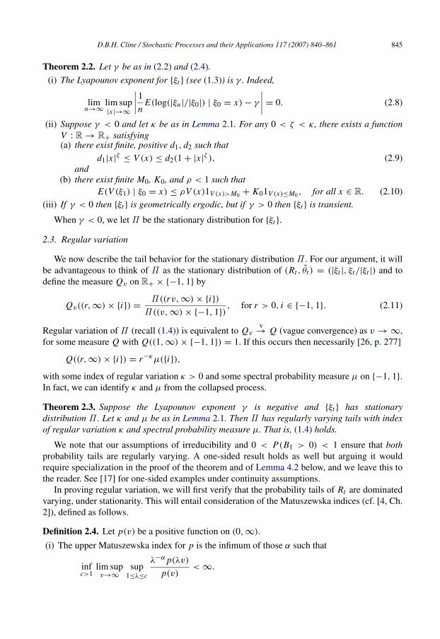
(ii) The lower Matuszewska index for p is the supremum of those β such that

supc>1

lim infv→∞

inf1≤λ≤c

λ−β p(λv)

p(v)> 0.

Since probability tails are nonincreasing, the indices will be nonpositive. More importantly,we will need to verify that they are finite, negative and equal. Although equality of theMatuszewska indices generally does not imply regular variation, it will in fact suffice for us.

3. Examples

3.1. Random coefficients model

Goldie [17] analyzes the tail behavior for the stationary distributions of models of the form

ξt = Btξt−1 + c(ξt−1, Bt , Ct ), (3.1)

where etdef= (Bt , Ct ) is an iid sequence in R2, c(·, B, C) is continuous for each (B, C) and

|c(x, B, C)| ≤ c(1 + |B| + |C |) for some finite c. An important special case, studied byKesten [22] and also by de Saporta [27], is the one-dimensional random coefficients model

ξt = Btξt−1 + Ct .

Model (3.1) is a special case of (1.1) with b(x, B, C) = sgn(x)B. There is no loss in allowinget to be multidimensional as long as our other assumptions are met. Those assumptions are notautomatic, however. For example, Ct = m(1 − Bt ) almost surely for some constant m leads to adegenerate stationary distribution for the random coefficients model (cf. [17]), but the model isnot irreducible. (See also [12].)

From (2.4), γ = E(log |b(±1, e1)|) = E(log |B1|). Verwaat [29] and Grincevicius [18] (forexample) showed that γ < 0 suffices for ergodicity. Likewise, from Lemma 2.1, the parameterκ satisfies E(|Bt |

κ) = 1 and µ1 = µ−1 =12 since mκ,−1,1 = 1 − mκ,1,1 = E(|Bt |

κ1Bt <0), inagreement with Goldie (under the assumption 0 < P(B1 > 0) < 1).

3.2. AR-ARCH model

The AR-ARCH model of order 1 is

ξt = a0 + a1ξt−1 + (b0 + b1ξ2t−1)

1/2et .

This is the model examined by Borkovec and Kluppelberg [7], under the additional assumptionthat et has a distribution symmetric about 0. The ordinary ARCH(1) model is a special casewith a1 = a0 = 0. If a1 6= 0, however, the combination of an autoregression term with theARCH term precludes the possibility of embedding it in a random coefficients model. We haveb(i, e1) = ia1 + b1/2

1 e1, i = ±1, so that

p−1,1 = P(−a1 + b1/21 e1 > 0) and p1,−1 = P(a1 + b1/2

1 e1 < 0).

From (2.4), the Lyapounov exponent is

γ =p1,−1 E(log |a1 − b1/2

1 e1|) + p−1,1 E(log |a1 + b1/21 e1|)

p1,−1 + p−1,1.


The index of regular variation, κ , solves (2.7) with

mκi j = E(|ia1 + b1/21 e1|

κ1 j (ia1+b1/21 e1)>0), i, j ∈ {−1, 1},

and the tail weights are given by

µ1 = 1 − µ−1 =

E(|a1 − b1/21 e1|

κ1a1−b1/21 e1<0)

1 − E(|a1 − b1/21 e1|κ1a1−b1/2

1 e1<0) + E(|a1 + b1/21 e1|κ1a1+b1/2

1 e1>0).

When e1 is assumed to have a symmetric distribution, the results simplify considerably. In this

case, |a1 − b1/21 e1|

D= |a1 + b1/2

1 e1| so that γ = E(log |a1 + b1/21 e1|), µ−1 = µ1 = 1/2 and κ

solves E(|a1 + b1/21 e1|

κ) = 1.When a0 = a1 = 0, we of course have the standard ARCH model. Here, γ = log b1/2

1 +

E(log |e1|), κ satisfies bκ/21 E(|e1|

κ) = 1 and µ1 = bκ/21 E(|e1|

κ1e1>0). Note that ξ2t satisfies

a random coefficients model. Goldie’s results would only determine the tail properties of |ξt |,whereas we also identify the tail weights.

3.3. Threshold AR-ARCH model

The results for the threshold model (1.2) are only slightly more involved. Here, we have

p−1,1 = P(−a11 + b1/211 e1 > 0) and p1,−1 = P(a31 + b1/2

31 e1 < 0).

The Lyapounov exponent is

γ =p1,−1 E(log |a11 − b1/2

11 e1|) + p−1,1 E(log |a31 + b1/231 e1|)

p1,−1 + p−1,1

and κ solves (2.7) with

mκ,−1, j = E(|a11 − b1/211 e1|

κ1 j (a11−b1/211 e1)<0), j ∈ {−1, 1},

and

mκ,1, j = E(|a13 + b1/213 e1|

κ1 j (a31+b1/231 e1)>0), j ∈ {−1, 1}.

Again, these quantities are used in (2.6) to compute µ1 and µ−1.For a threshold ARCH model (without the autoregression term), a11 = a31 = 0.

Consequently,

γ = p log b1/211 + (1 − p) log b1/2

31 + E(log |e1|),

where p = P(e1 < 0). Also, µ1 = E(|e1|

κ1e1>0)/E (|e1|

κ) and κ solves

bκ/211 E(|e1|

κ1e1<0) + bκ/231 E(|e1|

κ1e1>0) = 1.

Smooth transition models also fall within the framework here. Suppose G is a continuousprobability distribution function on R, with supx∈R |x |G(x)(1 − G(x)) < ∞, and

ξt = (a10 + a11ξt−1 + (b10 + b11ξ2t−1)

1/2et )(1 − G(ξt−1))

+ (a30 + a31ξt−1 + (b30 + b31ξ2t−1)

1/2et )G(ξt−1).


Then the above conclusions hold exactly as stated.

3.4. Random switching AR-ARCH model

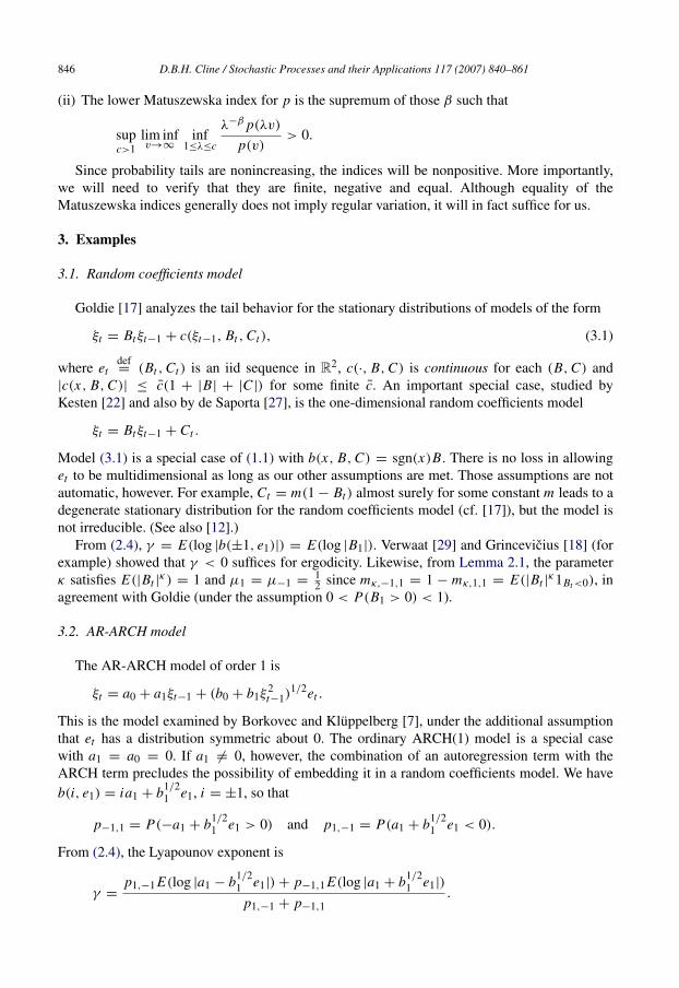
Our results allow for some nonlinearity in the errors. For example, regime switching could besignaled by the value (or sign) of the errors rather than by the time series itself. A simple examplethat satisfies our assumptions is

ξt = a0 + a1ξt−1 + (b0 + b1ξ2t−1)

1/2et G(et ) − (d0 + d1ξ2t−1)

1/2et G(−et ),

where again G is a continuous probability distribution function on R. Now b(i, e1) = ia1 +

b1/21 et G(et ) − d1/2

1 et G(−et ), i = ±1, and γ , κ and µ can be computed accordingly from (2.4)and Lemma 2.1.

4. Proofs

4.1. Showing ergodicity

Here we show that γ is in fact the Lyapounov exponent for {ξt } and that γ < 0 implies {ξt }

is geometrically ergodic. This argument is actually a much simpler version of the piggybackargument in Cline and Pu [13] where we dealt primarily with higher order AR-ARCH models.

Lemma 4.1. Let ν and γ be as in (2.3) and (2.4), respectively. Extend ν to R by ν(x) = ν(x/|x |)

if x 6= 0 and ν(0) = 0. Then

lim|x |→∞

E(

ν(ξ1) − ν(ξ0) + log(

1 + |ξ1|

1 + |ξ0|

) ∣∣∣∣ ξ0 = x)

= γ. (4.1)

Proof. By the definitions of ξt and θ∗t , if x = i |x |, i = ±1, then

|E(ν(θ∗

1 ) | θ∗

0 = i) − E(ν(ξ1) | ξ0 = x)| ≤ |ν(1)|P(η(i, e1) 6= a(x, e1)/|a(x, e1)|)

≤ |ν(1)|P(|c(x, e1)| > |b(x/|x |, e1)| |x |)

≤ |ν(1)|P(c(1 + |e1|) > |b(i, e1)| |x |). (4.2)

Obviously, therefore,

lim|x |→∞, x/|x |=i

|E(ν(θ∗

1 ) | θ∗

0 = i) − E(ν(ξ1) | ξ0 = x)| = 0. (4.3)

By Assumption A.3, E(| log W ∗

1 | | θ∗

0 = i) = E(| log(|b(i, e1)|)|) <∞. Also, Assumptions A.1and A.2 imply

E(

log(

1 + |b(i, e1)|x | + c(x, e1)|

1 + |x |

))≤ E (log (1 + |b(i, e1)| + |c(x, e1)|)) < ∞,

E(

log(

1 + |b(i, e1)x |/21 + |x |

))≥ E

(log (|b(i, e1)|/2) 1|b(i,e1)x |<2

)> −∞

and

E(

log(

1 + |b(i, e1)|x | + c(x, e1)|

1 + |b(i, e1)||x |/2

))≥ E(−log (1 + |b(i, e1)x |/2) 1|c(x,e1)|>|b(i,e1)x |/2)

≥ E(−log (1 + |c(x, e1)|)) > −∞.


Then easily by dominated convergence,

lim|x |→∞, x/|x |=i

E(

log(

1 + |ξ1|

1 + |ξ0|

) ∣∣∣∣ ξ0 = x)

= lim|x |→∞, x/|x |=i

E(

log(

1 + |b(i, e1)|x | + c(x, e1)|

1 + |x |

))= E(log b(i, e1)) = E(log W ∗

1 | θ∗

0 = i). (4.4)

The conclusion (4.1) follows from (2.2), (4.3) and (4.4). �

Proof of Theorem 2.2. (i) Fix L < ∞ arbitrarily. Observe that

lim sup|x |→∞

P(|ξ1| ≤ L | ξ0 = x) = lim sup|x |→∞

P(|a(x, e1)| ≤ L) = 0.

Let ε > 0 and choose L0 such that sup|x |>L0P(|ξ1| ≤ L | ξ0 = x) < ε. Thus,

lim sup|x |→∞

P(|ξt | ≤ L | ξ0 = x)

≤ lim sup|x |→∞

E(P(|ξt | ≤ L | ξt−1)1|ξt−1|>L0 | ξ0 = x) + lim sup|x |→∞

P(|ξt−1| ≤ L0 | ξ0 = x)

≤ ε + lim sup|x |→∞

P(|ξt−1| ≤ L0 | ξ0 = x).

Hence, inductively, for any L < ∞,

lim sup|x |→∞

P(|ξt | ≤ L | ξ0 = x) = 0, each t ≥ 1. (4.5)

Now let Bt = ν(ξt ) − ν(ξt−1) + log(1+|ξt |

1+|ξt−1|) for t ≥ 1. Fix ε > 0. From Lemma 4.1 we may

choose L1 such that

sup|x |>L1

|E(B1 | ξ0 = x) − γ | < ε.

Also, let

L2 = sup|x |≤L1

|E(B1 | ξ0 = x) − γ |.

Then, using (4.5),

lim sup|x |→∞

|E(Bt | ξ0 = x) − γ | ≤ lim sup|x |→∞

E(|E(Bt | ξt−1) − γ | | ξ0 = x)

≤ lim sup|x |→∞

E(ε1|ξt−1|>L1 + L21|ξt−1|≤L1 | ξ0 = x)

≤ ε + L2 lim sup|x |→∞

P(|ξt−1| ≤ L1 | ξ0 = x) ≤ ε.

Therefore, since ε is arbitrary,

lim sup|x |→∞

|E(Bt | ξ0 = x) − γ | = 0, each t ≥ 1. (4.6)

From (4.6) we thus have

lim sup|x |→∞

∣∣∣∣1n

E(

ν(ξn) − ν(ξ0) + log(

1 + |ξn|

1 + |ξ0|

)∣∣∣∣ ξ0 = x)

− γ

∣∣∣∣


≤1n

n∑t=1

lim sup|x |→∞

|E(Bt | ξ0 = x) − γ | = 0

and conclude

limn→∞

lim sup|x |→∞

∣∣∣∣1n

E(

log(

1 + |ξn|

1 + |ξ0|

)∣∣∣∣ ξ0 = x)

− γ

∣∣∣∣ = 0,

which is (2.8).(ii) This is similar to the proof of Lemma 4.1. For ζ < κ , define Mζ to be the matrix with

positive elements

mζ i jdef= E((W ∗

1 )ζ 1θ∗

1 = j | θ∗

0 = i), i, j ∈ {−1, 1}.

Let ρζ be the maximal eigenvalue with corresponding right eigenvector φ, which we interpret asa function on {−1, 1}. Note that φ is nonnegative. We will demonstrate in the proof of Lemma 2.1below that ρζ < 1. Define

V (x) =

{1 + φ(x/|x |)|x |

ζ , x 6= 0,

1, x = 0.

This function satisfies (2.9).Recall (4.2) and (4.3), which say in essence that

lim sup|x |→∞

P(η(i, e1) 6= a(x, e1)/|a(x, e1)|) = 0.

We similarly have

lim sup|x |→∞

E(|b(1, e1)|ζ 1η(i,e1)6=a(x,e1)/|a(x,e1)|) = 0.

Thus,

lim supx→∞

E(

V (ξ1)

V (ξ0)

∣∣∣∣ ξ0 = x)

= lim supx→∞

E(

φ(a(x, e1)/|a(x, e1)|)(|b(1, e1) |x | + c(x, e1)|ζ )

φ(1)|x |ζ

)=

φ(−1)

φ(1)E(|b(1, e1)|

ζ 1η(1,e1)<0) + E(|b(1, e1)|ζ 1η(1,e1)>0)

=φ(−1)

φ(1)mζ,1,−1 + mζ,1,1 = ρζ < 1. (4.7)

Likewise,

lim supx→−∞

E(

V (ξ1)

V (ξ0)

∣∣∣∣ ξ0 = x)

= ρζ < 1. (4.8)

Since E(V (ξ1) | ξ0 = x) is locally bounded as a function of x , (4.7) and (4.8) suffice to prove(2.10) with ρ ∈ (ρζ , 1).

(iii) From (2.8) and [11], γ > 0 implies |ξt | → ∞ in probability and thus that the process istransient.

Suppose instead that γ < 0. By Assumption A.4, {ξt } is irreducible with Lebesgue measureas a maximal irreducibility measure, is aperiodic and is a T -chain. Consequently, by Thm. 15.0.1of [24], (2.9) and (2.10) are sufficient to ensure {ξt } is geometrically ergodic. �


4.2. Showing regular variation

In this, the final and longest, subsection we assume {ξt } is stationary with negative Lyapounovexponent γ and distribution Π . Here, we will verify the regular variation of its probability tails.

We start by proving Lemma 2.1.

Proof of Lemma 2.1. Since, for any κ > 0, all the elements of Mκ are positive, it has anonnegative maximal eigenvalue ρκ and a unique left eigenvector µκ (µ′

κ Mκ = ρκµ′κ ) such

that µκ is a probability measure on {−1, 1}. We want to show that there is a unique κ > 0 suchthat ρκ = 1.

We first show that ρ1/κκ is strictly increasing in κ . To this end, let ζ > κ > 0 and define the

matrix Mζ accordingly. Let ρζ be the maximal eigenvalue for Mζ . Define pi j as in (2.1) and

dκi j =mκi j

pi j, dζ i j =

mζ i j

pi j.

Thus, there exists c < 1 such that

dκi j = E((W ∗

1 )κ | θ∗

0 = i, θ∗

1 = j)

< c(E((W ∗

1 )ζ | θ∗

0 = i, θ∗

1 = j))κ/ζ= c

(dζ i j

)κ/ζ, i, j ∈ {−1, 1}.

It follows that, for any probability measure µ and vector 1 =

(11

),

µ′Mnκ 1 =

∑il =±1

l=0,...,n

µi0

n∏l=1

pil−1il

n∏l=1

dκil−1il

< cn∑il =±1

l=0,...,n

µi0

n∏l=1

pil−1il

n∏l=1

(dζ il−1il )κ/ζ

< cn

∑il =±1

l=0,...,n

µi0

n∏l=1

pil−1il

n∏l=1

dζ il−1il

κ/ζ

= cn(µ′Mnζ 1)κ/ζ .

Hence,

ρκ = limn→∞

(µ′Mnκ 1)1/n

≤ c limn→∞

((µ′Mnζ 1)κ/ζ )1/n

= c(ρζ

)κ/ζ,

showing the strict monotonicity as desired.Now let E be the matrix with elements

ei j = exp(E((log W ∗

1 )1θ∗

1 = j | θ∗

0 = i)), i, j ∈ {−1, 1}.

and note that

limκ↓0

d1/κκi j = exp(E(log W ∗

1 | θ∗

0 = i, θ∗

1 = j)).

So, by an argument similar to the above, limκ↓0 ρ1/κκ is the maximal eigenvalue of E . Since

(exp(ν(−1))exp(ν(1))

) is a nonnegative eigenvector for E with corresponding eigenvalue eγ , by (2.2), it


must be that eγ is the maximal eigenvalue of E . Therefore, since γ < 0, ρκ must be less than1 for small enough κ . Also, ρκ clearly is continuous in κ and, by Assumptions A.1 and A.3,ρκ > 1 for large enough κ . From all this, it follows that there is a unique positive κ for whichρκ = 1. �

Lemma 4.2. Let κ and µ j , j = ±1, be the solution in Lemma 2.1 and set

Ti j (w) = P(W ∗

1 ≤ w, θ∗

1 = j | θ∗

0 = i).

Suppose q−1, q1 are nonnegative measurable functions on R+ such that

sup0<r≤1

rκ+δq j (r) < ∞ and supr≥1

rκ−δq j (r) < ∞, j = ±1,

for every δ > 0. Suppose also that they solve the system of equations

q j (r) =

∑i=±1

∫∞

0qi (r/w)Ti j (dw). (4.9)

and q−1(1) + q1(1) = 1. Then q j (r) = µ jr−κ .

Proof. Define g j (x) = eκx q j (ex ). By Assumption A.3, each Ti j is absolutely continuous withdensity, say, ti j . Define τi j (x) = eκx ti j (ex ). Then (4.9) becomes

g j (x) =

∑i=±1

∫∞

−∞

gi (y)τi j (x − y) dy, j = ±1, (4.10)

namely, a linear system of integral equations with a convolution kernel, subject to e−δ|x |g j (x), isbounded, j = ±1. By Assumptions A.1 and A.2, we also deduce that

∫∞

−∞eζ |x |τi j (x) dx < ∞

for all ζ, i, j . Expressing (4.10) more simply,

g−1 = g−1 ∗ τ−1,−1 + g1 ∗ τ1,−1 and g1 = g−1 ∗ τ−1,1 + g1 ∗ τ1,1.

We are thus justified in computing

g1 ∗ (1 − τ−1,−1) = g−1 ∗ (1 − τ−1,−1) ∗ τ−1,1 + g1 ∗ τ1,1 ∗ (1 − τ−1,−1)

= g1 ∗ τ1,−1 ∗ τ−1,1 + g1 ∗ τ1,1 ∗ (1 − τ−1,−1), (4.11)

or, equivalently, g1 = g1 ∗ σ , where

σ = τ−1,−1 + τ1,1 − τ−1,−1 ∗ τ1,1 + τ−1,1 ∗ τ1,−1.

Similarly, g−1 = g−1 ∗ σ . Let τ = {τi j } be the matrix of Fourier transforms for the τi j ’s. So

τi j (α) = E((W ∗

1 )κ+iα1θ∗

1 = j | θ∗

0 = i) and σ (α) = det(I − τ (α)). (4.12)

From classical results (e.g., Sec. 11.2 of [28]), the solutions to (4.11) are linear combinations ofeiαk x Pjk(x), where αk is a root of σ (α) = det(I − τ (α)) = 0 in the strip Im(α) < δ and Pjkis a polynomial of degree one less than the multiplicity of αk . Note that α = 0 is root, by (4.12)and Lemma 2.1, and it has multiplicity 1 because τ (0) = Mκ has a simple eigenvalue equal to1. Also, δ may be chosen arbitrarily small. Hence, the only nonnegative solutions to (4.10) areconstant functions which thus satisfy

g j =

∑i=±1

gi

∫∞

−∞

τi j (y) dy =

∑i=±1

gi mκi j .


By the conclusion of Lemma 2.1, and since g−1 + g1 = 1, g−1 and g1 must be equal to theelements of µ.

We conclude, then, that q j (r) = µ jr−κ gives the unique nonnegative solution to (4.9) subjectto q−1(1) + q1(1) = 1. �

The significance of the above result is in the next one, which essentially identifies the uniqueinvariant measure for the transient process {ξ∗

t } defined in (1.5). Observe that

P(|ξ∗t | > r, ξ∗

t /|ξ∗t | = i | |ξ∗

t−1| = s, ξ∗

t−1/|ξ∗

t−1| = θ)

= P(W ∗

1 > r/s, θ∗

1 = i | θ∗

0 = θ)

= P(w(θ, e1) > r/s, η(θ, e1) = i). (4.13)

Corollary 4.3. Let κ and µ j , j = ±1, be the solution in Lemma 2.1. Suppose Q is a measureon R+ × {−1, 1} satisfying Q((1, ∞) × {−1, 1}) = 1,

supr≤1

rκ+δ Q((r, ∞) × {i}) < ∞ and supr≥1

rκ−δ Q((r, ∞) × {i}) < ∞,

for every δ > 0, and

Q((r, ∞) × {i}) =

∫R+×{−1,1}

P(w(θ, e1) > r/s, η(θ, e1) = i)Q(dsdθ),

r > 0, i ∈ {−1, 1}. (4.14)

Then Q((r, ∞) × {i}) = µir−κ .

Proof. Let qi (r) = Q((r, ∞) × {i}). Then by (4.13) and a simple integration by parts, (4.14) isexactly the same as (4.9). �

We now turn to the tail behavior of the stationary distribution Π . It actually will be convenientto think of Π as the stationary distribution of {(Rt , θt )} = {(|ξt |, ξt/|ξt |)}.

A helpful alternative to Definition 2.4 is given by the following result (cf. [4], Thm. 2.2.2,or [1]).

Theorem 4.4 (Aljancic and Arandelovic). Let p(v) be a positive function on (0, ∞).

(i) The upper Matuszewska index for p is the infimum of those α such that there exist finite Kand v0 with

p(λv)

p(v)≤ Kλα, for λv ≥ v ≥ v0.

(ii) The lower Matuszewska index for p is the supremum of those β such that there exist finite Kand v0 with

p(λv)

p(v)≤ Kλβ , for v ≥ λv ≥ v0.

Lemma 4.5. Suppose {ξt } is stationary.

(i) Then P(Rt > v) is of dominated variation: its Matuszewska indices are finite.


(ii) Let −κL be the lower Matuszewska index for P(Rt > v). Then for any β > κL there existsK1 < ∞ and v0 < ∞ such that

P(R1 > λv)

P(R1 > v)≤ K1λ

−β , for v > λv ≥ v0. (4.15)

(iii) Additionally,

limv→∞

supx∈R

P(|c(x, e1)| > εv)

P(R1 > v)= 0, for all ε > 0. (4.16)

Proof. Recall Assumption A.2. We may assume b2 ≥ max(b1/2, 2) without any loss. Note that

R1 = |b(θ0, e1)R0 + c(θ0 R0, e1)| ≥ (b1|e1| − b2)R0 − c(1 + |e1|).

Let M1 = 8c/b1. Then R0 > M1 and |e1| ≥ 2b2/b1 ≥ 1 imply

R1 ≥ (b1|e1| − b2)R0 − c(1 + |e1|) ≥ R0(b1/2 − 2c/M1)|e1| ≥ R0b1|e1|/(2b2).

Let 0 < δ < 1. Given R1D= R0 and v > M1/δ, we have

P(R1 > v) ≥ P(R0 > δv, b1|e1| > 2b2/δ) = P(R1 > δv)P(b1|e1| > 2b2/δ).

Hence,

supv>M1/δ

P(R1 > δv)

P(R1 > v)≤ K2

def=

1

P(b1|e1| > 2b2/δ)< ∞, (4.17)

showing that R1 has dominated varying probability tail (cf. [4]).In particular, this means the probability tail has a finite (and nonpositive) lower Matuszewska

index, say −κL . From Theorem 4.4(ii) we find that for each β > κL , (4.15) must hold with somefinite K1. In particular (take λv = v0 in (4.15)), P(R1 > v) > δ0v

−β for some δ0 > 0. Takenwith Assumption A.2 and the fact E(|e1|

β) < ∞, this implies (4.16). �

Lemma 4.5 shows that the Matuszewska indices are finite. Lemma 4.7 below will show thatthey are in fact negative. Ultimately, they will turn out to be equal to each other.

Lemma 4.6. Assume as in Lemma 4.5. For any r > 0 and ε > 0, there exists δ > 0 and M2 < ∞

such thatP(R1 > rv, R0 < δv)

P(R0 > v)< ε, for all v > M2.

Proof. Let F1 be the distribution of 1 + |e1|. Suppose 0 < δ ≤ 1 and let β > κL . ByAssumption A.1 and Lemma 4.5, we know

limv→∞

P(|e1| > cv)

P(R1 > v)= 0, for any c > 0. (4.18)

Choose v0 as in (4.15) with v0 ≥ c/b. If v > v0/δ then, using (4.15),

P(R1 > rv, R0 < δv)

≤ P((bR0 + c)(1 + |e1|) > rv, R0 < δv)

≤ P(bR0(1 + |e1|) > rv/2, r/(2δb) ≤ 1 + |e1| ≤ rv/(2bv0))


+ P(1 + |e1| > rv/(2bv0))

=

∫ rv/(2bv0)

r/(2δb)

P(R0 > rv/(2bu)

)F1(du) + P(1 + |e1| > rv/(2br0))

≤ K1

∫ rv/(2bv0)

r/(2δb)

(2bu

r

)β

F1(du)P(R0 > v) + P(1 + |e1| > rv/(2bv0)). (4.19)

We may choose δ > 0 to make K1∫

∞

r/(2δb)( 2bu

r )β F1(du) < ε/2 and, by (4.18), we may chooseM2 > v0/δ so that

P(1 + |e1| > rv/(2bv0))

P(R0 > v)< ε/2, for all v > M2.

Combining these with (4.19) gives the result. �

Lemma 4.7. Suppose {ξt } is stationary with (2.9) and (2.10) holding. Let the stationarydistribution be Π .

(i) The upper Matuszewska index for P(Rt > v) is no bigger than −ζ .(ii) For each k ≥ 0, the measures Qk

v , v ≥ 1, given by

Qkv((r, ∞) × {i}) =

Π ((max(r, 2−k)v, ∞) × {i})Π ((v, ∞) × {−1, 1})

, r > 0, i ∈ {−1, 1}, (4.20)

are tight on R+ × {−1, 1}.

Proof. First, suppose k = 0. Note that Q0v is the conditional distribution of (Rt/v, θt ), given

Rt > v, under stationarity.By (2.9) and (2.10) and Assumption A.2,

V (ξ1) ≤ d2(|b(θ1, e1)ξ0| + |c(ξ0, e1)|)ζ

+ d2 ≤ d2(b|ξ0| + c)ζ (1 + |e1|)ζ

+ d2.

This implies the existence of finite, positive d3, d4 such that

V (ξ1) ≤ (d3V (ξ0) + d4)(1 + |e1|)ζ

+ d2.

Let K3 = E((1 + |e1|)ζ ). Then, if r > M0,

E(V (ξ1)1V (ξ1)>r ) = E(V (ξ1)1V (ξ1)>r,V (ξ0)>r ) + E(V (ξ1)1V (ξ1)>r,V (ξ0)≤r )

≤ E(E(V (ξ1) | ξ0)1V (ξ0)>r )

+ E(((d3r + d4)(1 + |e1|)ζ

+ d2)1V (ξ1)>r )

≤ ρE(V (ξ0)1V (ξ0)>r ) + ((d3r + d4)K3 + d2)P(V (ξ1) > r).

Under stationarity, V (ξ1)D= V (ξ0), and E(V (ξ0)) < ∞ by Meyn and Tweedie [24, Thm. 14.0.1].

Hence

1r

E(V (ξ1) | V (ξ1) > r) =E(V (ξ1)1V (ξ1)>r )

r P(V (ξ1) > r)

≤ ρE(V (ξ1)1V (ξ1)>r )

r P(V (ξ1) > r)+ d3 K3 + (d4 K3 + d2)/M0. (4.21)


It follows from (4.21) that

supr>M0

1r

E(V (ξ1) | V (ξ1) > r) ≤ K4def=

d3 K3 + (d4 K3 + d2)/M0

1 − ρ< ∞. (4.22)

Furthermore, we have d1 Rζ0 ≤ V (ξ0) ≤ d2(1 + Rζ

0 ). Thus,

E(Rζ0 1Rζ

0 >r ) ≤1d1

E(V (ξ0)1V (ξ0)>d1r ) (4.23)

and, if d1r > 2d2,

P(Rζ0 > d1r/(2d2)) ≥ P(V (ξ0) > d1r). (4.24)

Let δ = (d1/(2d2))1/ζ and obtain M1, K2 from the proof of Lemma 4.5. Set

r0 = max(M0, 2d2, 2d2 Mζ1 )/d1.

Then, by (4.17) and (4.22)–(4.24), we obtain

supv>r1/ζ

0

∫∞

1

∫{−1,1}

sζ Q0v(dsdθ) = sup

r>r0

1r

E(Rζ0 | Rζ

0 > r)

= supr>r0

P(Rζ0 > d1r/(2d2))

P(Rζ0 > r)

E(Rζ0 1Rζ

0 >r )

r P(Rζ0 > d3r/(2d4))

≤ K2 supr>r0

1d1r

E(V (ξ1) | V (ξ1) > d1r)

≤ K2 K4 < ∞. (4.25)

This is sufficient for the probability measures {Q0v}v≥1 to be tight on R+ × {−1, 1}.

Indeed, from (4.25), we easily determine that

P(R0 > λv)

P(R0 > v)≤ K2 K4λ

−ζ , λv ≥ v ≥ r1/ζ

0 .

Hence, the upper Matuszewska index is no more than −ζ .Let ε1 > 0. By the above we can choose M3 ∈ [1, ∞) so that Qk

v((M3, ∞) × {−1, 1}) =

Q0v((M3, ∞) × {−1, 1}) < ε1, for all v ≥ r1/ζ

0 , k ≥ 1. This proves the tightness of {Qkv}v≥1 on

R+ × {−1, 1} for each k. �

In fact, assuming γ < 0, we may choose any ζ < κ , by Theorem 2.2(ii). This implies that theupper Matuszewska index is no more than −κ , but is still some way from saying Π is regularlyvarying or even that the two indices are equal.

Next is the lemma that is at the heart of our proof. Recall the definition of Qv in (2.11).

Lemma 4.8. Assume as in Lemma 4.7. For any sequence vn → ∞, there exists a sub-sequence vn → ∞ and a continuous measure Q on R+ × {−1, 1} such that Qvn

v→ Q,

Q((1, ∞) × {−1, 1}) = 1 and

Q((r, ∞) × {i}) =

∫R+×{−1,1}

P(w(θ, e1) > r/s, η(θ, e1) = i)Q(dsdθ), (4.26)

for i ∈ {−1, 1}, r > 0.


Proof. Let Qkv , v ≥ 1, be as in (4.20), namely the restriction of Qv to (2−k, ∞) × {−1, 1}.

Note that, by (4.17) for each k, the measures Qkv are uniformly bounded. By Lemma 4.7, the

probability measures Q0v are tight on R+ × {−1, 1}. Given any sequence vn → ∞, there

exists a subsequence v0n → ∞ and a measure Q0 such that Q0

v0n

v→ Q0 and, of course,

Q0((1, ∞) × {−1, 1}) = 1. Iteratively we may find a further subsequence vkn → ∞ and a

measure Qk such that Qkvk

n

v→ Qk and Qk agrees with Qk−1 on (21−k, ∞) × {−1, 1}. Letting

vn = vnn , we have Qvn

v→ Q where Q is a measure that agrees with Qk on (2−k, ∞) × {−1, 1}

for each k. At this point we do not know that Q is continuous.Note that w(θ0, e1)R0 > (1 + ε/2)v implies either R1 > v or |c(θ0 R0, e1)| > εv/2. Thus,

P(R1 > v, θ1 = i | R0 = s, θ0 = θ)

≥ P(w(θ, e1) > (1 + ε/2)v/s, η(θ, e1) = i) − P(|c(θs, e1)| ≥ εv/2). (4.27)

Using (4.27) and (4.16),

lim infn→∞

Qvn ((r, ∞) × {i}) = lim infn→∞

P(R1 > rvn, θ1 = i)P(R0 > vn)

≥ lim infn→∞

∫R+×{−1,1}

P(R1 > rvn, θ1 = i | R0 = s, θ0 = θ)

×1(2−kvn ,∞)(s)Π (dsdθ)

Π ((vn, ∞) × {−1, 1})

= lim infn→∞

∫R+×{−1,1}

P(R1 > rvn, θ1 = i | R0 = vns, θ0 = θ)

×Qkvn

(dsdθ)

≥ lim infn→∞

∫R+×{−1,1}

P(w(θ, e1) > (1 + ε/2)r/s, η(θ, e1) = i)

×Qkvn

(dsdθ).

By Assumption A.3, P(w(θ, e1) > ·, η(θ, e1) = ·) is continuous in R+ × {−1, 1}. It follows bystandard theory for vague convergence (e.g., [2, Thm. 4.5.1]) that

lim infn→∞

Qvn ((r, ∞) × {i})

≥

∫R+×{−1,1}

P(w(θ, e1) > (1 + ε/2)r/s, η(θ, e1) = i)Qk(dsdθ).

By monotone convergence, as k ↑ ∞ and ε ↓ 0,

lim infn→∞

Qvn ((r, ∞) × {i}) ≥

∫R+×{−1,1}

P(w(θ, e1) > r/s, η(θ, e1) = i)Q(dsdθ). (4.28)

Fix m ≥ 0. Let ε1 > 0 be chosen arbitrarily. By Lemma 4.6, with r = 2−m , we may chooseδ = 2−k to make

lim supn→∞

P(R1 ≥ 2−mvn, R0 < 2−kvn)

Π ((vn, ∞) × {−1, 1})< ε1.


Then, again using (4.16) and [2, Thm. 4.5.1],

lim supn→∞

Qvn ([2−m, ∞) × {−1, 1})

≤ lim supn→∞

∫R+×{−1,1}

P(R1 ≥ 2−mvn | R0 = s, θ0 = θ)1[2−kvn ,∞)(s)

×Π (dsdθ)

Π ((vn, ∞) × {−1, 1})

+ lim supn→∞

P(R1 ≥ 2−mvn, R0 < 2−kvn)

Π ((vn, ∞) × {−1, 1})

≤ lim supn→∞

∫R+×{−1,1}

P(R1 ≥ 2−mvn | R0 = vns, θ0 = θ)Qkvn

(dsdθ) + ε1

≤ lim supn→∞

∫R+×{−1,1}

P(w(θ, e1) > (1 − ε/2)2−m/s)Qkvn

(dsdθ) + ε1

=

∫R+×{−1,1}

P(w(θ, e1) > (1 − ε/2)2−m/s)Qk(dsdθ) + ε1.

Dominated convergence as ε ↓ 0 and monotone convergence as k ↑ ∞ yields

lim supn→∞

Qvn ([2−m, ∞) × {−1, 1}) ≤

∫R+×{−1,1}

P(w(θ, e1) ≥ 2−m/s)Q(dsdθ) + ε1.

The arbitrary choice of ε1 finally gives

lim supn→∞

Qvn ([2−m, ∞) × {−1, 1}) ≤

∫R+×{−1,1}

P(w(θ, e1) ≥ 2−m/s)Q(dsdθ). (4.29)

Since P(w(θ, e1) = 2−m/s) = 0 for all s > 0, (4.29) combined with (4.28) for r = 2−m implies

limn→∞

Qvn ([2−m, ∞) × {−1, 1}) =

∫R+×{−1,1}

P(w(θ, e1) ≥ 2−m/s)Q(dsdθ). (4.30)

From (4.28) and (4.30), we can now conclude that the measures Qmvn

converge vaguely, once

again by Ash [2, Thm. 4.5.1]. Therefore, in fact Qvnv

→ Q, where Q is continuous and definedby

Q((r, ∞) × {i}) =

∫R+×{−1,1}

P(w(θ, e1) > r/s, η(θ, e1) = i)Q(dsdθ).

Finally, since also Qvnv

→ Q, it must be that Q = Q and (4.26) holds. �

Lemma 4.9. Let Q be a vague subsequential limit of Qv , as in Lemma 4.8. Then

either infr>0

Q((r, ∞) × {−1})

Q((r, ∞) × {−1, 1})> 0 or inf

r>0

Q((r, ∞) × {1})

Q((r, ∞) × {−1, 1})> 0. (4.31)

Proof. Let ∆−1 and ∆1 be as in Assumption A.3 and assume ∆1 > 0. Choose r0 such thatP(b(θ, e1) > r) ≥

∆12 P(|b(θ, e1)| > r) for all r ≥ r0. Let δ = min(

∆12 , P(b(θ, e1) > r0)).

Then

P(b(θ, e1) > r/s) ≥ δP(|b(θ, e1)| > r/s), for all r > 0, s ≤ r/r0,


and

P(b(θ, e1) > r/s) ≥ P(b(θ, e1) > r0) ≥ δP(|b(θ, e1)| > r/s), for all r > 0, s ≥ r/r0.

Note that b(θ, e1) > r iff w(θ, e1) > r and η(θ, e1) = 1. Thus, from (4.26),

Q((r, ∞) × {1}) =

∫R+×{−1,1}

P(b(θ, e1) > r/s)Q(dsdθ)

≥ δ

∫R+×{−1,1}

P(|b(θ, e1)| > r/s)Q(dsdθ) = δQ((r, ∞) × {−1, 1}).

This shows that the second inequality in (4.31) holds if ∆1 > 0. A similar argument applies toshow that the first inequality in (4.31) holds if ∆−1 > 0. �

Finally, we are ready to prove our principal result.

Proof of Theorem 2.3. Let −κL ≤ −κU be the lower and upper Matuszewska indices,respectively, for the function p(r) = P(Rt > r) under stationarity. From Lemmas 4.5 and4.7 we know they are finite and negative. Before we can proceed further, we need to show thatthese indices are both equal to κ . This will require several steps. First, let Qvn be a sequenceconverging vaguely to Q, as in Lemma 4.8. Let α > −κU . By Theorem 4.4,

Q((λr, ∞) × {−1, 1})

Q((r, ∞) × {−1, 1})= lim

n→∞

P(Rt > λrvn)

P(Rt > rvn)≤ Kλα, (4.32)

for some finite K and all λ ≥ 1. Consequently, the upper Matuszewska index for q(r) =

Q((r, ∞) × {−1, 1}) is no more than −κU . Likewise, the lower Matuszewska index for q(r)

is no less than −κL . This is true for any vague subsequential limit Q.Next, we apply the Polya peak theorem (Thm. 2.5.2 in [4], from [16]): there exists a sequence

vn → ∞ such that

lim supn→∞

Qvn ((r, ∞) × {−1, 1}) = lim supn→∞

P(Rt > r vn)

P(Rt > vn)≤ r−κL , for all r > 0. (4.33)

From Lemma 4.8, there is a subsequence vn → ∞ and a continuous measure Q such thatQvn

v→ Q. Define the upper and lower orders for q(r) = Q((r, ∞) × {−1, 1}) by

ωL = lim infr→∞

log q(r)

log rand ωU = lim sup

r→∞

log q(r)

log r.

Hence, ωL ≤ ωU ≤ −κL , by (4.33). From Prop. 2.2.5 of [4] and our comment above aboutthe lower Matuszewska index for q(r), ωL ≥ −κL also. Thus, ωL = −κL . Therefore, by Thm.2.3.11 (note the misprint) of [4] and the continuity of Q, there exists a function g(r) which isregularly varying on R+ with index −κL such that lim infr→∞ Q((r, ∞) × {−1, 1})/g(r) = 1.Define

qi = lim infr→∞

Q((r, ∞) × {i})g(r)

, i = ±1. (4.34)

Both q−1 and q1 are finite and at least one is positive by Lemma 4.9 (critical points that havecompelled us to this intricate, nested argument of indices and orders).


Recall that Q satisfies (4.26). Letting Ti j (w) = P(W ∗

1 ≤ w, θ∗

1 = j | θ∗

0 = i), (4.26) may bereexpressed as

Q((r, ∞) × { j}) =

∑i=±1

∫∞

0Q((r/w, ∞) × {i}) Ti j (dw). (4.35)

From (4.34) and (4.35) and the regular variation of g(r) we get

q j ≥

∑i=±1

∫∞

0lim infr→∞

Q((r/w, ∞) × {i})g(r/w)

g(r/w)

g(r)Ti j (dw)

=

∑i=±1

∫∞

0qiw

κL Ti j (dw) =

∑i=±1

qi mκL i j ,

where mκL i j is defined by (2.5). This means the maximal eigenvalue of the matrix MκL =

[mκL i j ]i j is no larger than 1. That, in turn, implies κL ≤ κ by the proof of Lemma 2.1. A similarargument (or the comment following the proof of Lemma 4.7) confirms κU ≥ κ . But κL ≥ κU .Therefore, κL = κU = κ .

The point to all this is that we may now claim that for all δ > 0 (see (4.32) with r = 1 andα = −κ + δ),

supλ≥1

λκ−δ Q((λ, ∞) × { j}) < ∞

for any vague subsequential limit Q. Likewise, Theorem 4.4 also yields

supλ≤1

λκ+δ Q((λ, ∞) × { j}) < ∞,

for all δ > 0. We therefore have the conditions of Corollary 4.3 fulfilled so that the uniquesolution to (4.35) (and thus to (4.26)), subject to Q((1, ∞) × {−1, 1}) = 1, is given byQ((r, ∞) × {i}) = µir−κ . Since this true for any vague subsequential limit, we conclude thatQv

v→ Q, and therefore Π has regularly varying tails. �

References

[1] S. Aljancic, D. Arandelovic, O-regularly varying functions, Publications de l’Institut Mathematique, Belgrade(nouvelle serie) 22 (36) (1977) 5–22.

[2] R.B. Ash, Real Analysis and Probability, Academic Press, 1972.[3] B. Basrak, R. Davis, T. Mikosch, Regular variation of GARCH processes, Stochastic Process Appl. 99 (2002)

95–115.[4] N.H. Bingham, C.M. Goldie, J.L. Teugels, Regular Variation, Cambridge University Press, 1987.[5] M. Borkovec, Extremal behavior of the autoregressive process with ARCH(1) errors, Stochastic Process Appl. 85

(2000) 189–207.[6] M. Borkovec, Asymptotic behavior of the sample autocovariance and autocorrelation function of the AR(1) process

with ARCH(1) errors, Bernoulli 7 (6) (2001) 847–872.[7] M. Borkovec, C. Kluppelberg, The tail of the stationary distribution of an autoregressive process with ARCH(1)

errors, Ann. Appl. Probab. 11 (2001) 1220–1241.[8] P. Bougerol, N. Picard, Strict stationarity of generalized autoregressive processes, Ann. Probab. 20 (1992)

1714–1730.[9] P. Bougerol, N. Picard, Stationarity of GARCH processes and some nonnegative time series, J. Econom. 52 (1992)

115–127.[10] D.B.H. Cline, H.H. Pu, Verifying irreducibility and continuity of a nonlinear time series, Statist. Probab. Lett. 40

(1998) 139–148.[11] D.B.H. Cline, H.H. Pu, Geometric transience of nonlinear time series, Statist. Sinica 11 (2001) 273–287.


[12] D.B.H. Cline, H.H. Pu, A note on a simple Markov bilinear stochastic process, Statist. Probab. Lett. 56 (2002)283–288.

[13] D.B.H. Cline, H.H. Pu, Stability and the Lyaponouv exponent of threshold AR-ARCH models, Ann. Appl. Probab.14 (2004) 1920–1949.

[14] R.A. Davis, T. Mikosch, The sample autocorrelations of heavy-tailed processes with applications to ARCH, Ann.Statist. 26 (1998) 2049–2080.

[15] J. Diebolt, D. Guegan, Tail behaviour of the stationary density of general non-linear autoregressive processes oforder 1, J. Appl. Probab. 30 (1993) 315–329.

[16] D. Drasin, D.F. Shea, Polya peaks and the oscillation of positive functions, Proc. Amer. Math. Soc. 34 (1972)403–411.

[17] C.M. Goldie, Implicit renewal theory and tails of solutions of random equations, Ann. Appl. Probab. 1 (1991)126–166.

[18] A.K. Grincevicius, A random difference equation, Lithuanian Math. J. 20 (1981) 279–282.[19] D. Guegan, J. Diebolt, Probabilistic properties of the β-ARCH model, Statist. Sinica 4 (1994) 71–87.[20] H. Hult, F. Lindskog, Extremal behavior of regularly varying stochastic processes, Stochastic Process Appl. 115

(2005) 249–274.[21] H. Hult, F. Lindskog, T. Mikosch, G. Samorodnitsky, Functional large deviations for multivariate regularly varying

random walks, Ann. Appl. Probab. 15 (2006) 2651–2680.[22] H. Kesten, Random difference equations and renewal theory for products of random matrices, Acta Math. 131

(1973) 207–248.[23] C. Kluppelberg, P. Pergamenchtchikov, The tail of the stationary distribution of a random coefficient AR(q) model,

Ann. Appl. Probab. 14 (2004) 971–1005.[24] S.P. Meyn, R.L. Tweedie, Markov Chains and Stochastic Stability, Springer-Verlag, London, 1993.[25] T. Mikosch, C. Starica, Limit theory for the sample autocorrelations and extremes of a GARCH(1,1) process, Ann.

Statist. 28 (2000) 1427–1451.[26] S.I. Resnick, Extreme Values, Regular Variation and Point Processes, Springer-Verlag, 1987.[27] B. de Saporta, Tail of the stationary solution of the stochastic equation Yn+1 = anYn + bn with Markovian

coefficients, Stochastic Process Appl. 115 (2005) 1954–1978.[28] E.C. Titchmarsh, Introduction to the Theory of Fourier Integrals, 2nd ed., Oxford University Press, 1948.[29] W. Verwaat, On a stochastic difference equation and a representation of non-negative infinitely divisible random

variables, Adv. Appl. Prob. 11 (1979) 750–783.[30] Z. Zhang, H. Tong, A note on stochastic difference equations and its application to GARCH models, Chinese J.

Appl. Probab. Statist. 20 (2004) 259–269.

Documents

Regular variation of order 1 nonlinear AR-ARCH modelsdcline/Papers/nsrscalar.pdf · Regular variation of order 1 nonlinear AR-ARCH models Daren B.H. Cline ... nonlinearARCHandAR-ARCHmodels.Theresultshereareprecise,asopposedtothestronger