arX

iv:n

lin/0

6090

24v1

[nl

in.C

D]

11

Sep

2006

Regularity Properties of Critical Invariant Circles

of Twist Maps, and Their Universality

Arturo Olvera1∗ Nikola P. Petrov2†

September 14, 2018

1 IIMAS-UNAM, FENOMEC, Apdo. Postal 20–726, Mexico D. F. 01000, Mexico

2 Department of Mathematics, University of Oklahoma, Norman, OK 73019, USA

Abstract

We compute accurately the golden critical invariant circles of several area-preservingtwist maps of the cylinder. We define some functions related to the invariant circle andto the dynamics of the map restricted to the circle (for example, the conjugacy betweenthe circle map giving the dynamics on the invariant circle and a rigid rotation on thecircle). The global Holder regularities of these functions are low (some of them are noteven once differentiable). We present several conjectures about the universality of theregularity properties of the critical circles and the related functions. Using a Fourieranalysis method developed by R. de la Llave and one of the authors, we computenumerically the Holder regularities of these functions. Our computations show that– withing their numerical accuracy – these regularities are the same for the differentmaps studied. We discuss how our findings are related to some previous results: (a)to the constants giving the scaling behavior of the iterates on the critical invariantcircle (discovered by Kadanoff and Shenker); (b) to some characteristics of the singularinvariant measures connected with the distribution of iterates. Some of the functionsstudied have pointwise Holder regularity that is different at different points. Our resultsgive a convincing numerical support to the fact that the points with different Holderexponents of these functions are interspersed in the same way for different maps, whichis a strong indication that the underlying twist maps belong to the same universalityclass.

∗E-mail: aoc@uxmym1.iimas.unam.mx†E-mail: npetrov@ou.edu

1

Area-preserving twist maps of the cylinder are popular models of the dy-namics of many physical systems, i.e., they occur as Poincare maps of 2-degree-of-freedom Hamiltonian systems. Homotopically non-trivial invariant circles ofsuch a map play an important role in organizing the global dynamics of themap. Generally, as the perturbation grows, more and more of these circles aredestroyed, until there remains only one such circle, called the “critical” circle.This circle is the last obstacle to the unbounded growth of the “action variable”.In this critical situation many characteristics of the system become drasticallydifferent from the “under-critical” case. For example, consider the dynamics ofthe iterates of the twist map restricted to the critical circle – it is given by amap of the circle. This map can be conjugated to a rigid rotation on the circle,but the conjugating function has very low regularity – its Holder exponent islower than 1. The Holder regularity of this conjugacy is related to some uni-versal properties of the map, i.e., to the universal rescaling factors [1, 2] andto the scaling properties [3] of the distribution of the iterates on the criticalcircle (which is governed by a singular invariant measure). We compute severalfunctions related to the critical circle and to the dynamics on it and us a methoddeveloped in [4] to assess numerically their global Holder regularity. Our find-ings lend support to several conjectures concerned with the universality and therenormalization group description of these critical objects.

1 Introduction

It has been known since the late 1970’s and early 1980’s that many objects at the boundary ofchaotic behavior exhibit remarkable scaling properties and that, furthermore, these proper-ties are “universal”. Such properties are exhibited by unimodal maps of the interval [5, 6, 7],critical maps of the circle [8], critical KAM tori [1, 2], and other systems. These observationswere explained in terms of a renormalization group analysis, following a methodology thathad been developed earlier in the study of critical phenomena in statistical mechanics andfield theory [9, 10, 11, 12].

The scale invariance of the critical objects affects many of their properties. Notably, theHolder regularity of the critical objects (or some functions related to them) tends to have alow and fractional value. Presumably the values of the regularities are related to exponentsand geometric properties of the renormalization group fixed points which describe the criticalobjects.

Furthermore, the observation that critical objects can be divided in “universality classes”such that all objects in a given class “look the same” can be tested numerically. One way todo this is to define certain functions related to the critical objects – typically these functionsare not very regular (in some cases not even once differentiable), and to test numericallywhether the regularities of these functions are the same for different objects. Another – evenmore sensitive – test for universality is to take two functions, say h1 and h2, from the same

2

class, and to study the regularity of functions like h1 ◦ h−12 – for h1 and h2 belonging to

the same universality class, one can expect that h1 ◦ h−12 be more regular than h1 and h−1

2 .These ideas were tested in [4] in the case of non-critical and critical (with different degreeof criticality) circle maps, in which the empirical results are accompanied by an extensivemathematical theory. A substantial part of the effort in [4] was to develop implementationsof methods known in harmonic analysis (finite differences, Littlewood-Paley theory, waveletanalysis) to assess the regularity of the objects numerically.

In the present paper, we extend the methodology of [4] to the study of critical invariantcircles of area-preserving twist maps. Invariant circles in dynamical systems are amongthe most important objects that organize the long-term behavior of the system, and thecritical ones are especially important because of their role as “last barriers to chaos” (forreadable reviews see, e.g., [13], or, with more emphasis on the mathematical aspects, therecent book [14]). Critical invariant circles have been extensively studied since early 1980’s[1, 2, 15, 12].

We compute accurately the golden critical invariant circles of several standard-like area-preserving twist maps and some functions related to the dynamics of the iterates of the mapson these circles. Then we apply methods developed in [4] to study the Holder regularity ofthese functions and some universality aspects.

In Sec. 2 we give some background on twist maps and their critical invariant circles,define the functions that are the objects of our numerical study, and present several preciseconjectures concerning the properties of the critical invariant circles and the functions intro-duced. Sec. 3 is devoted to a discussion of the numerical methods used to compute criticalinvariant circles and to assess Holder regularity of functions. We collect our results in Sec. 4,and in Sec. 5 we discuss their significance and relationship with previous studies.

2 Critical invariant circles of twist maps

2.1 Twist maps

Let T := R/Z stand for the circle. We will be concerned with maps F of the (infinite)cylinder T× R,

F : T× R → T× R : (θ, r) 7→ F (θ, r) =: (θ′, r′) ,

which satisfy the following properties:

• Area preservation: The map F preserves the oriented area: detDF = 1.

• Zero-flux: The oriented area between a homotopically non-trivial circle and its imageunder F is 0. (In our situation, this is equivalent to saying that every non-trivial circleintersects its image.)

• Twist condition: For any fixed value of θ, ∂θ′

∂r> 0.

3

A map of the cylinder can be identified with a map F : R2 → R2 (called a lift of F )which satisfies

F (θ + 1, r) = F (θ, r) + (1, 0) .

Often one does not need to keep the distinction.The maps which we will use in our numerical studies are of the form (θ′, r′) := F (θ, r)

with

θ′ = (θ + r′) mod 1 ,(1)

r′ = r + λ V (θ) ,

where λ is a parameter, and V : T → R is a function satisfying∫ 1

0V (θ) dθ = 0. In particular,

many numerical studies have been devoted to studying (1) with

V (θ) = − 1

2πsin 2πθ , (2)

in which case we will call the map F the Taylor-Chirikov map.Given an orbit X = {(θn, rn) = F n(θ0, r0) |n = 0, 1, 2, . . .}, we define its rotation number,

ρ(X ), as the limit

ρ(X ) := limn→±∞

θn − θ0n

,

whenever this limit exists. In contrast with the situation for circle maps, the rotation numberdepends on the orbit (and it may happen that some orbits do not have rotation number).

We say that an orbit is well-ordered when for every k and l, the function of n defined ase(n) = θn+k − l− θn has the same sign. Every well-ordered orbit has a rotation number (theconverse, however, is not true).

It is also easy to see that if a bounded orbit is well-ordered and ρ(θ0, r0) is irrational,the closure of the orbit, {(θn, rn)}∞n=0, is a perfect set (i.e., every point is an accumulationpoint of points in the set); in other words, in this case the orbit is either a homotopicallynon-trivial circle or a Cantor set.

A set U ⊆ T× R is invariant if U = F (U).The following result plays an important role.

Theorem 2.1. If F is as above, for every ρ ∈ R there exists a well-ordered orbit withrotation number ρ.

2.2 Invariant circles of twist maps – rigorous results

The proof of the following theorem can be found in [16], [17]. We refer to [14] and [18] for adetailed exposition.

Theorem 2.2. Let U be an open simply connected invariant set, containing one of the endsof the cylinder. Then the boundary, ∂U , of the set U is an invariant circle which is the graph

4

of a Lipschitz function. In other words, ∂U can be written as r = R(θ), where R : T → R isa Lipschitz function.

For the map (1), the Lipschitz constant of the function R can be bounded by an expres-sion which involves only the Lipschitz constant of the function F in a neighborhood of thecircle ∂U .

In particular,

Corollary 2.1. Any homotopically non-trivial invariant circle is the graph of a Lipschitzfunction R. In the particular case of the map (1), the Lipschitz constant of R can be boundedby a constant which is independent of λLipV .

A number ρ is said to be Diophantine if, for each m,n ∈ N \ {0}, for some C > 0, andfor some d > 2, it satisfies ∣∣∣ρ− m

n

∣∣∣ >C

nd.

In the case when the map F is close to integrable and its rotation number ρ is Diophantine,one can apply Kolmogorov-Arnold-Moser theory to obtain that there exists an analyticinvariant circle such that the orbits on it have rotation number ρ.

Golden invariant circles are those with rotation number equal to the golden mean,

σG := [1, 1, 1, . . .] =

√5− 1

2. (3)

Here we have used the notation ρ = [a1, a2, a3, . . .] = 1/(a1 + 1/(a2 + 1/(a3 + · · · ))) for thecontinued fraction expansion of ρ ∈ (0, 1) [19].

There are also rigorous results that guarantee the non-existence of invariant circles of Fof the form (1).

Theorem 2.3. (i) If supθ |λ V (θ)| > 1, then (1) has no invariant circles.

(ii) If supθ |V ′(θ)| = 1 (which holds for the function (2)), then for |λ| > 43the map (1) has

no invariant circles.

(iii) For V given by (2), the map (1) has no golden invariant circles for |λ| > 6364

=0.984375 . . ..

(iv) For V given by (2), the map (1) has no golden invariant circles for |λ| > 0.9718.

Part (i) of Theorem 2.3 is elementary: if λ supθ |V (θ)| > 1, then there will exist points(θ∗, r∗) ∈ T × R such that F (θ∗, r∗) = (θ∗, r∗ + 1), which, iterated, gives that F n(θ∗, r∗) =(θ∗, r∗ + n) – the unbounded growth of the second coordinate of F n(θ∗, r∗) with n impliesthat a topologically non-trivial invariant circle cannot exist.

Part (ii) can be found in [17], parts (iii) and (iv) are proved by computer-assisted methodsin [20] and [21], resp.

It is widely believed that

5

Conjecture 2.1. For a Diophantine number ρ and for a map F of the form (1), there is anumber Λ(ρ) such that when |λ| > Λ(ρ), there is no invariant circle with rotation number ρ,and when |λ| < Λ(ρ), there exists an analytic invariant circle with rotation number ρ. Theinvariant circle becomes critical when |λ| = Λ(ρ).

Since our paper is devoted to homotopically non-trivial invariant circles, we will usuallyomit the words “homotopically non-trivial”.

2.3 Functions related to the critical invariant circles

We are interested in describing the critical invariant circles with rotation number ρ whichare in the boundary of existence. Postponing for the moment issues on how these objectscan be actually computed, we point out that to a given critical invariant circle γ of rotationnumber ρ, we can associate:

• the function R : T → R such that the critical invariant circle γ is the graph of R:

γ = {(θ, r) ∈ T× R : r = R(θ)} ; (4)

• the advance map g : T → T defined by

F (θ, R(θ)) = (g(θ), R ◦ g(θ)) ; (5)

• the hull map Ψ : T → T × R, which gives a representation of the invariant circle γ insuch a way that the dynamics on γ becomes a rotation by ρ, i.e.,

F ◦Ψ(θ) = Ψ(θ + ρ) ; (6)

• the map h = π1 ◦ Ψ : T → T (where π1 : T× R → T is the projection onto T), whichconjugates the advance map to a rotation by ρ:

g ◦ h(θ) = h(θ + ρ) ; (7)

• the map h−1 : T → T, which is the inverse of the map h defined in (7).

We note the following rigorous results.Theorem 2.2 guarantees that the invariant circle the function R is Lipschitz. It is an easy

consequence of the implicit function theorem that g should be as regular as R. Nevertheless,it is useful to compute the regularities of both g and R independently to asses the reliabilityof the numerical methods used.

Because of (7), it is clear that the regularity of g is not smaller than the minimum of theregularities of h and h−1.

6

2.4 The “big” conjugacies

Let ρ be a Diophantine number, Fi (i = 1, 2) be area-preserving twist maps, and γi bethe critical invariant circle of Fi with rotation number ρ. Let gγi and hγi be the associatedadvance map (5) and conjugacy (7), resp. We introduce the conjugating functions

Gγ1,γ2 := gγ1 ◦ g−1γ2

: T → T ,

Hγ1,γ2 := hγ1 ◦ h−1γ2

: T → T .

We will call these functions “big” conjugacies to distinguish them from the “small” conju-gacies h that conjugate the projected dynamics on the critical circles to a rigid rotation (7).Note that the “big” conjugacies satisfy

Gγ1,γ2 ◦Gγ2,γ3 = Gγ1,γ3 , Hγ1,γ2 ◦Hγ2,γ3 = Hγ1,γ3 .

Below we discuss one aspect of the definition of the big conjugacies that will be importantin our computations.

Since there is no “origin” on the circle T, one has certain amount of freedom in thedefinition of some maps. For example, if the function Ψ is a hull map (i.e., satisfies (6)),then the function Ψ defined as Ψ(θ) = Ψ(θ + ζ) will also satisfy (6) for any choice of theconstant ζ . Similarly, the map h (7) that conjugates the advance map g to a rigid rotationcan be redefined by composing it on the right with a rotation, and the resulting map,h(θ) = h(θ+ ζ), will also conjugate g to a rigid rotation. Naturally, all important propertiesof the maps h and h – in particular, their Holder regularity – will be the same. However,one cannot use this freedom liberally when studying the big conjugacies. To understand thereason for this, consider the map h defined by (7) for some twist map F . Naturally, themap h ◦ h−1 is the identity map, so it is C∞. However, for any nonzero ζ in the definition ofh, there is no guarantee that the map h ◦ h−1 will be C∞. This is due to the fact that theregularity of h may be different at different points, and while in h◦h−1 these “irregularities”cancel out, in h ◦ h−1 the action of h does not necessarily “undo” the irregularities causedby h−1. In Sec. 2.5 we explain in detail how we choose ζ in order to avoid the “spurious”irregularities of the big conjugacy.

2.5 Big conjugacies and symmetries

Consider two functions hγ1 and hγ2 corresponding to the critical circles γ1 and γ2 of thetwist maps F1 and F2. If F1 and F2 happen to belong to the same “universality class” (seeSec. 2.6), then one would expect that the big conjugacy Hγ1,γ2 will be more regular thanthe functions hγ1 and h−1

γ2. To avoid introducing spurious irregularities in Hγ1,γ2, we use the

symmetries of the map h that come from the symmetries of the F [22, 23, 24].It is well known that if the function V is odd, then the map F given by (1) can be written

as a composition of two involutions:

F = I1 ◦ I0 , I20 = I21 = Id , (8)

7

whereI0(θ, r) = (−θ, r + λV (θ)) , I1(θ, r) = (−θ + r, r) . (9)

From (8) we have I0 ◦ F = F−1 ◦ I0 and I1 ◦ F = F−1 ◦ I1. Acting on (6) with I0 from theleft, we obtain

F−1 ◦ (I0 ◦Ψ)(θ) = (I0 ◦Ψ)(θ + ρ) . (10)

On the other hand, if we define the function L : T → T×R by L(θ) := Ψ(−θ), then (6) canbe written as

F−1 ◦ L(θ) = L(θ + ρ) . (11)

Comparing (10) and (11), we see that L and I0 ◦Ψ can differ only by a shift in the argument,i.e., there has to exist a constant ζ such that I0 ◦ Ψ(θ) = L(θ + ζ) = Ψ(−θ − ζ). This,together with (9) and h = π1 ◦Ψ, imply

h(θ) = −h(−θ − ζ) .

This implies that h(− ζ

2) = 0, and the numerical value of ζ can be found from the computed

values of h. Setting h(θ) := h(θ − ζ

2), we obtain that h is an odd function. In what follows,

we will assume that the appropriate value of ζ has been subtracted, and will omit the tildeover h.

2.6 Universality

In this section, we formulate precisely some conjectures on the behavior of critical invariantcircles described by a non-trivial fixed point of the renormalization group. It seems quitepossible that these conjectures can be proved as conditional theorems assuming existenceand certain properties of this fixed point.

One of the most striking predictions of the renormalization group theory is that manycharacteristics of the critical invariant circles are largely independent of the details of themap. This is captured by the notion of universality.

Definition 2.1. We say that a numerical characteristic is universal when it takes the samevalue in an open set of functions. We say that a property is universal when it holds for anopen set of functions.

The open sets alluded to in Definition 2.1 are called domains of universality.For the case that we will be concerned with, the description of the domains of universality

in terms of properties of the non-trivial fixed points of the renormalization operator is stilldebated, but there are indications that the domain of universality is not the whole space[25, 26, 27].

Conjecture 2.2. The existence of one and only one non-trivial fixed point of the renormal-ization operator is a universal property.

8

This conjecture has been known for a long time [12]. Recently in [28] it has been shownhow this conjecture follows rigorously from an extension of the standard renormalizationgroup picture. Even the formulation of the subsequent conjectures depends of Conjecture 2.2.

The concept of universality is rather natural when one wants to study properties thatdepend on the speed at which the set of maps converges to the fixed point under the renor-malization operator. In particular, regularity of conjugacies depends on the this speed ofconvergence and, hence, should be a universal quantity (more precise formulations are givenin [29]). Hence, we can also conjecture that:

Conjecture 2.3. The regularity, κ(R), of the critical invariant circle is a universal number.

Conjecture 2.4. The regularities κ(g), κ(h) and κ(h−1) are universal numbers.

Conjecture 2.5. For pairs of critical circles γ1 and γ2, the regularities κ(Gγ1,γ2) and κ(Hγ1,γ2)are universal numbers.

Directly from the definition of Holder regularity, one can see that if κ(φ) and κ(ψ) arebetween 0 and 1, then κ(φ ◦ ψ) ≥ κ(φ) κ(ψ). This implies that

κ(Hγ1,γ2) = κ(hγ1 ◦ h−1γ2) ≥ κ(hγ1) κ(h

−1γ2) . (12)

For all critical invariant circles γi that we studied, we obtained numerically that κ(hγi) < 1and κ(h−1

γi) < 1, so (12) yields that Hγ1,γ2 is not less regular than κ(hγ1) κ(h

−1γ2). For γ1 and

γ2 in the same universality class, however, we expect more – because of “cancellation” of the“singularities” of hγ1 and h−1

γ2, we state our final

Conjecture 2.6. The following inequalities hold for i = 1, 2:

κ(hγi) < κ(Hγ1,γ2) , κ(h−1γi) < κ(Hγ1,γ2) .

3 Description of the numerical methods

In this section we first describe the methods used for numerical computation of invariantcircles and the related functions described in Sections 2.3 and 2.4. Then we briefly discussthe method we use to compute the global Holder regularity of the functions.

3.1 Computing critical invariant circles

We need to compute (homotopically non-trivial) critical invariant circles of twist maps ofthe form (1) with a Diophantine rotation number. We approximate such invariant circlesby well-ordered periodic orbits (whose existence is guaranteed by the so-called Birkhoff’sGeometric Theorem [30]). Consider a sequence {X (j)}j∈N of well-ordered periodic orbitswhose rotation numbers, {ρj}j∈N, constitute a sequence of rational numbers which convergeto a Diophantine number ρ. Then the limit of these periodic orbits will be a well-orderedinvariant set Xρ of rotation number ρ; the existence of this set is guaranteed by Aubry-Mather

9

theory [31, Ch. 13], [14, Ch. 2]. The set Xρ can be a continuous curve which is a graph ofa Lipschitz function under appropriate conditions (Theorem 2.2) or an orbit homeomorphicto a Cantor set (Cantorus).

We approximate a Diophantine number ρ by the rational numbers given by finite trunca-tions of the continued fraction expansion of ρ. In the case of the golden mean σG (3), theserational approximants are ratios ρm = Qm−1/Qm of consecutive Fibonacci numbers Qm. Thelimit of the periodic orbits with rotation numbers ρm is the invariant set Xρ we are lookingfor [23].

The problem of computing well-ordered orbits with a prescribed rational rotation numberρm is greatly simplified if the function V (θ) in (1) is odd. In this case the task of finding aperiodic orbit is reduced to a one-dimensional problem because the map F can be written asthe composition of two involutions as in (8); if such a decomposition is possible, the map Fis said to be reversible. If F is reversible, there exists a set of straight lines in the (θ, r) space– called symmetry lines – that are invariant with respect to the maps I0 and I1. It can beshown that any periodic orbit has two points that belong to one of these invariant straightlines, hence we can find these points (and, therefore, the periodic orbits that contain them)by using a one dimensional root finder [23]. Using the fact that the periodic orbits computedin this way are well-ordered, we can implement a numerical procedure to compute periodicorbits of several million points that approximate the invariant set Xρ.

We are interested in studying the properties of area-preserving twist maps of the form(1). When the parameter λ in (1) is equal to 0, the corresponding twist map acts on eachpoint (θ, r) as a rigid rotation in θ-direction, F (θ, r) = (θ + r, r), hence the phase space isfoliated by invariant circles of the form {r = const}. For small values of |λ|, KAM theoryguarantees the existence of invariant circles with Diophantine rotation numbers. Accordingto Conjecture 2.1, there is an upper bound Λ(ρ) on the values of |λ| such that for |λ| < Λ(ρ)there exists an invariant circle with rotation number ρ; (some rigorous upper bounds on Λ(ρ)are given in Theorem 2.3). To find an accurate numerical approximation of the critical value,Λ(ρ), of λ for which the invariant circle of rotation number ρ disintegrates, we applied anempirical method known as the “residues method” proposed in [23], developed in [32], andpartially justified rigorously in [33]. The main idea of this method is to determine the valueof λ such that the residue of all the approximating periodic orbits reaches the same value.Let Rm be the residue of a periodic orbit which is the mth approximant to an invariantcircle with rotation number ρ. If limm→∞Rm = 0, then there exists an invariant circle withrotation number ρ; if limm→∞Rm = ∞, then the invariant set Xρ becomes a Cantor set. Agolden critical invariant circle is obtained at the value of λ for which Rm ≃ −2.55426 for allvalues of m.

3.2 Studying global Holder regularity numerically

In this section we describe briefly the method we employed to study global Holder regularity,referring the reader to [4] for details, references, and assessment of the numerical accuracyof various numerical methods for computing regularity.

In this paper, we will only use the method developed in [4] that was found to be the most

10

accurate for studying global Holder regularity – the so-called ”Continuous Littlewood-Paley”(CLP) method. Here we do not use the wavelet-based methods implemented in [4]. TheCLP method has been used in [34, 24].

3.2.1 Theoretical basis of the CLP method

We recall the following definition.

Definition 3.1. For κ = n+ χ with n ∈ Z, χ ∈ (0, 1), we say that the function K : T → R

has (global) Holder exponent κ and write K ∈ Λκ(T) when K is n times differentiable and,for some constant C > 0,

|DnK(θ)−DnK(θ)| ≤ C|θ − θ|χ

for all θ, θ ∈ T.

For the case of an integer value of κ, this definition is more complicated, but we will omitit since in the applications considered in this paper κ is not an integer.

The following result can be found in [35, Ch. 5, Lemma 5].

Theorem 3.1 (CLP). The function K ∈ L∞(T) is in Λκ(T) if and only if for some integerη > κ there exists a constant C > 0 such that for any t > 0

∥∥∥∥(∂

∂t

)η

e−t√−∆K

∥∥∥∥L∞(T)

≤ Ctκ−η , (13)

where ∆ is the one-dimensional Laplace operator: ∆K(θ) = K ′′(θ).

Remark 3.1. If the above result holds for some integer η > α, then it holds for all integersη > α.

Remark 3.2. The operator e−t√−∆ is a convolution with the Poisson kernel: e−t

√−∆K =

Pexp(−2πt) ∗ K. The function u(θ, t) := e−t√−∆K(θ) is a solution of Laplace’s equation,

uθθ + utt = 0, on the half-cylinder (θ, t) ∈ T × (0,∞), with Dirichlet boundary conditionu(θ, 0) = K(θ).

Remark 3.3. The mathematical theory only requires that (13) be an upper bound. In ournumerical experiments, however, this bound is saturated for a significant range of values of t.This fact is very possibly a consequence of the self-similarity at small scales of the functionswe consider (which is at the basis of the renormalization group description). This saturationwas also observed for the functions considered in [4, 24].

11

3.2.2 Remarks on the numerical implementation

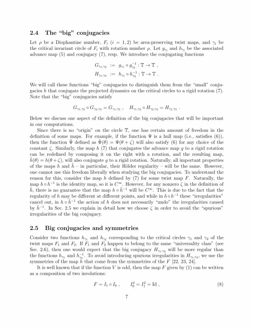
To use the CLP method, we need to apply repeatedly Fast Fourier Transform (FFT), whichis easiest to do if the values of the function K in (13) are known at 2N equally spaced pointsin the interval [0, 1) for some positive integer N . However, as we describe in Sec. 4, we donot have control over the set of points at which the values of K can be computed (where Kstands for any of the functions R, g, h, h−1, H , G). Hence, the first step in applying theCLP method would be the computation of the values of K on an evenly spaced grid. If weknow accurately the values of K at M points in [0, 1), we can expect that by using someinterpolation method, we will be able to obtain the approximate values of K on 2N ≈ Mequidistant points, {2−Nj}2N−1

j=0 . To compute the approximate values of K on the equidistantgrid, we used cubic spline interpolation. Using interpolation poses the question of whetherthe interpolated values represent faithfully the true values of K. Naturally, the answer tothis question is no, but practically if M is large enough, the interpolated values will bevery close to the true values, which will allow us to compute many Fourier coefficients of Kaccurately. The degree of “contamination” of the Fourier spectra due to the interpolationdepends on the uniformity of the distribution of the M points at which the values of K isknown accurately (see Remark 4.2).

To apply the CLP method numerically, we observe that the operator(

∂∂t

)ηe−t

√−∆ used

in Theorem 3.1 is diagonal in a Fourier series representation: if K(θ) =∑

k∈Z Kke−2πikθ,

then (∂

∂t

)η

e−t√−∆K(θ) =

∑

k∈Z(−2π|k|)η e−2πt|k| Kk e

−2πikθ . (14)

Having computed the values of the spline interpolant to the function K on an equally spacedgrid, applying (13) is easy. Namely, we fix some values of the parameters η and t, performFFT to find Kk and compute the Fourier coefficients of

(∂∂t

)ηe−t

√−∆K. Then we apply in-

verse FFT to find the values of(

∂∂t

)ηe−t

√−∆K at the equally spaced set of points {2−Nj}2N−1

j=0 ;among these values we find the one with maximum absolute value – this value we take for thenumerical value of the left-hand side of (13). For a fixed value of η, we repeat this procedurefor many values of t (we used several hundred values of t in our computations). Accordingto (13), if we plot

log

∥∥∥∥(∂

∂t

)η

e−t√−∆K

∥∥∥∥L∞(T)

versus log t , (15)

the points should lie below a straight line of slope κ− η. As pointed out in Remark 3.3 (seealso Remark 4.3) the points on the log-log plot should not only be below this straight line,but should close to it. We perform linear regression to find the slope of this line, from whichwe find κ.

12

4 Numerical results

4.1 Twist maps studied

We study numerically a set of one-parameter families of area-preserving twist maps of theform (1), each family having a different function V . Within each family we find numericallythe value Λ(σG) of the parameter λ for which the golden invariant circle is critical. The setof functions V (all of them odd) that we selected is the following:

1. The standard (Taylor-Chirikov) map:

V1(θ) = − 1

2πsin 2πθ . (16)

2. The “standard map with two harmonics”:

V2(θ) = − 1

2π[sin(2πθ)− 0.03 sin(6πθ)] . (17)

3. The “critical standard map with two harmonics”:

V3(θ) = − 1

2π

[sin(2πθ)− 1

2sin(6πθ)

]. (18)

For this choice of coefficients, the first three derivatives of V (θ) at θ = 0 are zero.

4. The “0.2-analytic map”:

V4(θ) = − 1

2π

sin(2πθ)

1− 0.2 cos(2πθ). (19)

This map has infinitely many nonzero Fourier coefficients. It would be very interestingto study this map when the coefficient of the cosine function in the denominator isclose to 1, but then it would be extremely difficult to compute periodic orbits.

5. The “0.4-analytic map”:

V5(θ) = − 1

2π

sin(2πθ)

1− 0.4 cos(2πθ). (20)

6. The “tent map”:

V6(θ) =

17∑

j=1

cj sin(2πjθ) , (21)

where cj = (−1)j+1

24

π2j2for j odd, and cj = 0 for j even, are the Fourier coefficients of

the function

V(θ) =

−4θ , for 0 ≤ θ < 14,

4θ − 2 , for 14≤ θ < 3

4,

4− 4θ , for 34≤ θ < 1 .

The function V6 is close to the piecewise linear continuous function V.

13

Our numerical experiments were performed with the twist maps coming from the abovesix functions V (θ) and the corresponding values Λ(σG), following the steps below.

1. As discussed in Sec. 3.1, the invariant circle of rotation number σG can be obtained asa limit of periodic orbits of rotation numbers equal to ratios of consecutive Fibonaccinumbers, ρm = Qm−1/Qm. We chose to compute hyperbolic periodic orbits, and foundthe values of Λ(σG) by applying Greene’s residue criterion.

2. The highest approximant to the critical invariant circle that we computed was a peri-odic orbit with rotation number Q29/Q30 = 832040/1346269. The value of Λ(σG) wasdetermined by using the condition that the difference, |R30 − R29| of the residues ofthe periodic orbits with periods Q29 and Q30 be zero (in practice, we wanted that thisdifference be smaller than 10−10). The periodic orbits were computed with an errornot exceeding 10−23.

3. We computed the hyperbolic periodic orbit {(θm, rm)}M−1m=0 of period M = Q30. The

values of the advance map g (5) at the points θm (m = 0, 1, . . . ,M − 1) were thencomputed by g(θm) = θm+1 (here and below, we take mod 1 wherever needed). Thevalues of the conjugacy h at the pointsmσG (which corresponds tom applications of therigid rotation by σG to 0) are given by h(mσG) = θm, and, similarly, h−1(θm) = mσG.

4. In our Fourier-analysis-based CLP method we need to deal with periodic functions, sowe compute the “periodized” versions, g − Id, h − Id, h−1 − Id, of the functions g, h,and h−1. Then we sort the periodized functions with respect to their argument; thefunction R is already periodic, so we just sort its values.

5. The periodic functions are passed to the cubic spline interpolation routine to findapproximations to the values of the corresponding functions on a uniformly spacedgrid of 2N points; we used N = 20.

6. The interpolated values of the functions are given to the CLP algorithm to computetheir Holder regularity. We used integer values of η in (13) from 1 to 5, and for eachanalyzed function chose the value of η that gave the best straight line on the log-logplot (15). The log-log plots for the other values of η were used as a consistency check.

Remark 4.1. In computing the big conjugacies Hγ1,γ2 , we had to take special care of thepreserving the symmetries of the maps h. For each critical circle we studied, we needed tofind the appropriate value of the constant ζ and shift the argument of the correspondingfunction h as explained in Sec. 2.5.

4.2 Critical invariant circles – visual explorations

In Fig. 1 we show the critical invariant circles which, by the definition (4), are graphs ofthe functions R corresponding to the six twist maps studied. The graphs of the “periodized

14

versions” of the advanced maps, g− Id, the conjugacies, h− Id, and their inverses, h−1− Id,are plotted in Figures 2, 3, and 4, resp.

Figure 5 illustrates the self-similar nature the functions h; needless to say, the insets aretrue zooms of parts of the graph of the function.

Fig. 6 shows the graphs of several periodized big conjugacies H − Id; it is obvious thatthese functions are smoother than the “small” conjugacies h.

4.3 Fourier spectra, CLP method

Fig. 7 depicts log10 of the modulus of the kth Fourier coefficient of a periodized conjugacy (h−Id) versus log10 k; here h is the conjugacy corresponding to the twist map F with V3 (18). Thehorizontal distance between two adjacent high peaks is approximately equal to | log10 σG| ≈0.209, which is a manifestation of the self-similarity at small scales. The log10-log10 plots ofthe Fourier spectra of the functions (g− Id) and (h−1− Id) for the same map F are given inFig. 8.

Remark 4.2. Note that the spectrum of h is very accurate even at length-scales ∼ 10−6,while the spectrum of h−1 is quite noisy. As explained in Sections 3.2.2 and 4.1, the mainreason for this is that the exact values of h are known at the points (mσG)mod 1, whichare almost uniformly distributed on T. On the other hand, we know the exact values ofof g and h−1 at the very nonuniformly distributed points of the form gm(θ0) (because theunderlying invariant measure is singular – see Sec. 5.2), which results in the presence of biggaps between these points and, hence, distorted values of the spline interpolant.

In Fig. 9 we show several plots of log10 of the left-hand side of (13) versus log10 t. The sixlines in each group of lines of similar slope correspond to the six different choices (16)–(21)of functions V , and the lines in each group come from the same value of η in (13). Eachon the “lines” in the figure in fact consists of 400 points (visually indistinguishable). Thecomputer time spent on the CLP analysis is of the order of one minute per point (we used220 Fourier coefficients to compute each of these points).

We computed the regularity by performing linear regression on the points on graphs likethe one in Fig. 9, in the regions where the points follow more or less a straight line. As onecan see from this figure, for t close to 1 (i.e., log10 t ≈ 0), the graphs for different functions arenot straight lines, then as t decreases they form more or less straight lines, and as t decreasesfurther, these lines level out. This behavior can be understood intuitively from (14) – fort ≈ 1 the high-k Fourier coefficients are strongly suppressed by the factor (−2π|k|)η e−2πt|k|,so the CLP method still does not “feel” the asymptotic self-similarity of the functions atsmall length-scales; in the other extreme, the leveling-out of the lines for very small t comesfrom the fact that in our computations we use a finite – albeit very large – number of Fouriercoefficients.

Remark 4.3. The “straight lines” in Fig. 9 are not really straight (which has been noticedin different contexts in [4, 24]). We show this effect in Fig. 10, which was created as follows.We took the six lines for η = 2 from Fig. 9, and for each of them we computed the slope

15

of the line as a function of the horizontal coordinate in the figure, log10 t. To compute thisslope, we took each pair of adjacent points on the line and found the slope of the straight lineconnecting these points. The distance between two consecutive peaks in Fig. 9 is | log10 σG|;more interestingly, as log10 t becomes more negative, the lines tend to the same wavy line,until all lines reach saturation around log10 t ≈ −4.5.

4.4 Global Holder regularities – numerical results

Table 1 summarizes our numerical results. The first column gives the map V used in thenumerical computations (for the six functions V given by (16)–(21)). In the other columnswe give the the values of the (global) Holder exponent κ of the function R (representingthe invariant circle as a graph in the (θ, r)-plane), the advance map g, the conjugacy h andits inverse, h−1, coming from the (dynamics on) the golden critical invariant circle of thecorresponding area-preserving twist map F . The notations used are the following: 1.85(15)stands for 1.85± 0.15, and 0.726(3) for 0.726± 0.003. Note that within the numerical error,κ(R) = κ(g), as expected.

We also computed the Holder regularities of all big conjugacies H between each of thesix functions h1, . . ., h6 (coming from V1, . . ., V6) with all other hj’s. We applied the CLPmethod to find that the regularity of all thirty functions H studied is

κ(H) = 1.80± 0.15 . (22)

5 Discussion and conclusion

In Sections 5.1 and 5.2 we point out some relationships between our results and previousstudies related to universal scaling factors and singular measures. In the final Section 5.3,we recapitulate our findings.

5.1 Holder regularity and scaling factors

Here we will explain how the scaling of the distances of closest returns of the iterates of apoint gives bounds on the Holder regularity of some of the functions we study. Our analysishere is reminiscent of the analysis in [4, Sec. 8.2].

We start by recalling the crucial observation of Kadanoff and Shenker [1, 2] (see also[15, Sec. 4.4]) of the existence of universal scalings in the distribution of the iterates of theTaylor-Chirikov map on the critical invariant circle γ in neighborhoods of certain pointsof γ. Let θrar ∈ T stand for the value around which the iterates of the function g are mostrarefied (in our notations θrar =

12, while in [2] θrar = 0). Let θden ∈ T stand for the value

around which the iterates of the function g are most dense (in our notations θrar = 0, whilein [2] it is θrar =

12). Since by Theorem 2.2 the function R is Lipschitz, around the points

(θrar, R(θrar)) and (θden, R(θden)), the iterates of any point on γ under F are most rarefied,resp. dense. Shenker and Kadanoff found that the critical invariant circle in a neighborhood

16

of θrar is asymptotically invariant under simultaneous scalings in both θ- and r-directions,with scaling factors

α0 ≈ −1.414836 (in θ) , β0 ≈ −3.0668882 (in r)

(see also the bounds on these values in Stirnemann [36]). This implies that, for large n,

gQn+1(θrar)− θrargQn(θrar)− θrar

≈ α−10 ,

R(gQn+1(θrar))− R(θrar)

R(gQn(θrar))−R(θrar)≈ β−1

0 . (23)

The scaling around θden is a bit more complicated – it is called “step-3” scaling for obviousreasons:

gQn+3(θden)− θdengQn(θden)− θden

≈ α−13 ,

R(gQn+3(θden))−R(θden)

R(gQn(θden))− R(θden)≈ β−1

3 , (24)

where the “step-3” scaling factors are

α3 ≈ −4.84581 (in θ) , β3 ≈ −16.8597 (in r) .

To understand heuristically why these scalings give restrictions on the Holder regularityof R, set ∆θ := gQn+1(θrar) − θrar, ∆r := R(gQn+1(θrar))− R(θrar) for some large value of n.Then if the local Holder exponent of R at θ = θrar is κ, we will have |∆r| ∼ |∆θ|κ. Ifthe graph of R is asymptotically invariant around (θrar, R(θrar)) with respect to the scalings(23), we will have |β0∆r| ∼ |α0∆θ|κ. “Dividing out” the last two relationships, we obtain

|β0| ∼ |α0|κ, i.e., κ ∼ log |β0|log |α0| . This argument (which can easily be made rigorous) implies

that the (global) Holder exponent of R does not exceed log |β0|log |α0| ≈ 3.22945. The scaling (24)

yields a tighter bound on the Holder regularity of R:

κ(R) ≤ log |β3|log |α3|

≈ 1.7901 . (25)

Note that the fact that the scaling (24) is “step-3” (as opposed to “step-1”) is irrelevant forthe bounds on the Holder regularity.

To obtain bounds on κ(h) and κ(h−1), we use Lemma 8.1 from [4], which says that if thefunction h conjugates f1 and f2, h ◦ f1 = f2 ◦ h, and if for some sequence of positive integersQn the functions fj (j = 1, 2) behave in a neighborhood of the fixed point θfix = h(θfix) of has follows:

fQn

j (θfix) = θfix + Cjη−nj + o(η−n

j )

for some constants ηj and Cj, then κ(h) ≤ log |η2|log |η1| . Applying this to the definition of h and

using the well-known fact that (Qn σG)mod 1 ≤ CσnG, we obtain the bounds

κ(h) ≤ log |α−10 |

log |σG|≈ 0.721125 , κ(h−1) ≤ log |σ3

G|log |α−1

3 | ≈ 0.91478 . (26)

A comparison with Table 1 suggests that these bounds are saturated.

17

5.2 Conjugacies and singular measures

The functions whose Holder regularity we study are defined through high iterates of maps.For example, the graph of the function R defined by (4) is nothing but the the critical invari-ant circle γ of F which is is filled densely by the iterates F n(θ0, r0) of some point (θ0, r0) ∈ γ.Here we discuss how some characterizations of the singularities in the distribution of theiterates of F on γ are related to the Holder regularity of some of the functions considered.

Hentschel and Procaccia [37] pointed out the importance of the generalized (Renyi) di-mensions D(q) of a singular measure for dynamical systems; these quantities have beendefined previously in the context of probability theory by Renyi [38]. Halsey et al in theirseminal paper [3] related heuristically the Renyi dimension of a singular measure to thespectrum of singularities f(α). We recall that f(α) is the Hausdorff dimension of the set Eα

of points where the measure has singularity of strength α. The spectrum f(α) is a functionsupported on the interval [αmin, αmax], where αmin = D(∞), resp. αmax = D(−∞), describethe scaling behavior of the measure in the region where the measure is most dense, resp.most rarefied.

Let (θ0, r0) be an arbitrary point on the critical invariant circle γ of the area-preservingtwist map F . Then the distribution of the iterates in a very long orbit, {F n(θ0, r0)}Kn=0,approaches as K → ∞ the “density” of the measure on γ that is invariant with respectof the restriction of the map F onto γ. (We put “density” is quotation marks because forsingular measures this is not a function, but a set of Dirac δ-distributions.) This invariantmeasure on γ induces an invariant measure µg of the map g on T. It is easy to see that (7)implies that

h−1(θ) =

∫ θ

0

dµg

(for an appropriately chosen ζ in the redefinition of h as in Sec. 2.5). This relationshipimplies that the spectrum of singularities f(α) of the measure µg is the same as the Holderspectrum fH(α) of the function h−1. By definition, fH(α) is the Hausdorff dimension of theset where the local Holder exponent of the function is equal to α; for a readable account werefer the reader to Jaffard [39]. The (global) Holder regularity κ(φ) of a function φ is equalto the lowest end, αmin, of the support of the Holder spectrum, fH(α), of φ.

Osbaldestin and Sarkis [40] applied the method of [3] to determine numerically the func-tions f(α) and D(q) of the invariant measure µg coming from the distribution of iterates ofthe Taylor-Chirikov map F on the golden invariant circle. They found that

αmin = D(∞) ≈ 0.915 , αmax = D(−∞) ≈ 1.387 ≈ 1

0.720.

Comparing with the values in Table 1, the reader should recognize that their αmin is nothingbut our κ(h−1), while αmin is equal to the inverse of the regularity of the conjugacy h.

Buric et al [41, 42] studied numerically the Taylor-Chirikov map and the map (1) withV (θ) = 1

2sin 2πθ+ 1

4sin 4πθ, for rotation numbers with continued fraction expansions of the

form [S, 1∞] := [S, 1, 1, 1, . . .], [S, 2∞], [S, 3∞], [S, 4∞], where S stands for some short stringof positive integers. They found that f(α) and D(q) depend only on the tail but do not

18

depend on the initial part S as well as on whether the Taylor-Chirikov map or the othermap was used in their numerics.

Other papers related to numerical computations of singular measures on critical invariantcircles of area-preserving twist maps are Shi and Hu [43, 44], where the methods of [3] wereused, and Hunt et al [45], where the authors used the thermodynamic formalism developedin [46] to compute the information dimension D(1) of the standard map for different rotationnumbers.

5.3 Conclusion

We computed accurately the golden critical invariant circles for six twist maps of the form (1)and the global Holder regularity κ of some functions related to the dynamics on these circles.Our numerical experiments lend credibility to Conjectures 2.3, 2.4 and 2.5 concerning theuniversality of the regularities of the functions R, g, h, h−1 and H (see Table 1 and (22)).Yamaguchi and Tanikawa [47] found numerically that the golden invariant circle (given by thefunction R) of the Taylor-Chirikov map is differentiable but R′ is not of bounded variation;our studies significantly narrow the numerical bounds on κ(R) for this and for other maps.

Our results seem to indicate that the regularities of R, h, and h−1 saturate the upperbounds (25) and (26) coming from previous studies of scaling exponents.

Our finding that κ(H) is greater than κ(h) and κ(h−1) by a comfortable margin (cf. Con-jecture 2.6) has an interesting consequence. As discussed in Sec. 5.2, the Holder regularityof h and h−1 is different at different points, and for each α ∈ (αmin, αmax), the set Eα (wherethe pointwise Holder exponent of h−1 is α) has Hausdorff dimension fH(α) strictly between0 and 1. Previous numerical studies indicated that fH(α) are the same for different maps F .Our finding shows that the “irregularities” of functions h coming from different maps F areinterspersed in the same way in [0, 1] for all twist maps studied. Note that this does notmean that for a certain value of α the sets Eα are the same for different F in the sameuniversality class – only the way all sets Eα for different α are interwoven is universal.

It would be interesting to apply wavelet-maxima methods for pointwise regularity [48, 49](see also the rigorous analysis in [39]) to the problem studied in this paper and to comparethe results of the wavelet analysis with the results about the singular invariant measures.

As a by-product of our studies, we have computed millions of Fourier coefficients of thefunctions h, and noticed some self-similarity properties that to the best of our knowledgehave not been observed before. Presently we are working on understanding these properties.

19

Acknowledgments

We would like to express our gratitude to Rafael de la Llave, who introduced the authorsof the present paper to each other, suggested the problem, and took an active part in theearly stages of this research. We have profited immensely from his expert advice and friendlyprodding throughout our work on the paper.

The research of NP was partially supported by National Science Foundation grant DMS-0405903 and by the Michigan Center for Theoretical Physics (where part of this researchwas conducted). The authors would like to thank IIMAS-UNAM for supporting NP’s visitsto Mexico City.

Our computations were carried out on the computers of IIMAS-UNAM and the Depart-ment of Mathematics of the University of Texas. AO would like to thank Ana Perez forthe computational support. We used the doubledouble software developed by Keith Briggs,and the convenient plotting tool Grace [50] (a descendant of ACE/gr developed by Paul J.Turner). We express our thanks to all these people and organizations.

20

References

[1] L. Kadanoff, “Scaling for a critical Kolmogorov-Arnold-Moser trajectory”, Phys. Rev.Lett. 47 (1981), 1641–1643.

[2] S. Shenker and L.P. Kadanoff, “Critical behavior on a KAM surface: I. Empiricalresults”, J. Stat. Phys. 27 (1982), 631–656.

[3] T. C. Halsey, M. H. Jensen, L. P. Kadanoff, I. Procaccia, B. I. Shraiman, “Fractalmeasures and their singularities: The characterization of strange sets”, Phys. Rev. A33 (1986), 1141–1151, reprinted in [51, pp. 540–550].

[4] R. de la Llave and N. Petrov, “Regularity of conjugacies between critical circles maps:An experimental study”, Experiment. Math. 11 (2002), 219–241.

[5] C. Tresser and P. Coullet, “Iterations d’endomorphismes et groupe de renormalisation”,C. R. Acad. Sci. Paris Ser. A-B 287 (1978), A577–A580.

[6] M. J. Feigenbaum, “Quantitative universality for a class of nonlinear transformations”,J. Stat. Phys. 19 (1978), 25–52.

[7] M. J. Feigenbaum, “The universal metric properties of nonlinear transformations”, J.Stat. Phys. 21 (1979), 669–706, reprinted in [51, pp. 207–244].

[8] S. Shenker, “Scaling behavior in a map of a circle onto itself: empirical results”, Phys.D 5 (1982), 405–411, reprinted in [51, pp. 405–411].

[9] P. Collet, J. P. Eckmann and O. E. Lanford, III, “Universal properties of maps on aninterval”, Comm. Math. Phys. 76 (1981), 211–254.

[10] M. J. Feigenbaum, L. P. Kadanoff, and S. J. Shenker, “Quasiperiodicity in dissipativesystems: a renormalization group analysis”, Phys. D 5 (1982), 370–386.

[11] S. Ostlund, D. Rand, J. Sethna, and E. Siggia, “Universal properties of the transitionfrom quasiperiodicity to chaos in dissipative systems”, Phys. D 8 (1983), 303–342.

[12] R. S. MacKay, “A renormalisation approach to invariant circles in area preserving twistmaps”, Phys. D 7 (1983), 283–300, reprinted in [53, pp. 462–479].

[13] J. D. Meiss, “Symplectic maps, variational principles, and transport”, Rev. ModernPhys. 64 (1992), 795–848.

[14] C. Gole, Symplectic Twist Maps, World Scientific, 2001.

[15] R. S. MacKay, “Renormalization in Area Preserving Maps”, PhD Thesis, PrincetonUniversity, 1982; published with notes as R. S. MacKay, Renormalization in Area-Preserving Maps, World Scientific, Singapore, 1993.

21

[16] G. D. Birkhoff, “Surface transformations and their dynamical applications”, Acta Math.43 (1920), 1–119, reprinted in [52, pp. 111–229].

[17] J. Mather, “Nonexistence of invariant circles”, Ergodic Theory Dynam. Systems 4(1984), 301-309, reprinted in [53, pp. 395–403].

[18] J. J. Mather and G. Forni, “Action minimizing orbits in Hamiltonian systems”, Tran-sition to Chaos in Classical and Quantum Mechanics (Montecatini Terme, 1991), J.Bellissard et al, Eds., Springer, Berlin, (1994), 92–186.

[19] A. Ya. Khinchin, Continued Fractions, Dover, Mineola, NY, 1997.

[20] R. S. MacKay and I. C. Percival, “Converse KAM: theory and practice”, Comm. Math.Phys. 98 (1985), 469–512.

[21] I. Jungreis, “A method for proving that monotone twist maps have no invariant circles”,Ergodic Theory Dynam. Systems 11 (1991), 79–84.

[22] R. DeVogelaere, “On the structure of symmetric periodic solutions of conservative sys-tems, with applications”, In Contributions to the Theory of Nonlinear Oscillations, S.Lefschetz (Ed.), Princeton University Press, 1958, pp. 53–84.

[23] J. M. Greene, “A method for determining a stochastic transition”, J. Math. Phys. 20(1979), 1183–1201, reprinted in [53, pp. 419–437].

[24] A. Apte, R. de la Llave and N. P. Petrov, “Regularity of critical invariant circles of thestandard nontwist map”, Nonlinearity 18 (2005), 1173–1187.

[25] J. A. Ketoja, “Renormalisation in a circle map with two inflection points”, Phys. D 55(1992), 45–68.

[26] J. A. Ketoja and R. S. MacKay, “Rotationally-ordered periodic orbits for multiharmonicarea-preserving twist maps”, Phys. D 73 (1994), 388–398.

[27] C. Falcolini and R. de la Llave, “Numerical calculation of domains of analyticity per-turbation theories in the presence of small divisors”, J. Stat. Phys. 67 (1992), 645–666.

[28] R. de la Llave and A. Olvera, “The obstruction criterion for non-existence of invariantcircles and renormalization”, Nonlinearity 19 (2006) 1907–1937.

[29] R. de la Llave and R. P. Schafer, “Rigidity properties of one dimensional expandingmaps and applications to renormalization”, Manuscript, 1996.

[30] G. D. Birkhoff, “An extension of Poincare’s last geometric theorem”, Acta Math. 47(1925), 297–311, reprinted in [52, pp. 252–266].

[31] A. Katok and B. Hasselblatt, Introduction to the Modern Theory of Dynamical Systems,Cambridge University Press, Cambridge, 1995.

22

[32] A. Olvera and C. Simo, “An obstruction method for the destruction of invariant curves”,Phys. D 26 (1987), 181–192.

[33] C. Falcolini and R. de la Llave, “A rigorous partial justification of Greene’s criterion”,J. Stat. Phys. 67 (1992), 609–643.

[34] T. Carletti, “The 1/2-complex Bruno function and the Yoccoz function: a numericalstudy of the Marmi-Moussa-Yoccoz conjecture”, Experiment. Math. 12 (2003), 491–506.

[35] E. Stein, Singular Integrals and Differentiability Properties of Functions, Princeton Uni-versity Press, Princeton, 1970.

[36] A. Stirnemann, “Towards an existence proof of MacKay’s fixed point”, Commun. Math.Phys. 188 (1997), 723–735.

[37] H. G. E. Hentschel and I. Procaccia, “The infinite number of generalized dimensions offractals and strange attractors”, Phys. D 8 (1983), 435–444.

[38] A. Renyi, “On measures of entropy and information”, in Proceedings of the FourthBerkeley Symposium on Mathematical Statistics and Probability, University of Cali-fornia, June 20–July 30, 1960, Vol I, University of California Press, Berkeley, 1961,pp. 547–561.

[39] S. Jaffard, “Multifractal formalism for functions. I. Results valid for all functions. II.Self-similar functions”, SIAM J. Math. Anal. 28 (1997), 944–970, 971–998.

[40] A. H. Osbaldestin and M. Y. Sarkis, “Singularity spectrum of a critical KAM torus”,J. Phys. A 20 (1987), L953–L958.

[41] N. Buric, M. Mudrinic and K. Todorovic, “Equivalent classes of critical circles”, J. Phys.A 30 (1997), L161–L165.

[42] N. Buric, M. Mudrinic and K. Todorovic, “Universal scaling of critical quasiperiodicorbits in a class of twist maps”, J. Phys. A 39 (1998), 7848–7854.

[43] J. Shi and B. Hu, “Crossover phenomena in the multifractal behavior of invariant cir-cles”, Phys. Lett. A 156 (1991), 267–271.

[44] B. Hu and J. Shi, “Nonanalytic twist maps and Frenkel-Kontorova model”, Phys. D 71(1994), 23–38.

[45] B. R. Hunt, K. M. Khanin, Ya. G. Sinai, and J. A. Yorke, “Fractal properties of criticalinvariant curves”, J. Stat. Phys. 85 (1996), 261–276.

[46] E. B. Vul, Ya. G. Sinai, and K. M. Khanin, “Feigenbaum universality and thermo-dynamic formalism”, Russian Math. Surveys 39 (1984), 1–40, reprinted in [51, pp.491–530].

23

[47] Y. Yamaguchi and K. Tanikawa, “A remark on the smoothness of critical KAM curvesin the standard mapping”, Prog. Theor. Phys. 101 (1999), 1–24.

[48] A. Arneodo, E. Bacry and J. F. Muzy, “The thermodynamics of fractals revisited withwavelets”, Phys. A 213 (1995), 232–275.

[49] J. F. Muzy, E. Bacry and A. Arneodo, “The multifractal formalism revisited withwavelets”, Internat. J. Bifur. Chaos Appl. Sci. Engrg. 4 (1994), 245–302.

[50] The Grace team, Grace homepage. http://plasma-gate.weizmann.ac.il/Grace/.

[51] P. Cvitanovic, Universality in Chaos, IOP Publishing, Bristol, 1989.

[52] G. D. Birkhoff, Collected Works, Vol II, Dover, New York, 1968.

[53] R. S. MacKay and J. D. Meiss, Hamiltonian Dynamical Systems, Adam Hilger, Bristol,1993.

24

Tables

F with: κ(R) κ(g) κ(h) κ(h−1)

V1 1.83(9) 1.83(9) 0.722(1) 0.92(1)V2 1.79(6) 1.75(9) 0.721(1) 0.92(1)V3 1.83(4) 1.84(3) 0.724(2) 0.93(2)V4 1.86(8) 1.86(8) 0.722(1) 0.92(1)V5 1.85(5) 1.85(5) 0.724(2) 0.93(1)V6 1.85(15) 1.88(12) 0.726(3) 0.93(2)

Table 1: Regularities of the functions R, g, h, and h−1 for the golden critical invariant circlesof different maps F .

25

Figure captions

Caption to Figure 1:

Critical invariant circles, r = R(θ), of the maps corresponding to the maps V1, V2, . . .,V6 given by (16)–(21) (V1 = thin solid line, V2 = thick solid line, V3 = dotted line, V4= thin dashed line, V5 = thick dashed line, V6 = dot-dashed line).

Caption to Figure 2:

”Periodized” advance maps g − Id (notation same as in Fig. 1).

Caption to Figure 3:

“Periodized” conjugacies h− Id (notation same as in Fig. 1).

Caption to Figure 4:

“Periodized” inverse conjugacies h−1 − Id (notation same as in Fig. 1).

Caption to Figure 5:

Zooming in the graph of the function h− Id corresponding to the map V2 (17).

Caption to Figure 6:

“Periodized” big conjugacies H − Id.

Caption to Figure 7:

Plot of log10

∣∣∣(h− Id

)

k

∣∣∣ versus log10 k, where h corresponds to the map F coming form

the function V3 (18).

Caption to Figure 8:

Plot of log10

∣∣∣(g − Id

)k

∣∣∣ and log10

∣∣∣(

h−1 − Id)k

∣∣∣ versus log10 k, for the same map F as

in Fig. 7. The impulses correspond to (g − Id), and the dots above them to (h−1 − Id).

Caption to Figure 9:

Plots of log10

∥∥∥(

∂∂t

)ηe−t

√−∆K

∥∥∥L∞(T)

versus log10 t for the functions K = (h − Id) for

the twist maps coming from V1, . . ., V6, for η = 2 (shallowest lines), η = 3, and η = 4(steepest lines).

Caption to Figure 10:

Slope of the lines on Fig. 9 as a function of log10 t (see the text). The notation is thesame as in Fig. 1.

26

Figures

0 0.2 0.4 0.6 0.8 1θ

0.4

0.5

0.6

0.7

0.8

r

Figure 1:

27

0 0.2 0.4 0.6 0.8 1θ

0.4

0.5

0.6

0.7

0.8

Figure 2:

28

0 0.2 0.4 0.6 0.8 1θ

-0.1

-0.05

0

0.05

0.1

Figure 3:

29

0 0.2 0.4 0.6 0.8 1θ

-0.1

-0.05

0

0.05

0.1

Figure 4:

30

0 0.2 0.4 0.6 0.8 1θ

0.46

0.48

0.5

0.52

0.54

Figure 5:

31

0 0.2 0.4 0.6 0.8 1θ

-0.06

-0.04

-0.02

0

0.02

0.04

0.06

Figure 6:

32

Figure 7:

33

Figure 8:

34

-5 -4 -3 -2 -1 0

0

2

4

6

8

10

Figure 9:

35

-5 -4 -3 -2 -1 0

-1.4

-1.35

-1.3

-1.25

-1.2

-1.15

Figure 10:

36