Embed Size (px)
Citation preview
Regulating Local Public Utilities byProfit-Sharing∗
Michele Moretto and Paola Valbonesi†
October 2001
AbstractThis paper concerns “profit-sharing” within an incomplete regu-
latory contract where a municipality delegates a risk-neutral firm tomanage a local utility. Together with a price cap regulation (PCR)mechanism, the contract envisages the possibility of the municipalityrevoking the contract if the firm’s profits are percieved “excessively”high. We show that when this threat is credible and the cost of exer-cising it is not too high, a long-term efficient equilibrium arises whichguarantees the firm with an appropriate level of profits. The con-sequent regulation timing consists of an endogenous regulatory lagwhere the regulation has a PCR nature, followed by a period of RORin which the firm is motivated to adjust its price downward to avoidcontract recall. We also show that excessive revocation costs make thefirm an unregulated monopolist with an infinite regulatory lag whereROR looks like a pure PCR.Key words: Public utilities, Regulatory contracts, Profit-
sharing, Stochastic games.JEL: C73, L33, L51
∗This study is part of a research project financed by the Italian Ministry of Universityand Research (MURST 40%; 1999-2000) and the University of Padova (Progetto Ateneo2000). An earlier version of this paper appeared in the Fondazione ENI, Nota di lavoroFEEM, no.51/2000. We benefitted from discussion with Cesare Dosi, Gerard Mondelloand seminar participants at Universities of Bologna and Padova, and EARIE Conference2000, Losanna. The authors alone are responsible for any remaining errors.
†Department of Economics, University of Padova, Via del Santo 33, Italy, E-mail:[email protected] ; [email protected]
1
1 IntroductionThis paper investigates “profit-sharing” device in a regulatory contract signedbetween a municipality and a private firm for the supply of local public utilityservices. The type of administrative contract we study envisages for themunicipality the temporary delegation of the utility provision to a privateoperator. While the ownership of the asset is maintained public, “the right touse it” becomes private. This form of delegation is justified by the presenceof a residual segment of public utility industries which - notwithstandingtechnological change - is still a natural monopoly and is likely to remain soin the foreseeable future. The entire traditional business of a firm in a utilityindustry is no longer defined as a natural monopoly; however, in services suchas sewage and fresh water, urban waste and provision of public transport,the problem of access facilities remains and - consequently - the problem ofnatural monopoly regulation with these residual segments. Here, therefore,delegation of the contract to a private firm becomes an alternative to directpublic management or to full privatization of the asset.Both the municipality and the private firm have potential gains from this
delegation contract: on the one side, the private firm has returns guaranteedby the contract exclusivity and, on the other side, the municipality promotesefficiency and better and/or cheaper service injecting - through the privatefirm provision - technological, financial and managerial resources into theutility supply. The clean-cut allocation of functions between the municipalityand the private firm - on the one hand planning, control and regulation ofthe utility and on the other hand management of the utility - is defined andruled in the contract: in this perspective, the contract is itself a regulatorymechanism where the municipality has the position of residual decision makerwith respect to the private firm as a consequence of property rights which itmaintains1.In local public utility services, the contract is usually delegated under spe-
cific institutional features differently qualified at national level: in France,the country with the longest experience in this field, the gestion déléguée inpublic utility sectors allows for various forms of contracts2 which are differ-
1The municipality’s role of residual decision maker can also be related to the need toprotect the customers’ “right to be served”. See about Goldberg (1976).
2Among these forms concession, affermage, régie intéressée, gérence are the mostknown and particularly used in the water sector (see about Carles and Dupuis, 1989;Lorraine, 1995).
2
ently characterized by the degree of delegation and by financial constraintson investments. Similarly, in Italy the concessione allows for two forms ofcontract3 on the grounds of the relative weight given to planned new invest-ment and to management of the utility itself. In Germany the industrialactivities of local public utility (Daseinsvorgsorgee) are delegated throughdifferent forms of contracts which have to take account for the Lander’s spe-cific legislation in these sectors4.Notwithstanding their different designs, all these contracts have common
features like the definition of a price regulation mechanism, an investmentplan and quality objectives in the service provision. Moreover, at juridicallevel, all these contracts share a dual nature: the administrative (public)nature on the basis of which the municipality holds a favourable positionwithin the contract, and the private nature via which the wishes of bothparties are expressed and the agreement is determined. In other words,they are incomplete regulatory contracts where the municipality plays therole of residual claimer in the relationship with the firm whenever futurecontingencies unspecified in the contract occur.Our analysis takes its cue from the evidence of these different positions
of the two parts in the contract. In particular, we focus on the point thatthe municipality is able to exercise the role of residual claimer revoking thecontract to the private firm: once the revocation applies, the managementof the utility is back in the hands of the municipality which can choose fromdirect management, or privatization of the asset, or delegation of the contractto another private firm.In the real world, revocation usually refers to the right of the municipality
to remove the delegation of the utility provision a) in the event of breach ofthe contract by the private operator (i.e. it may occur when the firm doesnot respect the terms established in the contract) and b) in the case of re-demption of the contract by the municipality itself (i.e. it may occur whenpolitical pressure - safeguarding collective welfare - induces the municipalityto consider the firm’s profits as “excessively” high). However, in these two
3These forms are called concessione di costruzione e gestione and concessione dierogazione di servizio: in the former new investment required by contract is primary withrespect to the management of the utility, while in the latter management of the utility isthe primary aim of the contract itself (see about Mameli, 1998).
4The most used forms of delegation contract in Germany are: Verwaltungshelfer, Of-fentliche Eirichtung in privater Regie, Nutzungsubertragung, Betreiber (see about Marcou,1995).
3
dimensions the municipality’s right to revoke has substantially different ori-gins: while in the former it relates to conditions made clear in the contract,in the latter it belongs to the different positions of the two parties in thecontract. In both the dimensions, the right of revocation is ruled in specificclauses of the contract where the timing, procedures and possible contractualindemnities belonging to the exercise of this municipality’s right are defined5.Though in the regulation of firms managing public utility there is a well-
developed literature concerning the use and effects of revocation when breachof contract occurs 6, no in-depth analysis has been performed when revocationoccurs via exercise by the municipality of its right to redeem the contract.We move from this lack in literature, and investigates revocation when theright of redemption hold7: in particular, we consider how the threat of themunicipality’s revocation affects the private firm’s decisions regarding devel-opment of its profits. We do this in a simple model where a risk-neutralfirm has been delegated to manage an indivisible public project whose prof-its evolve stochastically over time. Moreover, by the above discussion, weassume that the municipality has the right, at any time, to revoke delegationand return to direct management if the project is a positive net present valueinvestment. In this respect, therefore, revocation is analogous to a contrac-tual claim that displays option-like characteristics where the municipalityhas the right - but not the obligation - to purchase an asset (the utility) ofuncertain value for a present exercise price, and the value of such a claim isderived from the market value of the project. The exercise price refers to thesum necessary to overcome the obstacles to renewing direct management of
5It is interesting to stress here that while in Italy and in France these contracts aregoverned by administrative law, in Great Britain there is no law of public contract and thedelegation of public utilities’ provision to private operators (i.e. contracting out) is first andforemost a political choice that requires the issue of an ad hoc law for its implementation.Moreover, in Great Britain contracts between public authorities and private operators aresubject to private law: this means that relations between public authorities and privatefirms, and between private firms and users of the service, are outlined only within thecontract itself.The model developed here - as will be seen in the following sections - can also be
extended to contracting out where, within the contract of delegation to the private firm,there are explicit redemption clauses that reflect those considered in this analysis.
6Many contributions on this topic belong to the analogy between a regulatory contractand a law contract in determining appropriated damages to be paid in the event of breachby one of the parties (see about Lyon and Huang, 2000; Brennan and Boyd, 1997; Gregoryand Spulber, 1997; Lyon, 1995; Miceli and Segerson, 1994).
7Then, in the remainder of the paper revocation and redemption are used as synonyms.
4
the service such as contractual indemnities on the value of the investment,technological costs, recruiting and training costs as well as litigation costs ifthe firm decides to sue the municipality for recalling the contract. The optionwill be exercised optimally when the value of the project exceeds a triggervalue (i.e. an “allowed” level of profits) which is determined endogenously inthe model although the optimal exercise time remains stochastic8.We offer an optimal regulatory mechanism where the commitment by
the municipality to end the contract if the firm’s “allowed” level of profitsis exceeded ensures that the private operator will behave consistently withthe contract itself: once the firm’s costs or production conditions improve,it adjusts prices to keep its profits below the allowed level and therefore toprevent revocation. However, as the revocation threat is costly, a stochasticregulatory lag may follow during which prices are not revised and it is notoptimal for the municipality to recall the contract.We then look at the revocation from the perspective of collective welfare
maximization and discuss the specific characteristics of the dynamic regula-tory rule stemming from the continuous rate of hearing between the regulatedfirm and the municipality, as a tool for obtaining a long-term efficient equi-librium.Our model is closest in spirit to the theory of monopoly regulation in a dy-
namic setting, in which mechanisms such as rate-of-return regulation (ROR)and price-cap-regulation (PCR) arise endogenously as a self-enforcing andmutually beneficial equilibrium9. However, in this literature both the “regu-lator” and the “regulated” firm share the same bargaining power (i.e. bothplayers have the incentive to breach the contract) and they are not affectedby regulatory lags. Although playing a crucial role in determining the incen-tive property of the regulation mechanism, these lags are of fixed time andexogenous whereas in our setup, the different bargaining positions of the twoparties coupled with the municipality’s option to revoke determine these lagsendogenously as it is in the essence of ROR regulation (Laffont and Tirole,
8Brennan and Schwartz (1982) and Teisberg (1994) model the regulator’s future optionsto cut high profits (with possibility of expropriation) as a perpetual call option whichreduces the value of the regulated firm. Recently, referring to the French municipalities’negotiating disadvantage in the face of a cartelized water management, Clark and Mondello(2000) model the municipality’s right to revoke delegation as a perpetual call option.However, these models do not investigate optimal regulatory policy within the regulationprocess.
9See for example Salant and Woroch (1991, 1992) and Gilbert and Newbery (1989).
5
1994, p.15). Price reviews are initiated by the municipality when revocationis worth exercising. This excludes that price renewals being perceived as thetime in which the PCR takes some of the well-recognized inefficiencies ofROR. Only excessive revocation costs make the firm an unregulated monop-olist, where ROR resembles a PCR with an infinite regulatory lag (Crew andKleindorfer, 1996, p. 213). Furthermore, the result of an endogenous regu-latory lag may also explain the empirical evidence indicating that, althoughcontracts between local authorities and private operators are of limited du-ration, their renewals are often signed without any variations of contractualterms (Joskow and Schmalensee, 1986, p.7).On a formal level, our paper builds upon two distinct streams of literature.
The first one relates to the stochastic control techniques recently developedto identify optimal timing rules and optimal barrier regulations10. Thesetechniques have been widely used in the literature of irreversible investments(Pindyck, 1991; Dixit, 1992; Dixit and Pindyck, 1994), and emphasize therole of the option value of delaying investment decision, i.e. the value ofwaiting for better (although never complete) information on the stochasticevolution of a basic asset. The second one considers the existence of efficientsub-game perfect equilibria for infinite-horizon-threat-games where, in theabsence of a binding commitment for the threatener, it is an equilibrium forthe victim to make a stream of payment over time (Klein and O’Flaherty,1993; Shavell and Spier, 1996). The expectation of future payment keeps thethreatener from exercising its threat. Indeed, we formulate a time-dependentgame in continuous time, where optimal revocation for the municipality re-quires identification of the time at which to pay a sunk cost in return for apublic project whose value is stochastic. The municipality does not revokethe contract until revenues that it expects to earn from managing the invest-ment by itself is equal to the expected present value of the profits regulationthat the firm adopts11.The plan of the paper is as follows: Section 2 describes the model focusing
firstly on the contract and the timing, then on the firm’s value and finally onthe municipality’s option to revoke. Section 3 examines the regulation thatbelongs to this scheme. Section 4 discusses results and the policy implica-tions. Finally, the Appendix gives precise statements of the results derived10We refer here to the works of Harrison and Taksar (1983) and Harrison (1985).11See Moretto and Rossini (1997, 2001) for the formulation and application of these
infinite-horizon-threat-games.
6
heuristically in Section 3 with all the proofs.
2 The Basic Framework
We begin with a description of the key features of the regulatory contract,then we turn to the performance of the regulatory mechanism and to thepolicy implications.
2.1 The regulatory contract and its timinig
We consider a simple model where a self-interested-risk-neutral municipalitydelegates a risk-neutral firm to manage a one-time sunk indivisible publicproject. Here, what is called “delegation” is the temporary (although longduration) supply of a local public service by a municipality to some pri-vate operator under contractual relationship12. For the simple contract weconsider, the municipality maintains the ownership of the asset while thefirm has the “right to use it” and we assume that no new investments areundertaken during the delegation13. At t = 0, the parties sign a contractspecifying a price cap that consumers should pay for the service inclusiveof an automatic adjustment clause such as pt = pe(RPI−x)t, where the priceis allowed to increase by the difference between the expected inflation rate(the Retail Price Index, RPI) and an exogenously given expected increasein the productivity the firm should obtain over time (x). Moreover, the dele-gation contract also includes a revocation (redemption) clause by which themunicipality always has the right to recall delegation if the firm’s profits areperceived as “excessively” high, in favor of direct management of the util-ity14. However, to manage the utility the municipality has to pay a (sunk)12In principle, our analysis could be applied to utilities of global range (national utili-
ties), but given our assumption on revocation of the contract, the local dimension is morerealistic. In fact, the management of a contract at national level can affect the delegatedfirm’s bargaining power which, in turn, can affect the revocation decision (regulatory cap-ture).13For the analysis of a regulatory contract where new investments are negotiated be-
tween a municipality and a private firm see Dosi, Moretto and Valbonesi (2001).14In our framework, the private operator will never refuse to operate because the utility
is always a positive net present value project, as described below.
7
revocation cost I which, without any loss of generality, we assume does notinclude any contractual indemnities on the value of the asset.The setting of the game is the following. At time zero, the municipality
assigns the contract to the firm and negotiates the price celing p and thex factor. On the basis of the estimated revocation cost I and the expectedevolution of the firm’s profits, the municipality determines an upper triggerlevel of profits15. The firm is allowed to continue unaltered until this level iscrossed. The first time the municipality ascertains that this trigger value hasbeen crossed, it intervenes calling for a revocation of the contract. The firmreacts to the commitment of the municipality to end the contract by adjustingits price downward to keep its profits below the allowed level. Once reduced,the new price remains valid until profits cross the trigger level again, inducinga new price revision. The firm can choose to reduce its profits to guaranteethe continuity of delegation or to deviate and keeps its profits, knowing thatconsequently the contract will end.This simple setting captures the characterisitcs of a delegation contract
where the PCR is negotiated under the threat of a more stringent renegotia-tion and where the renegotiation timing is determined endogenously by thedynamic of the contract, i.e. the PCR incorporates an endogenous “profit-sharing” mechanism.
2.2 The firm’s value
Once set up, we assume that the single project allows some flexibility in itsoperation at each time t ≥ 0, by varying certain inputs according to thefollowing production function:
qt = atlϕt with 0 < ϕ < 1 (1)
where qt denotes the production at time t, lt is the operating input such aslabor (or some intermediate input) and at is a technology-efficiency parameterwhose value is determined stochastically. The operating input is a perfectlyflexible factor which can be rented at the instantaneous price wt whose value15Asymmetric information at time zero between the firm and the municipality about
the revocation cost does not preclude the timing of the game.
8
is also stochastic. The operating cash flow function is defined as:16
π(pt, at, wt) = maxltptqt − wtlt (2)
subject to equation (1)and the price-cap pt ≤ pt ≡ pe(RPI−x)t. For sake ofsimplicity and without sacrificing in generality, we assume that in the abovemaximization the price constraint is always binding, which allows us to writethe operating cash flow as:17
π(pt, θt) = Π(pt)θt (3)
where:Π(pt) = (1− ϕ)ϕ1−ξ pξt
and:θt = θ(at, wt) ≡ aξtw1−ξt with ξ =
1
1− ϕ> 1 (4)
The new variable θt summarizes at every instant the business conditionsfor the project, and satisfies the conditions ∂θt
∂at> 0 and ∂θt
∂wt< 0 : it is higher
the higher the productivity indicator at and the lower the flexible-factorrental cost wt.Uncertainty is introduced in the model by assuming that both at and wt
evolve over time according to geometric Brownian motions, with instanta-neous rates of growth αa ≥ 0, αw ≥ 0 and instantaneous volatilities σa > 0,σw > 0. That is:
dat = αaatdt+ σaatdWat , a0 = a
16In our framework the difference between PCR and fixed price regime is not relevantas the regulated firm does not face competition.17For example, the operating profits function (3) can be obtained by fixing pt ≤ pt and
assuming that the firm faces a completely inelastic demand function. That is:
π(pt; at, wt) = maxptptqt −wtl(qt)
subject to: D(pt) ≤ qt and
D(pt) = dtp−µt with µ→ 0
where the parameter dt is an index of the position of the demand curve. This form ofthe demand function is in agreement with the findings of Joskow and Schmalensee (1986,p.3). These authors underline that the demand for utilities such as electricity, water andgas by most industrial customers and all residential customers is very inelastic especiallyin the short term.
9
dwt = αwwtdt+ σwwtdWwt , w0 = w
where dW at and dW
wt are the standard increments of two Wiener processes
(possibly correlated), uncorrelated over time and satisfying the conditionsthat E(dW a
t ) = E(dWwt ) = 0 and E[(dW
at )2] = E[(dWw
t )2] = dt . In other
words, we assume that the input’s price and the factor’s productivity areexpected to grow at a constant mean rate, but the realized growth rates arestochastic, normally distributed and independent over time. These assump-tions allow us to reduce the model to one dimension.By expanding dπ(pt, θt) and applying Itô’s lemma for Brownian process
it is easy to show that π(pt, θt) is driven by:
dπt = απtdt+ σπtdWt with π0 = π, (5)
with:α ≡ [αθ + ξ(RPI − x)],
where αθ ≡ ξαa − (ξ − 1)αw + ξ(ξ − 1)(12(σa)2 + 1
2(σw)2 − γσaσw)], and:
σ ≡q(σa)2ξ2 + (σw)2(ξ − 1)2 − 2γσaσwξ(ξ − 1).
The drift and the standard deviation parameters of the process πt are lin-ear combinations of the corresponding parameters of the primitive processesat andwt, with weights given by the exponents of (4) and γ = E(dW a
t dWwt )/dt.
Hence, making use of (3) and (5), and provided that ρ−α > 0, the expectedvalue at time t of discounted cash flows from an infinite-lived project can beexpressed as Vt =
Π(pt)θtρ−α , resulting in dVt being given simply by:
dVt = αVtdt+ σVtdWt, V0 = V (6)
In the remainder of the paper Vt, which evolves according to (6) withstarting state V0, is taken as the primitive exogenous variable for the munici-pality’s delegation-revocation process. In the interest of simplicity, V0 can beinterpreted both as the project value and as the “reasonable” rate of returnat the delegation time to induce the firm to manage the utility. However, asany “reasonable” rate of return on an investment could be imbedded directlythrough a contractual (fixed) price for the service, this formulation sacrificesno generality18. Finally, if revocation is carried out, the firm suffers a lossV, while the municipality derives a gain V − I . As V > V − I , a revoca-tion implies a dead weight loss given that the firm’s loss exceeds the localauthority’s gain.18In terms of cash flow, the local authority may set at time zero the price of service p
10
2.3 What is the value of an option to revoke?
For the municipality, optimal revocation implies finding the time at which topay the sunk cost I in return for a project whose value V evolves accordingto (6). If we denote the value of the municipality’s revocation clause at t = 0by Fm(V ), it is equivalent to valuing a perpetual call option, i.e.:
Fm(V ) = maxTE0
h(VT − I)e−ρT | V0 = V
i(7)
where T (V ∗) = inf (t ≥ 0 | Vt − V ∗ = 0+) is the unknown future time whenthe revocation is made and V ∗ is the value that triggers it. The maximizationis subject to equation (6), ρ is the constant discount rate and V0 is the valueof the utility at time zero. To simplify discussion we assume, if not otherwiseindicated, that V0 < V ∗ so that T ∗ > 0 (see Appendix for the general case).By an arbitrage argument and applying Ito’s lemma, the value of the optionto revoke held by the local authority is given by solution of the followingBellman equation (Dixit and Pindyck, 1994, p. 147-152):
1
2σ2V 2Fm
00 + αV F 0m − ρFm = 0 for V ∈ (0, V ∗], (8)
where Fm(V ) must satisfy the following boundary conditions:
limx→0Fm(V ) = 0 (9)
Fm(V∗) = V ∗ − I (10)
F 0m(V∗) = 1 (11)
If the value of the utility goes to zero, the value of the option shouldalso go to zero. Efficient operation conditions (10) and (11) respectivelyimply that, at the trigger V ∗, the value of the option is equal to its liabilitieswhere I indicates the sunk cost for revoking the contract (matching valuecondition) and suboptimal exercise of the option is ruled out (smooth pastingcondition). By the linearity of (8) and using (9), the general solution is:
so that the firm breaks even:Π(p)θ0 ≤ (ρ− α)s0
where s0 is a “reasonable” rate of return (Joskow, 1973).
11
Fm(V ) = AVβ1 , (12)
A is a constant to be determined and β1 > 1 is the positive root of thequadratic equation:
Φ(β) =1
2σ2β(β − 1) + αβ − ρ = 0 (13)
Furthermore, as (12) represents the option value of optimally revoking,the constant A must be positive and the solution is valid over the range of Vfor which it is optimal for the municipality to keep the option alive (0, V ∗].By substituting (12) for (10) and (11) we get:
V ∗ =β1
β1 − 1I, with
β1β1 − 1
> 1 (14)
and:
A(V ∗) =1
β1(V ∗)1−β1 > 0,
Putting together (7), (10), (11) and (14), we can write the municipality’sinvestment opportunity at time t as:
Fm(Vt) =
AV
β1t for all Vt < V ∗
Vt − I for all Vt ≥ V ∗(15)
The optimal trigger value V ∗ indicates the firm’s value for which themunicipality will find it profitable to revoke or, in other words, the localauthority will find it expedient to manage the public service by itself thefirst time Vt, randomly fluctuating, hits the upper threshold level V ∗.
3 Firm performance under the threat of re-vocation
From the previous section, once the delegation is in place, the municipalitydoes not have any incentive to revoke the contract as long as Vt is below therevocation level V ∗. Indeed as, by (10) and (15), Vt−I−AV β1
t < 0 for all Vt <V ∗, recalling the delegation implies a cost to the local authority which makes
12
the (threat of) revocation not credible. On the contrary, for Vt > V ∗ the localauthority’s gain from managing the utility is strictly positive, Vt − I > 0.Here, the threat is credible. This reveals the simple stationary nature thatthis extreme threat possesses: the first time V hits V ∗ revocation is carriedout, the firm suffers the loss V ∗ and the municipality’s gain is V ∗ − I. Thisextreme equilibrium represents the minimax point of the game19.To avoid revocation, the firm may be willing to reduce profits to keep Vt
below V ∗ and then to guarantee the continuity of the contract. However,without a binding commitment a one-time transfer, based on the differenceVt − V ∗, will be inefficient (Klein and O’Flaherty, 1993; Shavell and Spier,1996). The firm knows that the municipality has an incentive to carry out thethreat as soon as V ∗ is hit. In this respect, the municipality can set the lengthof the relationship whereas the firm cannot. If the firm makes a once-for-allreduction of its profits the first time Vt hits V ∗, the local authority will revokeimmediately after regardless of the level of the regulation. Furthermore,by backward induction, the same happens for any finite number of profitreductions. The firm does not have any incentive to regulate its profits todelay revocation. The municipality does not expect to see regulations andoptimally carries out the threat as soon as V ∗ is hit. The unique sub-gameperfect equilibrium is inefficient: the revocation is carried out regardless ofthe firm’s gain by staying in the market20. To avoid this inefficiency the firmmust regulate in continuum its profits. For t ≥ T ∗ the firm elects V ∗ as itsceiling and chooses to reduce expected profits via a downward adjustmentof the PCR just enough to keep Vt from crossing the ceiling V ∗, so thatcontinuing the contract or revoking it makes no difference to the authority.Our solution concept is subgame-perfect equilibrium in (non Markov)
stationary strategies. In particular, we look for a regulatory function r(.)mapping the past history of the observable variable V to the current firm’s“profits regulation” chosen from [0,∞) such that Vt < V ∗. A strategy rulefor the municipality is a mapping φ(r(.)) from the observation space of themuniciaplity in [revoke, do not revoke].The theory of the “regulated” Brownian motion can be used to character-
19We stress that the threat of revocation refers to V, and not to the current profits π.20For V > V ∗, “...the threatener’s problem is that he will have an incentive to carry
out his threat even if he is paid... Because this means that the victim will not prevent thethreatened act by paying, he will not pay. The threatener cannot overcome this problemin a single (or finite) period setting, and his threat will therefore fail in this version of themodel” (Shavell and Spier, 1996, p. 3-4).
13
ize the optimal stationary strategy21. Letting the firm start with the initialvalue V0, the optimal stationary strategy from here on is a simple one: forVt < V
∗, it allows Vt to evolve according to the geometric Brownian motion(6); at V ∗ a costless “profits regulation” rt is applied so that the “regulated”process V rt ≡ Vt − rt never goes above V ∗22. Therefore, the overall processcan be described as23:
dVt = αVtdt+ σVtdWt − drt, V0 = V, for V ∈ (0, V ∗] (16)
where the increment drt gives the sum the firm is willing to pay (i.e. theprofits reduction that the firm is willing to bear) between t and t+dt to keepthe delegation contract alive. Moreover, the optimal profits regulation rt,which represents the upside value of the project cut by the regulation, takesthe form (see Appendix and figure 3)24:
rt = [1− infT∗≤v≤t
µV ∗
Vv
¶]Vt if Vt ≥ V ∗ (17)
This profits control has several interesting features:
• Firstly, from (16) the sum the firm is willing to pay depends on themunicipality’s behaviour only through dt times units ago, which is in-terpreted as a reaction time. Specifically, if the firm does not wish topay when Vt ≥ V ∗ it takes dt units of time for the municipality toanalyze and react25;
21See Harrison and Taksar (1983), and Harrison (1985) for a in-depth analysis of “reg-ulated” Brownian motion.22The assumption that the profits control is cost-free is not technically necessary for the
results.23By the characteristics of the profit regulation mechanism we maintain, without any
confusion, the symbol V for the firm’s regulated value (see Appendix).24In technical terms, V ∗ is no longer an absorbing barrier but is a (reflecting) barrier
control, while the optimal control rt is a right-continuous, non-decreasing and non-negativeadapted process.25In continuous time repeated games there is no notion of last time before t. The real
line is not well ordered and then induction cannot be applied. Continuous time can beseen as discrete-time with a length of reaction (or information lag) that becomes infinitelynegligible to allow the threateners to respond immediately to the firm’s actions. In Simonand Stinchcombe (1989), for example, a class of continuous strategies is defined so thatany increasingly narrow sequence of discrete-time grids generates a convergent sequence ofgame outcomes whose limit is independent of the grid sequence. In Bergin and MacLeod
14
• Secondly, the optimal profits control rt represents the cumulative amountof the project’s value that the firm abandons up to time t. The firmmust increase rt fast enough to keep Vt − rt below V ∗ but wishes toexert as little control as possible subject to this constraint;
• Thirdly, rt is parametrized by the initial condition V ∗ which, in turns,depends on the revocation cost I. An increase in I involves a reductionin rt;
• Finally, as rt depends only on the primitive exogenous process Vt, the“regulated” process Vt− rt is also a Markov process in levels (Harrison,1985, Proposition 7, p. 80-81).
The first three properties make profits regulation related to past real-izations of Vt and then to the history of the contract. Since Vt fluctuatesstochastically over time, although the intervention is continuous, its rate ofchange is discontinuous. Furthermore, the last property is important as it ef-fectively makes the “regulated” process (16) a function solely of the startingstate. At the beginning of each period both the firm and the municipalitycan predict the evolution of Vt referring only to its current state which, inturn, makes any subgame beginning at a point at which revocation has nottaken place equivalent to the whole game. After all, although the profitsregulation is a non Markovian the “regulated” process yes.The above strategies and the profits regulation mechanism (17) can im-
prove upon non-cooperative outcomes. They imply an instantaneous re-sponse by the municipality when the firm departs from the profits regulationrule (17) with the minimax threat: revocation. Since the project is infi-nitely lived, the present value of foregone profits will ensure participation bythe firm and the expectation of future profits regulations keeps the authorityfrom exercising the threat.
Proposition Part I (Threat equilibria). For any V ∗ > V0 > 0, if thefirm regulates its profits with the non-decreasing proportional rule (17),then the following municipality strategy is a subgame-perfect equilib-
(1993) a class of inertia strategies represents a delay in response: an action at time t mustalso be chosen for a small period of time after t, with this small period of time tending tozero.
15
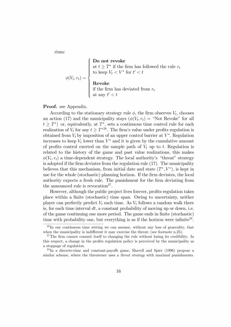
rium:
φ(Vt, rt) =
Do not revokeat t ≥ T ∗ if the firm has followed the rule rtto keep Vt < V ∗ for t0 < t
Revokeif the firm has deviated from rtat any t0 < t
Proof. see Appendix.According to the stationary strategy rule φ, the firm observes Vt, chooses
an action (17) and the municipality stays (φ(Vt, rt) = “Not Revoke” for allt ≥ T ∗) or, equivalently, at T ∗, sets a continuous time control rule for eachrealization of Vt for any t ≥ T ∗26. The firm’s value under profits regulation isobtained from Vt by imposition of an upper control barrier at V ∗. Regulationincreases to keep Vt lower than V ∗ and it is given by the cumulative amountof profits control exerted on the sample path of Vt up to t. Regulation isrelated to the history of the game and past value realizations, this makesφ(Vt, rt) a time-dependent strategy. The local authority’s “threat” strategyis adopted if the firm deviates from the regulation rule (17). The municipalitybelieves that this mechanism, from initial date and state (T ∗, V ∗), is kept inuse for the whole (stochastic) planning horizon. If the firm deviates, the localauthority expects a fresh rule. The punishment for the firm deviating fromthe announced rule is revocation27.However, although the public project lives forever, profits regulation takes
place within a finite (stochastic) time span. Owing to uncertainty, neitherplayer can perfectly predict Vt each time. As Vt follows a random walk thereis, for each time interval dt, a constant probability of moving up or down, i.e.of the game continuing one more period. The game ends in finite (stochastic)time with probability one, but everything is as if the horizon were infinite28.26In our continuous time setting we can assume, without any loss of generality, that
when the municipality is indifferent it may exercise the threat; (see footnote n.25).27The firm cannot commit itself to changing the rule without losing its credibility. In
this respect, a change in the profits regulation policy is perceived by the municipality asa stoppage of regulation.28In a discrete-time and constant-payoffs game, Shavell and Spier (1996) propose a
similar scheme, where the threatener uses a threat strategy with maximal punishments.
16
Proposition Part II (Regulation timing). As long as Vt < V ∗ nothingis done. The first time Vt crosses from below V ∗, at T ∗ = inf(t ≥0 | Vt − V ∗ = 0+), the firm regulates profits using (17) to keep themunicipality indifferent to revoking. Regulation goes on up to the pointwhere the unregulated firm’s value Vt crosses from above the trigger V ∗
and the authority becomes (again) indifferent, i.e. T ∗0 = inf(t ≥ T ∗ |Vt − V ∗ = 0−).
Proof. see Appendix.Since the authority’s strategy is time-dependent, the firm cannot decide
whether to continue or stop the regulation referring only to the current re-alization of Vt. If the regulated value Vt − rt goes below V ∗, in the interval[T ∗, T ∗0) the firm may be willing to stop regulating profits to increase itsvalue. However, for the sake of perfectness, earlier interruption is not al-lowed before T ∗0. Earlier interruptions are not feasible as long as the threatof contract closure is credible. The credibility relies on the fact that themunicipality’s option to revoke if the firm deviates from rt is always worthexercising at Vt ≥ V ∗, i.e. Fm(Vt) ≥ Fm(V ∗). At T ∗0, however, the firm isable to restore the process Vt and the game can start afresh. The timing ofthe game is shown in figure 1 below.
Figure 1 about here
4 Discussion and Policy ImplicationsAlthough our regulation mechanism is simple in nature, several novel impli-cations follow from our analysis. We summarize the discussions of our resultsin the following items.
• Profit-sharing and price adjustment
As argued by Lyon (1996) and Crew and Kleindorfer (1996), most ofthe PCR plans implemented in recent years for monopoly regulation do not
Our continuous time framework calls for a refinement of the threat strategy as in footnoten.25.
17
simply cap prices. To prevent firms’ profits increasing excessively, they alsoinclude limits, called deadbands, on how much firms can gain before trig-gering profit-sharing with customers29. In practice, these regulation plansrequire, in the event of the firm’s profits going beyond a “pre-determined”level, the x factor to be automatically adjusted upward, making the pricecap adjustment rate RPI − x more stringent30.What is the profit deadband that should trigger revision of the price cap
mechanism? And what should the revision level of the x factor be to optimisethe expected welfare? The model presented above helps us to answer thesequestions31.First of all, it is worth stressing that the profit-sharing rule (17) is endoge-
nous: it rises as optimal response from the continuous relationship betweenthe firm and the municipality. Second, this rule is dynamic in nature: sucha repetition of the relationship implicitly establishes the terms of a long-term contract which guarantees the firm with an “allowed” level of profits.Third, the optimal deadband is given by V ∗ (or V ∗ /I): the firm’s value isallowed to evolve according to the geometric Brownian motion (6) until V ∗
is reached. At V ∗ the price adjustment rule RPI − x is revised to stop theprocess Vt from going above V ∗. From this moment onwards the Brownianmotion describing the regulated profits is given by (16), i.e.:
dVt =hαθ + ξ(RPI − x0)
iVtdt+ σVtdWt, V0 = V, for V ∈ (0, V ∗] (18)
29Among those favourable to proft-sharing see also Sappington and Sibley (1992); Sap-pington and Weisman (1996); Burns, Turvey and Weyman Jones (1998).30Although some authors have called this variation of the PCR a “sliding-scale” reg-
ulation (Lyon, 1996; Sappington and Weisman, 1996), we prefer to call it PCR with aprofit-sharing clause as variation of the x factor in the price cap mechanism serves toredistribute rents to customers, making the regulation more ”fair”. We maintain theterm “sliding scale” regulation - as proposed by Joskow and Schmalensee (1986) - for amechanism that encompasses ROR and PCR.31Lyon (1996) in a static model explores the efficiency property of regulatory schemes
that contemplate profit-sharing. He argues that total welfare can always be increased byswitching from a scheme of pure PCR to one with sharing. Crew and Kleindorfer (1996)propose that the x factor be determined with a bargaining process between the firm andthe regulator in the same way as the “allowed” rate of return is determined in the costsof service regulation.
18
where x0 = x −d inf0≤v≤t
(V ∗/Vv)/dt
ξ inf0≤v≤t
(V ∗/Vv) > x is the endogenous new price decrease
factor32. Fourth, by the regulatory profit restriction x0 the probability of anincrease in the firm value decreases as the firm value rises (Teisberg, 1994).Let’s now discuss in detail the price adjustment behind the profit-sharing
rule (17). Once the numerical value for V ∗ is known, by using (3) and (4),the optimal policy (14) can be written as Π(pt)θt =
β1β1−1(ρ−α)I, from which
the boundary value for θ∗ is given by:
θ∗(pt) =β1
β1 − 1(ρ− α)
I
Π(pt)(19)
For any given value of the price cap pt, random fluctuations of θt movethe point (θt, pt) horizontally to the left or right. If the point goes to theright of the boundary, then a price reduction is immediately undertaken, i.e.pt ≤ pt, so that the point shifts down to the boundary. If θt stays on theleft of the boundary, no new price regulation is undertaken. Price reductionproceeds gradually to maintain (19) as an equality. For example, settingRPI − x = 0 so that pt = p, by inverting (19) we can obtain the optimalboundary function p(θt) which determines the optimal price regulation as afunction of the sole state variable θt and the parameter of the problem ξ :
pt = p
Ãθ∗
θt
!1/ξwith
dptdθt
< 0 (20)
The boundary function for this case is shown in Figure 2.
Figure 2 about here
• Sliding scale regulation32Panteghini and Scarpa (2001) consider a similar problem in a continuous time stochas-
tic model of investment choices by a regulated firm. However, in their model the RPI−xrule remains in place as long as profits are below an exogenously given level V , and, ifVt > V , the price decrease factor increases exogenously from x to x0.
19
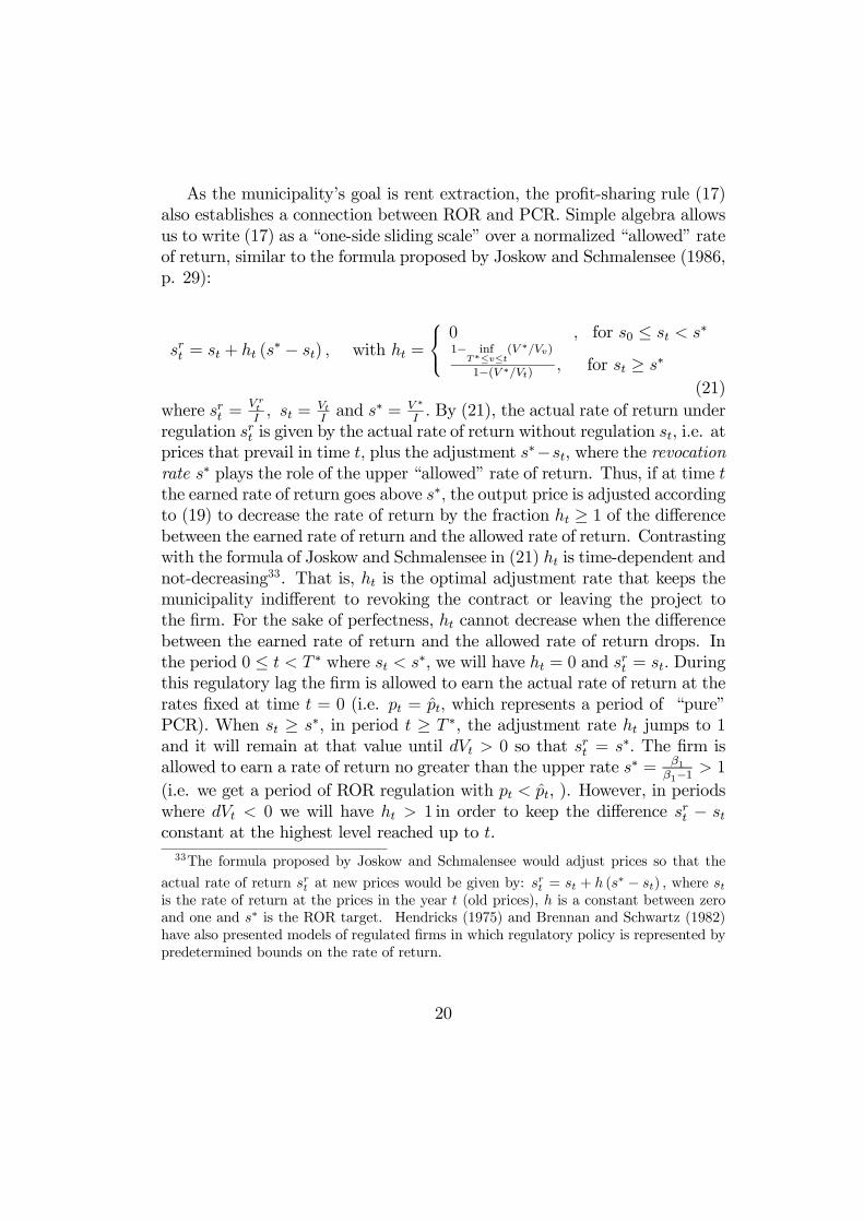
As the municipality’s goal is rent extraction, the profit-sharing rule (17)also establishes a connection between ROR and PCR. Simple algebra allowsus to write (17) as a “one-side sliding scale” over a normalized “allowed” rateof return, similar to the formula proposed by Joskow and Schmalensee (1986,p. 29):
srt = st + ht (s∗ − st) , with ht =
0 , for s0 ≤ st < s∗1− inf
T∗≤v≤t(V ∗/Vv)
1−(V ∗/Vt) , for st ≥ s∗(21)
where srt =V rtI, st =
VtIand s∗ = V ∗
I. By (21), the actual rate of return under
regulation srt is given by the actual rate of return without regulation st, i.e. atprices that prevail in time t, plus the adjustment s∗−st, where the revocationrate s∗ plays the role of the upper “allowed” rate of return. Thus, if at time tthe earned rate of return goes above s∗, the output price is adjusted accordingto (19) to decrease the rate of return by the fraction ht ≥ 1 of the differencebetween the earned rate of return and the allowed rate of return. Contrastingwith the formula of Joskow and Schmalensee in (21) ht is time-dependent andnot-decreasing33. That is, ht is the optimal adjustment rate that keeps themunicipality indifferent to revoking the contract or leaving the project tothe firm. For the sake of perfectness, ht cannot decrease when the differencebetween the earned rate of return and the allowed rate of return drops. Inthe period 0 ≤ t < T ∗ where st < s∗, we will have ht = 0 and srt = st. Duringthis regulatory lag the firm is allowed to earn the actual rate of return at therates fixed at time t = 0 (i.e. pt = pt, which represents a period of “pure”PCR). When st ≥ s∗, in period t ≥ T ∗, the adjustment rate ht jumps to 1and it will remain at that value until dVt > 0 so that srt = s∗. The firm isallowed to earn a rate of return no greater than the upper rate s∗ = β1
β1−1 > 1(i.e. we get a period of ROR regulation with pt < pt, ). However, in periodswhere dVt < 0 we will have ht > 1 in order to keep the difference srt − stconstant at the highest level reached up to t.33The formula proposed by Joskow and Schmalensee would adjust prices so that the
actual rate of return srt at new prices would be given by: srt = st + h (s
∗ − st) , where stis the rate of return at the prices in the year t (old prices), h is a constant between zeroand one and s∗ is the ROR target. Hendricks (1975) and Brennan and Schwartz (1982)have also presented models of regulated firms in which regulatory policy is represented bypredetermined bounds on the rate of return.
20
The non-decreasing property of ht makes the one-side sliding scale (21)similar to an “insurance premium” based on the rate of return st, paid incontinuous time and in advance by the firm to avoid revocation. The firmstarts paying the first time st goes above s∗ (the first occurrence time) andcannot stop or reduce it since this would cancel its coverage. It continuespaying even when “things get better” (profits decrease as well as the munic-ipality’s option value of revoking the contract) in order to have the optionof being active next time the value goes above s∗. When the firm’s currentrate of return goes again above s∗ (the second occurrence time), the firm willbe asked to increase its premium to maintain the coverage. It follows thatthe new regulation is higher, since the firm pays the premium due after the“second occurrence” (see figure 3 in the Appendix).
• Revocation as consistent regulatory policy
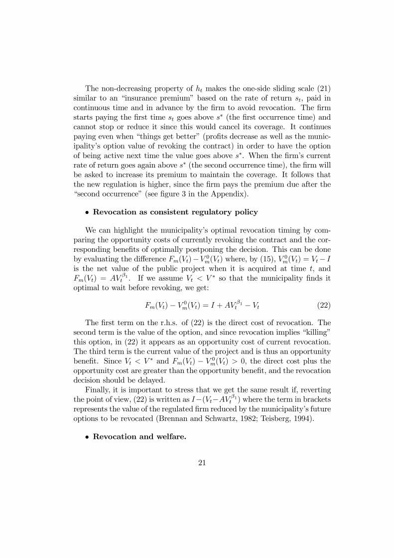
We can highlight the municipality’s optimal revocation timing by com-paring the opportunity costs of currently revoking the contract and the cor-responding benefits of optimally postponing the decision. This can be doneby evaluating the difference Fm(Vt)−V 0m(Vt) where, by (15), V 0m(Vt) = Vt− Iis the net value of the public project when it is acquired at time t, andFm(Vt) = AV
β1t . If we assume Vt < V ∗ so that the municipality finds it
optimal to wait before revoking, we get:
Fm(Vt)− V 0m(Vt) = I + AV β1t − Vt (22)
The first term on the r.h.s. of (22) is the direct cost of revocation. Thesecond term is the value of the option, and since revocation implies “killing”this option, in (22) it appears as an opportunity cost of current revocation.The third term is the current value of the project and is thus an opportunitybenefit. Since Vt < V ∗ and Fm(Vt) − V 0m(Vt) > 0, the direct cost plus theopportunity cost are greater than the opportunity benefit, and the revocationdecision should be delayed.Finally, it is important to stress that we get the same result if, reverting
the point of view, (22) is written as I−(Vt−AV β1t ) where the term in brackets
represents the value of the regulated firm reduced by the municipality’s futureoptions to be revocated (Brennan and Schwartz, 1982; Teisberg, 1994).
• Revocation and welfare.
21
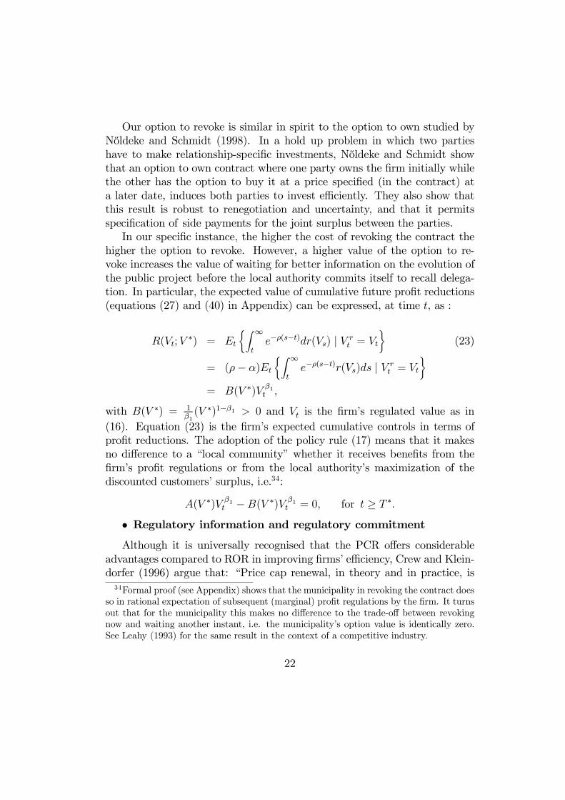
Our option to revoke is similar in spirit to the option to own studied byNoldeke and Schmidt (1998). In a hold up problem in which two partieshave to make relationship-specific investments, Noldeke and Schmidt showthat an option to own contract where one party owns the firm initially whilethe other has the option to buy it at a price specified (in the contract) ata later date, induces both parties to invest efficiently. They also show thatthis result is robust to renegotiation and uncertainty, and that it permitsspecification of side payments for the joint surplus between the parties.In our specific instance, the higher the cost of revoking the contract the
higher the option to revoke. However, a higher value of the option to re-voke increases the value of waiting for better information on the evolution ofthe public project before the local authority commits itself to recall delega-tion. In particular, the expected value of cumulative future profit reductions(equations (27) and (40) in Appendix) can be expressed, at time t, as :
R(Vt;V∗) = Et
½Z ∞te−ρ(s−t)dr(Vs) | V rt = Vt
¾(23)
= (ρ− α)Et
½Z ∞te−ρ(s−t)r(Vs)ds | V rt = Vt
¾= B(V ∗)V β1
t ,
with B(V ∗) = 1β1(V ∗)1−β1 > 0 and Vt is the firm’s regulated value as in
(16). Equation (23) is the firm’s expected cumulative controls in terms ofprofit reductions. The adoption of the policy rule (17) means that it makesno difference to a “local community” whether it receives benefits from thefirm’s profit regulations or from the local authority’s maximization of thediscounted customers’ surplus, i.e.34:
A(V ∗)V β1t −B(V ∗)V β1
t = 0, for t ≥ T ∗.• Regulatory information and regulatory commitmentAlthough it is universally recognised that the PCR offers considerable
advantages compared to ROR in improving firms’ efficiency, Crew and Klein-dorfer (1996) argue that: “Price cap renewal, in theory and in practice, is34Formal proof (see Appendix) shows that the municipality in revoking the contract does
so in rational expectation of subsequent (marginal) profit regulations by the firm. It turnsout that for the municipality this makes no difference to the trade-off between revokingnow and waiting another instant, i.e. the municipality’s option value is identically zero.See Leahy (1993) for the same result in the context of a competitive industry.
22
recognized as the most likely time for PCR to adopt some of the inefficiencesof ROR...(p.212)”. In this regard, it is important to underline the endoge-nous nature of the regulatory lag resulting from our model. In this specificinstance, the price adjustment behind the profit-sharing rule (17) is parame-trized by the deadband V ∗ (or revocation rate s∗ if we refer to (21)). Hence,in addition to the parameters of the model, the key variable for valuing theoption to revoke and thus the municipality’s position during the delegationperiod is the direct cost I which - in turn - depends, excluding indemnities,on training and hiring costs as well as on litigation costs. Thus, informationon production and demand/cost data that the municipality uses to write theregulatory contract are fundamental in determining the length of the reg-ulatory lag. This effect could be weighted with respect to the well-knowntradeoff in ROR literature between a short regulatory lag that promotes al-locative efficiency but is bad for productive efficiency, and a long regulatorylag that produces the opposite effect on allocative and productive efficiency.In the same work, Crew and Kleindorfer (1996) also argue that a ma-
jor issue in incentive regulation is commitment: “If a company is concernedthat the regulator will penalize it at the end of or even during the price-cap period if it is successful, it may not pursue efficiency as strongly asimplied by the apparent incentives of PCR. Thus, the notion that the regu-lator will not renege on the terms of PCR is very important for efficiency tobe achieved....(p.218)”. However, they subsequently admit that as the reg-ulators’ goal is rent extraction it is not difficult to recognise that they havelimited incentives to commit, and that this difficulty is at the base of therecent growth of regulatory contracts which incorporate sharing rules: “Suchdevices provide sharing of gains to ratepayers and therefore might be seen tobe less vulnerable to reneging by the regulator if the company does well. Inaddition, such devices, in limiting how well the company can do, make theregulator less likely to renege....(p.218)”.However, in the process we described in this paper, in addition to the
trade-off between commitment and reneging raised by Crew and Kleindor-fer, it also becomes crucial to highlight the credibility of the municipality topursue these sharing rules, that is to revoke the contract when the revoca-tion trigger V ∗ is reached. This credibility is relevant for the renegotiationprocess itself since it determines the municipality’s bargaining power withthe delegated firm and - in turn - the timing of contract renewal. Indeed, ifthe revocation costs, on the one hand, measure the “inefficiencies” the localauthority incurs by direct management and are, therefore, used to positively
23
evaluate the decision to delegate the public service to a private operator, onthe other hand they raise the problem of the irreversibility of the delegationonce it is made. In the case of local provision of the utilities we refer to, afterthe delegation has taken place the municipal authority plays the role of aregulator with respect to the private firm: the inexperience of the municipalauthority in this role can negatively affect its credibility and thus determinea negotiating disadvantage (Clark and Mondello, 2000).
• Market expectations
As long as public projects are, in general, not traded assets, their growthrate α may actually fall below the equilibrium total expected rate of re-turn α required in the market by investors from an equivalent-risk tradedfinancial security, i.e. δ ≡ α − α > 0 (McDonald and Siegel, 1986). Rely-ing on the asset price equilibrium relationship α − r = λσ, we are able toevaluate the municipality’s value of the option to revoke, replacing α withthe risk-adjusted rate of growth α − λσ = r − δ and behaving as if theworld were risk neutral: where r is the risk-free rate of interest, δ is thebelow-equilibrium return shortfall and λ is the utility’s market price of risk(Brennan and Schwartz, 1982). The allowed rate of return becomes:
s∗ = s∗(r,λ, σ)
Although it seems reasonable to assume that utilities with higher “cap-ital costs” will be allowed to earn higher rates of return, i.e. ∂s∗
∂r> 0, the
empirical evidence that a higher systematic risk, as measured through themarket price of risk λ, results in a higher allowed rate-of-return, i.e. ∂s∗
∂λ> 0
(Fan and Cowing, 1994) is also confirmed. Finally, a higher volatility alsoincreases the allowed rate of return, i.e. ∂s∗
∂σ> 0, but for reasons other than
those related to interest rates and systematic risk. From section 3 we knowthat an increase in the instantaneous variance, σ2, of the revenue processreduces β1 and then increases the option multiply
β1β1−1 . As a result, when
the economic environment becomes more volatile, the market value of thepublic project can go up, but it also increases the municipality’s value ofkeeping the revocation opportunity alive. Thus, the allowed rate of return s∗
is higher since the authority optimal policy is to lag behind in revoking thecontract with the firm.
24
• Final remarks
The paper has modelled the regulation of a local public utility as a long-term relationship between a firm and a municipality. The repetition of therelationship may substitute long-term contracts and guarantee utilities withan appropriate level of profits. Furthermore, since the price and its ad-justment mechanism is contractually fixed when the contract is signed andthe firm is the residual claimant for its profits, a stochastic regulatory lagexists where the regulation has a price cap nature. Excessive revocation costmakes the firm an unregulated monopolist with an infinite regulatory lag.This PCR is followed by a period of ROR in which the firm is induced toadjust its price downward to keep its profits below the allowed level set bythe authority and avoid revocation.
25
A Appendix: The threat gameWe prove that the municipality scheme proposed is a perfect equilibriumbelonging to the class of efficient perfect equilibria (which may be very large)for the continuous time threat-game described in the text.
1) Regulation mechanism
We define the regulation as the negative increment dVt to let Vt stay atV ∗,that is, a policy control is a process Z = {Zt, t ≥ 0} and a regulatedprocess V r = {V rt , t ≥ 0} such that
V rt ≡ VtZt, for V rt ∈ (0, V ∗], (24)
where:
• i) Vt is a geometric Brownian motion, with stochastic differential as in(6);
• ii) Zt is a decreasing and continuous process with respect to Vt ;• iii) Z0 = 1 if V0 ≤ V ∗, and Z0 = V ∗/V0 if V0 > V ∗ so that V r0 = V ∗;• iv) Zt decreases only when V rt = V ∗.
Applying Ito’s lemma to (24), we get:
d V rt = αV rt dt+ σV rt dWt + Vrt
dZtZt, V r0 ∈ (0, V ∗]
where V rtdZtZt≡ VtdZt = −drt is the infinitesimally small level of value given
up by the firm. In terms of the regulated process V rt , we can write:
rt ≡ r(Vt) = Vt − V rt ≡ (1− Zt)Vt, (25)
Although the process Zt may have a jump at time t = 0 it is continuousand maintains Vt below the barrier using the minimum amount of control, inthat control takes places only when Vt crosses V ∗ from below with probabilityone in the absence of regulation. Therefore, in the case of V0 < V ∗, we getV rt ≡ Vt, with initial condition V r0 ≡ V0 = V, and Zt = 1. At T ∗ ≡ T (V ∗) =inf(t ≥ 0 | Vt − V ∗ = 0+) the regulation starts so as to maintain V rt = V ∗.
26
The firm regulates the project’s value by the amount rt = Vt− V rt ≥ 0 everytime V ∗ is hit.Finally, the same conditions (i)− (iv) uniquely determine Zt with the repre-sentation form (Harrison,1985; proposition 3, p. 19-20):35
Zt ≡ min(1, V ∗/V0) for t = 0
inf0≤v≤t(V
∗/Vv) for t ≥ 0 (26)
Figure 3 about here
2) Cost of regulation
Let’s now indicate with R(V r;V ∗) the expected value of future cumulativelosses in terms of the firm’s value due to the regulation. The rational playerevaluates R considering an infinite life project:
R(V r0 ;V∗) = E0
½Z ∞0e−ρtdr(Vt) | V r0 ∈ (0, V ∗]
¾(27)
= −E0½Z ∞
0e−ρtVtdZt] | V r0 ∈ (0, V ∗]
¾Since V rt is a Markov process in levels (Harrison, 1985, proposition 7, p.80-81), we know that the above conditional expectation is in fact a functionsolely of the starting state.36 Keeping the dependence of R on V rt active35This is an application of a well-known result by Levy (1948), for which the process:
lnV rt ≡ lnVt + lnZt ≡ lnVt − inf0≤v≤t
(lnVv − lnV ∗)
has the same distribution as the “reflected Brownian process” | lnVt − lnV ∗ | .36For V0 = V > V ∗ optimal control would require Z to have a jump at zero so as to
ensure V r0 = V ∗. In this case the integral on the right of (27) is defined to include thecontrol cost r0 incurred at t = 0, that is (see Harrison 1985, p.102-103):Z ∞
0
e−ρtdrt ≡ r0 +Z(0,∞)
e−ρtdrt
where r0 = V − V r0 .
27

and assuming that it is twice continuously differentiable, by Ito’s lemma weget:
dR = R0dV rt +1
2R00(dV rt )
2 (28)
= R0(ZtdVt + VtdZt) +1
2R00Z2t (dVt)
2
= R0(αV rt dt+ σV rt dWt + Vrt
dZtZt) +
1
2R00Z2t σ
2dt
=1
2R00σ2V r2t dt+R
0αV rt dt+R0σV rt dWt +R
0V rtdZtZt
where it has been taken into account that for a finite-variation process likeZt,(dZt)2 = 0. As dZt = 0 except when V rt = V
∗ we are able to rewrite (28)as:
dR(V rt ;V∗) = [
1
2σ2V r2t R
00(V rt ;V∗) + αV rt R
0(V rt ;V∗)]dt (29)
+σV rt R0(V rt ;V
∗) dWt −R0(V ∗;V ∗)dr(Vt)
This is a stochastic differential equation in R. Integrating by part the processRe−rt we get (Harrison, 1985, p.73):
e−ρtR(V rt ;V∗) = R(V r0 ;V
∗)+ (30)
+Z t
0e−ρs
·1
2σ2V r2s R
00(V rs ;V∗) + αV rs R
0(V rs ;V∗)− ρR(V rs ;V
∗)¸ds
+σZ t
0e−ρsV rs R
0(V rs ;V∗) dWs − R0(V ∗;V ∗)
Z t
0e−ρsdr(Vs)
Taking the expectation of (30) and letting t→∞, if the following conditionsapply:
(a) liml→0Pr[T (l) < T (V ∗) | V r0 ∈ (0, V ∗]] = 0 for l ≤ V rt < V ∗ < ∞, where
T (l) = inf(t ≥ 0 | V rt = l) and T (V ∗) = inf(t ≥ 0 | V rt = V ∗);(b) R(V rt ;V
∗)) is bounded within (0, V ∗];
28
(c) e−ρtV rt R0(V rt ;V
∗) is bounded within (0, V ∗];
(d) R0(V ∗;V ∗) = 1;
(e) 12σ2V r2t R
00(V rt ;V∗) + αV rt R
0(V rt ;V∗)− ρR(V rt ;V
∗) = 0,
we obtain R(V r;V ∗) as indicated in (27). Condition (a) says that the prob-ability that the regulated process V rt reaches zero before reaching anotherpoint within the set (0, V ∗] is zero. As V rt is a geometric type of process thiscondition is, in general, always satisfied (Karlin and Taylor, 1981, p. 228-230). Furthermore, if condition (a) holds and R(V r;V ∗) is bounded thenconditions (b) and (c) also hold. According to the linearity of (e) and using(d), the general solution has the form:
R(V r0 ;V∗) = B(V ∗)(V r0 )
β1 , (31)
with:
B(V ∗) =1
β1(V ∗)1−β1 > 0. (32)
As for V0 ≤ V ∗, Z0 = 1 and V r0 = V0 = V, then R(V r0 ;V∗) = R(V ;V ∗).
On the other hand, if V0 > V ∗, we get Z0 = V ∗/V0, so that V r0 = V ∗ andR(V r0 ;V
∗) = R(V ∗;V ∗).
3) The value of revocation
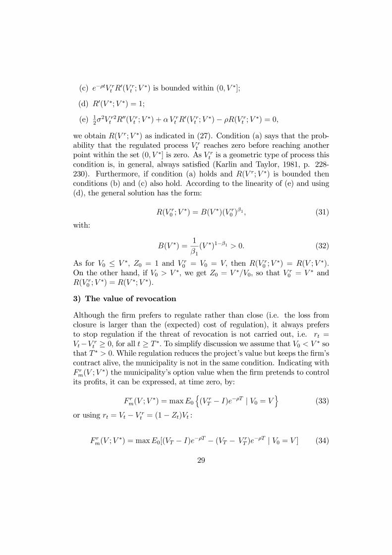
Although the firm prefers to regulate rather than close (i.e. the loss fromclosure is larger than the (expected) cost of regulation), it always prefersto stop regulation if the threat of revocation is not carried out, i.e. rt =Vt−V rt ≥ 0, for all t ≥ T ∗. To simplify discussion we assume that V0 < V ∗ sothat T ∗ > 0.While regulation reduces the project’s value but keeps the firm’scontract alive, the municipality is not in the same condition. Indicating withF rm(V ;V
∗) the municipality’s option value when the firm pretends to controlits profits, it can be expressed, at time zero, by:
F rm(V ;V∗) = maxE0
n(V rT − I)e−ρT | V0 = V
o(33)
or using rt = Vt − V rt = (1− Zt)Vt :
F rm(V ;V∗) = maxE0[(VT − I)e−ρT − (VT − V rT )e−ρT | V0 = V ] (34)
29
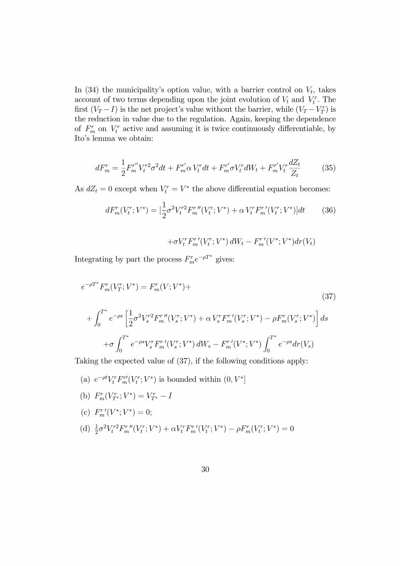
In (34) the municipality’s option value, with a barrier control on Vt, takesaccount of two terms depending upon the joint evolution of Vt and V rt . Thefirst (VT −I) is the net project’s value without the barrier, while (VT −V rT ) isthe reduction in value due to the regulation. Again, keeping the dependenceof F rm on V
rt active and assuming it is twice continuously differentiable, by
Ito’s lemma we obtain:
dF rm =1
2F r
00m V
r2t σ2dt+ F r
0mαV rt dt+ F
r0mσV rt dWt + F
r0mV
rt
dZtZt
(35)
As dZt = 0 except when V rt = V∗ the above differential equation becomes:
dF rm(Vrt ;V
∗) = [1
2σ2V r2t F
rm00(V rt ;V
∗) + αV rt Frm0(V rt ;V
∗)]dt (36)
+σV rt Frm0(V rt ;V
∗) dWt − F rm0(V ∗;V ∗)dr(Vt)
Integrating by part the process F rme−ρT ∗ gives:
e−ρT∗F rm(V
rT ;V
∗) = F rm(V ;V∗)+
(37)
+Z T ∗
0e−ρs
·1
2σ2V r2s F
rm00(V rs ;V
∗) + αV rs Frm0(V rs ;V
∗)− ρF rm(Vrs ;V
∗)¸ds
+σZ T ∗
0e−ρsV rs F
rm0(V rs ;V
∗) dWs − F rm0(V ∗;V ∗)Z T ∗
0e−ρsdr(Vs)
Taking the expected value of (37), if the following conditions apply:
(a) e−ρtV rt Fr0m(V
rt ;V
∗) is bounded within (0, V ∗]
(b) F rm(VrT ∗;V
∗) = V rT ∗ − I(c) F rm
0(V ∗;V ∗) = 0;
(d) 12σ2V r2t F
rm00(V rt ;V
∗) + αV rt Frm0(V rt ;V
∗)− ρF rm(Vrt ;V
∗) = 0
30
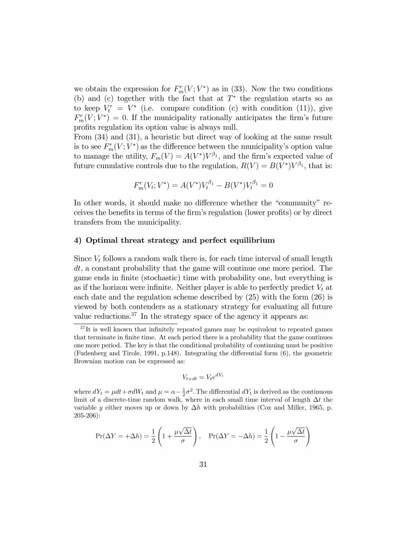
we obtain the expression for F rm(V ;V∗) as in (33). Now the two conditions
(b) and (c) together with the fact that at T ∗ the regulation starts so asto keep V rt = V ∗ (i.e. compare condition (c) with condition (11)), giveF rm(V ;V
∗) = 0. If the municipality rationally anticipates the firm’s futureprofits regulation its option value is always null.From (34) and (31), a heuristic but direct way of looking at the same resultis to see F rm(V ;V
∗) as the difference between the municipality’s option valueto manage the utility, Fm(V ) = A(V ∗)V β1 , and the firm’s expected value offuture cumulative controls due to the regulation, R(V ) = B(V ∗)V β1, that is:
F rm(Vt;V∗) = A(V ∗)V β1
t − B(V ∗)V β1t = 0
In other words, it should make no difference whether the “community” re-ceives the benefits in terms of the firm’s regulation (lower profits) or by directtransfers from the municipality.
4) Optimal threat strategy and perfect equilibrium
Since Vt follows a random walk there is, for each time interval of small lengthdt, a constant probability that the game will continue one more period. Thegame ends in finite (stochastic) time with probability one, but everything isas if the horizon were infinite. Neither player is able to perfectly predict Vt ateach date and the regulation scheme described by (25) with the form (26) isviewed by both contenders as a stationary strategy for evaluating all futurevalue reductions.37 In the strategy space of the agency it appears as:37It is well known that infinitely repeated games may be equivalent to repeated games
that terminate in finite time. At each period there is a probability that the game continuesone more period. The key is that the conditional probability of continuing must be positive(Fudenberg and Tirole, 1991, p.148). Integrating the differential form (6), the geometricBrownian motion can be expressed as:
Vt+dt = VtedYt
where dYt = µdt+σdWt and µ = α− 12σ
2.The differential dYt is derived as the continuouslimit of a discrete-time random walk, where in each small time interval of length ∆t thevariable y either moves up or down by ∆h with probabilities (Cox and Miller, 1965, p.205-206):
Pr(∆Y = +∆h) =1
2
Ã1+
µ√∆t
σ
!, Pr(∆Y = −∆h) = 1
2
Ã1− µ
√∆t
σ
!
31
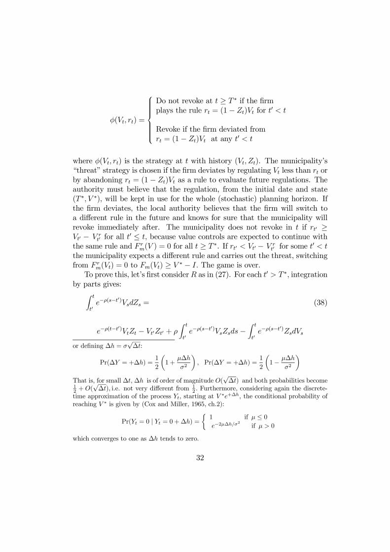
φ(Vt, rt) =
Do not revoke at t ≥ T ∗ if the firmplays the rule rt = (1− Zt)Vt for t0 < t
Revoke if the firm deviated fromrt = (1− Zt)Vt at any t0 < t
where φ(Vt, rt) is the strategy at t with history (Vt, Zt). The municipality’s“threat” strategy is chosen if the firm deviates by regulating Vt less than rt orby abandoning rt = (1− Zt)Vt as a rule to evaluate future regulations. Theauthority must believe that the regulation, from the initial date and state(T ∗, V ∗), will be kept in use for the whole (stochastic) planning horizon. Ifthe firm deviates, the local authority believes that the firm will switch toa different rule in the future and knows for sure that the municipality willrevoke immediately after. The municipality does not revoke in t if rt0 ≥Vt0 − V rt0 for all t0 ≤ t, because value controls are expected to continue withthe same rule and F rm(V ) = 0 for all t ≥ T ∗. If rt0 < Vt0 − V rt0 for some t0 < tthe municipality expects a different rule and carries out the threat, switchingfrom F rm(Vt) = 0 to Fm(Vt) ≥ V ∗ − I. The game is over.To prove this, let’s first considerR as in (27). For each t0 > T ∗, integration
by parts gives:Z t
t0e−ρ(s−t
0)VsdZs = (38)
e−ρ(t−t0)VtZt − Vt0Zt0 + ρ
Z t
t0e−ρ(s−t
0)VsZsds−Z t
t0e−ρ(s−t
0)ZsdVs
or defining ∆h = σ√∆t:
Pr(∆Y = +∆h) =1
2
µ1+
µ∆h
σ2
¶, Pr(∆Y = +∆h) =
1
2
µ1− µ∆h
σ2
¶That is, for small ∆t, ∆h is of order of magnitude O(
√∆t) and both probabilities become
12 + O(
√∆t), i.e. not very different from 1
2 . Furthermore, considering again the discrete-time approximation of the process Yt, starting at V ∗e+∆h, the conditional probability ofreaching V ∗ is given by (Cox and Miller, 1965, ch.2):
Pr(Yt = 0 | Yt = 0 +∆h) =½1 if µ ≤ 0e−2µ∆h/σ
2
if µ > 0
which converges to one as ∆h tends to zero.
32
Taking expectation of both sides and using the zero expectation property ofthe Brownian motion (Harrison, 1985, p.62-63), we have:
Et0Z t
t0e−ρ(s−t
0)VsdZs = Et0[VtZte−ρ(t−t0)]−Vt0Zt0+(ρ−α)Et0
Z t
t0e−ρ(s−t
0)VsZsds
(39)By the Strong Markov property of V rt
38, it follows that Et0[VtZte−ρ(t−t0)] =
Et0 [VtZt]Et0[e−ρ(t−t0)] = V ∗Et0 [e−ρ(t−t
0)]→ 0 almost surely as t→∞, so that:
Et0Z ∞t0e−ρ(s−t
0)VsdZs = −Vt0Zt0 + (ρ− α)Et0Z ∞t0e−ρ(s−t
0)(Vs − rs)ds
Since −Vt0Zt0 + (ρ − α)Et0R∞t0 e
−ρ(s−t0)Vsds = 0, substituting in (27) andrearranging we get:
R(Vt0;V∗) = (ρ− α)Et0
Z ∞t0e−ρ(s−t
0)rsds (40)
Secondly, let’s assume (t0, t) is an interval in which rs is flat so that V rs ≤ V ∗,and t is the first time in which dZt > 0. Considering the decomposition (39)we can write (40) as:
R(Vt0 ;V∗) = (ρ− α)
½Et0
Z t
t0e−ρ(s−t
0)rsds+ Et0½Z ∞
te−ρ(s−t
0)rsds¾¾
= (ρ− α)½Et0
Z t
t0e−ρ(s−t
0)rsds+ Et0½e−ρ(t−t
0)Z ∞t0e−ρ(s−t
0)r∗sds¾¾
where we have defined V r∗s = V rt+s and r∗s = rt+s − rt for t0 ≤ t. Applying,
again, the Strong Markov Property of V rt we get:
R(Vt0;V∗) = Et0
Z t
t0e−ρ(s−t
0)rsds+ Et0½e−ρ(t−t
0)Et0Z ∞t0e−ρ(s−t
0)∞r∗sds¾
= (ρ− α)Et0Z t
t0e−ρ(s−t
0)rsds+ Et0ne−ρ(t−t
0)R(Vt0;V∗)o
= (ρ− α)Et0Z t
t0e−ρ(s−t
0)rsds+R(Vt0 ;V∗)Et0
ne−ρ(t−t
0)o
Since rs = rt0 ≡ Vt0 − V rt0 for all s ∈ (t0, t) we can simplify the aboveexpression as:38The Strong Markov Property of regulated Brownian motion processes stresses the
fact that the stochastic first passage time t and the stochastic process V rt are independent(Harrison, 1985, proposition 7, p.80-81).
33
R(Vt0;V∗) =
(ρ− α)
ρrt0 =
(ρ− α)
ρ(Vt0 − V rt0 ) (41)
>From (41), any application of controls rt0 < Vt0− V rt0 , leads to a reduction of(40) for all t ≥ t0 and then to F rm(Vt;V ∗) > 0. Furthermore, the firm does notregulate more than rt since, by doing so, it does not increase the probabilityof a delayed closure. It does not pay less, since rt < Vt − V rt induces closuremaking it worse off, i.e. 0 < Vt. Finally, as V rt is a Markov process in levels,it is immediate by (40) that any sub-game beginning at a point at whichrevocation has not taken place is equivalent to the whole game. The strategyφ is efficient for any sub-game starting at an intermediate date and state(t, Vt) . We have sub-game perfection.
6) Non-decreasing path of rt within [T ∗, T 0∗).
So far we have implicitly assumed that, once started at T ∗, the regulationgoes on forever. Earlier interruptions are not feasible as long as the threat ofclosure by the municipality is credible. Credibility relies on the fact that theagency’s option-to-revoke the contract if the firm deviates from rt is alwaysworth exercising at Vt > V ∗, i.e. Fm(Vt) ≥ Fm(V
∗). As the decision rulestrategy depends on the history of the game, the authority expects regulationto continue according to the rule rt and any premature stop could make itno longer subgame-perfect.However, in an optimal Brownian path there is a positive probability of theprimitive process Vt crossing V ∗ again starting at an interior point of therange (V ∗,∞). In this case, the firm may be willing to stop regulation. Thatis, the firm regulates its value until Vt ≥ V ∗, letting the agency expect theregulation to continue in the future according to the same rule rt = (1−Zt)Vt,but when Vt reaches, for the first time after T ∗, a predetermined level, sayV 0 ≤ V ∗, it stops the regulation. The authority will face a jump from zero toFm(V
0) ≤ Fm(V ∗) making the threat of revocation no longer credible.To seethis, consider the possibility of the firm’s regulation terminating at time T 0
with T ∗ < T0<∞, where T 0 = inf(t ≥ T ∗ | Vt ≥ V 0) is the first hitting time
of V 0 ≤ V ∗ when regulation is on. The municipality’s option value startingat any t ∈ [T ∗,∞)can be expressed as:
F rm(Vt;V0) = P (V 0;Vt)Et[F rm(VT 0)e
−r(t−T 0)] + (42)
34
(1− P (V 0;Vt))maxEt[(V rT − I)e−r(t−T )]
where P (V 0;Vt) is the probability of the unregulated process Vt reachingV 0 ≤ V ∗ starting at an interior point of the range (V ∗,∞), which is equal to(Cox and Miller, 1965, p. 232-234):
Pr(T 0 <∞ | Vt) ≡ P (V 0;Vt) =µVtV 0
¶−2µ/σ2
with µ = (α− 12σ2) 39. As the starting point is now any t ∈ (T ∗,∞),we can
immediately see in (42) the dependence on both V rt and Vt. Recalling thatthe option value in the case of regulation is zero and that at time T 0 whenthe contract is revoked it is simply F rm(VT 0) = F
rm(V
0),we get:
F rm(Vt;V0) = P (V 0;Vt)Et[F rm(V
0)e−r(T0−t)]
According to the Strong Markov Property of V rt equation (42) becomes:
F rm(Vt;V0) = P (V 0;Vt)F rm(V
0)µVtV 0
¶β2
(43)
where β2 < 0 is the negative root of (13). Since at t the unregulated process
Vt is greater than V 0 and P (V 0;Vt)³VtV 0
´β2=³VtV 0
´β2−2µ/σ2 ≤ 1, we obtain
F rm(Vt;V0) ≤ F rm(V 0) for all t ∈ [T ∗, T 0), which implies that:
F rm(Vt;V0) = F rm(V
∗)
ÃV 0
V ∗
!β1 µ VtV 0
¶β2−2µ/σ2≤ F rm(V ∗) (44)
Therefore, to avoid revocation the regulation continues until time T 0∗ ≡T 0(V ∗) = inf(t ≥ T ∗ | Vt − V ∗ = 0−) when the trigger V ∗ is hit again (forthe first time) after T ∗. The game ends and can then be restarted afresh.
39This probability is P (V 0;Vt) = 1 for µ ≤ 0, see footnote n. 37.
35
References[1] Bergin J., and W.B. MacLeod, (1993), “Continuous Time Repeated
Games”, International Economic Review, 34, 21-37.
[2] Brennan M.J. and E.S. Schwartz, (1982), “Consistent RegulatoryPolicy under Uncertainty”, Bell Journal of Economics, 13, 506-521.
[3] Brennan T., and J. Boyd, (1997), “Stranded Costs, Takings, andthe Law and Economics of Implicit Contracts”, Journal of RegulatoryEconomics, 11, 41-54.
[4] Carles J., and. J. Dupuis, (1989), Service public local, gestion public,gestion privée, Paris.
[5] Clark E., and G. Mondello, (2000), “An Option Approach toFrench Water Delegation”, Journal of Applied Economics, 3 (2), 325-352.
[6] Cox D.R. and H.D. Miller, (1965), The Theory of StochasticProcess, Chapman and Hall: London.
[7] Crew M. and P. Kleindorfer, (1996), “Incentive Regulation in theUnited Kingdom and United States: some lessons”, Journal of Regula-tory Economics, 9, 211-225.
[8] Demski J.S. and D.E.M. Sappington (1991), “Resolving DoubleHazard Problem with Buyout Agreements”, RAND Journal of Eco-nomics, 22, 232-240.
[9] Dixit A., and R. Pindyck, (1994), Investment under Uncertainty,Princeton University Press: Princeton.
[10] Dosi C., Moretto M. and P. Valbonesi, (2001), “Cost ReductionIncentive and Profit-Sharing regulation”, University of Padova, mimeo.
[11] Fan, D.K., and T.G. Cowing, (1994), “Regulatory Information, Mar-ket Expectations, and the Determination of the Allowed Rate of Re-turn”, Journal of Regulatory Economics, 6, 433-444.
[12] Fudenberg D., and J. Tirole, (1991), Game Theory, The MITPress: Cambridge MA.
36
[13] Gregory S.J. and D.F. Spulber, (1997), Deregulatory Takings andthe Regulatory Contracts, The MIT Press: Cambridge MA.
[14] Harrison J.M., and M.T. Taksar, (1983), “Instantaneous Controlof Brownian Motion”, Mathematics and Operations Research, 8, 439-453.
[15] Harrison J.M., (1985), Brownian Motions and Stochastic Flow Sys-tems, Wiley: New York.
[16] Hendricks W., (1975), “The Effect of Regulation on Collective Bar-gaining in Electric Utilities”, Bell Journal of Economics, 6, 451-465.
[17] Karlin, S. and H.M. Taylor, (1981), A Second Course in StochasticProcesses, Academic Press: New York.
[18] Klein D., and B.O. Flaherty, (1993), “A game Theoretic Renderingof Promises and Threats”, Journal of Economic Behavior and Organi-zation, 21, 295-314.
[19] Joskow P., (1973), “Pricing Decisions of Regulated Firms: A Behav-ioral Approach”, Bell Journal of Economics, 4, 118-140.
[20] Joskow P., and R. Schmalensee, (1986), “Incentive
Regulation for Electric Utilities”, Yale Journal on Regulation, 4, 1-49.
[21] Laffont J. and J. Tirole, (1994): A Theory of Incentives in PublicProcurement and Regulation, The Mit Press: Cambridge MA.
[22] Leahy, J. P., (1993), “Investment in Competitive Equilibrium: theOptimality of Myopic Behavior”, Quarterly Journal of Economics, 108,1105-1133.
[23] Levy P., (1948), Processus Stochastiques et Mouvement Brownien,Gauthier-Villars: Paris.
[24] Lyon T.P., (1996), “A Model of Sliding-Scale Regulation”, Journal ofRegulatory Economics, 9, 227-247.
[25] Lyon T.P. and H. Huang, (2000), “Legal Remedies for Breach of theIncomplete Regulatory ‘Contract’.” mimeo.
37
[26] Lorraine D., (1995), Gestions urbaines de l’eau, Economica: Paris.
[27] McDonald R. and D. Siegel, (1986), “The Value of Waiting toInvest”, Quarterly Journal of Economics, 101, 707-727.
[28] Miceli T.J. and K. Segerson, (1994), “Regulatory Takings: WhenShould Compensation be Paid?”, Journal of Legal Studies, 23, 749-776.
[29] Mameli, B. (1998), Servizio Pubblico e Concessione, Giuffrè: Milano.
[30] Marcou, G. (1995), “Les modes de gestion des services public locauxen Allemagne et le problème de l’overture à la concurrence”, RDF adm.,11, 462-496.
[31] Moretto M., and G. Rossini, (1997), “Endogenous Allocation ofthe Exit Option between Workers and Shareholders”, FEEM Note diLavoro n. 76.97, Milan.
[32] Moretto M., and G. Rossini, (2001), “Designing Severance Pay-ments and Decision Rights for Efficient Plant Closure under Profit-Sharing”, in Murat Sertel (ed.) Advances in Economic Design, SpringerVerlag: Berlin (forthcoming).
[33] Noldeke G. and K.M. Schmidt, (1998), “Sequential Investment andOption to Own”, RAND Journal of Economics, 29, 633-653.
[34] Panteghini P. and C. Scarpa, (2001), “Incentives to (Irreversible)Investments under Different Regulatory Regimes”, University of Brescia,mimeo.
[35] Simon L., and M. Stinchcombe, (1989), “Extensive Form Games inContinuous Time: Pure Strategies”, Econometrica, 57, 1171-1214.
[36] Shavell S., and K. Spier, (1996), “Threats without Binding Com-mitments”, NBER Working Paper 5461.
[37] Teisberg E.O., (1994), “An Option Valuation Analysis of InvestmentChoices by a Regulated Firm”, Management Science, 40, 535-548.
38
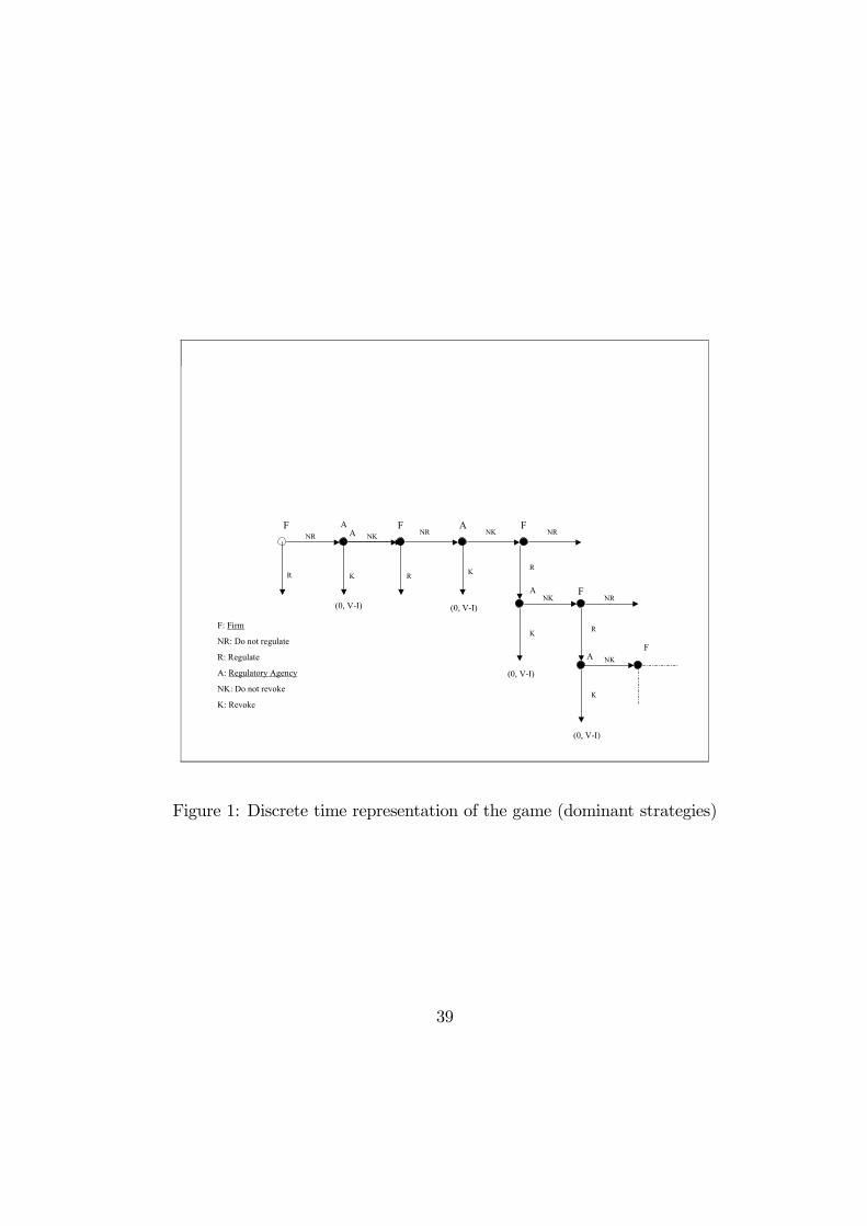
F: Firm
NR: Do not regulate
R: Regulate
A: Regulatory Agency
NK: Do not revoke
K: Revoke
FA F AF
FA
AF
NR
R
NK
K
NR
R
NKA
K
K
NK
K
NK
R
NR
NR
R
(0, V-I) (0, V-I)
(0, V-I)
(0, V-I)
Figure 1: Discrete time representation of the game (dominant strategies)
39
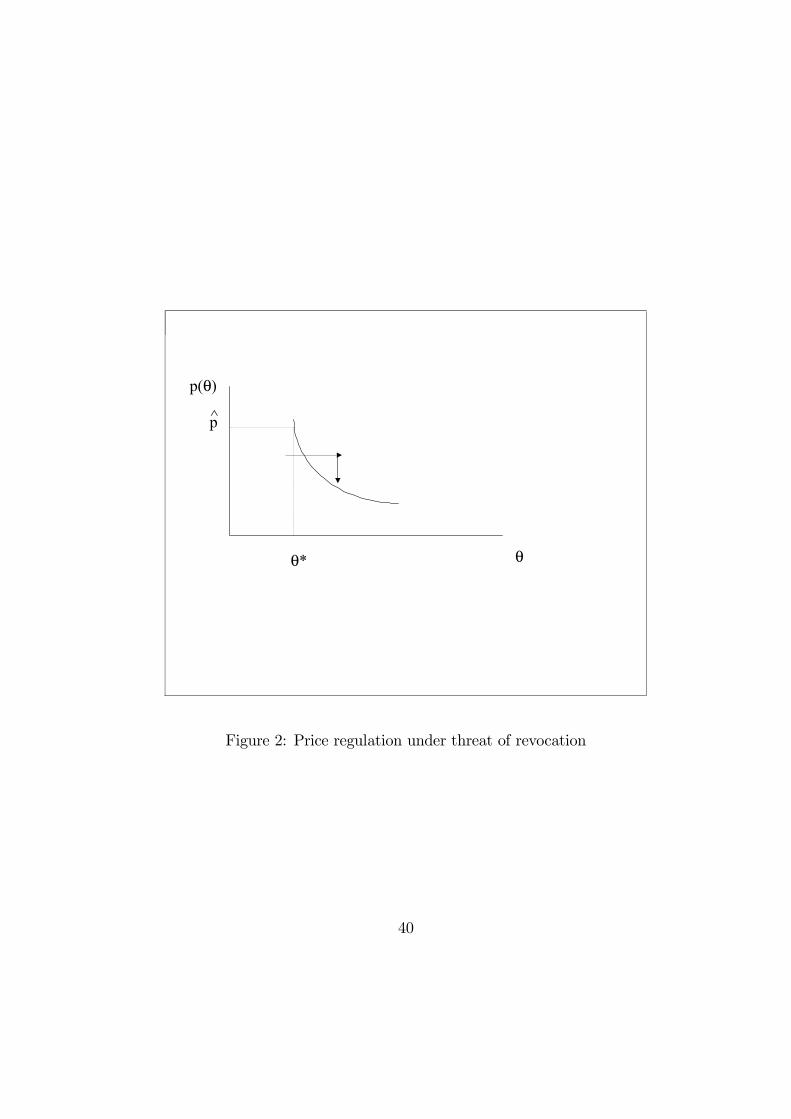
θ
p(θ)
θ*
p
Figure 2: Price regulation under threat of revocation
40
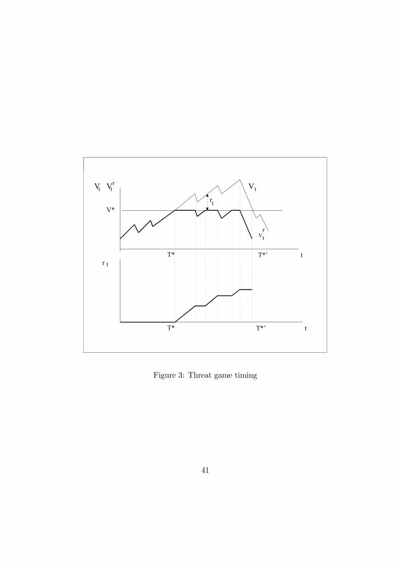
Vt Vtr
V*
T* t
tT*
T*’
T*’
r t
rt
Vt
tr
V
Figure 3: Threat game timing
41