Embed Size (px)
Citation preview
This PDF is a selection from an out-of-print volume from the NationalBureau of Economic Research
Volume Title: Studies in Public Regulation
Volume Author/Editor: Gary Fromm, ed.
Volume Publisher: The MIT Press
Volume ISBN: 0-262-06074-4
Volume URL: http://www.nber.org/books/from81-1
Publication Date: 1981
Chapter Title: Regulation and the Multiproduct Firm: The Case ofTelecommunications in Canada
Chapter Author: Melvyn A. Fuss, Leonard Waverman
Chapter URL: http://www.nber.org/chapters/c11434
Chapter pages in book: (p. 277 - 328)
6Regulation and the Multiproduct Firm:
The Case of Telecommunications in Canada
Melvyn FussLeonard Waverman
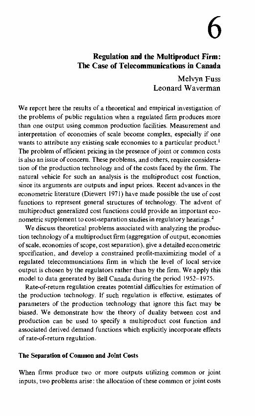
We report here the results of a theoretical and empirical investigation ofthe problems of public regulation when a regulated firm produces morethan one output using common production facilities. Measurement andinterpretation of economies of scale become complex, especially if onewants to attribute any existing scale economies to a particular product.1
The problem of efficient pricing in the presence of joint or common costsis also an issue of concern. These problems, and others, require considera-tion of the production technology and of the costs faced by the firm. Thenatural vehicle for such an analysis is the multiproduct cost function,since its arguments are outputs and input prices. Recent advances in theeconometric literature (Diewert 1971) have made possible the use of costfunctions to represent general structures of technology. The advent ofmultiproduct generalized cost functions could provide an important eco-nometric supplement to cost-separation studies in regulatory hearings.2
We discuss theoretical problems associated with analyzing the produc-tion technology of a multiproduct firm (aggregation of output, economiesof scale, economies of scope, cost separation), give a detailed econometricspecification, and develop a constrained profit-maximizing model of aregulated telecommunciations firm in which the level of local serviceoutput is chosen by the regulators rather than by the firm. We apply thismodel to data generated by Bell Canada during the period 1952-1975.
Rate-of-return regulation creates potential difficulties for estimation ofthe production technology. If such regulation is effective, estimates ofparameters of the production technology that ignore this fact may bebiased. We demonstrate how the theory of duality between cost andproduction can be used to specify a multiproduct cost function andassociated derived demand functions which explicitly incorporate effectsof rate-of-return regulation.
The Separation of Common and Joint Costs
When firms produce two or more outputs utilizing common or jointinputs, two problems arise: the allocation of these common or joint costs

Fuss and Waverman 278
to the separate outputs, and the measurement of aggregate output for thefirm.
Common costs are defined as the costs of common inputs utilized bytwo or more outputs, so that the multiproduct transformation function isrepresented by
(1)
where Yt(i = 1,... ,ra) are outputs and X} (J — 1,... ,n) are inputs. Werecosts not common, (1) could be rewritten as
(2)
where y = \,...,d,...,h,...,k,...,n.
Joint costs as they are defined in the regulation literature occur whentwo or more outputs are produced in fixed proportions; it is impossible toproduce some proportion X of 1 without also producing X of the others(Kahn 1971). The product transformation curve can then be representedas
F{Xu...,Xn) = mm{alYua2Y2,...,amYm). (3)
Note that (3) is the limiting case of (1). In the following discussion wewill treat the problems of common and joint costs as the same issue,referring instead to joint production, as represented by equation (1).Whether costs are "joint" or whether production is characterized byfixed coefficients can be tested empirically.
When a firm produces heterogeneous products, there is no singleunique index of output. For an index h(Y) to be formed, the producttransformation function must be written as
F(Yl,...,Ym,Xu...,Xn) = F{h{Y\Xx,...,Xn). (4)
But (4) can be rewritten as F(h(Y),g(x)) — 0, since the existence of anoutput aggregate implies the existence of an input aggregate (Brown et al.1976; Baumol and Braunstein 1977).3 As a result, the dual joint costfunction is separable in outputs. But then the relative marginal costs ofthe outputs are independent of input prices—a strong assumption (seeLau 1978).

Multiproduct Firms: Telecommunications in Canada 279
Most regulated industries involve joint production. Electric utilitiesproduce peak and off-peak kWh utilizing common generating transmis-sion and distribution capacity. Railroads use the same roadbed forpassenger and freight traffic. Telecommunications firms provide a widevariety of services: residential local switched calls, business local switchedcalls, residential switched toll calls, business switched toll calls, privatewire service, teletypewriter exchange service, specialized common-carrierservice, and a variety of broadband data services. All switched callsutilize local exchange switching equipment in common. Toll calls utilizecommon interoffice switching equipment and common intercity commu-nications equipment. Business switched and nonswitched private wireservices all use common intercity plant. These are but several of the manyexamples of joint production in the telecommunications sector.
It is difficult to find examples of true joint costs in telecommunicationsexcept in a temporal distribution sense. An increase in the number ofcircuits between two points provides increased capacity which is distri-buted between day and night-time calls in fixed proportions. But thissame increase in peak circuit availability can provide a varying proportionof business and residential calls, hence the increase in plant is commonto business and residential use but joint between peak and off-peak use.In the remainder of the paper when we use the term "jointness" we meanin the production sense, encompassing both common and joint costs asused in the regulation literature.
Effective regulation poses the following fundamental questions:
• What range of services is best supplied by a single firm? What are theproduction economies of scale (the change in average and marginalcosts when firm size is increased)?4 What are the economies of scope(the change in average and marginal costs when services are combinedwithin a single firm)?5 Economies of scope exist if and only ifproduction is joint.• What are the long-run marginal costs of producing one more unit ofany one of the joint outputs (Yt,..., Ym)1
The first set of analyses help determine the size of the firm and the degreeof competition to be allowed ;6 the second analysis allows the examinationof the efficiency of any rate structure.
Cost Functions, Economies of Scale, and Economies of Scope
The Multiproduct Cost FunctionA multiproduct production process can be represented by the producttransformation function
Fuss and Waverman 280
..,Ym,Xl,...,Xn) = 0, (5)
where Yt (i = 1,... ,ra) are outputs and Xj(J = 1,... ,«) are inputs.7
In this section we consider only the case where rate-of-retum regulationeither is not used by the regulatory authorities or else is ineffective. Ineither case, we may assume that the firm pursues cost-minimizing behaviorwithout regard to the possibilities of Averch-Johnson-type distortions. Inthat case, the theory of duality between cost and production (see Diewert1971) ensures that for every transformation function of the type shownin equation (1) there exists a dual cost function of the form
C=C(Y1,...,Ym,P1,...,Pn), (6)
where Pj(j — 1,...,«) are the prices paid by the firm for the inputs X}—as long as the product transformation function satisfies the usual regularityconditions (such as convex isoquants), the firm pursues cost-minimizingbehavior, and the firm has no control over input prices.
Under these assumptions, the cost function is just as basic a descriptionof the technology as the product transformation (joint production) func-tion, and it contains all the required information, including informationon jointness.
The properties of the multiproduct cost function (6) are that C isconcave in Pj, linearly homogeneous in P}, and increasing in Y, and Py,that dC/dPj = Xj (Shephard's lemma) ;8 and that the own-price elasticitiesof factor demand are given by
82C/dC£jj~ jdpjl dp;
Economies of Scale and Incremental CostsThe fact that average cost (cost per unit of output) is not defined formultiple-output technologies makes analysis of returns to scale somewhatcomplex, since we can no longer just measure the effect of output increaseson the average cost of production. In addition, we need to distinguishbetween economies of scale in some overall sense (that is, when all outputsare increased) and economies of scale associated with the expansion of aparticular output (with all other outputs held constant). We begin byconsidering an overall measure of returns to scale.
"Overall" returns to scale can be obtained by computingm r\C
dC = I §dY,i=l v Ii

Multiproduct Firms: Telecommunications in Canada 281
or
Equation (7) represents the total change in cost resulting from differentialchanges in the levels of the m outputs. Unfortunately, unless we addadditional structure to equation (7) it is difficult to interpret changes incost resulting from changes in outputs in terms of returns to scale. Onecommon procedure is to assume that all outputs are increased in propor-tion; that is, dYi/Yi = d\ogYt = X. Then
( 8 )_ A glogC
If dlogCjX > 1, incremental overall costs are increasing and hence pro-duction is subject to decreasing returns to scale; if d\ogC/X < 1, thetechnology exhibits increasing returns to scale; if dlogCjl — 1, overallconstant returns to scale exist.
This overall description of returns to scale is somewhat less relevantin the multiple-output case than in the single-output case, since it requiresall outputs to be increasing in strict proportion, which may not correspondto the optimal production plan. Nevertheless, the overall-returns-to-scalenumber can be a useful summary statistic for comparing results obtainedfrom the present framework with returns to scale estimated from aggre-gate production or cost functions (that is, functions that aggregate alloutputs into a single variable).
Now consider the concept of returns to scale with respect to a singleoutput. From equation (7),
dlogC = dlogCdlOgY; 31 — ~ - ^
Yj, j # ; constant
The term d logC/d log^, the output cost elasticity, represents incrementalor marginal cost in percentage terms.
It is tempting to specify that if
— —^— > 1,
returns to scale in producing the zth output are decreasing; that if
a logy, K h
Fuss and Waverman 282
they are increasing; and that if
d logy,. = l'
they are constant. This specification would yield the correct trichotomyfor the case of a single-output production process. However, any attemptto use this definition can lead to a conflict with the definition of overallreturns to scale introduced earlier. Consider the two-output Cobb-Douglas cost function
C = AY\>Y°2i. (10)
Overall decreasing returns to scale implies
However, d logC/<3 log = a; can be < 1 while a1 + a2 > 1, which leadsto a contradiction between our overall and the proposed output-specificreturns to scale measures. Thus, we must reject the use of the individual-product cost elasticities as indicators of returns to scale. However, if oneof the cost elasticities exceeds unity, the sum of them will also exceedunity and therefore no contradiction will arise.
Can we define a meaningful indicator of the potential advantages ordisadvantages of output expansion? Since cost elasticity cannot be used,the remaining intuitive concept is that of changes in incremental cost. Itwould appear, at first glance, that decreasing incremental cost (d2C/dYf< 0) should indicate increasing returns to scale. However, we will showthat this marginal-cost concept also does not provide a solution to theproblem of developing an unambigous indicator of scale economies. Itcan easily be shown that
(12)c [d2\ogc diogc fd\ogcdY? YThe usual situation is that dlogC/dlogy, < 1. The more disaggregatedthe output vector, the more likely it is that 8 logC/d log Yt < 1. If we acceptthis case, then an additional sufficient condition for d2C/dY? < 0 is thatd2 logC/dlogyf < 0; that is, that cost elasticity is a decreasing functionof output. In all such cases, a highly possible outcome is that marginalcosts with respect to each output will decrease (d2C/dY? < 0) and, at thesame time, overall returns to scale will also decrease (Lj(d \ogC/d \ogYt)> 1). In addition, for any given degrees of jointness and overall returns
Multiproduct Firms: Telecommunications in Canada 283
to scale, it is possible (for the case of decreasing cost elasticity) to increasethe rate at which marginal costs decline simply by further disaggregationof the outputs. These two possibilities should be sufficient warning againstusing any observed decreasing marginal cost as an indicator of sub-product-specific returns to scale. In fact, there exists no unambiguousmeasure of output-specific returns to scale except in the case of nonjointproduction,9 since separate cost functions cannot be constructed whencommon costs exist. Thus, we appear to be left with only the overallmeasure of returns to scale.10 Unfortunately, this measure is of no valuewhen one is attempting to evaluate the possible efficiency gains fromincreasing the scale of production of one of the outputs in a multiproductproduction process.
Joint Production, Economies of Scope, and SubadditivityTo this point we have assumed that the production technology is truly amultiple-output one, in the sense that it is more efficient to produce them outputs together than by separate production processes. This efficiencycondition (jointness in production) is known in the industrial organizationliterature as economies of scope (see Panzer and Willig 1975, 1979; Baumoland Braunstein 1977).
For the purposes of this paper, we will say that the production tech-nology exhibits economies of scope if
C(YX-Ym) < C(F 1 ,0--0) + C(0,F2,0---0) + C(0,0,73 •••())
+ •••+ c(o,o---o,ym). (13)
Panzer and Willig (1979) have shown that a sufficient condition for atwice-differentiable multiproduct cost function to exhibit economies ofscope is that it exhibit cost complementarities, defined by
d2c< o (/ ±j\ij= l,...,m). (14)
Conditions (14) provide a means of testing for the existence of economiesof scope.
In a series of articles, Baumol (1977b), Baumol, Bailey, and Willig(1977), and Panzer and Willig (1977) have established the importance of"subadditivity of the cost function" as a production characteristic in theanalysis of a regulated monopolist. Unfortunately, a test for subadditivityis difficult to devise, since one of the requirements is a knowledge of thecost function in the neighborhood of zero outputs. The closest we can
Fuss and Waverman 284
come is a (weak) local test in the neighborhood of the point of approxima-tion. It can be shown that the simultaneous existence of local eco-nomies of scale and local economies of scope is sufficient to ensure localsubadditivity.
Cost Separation and Econometric Cost Functions
The transcripts of regulatory hearings in the telecommunications sectorare replete with discussions of how to allocate joint and common cost.11'12
In the United States, since some of the telephone plant is under statejurisdiction and some under federal jurisdiction, it became necessary to"separate" interstate from intrastate plant. When regulators became con-cerned with the structure of prices rather then just their average level,costs of different services had to be separated. The push for entry byspecialized common carriers (SCCs) and AT&T's competitive responseprompted the F.C.C. requests for guidance from affected parties. InCanada, competitive pressures between two transnational carriers andsuggestions of "cream skimming" and predatory pricing prompted alengthy cost inquiry.
Three basic separation formulas have been proposed: embedded directcost (EDC), long-run increamental cost (LRIC), and fully distributedcost (FDC). These formulas are needed in order to assess "correct"prices. The FDC method is essentially one of long-run average costpricing. Two methods have been proposed to fully distributed theseaverage costs: relative use (revenue share, for example) and historical costcausation.13
The calculation of average embedded direct costs is equivalent to themeasurement of short-run variable costs. Unless there are no fixed costs,long-run pricing at EDC will generate losses. FDC in principle takes intoaccount the fixed costs. However, pricing on the basis of FDC is associatedwith a number of problems. Where production is characterized by long-run returns to scale, setting price equal to average FDC is inefficientsince, for Pareto optimality, prices ex ante should be set equal to long-runincremental costs. Separating common costs by some measure of relativeuse is arbitrary and should not be used as a basis for price setting, sincethere is in general no connection between intensity of use and costcausation.
Cost separation is a bogus issue that exists because of regulatorycommissions' reliance on historical average costs as a guide to settingprice. But there is no method of correctly separating historical average

Multiproduct Firms: Telecommunications in Canada 285
costs. Pricing rules based on efficiency criteria should be set at long-runincremental costs, thus avoiding any need to "separate" costs.
One must be careful in defining the long run, in order to be certain thatincremental costs are measured in terms of changes in capacity output,not changes in actual output at less than capacity.14 As an example, letus examine the data-telecommunications market. Carriers have arguedthat the incremental costs of data service are low since it is an adjunct tothe large monopoly switched message service that must be provided forvoice transmission. However, if the quality of the entire system must beincreased to accommodate an acceptable level of reliability for datatransmission, these upgrading costs are attributable to data-service usersand should be fully charged to them alone as part of the incrementalcosts of the change in the system. This higher quality of service is providedjointly to all users, but quality-upgrading joint costs should be solelyallocated to the data-service users.
Can econometric analysis of the retrospective cost functions of telecom-munications firms provide useful information for regulatory purposes?In theory, given highly disaggregated data corresponding to true economicvariables in the absence of strong time trends, long-run incremental costscould be allocated on a historical assigned-cause basis.15
Econometric cost function analysis can be used to examine the responseof a firm at the margin; that is, at the replacement values or opportunitycosts of inputs. Costs are minimized subject to current factor prices.Regulators, while allowing the firm to use opportunity costs for laborand materials inputs, insist that the firm earn its allowed rate of returnon the historical cost of the capital stock, not its replacement cost. As aresult, costs and prices as determined under a regime of historical-costrate base will differ from the incremental costs and prices determined byan econometric cost function.16
In a period of inflation, historical costs will be less than replacementcosts. Incremental costs determined econometrically will then exceedhistorical "incremental" costs. One of the purposes of cost separation isto estimate the relative contributions of the various services—that is, theexcess of price over historical cost. Comparing actual prices (those set byregulators on the basis of historical cost) with incremental replacementcosts is no guide in determining the extent of cross-subsidization inherentin the actual price structure (when replacement and historical costsdiffer).
Incremental replacement costs are, however, a guide to efficient pricingbehavior. Where economies of scale are not present, setting the price for

Fuss and Waverman 286
each service equal to the incremental replacement cost (as determined byan econometric cost function) yields the set of subsidy-free Pareto-optimalprices. If there are economies of scale and the firm is constrained to atleast break even, calculating the set of Ramsey prices on the basis of theseincremental replacement costs leads to the most efficient "constrained"set of prices, assuming neutrality in interpersonal comparisons (that is,where distributional consequences are disregarded).
Econometric Specification of a Joint Production Process
Profit-Maximizing Model for a Multioutput Regulated FirmEstimates of demand elasticities indicate that regulated telecommunica-tions firms operate some services in the region of inelastic demand.17 Butprofit-maximizing monopolies will never produce where marginal revenueis negative; to do so would require setting marginal revenue equal tonegative marginal costs. If marginal costs are positive, an unregulatedprofit-maximizing monopoly finding itself in the inelastic region of de-mand would raise price (lower output) to increase total revenue.18 How-ever, many regulated utilities are not able to lower output, since theregulators insist that certain basic services be offered at prices that forcethe monopolist to remain in the inelastic region. One example is passengertrain service. Most railroad firms would wish to reduce passenger serviceand raise its price. However, regulators in North America do not permitrail companies to raise the price of this service to the profit-maximizinglevel, although they do require the provision of passenger seats.
All studies of the telephone industry suggest that local telephone serviceis characterized by inelastic demand. The observed level of local service andthe corresponding price are chosen not by a profit-maximizing monopo-list, but by the regulators. As a result, it is reasonable to assume that theobserved level of local service is not an endogenous choice variable to thefirm. Instead, we consider the level of local service exogenous to the firm.
The firm's problem is to maximize profits,
7i = ZqiYi-C(Yu...,Ym,Pu...,Pn), (15)
subject to the constraint on the provision of certain services:
Y^Yt (ieH),
where H is the class of outputs constrained by the regulators, assumedto be the first H outputs. (Note that if demand were inelastic in the regionof Yh the firm would never decide to offer more than Y^}9)

Multiproduct Firms: Telecommunications in Canada 287
Substituting into the profit expression, we obtain
i$H ieH
For profit-maximizing behavior we have the first-order conditions
or20
MRt = MC( {i = H + l , . . . ,m).
In addition, the second-order conditions for maximization require that21
dMRt dMQ
dYt - dY{ ' K '
For observed output levels such that demand is elastic, we assume thatmarginal revenue is set equal to marginal cost. For output levels suchthat demand is inelastic, we assume that those outputs are exogenous tothe firm.
The Multiple-Output Translog Cost FunctionThe translog cost function is becoming an increasingly popular specifica-tion of the functional form of a cost function (Brown et al. 1976; andFuss 1977). The function is quadratic in logarithms and is one of thefamily of second-order Taylor-series approximations to an arbitrary costfunction. The multiple-output translog cost function, assuming capital-augmenting technical change (input n), takes the form22
m n — 1
logC = a0 + X a,-logy; + X ftlogPj + ftlogP*
m m n—1n—1
+ i Z I Wog iogn + i z Zi=lfc=l j= l f c= l
n m n — 1
+ i I yjnlogiyog/>* + X I Pylo
(18)t = i
where a0, a,, j97-, Sik, yjk, pu are parameters to be estimated, and P* =Pne~et where 0 is the rate of decline in the price of a nominal unit of

Fuss and Waverman 288
capital due to capital-augmenting technical change. (In all the followingequations, the asterisk notation is dropped unless it is important forinterpretation.)
Using Shephard's lemma (dC/dPj — Xj), we have
= Mj = fij + lyjk\ogPk + Ipylogl^, (19)
where; = l,...,n and M, is the cost share of the 7th input.Equations (18) and (19) make up the cost system. However, a number
of features of the system reduce the number of parameters to be estimated.Since Mj is a cost share,
this implies
= 1. lyjk = 0, j > y = o.
In addition, the linear homogeneity property of cost functions outlinedearlier implies the further parameter restrictions
Finally, the fact that the function is a second-order approximationimplies
The translog cost function can be used along with the profit-maximizingconditions to generate additional equations representing the optimalchoice of endogenous outputs.
Taking the derivations of the cost function with respect to endogenousoutputs, we have23
5C^1 _ MR XL - frO + WYjdYC lClC C '
where e, is the own price elasticity for the /th output. Denoting qt YJC asRt, the "revenue share," we obtain
Multiproduct Firms: Telecommunications in Canada 289
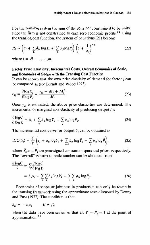
For the translog system the sum of the Rt is not constrained to be unity,since the firm is not constrained to earn zero economic profits.24 Usingthe translog cost function, the system of equations (21) become
Rt = U + 15alogn + Zpijlogp\ (l + ±) \ (22)
where / = H + 1,... ,m.
Factor Price Elasticity, Incremental Costs, Overall Economies of Scale,and Economies of Scope with the Translog Cost FunctionIt can be shown that the own price elasticity of demand for factor j canbe computed as (see Berndt and Wood 1975)
*A"%Xj jjj — Mj + Mj_
jjdlogPj
Once jjj is estimated, the above price elasticities are determined. Theincremental or marginal cost elasticity of producing output / is
| ^ = a, + lSik\ogYk + Xp,,logP,, (24)01OS ri k j
The incremental cost curve for output Yt can be obtained as
L + SulogYt + S 5ik\ogYk + IpylogpJ) , (25)J
where Yk and Pj are preassigned constant outputs and prices, respectively.The "overall" returns-to-scale number can be obtained from
dlogC = y d logC
= Z «.• + Z Z ** lQg n + Z Z PU ^gPj. (26)i k
Economies of scope or jointness in production can only be tested inthe translog framework using the approximate tests discussed by Dennyand Fuss (1977). The condition is that
5tj = -a^j
when the data have been scaled so that all Yt — Pj — 1 at the point ofapproximation.2 5
Fuss and Waverman 290
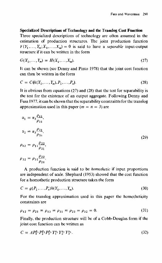
Specialized Descriptions of Technology and the Translog Cost FunctionThree specialized descriptions of technology are often assumed in theestimation of production structures. The joint production functionF(Yi,...,Ym;X1,...,Xm) = 0 is said to have a separable input-outputstructure if it can be written in the form
G(Y1,...,YJ = H(X1,...,XJ. (27)
It can be shown (see Denny and Pinto 1978) that the joint cost functioncan then be written in the form
C= C(h(Y1,...,Ym),P1,...,Pn). (28)
It is obvious from equations (27) and (28) that the test for separability isthe test for the existence of an output aggregate. Following Denny andFuss 1977, it can be shown that the separability constraints for the translogapproximation used in this paper (m = n = 3) are
2 3 >
P 3 1 (29)
P21
P32 = P 3 1 — •P21
A production function is said to be homothetic if input proportionsare independent of scale. Shephard (1953) showed that the cost functionfor a homothetic production structure takes the form
C = g(P1,...,Pn)h(Y1,...,YJ. (30)
For the translog approximation used in this paper the homotheticityconstraints are
P12 = P21 = P13 = P31 = P23 = P32 = 0. (31)
Finally, the production structure will be of a Cobb-Douglas form if thejoint cost function can be written as
c = AP^P^P^ rji y|2 Y^. (32)
Multiproduct Firms: Telecommunications in Canada 291
For the translog function used in this paper the Cobb-Douglas constraintsare
Sik = Pij = 7jk = 0 (i,j,k,= 1,2,3). (33)
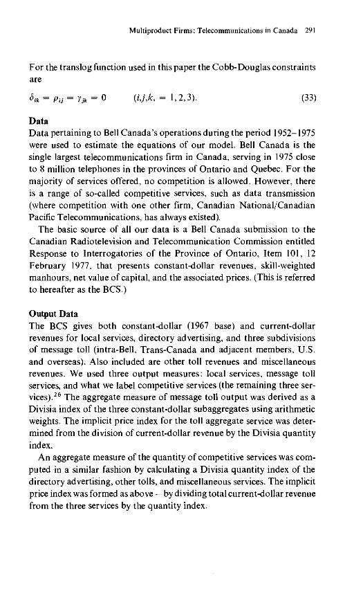
DataData pertaining to Bell Canada's operations during the period 1952-1975were used to estimate the equations of our model. Bell Canada is thesingle largest telecommunications firm in Canada, serving in 1975 closeto 8 million telephones in the provinces of Ontario and Quebec. For themajority of services offered, no competition is allowed. However, thereis a range of so-called competitive services, such as data transmission(where competition with one other firm, Canadian National/CanadianPacific Telecommunications, has always existed).
The basic source of all our data is a Bell Canada submission to theCanadian Radiotelevision and Telecommunication Commission entitledResponse to Interrogatories of the Province of Ontario, Item 101, 12February 1977, that presents constant-dollar revenues, skill-weightedmanhours, net value of capital, and the associated prices. (This is referredto hereafter as the BCS.)
Output DataThe BCS gives both constant-dollar (1967 base) and current-dollarrevenues for local services, directory advertising, and three subdivisionsof message toll (intra-Bell, Trans-Canada and adjacent members, U.S.and overseas). Also included are other toll revenues and miscellaneousrevenues. We used three output measures: local services, message tollservices, and what we label competitive services (the remaining three ser-vices).26 The aggregate measure of message toll output was derived as aDivisia index of the three constant-dollar subaggregates using arithmeticweights. The implicit price index for the toll aggregate service was deter-mined from the division of current-dollar revenue by the Divisia quantityindex.
An aggregate measure of the quantity of competitive services was com-puted in a similar fashion by calculating a Divisia quantity index of thedirectory advertising, other tolls, and miscellaneous services. The implicitprice index was formed as above—by dividing total current-dollar revenuefrom the three services by the quantity index.
Fuss and Waverman 292
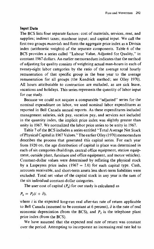
Input DataThe BCS lists four separate factors: cost of materials, services, rent, andsupplies; indirect taxes; manhour input; and capital input. We call thefirst two groups materials and form the aggregate price index as a Divisiaindex (arithmetic weights) of the separate components. Table 6 of theBCS provides a series called "Labour Value, Adjusted for Quality," inconstant 1967 dollars. An earlier memorandum indicates that the methodof adjusting for quality consists of weighting actual man-hours in each oftwenty-eight labor categories by the ratio of the average total hourlyremuneration of that specific group in the base year to the averageremuneration for all groups (the Kendrick method; see Olley 1970).All hours attributable to contruction are excluded, as are sick leave,vacations and holidays. This series represents the quantity of labor inputfor our study.
Because we could not acquire a comparable "adjusted" series for thenominal expenditure on labor, we used nominal labor expenditures asreported in Bell Canada annual reports. As these expenditures includedmanagement salaries, sick pay, vacation pay, and services not includedin the quantity index, the implicit price index was slightly greater thanunity in 1967. We normalized the labor price series to be unity in 1967.
Table 7 of the BCS includes a series entitled "Total Average Net Stockof Physical Capital in 1967 Values." The earlier Olley (1970) memorandumdescribes the process that generated this capital series. For each yearfrom 1920 on, the age distribution of capital in place was determined ineach of six categories (buildings, central office equipment, station equip-ment, outside plant, furniture and office equipment, and motor vehicles).Constant-dollar values were determined by reflating the physical stockby a Laspeyres price index (1967 = 1.0) for each capital type. Cash,accounts receivable, and short-term assets less short-term liabilities wereexcluded. Total net value of the capital stock in any year is the sum ofthe six individual constant-dollar categories.
The user cost of capital (Pk) for our study is calculated as
Pk = />,(/ + S),
where / is the expected long-run real after-tax rate of return applicableto Bell Canada (assumed to be constant at 6 percent), 5 is the rate of realeconomic depreciation (from the BCS), and Pt is the telephone plantprice index (from the BCS).
We have assumed that the expected real rate of return was constantover the period. Attempting to incorporate an increasing real rate led to
Multiproduct Firms: Telecommunications in Canada 293
implausible results. We chose 6 percent as the real rate, but also examinedthe effects of the alternative assumptions of 5 percent and 7 percent.Jenkins (1972, 1977) estimated the actual real after-tax rate of return fora wide cross-section of Canadian firms over the 1953-1973 period. Theaverage rate was 6 percent. For the communications sector, the 1965-1969average real rate was 5.2 percent including capital gains and 7 percentexcluding capital gains. For the 1965-1974 period Jenkins estimated theaverage rate, excluding capital gains, to be 7.2 percent for the communica-tions sector.
Empirical Results
Estimation ProcedureFor both the demand functions and the augmented-cost-equations systemthe method of estimation was iterative three-stage least squares, an asym-ptotically efficient simultaneous-equations procedure. The instrumentalvariables used for the right-hand-side endogenous variables were formedfrom the exogenous variables of the two systems: local service output,input prices, and real income.
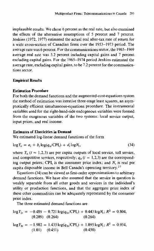
Estimates of Elasticities in DemandWe estimated log-linear demand functions of the form
logy;, = ax + MogC^/CPI,) + dt\ogNt, (34)
where Yit (i = 1,2,3) are per capita outputs of local service, toll service,and competitive services, respectively; qit (i = 1,2,3) are the correspond-ing output prices; CPI, is the consumer price index; and Nt is real percapita disposable income in Bell Canada's operating territory.27
Equations (34) can be viewed as first-order approximations to arbitrarydemand functions. We have also assumed that the service in question isweakly separable from all other goods and services in the individual'sutility or production functions, and that the aggregate price index ofthese other commodities can be adequately represented by the consumerprice index.
The three estimated demand functions are
lo gr l r = -0.489 - 0.721 logfaflr/CPIt) + 0.443\ogNt; R2 = 0.804,
(0.209) (0.264) (0.264)
log72( = -1.902 - 1.435 log(^2(/CPIt) + 1.095 logty; R2 = 0.934,(1.01) (0.451) (0.450)
Fuss and Waverman 294
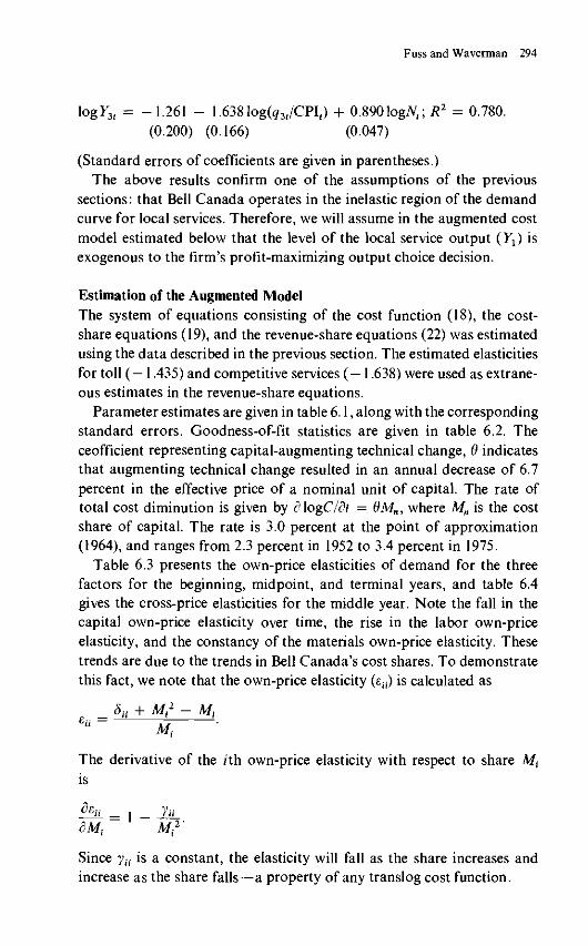
logF3f = -1.261 - 1.638log(q3t/CPlt) + 0.890logiV,; R2 = 0.780.(0.200) (0.166) (0.047)
(Standard errors of coefficients are given in parentheses.)The above results confirm one of the assumptions of the previous
sections: that Bell Canada operates in the inelastic region of the demandcurve for local services. Therefore, we will assume in the augmented costmodel estimated below that the level of the local service output (Yy) isexogenous to the firm's profit-maximizing output choice decision.
Estimation of the Augmented ModelThe system of equations consisting of the cost function (18), the cost-share equations (19), and the revenue-share equations (22) was estimatedusing the data described in the previous section. The estimated elasticitiesfor toll (— 1.435) and competitive services (—1.638) were used as extrane-ous estimates in the revenue-share equations.
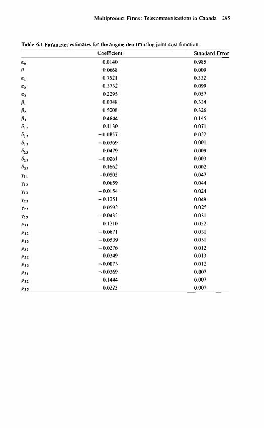
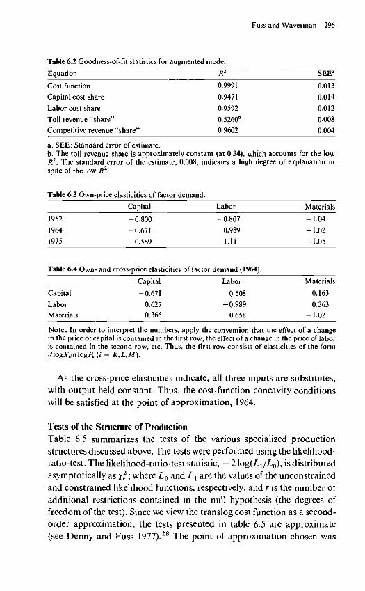
Parameter estimates are given in table 6.1, along with the correspondingstandard errors. Goodness-of-fit statistics are given in table 6.2. Theceofficient representing capital-augmenting technical change, 6 indicatesthat augmenting technical change resulted in an annual decrease of 6.7percent in the effective price of a nominal unit of capital. The rate oftotal cost diminution is given by d\ogC/dt = 9Mn, where Mn is the costshare of capital. The rate is 3.0 percent at the point of approximation(1964), and ranges from 2.3 percent in 1952 to 3.4 percent in 1975.
Table 6.3 presents the own-price elasticities of demand for the threefactors for the beginning, midpoint, and terminal years, and table 6.4gives the cross-price elasticities for the middle year. Note the fall in thecapital own-price elasticity over time, the rise in the labor own-priceelasticity, and the constancy of the materials own-price elasticity. Thesetrends are due to the trends in Bell Canada's cost shares. To demonstratethis fact, we note that the own-price elasticity (ea) is calculated as
_ 5it5it + M2 - Mt_
The derivative of the ith own-price elasticity with respect to share M{
is
fo = i V»M2'
Since yu is a constant, the elasticity will fall as the share increases andincrease as the share falls—a property of any translog cost function.
Multiproduct Firms: Telecommunications in Canada 295
Table 6.1 Parameter estimates for the augmented translog joint-cost function.
Coefficient Standard Error
a0
d
a2
a.
713
111
723
733
Pll
Pll
Pi 3
P21
P22
P23
P31
P32
P33
0.0140
0.0668
0.7521
0.3732
0.2295
0.0348
0.5008
0.4644
0.1130
-0.0857
-0.0369
0.0479
-0.0061
0.1662
-0.0505
0.0659
-0.0154
-0.1251
0.0592
-0.0435
0.1210
-0.0671
-0.0539
-0.0276
0.0349
-0.0073
-0.0369
0.1444
0.0225
0.985
0.009
0.332
0.099
0.057
0.334
0.326
0.145
0.071
0.022
0.001
0.009
0.003
0.002
0.047
0.044
0.024
0.049
0.025
0.031
0.052
0.051
0.031
0.012
0.013
0.012
0.007
0.007
0.007
Fuss and Waverman 296
Table 6.2 Goodness-of-fit statistics for augmented model.
Equation R2 SEEa
Cost function 0.9991 0.013
Capital cost share 0.9471 0.014
Labor cost share 0.9592 0.012
Toll revenue "share" 0.5260b 0.008
Competitive revenue "share" 0.9602 0.004
a. SEE: Standard error of estimate.b. The toll revenue share is approximately constant (at 0.34), which accounts for the lowR2. The standard error of the estimate, 0.008, indicates a high degree of explanation inspite of the low R2.
Table 6.3 Own-price elasticities of factor demand.
1952
1964
1975
Capital
-0.800
-0.671
-0.589
Labor
-0.807
-0.989
-1.11
Table 6.4 Own- and cross-price elasticities of factor demand (1964).
Capital
Labor
Materials
Capital
-0.671
0.627
0.365
Labor
0.508
-0.989
0.658
Materials
-1 .04
-1 .02
-1 .05
Materials
0.163
0.363
-1.02
Note: In order to interpret the numbers, apply the convention that the effect of a changein the price of capital is contained in the first row, the effect of a change in the price of laboris contained in the second row, etc. Thus, the first row consists of elasticities of the formd\ogXild\ogPk{i = K,L,M).
As the cross-price elasticities indicate, all three inputs are substitutes,with output held constant. Thus, the cost-function concavity conditionswill be satisfied at the point of approximation, 1964.
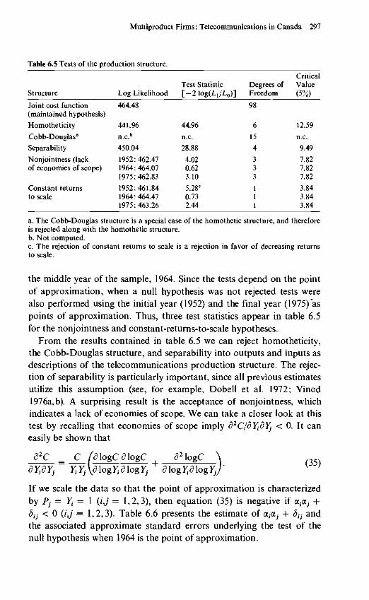
Tests of the Structure of ProductionTable 6.5 summarizes the tests of the various specialized productionstructures discussed above. The tests were performed using the likelihood-ratio-test. The likelihood-ratio-test statistic, —21og(L1/L0), is distributedasymptotically as Xr '•> where Lo and L1 are the values of the unconstrainedand constrained likelihood functions, respectively, and r is the number ofadditional restrictions contained in the null hypothesis (the degrees offreedom of the test). Since we view the translog cost function as a second-order approximation, the tests presented in table 6.5 are approximate(see Denny and Fuss 1977).28 The point of approximation chosen was
Multiproduct Firms: Telecommunications in Canada 297
Table 6.5 Tests of the production structure.
Structure
Joint cost function(maintained hypothesis)
Homotheticity
Cobb-Douglasa
Separability
Nonjointness (lackof economies of scope)
Constant returnsto scale
Log Likelihood
464.48
441.96
n.c.b
450.04
1952:462.471964:464.071975:462.83
1952:461.841964:464.471975:463.26
Test Statistic[-21og(L 1 /L 0 ) ]
44.96
n.c.
28.88
4.020.623.10
5.28C
0.732.44
Degrees ofFreedom
98
6
15
4
333
111
CriticalValue(5%)
12.59
n.c.
9.49
7.827.827.82
3.843.843.84
a. The Cobb-Douglas structure is a special case of the homothetic structure, and thereforeis rejected along with the homothetic structure.b. Not computed.c. The rejection of constant returns to scale is a rejection in favor of decreasing returnsto scale.
the middle year of the sample, 1964. Since the tests depend on the pointof approximation, when a null hypothesis was not rejected tests werealso performed using the initial year (1952) and the final year (1975) aspoints of approximation. Thus, three test statistics appear in table 6.5for the nonjointness and constant-returns-to-scale hypotheses.
From the results contained in table 6.5 we can reject homotheticity,the Cobb-Douglas structure, and separability into outputs and inputs asdescriptions of the telecommunications production structure. The rejec-tion of separability is particularly important, since all previous estimatesutilize this assumption (see, for example, Dobell et al. 1972; Vinod1976a, b). A surprising result is the acceptance of nonjointness, whichindicates a lack of economies of scope. We can take a closer look at thistest by recalling that economies of scope imply d2CldYidYi < 0. It caneasily be shown that
82C _ C fdlogCdlogCYt Yj \d log Yt d log Yj d log log Yj
(35)
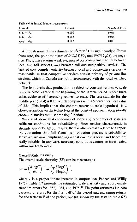
If we scale the data so that the point of approximation is characterizedby Pj = Y{ — 1 (i,j = 1,2,3), then equation (35) is negative if a ^ +3^ < 0 (ij = 1,2,3). Table 6.6 presents the estimate of a,aj + <5£j- andthe associated approximate standard errors underlying the test of thenull hypothesis when 1964 is the point of approximation.
Fuss and Waverman 298
Table 6.6 Estimated jointness parameters.
Formula
a t a 2 + 5l2
a1cc3 + <513
a2a3 + <523
Estimate
-0.016
0.002
-0.002
Standard Error
0.021
0.009
0.003
Although none of the estimates of d1C\dYidYi is significantly differentfrom zero, the point estimates of d2C/dY1dY2 and d2C/dY2dY3 are nega-tive. Thus, there is some weak evidence of cost complementarities betweenlocal and toll services, and between toll and competitive services. Thelack of cost complementarity between local and competitive services isreasonable, in that competitive services consist primary of private lineservices, which in Canada are not interconnected with the local switchednetwork.
The hypothesis that production is subject to constant returns to scaleis not rejected, except at the beginning of the sample period, where thereexists evidence of decreasing returns to scale. The test statistic for themiddle year (1964) is 0.13, which compares with a 5 percent critical valueof 3.84. This implies that the contant-returns-to-scale hypothesis is aclose description on the technology at the point of approximation usuallychosen in studies that use translog functions.
We stated above that economies of scope and economies of scale aresufficient conditions for subadditivity. Since neither characteristic isstrongly supported by our results, there is also no real evidence to supportthe contention that Bell Canada's production process is subadditive.However, we must emphasize again that our test is local, and hence notreally suitable. In any case, necessary conditions cannot be investigatedwithin our framework.
Overall Scale ElasticityThe overall scale elasticity (SE) can be measured as
dl
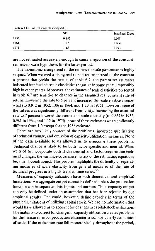
where X is a proportionate increase in outputs (see Panzer and Willig1975). Table 6.7 presents the estimated scale elasticity and approximatestandard errors for 1952, 1964, and 1975.29 The point estimates indicatedecreasing returns for the first half of the period and increasing returnsfor the latter half of the period, but (as shown by the tests in table 6.5)
Multiproduct Firms: Telecommunications in Canada 299
Table 6.7 Estimated scale elasticity (SE).
1952
1964
1975
SE
0.845
1.02
1.15
Standard Error
0.068
0.064
0.093
are not estimated accurately enough to cause a rejection of the constant-returns-to-scale hypothesis for the latter period.
The monotonic rising trend in the returns-to-scale parameter is highlysuspect. When we used a rising real rate of return instead of the constant6 percent that yields the results of table 6.7, the parameter estimatesindicated implausible scale elasticities (negative in some years, impossiblyhigh in other years). Moreover, the estimates of scale elasticities presentedin table 6.7 are sensitive to changes in the assumed real constant rate ofreturn. Lowering the rate to 5 percent increased the scale elasticity some-what (to 0.912 in 1952, 1.06 in 1964, and 1.20 in 1975); however, none ofthe values was significantly different from unity. Increasing the assumedrate to 7 percent lowered the estimate of scale elasticity (to 0.867 in 1952,0.981 in 1964, and 1.12 in 1975); none of these estimates was significantlydifferent from 1.0 except for the 1952 estimate.
There are two likely sources of the problems: incorrect specificationof technical change, and omission of capacity-utilization measures. Noneof the data available to us allowed us to overcome these problems.Technical change is likely to be both factor-specific and neutral. Whenwe tried to incorporate both Hicks neutral and factor-augmenting tech-nical changes, the variance-covariance matrix of the estimating equationsbecame ill-conditioned. This problem highlights the difficulty of separat-ing measures of scale elasticity from general measures of the rate oftechnical progress in a highly trended time series.30
Measures of capacity utilization have both theoretical and empiricallimitations. An aggregate output cannot be defined unless the productionfunction can be separated into inputs and outputs. Thus, capacity outputcan only be defined under an assumption that has been rejected by ourempirical results. One could, however, define capacity in terms of thephysical limitations of utilizing capital stock. We had no information thatwould have allowed us to account for changes in capital-stock utilization.The inability to correct for changes in capacity utilization creates problemsfor the measurement of production characteristics, particularly economiesof scale. If the utilization rate fell monotonically throughout the period,
Fuss and Waverman 300
perhaps because of capital expansion involving lumpy expenditures onincreasingly larger units, the inability to account for capacity utilizationwould bias the measure of scale elasticity upward.
The omission of some sources of technical change could also incorrectlyattribute to scale expansions in output that should be attributable tochanges in technology. Even with these two problems, which we feel biasthe estimates of scale elasticity upward in the latter part of the sampleperiod, no statistically significant economies of scale were found.
Incremental Costs and Their Relationships to Output PricesIncremental cost curves for each of the three output can be estimatedusing equation (25). With the midsample (1964) observations taken as thefixed values of input prices and irrelevant outputs, the incremental costcurves were found to be downward-sloping for all three outputs.31
Since the incremental cost elasticities are increasing for all three outputs(c2 logC/d log Yf = 5n > 0), at some output level incremental costs mustincrease. For all three services the regions of increasing incremental costsoccur at output levels greater than that observed in the sample. Wearbitrarily doubled each of the three outputs, and reestimated the incre-mental cost elasticities assuming that the observed relationship betweenoutput and costs still held. Marginal-cost curves continued to fall atthese higher outputs.
We do not find it very useful to compare incremental costs with pricescharged for these services for the purposes of examining relative contri-butions and "cream-skimming" as usually defined in regulatory hearings.As we indicated previously, these incremental costs are based on replace-ment or opportunity cost concepts, while the firm is regulated on ahistorical capital cost basis. Prices could then be below these incrementalopportunity costs but be above historical fully allocated average costsas determined in regulatory hearings. Valuing inputs at opportunity costs(replacement value) might indicate losses when compared with actualrevenue even though the firm was earning its allowed rate of return onits rate base. In our study, only the cost of capital and the value of thecapital input exhibit differences between historical and opportunity costs.Though the firm has to pay each unit of labor the opportunity cost ineach year, regulators do not allow the firm to revalue its capital (or ratebase) every year on the basis of replacement value and the opportunitycost of capital.
However, it is of some interest to compare output price with incremental

Multiproduct Firms: Telecommunications in Canada 301
Table 6.8 Actual prices and incremental costs (replacement value).
1952
1964
1975
Local Services
Price
0.92
1.00
1.18
Note: The index is 1967a. Incremental cost.
ICa
2.16
1.73
1.48
- 1.0.
Toll Services
Price
1.05
1.04
1.19
IC
0.40
0.34
0.22
Competitive Services
Price
0.78
1.00
1.56
IC
0.32
0.41
0.30
cost for the purposes of evaluating the efficiency aspects of rate setting.Table 6.8 compares prices and marginal costs, where the opportunitycost of capital used in the calculations is the nominal after-tax realizedrate of return.
In all years of the sample, the actual price for local service was belowthe measured incremental replacement cost for that service. In all years,the actual prices for both toll and competitive services were substantiallyabove the marginal costs of these respective services. If there were indeedno economies of scale, marginal-cost pricing would cover all costs. Pricingat the marginal costs of the services would substantially lower the pricesfor toll and competitive services and increase the price of local service. Ifthere were increasing returns to scale, marginal-cost pricing could notcover all costs. We cannot calculate the second-best set of Ramsey prices,constraining the firm to break even, since one of the three services wasestimated to have a constant elasticity of demand less than unity implynegative marginal revenue.32
Sensitivity of the Empirical Results to Alternative Elasticity AssumptionsThe extraneous demand elasticities are estimated from rather ad hocspecifications. We therefore investigated the sensitivity of all our empiricalresults to alternative estimates of demand elasticities. We increased theabsolute value of the point estimates of toll-service and competitive-service demand elasticities by two standard deviations. The adjusteddemand elasticities are —2.30 for toll service and —2.03 for competitiveservices. The parameter estimates did change, but the characteristics ofproduction did not change in any significant way. The estimates of thescale elasticity fell marginally (0.98 in 1964 as compared with 1.02 withthe lower demand elasticities; 1.10 in 1975 as compared with 1.14 for ourbase-case results).
Fuss and Waverman 302
The Behavior of the Multiproduct Firm Subject to Rate-of-ReturnRegulation—A Duality Approach
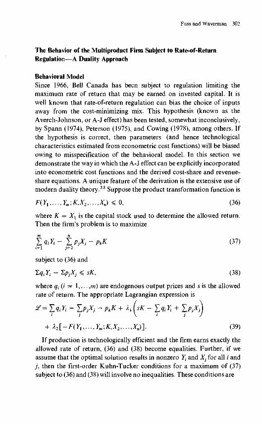
Behavioral ModelSince 1966, Bell Canada has been subject to regulation limiting themaximum rate of return that may be earned on invested capital. It iswell known that rate-of-return regulation can bias the choice of inputsaway from the cost-minimizing mix. This hypothesis (known as theAverch-Johnson, or A-J effect) has been tested, somewhat inconclusively,by Spann (1974), Peterson (1975), and Cowing (1978), among others. Ifthe hypothesis is correct, then parameters (and hence technologicalcharacteristics estimated from econometric cost functions) will be biasedowing to misspecification of the behavioral model. In this section wedemonstrate the way in which the A-J effect can be explicitly incorporatedinto econometric cost functions and the derived cost-share and revenue-share equations. A unique feature of the derivation is the extensive use ofmodern duality theory.33 Suppose the product transformation function is
F(Y1,...,Ym,K,X2,...,Xn) <0, (36)
where K = X1 is the capital stock used to determine the allowed return.Then the firm's problem is to maximize
Y^ ^jj (37)
subject to (36) and
T,qiYt - ZpjXj <sK, (38)
where qt(i = 1,... ,m) are endogenous output prices and s is the allowedrate of return. The appropriate Lagrangian expression is
j - PkK + X, (sK - lqiYt
+ X2\_-F(Y1,...,Ym,K,X2,...,Xn)l (39)
If production is technologically efficient and the firm earns exactly theallowed rate of return, (36) and (38) become equalities. Further, if weassume that the optimal solution results in nonzero Yt and X-} for all / andj , then the first-order Kuhn-Tucker conditions for a maximum of (37)subject to (36) and (38) will involve no inequalities. These conditions are

Multiproduct Firms: Telecommunications in Canada 303
<40)
and
~ X,§ = 0, (41)
ldYt
or (42)
where MR, is the marginal revenue of the /th output.Differentiating (39) with respect to Xx and X2 gives
= sK - YqJi - YpjX: = 0 (43)
and
^ = -F(Y1,...,Ym,K,X2,...,Xn) = 0. (44)
From (40) and (41) we obtain
"" ^ = 4 (g,l=l,...,n), (45)
....( 4 6 )
and
BF IBF p , ( l -A. ) p*
where /?*, /?*, and /?* are shadow prices of the inputs. Equations (45) and(46) state that in the optimal solution the firm sets the marginal rate oftechnical substitution equal to the ratio of shadow prices. But this con-dition is just the usual cost-minimization condition, except for the factthat the prices are shadow prices instead of market prices. The firm canbe viewed as acting as if it minimized cost subject to the shadow prices.Therefore, by solving equations (43)-(46) we can obtain the producer'sconstrained multiproduct cost function,
C* = C*(p*l,...,p*,Ylt...,YJ. (47)
Fuss and Waverman 304
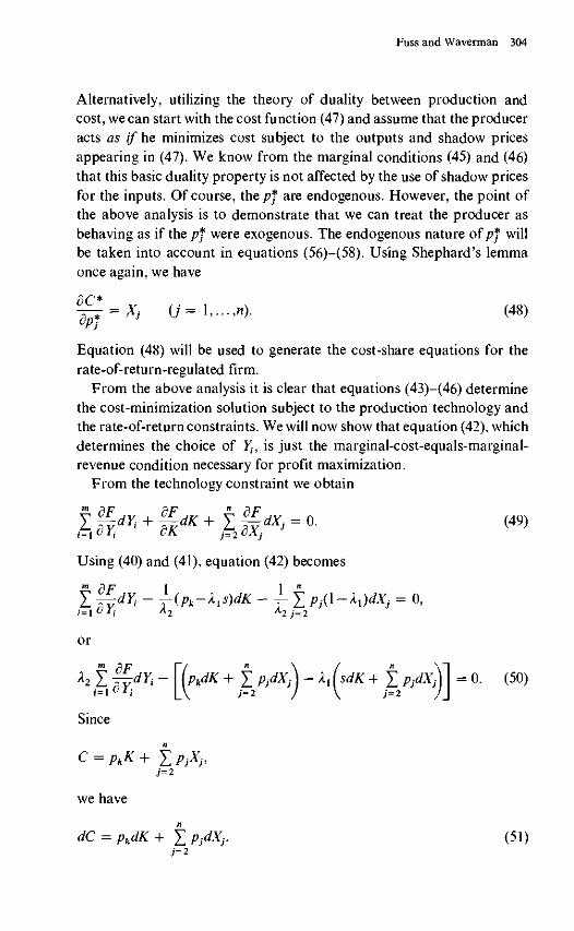
Alternatively, utilizing the theory of duality between production andcost, we can start with the cost function (47) and assume that the produceracts as if he minimizes cost subject to the outputs and shadow pricesappearing in (47). We know from the marginal conditions (45) and (46)that this basic duality property is not affected by the use of shadow pricesfor the inputs. Of course, the p* are endogenous. However, the point ofthe above analysis is to demonstrate that we can treat the producer asbehaving as if the p* were exogenous. The endogenous nature of/?* willbe taken into account in equations (56)—(58). Using Shephard's lemmaonce again, we have
J ^ = XJ C / = l , • • . , « ) . ( 4 8 )
Equation (48) will be used to generate the cost-share equations for therate-of-return-regulated firm.
From the above analysis it is clear that equations (43)-(46) determinethe cost-minimization solution subject to the production technology andthe rate-of-return constraints. We will now show that equation (42), whichdetermines the choice of Yh is just the marginal-cost-equals-marginal-revenue condition necessary for profit maximization.
From the technology constraint we obtain
Using (40) and (41), equation (42) becomes
m f)F 1 1 "
£ T?dYi ~ T(Pk-^)dK - f I Pj(\ -XJdXj = 0,i=lCIi A2 A2j=2
or
X2 I jydYi - UdK + ^PjdXA - XxisdK + ZPjdXA = 0. (50)
Since
j=2
we have
dC = pkdK+ tpjdXj. (51)7=2

Multiproduct Firms: Telecommunications in Canada 305
In addition, from (43),
sdK + XpjdXj = d&qiYi) = dR. (52)
Now suppose that only Y, changes, so that dYk = 0(k # /). Then equation(50) becomes, using (51) and (52),
where
dR = d^qJi) (dYk = 0, k # /).
We can write equation (51) in the form
f r i ^ • <52'>Substituting for X1dFldYi in equation (42), we obtain
M R J C I - A J - [MC,—AtMRJ = 0,
or
MR,- = MQ. (53)
Thus, equation (42) is just the MR = MC condition in somewhatdisguised form.
The above interpretation of the first-order conditions suggests that theoverall optimization problem can be subdivided into two sequential prob-lems. First, for any outputs, minimize cost subject to the technologyand rate-of-return constraints. This defines the output expansion path interms of shadow-price tangency conditions from equations (40), (41), (43),and (44). Second, conditional on the optimal input proportions, chooseoutputs so as to equate marginal revenue to marginal cost (from equation(42)).
Because a sequential analysis can be applied in the case of rate-of-return regulation, the approach used in the earlier sections of this paperis relevant. That is, first use the cost function to obtain the input demandequations and then use the profit-maximizing conditions to determine theoptimal Yv.
The constrained cost function C* can be written as
C* = ptK + £ pfXp (54)j=2
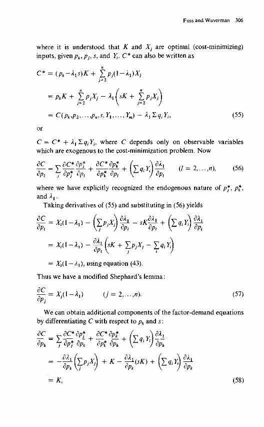
Fuss and Waverman 306
where it is understood that K and X} are optimal (cost-minimizing)inputs, given pk, pp s, and Yt. C* can also be written as
C* = (pk-XlS)K + j^Pjil-X^Xj7=2
JXJ - X, (sK + t Pjx)7=2
= C(pk,p2,...,pn,s,Yl,...,Ym) - kxJLqiYh (55)
or
C — C* + X^TqiYi, where C depends only on observable variableswhich are exogenous to the cost-minimization problem. Now
^ (l = 2,...,n), (56)
where we have explicitly recognized the endogenous nature of pf, p*,and Xx.
Taking derivatives of (55) and substituting in (56) yields
f- = X,0 -A,) - hpjx) ^ - SK3^ + hq,r) ^dPl \y JJ dPl dPl \^ ) 8Pl
= X,(l —/J , using equation (43).
Thus we have a modified Shephard's lemma:
^ j X , ) (j = 2,...,n). (57)
We can obtain additional components of the factor-demand equationsby differentiating C with respect to pk and s:
a c = ec^dpi d&dpt fy ^fa dpfdP dp*dP\Lqi {)dP
(58)
=
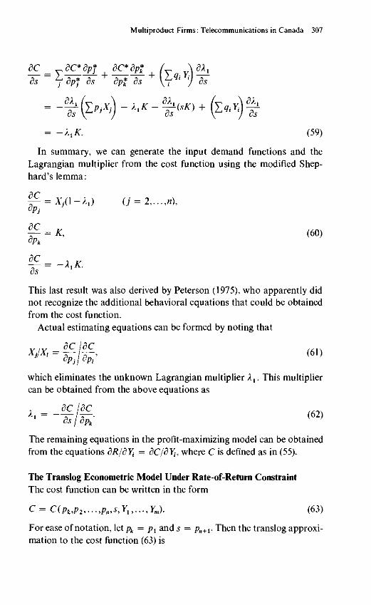
Multiproduct Firms: Telecommunications in Canada 307
l dC^djl f \dX^s dpt 8s \yqt l) ds
fds ydpj ds dpt 8s \yqt l) ds
= -X,K. (59)
In summary, we can generate the input demand functions and theLagrangian multiplier from the cost function using the modified Shep-hard's lemma:
1^ = ^.(1-^0 (j = 2,...,n),
— - -X Kds ~ 1 '
This last result was also derived by Peterson (1975), who apparently didnot recognize the additional behavioral equations that could be obtainedfrom the cost function.
Actual estimating equations can be formed by noting that
Y IV — / (f\\\il I — ^ / "\ ' V )
which eliminates the unknown Lagrangian multiplier Xl. This multipliercan be obtained from the above equations as
X\ = — ^ - hr- • (62)ds I dpk
The remaining equations in the profit-maximizing model can be obtainedfrom the equations dR/dYi = dC/dYt, where C is defined as in (55).
The Translog Econometric Model Under Rate-of-Return ConstraintThe cost function can be written in the form
C = C(pk,p2,...,pn,s,Yl,...,YJ. (63)
For ease of notation, let pk — p1 and s = pn+v Then the translog approxi-mation to the cost function (63) is

Fuss and Waverman 308
m n + 1
logC = a0 + aTT + X a, log 7, + £
m m
Z Ei = l f e = ln + 1 n + 1
+ i Z Z logPj
m n + 1
+ I Ipyiogy;-iog^. (64)
The cost-share equations become
d\ogC =pJ(l-ll)Xjd \ogpj
aiogcd log/7 i
SlogC
C
n + l
k = l
cf
n + 1
L + Z Tlfcioj
P n + 1 \ 1 ~^ 1 J
m
i = l
m
zpk + y~ r K ^^
i=i
1
(65)
Iftilogy,, (66)
i C
n + 1 m
= Pn+i + V yn + 1 fclogPk + Z P; n+il°g ;> (67)k= i ; = I
where Mn+1 = pn+1X1/C is the allowed rate-of-return "cost share."The cost system to be estimated consists of equations (64) and (66) and
equations of the form
(68)n + 1 m
+ Z y2kiogA + Z Ptf
Multiproduct Firms: Telecommunications in Canada 309
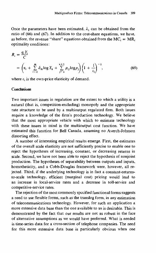
Once the parameters have been estimated, Xx can be obtained from theratio of (66) and (67). In addition to the cost-share equations, we have,as before, the revenue "share" equations obtained from the MC, = MR;
optimality conditions:
= a,- + X Sik\ogYk + X pylog^ 1 + - ) , (69)
where £t is the own-price elasticity of demand.
Conclusions
Two important issues in regulation are the extent to which a utility is anatural (that is, competition-excluding) monopoly and the appropriaterate structure to be used by a multioutput regulated firm. Both issuesrequire a knowledge of the firm's production technology. We believethat the most appropriate vehicle with which to estimate technologywith these issues in mind is the multioutput cost function. We haveestimated this function for Bell Canada, assuming no Averch-Johnsondistorting effect.
A number of interesting empirical results emerge. First, the estimatesof the overall scale elasticity are not sufficiently precise to enable one toreject the hypotheses of increasing, constant, or decreasing returns inscale. Second, we have not been able to reject the hypothesis of nonjointproduction. The hypotheses of separability between outputs and inputs,homotheticity, and a Cobb-Douglas framework were, however, all re-jected. Third, if the underlying technology is in fact a constant-returns-to-scale technology, efficient (marginal cost) pricing would lead toan increase in local-service rates and a decrease in toll-service andcompetitive-service rates.
The rejection of the most commonly specified functional forms suggestsa need to use flexible forms, such as the translog form, in any estimationof telecommunications technology. However, for such an application amore extensive data base than the one available to us is desirable. This isdemonstrated by the fact that our results are not as robust in the faceof alternative assumptions as we would have preferred. What is neededis time-series data for a cross-section of telephone companies. The needfor this more extensive data base is particularly obvious when one

Fuss and Waverman 310
contemplates the estimation of the multioutput cost-function modelwhich takes into account Averch-Johnson effects.
We thank the University of Toronto Institute for Policy Analysis for providing computerfunds, and Angelo Molino for excellent research assistance.
Notes
1. For attempts to define multiproduct scale economies see Baumol and Braunstein 1977,Baumol 1977, and Panzar and Willig 1978.
2. For an application of multiproduct cost functions to U.S. railroad data see Brownetal. 1976.
3. This proof is taken from Brown et al. 1976, p. 9.
4. We are ignoring for the moment the problems of defining economies of scale, of measuringoutput for a firm producing a number of products, and of defining average cost.
5. Baumol et al. (1976) and Baumol and Braunstein (1977) refer to this change as "economiesof scope," such as the economies of integrating a number of products within a firm.
6. They only help since the benefits of a single firm must be compared to the benefits ofcompetition, product diversity, innovation, and cost minimization.
7. In the case of a single output, m = 1 and equation (1) can be solved explicitly as Yx =f(X1,... ,Xn), which is the usual form of the production function.
8. For an introduction to duality theory and the use of Shephard's lemma see Baumol1977a, chap. 14.
9. If production is not joint, then
C(YU.. . ,7m;JP1 , . . . ,Pn) = £ C'(Yt,Plf.. . ,Pn)i=l
(see Hall 1973). In this case the multiple-output technology is just a collection of single-outputtechnologies, and
dlogC _ dlogC"'<91ogF, "~ dlogy,-
is an unambiguous measure of returns to scale.
10. Panzar and Willig (1978) developed a measure of product-specified economies of scalewhich may provide a solution to the consistency problem. However, their measure requiresknowledge of the cost function in the region where one or more outputs are zero, andsuch output levels are generally unobservable.
11. See Kahn 1970, p. 53; FCC docket 20003 (Cost Separation); FCC docket 18128(Telepek); FCC Docket 19919; Canadian Transport Commission "Cost Inquiry."
12. We are indebted to M. A. Schankerman for a memorandum entitled "Contributionsand Cream-Skimming in Telecommunications Services."
13. The FCC in 1967 allocated the costs of local loops and switches to inter- and intrastateservice by their relative minutes of use. When this formula resulted in "too low" a figurefor interstate use, it was multiplied by three to reflect the higher "value" of interstateservice (Kahn 1970, p. 153). Actually, to utilize demand elasiticities to determine the
Multiproduct Firms: Telecommunications in Canada 311
"opportunity costs" of various joint services may be correct. However, demand studiesindicate that the demand for interstate service is more elastic than that for intrastate service.Efficient pricing rules would suggest a relative decrease in the price for interstate service.
14. Economies of fill are not related in any way to long-run economies of scale.
15. In the above example, econometric analysis could associate the upgrading changes incost with the data users if residential voice traffic did not increase at the same time. However,were business and residential traffic to increase by the same amount, system-upgradingcosts would be associated with both types of demand. The typical time-series data used instudies of the telecommunications sector, including data available to us, are too highlyaggregated and time-trended to permit these causal types of relationships to be estimatedwith any degree of precision. The required information would be time-series, cross-sectionaldata for a number of telephone companies.
16. One cannot use some historical embedded average cost of capital in econometricanalysis, since the firm does not face these average embedded costs at the margin. Maximizingprofits dependent on these embedded costs would yield the incorrect factor proportionsand output decisions based on actual current market prices.
17. See Dobell et al. 1972; Waverman 1977; Houthakker and Taylor 1970.
18. This result is correct as long as demand complementarities among the monopolist'sproducts are not sufficiently strong that an increase in the price of the product with inelasticdemand so reduces demand for other products that the monopolist's total revenue falls.
19. See note 18 for an applicable qualification.
20. In the case of substitutability or complementarity among the monopolist's products,marginal revenue would be given by
Since our empirical demand functions did not indicate the existence of the required inter-relationships, this more general case has been relegated to a note.
21. In the actual estimation, the stability conditions
dY < dYi
were satisfied at all data points.
22. We attempted to incorporate Hicks's neutral technical change both instead of and inaddition to capital-augmenting technical change. The attempts proved unsuccessful.
23. It can be shown that if demand interdependence is present,
d logy;. <
where e,; is the cross-price elasticity of demand for product 7, with respect to price q^.
24. Since C is based on opportunity or replacement cost while the firm's actual revenueis constrainted by historical cost, £/?,- can be less than C with the firm still earning itsallowed rate of return. '
25. See Denny and Pinto 1978. A more detailed description of this test is provided below.
26. The three subcategories contained in the aggregate "competitive" service are othertoll (private line, data communications, broadband, TWX); miscellaneous (consulting andother services), and directory advertising. Directory advertising was spun off to form a
Fuss and Waverman 312
separate company at the end of 1971. Our estimation procedure took this exogenous shiftin revenues into account.
27. Although we attempted other formulations incorporating cross-elasticity effects, noneof these attempts proved successful. There was no indication of significant interdependenceamong the demands for the three services.
28. The tests for homotheticity and the Cobb-Douglas structure are also exact in the sensethat they do not depend on the point of approximation.
29. Standard errors were calculated as linear approximations. See Kmenta 1971, p. 444.
30. The measures of cost-diminution technical change and returns to scale are both mono-tonically trended. However, their combined effect on total factor productivity is to producean almost constant rate. Ohta (1974) showed that the rate of total factor productivity canbe measured as Ef^1 • sCt, where eCY is the scale elasticity and £ o is the rate of total costdiminution. The resulting rates of total factor productivity are 2.7 percent in 1952, 2.9percent in 1964, and 3 percent in 1975.
31. We reemphasize that a falling incremental cost curve is not necessarily associated withoverall increasing returns to scale.
32. Only if an even number of services were subject to inelastic demands would we beable to calculate a Ramsey price vector. The solution, of course, is to relax the assumptionof constant demand elasticities so that increasing the price of local services will eventuallyplace the product in an estimated elastic demand region.
33. The approach taken in this section is similar to that used by Cowing (1978). However,we make more explicit use of duality theory to obtain the estimating equations, and donot need to assume profit-maximizing behavior with respect to the production of all outputs.
References
Baumol, W. J. 1977a. Economic Theory and Operations Analysis, fourth edition. EnglewoodCliffs, N.J.: Prentice-Hall.
. 1977b. "On the Proper Cost Tests for Natural Monopoly in a Multiproduct In-dustry." American Economic Review 67: 809-822.
Baumol, W. J., and Braunstein, Y. M. 1977. "Empirical Study of Scale Economies andProduction Complementarity: The Case of Journal Publication." Journal of PoliticalEconomy 85: 1037-1048.
Baumol, W. J., Bailey, E. E., and Willig, R. D. 1977. "Weak Invisible Hand Theorems onthe Sustainability of Prices in a Multiproduct Monopoly." American Economic Review67:350-365.
Berndt, E. R., and Wood, D. W. 1975. "Technology, Prices and Derived Demand forEnergy." Review of Economics and Statistics 57: 259-268.
Brown, R., Caves, D., and Christensen, L. 1976. Estimating Marginal Costs for Multi-Product Regulated Firms. Social Systems Research Institute working paper 7609, Universityof Wisconsin, Madison.
Cowing, T. 1978. "The Effectiveness of Rate-of-Return Regulation: An Empirical Testusing Profit Functions." In M. Fuss and D. McFadden (eds.), Production Economics: ADual Approach to Theory and Applications. Amsterdam: North-Holland.
Denny, M., and Fuss, M. 1977. "The Use of Approximation Analysis to Test for Separabilityand the Existence of Consistent Aggregates." American Economic Review 67: 404-418.
Multiproduct Firms: Telecommunications in Canada 313
Denny, M., and Pinto, C. 1978. "An Aggregate Model with Multi-Product Technologies."In M. Fuss and D. McFadden (eds.), Production Economics: A Dual Approach to Theoryand Applications. Amsterdam: North-Holland.
Diewert, W. E. 1971. "An Application of the Shephard Duality Theorem: A GeneralizedLeontief Production Function." Journal of Political Economy 79: 481-507.
Dobell, A. R., Taylor, L. D., Waverman, L., Liu, T. H., and Copeland, M. D. G. 1972."Communications in Canada." Bell Journal of Economics and Management Science 3:179-219.
Fuss, M. A. 1977. "The Demand for Energy in Canadian Manufacturing: An Exampleof the Estimation of Production Structures with Many Inputs." Journal of Econometrics5:89-116.
Hall, R. E. 1973. "The Specification of Technologies with Several Kinds of Outputs."Journal of Political Economy 81: 878-892.
Houthakker, H. S., and Taylor, L. D. 1970. Consumer Demand in the United States. 2ndedition. Cambridge, Mass.: Harvard University Press.
Jenkins, G. P. 1972. Analysis of Rates of Return from Capital in Canada. PhD. diss.,Dept. of Economics, University of Chicago.
. 1977. Capital in Canada: Its Social and Private Performance 1965-1974. Economic
Council of Canada discussion paper 98.
Kahn, A. E. 1970, 1971. The Economics of Regulation. 2 vols. New York: Wiley.
Kmenta, J. 1971. Elements of Econometrics. New York: Macmillan.Lau, L. J. 1978. "Applications of Profit Functions." In M. Fuss and D. McFadden (eds.),Production Economics: A Dual Approach to Theory and Applications. Amsterdam: North-Holland.
Ohta, M. 1974. "A Note on the Duality between Production and Cost Functions: Rate ofReturn to Scale and Rate of Technical Progress." Economic Studies Quarterly 25: 63-65.
Olley, R. E. 1970. Productivity Gains in a Public Utility—Bell Canada 1952 to 1967. Paperpresented at the annual meeting of the Canadian Economics Association.
Panzar, J. C , and Willig, R. D. 1975. Economics of Scale and Economies of Scope inMulti-Output Production. Bell Laboratories discussion paper 33.
. 1979. Economies of Scope, Product Specific Economies of Scale, and the Multi-product Competitive Firm. Bell Laboratories economics discussion paper 152.
Peterson, H. C. 1975. "An Empirical Test of Regulatory Effects." Bell Journal of Economics6:111-126.
Spann, R. 1974. "Rate of Return Regulation and Efficiency in Production: An EmpiricalTest of the Averch-Johnson Thesis." Bell Journal of Economics and Management Science5: 38-52.
Vinod, H. D. 1976a. "Application of New Ridge Regression Methods to a Study of BellSystem Scale Economies." Journal of the American Statistical Association 71: 929-933.
. 1976b. Bell Scale Economies and Estimation of Joint Production Functions. BellLaboratories, Holmdel, N.J. Submitted in the Fifth Supplemental Response, FCC docket20003.
Waverman, L. The Demand for Telephone Services in Britain. Mimeographed. Universityof Toronto Institute for Policy Analysis.
Comment
Ronald Braeutigam
The article by Fuss and Waverman represents a major step forward inempirical research in the telephone industry. Their study generates anumber of interesting conclusions, but even more important is the factthat it applies solid theoretical and empirical techniques to a difficultproblem. The use of a flexible-form cost function and the theory ofduality enables the authors to test a number of propositions which earlierstudies have employed as maintained hypotheses. In addition, the eco-nometric methods used in the paper are novel applications of well-knowntechniques, generally well justified, and help to identify areas wherefuture research may lead to an even better understanding of the underlyingtechnology.
Among the most interesting empirical results are the following. Theauthors cannot reject the null hypothesis that there are constant returnsto scale in the industry. Neither can they reject the null hypothesis thatthere are no economies of scope. They do reject the proposition thatthe production function is homothetic, as well as the separability ofinputs and outputs. The authors have also integrated a technical-changecoefficient in their analysis, and conclude that capital-augmented technicalchange helped to reduce total cost at an annual rate of about 3 percentover the period 1952-1975. Finally, they have produced estimates ofmarginal cost for three types of services: local service, message toll, and"competitive" services (private line, broadband, and TWX). They suggestthat local-service tariffs have been less than marginal cost for the period1952-1975, while the tariffs for the other two service categories haveexceeded marginal costs. They conclude that more efficient pricing wouldtherefore result from some increase in local-service tariffs and somedecrease in the other tariffs.
The techniques and the conclusions both represent important contri-butions to our understanding of the technology of telecommunications.Additionally, they provoke the reader to ask a number of questionswhich it may now be possible to answer with the advances in techniquethat are used in the article.
Comment on Fuss and Waverman 315
Usefulness of Cost Data
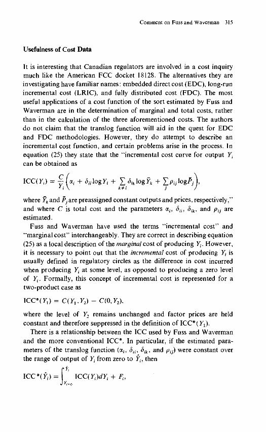
It is interesting that Canadian regulators are involved in a cost inquirymuch like the American FCC docket 18128. The alternatives they areinvestigating have familiar names: embedded direct cost (EDC), long-runincremental cost (LRIC), and fully distributed cost (FDC). The mostuseful applications of a cost function of the sort estimated by Fuss andWaverman are in the determination of marginal and total costs, ratherthan in the calculation of the three aforementioned costs. The authorsdo not claim that the translog function will aid in the quest for EDCand FDC methodologies. However, they do attempt to describe anincremental cost function, and certain problems arise in the process. Inequation (25) they state that the "incremental cost curve for output Yt
can be obtained as
lCC(Yt) = ~U + ^logF; + X <5lfclogfk + ZPI i \ k±i j
where Yk and P-} are preassigned constant outputs and prices, respectively,"and where C is total cost and the parameters a;, Sih Sik, and pu areestimated.
Fuss and Waverman have used the terms "incremental cost" and"marginal cost" interchangeably. They are correct in describing equation(25) as a local description of the marginal cost of producing Y{. However,it is necessary to point out that the incremental cost of producing Y{ isusually defined in regulatory circles as the difference in cost incurredwhen producing Y, at some level, as opposed to producing a zero levelof Y{. Formally, this concept of incremental cost is represented for atwo-product case as
ICC*^) = C(YltY2) - C(0,Y2),
where the level of Y2 remains unchanged and factor prices are heldconstant and therefore suppressed in the definition of ICC* (Yx).
There is a relationship between the ICC used by Fuss and Wavermanand the more conventional ICC*. In particular, if the estimated para-meters of the translog function (a,, du, dik, and ptj) were constant overthe range of output of Y, from zero to Yh then
ICC*(y/) - lCCiYJdYt + Ft,

Braeutigam 316
where, in addition to the variables already defined, Ft represents a fixedcost that is not incurred unless Y{ is positive.
The distinction between ICC*(T;) and ICC(Yj) emphasizes two majorpoints about the translog function. First, since it is a Taylor-seriesapproximation of a function, it will generally be accurate only locally. Theparameters a,, <)„, Sik, and ptj will generally not be constant as Yt variesfrom zero to Yt. Second, the translog function cannot accommodate azero as one of its arguments (in particular, Yi = 0), since it involves alogarithm of zero. Moreover, if avoidable fixed costs are attributable toa service (such as Ft in the example above), the cost function is not con-tinuous at Yi — 0. If it is not continuous, then neither is it differentiableat Yt = 0.
Fuss and Waverman are aware of these limitations. They note thatthe local nature of the estimation prohibits their testing for subadditivityin the cost function. Our purpose here is simply to point out why onewill not be able to infer the usual kind of incremental cost informationreferred to by regulators—ICC*—from the estimated cost function.
Joint Production and Economies of Scope
One part of the article that may cause some confusion is the treatmentof "joint production." The authors describe joint production as meaningthat the production function can be written as (equation (3))
,,...,Xn) = mm(a1Y1,a2Y2,...,amYm),
but cannot be written as (equation (2))
*m = Fm(Xh+ i, . . . ,Xn),
where the Y variables refer to output levels and the X variables to inputlevels. In other words, the authors are characterizing a joint productionprocess as one in which each input cannot be uniquely attributed to theproduction of a particular output.
The first point needing clarification involves the statement that "eco-nomies of scope exist if and only if production is joint." Economies ofscope may exist in some cases without joint production; thus the "only if"part of the statement does not appear to be true. For example, considerthe following cost function:
Comment on Fuss and Waverman 317
C = 10 + Y, + Y2.
Note that the process involves costs which cannot all be attributed un-ambiguously to individual outputs, but production is not joint. However,also note that
C(4,5) = 19,
C(0,5) = 15,
C(4,0) = 14.
Thus,
C(4,5) < C(0,5) + C(4,0),
and the cost function does exhibit economies of scope, even thoughproduction is not joint.
The second point involves the statement that "economies of scopeimply d2C/dYjdYj < 0." The implication is not generally true of costfunctions. For example, consider the cost function
C = F + Yx + Y2,
where F is a fixed, shared cost. Then
C{YUY2) = F+ Y,+ Y2< C(0,F2) + C(Ylt0) = IF + Yt + Y2
and there are economies of scope, even though d2C/8Y1dY2 •£ 0.
Model Specification
At the heart of the article is an estimation of a translog cost function. Thetheoretical basis for the work is presented clearly. Specifically, it isassumed that the firm minimizes total cost in producing any observedvector of output, with no effect to the contrary such as an Averch-Johnsonbias. The importance of this assumption is recognized explicitly by theauthors, and a theoretical discussion of the A-J variation is presented inthe concluding section. With this in mind, we confine our comments tothe cost-minimizing model estimated in the article.
Those who have worked with translog cost functions are no doubtfamiliar with the property that the number of parameters to be estimatedincreases rapidly as the number of outputs and factor prices increases.Some aggregation is needed to make the model tractable. For example,the thought of having a translog function that includes factor prices for
Braeutigam 318
each of the twenty-eight types of labor mentioned in the paper bogglesthe mind! While one might like to see how the empirical results areaffected by, for example, using four or five outputs instead of three, theauthors are constrained by the amount of data they have available. Inlight of this, the categories of outputs chosen seem reasonable.
We address two areas of specification here. The first involves the fol-lowing statement:
For observed output levels such that demand is elastic, we assumethat marginal revenue is set equal to marginal cost. For output levelssuch that demand is inelastic, we assume that those outputs areexogenous to the firm.
In other words, Fuss and Waverman have run a set of separate regressionsto determine the demand schedules for each of the three output categoriesselected, and then calculated an elasticity of demand for each. They findthat local service had an inelastic demand, and conclude that price (orquantity) regulation has in effect made the level of local service exogenousto the firm.
They find the other two service categories to have elastic demands,and therefore conclude that these output levels are endogenous to thefirm, determined by profit-maximizing behavior (setting the marginalrevenue equal to the marginal cost) in each market. There exists theuncomfortable possibility that regulators have specified the price (orquantity) level in each market at a level such that marginal cost exceedsmarginal revenue, where the marginal revenue remains positive. Restated,the observation of a nonnegative marginal revenue is a necessary, butnot sufficient condition for the profit-maximizing behavior assumed bythe authors. (This assumes that the outputs are not complements; theissue of cross elasticities of demand will be addressed below.) Fuss andWaverman could have reinforced the validity of their endogeneity assump-tions in these two markets with some additional institutional descriptionabout the way in which the regulatory process does in fact work.
A second potential problem of specification arises from the estimationof the log-linear demand functions used to provide additional informa-tion for the estimation of the cost function itself. Fuss and Wavermanhave assumed that each service "is weakly separable from all other goodsand services in the individual's utility or production functions, and thatthe aggregate price index of these other commodities can be adequatelyrepresented by the consumer price index." Specifically, they have assumedthat the cross-elasticities of demand among the three types of services arezero. This may or may not be true in the Canadian industry. It is an
Comment on Fuss and Waverman 319
empirical matter that preferably should be tested rather than asserted asa maintained hypothesis. For example, competitive services may be im-perfect substitutes for message toll services, at least for some users. Also,local service may exhibit some complementarity with respect to messagetoll services. At least in principle, if these complementarities were strongenough, then the observation of an inelastic demand for local servicewould not necessarily mean that the level of local service is exogenouslyspecified. (This possibility is recognized in note 18, but the empirical testfor demand complementarity is not made.)
More broadly, Fuss and Waverman employ a set of revenue-shareequations (equation 22) as part of the system used to estimate the costfunction. The revenue-share equations do not admit the possibility ofcross-elasticities of demand; consequently, the model may be misspecified.In summary, the effects of this could range from incorrect assumptionsabout the endogeneity or exogeneity of each of the various services toincorrectly specified revenue-share equations. Both could alter theestimates of the coefficients of the cost function.
Pricing and Economic Efficiency
Fuss and Waverman note that the price for local service appears to beless than the incremental (or, as I have argued above, the marginal)cost, over the time period in question. For the message toll and competitiveservices the reverse is suggested. If there are no economies of scale (apossibility not rejected in the paper), then in the quest for economicallyefficient prices we need not worry about second best. If we were to setprices equal to marginal costs, then the firm would break even andeconomic efficiency would be maximized.
If there are economies of scale, then second best may be of interest.Fuss and Waverman state that second-best (Ramsey-optimal) pricescannot be calculated since local service has a constant elasticity of demandwhose absolute value is less than unity. This by itself does not appearto be a problem. It is true that the log-linear specification of demandsused by the authors does assume a constant elasticity of demand. Assumefor the moment that there are zero income effects (an assumption con-tradicted by the empirical results in the article) and zero cross-elasticitiesof demand. Then, at a Ramsey optimum, two conditions would hold:
n = o

Braeutigam 320
and
\ fj - MC for all i and;,
where
IT = overall level of profit for the firm,pl = price of ith service,MC = marginal cost of ith service,sl = price elasticity of demand for ith service.
The constant-elasticity assumptions would simply require that the per-centage deviations of price from marginal cost—the term (pl — MC1//?1)—would be proportional in each market. The fact that the absolute valueof the price elasticity in any market is less than unity does not precludethe determination of Ramsey-optimal prices.
The general assertion of Fuss and Waverman that the calculation ofsecond-best prices may not be possible is correct. The estimates ofparameters may not be constant over the range of outputs between theprevailing levels and the second-best levels. The calculation would be com-plicated further by the existence of nonzero income effects, as indicatedby the present estimates, and by nonzero cross-elasticities of demand, ifthey exist.
Conclusion
The analysis of Fuss and Waverman casts doubt on a number of priorstudies of the telephone industry, many of which have assumed unrealisticand restrictive production functions (such as the Cobb-Douglas, a formthey reject), and most of which have characterized telephone operationswith a single, highly aggregated output. They have shown how it ispossible to apply flexible-form cost functions to the telephone industry,and have suggested that, at least in the Canadian case, there is a realquestion as to whether the industry is a natural monopoly. Perhaps moredata and further refinement in the estimating techniques will enable usto say more about that question. However, the present work alone hasconsiderably advanced the state of the art of empirical work in thetelecommunications industry.
Comment
Bridger M. Mitchell
Melvyn Fuss and Leonard Waverman have given us a stimulating article,reemphasizing the importance of closely examining the behavior of themultiple-product firm and focusing our attention on the central difficultiesof analyzing common costs in a regulated market. Their analytic methods—particularly when developed in more expensive form—promise to bea welcome addition to the economists' tool kit for addressing public-policyissues of rate structure, entry and competition, and the appropriate extentof monopoly supply. However, the article falls short of providing empiricalresults bearing on the policy questions that arise in regulation of thetelecommunications sector.
I will briefly review Fuss and Waverman's methodology, and willcomment on the appropriateness of their data as well as their modelingof regulatory constraints and of demand. I will then suggest how theireconometric methods might be combined with an alternative procedurefor estimating joint cost functions, an approach that holds greaterpromise for empirically establishing the long-run parameters of theproduction technology in the telecommunications sector.
The Model
Fuss and Waverman assume that three aggregate services (3^) are pro-duced from three aggregated inputs (Xj) by a general multiproducttransformation function with convex isoquants:
F{Y,X) = 0, Y ^ (Y1,Y2,Y3), X = (XUX2,XZ\ (1)
Provided that input prices (p) are exogenous, a cost-minimizing firmwill have the dual cost function
C(Y,p), p = (Pi,p2,P3), (2)
which embodies all of the technical information contained in (1).Fuss and Waverman particularize this model by specifying (2) to be a
general quadratic function in the logarithms of total cost, output, andprice variables (the so-called translog cost function). They assume thatthe firm sells its services at uniform prices q, and maximizes profits
Mitchell 322
n = Y,qiYi - c (3)
subject to a regulatory constraint to be specified. This behavior impliesa particular structure for the cost shares,
), j =1,2,3 (4)
and the "revenue shares" of the outputs
^ = gt(Y,p,r]), r\ = Oh .^ fo ) , * = 1,2,3. (5)
In their application of this model the authors simultaneously estimatethe parameters of the seven equations in (2), (4), and (5) by iteratedthree-stage least squares, assuming that technological change is Hicks-neutral and that per capita income and Yx (local telephone service)are exogenous variables. The demand elasticities, rj2 and rj3, for theendogenous outputs, Y2 and Y3, are estimated from independent demandequations.
The principal empirical findings are that
• the overall returns-to-scale elasticity is not significantly different fromunity,• incremental costs are falling for all services,• all inputs are substitutes,• there is a lack of economies of scope, and• price is below incremental cost for local service.
Data
Fuss and Waverman use annual time-series data for Bell Canada forthe period 1952-1975. Output is aggregated into three services: local(Y:), toll (Y2), and "competitive" (Y3). The last category includes private-line, data, TWX, and wide-area telephone service (WATS) as well asdirectory advertising. For Y2 and Y3, constant-dollar quantity indiceswere available, and prices (q2,q3) were computed as implicit indices fromthe ratios of current revenues and the quantity indices. The outputmeasure for local service (which is unexplained) could be either the numberof main telephone stations or the quantity of local calls. Since flat-ratecharges were in effect for most customers during this period, it would beinappropriate to use demand estimates based on an average price per call.
Comment on Fuss and Waverman 323
Inputs are similarly aggregated into three broad categories—materials,labor, and capital—by constructing annual price indices for each category.
The time-series nature of the data employed by the authors poses afundamental question for the interpretation of their results: Are year-to-year changes in total cost, factor cost shares, and output prices areliable basis for estimating the long-run multiproduct production func-tion? Unfortunately, annual data are dominated by short-run behaviorand often reflect disequilibrium conditions. This extremely capital-intensive industry is characterized by lumpy and large-scale investmentprojects requiring years for systemwide installation. Capacity utilization("fill") shows significant annual variation. Moreover, the structure ofthe firm's output prices is not readily adjusted to reflect year-to-yearchanges in both demand conditions and relative prices of inputs. Finally,the precision of the parameter estimates is restricted by the limitedvariation in prices, factor shares, and output proportions observed intime-series data. At best, then, the data used by the authors could enablethem to estimate the local properties of short-run cost and productionfunctions.
Regulatory Constraint
The impact of regulation on the multiproduct firm is a challenging topic,one worthy of extended investigation. Although the Fuss-Wavermanarticle represents a start in this direction, it does not reach the goal ofanalyzing the effect of regulation on a utility's actual behavior.
To formally introduce regulation into a model of a profit-maximizingmultiproduct firm, the authors take two approaches. The first, used intheir empirical work, is to assume that regulation constrains the priceof one output (local service) and leaves the firm free to set the levels ofthe remaining prices. Fuss and Waverman choose local service as theexogenous output because their demand equation obtains an inelasticprice coefficient, and the model cannot function with negative marginalrevenue. The authors' alternative approach, which they develop theoreti-cally for the translog cost function, is to assume that the firm is subjectto classic rate-of-return regulation on total invested capital.
The difficulty, of course, is that regulators exert (or attempt to exert)control at many points. Indeed, the accounting procedures for separatingcommon costs between services are intended to influence the rate levelsof several services, and it is possible that such price regulation wouldforce a regulated monopoly to operate at inelastic levels of demand in
Mitchell 324
all markets. However, in an aggregative model one hesitates to use upmore than one degree of freedom to specify the regulatory constraint,and there is no readily-available theory of regulators' preferences tospecify the degree of price control exerted in each market. It would,therefore, be interesting to have the results of the authors' second approach—for a profit-maximizing firm constrained only by rate-of-return reg-ulation—to examine how closely such a firm's output prices resemblethose observed in the data.
Finally, the authors note that rate-of-return regulation was imposedon Bell Canada in the middle of the sample period. Did this change in thefirm's regulatory environment influence its costs and product behavior?
Demand
Fuss and Waverman estimate a log-linear equation for the quantity ofeach of the three aggregate telecommunication services as a function ofeach service's own price and of real income per capita. The authors'cursory attention to the demand side of the market—they suggest thattheir equations be regarded as first-order approximations to arbitrarydemand functions—stands in sharp contrast to their systematic develop-ment of the implications of joint products on the supply side. In principle,the demands for local, toll, and "competitive" services are interdependentand must be represented in the form of a joint demand function,
D(Y,p) = 0. (6)
Several types of interdependencies are likely to be important for theparticular output aggregates Fuss and Waverman use. First, the priceof local service is both the cost to the customer of local calling and theprice of access to obtain toll services, since he must first have a localtelephone in order to place long-distance calls. The demand for tollservices will, therefore, be a function of both local- and toll-service prices,especially for high-volume toll users who must purchase additional locallines in order to obtain access to the toll network. Second, some ofthe competitive services, particularly WATS, are close substitutes formessage-toll service for high-volume users. The demands for Y2 and 73
should, therefore, each be functions of both q2 and q2. Finally, telephoneservice has long been recognized as a case in which important externalitiesexist in the demand functions of individual consumers. In the demandsfor both local service and message toll service, the number of personsconnected to the telephone network positively affects the demand for
Comment on Fuss and Waverman 325
access as well as the number of calls at given prices. This externality,when incorporated into the firm's profit-maximizing calculus, can resultin positive marginal revenues from supplying local service even whenthe demand function is apparently inelastic.
A satisfactory empirical investigation of the system of demand equa-tions relevant to the Fuss-Waverman production structure will be achallenging undertaking. Over the period 1952-1975 important structuralchanges have occurred in telephone services. The introduction of directdistance dialing and of off-peak discount rates for toll calls has had apronounced effect in stimulating message-toll traffic. Similarly, the avail-ability of WATS and discount rates for bulk toll service and the recentemergence of competitive carriers for specialized intercity services haveaffected the conventional message-toll market as well as the market forother telecommunication services. Realistic estimates of the demandstructure will need to incorporate at least the basic nature of these trends.
One can well sympathize with the authors for avoiding the additionaldifficulties posed by the simultaneity of demand and cost functions ina complete representation of their model. Nevertheless, it is clear that ifthe multiproduct firm's price policy is endogenous in its productiondecisions, then one may not without further investigation assume thatprices are predetermined in using market data to estimate the system ofdemand equations that it faces.
An Alternative Approach
As an alternative to the direct econometric estimation of production orcost functions for the multiproduct firm, one may incorporate the majorcharacteristics of the firm's joint production technology into a processmodel. In the telephone industry such an approach has been developedby S. C. Littlechild ("Peak-Load Pricing of Telephone Calls," Bell Journalof Economics and Management Science 1 (1970): 191-210). A processmodel incorporates multiple outputs Yt and a technology consisting ofitems of equipment Ki with maximal capacities Kj. In such a model,particular pieces of equipment are in common use for multiple outputs.For example, A^, the local loop and switch, provides capacity that isshared between local and toll services. The capacity constraints are thatusage, when summed over the set of outputs Bj that use each item ofequipment, not exceed the available capacity,
I Yt ^ Kj. (7)ieB.
Mitchell 326
Each item of equipment is associated with a long-run cost function that,in general, may incorporate economies of scale and factor substitution,
Cj(Kj,p). (8)
When a particular set of regulatory constraints is imposed, the processmodel is optimized for a specified objective function. For example, thefirm may be assumed to maximize profits:
n = l<liYi - I.CJ(KJ,P)- (9)i j
As outputs, the process model yields the quantities and prices of marketservices, the levels of inputs, and the shadow price of each service. Animportant feature of the process-model approach is that the shadowprices may be interpreted as the long-run marginal costs of expandingthe output of each service.
It is possible to combine the econometric and process approaches.Beginning with the process model, one may vary the input prices or-thogonally over a wide range to generate minimum-cost solutions forjoint production. (The model may also be used to introduce new tech-nologies, different regulatory constraints, or the entry of competitors).The prices and outputs of these solutions constitute pseudodata thatembody the firm's long-run responses to differing market conditions.One can then use these pseudodata to econometrically estimate a smoothmultiple-output cost or production function, such as the translog function.Such a function will summarize the production technology into a smallnumber of parameters representing the degree of scale economies, thenature of input substitution, and the character of expansion paths. Thisalternative approach of combining process information with econometricspecifications avoids many of the problems inherent in time-series data,including multicollinearity, limited sample variation in key variables,and the presence of disequilibrium behavior.
J. M. Griffin's initial study of multi-output production in the electricpower industry ("Long-run Production Modeling with Pseudo Data:Electric Power Generation," Bell Journal of Economics 8 (1977): 112-127)suggests that the psuedodata approach can elucidate policy questionsthat depend on the empirical measurement of long-run parameters.Although Fuss and Waverman's time-series analysis does not yieldreliable information on these questions, the application of their meth-odology in conjunction with a process model is a promising line offuture inquiry.

Comment on Fuss and Waverman 327
This comment is an elaboration of my discussion of the paper "Multiproduct, MultiinputCost Functions for a Regulated Utility: The Case of Telecommunications in Canada,"by Melvyn Fuss and Leonard Waverman, presented at the conference. Preparation ofthese remarks has been supported by a fellowship from the German Marshall Fund and byNational Science Foundation grant APR 77-16286 to the Rand Corporation.