Reinforcement Learning for Autonomous Vehicles

Reinforcement Learning for Autonomous Vehicles

by

Jeffrey Roderick Norman Forbes

B.S. (Stanford University) 1993

A dissertation submitted in partial satisfaction of the

requirements for the degree of

Doctor of Philosophy

in

Computer Science

in the

GRADUATE DIVISION

of the

UNIVERSITY of CALIFORNIA at BERKELEY

Committee in charge:

Professor Stuart J. Russell, ChairProfessor S. Shankar SastryProfessor Ken Goldberg

Spring 2002

The dissertation of Jeffrey Roderick Norman Forbes is approved:

Chair Date

Date

Date

University of California at Berkeley

Spring 2002


Copyright Spring 2002

byJeffrey Roderick Norman Forbes

1

Abstract


by

Jeffrey Roderick Norman Forbes

Doctor of Philosophy in Computer Science

University of California at Berkeley

Professor Stuart J. Russell, Chair

Autonomous vehicle control presents a significant challenge for artificial intelligence and

control theory. The act of driving is best modeled as a series of sequential decisions made with

occasional feedback from the environment. Reinforcement learning is one method whereby the

agent successively improves control policies through experience and feedback from the system.

Reinforcement learning techniques have shown some promise in solving complex control problems.

However, these methods sometimes fall short in environments requiring continual operation and

with continuous state and action spaces, such as driving. This dissertation argues that reinforcement

learning utilizing stored instances of past observations as value estimates is an effective and practical

means of controlling dynamical systems such as autonomous vehicles. I present the results of the

learning algorithm evaluated on canonical control domains as well as automobile control tasks.

Professor Stuart J. RussellDissertation Committee Chair

i

To my Mother and Father

ii

Contents

List of Figures iv

List of Tables v

1 Introduction 11.1 Autonomous vehicle control . . . . . . . . . . . . . . . . . . . . . . . . . . . . . 1

1.1.1 Previous work in vehicle control . . . . . . . . . . . . . . . . . . . . . . . 41.1.2 The BAT Project . . . . . . . . . . . . . . . . . . . . . . . . . . . . . . . 91.1.3 Driving as an optimal control problem . . . . . . . . . . . . . . . . . . . . 13

1.2 Summary of contributions . . . . . . . . . . . . . . . . . . . . . . . . . . . . . . 131.3 Outline of dissertation . . . . . . . . . . . . . . . . . . . . . . . . . . . . . . . . . 14

2 Reinforcement Learning and Control 152.1 Background . . . . . . . . . . . . . . . . . . . . . . . . . . . . . . . . . . . . . . 16

2.1.1 Optimal control . . . . . . . . . . . . . . . . . . . . . . . . . . . . . . . . 192.1.2 The cart-centering problem . . . . . . . . . . . . . . . . . . . . . . . . . . 212.1.3 Learning optimal control . . . . . . . . . . . . . . . . . . . . . . . . . . . 252.1.4 Value function approximation . . . . . . . . . . . . . . . . . . . . . . . . 27

2.2 Forgetting in parametric function approximators . . . . . . . . . . . . . . . . . . . 282.2.1 Analysis . . . . . . . . . . . . . . . . . . . . . . . . . . . . . . . . . . . 292.2.2 Empirical comparison . . . . . . . . . . . . . . . . . . . . . . . . . . . . 31

2.3 Control domains of interest . . . . . . . . . . . . . . . . . . . . . . . . . . . . . . 332.4 Problem statement . . . . . . . . . . . . . . . . . . . . . . . . . . . . . . . . . . 36

2.4.1 Learning in realistic control domains . . . . . . . . . . . . . . . . . . . . 372.4.2 Current state of the art . . . . . . . . . . . . . . . . . . . . . . . . . . . . 372.4.3 Discussion . . . . . . . . . . . . . . . . . . . . . . . . . . . . . . . . . . 38

2.5 Conclusion . . . . . . . . . . . . . . . . . . . . . . . . . . . . . . . . . . . . . . 39

3 Instance-Based Function Approximation 403.1 Instance-based learning . . . . . . . . . . . . . . . . . . . . . . . . . . . . . . . . 413.2 Q Learning . . . . . . . . . . . . . . . . . . . . . . . . . . . . . . . . . . . . . . 43

3.2.1 Maintaining Q value estimate . . . . . . . . . . . . . . . . . . . . . . . . 443.2.2 Calculating the policy . . . . . . . . . . . . . . . . . . . . . . . . . . . . 45

3.3 Extensions . . . . . . . . . . . . . . . . . . . . . . . . . . . . . . . . . . . . . . . 47

iii

3.3.1 Managing the number of stored examples . . . . . . . . . . . . . . . . . . 473.3.2 Determining the relevance of neighboring examples . . . . . . . . . . . . . 493.3.3 Optimizations . . . . . . . . . . . . . . . . . . . . . . . . . . . . . . . . . 50

3.4 Related Work . . . . . . . . . . . . . . . . . . . . . . . . . . . . . . . . . . . . . 513.5 Results . . . . . . . . . . . . . . . . . . . . . . . . . . . . . . . . . . . . . . . . . 533.6 Conclusion . . . . . . . . . . . . . . . . . . . . . . . . . . . . . . . . . . . . . . 55

4 Using Domain Models 564.1 Introduction . . . . . . . . . . . . . . . . . . . . . . . . . . . . . . . . . . . . . . 564.2 Using a domain model . . . . . . . . . . . . . . . . . . . . . . . . . . . . . . . . 57

4.2.1 Structured models . . . . . . . . . . . . . . . . . . . . . . . . . . . . . . 584.3 Model-based reinforcement learning . . . . . . . . . . . . . . . . . . . . . . . . . 60

4.3.1 Prioritized sweeping . . . . . . . . . . . . . . . . . . . . . . . . . . . . . 604.3.2 Efficiently calculating priorities . . . . . . . . . . . . . . . . . . . . . . . 62

4.4 Results . . . . . . . . . . . . . . . . . . . . . . . . . . . . . . . . . . . . . . . . . 644.5 Conclusion . . . . . . . . . . . . . . . . . . . . . . . . . . . . . . . . . . . . . . 67

5 Control in Complex Domains 685.1 Hierarchical control . . . . . . . . . . . . . . . . . . . . . . . . . . . . . . . . . . 685.2 Simulation environment . . . . . . . . . . . . . . . . . . . . . . . . . . . . . . . . 70

5.2.1 Related simulators . . . . . . . . . . . . . . . . . . . . . . . . . . . . . . 715.2.2 Design of the simulator . . . . . . . . . . . . . . . . . . . . . . . . . . . . 725.2.3 Controllers . . . . . . . . . . . . . . . . . . . . . . . . . . . . . . . . . . 775.2.4 Learning module . . . . . . . . . . . . . . . . . . . . . . . . . . . . . . . 785.2.5 Implementation and results . . . . . . . . . . . . . . . . . . . . . . . . . . 79

5.3 Results . . . . . . . . . . . . . . . . . . . . . . . . . . . . . . . . . . . . . . . . . 805.3.1 Actions to be learned . . . . . . . . . . . . . . . . . . . . . . . . . . . . . 815.3.2 Simple vehicle dynamics . . . . . . . . . . . . . . . . . . . . . . . . . . . 835.3.3 Complex vehicle dynamics . . . . . . . . . . . . . . . . . . . . . . . . . . 835.3.4 Platooning . . . . . . . . . . . . . . . . . . . . . . . . . . . . . . . . . . 875.3.5 Driving scenarios . . . . . . . . . . . . . . . . . . . . . . . . . . . . . . . 87

5.4 Conclusions . . . . . . . . . . . . . . . . . . . . . . . . . . . . . . . . . . . . . . 89

6 Conclusions and Future Work 916.1 Summary of contributions . . . . . . . . . . . . . . . . . . . . . . . . . . . . . . 916.2 Future work . . . . . . . . . . . . . . . . . . . . . . . . . . . . . . . . . . . . . . 92

6.2.1 Improving Q function estimation . . . . . . . . . . . . . . . . . . . . . . . 936.2.2 Reasoning under uncertainty . . . . . . . . . . . . . . . . . . . . . . . . . 946.2.3 Hierarchical reinforcement learning . . . . . . . . . . . . . . . . . . . . . 966.2.4 Working towards a general method of learning control for robotic problems 986.2.5 Other application areas . . . . . . . . . . . . . . . . . . . . . . . . . . . . 98

6.3 Conclusion . . . . . . . . . . . . . . . . . . . . . . . . . . . . . . . . . . . . . . 98

Bibliography 100

iv

List of Figures

1.1 View from Stereo Vision system . . . . . . . . . . . . . . . . . . . . . . . . . . . 21.2 Instructions from the California Driver Handbook . . . . . . . . . . . . . . . . . . 81.3 BAT Project architecture . . . . . . . . . . . . . . . . . . . . . . . . . . . . . . . 11

2.1 Policy search algorithm . . . . . . . . . . . . . . . . . . . . . . . . . . . . . . . . 182.2 Graphical depiction of forgetting effect on value function . . . . . . . . . . . . . . 292.3 Performance with catastrophic interference . . . . . . . . . . . . . . . . . . . . . 33

3.1 Instance-based reinforcement learning algorithm . . . . . . . . . . . . . . . . . . 443.2 Pole-balancing performance . . . . . . . . . . . . . . . . . . . . . . . . . . . . . 54

4.1 Model-based reinforcement learning algorithm . . . . . . . . . . . . . . . . . . . 604.2 Priority updating algorithm . . . . . . . . . . . . . . . . . . . . . . . . . . . . . . 644.3 Efficiency of model-based methods . . . . . . . . . . . . . . . . . . . . . . . . . . 654.4 Accuracy of priorities . . . . . . . . . . . . . . . . . . . . . . . . . . . . . . . . . 66

5.1 Excerpt of basic driving decision tree . . . . . . . . . . . . . . . . . . . . . . . . . 705.2 BAT simulator picture . . . . . . . . . . . . . . . . . . . . . . . . . . . . . . . . . 735.3 The BAT Simulator Architecture . . . . . . . . . . . . . . . . . . . . . . . . . . . 745.4 Basic agent simulator step . . . . . . . . . . . . . . . . . . . . . . . . . . . . . . 785.5 Example problem domain declaration . . . . . . . . . . . . . . . . . . . . . . . . 795.6 Training highway networks . . . . . . . . . . . . . . . . . . . . . . . . . . . . . . 815.7 Simple lane following performance . . . . . . . . . . . . . . . . . . . . . . . . . . 845.8 Simple vehicle tracking performance . . . . . . . . . . . . . . . . . . . . . . . . . 855.9 The simulated Bay Area highway networks . . . . . . . . . . . . . . . . . . . . . 90

v

List of Tables

1.1 Sample performance metric . . . . . . . . . . . . . . . . . . . . . . . . . . . . . . 9

5.1 Lane following performance with complex vehicle dynamics . . . . . . . . . . . . 865.2 Speed tracking performance with complex vehicle dynamics . . . . . . . . . . . . 865.3 Platooning performance . . . . . . . . . . . . . . . . . . . . . . . . . . . . . . . . 885.4 Overall driving safety . . . . . . . . . . . . . . . . . . . . . . . . . . . . . . . . . 89

vi

Acknowledgements

Properly thanking all of the people who have made my completing my studies possible

would probably take more space than the dissertation itself.

My mother, Ernestine Jones, has been a constant source of support and encouragement

every single day of my life. Without her, I probably would not have finished elementary school let

alone making it through graduate school. My father, Delroy Forbes, has been a rock for me as well.

Furthermore, this process has given me the opportunity to have even more respect for all that my

parents have accomplished. Most of the credit for any success or good works in my life should go

to them.

My sister, Delya Forbes, has been there for me whenever I needed it. My brother, Hugh

Forbes, has also been a source of inspiration to me as have been the rest of my large extended family.

I certainly would not have been able to do anything without my fellow students at Berke-

ley. In particular, my interactions with our research group (RUGS) have been my primary means

of learning and intellectual maturation throughout my doctoral studies. Of particular note are Tim

Huang and Ron Parr who really taught me how to do research and David Andre for being invaluable

in developing the ideas in this thesis. One of our undergrads, Archie Russell, was instrumental in

writing much of the code for the Bayesian Automated Taxi simulator. The artificial intelligence re-

search community outside of Berkeley has also been quite helpful in answering the questions of an

inquisitive and sometimes clueless graduate student. Of particular note are Chris Atkeson, Andrew

Moore, David Moriarty, and Dirk Ormoneit.

The department and administrators have been an essential resource for me. Our graduate

assistants, Kathryn Crabtree and Peggy Lau have made navigating through graduate school much

easier. Sheila Humphreys and her staff deserve special mention as well.

I have had very good financial support thanks to a number of organizations. Bell Com-

munications Research was nice enough to pay for my undergraduate studies. My graduate work

has been supported by the the Department of Defense and the State of California. I also would like

to thank the University of California for the Chancellor’s Opportunity fellowship and the fact that

there was once a time where people recognized the good of giving underrepresented students an

opportunity.

I have been equally well-supported by friends and various student groups. In learning

about productivity and handling the ups and downs of graduate school, I was part of a couple of

research motivational support groups, MTFO and the Quals/Y2K club. To them: we did it! I highly

vii

recommend the formation of such groups with your peers to anyone in their doctoral studies. In

the department, I have been lucky enough to have a plethora good friends who kept me laughing

and distracted. They have made my long tenure in graduate school quite enjoyable – perhaps too

enjoyable at times. I leave Berkeley with great memories of Alexis, softball, Birkball, and other

activities. The Black Graduate Engineering and Science Students (BGESS) provided me with fel-

lowship, food, and fun. Having them around made what can be a very solitary and lonely process

feel more communal. My friends from Stanford have been great and have made life at the “rival

school” fun. Some friends who deserve mention for being extremely supportive of my graduate

school endeavors and the accompanying mood swings are Vince Sanchez, Zac Alinder, Rebecca

Gettelman, Amy Atwood, Rich Ginn, Jessica Thomas, Jason Moore, Chris Garrett, Alda Leu, Crys-

tal Martin, Lexi Hazam, Kemba Extavour, John Davis, Adrian Isles, Robert Stanard, and many

others.

My time in graduate school was, in large part, was motivated by my desire to teach

computer science. I have had a number of great teaching mentors including: Tim Huang, Mike

Clancy, Dan Garcia, Stuart Reges, Nick Parlante, Mike Cleron, Gil Masters, Horace Porter, and

Eric Roberts.

I had a number of mentors and friends who helped me make it to graduate school in the

first place. Dionn Stewart Schaffner and Steffond Jones accompanied me through my undergradu-

ate computer science trials. Wayne Gardiner and Brooks Johnson were two particularly important

mentors in my life.

I am currently happily employed at Duke University and they have been extraordinarily

understanding as I worked to finish my dissertation. Owen Astrachan, Jeff Vitter, and Alan Bier-

mann have been particularly helpful in recruiting me to Durham and giving me anything I could

possibly need while there.

Hanna Pasula should be sainted for all of the aid she has given me in trying to complete

this thesis from a remote location and in just being a good friend. Rachel Toor was essential in

helping me edit what would become the final manuscript. My dissertation and qualifying exam

committees’ comments have really helped me take my ideas and frame them into what is hopefully

a cohesive thesis.

Lastly and perhaps most importantly, I must thank my advisor Stuart Russell for his infi-

nite knowledge and patience. I doubt there are many better examples of a scientist from which to

learn and emulate.

1

Chapter 1

Introduction

This dissertation examines the task of learning to control an autonomous vehicle from

trial and error experience. This introductory chapter provides an overview of autonomous vehicle

control and discusses some other approaches to automated driving. The research covered in this

dissertation is part of the overall Bayesian Automated Taxi (BAT) project. Therefore, this introduc-

tion also provides an overview of the BAT project. Against this background, I present the problem

of learning to control an autonomous vehicle and the contributions to solving this problem. The

chapter concludes with an outline of of the dissertation.

1.1 Autonomous vehicle control

Effective and accessible ground transportation is vital to the economic and social health

of a society. The costs of traffic congestion and accidents on United States roads have been es-

timated at more than 100 billion dollars per year [Time, 1994]. Such traffic congestion is still

increasing despite efforts to improve the highway system nationally. Further infrastructure im-

provements are likely to be extremely expensive and may not offer substantial relief. Although

motor vehicle fatality, injury, and accident rates have decreased steadily and significantly since

1975 [DOT-NTHSA, 2000], presumably due in part to better safety features on cars, other so-

lutions are required. One approach to reducing congestion and further improving safety on the

roads is the development of Intelligent Vehicle Highway Systems (IVHS). Automatic Vehicle Con-

trol Systems (AVCS) is a branch of IVHS which aims to reduce traffic problems by adding some

degree of autonomy to the individual vehicles themselves [Jochem, 1996; Dickmanns and Zapp,

1985]. Autonomous vehicle control includes aspects of AVCS, but it can also encompass con-

2

trol of vehicles other than automobiles such as aircraft [Schell and Dickmanns, 1994], ships, sub-

marines, space exploration vehicles and a variety of robotic platforms[Trivedi, 1989; Brooks, 1991;

Blackburn and Nguyen, 1994]. While much of the discussion in this dissertation focuses on auto-

mobile domains, the techniques presented are applicable to many other control domains.

The realm of AVCS includes road following, vehicle following, navigating intersections,

taking evasive action, planning routes, and other vehicle control tasks. AVCS has a number of

advantages. AVCS would provide more accessibility for those who are unable to drive. Safety

benefits could be realized, since automated vehicles would not exhibit tiredness, incapacity, or dis-

traction. Additionally, automated vehicles would have the potential for instant reaction and pre-

cise sensing not limited by human response. Finally, widespread deployment of automated vehicle

controllers would result in uniform traffic; this consistency would reduce congestion and increase

overall throughput.

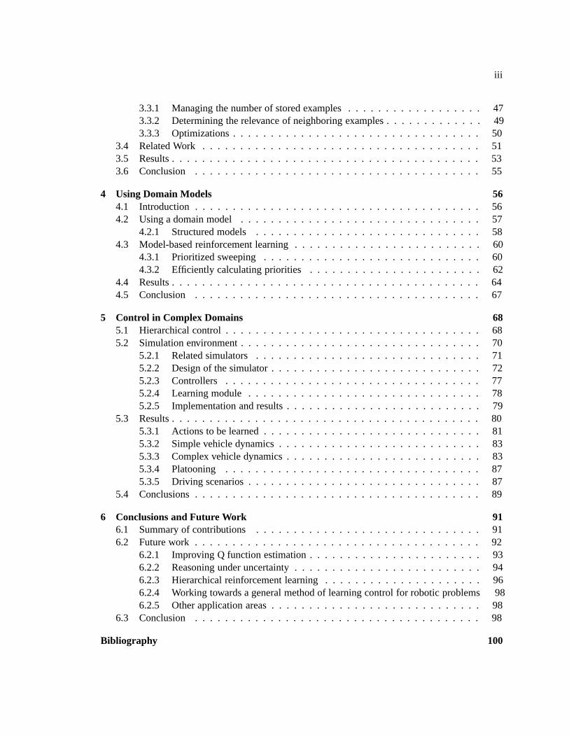
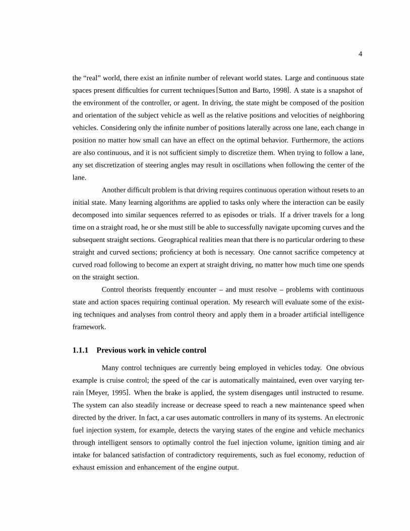
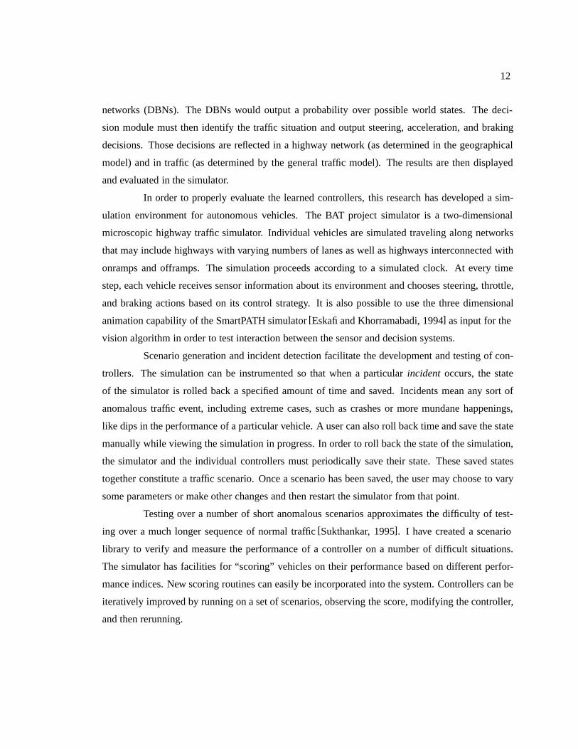
Figure 1.1: A view from the camera of the stereo vision system of Malik, et al, 1995. The rectanglesimposed on the vehicles in the image correspond to objects that the system detects. The right sideof the figure gives a virtual overhead view given the information from the vision system.

The main disadvantage of AVCS is that the technology is not mature enough to allow

for reliable driving except in controlled conditions [Bishop, 1997; Tokuyama, 1997]. The driving

environment is not readily handled by automatic control systems such as those already present in

3

the vehicle to control the various engine systems. The driving domain is complex, characterized by

uncertainty, and cannot be fully modeled by automatic control techniques.

These factors present an interesting challenge for artificial intelligence and control theory

necessitating the use of methods from various lines of inquiry:

� Temporal reasoning is needed to deal with time dependent events, sequences, and relation-

ships.

� Truth maintenance is useful because deduced facts may change over time.

� Real-time perception and action for effective and quick handling of unexpected asynchronous

events is required, since for an arbitrary event at an arbitrary state in the system, a response

must be available.

� Reasoning with uncertain or missing data is required. The environment is a difficult one with

unpredictable handling qualities, uncooperative or worse, antagonistic vehicles, and quirky

pedestrians.

� Adaptive behavior is essential, since it is not possible to consider all environments, vehicles,

and driving situations in the original design of a controller.

The driving problem thus can provide a rich testbed for “intelligent” algorithms.

The driving task itself is nicely decomposable. A driver tends to spend almost all of his or

her time in specific subtasks such as lane following, car following, or lane changing. The problem

of controlling a vehicle can generally be split into two parts: a lateral component that controls the

steering angle, and a longitudinal control component that controls the speed of the vehicle through

the throttle and sometimes the brake. In critical situations where extreme maneuvers are necessary,

the lateral and longitudinal control dynamics may not be independent. For example, turning the

wheel sharply while accelerating at full throttle is not advisable. Nevertheless, the actual steering

and throttle control decisions are almost always independent given a higher level command. For

example, given an acceleration trajectory and a lane change path, the longitudinal and lateral control

can be implemented independently. At higher levels, lateral and longitudinal control are also related.

If a lane change is the lateral action, the longitudinal action must take into account where the target

position is in the next lane and where the new lead vehicle will be.

Despite its decomposability, there a few aspects of driving that make it a particularly

difficult problem for artificial intelligence application. First, because of the continuous nature of

4

the “real” world, there exist an infinite number of relevant world states. Large and continuous state

spaces present difficulties for current techniques [Sutton and Barto, 1998]. A state is a snapshot of

the environment of the controller, or agent. In driving, the state might be composed of the position

and orientation of the subject vehicle as well as the relative positions and velocities of neighboring

vehicles. Considering only the infinite number of positions laterally across one lane, each change in

position no matter how small can have an effect on the optimal behavior. Furthermore, the actions

are also continuous, and it is not sufficient simply to discretize them. When trying to follow a lane,

any set discretization of steering angles may result in oscillations when following the center of the

lane.

Another difficult problem is that driving requires continuous operation without resets to an

initial state. Many learning algorithms are applied to tasks only where the interaction can be easily

decomposed into similar sequences referred to as episodes or trials. If a driver travels for a long

time on a straight road, he or she must still be able to successfully navigate upcoming curves and the

subsequent straight sections. Geographical realities mean that there is no particular ordering to these

straight and curved sections; proficiency at both is necessary. One cannot sacrifice competency at

curved road following to become an expert at straight driving, no matter how much time one spends

on the straight section.

Control theorists frequently encounter – and must resolve – problems with continuous

state and action spaces requiring continual operation. My research will evaluate some of the exist-

ing techniques and analyses from control theory and apply them in a broader artificial intelligence

framework.

1.1.1 Previous work in vehicle control

Many control techniques are currently being employed in vehicles today. One obvious

example is cruise control; the speed of the car is automatically maintained, even over varying ter-

rain [Meyer, 1995]. When the brake is applied, the system disengages until instructed to resume.

The system can also steadily increase or decrease speed to reach a new maintenance speed when

directed by the driver. In fact, a car uses automatic controllers in many of its systems. An electronic

fuel injection system, for example, detects the varying states of the engine and vehicle mechanics

through intelligent sensors to optimally control the fuel injection volume, ignition timing and air

intake for balanced satisfaction of contradictory requirements, such as fuel economy, reduction of

exhaust emission and enhancement of the engine output.

5

Recently, there have been a number of technologies to develop to give vehicles more au-

tonomy using control-theoretic techniques. In Autonomous Intelligent Cruise Control (AICC), the

car remains a speed-dependent target distance behind the preceding car at all times. AICC designs

use either radar, laser radar, infrared, or sonar sensing systems to determine the relative distance and

speed of the car in front [NAHSC, 1995]. Mitsubishi has an option on its Diamante model marketed

in Japan with an AICC system. Using a small Charge-Couple Device (CCD) camera and a laser

rangefinder, the vehicle maintains a preset following distance to the preceding car by adjusting the

throttle and downshifting if necessary. . A drawback to this feature is that the car has no data about

its environment other than the distance to the preceding object.

At UC Berkeley, the California Partners for Advanced Transit and Highways (PATH)

developed a system called platooning [Varaiya, 1991], in which vehicles travel at highway speeds

with small inter-vehicle spacing. This control is effected by adding extra equipment and logic to

both the vehicle and the roadside. Congestion can be reduced by closely packing the vehicles on

the highway and still achieving high throughput without compromising safety. The work done in

platooning is significant in that it demonstrates improved efficiencies with relatively little change to

the vehicles. However, platoons still run into some of the same problems as AICC where cars are

designed to operate only in a particular situation. Platoons cannot easily coexist with human driven

vehicles. This element limits the applicability of platoons to general driving conditions.

Lygeros et al. structure the platooning problem as a hierarchical hybrid control problem

so that strict guarantees can be made with regard to safety, comfort, and efficiency, given certain

operating conditions [Lygeros et al., 1997]. A hybrid system is one with interaction between con-

tinuous and discrete dynamics. In the hierarchy, the lower levels deal with local aspects of system

performance, such as maintaining a particular setpoint for a specific condition and for a particular

control law. The higher levels deal with the more global issues, like scheduling communication for

sharing resources between agents. The system itself is modeled as a hybrid automaton. The automa-

ton is a dynamical system describing the evolution of a number of discrete and continuous variables.

Given a hybrid automaton describing a system, a game theoretic scheme generates continuous con-

trollers and consistent discrete abstractions for the system. Using these formalisms, engineers can

design a safe, comfortable, and efficient system for longitudinal control of vehicles in platoons on

a automated highway system. Safety can be guaranteed by proving that from certain initial con-

ditions, no transitions can be made into the set of unsafe states in the hybrid automaton. Comfort

and efficiency are secondary concerns which are achieved by further guaranteeing that certain states

cannot be entered (e.g. the change in acceleration, jerk, never exceeds a certain magnitude).

6

There has been significant progress in road following with a variety of algorithms. The

vision system is used for lane marking and obstacle detection. Lane detection – through accurate

models of lane shape and width – can be developed a priori to yield robust estimates of the vehicle’s

position and orientation with respect to lane[Taylor et al., 1999]. Obstacle detection algorithms aim

to determine where other vehicles are in the field of view and report their size, relative position and

velocity by performing object recognition on individual images [Lutzeler and Dickmanns, 1998].

The information correlated between images in video is useful in determining motion [Kruger et

al., 1995] and in three dimensional object detection through binocular stereopsis as has been used

successfully to detect other vehicles on the highway in PATH’s StereoDrive project [Malik et al.,

1997] or to recognize city traffic, signs, and various obstacles in Daimler-Benz’s Urban Traffic

Assistant [Franke et al., 1998].

Systems utilizing computer vision techniques have shown promise in real-world proto-

types [Bertozzi et al., 2000]. The VaMP autonomous vehicle prototype developed at the Universitat

der Mundeswehr Munchen was driven autonomously for 95% of a 1600km trip from Munich, Ger-

many to Odense, Denmark. The human driver was in charge of starting lane change maneuvers,

setting the target speed, taking into account the destination and goals, and, of course, making sure

the automatic controller did not err and send the vehicle careening off the road or into another ve-

hicle. The ARGO prototype developed at the Dipartimento di Ingegneria dell’Informazione of the

Universita di Parma similarly drove itself for 94% of a 2000km safari through Italy [Broggi and

Berte, 1995; Broggi et al., 1999]. All of these approaches focus on the difficulties inherent in sens-

ing in the driving environment. The task of driving is performed using control-theoretic techniques.

The system takes the filtered sensor information and tracks a predetermined trajectory down the

center of the lane or from one lane to another.

The ALVINN project focused on developing driving algorithms through supervised learn-

ing [Pomerleau, 1993]. In supervised learning, the learner is given a set of training examples with

the corresponding correct responses. The goal of the learner is to use those examples to accurately

generalize and predict unseen examples: ALVINN “watches” an actual driver follow a lane for

about three minutes and then can perform the same basic maneuvers. The training examples con-

sist of a set of images and the corresponding steering wheel position. It uses a single hidden-layer

back-propagation neural network as a supervised learning algorithm[Bishop, 1995]. The system is

very proficient at performing maneuvers on different surfaces and in varying situations. However,

it is generally unable to deal with other uncooperative cars and is unable to perform tasks such as

lane changes or highway entry and exit.

7

Vision sensing can be quite robust, but difficulties arise in adverse lighting conditions,

such as glare. The work on these autonomous vehicles show that technology for lower-level control

is becoming increasingly viable. What remains to be achieved is the ability to recognize a particular

situation and then perform the appropriate maneuver.

Learning from proficient human drivers is a reasonable and intuitive method for develop-

ing autonomous vehicles. The challenge is to create controllers that work in almost all situations.

While driving proficiency can be achieved for basic situations, difficulties arise when trying to learn

the correct action in uncommon or dangerous scenarios. For example, the configuration where a car

is turned perpendicular to the direction of traffic (due perhaps to a spin on a slippery road) might

not appear while observing a human driver. An autonomous vehicle must perform competently in

this situation, and in whatever other scenarios it may encounter.

In order to deal with these kind of conditions, Pomerleau et. al would construct virtual

driving situations by rotating the image and recording a steering angle for this virtual image. These

virtual driving scenarios were Additionally, the engineers had to carefully control the learning en-

vironment. While it might seem that mimicking a human driver would provide a wealth of training

examples, it was actually a painstaking job for the researchers to select and formulate the correct

driving conditions. Presenting too many examples of one type would cause the system to lose pro-

ficiency in some other area. Filtering and reusing training examples along with constructing virtual

driving situations enabled ALVINN to learn to follow a lane.

Control by mimicking a human driver is problematic for a number of reasons. Any system

seeking to learn from human examples would have to overcome an impoverished situation repre-

sentation. A human driver has certain goals and concerns while driving that cannot be observed by

the system. Even if a system were able to compile years of examples from human drivers and be

able to reproduce it perfectly, the generalization will be poor and not well founded. There would be

no concept of trying to maximize performance; the task is only to copy previously seen examples.

Additionally, human decisions are at best optimal only for the particular human performing them. If

one human was replaced by another human at a subsequent time, the results may be far from ideal.

My attempt to use supervised learning for learning control of basic driving tasks exhibited all of

these problems and was not successful.

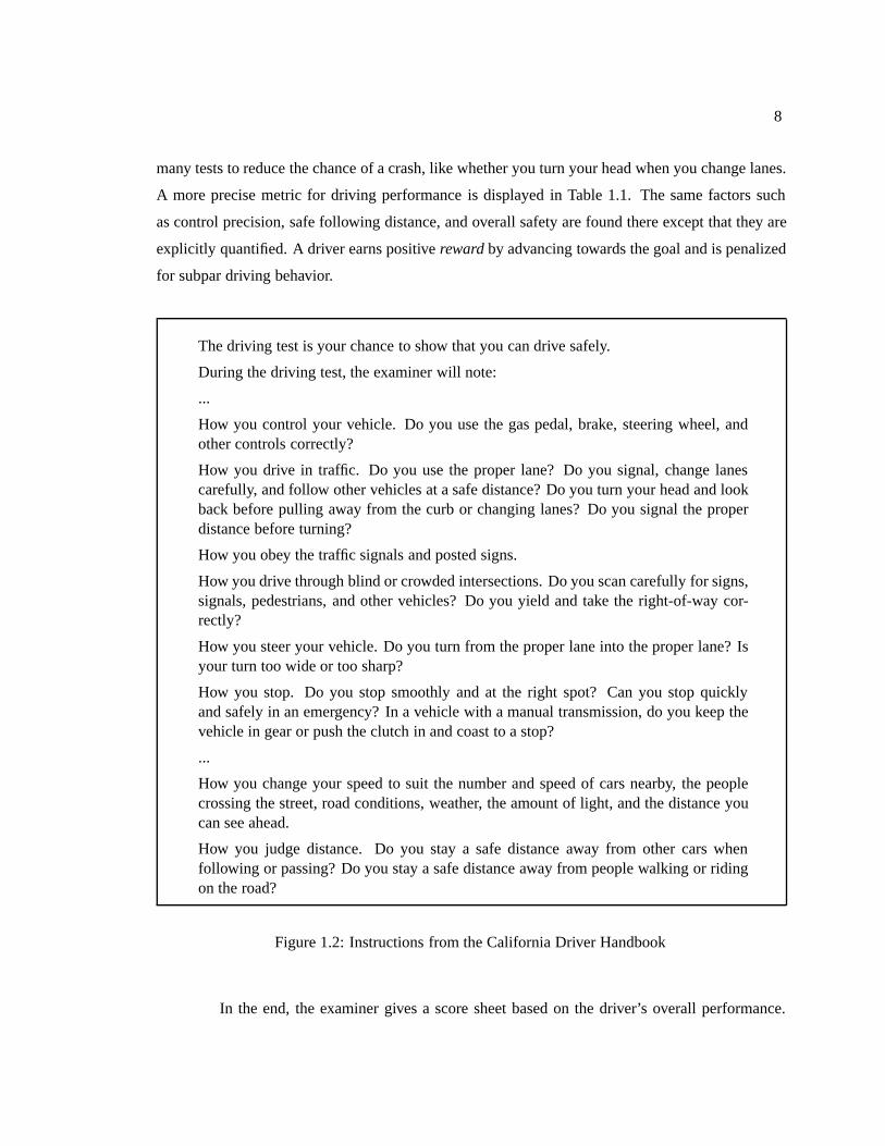
It is useful to study how human drivers are trained and evaluated. Below is the section

on the driver’s test, excerpted from the California Driver Handbook in Figure 1.2. The driving

evaluation criteria include measures of control precision, such as “How do you steer your vehicle?”

and “Do you stop smoothly?” Other factors included maintaining a safe following distance and

8

many tests to reduce the chance of a crash, like whether you turn your head when you change lanes.

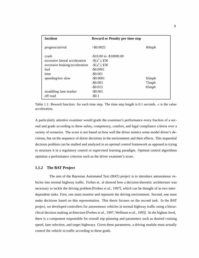
A more precise metric for driving performance is displayed in Table 1.1. The same factors such

as control precision, safe following distance, and overall safety are found there except that they are

explicitly quantified. A driver earns positive reward by advancing towards the goal and is penalized

for subpar driving behavior.

The driving test is your chance to show that you can drive safely.

During the driving test, the examiner will note:

...

How you control your vehicle. Do you use the gas pedal, brake, steering wheel, andother controls correctly?

How you drive in traffic. Do you use the proper lane? Do you signal, change lanescarefully, and follow other vehicles at a safe distance? Do you turn your head and lookback before pulling away from the curb or changing lanes? Do you signal the properdistance before turning?

How you obey the traffic signals and posted signs.

How you drive through blind or crowded intersections. Do you scan carefully for signs,signals, pedestrians, and other vehicles? Do you yield and take the right-of-way cor-rectly?

How you steer your vehicle. Do you turn from the proper lane into the proper lane? Isyour turn too wide or too sharp?

How you stop. Do you stop smoothly and at the right spot? Can you stop quicklyand safely in an emergency? In a vehicle with a manual transmission, do you keep thevehicle in gear or push the clutch in and coast to a stop?

...

How you change your speed to suit the number and speed of cars nearby, the peoplecrossing the street, road conditions, weather, the amount of light, and the distance youcan see ahead.

How you judge distance. Do you stay a safe distance away from other cars whenfollowing or passing? Do you stay a safe distance away from people walking or ridingon the road?

Figure 1.2: Instructions from the California Driver Handbook

In the end, the examiner gives a score sheet based on the driver’s overall performance.

9

Incident Reward or Penalty per time step

progress/arrival +$0.0025 60mph

crash -$10.00 to -$10000.00excessive lateral acceleration -$��excessive braking/acceleration -$��fuel -$0.0001time -$0.001speeding/too slow -$0.0001 65mph

-$0.003 75mph-$0.012 85mph

straddling lane marker -$0.001off road -$0.1

Table 1.1: Reward function: for each time step. The time step length is 0.1 seconds. � is the valueacceleration.

A particularly attentive examiner would grade the examinee’s performance every fraction of a sec-

ond and grade according to these safety, competency, comfort, and legal compliance criteria over a

variety of scenarios. The score is not based on how well the driver mimics some model driver’s de-

cisions, but on the sequence of driver decisions in the environment and their effects. This sequential

decision problem can be studied and analyzed in an optimal control framework as opposed to trying

to structure it in a regulatory control or supervised learning paradigm. Optimal control algorithms

optimize a performance criterion such as the driver examiner’s score.

1.1.2 The BAT Project

The aim of the Bayesian Automated Taxi (BAT) project is to introduce autonomous ve-

hicles into normal highway traffic. Forbes et. al showed how a decision-theoretic architecture was

necessary to tackle the driving problem [Forbes et al., 1997], which can be thought of as two inter-

dependent tasks. First, one must monitor and represent the driving environment. Second, one must

make decisions based on this representation. This thesis focuses on the second task. In the BAT

project, we developed controllers for autonomous vehicles in normal highway traffic using a hierar-

chical decision making architecture [Forbes et al., 1997; Wellman et al., 1995]. At the highest level,

there is a component responsible for overall trip planning and parameters such as desired cruising

speed, lane selection, and target highways. Given these parameters, a driving module must actually

control the vehicle in traffic according to these goals.

10

The driving module itself can be split up further where it may call upon actions such as

lane following or lane changing. Some interaction between levels will exist. For example, an action

such as a lane change must be monitored and in some cases aborted. The problem is decomposed

wherever possible, keeping in mind that there will always be potential interactions between different

tasks. One can first consider the actions as immutable, atomic actions with a length of 1 time step.

A set of actions can be classified as follows:

� Lateral actions

– Follow current lane

– Initiate lane change (left or right)

– Continue lane change

– Abort lane change

– Continue aborting lane change

� Longitudinal actions

– Maintain speed (target speed given from environment)

– Maintain current speed

– Track front vehicle (following distance given by environment)

– Maintain current distance

– Accelerate or decelerate (by fixed increment such as 0.5 ��)

– Panic brake

The BAT architecture is described in Figure 1.3. The decision module is passed percep-

tual information (percepts). The goal is to eventually use a vehicle that is fitted with a number of

cameras that provide input to the stereo vision system which would determine the positions and

velocities of other vehicles, along with data on the position of the lane markers and the curvature of

the road [Luong et al., 1995]. Sample output from the stereo vision system is shown in Figure 1.1.

This research focuses on the control and decision making aspects rather than the interaction be-

tween the control and sensing. One cannot reasonably and safely develop control algorithms with a

real vehicle, so instead all control is performed in a simulation environment with simulated sensor

readings. The decision module then take the percepts and monitor the state using dynamic Bayesian

11

Sensors

Danger?

Yes No

EvasiveManeuver

Too Fast?

Yes No

Slow Down Cruise

Decision Trees

Probability

Velocity

Probability Distribution

Belief Networks

ActionFigure 1.3: How the BAT itself is expected to work. Given data from the sensors, the agent deter-mines the probability distribution over world states using belief networks. From there, the agentusing a hierarchical decision making structure to output a control decision.

12

networks (DBNs). The DBNs would output a probability over possible world states. The deci-

sion module must then identify the traffic situation and output steering, acceleration, and braking

decisions. Those decisions are reflected in a highway network (as determined in the geographical

model) and in traffic (as determined by the general traffic model). The results are then displayed

and evaluated in the simulator.

In order to properly evaluate the learned controllers, this research has developed a sim-

ulation environment for autonomous vehicles. The BAT project simulator is a two-dimensional

microscopic highway traffic simulator. Individual vehicles are simulated traveling along networks

that may include highways with varying numbers of lanes as well as highways interconnected with

onramps and offramps. The simulation proceeds according to a simulated clock. At every time

step, each vehicle receives sensor information about its environment and chooses steering, throttle,

and braking actions based on its control strategy. It is also possible to use the three dimensional

animation capability of the SmartPATH simulator [Eskafi and Khorramabadi, 1994] as input for the

vision algorithm in order to test interaction between the sensor and decision systems.

Scenario generation and incident detection facilitate the development and testing of con-

trollers. The simulation can be instrumented so that when a particular incident occurs, the state

of the simulator is rolled back a specified amount of time and saved. Incidents mean any sort of

anomalous traffic event, including extreme cases, such as crashes or more mundane happenings,

like dips in the performance of a particular vehicle. A user can also roll back time and save the state

manually while viewing the simulation in progress. In order to roll back the state of the simulation,

the simulator and the individual controllers must periodically save their state. These saved states

together constitute a traffic scenario. Once a scenario has been saved, the user may choose to vary

some parameters or make other changes and then restart the simulator from that point.

Testing over a number of short anomalous scenarios approximates the difficulty of test-

ing over a much longer sequence of normal traffic [Sukthankar, 1995]. I have created a scenario

library to verify and measure the performance of a controller on a number of difficult situations.

The simulator has facilities for “scoring” vehicles on their performance based on different perfor-

mance indices. New scoring routines can easily be incorporated into the system. Controllers can be

iteratively improved by running on a set of scenarios, observing the score, modifying the controller,

and then rerunning.

13

1.1.3 Driving as an optimal control problem

Controlling an autonomous vehicle is best formulated as a stochastic optimal control prob-

lem. Driving presents the problem of delayed reinforcement. Rarely does the action which immedi-

ately precedes an event, such as a crash, deserve the blame or credit. For example, the action which

usually precedes a crash is maximum braking, but the action of maximum braking rarely causes

the crash. Instead, the degree of success or failure must be judged by some performance index or

reward function: in following the center of a lane, a reward function would take into account the

deviation from the center of the lane and might consider the smoothness of the ride, determined

by the magnitude of the lateral acceleration. A controller that was able to perform optimally with

respect to these criteria would be ideal.

Driving can easily be modeled as a sequential decision problem, with time divided into

discrete units. The autonomous driving agent makes a sequence of control decisions at every time

step (e.g. steer left 2 degrees and hold throttle at 10 degrees) and receives reward or penalty. In the

end, our goal is to calculate the optimal policy for various driving tasks. The control decisions have

delayed effects that must be considered in choosing the action to take in each state. A policy that

chooses actions solely for their immediate effects may not be optimal over the long term. However,

calculating the optimal policy for nontrivial environments is generally intractable. As will be shown

in the discussion of reinforcement learning in Section 2.1, we can still develop quite proficient

policies by adjusting the policy from the results of the agent’s experiences in the environment.

There has been a great deal of work in optimal control and Markov Decision Processes

(MDPs) in formalizing these sequential decision problems. In MDPs, the optimal mapping from

world configurations (states) to optimal behavior (policy) is determined entirely by the expected

long-term return from each state, called its value. Reinforcement Learning (RL) algorithms can

learn optimal behavior in MDPs from trial and error interactions with the environment. However,

reinforcement learning algorithms often are unable to effectively learn policies for domains with

certain properties: continuous state and action spaces, a need for real-time online operation, and

continuous operation without degrading performance.

1.2 Summary of contributions

The question this dissertation addresses is how to learn to control a car for the longitudinal

and lateral actions described earlier in the domains characterized in Section 2.3. My thesis is that

14

reinforcement learning utilizing stored instances of past observations as value estimates is an effec-

tive and practical means of controlling dynamical systems such as autonomous vehicles. I present

the results of the learning algorithm evaluated on canonical control domains as well as automobile

control tasks.

I present a new method for estimating the value of taking actions in states by storing

relevant instances that the agent experiences. As the agent learns more about the environment,

the stored instances are updated as well so that our value function approximation becomes more

accurate. This method uses available resources to remain robust to changing tasks and is shown to

be effective in learning and maintaining a value estimate for problems even as the task changes.

I also develop a general intelligent control architecture for the control of autonomous ve-

hicles. From the testing environment to the decomposition of the driving task, this research extends

and combines a number of techniques in developing proficient vehicle controllers. I propose a hi-

erarchical model-based solution integrating a number of new methods from reinforcement learning

to address vehicle control. The algorithm is effective on canonical control domains as well as more

complex driving tasks. Section 2.3 details the characteristics of the domains of interest. Section 2.4

describes the research problem more fully.

1.3 Outline of dissertation

The structure of this dissertation is as follows. I describe the field and related work in

reinforcement learning and control and explicitly state the thesis problem in Chapter 2. Given that

background, Chapter 3 introduces an effective method for instance-based value function approxima-

tion. The chapter describes the instance-based reinforcement learning algorithm and its extensions

to standard reinforcement learning applications as well as some results on some canonical domains.

Chapter 4 shows how I use a structured domain model to learn more efficiently and handle funda-

mental autonomous vehicle tasks. Chapter 5 explains how we can apply those control vehicle tasks

in creating a more general autonomous vehicle controller and describes my simulation environment.

Finally, Chapter 6 presents conclusions and suggests some future directions for research. scp

15

Chapter 2

Reinforcement Learning and Control

Developing effective reinforcement learning techniques for control has been the goal of

this research. This chapter discusses various approaches to control. I introduce the cart-centering

domain and use it to demonstrate classical control, optimal control, and reinforcement learning

algorithms. Reinforcement learning (RL) has been shown to be an effective technique for deriving

controllers for a variety of systems. This chapter gives some of the necessary background for the

ensuing discussion of RL.

Driving is a particularly challenging problem, since the task itself changes over time;

i.e. there is a nonstationary task distribution. As explained in Chapter 1, a lane following agent

may become proficient at negotiating curved roads and then go on a long straight stretch where it

becomes even more proficient on straight roads. It cannot, however, lose proficiency at the curved

roads. The overall goal of staying in the center of the lane remains the same, but the kind of states

that the agent is faced with changes when moving from curved roads to straight and back again.

Many learning algorithms are vulnerable to catastrophic interference where, after expe-

riencing numerous new examples in a different part of the state space, accuracy on older examples

can decrease. This behavior is referred to as forgetting. Section 2.2 explains this problem more

formally. As in real life, forgetting is obviously inadvisable in any learning control algorithm.

This chapter examines the problem of reinforcement learning for control with particular

focus on how forgetting is a problem for most adaptive methods. Section 2.3 describes the control

environments of interest and their characteristics. Finally, the research problem that this dissertation

addresses is explicitly stated in Section 2.4.

16

2.1 Background

Reinforcement learning is generally defined as adapting and improving behavior of an

agent through trial and error interactions with some environment [Kaelbling et al., 1996]. This

broad definition can include a vast range of algorithms from a word processing program that sug-

gests completions to currently incomplete words to a program which at first behaves randomly but

eventually produces a new economic system for eliminating world hunger. This definition imposes

few constraints on how exactly the improvement is achieved. One key commonality of all rein-

forcement learning algorithms is that they must have some sort of performance metric by which the

agent is judged. Performance metrics for the previous problems might be keystrokes pressed by the

user or the number of hungry children. In this section, I will define my particular methodology and

scope.

The first step is to instroduce some of the basic terminology to be used in discussing

reinforcement learning. A state is an instantaneous representation of the environment. The repre-

sentation of the environment that the agent perceives are called the percepts. The discussion in this

dissertation assumes that the percepts are equivalent to the state meaning that the environment is

fully observable. I denote the state at time � as a real valued vector with �� elements, �� ,

��, or more simply as �. An action is the position of the agent’s actuators at some time �, which is

represented as �� . In a sequential decision problem, the agent moves through the

state space taking actions at each state. For example, a possible trajectory would be defined as a

sequence of state-action pairs:

��

where �� is the initial state, �� is the final terminal state, and � is the null or no-op action. Where

the task is not episodic and there is not a terminal state, there can exist an unbounded sequence of

state-state action pairs �� where � � � �. An input � is defined as one of these state-action

pairs: �� and the input at time �, ��, is ��.

The behavior of an agent is determined by its policy. A policy is a mapping from

states to actions that specifies what the agent will do in every situation so that �� . A

reward function �� is a scalar function given by the environment that gives some performance

feedback for a particular state and action. I will refer to the reward at time �, ��, as ��. It is

often useful and appropriate to discount future rewards using a discount rate, � �� . Reaching

the goal now is much better than doing nothing then reaching the goal in 10 years, and, similarly, a

17

car crash now is much worse than one in a decade. More precisely, a reward received k steps in the

future is worth � times a reward received now. The goal of the agent is to construct a policy that

maximizes the total accumulated discounted reward,��

�� . For finite horizon problems where

the total number of steps in an episode is � , the goal is to maximize��

�� , where ��

is the final terminal reward. A control problem consists of:

1. A mathematical model of the system to be controlled (plant) that describes how the state

evolves given a previous state and an action;

2. Bounds on the state and action variables;

3. Specification of a performance criterion (e.g. the reward function).

A control policy’s effectiveness is determined by the expected total reward for an episode.

The reward function alone does not provide enough information to guarantee future rewards from

the current state. Determining which in a series of decisions is responsible for a particular delayed

reward or penalty is called the temporal credit assignment problem. Temporal difference methods

attempt to solve the temporal credit assignment problem by learning how an agent can achieve

long-term reward from various states of its environment [Gordon, 1995].

Methods that learn policies for Markov Decision Processes (MDPs) learn the value of

states. The value of a particular state indicates the long term expected reward from that state:

� ��

�� (2.1)

This mapping from states to value is referred to as the value function. The state representation in

a MDP must obey the Markov property where future is independent of the past given the present.

More precisely, given a traditional MDP with discrete states � � � and actions � � �, where

�� is the probability of moving from state �� to state �� using action ��, the Markov

property guarantees that

��

Practically, this property means that the state representation must encapsulate all that is relevant

for further state evolution. A common solution to any problem currently not Markovian is to add

all possible information to the state. In driving, for example, it is sufficient to see a snapshot of a

neighboring car in between lanes; one must also know whether that vehicle is in midst of a lane

18

change or just straying outside its lane. This information about lateral intentions can be added to

the state and thus augment the information given in the snapshot.

Given an accurate representation of the value function defined in Equation 2.1, an agent

can act greedily, moving to the state that has the highest value. The policy is then

��

��

��

��

�� (2.2)

This policy � is the optimal mapping from states to actions, i.e. the one that leads to the highest

sum of expected rewards. The continuous state and action analog is:

��

��

�� (2.3)

where �� is the transition probability density function that describes the probability of mov-

ing from state � to state �� by applying action �.

Instead of calculating a value function to choose actions, some algorithms learn a policy

directly. These methods search the space of policies to maximize reward, taking a set of policies,

�, and improving them through repeated evaluations in the domain. The set of policies may be

randomly initialized or use some previously computed suboptimal example. The number of policies

may be one or some greater number to do multiple searches in different areas of the policy space.

The policies are improved iteratively according to the general scheme in Figure 2.1. Examples of

procedure PolicySearch ()loop

(1) Remove a policy from �(2) evaluation accumulated reward for episode starting from initial state ��(3) Adjust policy based on evaluation(4) Insert into �

Figure 2.1: Policy search algorithm

Basic framework for algorithms that search within the space of policies

these types of policy search algorithms are genetic programming, evolutionary algorithms, and hill

climbing algorithms. These methods have been shown to be effective in learning policies for a

number of domains [Whitley et al., 2000]. Nevertheless, learning a value function has a number of

advantages over direct policy search. Since learning is over states rather than episodes, the learning

process itself is more finely grained. Learning on a state by state basis can differentiate more quickly

19

between subtly differing policies. This refinement can be especially useful in domains where the

set of reasonable policies is much smaller than the overall policy space, often the case in control

domains. For example, while there are a large variety of steering positions and throttle angles,

driving uses a limited subset of them. Going straight and neither accelerating nor braking tends to

be a reasonable policy most of the time. The difficulty is in differentiating the less common cases

where turning or speed modulation is necessary. Another advantage of learning a value is that if

the episodes themselves are very long or even without end, any method which learns on an episodic

basis may not have enough opportunity to improve policies. In terms of diagnosing the behavior of

the system, a final benefit is that the value function offers a snapshot of an agent’s “beliefs” at any

time.

There are disadvantages to using the indirect method of calculating a value function in-

stead of calculating a policy directly. Sometimes a policy can be more easily represented than a

value function and computing the value function may be difficult and unnecessary to the overall

goal of learning a policy. Policy search has been shown to compute reasonable solutions for many

problems efficiently. There is currently research looking into ways of doing direct policy search in

sequential decision problems, where learning a value function is no longer necessary but learning

is done on a state by state basis rather than per episode [Ng and Jordan, 2000]. For the remainder

of this dissertation, I will restrict my discussion of reinforcement learning to those methods that

learn optimal control in MDPs. Moreover, I assume that the state transition model is unknown and

learning is accomplished by adjusting an estimate of value of states.

2.1.1 Optimal control

Optimal control has its roots in classic regulatory control but tries to broaden the scope.

The goal in regulatory control is to force plant states to follow some trajectory. The state trajectory

is the history of states, �� in the time interval �� . The target states are referred to as

setpoints. The objective of optimal control instead is “to determine the control signals that will

cause a process to satisfy the physical constraints and at the same time minimize (or maximize)

some performance criterion.”[Kirk, 1970] The optimal control perspective is similar to that of

Markov Decision Processes. The divergences tend to stem from the difference in practitioners and

applications. Optimal control is generally the realm of control theorists, while Markov decision

processes are the framework of choice in artificial intelligence and operations research communi-

ties. In optimal control, most systems are described by a set of differential equations which describe

20

the evolution of the state variables over continuous time in a deterministic environment as opposed

to the discrete time, stochastic environments of MDPs. Additionally, optimal control deals with

problem in continuou Optimal control and related optimization problems have their roots in antiq-

uity [Menger, 1956]. Queen Dido of Carthage was promised all of the land that could be enclosed

by a bull’s hide. Not to be cheated out of a fraction of a square cubit of her property, she cut the hide

into thin strips to be tied together. From there, her problem was to find a closed curve that encloses

the maximum area. The answer was, of course, a circle. In coming up with a general answer to this

question, the Queen had stumbled upon the roots of the Calculus of Variations. Variational calculus

is essential in finding a function, such as a policy, that maximizes some performance measure, such

as a reward function.

Markov decision processes are a relatively new formulation that came out of optimal con-

trol research in the middle of the twentieth century. Bellman developed dynamic programming,

providing a mathematical formulation and solution to the tradeoff between immediate and future

rewards [Bellman, 1957; Bellman, 1961]. Blackwell [Blackwell, 1965] developed temporal differ-

ence methods for solving Markov Decision Processes through repeated applications of the Bellman

equation

� ��

�� (2.4)

where the expected value is respect to all possible next states �� and given that the current state is �

and the action chosen is �.

The two basic dynamic programming techniques for solving MDPs are policy iteration

and value iteration. In policy iteration [Howard, 1960], a policy is evaluated to calculate the value

function � �. For all � in our state space �,

� ��

�� (2.5)

�� is the transition probability from state � to state �� given that the action determined by

our policy �� is executed. The set of these transition probabilities for an environment is referred

to as the model. Evaluating a policy requires either iteratively calculating the values for all the states

until � � converges or solving a system of linear equations in �� steps [Littman et al., 1995].

Then, is improved using � � to some new policy �. For all �,

��

��

��

��

�� (2.6)

The policy evaluation and policy improvement steps are repeated until the policy converges (i.e.

� � ��) which will happen in a polynomial number (in the number of states and actions) of

21

iterations if the discount rate, , is fixed. Value iteration [Bellman, 1957] truncates the policy

evaluation step and combines it with the policy improvement step in one simple update:

��

��

�� (2.7)

The algorithm works by computing an optimal value function assuming a one step finite horizon

and then assuming a two-stage finite horizon and so on. The running time for each iteration of value

iteration is ��. For fixed discount rate, , value iteration converges in a polynomial number

of steps. While value iteration and policy iteration are useful for solving known finite MDPs, they

cannot be used for MDPs with infinite state or action spaces, such as continuous environments.

Reinforcement learning is concerned with learning optimal control in MDPs with un-

known transition models. Witten [Witten, 1977] first developed methods for solving MDPs by

experimentation. RL has become a very active field of research in artificial intelligence[Kaelbling

et al., 1996; Sutton and Barto, 1998].

2.1.2 The cart-centering problem

To best understand the different approaches, it is useful to see how they work in the context

of a specific problem domain. For example, consider a cart-centering problem [Santamaria et al.,

1998]. Imagine that there is a unit mass cart which is on a track. The cart has thrusters which allow

it to exert a force parallel to the track. The goal is to move the cart from an initial position to a

position in the center of the track at rest. The cart is able to measure its position with respect to the

goal position and its velocity.

Let the position of the cart be �; the velocity of the cart is the derivative of �: �� . The

state vector in this case will be � � �� and the goal state �� . The force applied to

the cart is � . Since the cart is of unit mass and � � �� by Newton’s second law, the acceleration

applied to the cart is equal to � . The dynamics of the cart can be defined as:

� � �� (2.8)

� � � � �� (2.9)

In vector notation, that is:

��

��

��

��

��

��

��

��

� �

��

��

��

��

�

�� (2.10)

� �� (2.11)

22

The change in the state �� can be expressed as

�� (2.12)

Control-theoretic approaches

One can see that this system has linear dynamics and bidimensional state. The system is

commonly referred to as the double integrator, since the velocity is the integral of the acceleration

action and the position is then the integral of the velocity. While the system is relatively simple, it

does exhibit many important aspects of the sequential decision problems I hope to address, including

delayed feedback, multiple performance criteria described below, and continuous state and action

spaces. One can compute the optimal policy for this environment using control-theoretic techniques.

The desired goal position � � �� is referred to as the setpoint.

Feedback control can be defined as any policy that depends on the actual percept history

of a controlled system. Corrections are made on the basis of the difference between the current

state and the desired state. A common strategy is to use feedback control where corrections are

made on the basis of this error. A controller employed in domains such as this one is the feedback

Proportional plus Derivative (PD) Compensator [Dubrawski, 1999]:

� � ��

where � is the error from the setpoint. In the case of the cart-centering problem, � � � and

�� . Given this formulation, all that is left is calculating the coefficients � and ��, also

called the gains. In order to analytically derive the gains, it is necessary to generate the transfer

function for the combination of the controller and the environment. Where it is not possible to

match the system exactly to some easily expressed linear model, the PD gains can be computed

using a root locus design approach. Most systems have nonlinear elements, but, assuming that

the system operates over a small portion of the state space, controllers designed for linear sys-

tems may still be successful. The methods for control of linear time-invariant systems are well

known. A control theory text gives ample details on these methods [Kumar and Varaiya, 1986;

Nise, 2000]. Truly nonlinear systems are more difficult to control because the system is not solv-

able. In this case, solvable means that the one can solve the differential equations that describe

the dynamics and derive closed-form equations that describe the behavior of the system in all

situations. Algorithms to solve nonlinear control problems include bifurcation and chaos analy-

sis [Sastry, 1999]. With these more advanced techniques, the system must be completely described

23

in precise terms in order to successfully apply nonlinear control. Even for domains in which the

optimal policy is relatively simple, determining it with these techniques may be extraordinarily dif-

ficult. Control theory focuses on systems where the behavior can be completely specified so that the

feedback the controller provides will produce an overall system that behaves as desired.

Some problems are more naturally described within an optimal control framework. One

may not know the desired setpoints but still some reward function to maximize or cost function to

minimize. To make the cart’s ride more smooth, one might want to penalize the use of large forces.

This smoothness criterion adds a penalty or cost to actions and turns the problem into an optimal

control problem. Let the instantaneous penalty be a negative quadratic function of the position and

the acceleration applied. The reward, the opposite of the penalty, is then

��

or in vector representation:

��

� �� (2.13)

where � is

��

� �

�� and � is

�. The accumulated reward or value is expressed in terms

of continuous time. Let � be the continuous time reward function over states, actions, and time

intervals, then the performance measure for an episode running from �� to �� is

� � ��

�� (2.14)

Systems of this form with linear dynamics and quadratic performance criteria are com-

mon and are referred to as linear-quadratic regulator problems[Astrom, 1965; Kirk, 1970]. Using

the Hamilton-Jacobi-Bellman equation yields a closed-form solution for the continuous regulator

problem. The Hamilton-Jacobi-Bellman equation is:

� � � � � �� (2.15)

The solution to Equation 2.15 is (from [Santamaria et al., 1998]):

� �� (2.16)

� ��

where P is

�� (2.17)

24

The optimal control policy for this problem is time invariant. In fact, all policies for the control

problems discussed hereafter are assumed to be time invariant. This presupposition follows from

the Markov property and will be discussed more in Section 2.3. For time invariant policies, ��

as � � �. The solution for P is then

��

� �

� �

��. From 2.16, the optimal value function is

� �� . The gain matrix is

� � ��

� �

(2.18)

which gives us the optimal control law:

�� (2.19)

For a “real-life” cart-centering problem, the track likely will not stretch arbitrarily in both

directions. If the track is bounded and a cart that moves too far from the goal position falls into

a pit of fire, then this formulation is not entirely accurate and the analysis is no longer complete.

The effect is to add a set of terminal states �� which is defined as all states from the original set �

where � �� or � � ��. The reward function must be changed so that �� .

The reward function is no longer simply quadratic and the guarantees of optimal behavior no longer

apply. In this case, the policy in Equation 2.19 still performs optimally for the region around the

goal state.

Even for those problems which can be described in this formulation, computing the solu-

tion to the Hamilton-Jacobi-Bellman equation is nontrivial. The calculus of variations has been used

to determine a function that maximizes a specified functional. The functional for optimal control

problems is the reward function. Variational techniques can be used in deriving the necessary con-

ditions for optimal control. Integrating the matrix differential equation of Equation 2.15 can yield

the optimal control law. However, the boundary condition leads to a nonlinear two-point boundary-

value problem that cannot be solved analytically to obtain the optimal control law. Instead, nu-

merical techniques are used. Three popular techniques are steepest descent, variation of extremals,

and quasi-linearization. These methods compute an open-loop optimal control which gives a se-

quence of control decisions given some initial state. Optimal control texts[Sastry and Bodson, 1989;

Kirk, 1970; Bellman, 1961] give a thorough treatment of these techniques.

Unfortunately for engineers, most control problems are not accurately described as linear

quadratic regulators. Non-linear systems, on the other hand, are much more difficult to control than

linear systems using these techniques. The core difficulty lies in deriving the solution to the set of

25

non-linear differential equations. Linear systems theory is well developed. In many cases, it can

be proven that a system is stable and converges. Stability means that small perturbations of the

system’s initial conditions or parameters do not result in large changes in the system behavior. A

system that is asymptotically stable tends toward the goal state in the absence of any perturbations.

Nevertheless, many systems of interest are non-linear. Systems in nature are exceedingly non-

linear, yet biological motor control systems are able to effectively control their biological actuators

(i.e. muscles) for various tasks. In nature, it is not necessarily important that one be able to prove the

bounds of behavior in all possible state configurations, but it is important not to die unnecessarily.

2.1.3 Learning optimal control

An important component of human intelligence and skill is the ability to improve perfor-

mance by practicing a task. In learning, policies are refined on the basis of performance errors[An

et al., 1988]. Learning can also reduce the need for an accurate model of the dynamics of a system

as the environment itself can be the model. As an internal model is made more accurate, both initial

performance and efficiency of learning steps are improved. Of course, learning algorithms can also

take advantage of knowledge about the environment. The use of models in learning algorithms is

revisited in Chapter 4.

The first step is to look at a model-free reinforcement learning algorithm called Q learning.

In Q learning, the agent learns a Q-function �� which gives the value of taking an action

� in a state �. The Q-function, �� and the value function � �� are closely related:

��

�� (2.20)

where is the discount factor and �� is the transition probability density function of going

from our current state � to some new state �� using action �. Conversely, � can be defined from �

as:

� �� (2.21)

Q learning is a “model-free” learning algorithm because it is not necessary to learn the transition

probabilities in order to learn the Q function. Considering the problem with discrete states and

actions first, the Q-function can be represented as a table with one entry for every state-action pair.

If the set of states is � and the set of actions is �, then the number of Q-function entries will be

��. Each of these entries can be set to some initial value. The Q estimates are updated in

response to experience. Given that the agent is in state �� at some time � and chooses action ��,

26

it then receives the associated reward ��, and arrives at state �� at time � � �. From ��, the

agent then chooses an action ��. This quintuple of events �� is referred to as

a SARSA (state action reward state action) step. The predicted value of taking the action �� in state

�� is �� . The value that the agent observes is the instantaneous reward it receives in �� (��)

plus the discounted value of the next state, �� . The Q estimate has converged when the

predicted and observed values are equal for all states. The Q-function update takes a step to make

the difference between the observed and predicted values smaller. The update equation is then:

�� (2.22)

where � � �� is the learning rate.

Q-learning is guaranteed to eventually converge to the optimal control strategy given a

number of assumptions. The learning rate at time step �, �, must have the following characteristics:

� � � � (2.23)� �� (2.24)

An example of such a function is �� . The environment must be finite, Markovian, and

stationary. If the agent visits all states and picks all actions an infinite number of times and the

policy converges in the limit to the greedy policy (Equation 2.2), the Q estimate will converge to

the optimal, true Q-function �� with probability 1. These results would not apply to my domains

of interest because they do not have finite state or action spaces. An MDP is stationary if the reward

function and state transition probabilities are independent of time.

Reinforcement learning has been applied with good results in a number of domains. The

first prominent reinforcement learning program was Samuel’s checkers playing program[Samuel,

1959]. Samuel used heuristic search methods and temporal difference methods to learn to play

checkers by playing games against itself and some human players. The checkers-playing program

achieved an above-average skill level and attracted much attention when it was demonstrated on

television in 1956. Tesauro developed a backgammon program that reached a grand-master level

of play using reinforcement learning techniques [Tesauro, 1992]. Other successful applications

of reinforcement learning have included dynamic channel allocation for cellular telephones and

scheduling algorithms [Zhang and Dietterich, 1996; Crites and Barto, 1996].

Reinforcement learning has also been used in the vehicle control domain. In general,

the problem has been restricted by using a relatively small number of discrete actions. Pyeatt and

Howe [Pyeatt and Howe, 1998] use RL to learn how to race around an oval track where the steering

27

angle can be incremented or decremented by a preset amount. Andrew McCallum’s thesis applies

a reinforcement learning algorithm to a problem where the positions in the lanes are discretized

[McCallum, 1995]. At each step, the car can either move one step forward or move into the adjoining

lane on the right or left. In order to realistically drive an actual vehicle, the driving environment and

actions must be treated as continuous.

2.1.4 Value function approximation

Given the continuous state and action space, some sort of function approximation is nec-

essary, since it would be impossible to represent the value function using a table. The normal

method is to use some sort of parametric method such as a neural network to approximate the value

function.

The neural network represents the approximate Q-function �� !� � " �� !�� where

� � �#�� #�� #�� is a vector of weights or parameters for " , the function represented by the

neural network. The Q-function estimate is updated by first calculating the temporal difference

error, � , the discrepancy between the value assigned to the current state and the value estimate for

the next state:

� �� (2.25)

The error for the SARSA update is accordingly:

� �� (2.26)

Equation 2.26 and Equation 2.25 are different with probability $, the exploration probability. These

updates are identical to a TD(0) policy evaluation step. The weights� that parameterize the function

approximator " �� are then updated according to the following rule:

� �� (2.27)

For a finite environment, the Q-function converges to

��

�� (2.28)

The conditions for convergence are that the environment must have be finite, Marko-

vian, and stationary. Clearly, the driving environment is not finite. Moreover, Q-learning will

not necessarily converge when using a nonlinear function approximator like a multi-layer neu-

ral network. While these methods are not guaranteed to converge, there is promise that the al-

gorithm using function approximation will remain near a good if suboptimal solution and there

28

are convergence guarantees for some linear and nonlinear cases [Tsitsiklis and Van Roy, 1997;

Papavassiliou and Russell, 1999; Gordon, 2001].

2.2 Forgetting in parametric function approximators

I have previously shown that driving does not necessarily have a stationary task distribu-

tion. Consider the task of trying to remain in the center of a lane. A driver may encounter long

stretches of straight roads with curved segments appearing infrequently and irregularly. In trying

to learn the value function from experience, a parametric function approximator such as a neural

network would develop a reasonable estimate. The car’s behavior would improve and it would be

able to drive near the center of the lane for a period of time. Eventually though, the system would

become unstable as the approximator would forget and its behavior would deteriorate. The unlearn-

ing would occur because the distribution of states tends to focus more and more in the center of the

lane. These new examples interfere with the approximator’s estimate of the value of less common

states such as positions farther away from the center of the lane. This catastrophic interference is a

common problem in the neural network control literature [Weaver et al., 1998].

The problem occurs because examples from the past have a vanishing effect on our current

approximation of the value function. These examples may be uncommon but are still crucial for

maintaining an accurate estimate for the entire relevant example space. Beyond losing accuracy for

these less recently seen regions of the example space, forgetting can also affect the shape of the

value function. As the approximator tries to fit the aforementioned middle of the road examples, the

estimate will become flatter. This effect is shown in Figure 2.2. The shape of value function is more

important than the actual values in terms of its effect on overall policy, since the action chosen at

every state is that with the maximum value, �� . The effect of the catastrophic

interference depends on the particular function approximation technique. Changing the shape of the

value function can affect the policy for distant states.

The effect of interference can be lessened by changing the experimental setup. Instead of

trying to learn directly from the learning agent’s experiences on the given task, the set of experiences

can be tailored to the learning algorithm. Learning can be done off policy where a set of experiences

�� are given as a set to the learning algorithm. The experiences can then be presented

repeatedly in different orders. Another alternative is to arrange the experiment so that the relevant

important examples are shown equally. The example distribution can be manually synthesized and

controlled to limit the effects of interference. For eample, learning might only occur over alternating

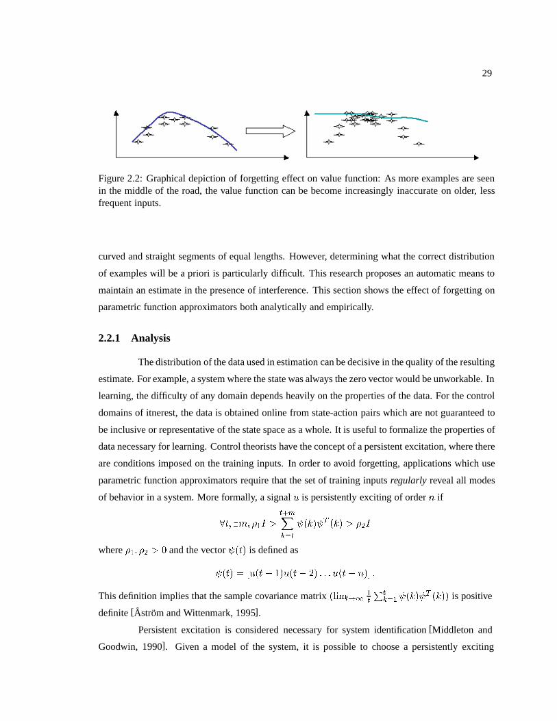
29

Figure 2.2: Graphical depiction of forgetting effect on value function: As more examples are seenin the middle of the road, the value function can be become increasingly inaccurate on older, lessfrequent inputs.

curved and straight segments of equal lengths. However, determining what the correct distribution

of examples will be a priori is particularly difficult. This research proposes an automatic means to

maintain an estimate in the presence of interference. This section shows the effect of forgetting on

parametric function approximators both analytically and empirically.

2.2.1 Analysis

The distribution of the data used in estimation can be decisive in the quality of the resulting

estimate. For example, a system where the state was always the zero vector would be unworkable. In

learning, the difficulty of any domain depends heavily on the properties of the data. For the control

domains of itnerest, the data is obtained online from state-action pairs which are not guaranteed to

be inclusive or representative of the state space as a whole. It is useful to formalize the properties of

data necessary for learning. Control theorists have the concept of a persistent excitation, where there

are conditions imposed on the training inputs. In order to avoid forgetting, applications which use

parametric function approximators require that the set of training inputs regularly reveal all modes

of behavior in a system. More formally, a signal ! is persistently exciting of order % if

�� &�' ��

(��(� �� &�'

where &�� &� � � and the vector (�� is defined as

(�� !�� !�� !�� %��

This definition implies that the sample covariance matrix ��

�� (��(

� �� is positive

definite [Astrom and Wittenmark, 1995].

Persistent excitation is considered necessary for system identification [Middleton and

Goodwin, 1990]. Given a model of the system, it is possible to choose a persistently exciting

30

trajectory [Armstrong, 1987]. Nevertheless, determining whether some set of inputs is persistently

exciting is a non-trivial task in itself. Narendra and Parthasarathy [Narendra and Parthasarathy,

1991] show that using a parametric function approximator requires significant care in the presenta-

tion of examples and the adjustment of parameters in order to ensure persistent excitation. Without

significant analysis of the problem, the control system could be highly unstable.

Despite the examples I will present where neural networks are shown to forget, it is pos-

sible to construct neural networks that will be relatively robust to interference. Application of the

Stone-Weierstrass Theorem proves that any sufficiently smooth function can be approximated by a

large enough neural network [Ge and Lee, 1997]. Larger neural networks take more time to train,

however, and it is not clear how to determine for a particular problem how many network nodes

would be necessary to avoid the problems of interference.

In order to show that forgetting does happen in parametric function approximators, one

needs to look at the effects of the updates on the parameters. The most commonly used parametric

function approximator is a linear function approximator where the value is a linear combination of

basis functions ) � �)�� )�� as in

" �� #� � )� ��

#�)�� #�� (2.29)

The gradient of this function approximator is simply: ��" �� )�� )��.

From the definition of the weight vector update in Equation 2.27, the change in the weight vector at

time � is described as:

�� " ��

" �� " ��

� �� )�� )�� )��

��

� � � �)�� )�� )��

(2.30)

I define a number of variables: let *� be the Markov process whose state is represented

by the SARSA quintuple, �� . Let ��*�� be a � x � matrix defined as

��*�� )�� )�� )�� (2.31)

and +�*�� is a k element vector defined as:

+�*�� )�� (2.32)

31

The weight update from 2.30 can be expressed in simplified matrix-vector notation as

�� *�� +�*�� (2.33)

By expanding out the weight update, it can be seen that the effect of a reward �� is encap-

sulated in +�*��. The effect of +�*�� after k steps is��

�� '�+�*��.

Weaver et al. defined a measure of interference for function approximators[Weaver et al.,

1998]. Given that �� is the update to the weight vector from some prediction �, the current

weight vector �, and the current input �, ��, the interference at �� due to learning at � for

some function approximator � , is defined as

��

��

��

��

� ��(2.34)

The problem with interference is that all updates have a global effect in a parametric function ap-

proximator. The updates need to be more local, improving accuracy in one part of the state space

while not sacrificing for increasing error in another. Weaver et al. define the localization of a neural

network to be the inverse of the expected interference over the input space.

Instead of using a basic linear function approximator, other techniques can be used to

lessen the effect of interference by preallocating resources non-uniformly. Given that the function

approximator will not be able to represent the Q-function over the entire state-action space, radial

basis function neural networks can be used where basis functions are placed. Another common

technique is variable resolution discretization. The discretization is more finely grained in areas

where more precision is expected, such as near the goal position in cart centering. Another technique

is the Cerebellar Model Articulation Controllers (CMAC). A CMAC consists of some fixed number

of tilings. Each tiling is a discretization of the state-action space. However, instead of trying to

estimate the best cell volume a priori, the cell volume should be a function of the training data.

Instance-based techniques provide a dynamic allocation of approximation resources based on the

distribution of training examples.

2.2.2 Empirical comparison

Assuming no prior knowledge of the structure of the Q-function, there still exist reinforce-

ment learning algorithms that can learn accurate estimates of the value function from experience. In

this section, I compare the performance of reinforcement learning algorithms using three forms of

32

function approximation: a linear combination of basis functions, a neural network, and a instance-

based scheme. These methods are compared with the optimal controller derived in Section 2.1.2.

The most commonly used method is the linear function approximator introduced above.

The function approximator is linear in some set of basis functions on the input state-action pairs.

Usually, the basis functions are picked by trial and error. For learning given no knowledge of the

structure of the Q-function, the basis functions are all possible combinations of two input variables

raised up to some specified power �. For a problem with � input variables, the number of basis

functions, �� )� � �� . Using quadratic basis functions tended to work

well. In the case of the cart-centering problem with � � � and � � �, this basis function vector is

)

��

�

��

��

��

The weight function � is a 19 element vector in this case whose dot product with the basis function

vector produces the current Q-estimate as in Equation 2.29. The weight vector is updated by gradient

descent as in Equation 2.30.

Another common algorithm is a multi-layer perceptron or neural network. Using a neural

network does not have the convergence guarantees of a linear function approximator, but has been

used effectively by practitioners [Tesauro, 1992]. In this case, the neural network has 3 nodes in the

input layer, one each for position, velocity, and force. There is one output node which outputs the

value associated with the current state-action pair. There are two nodes in the hidden layer.

The instance-based reinforcement learning algorithm is fully described in Chapter 3. The

main difference is that instead of learning by adjusting some fixed length parameter, the system

generalizes from stored instances of past experiences. The behavior for the optimal controller from

2.19 does not change over trials since it is not learned. The optimal controller’s value should be pre-

dicted exactly by the optimal value function. There is a slight difference because of the discrete time

nature as opposed to the continuous time nature of the analysis. For example, from an initial state of

no velocity and position of 1 (�� , the actual performance is approximately �� !� while ac-

cording to the optimal value function 2.16, the accumulated reward should be �� . As the time

step length approaches zero, the optimal controller performance will more closely approximate the

value function.

The task is to come as close to the goal state as possible in the given time. The episodes

are 50 steps long and each time step is 0.1 seconds. The initial state is changed so that the learning

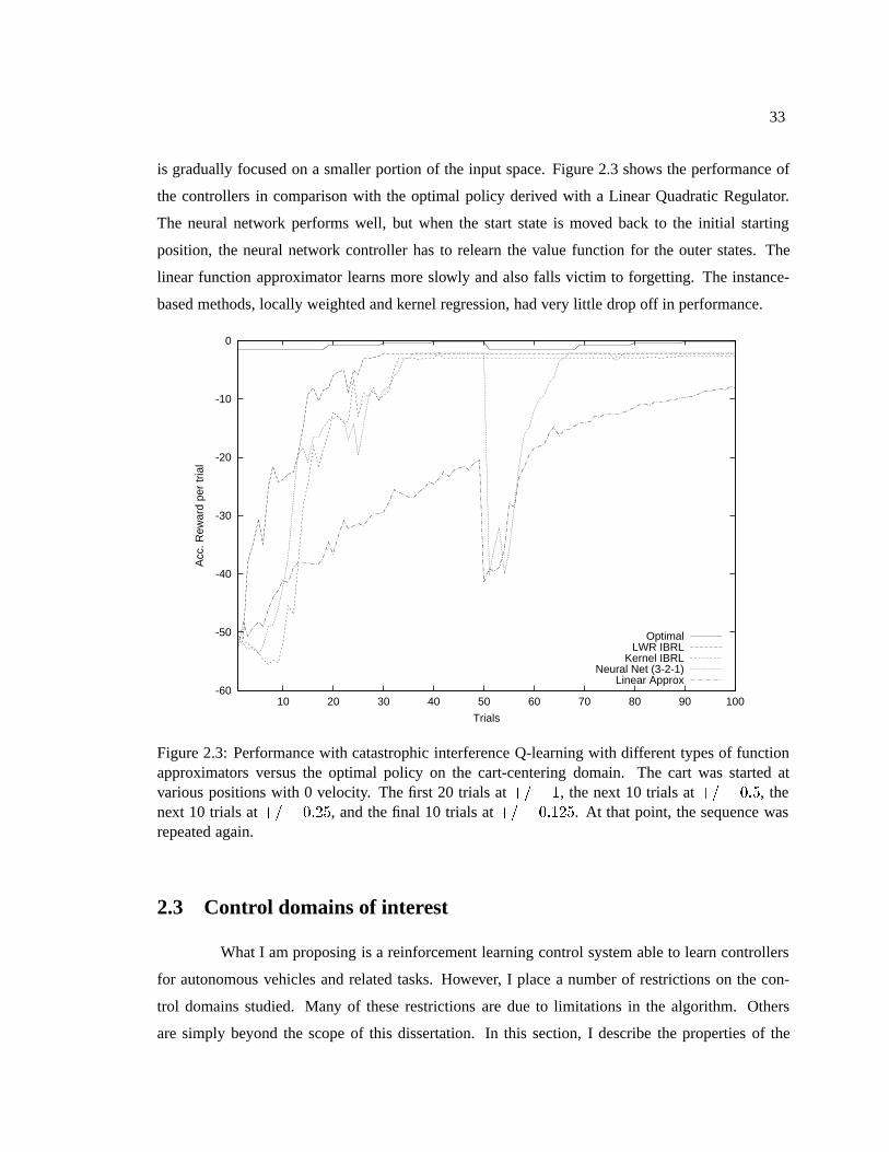
33

is gradually focused on a smaller portion of the input space. Figure 2.3 shows the performance of

the controllers in comparison with the optimal policy derived with a Linear Quadratic Regulator.

The neural network performs well, but when the start state is moved back to the initial starting

position, the neural network controller has to relearn the value function for the outer states. The

linear function approximator learns more slowly and also falls victim to forgetting. The instance-

based methods, locally weighted and kernel regression, had very little drop off in performance.

-60

-50

-40

-30

-20

-10

0

10 20 30 40 50 60 70 80 90 100

Acc

. Rew

ard

per

tria

l

Trials

OptimalLWR IBRL

Kernel IBRLNeural Net (3-2-1)

Linear Approx

Figure 2.3: Performance with catastrophic interference Q-learning with different types of functionapproximators versus the optimal policy on the cart-centering domain. The cart was started atvarious positions with 0 velocity. The first 20 trials at �� , the next 10 trials at �� , thenext 10 trials at �� , and the final 10 trials at �� . At that point, the sequence wasrepeated again.

2.3 Control domains of interest

What I am proposing is a reinforcement learning control system able to learn controllers

for autonomous vehicles and related tasks. However, I place a number of restrictions on the con-

trol domains studied. Many of these restrictions are due to limitations in the algorithm. Others

are simply beyond the scope of this dissertation. In this section, I describe the properties of the

34

control domains of interest. Despite the restrictions below, there are a number of interesting control

problems to be studied:

� Small number � �� of state dimensions: The proposed methods suffer from the curse of

dimensionality, i.e. the number of training examples needed is exponential in the the number

of dimensions of the input space. Most tasks require high accuracy only in small slices of

the input space. As a simple example, for a robot with more than 8 degrees of freedom, it

would be impossible to experience all significantly different configurations in a lifetime, but

any reasonable task would focus on a small part of the space. There has been work done

in dimension reduction where a problem’s input space is projected onto a smaller number

of dimensions [Vijayakumar and Schaal, 2000]. In Chapter 3 and Chapter 6, I revisit the

dimensionality issue. The most important capability of a learning method is to be able to

construct accurate representations of the target representation where there are examples rather

than being able to handle a large number of dimensions.

� Very small number �� of action dimensions: Similarly, the number of action dimen-

sions must also be small, as the action vector is appended onto the state vector to form the

input vector for the function approximation. However, it is especially important that the ac-

tion vector is of extremely small dimensionality. Every policy lookup requires a function

maximization over the action variables. Quickly determining the maximum function with

respect to just one action variable is a nontrivial task. Generally, the number of function

evaluations required to calculate the function’s maximum is exponential in the number of di-

mensions [Gill et al., 1981]. All of the examples I consider have either one or two action

dimensions. That does not restrict the application of methods in the chosen domains. In the

automotive domain, it is reasonable to consider just two sets of actuators, the steering wheel

and the throttle/brake pedal.

� Continuous environment: The work here does not delve into the issues of hybrid control

where there are both discrete and continuous state variables. This limitation might seem

particularly problematic for the driving task. There are a number of relevant discrete percepts.

For example, a neighboring driver’s intentions whether to continue in the same lane or change

lanes to the left or right is a variable with a finite number of distinct states. In cases where

the state variable is discrete and still necessary to our problem, I treat the discrete variable

as continuous anyway. For example, this “lateral intentions” variable described above, would

35

be a real valued variable, valued between -1 and 1. -1 and 1 indicate changing lanes left and

right respectively, while 0 means that the car is continuing to follow its current lane. The

intermediate values are reflective of the probability that the car is changing lanes.

� Fully observable environments: The techniques presented are robust to basic Gaussian

noise as will be seen in Chapter 5, but do not address partial observability. In a partially

observable environment, the agent’s state representation from the sensors will not give an

accurate and complete representation of the relevant traffic state. In order for any system

to show complete proficiency in a realistic or physical environment, the system would have

to be able to accommodate difficulties inherent in partially observable domains. It is use-

ful and still challenging to work in fully observable environments [Crites and Barto, 1996;

Zhang and Dietterich, 1996].

� Markovian environment: The state representation in the environment must not violate the

Markovian assumption. The Markov property holds that the current representation of the state

is all that is needed to determine the evolution of the system. No past history is necessary.

In other words, the future is independent of the past given the present. This Markov property

must hold both in terms of state evolution and in terms of rewards. Without the Markov

property, an accurate value function alone will not guarantee optimal behavior as it would for

a Markov Decision Process.

� Simulatable environment: The task domain needs to be capable of being simulated. The

methods here do not require a mathematical model of the system that can solved, inverted, or

otherwise analyzed. There must be some simulation where we can observe the state transi-

tion and reward models. Given that the number of trials and episodes necessary to become

proficient at most tasks is significant, devising an experiment for a physical system would be

extremely challenging. It is useful for our purposes to plug in new dynamics modules for

a different type of vehicle and induce new controllers without any knowledge of the inner

workings of the vehicle dynamics. In some cases, more complex nonlinear vehicle dynam-

ics may require an augmented state representation. For example, if a model were to include

hills, a 2 dimensional state representation would not accurately model the effect and value of

actions. Increasing the throttle would have drastically different effects on uphill and downhill

segments of road. If our state representation did not include any information about the slope

of the road, the level of perceived stochasticity in the throttle action could be much larger than

36

is reasonable for accurate control. Hidden variables, such as the road slope in this example,

make learning proficient control policies impractical [Lovejoy, 1993].

Beyond the restrictions listed above, I also did not consider some issues out of design.

I only consider single agent learning. My work has not considered the effects of interaction of

learning agents or any implicit or explicit communication between agents. The motivation for this

research is the creation of autonomous vehicles, so I was not concerned with how an autonomous

vehicle interacted with other vehicles with similar controllers. The goal was only to have that vehicle

perform as well as possible according to its performance index. All of the problems I consider are

episodic. Either the agent will fail in some way, or, after some period of time, the agent will be reset

to some initial state. The algorithms would work similarly if the environment was not episodic. The

main reason for having the environment be episodic was because it allowed clear and more precise

simulation and accurate evaluation. It was easier to evaluate an agent on simulations with some

maximum number of steps.

2.4 Problem statement

My thesis is that the instance-based reinforcement learning algorithm described in this

dissertation is a practical and efficient means of learning control of autonomous vehicles.

By practical, I mean that the system developed is easily applied to the domains of interest.

Instead of focusing on asymptotic performance or properties, I focus more on near-term unoptimized

behavior. It remains true that designing a controller for a relatively simple problem such as cart-

centering requires significant expertise in control theory and artificial intelligence. My goal is to

create a system that can learn competent policies for basic control tasks. Competency is often

thought of as a qualitative characteristic. A lane following agent that generally stays within its

lane and reaches the destination is thought of as a competent, while a lane following agent that

spins around on the road is generally considered incompetent. A key first part of competency is

to “stay alive” for the full number of steps in an episode and to perform within some factor of a

baseline controller. The goal is to automatically learn competent systems given little fine-tuning of

the algorithm for a particular domain. I also assume throughout that the agent learns on policy. It

acts and learns at the same time. A practical method must be able to operate continuously without

the performance degrading because of either interference or space limitations. This research yields

the beginnings of a turnkey method for learning optimal control.

37

Related to the practicality of the algorithm is its efficiency. I propose an algorithm suitable

for real-time learning [Forbes and Andre, 2000]. I employ a number of optimizations that enable the

algorithm to handle complex domains without significant fine tuning. Furthermore, it is possible to

trade speed for accuracy by limiting the number of examples stored. Finally, I do not provide tight

bounds on the running times of the algorithms I propose; I do try to ensure that all learning is done

efficiently within an order of magnitude of rule time. Even if the learning is done at a rate ten times

slower than real time, in practice the learning can be moved to a faster computer or implemented on

a parallel system.

2.4.1 Learning in realistic control domains

This dissertation presents a method to efficiently and effectively maintain a value function

estimate using stored instances. The instance-based reinforcement learning algorithm is able to

learn policies for control tasks such as lane following and vehicle tracking. In order to make best

use of learning experience, I present a method that learns a model of the environment and uses

that model to improve the estimate of the value of taking actions in states. I also show how the

learning algorithm can be situated in a hierarchical control architecture to successfully negotiate

driving scenarios.

2.4.2 Current state of the art

While many researchers have noted the applicability of reinforcement learning techniques

to control problems, there have not been general practical solutions for control problems. A gap

between theory and practice remains in applying reinforcement learning in continuous domains.

Moreover, significant applications such as autonomous vehicle control have not been undertaken.

Also novel is the significant application of model-based reinforcement learning in continuous do-

mains.

Instance-based learning has been used frequently in supervised learning. It also has been

used in reinforcement learning [McCallum, 1995; Santamaria et al., 1998; Smart and Kaelbling,

2000; Ormoneit and Sen, 1999]. My contribution is a novel method of maintaining and updating

the value estimate. The values that are stored in reinforcement learning are estimates of the true

expected reward to go. The stored values need to be up updated as more rewards are observed and

the value function approximation becomes more accurate. Updating and maintaining this estimate

on policy is key to being able to learn policies for environments where the example distribution

38

changes and cannot necessarily be controlled. I discuss the similar algorithms in more detail in

Section 3.4.

2.4.3 Discussion

Researchers have discussed and proposed the applicability of reinforcement learning tech-

niques to control problems. Instance-based learning techniques are thought to be particularly well

suited to control problems [Moore et al., 1997]. Few if any have actually succeeded in using re-

inforcement learning to automatically discover reasonable control policies for continuous control

domains. No other reinforcement learning system provides the complete solution, including a ro-

bust value function estimation through instance-based learning (Chapter 3), continuous operation

and managing space restrictions through instance-averaging (Section 3.3.1), and efficient learning

in complex domains due to the use of a learned domain model (Chapter 4). Furthermore, this dis-

sertation presents the reinforcement learning algorithm as part of a larger practical framework for

control of driving (Chapter 5). Not only am I able to learn control for basic “local” tasks such as car

following, but these high-level actions can be used together for an effective driving policy.

A major deficiency in current robotic control techniques is that no systems do significant

online learning [Smart, 2002]. There are systems that adjust some limited set of parameters online,

while others observe information and then do the processing offline. An important goal for my

research is creating systems that will be able to learn online without programmer intervention. In

order to achieve this goal, my controller must be able to handle continual operation and not “forget”

due to interference. Furthermore, the system must be able to learn on policy. The instance-based

reinforcement learning algorithms introduced in this dissertation increase the plausibility of learning

robotic control.

As discussed in Chapter 1, autonomous vehicle control is a problem of significant interest

and impact. Learning techniques have obvious advantages over explicit policy representations for

vehicle control. Learning techniques do not necessarily require a complete model of the system.

Automatically inducing control is clearly useful from an engineer’s perspective as compared to hav-

ing to construct a controller by hand. The decision-theoretic approach of reinforcement learning is

particularly well suited for driving given the often delayed feedback. The instance-based reinforce-

ment learning algorithms presented in this dissertation are a significant contribution to the state of

the art for autonomous vehicle control.

39

2.5 Conclusion

In this chapter, I have laid the framework for later discussion of reinforcement learning

and control. Reinforcement learning is an effective means for controlling complex systems, but,

in order to learn to control an autonomous vehicle from experience, an algorithm must have the

following properties:

� To be able to learn without any prior knowledge of the form of the optimal value function

� To be able to maintain a value estimate when only certain regions of the state space are visited

� To be robust in the presence of catastrophic interference even while the task state distribution

may change over time

� To learn efficiently and reliably from a variety of initial states

I have stated the research problem of learning in continuous, nonstationary control do-

mains. The rest of the dissertation will describe the methods that I have developed for control in

those domains and their performance.

40

Chapter 3

Instance-Based Function Approximation

In Chapter 2, I demonstrated some of the drawbacks of parametric function approxima-

tors. Instance-based techniques have been used effectively for nonparametric learning in a variety

of applications [Aha et al., 1991]. Instance-based learning encompasses a wide range of algorithms,

including nearest-neighbor techniques and memory-based learning. Instead of trying to determine

the shape or distribution of examples a priori, instance-based techniques let the training examples

determine the volume and density of the cells. In control applications, the goal is not necessarily to

most closely model the value function, but to competently control a system. Determining where in

the state space accuracy is most necessary can be difficult, but in this case, the important regions of

the state space are the ones being visited. In driving applications, the distribution of examples tend

to be anything but uniform and constant, as paths may be traversed repeatedly and then rarely visited

again. Many state configurations are unlikely or downright impossible. Instance-based techniques

benefit from being a local approximation method that gives accurate estimates of portions of the

state space even when the majority of the overall space is unvisited.

This chapter describes the instance-based reinforcement learning algorithm. Section 3.1

provides the background on instance-based learning. In Section 3.2, I describe the basic model-free

instance-based reinforcement learning algorithm (IBRL), showing how the results of past experi-

ences can be stored and then used to generalize an estimate of the value of taking actions in states.

Given this basic learning algorithm, Section 3.3 describes a number of necessary extensions that al-

low IBRL to be applied to continuous control problems. Others have used stored instances to learn

control; Section 3.4 describes related work and points out how the work in this dissertation differs.

Section 3.5 then presents the results of applying IBRL to a number of control domains. The results

show that IBRL does efficiently learn control for continuous control tasks.

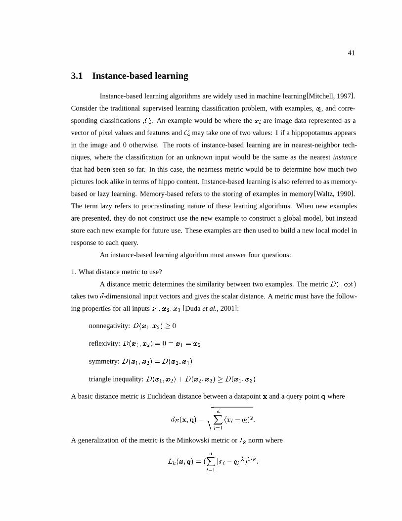
41

3.1 Instance-based learning

Instance-based learning algorithms are widely used in machine learning[Mitchell, 1997].

Consider the traditional supervised learning classification problem, with examples, ��, and corre-

sponding classifications ,,�. An example would be where the �� are image data represented as a

vector of pixel values and features and ,� may take one of two values: 1 if a hippopotamus appears

in the image and 0 otherwise. The roots of instance-based learning are in nearest-neighbor tech-

niques, where the classification for an unknown input would be the same as the nearest instance

that had been seen so far. In this case, the nearness metric would be to determine how much two

pictures look alike in terms of hippo content. Instance-based learning is also referred to as memory-

based or lazy learning. Memory-based refers to the storing of examples in memory[Waltz, 1990].

The term lazy refers to procrastinating nature of these learning algorithms. When new examples

are presented, they do not construct use the new example to construct a global model, but instead

store each new example for future use. These examples are then used to build a new local model in

response to each query.

An instance-based learning algorithm must answer four questions:

1. What distance metric to use?

A distance metric determines the similarity between two examples. The metric -�� "��takes two �-dimensional input vectors and gives the scalar distance. A metric must have the follow-

ing properties for all inputs �� [Duda et al., 2001]:

nonnegativity: -��

reflexivity: -��

symmetry: -�� -��

triangle inequality: -�� -�� -��

A basic distance metric is Euclidean distance between a datapoint � and a query point � where

��

��

�.� � /��

A generalization of the metric is the Minkowski metric or 0� norm where

0��

��

.� � /��

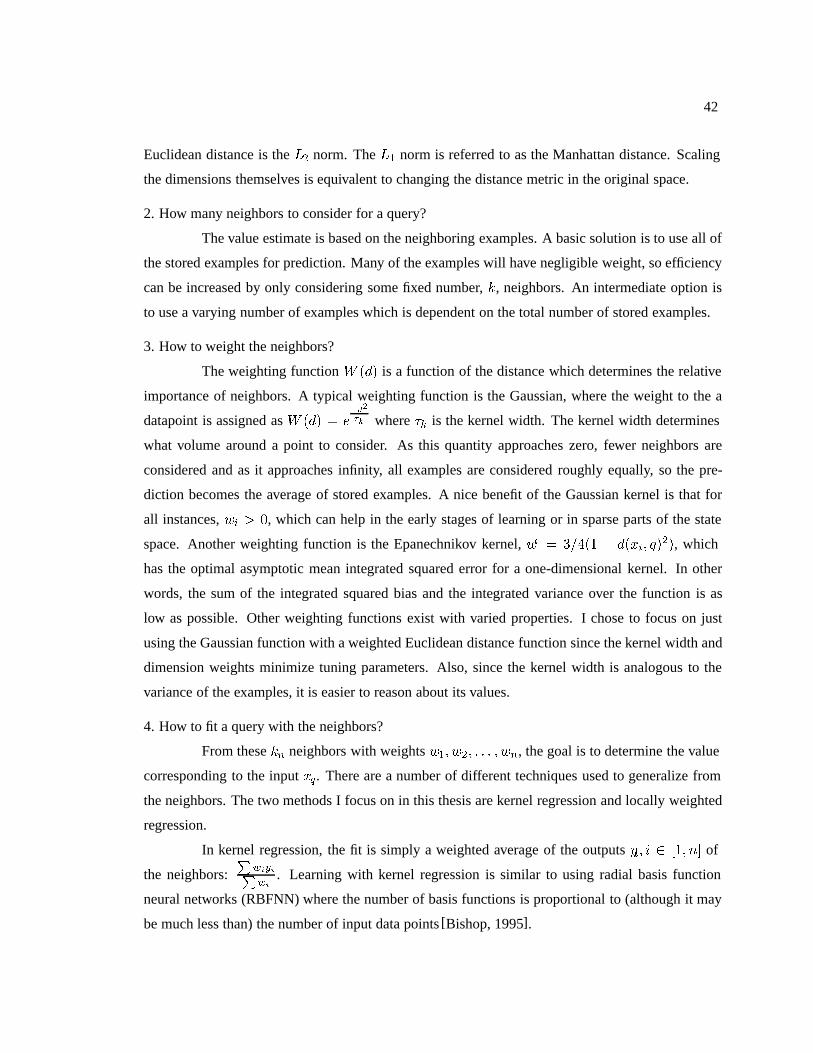
42

Euclidean distance is the 0� norm. The 0� norm is referred to as the Manhattan distance. Scaling

the dimensions themselves is equivalent to changing the distance metric in the original space.

2. How many neighbors to consider for a query?

The value estimate is based on the neighboring examples. A basic solution is to use all of

the stored examples for prediction. Many of the examples will have negligible weight, so efficiency

can be increased by only considering some fixed number, �, neighbors. An intermediate option is

to use a varying number of examples which is dependent on the total number of stored examples.

3. How to weight the neighbors?

The weighting function 1 �� is a function of the distance which determines the relative

importance of neighbors. A typical weighting function is the Gaussian, where the weight to the a

datapoint is assigned as 1 ��

�� where �� is the kernel width. The kernel width determines

what volume around a point to consider. As this quantity approaches zero, fewer neighbors are

considered and as it approaches infinity, all examples are considered roughly equally, so the pre-

diction becomes the average of stored examples. A nice benefit of the Gaussian kernel is that for

all instances, #� � �, which can help in the early stages of learning or in sparse parts of the state

space. Another weighting function is the Epanechnikov kernel, #� � �� .�� /��, which

has the optimal asymptotic mean integrated squared error for a one-dimensional kernel. In other

words, the sum of the integrated squared bias and the integrated variance over the function is as

low as possible. Other weighting functions exist with varied properties. I chose to focus on just

using the Gaussian function with a weighted Euclidean distance function since the kernel width and

dimension weights minimize tuning parameters. Also, since the kernel width is analogous to the

variance of the examples, it is easier to reason about its values.

4. How to fit a query with the neighbors?

From these �� neighbors with weights #�� #�� #�, the goal is to determine the value

corresponding to the input .�. There are a number of different techniques used to generalize from

the neighbors. The two methods I focus on in this thesis are kernel regression and locally weighted

regression.

In kernel regression, the fit is simply a weighted average of the outputs 2�� %� of

the neighbors:�

��

. Learning with kernel regression is similar to using radial basis function

neural networks (RBFNN) where the number of basis functions is proportional to (although it may

be much less than) the number of input data points [Bishop, 1995].

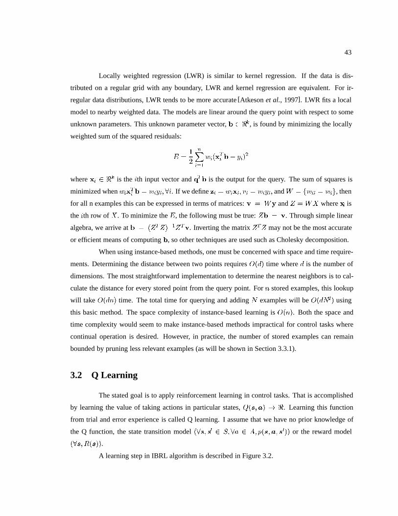
43

Locally weighted regression (LWR) is similar to kernel regression. If the data is dis-

tributed on a regular grid with any boundary, LWR and kernel regression are equivalent. For ir-

regular data distributions, LWR tends to be more accurate [Atkeson et al., 1997]. LWR fits a local

model to nearby weighted data. The models are linear around the query point with respect to some

unknown parameters. This unknown parameter vector, � � ��, is found by minimizing the locally

weighted sum of the squared residuals:

� ��

�

��

#�� 2��

�

where �� is the �th input vector and �� is the output for the query. The sum of squares is

minimized when #�� #�2��. If we define �� #�� #�2�� and1 � �#�� #��, then

for all n examples this can be expressed in terms of matrices: � � 1� and 3 �1* where �� is

the �th row of * . To minimize the �, the following must be true: 3� � �. Through simple linear

algebra, we arrive at � � �3�3��3��. Inverting the matrix 3�3 may not be the most accurate

or efficient means of computing �, so other techniques are used such as Cholesky decomposition.

When using instance-based methods, one must be concerned with space and time require-

ments. Determining the distance between two points requires �� time where � is the number of

dimensions. The most straightforward implementation to determine the nearest neighbors is to cal-

culate the distance for every stored point from the query point. For % stored examples, this lookup

will take ��%� time. The total time for querying and adding 4 examples will be ��4�� using

this basic method. The space complexity of instance-based learning is ��%�. Both the space and

time complexity would seem to make instance-based methods impractical for control tasks where

continual operation is desired. However, in practice, the number of stored examples can remain

bounded by pruning less relevant examples (as will be shown in Section 3.3.1).

3.2 Q Learning

The stated goal is to apply reinforcement learning in control tasks. That is accomplished

by learning the value of taking actions in particular states, �� . Learning this function

from trial and error experience is called Q learning. I assume that we have no prior knowledge of

the Q function, the state transition model �� or the reward model

�� .A learning step in IBRL algorithm is described in Figure 3.2.

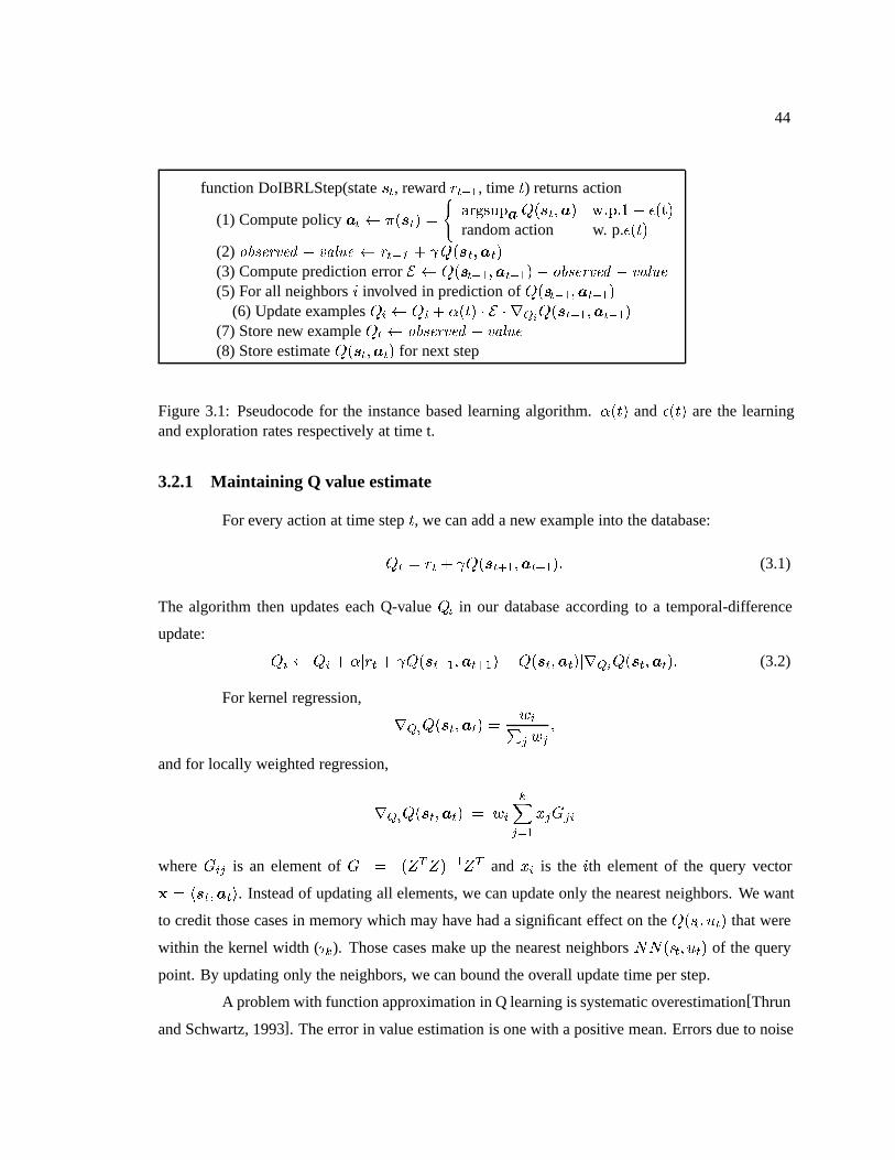
44

function DoIBRLStep(state ��, reward ��, time �) returns action

(1) Compute policy ��

�� $��random action w. p.$��

(2) �� (3) Compute prediction error � ��

(5) For all neighbors � involved in prediction of ��(6) Update examples ��

��(7) Store new example ��

(8) Store estimate �� for next step

Figure 3.1: Pseudocode for the instance based learning algorithm. �� and $�� are the learningand exploration rates respectively at time t.

3.2.1 Maintaining Q value estimate

For every action at time step �, we can add a new example into the database:

�� (3.1)

The algorithm then updates each Q-value �� in our database according to a temporal-difference

update:

�� (3.2)

For kernel regression,

��

#�� #�

�

and for locally weighted regression,

�� #�

��

.�5��

where 5�� is an element of 5 � �3�3��3� and .� is the �th element of the query vector

� � ��. Instead of updating all elements, we can update only the nearest neighbors. We want

to credit those cases in memory which may have had a significant effect on the �� !�� that were

within the kernel width (��). Those cases make up the nearest neighbors 44�� !�� of the query

point. By updating only the neighbors, we can bound the overall update time per step.

A problem with function approximation in Q learning is systematic overestimation[Thrun

and Schwartz, 1993]. The error in value estimation is one with a positive mean. Errors due to noise

45

may be either positive or negative, but since only the highest Q values are propagated in the policy

updates, the positive errors spread. Unfortunately, this overestimation has a more significant effect

on continuous control domains where many of the actions have similar values. The number of “good

moves” is infinite, since the actions are continuously varying. That makes domains with continuous

actions more susceptible to overestimation.

3.2.2 Calculating the policy

Given an accurate estimate of the Q function, one can calculate the optimal action � in

any state � according to the policy defined as �� . Note that we have an

�� to compute instead of an �� , since we are now dealing with a continuous action

vector. Finding the maximum value for an arbitrary function can be a complex exercise in itself.

Many algorithms discretize the action space, but for many control tasks, too coarse a discretization

of actions can cause oscillations and unstable policies[Kumar and Varaiya, 1986]. One simplifying

assumption is that there is a unimodal distribution for the Q-values with respect to a particular state

and scalar actions. While the underlying distribution may be unimodal, the Q function estimate is

often quite “bumpy” with many local minima. In fact, each example represents another “bump”

when using instance-based techniques because the estimate always depends heavily on the nearest

neighbor. The weighting function will smooth out the Q estimate, but finding the maximum Q value

for a particular state may still be difficult. Avoiding suboptimal actions in a continuous action space

may be impossible, but by conducting a beam search where there are multiple parallel searches each

returning a maximum, the optimization does well. The estimate of the global maximum is then the

best of these searches. Each beam search uses a gradient ascent strategy to find a locally optimal

action for our value function. As the number of beam searches approaches infinity, the maximum

returned approaches the global maximum. In practice, of course, a large or unbounded number of

searches cannot be performed on every policy lookup.

Moreover, calculating the policy is done at each step and must be as efficient as possible.

Care must be taken in choosing a function maximization technique because repeated evaluations of

the function approximator can be expensive. Calculating the derivative of the function also proves

to be difficult because it generally requires repeated applications of the function to determine the

empirical derivative estimate. An effective technique is to use Brent’s Method, where the algorithm

fits a parabola to the function and then uses that to jump close to the maximum in fewer steps[Brent,

1973].

46

In domains where the action is represented by a vector instead of a single scalar value,

the maximum finding routine is accordingly more complex. It becomes difficult to fit a parabola

here. The first step is to try to limit the number of dimensions in the action vector. After that, we

use simulated annealing to find the maximum [Kirkpatrick et al., 1983]. Simulated annealing is a

gradient ascent method where random moves “down the hill” are occasionally chosen according to

an annealing schedule to keep from being stuck in local maxima. The number of evaluations re-

quired to find a maximum increases exponentially with the number of action dimensions. Baird and

Klopf’s optimization algorithm [Baird and Klopf, 1993], wire fitting, fits the function to be maxi-

mized with a set of curves called control wires. Control wires are constructed from the examples

so that the function is fitted to control curves. Each new example creates a curve and the maximum

is just the maximum curve at any point. Wire fitting can be used instead of instance-based learning

for Q function approximation but there has been little success using it in practice. Nevertheless, the

general idea of storing the function as a set of control points in order to find the maximum quickly

has promise and may be the subject of future inquiry.

It is not enough, however, to follow the policy described above taking the action pre-

scribed by the value function at every step. In order for the agent to “experience” all parts of the

state space, the agent must explore the state space. Otherwise, the agent could converge to some

unacceptable but locally optimal policy. In the case of lane following, there are many classes of

suboptimal policies that do not yield the desired behavior of following the lane. Spinning around

on a road may be a locally optimal policy when compared to policies where the vehicle ends up

driving off the road. The accumulated reward for a policy where a car spins on the road should be

less than that of a car which drives down the road to its destination following the lane all along the

way. However, if an agent stumbles upon the the “spin” policy, it may never find out that driving

down the road is an option. The agent has no knowledge of rewards or penalties existing in parts

of the state space it has not seen. Only after visiting all states an infinite number of times can the

agent know the actual optimal policy. In constructing a policy, one is presented with the exploration-

exploitation dilemma. The agent can either exploit its current knowledge, its value estimate, or it

can explore in order to improve the accuracy and completeness of its value estimate to make better

decisions in the future. This dilemma for years has been a subject of study by mathematicians and

statisticians [Berry and Fristedt, 1985].

Despite the challenges of action selection mentioned here, the system does learn to choose

suitable actions for the control domains. Through some experimentation and inquiry, develop-

ing policies proved to be workable. The approximations made by the optimization schemes and

47

the careful selection of state features make constructing a policy from the function approximation

achievable.

3.3 Extensions

The basic idea of using instance-based methods for value function approximation is crit-

ical to being able to effectively learn controllers, but extensions are necessary to maintain a value

function estimate in continual operation in domains. Simple instance-based learning alone will not

be able to be a practical method for control of autonomous vehicles. The number of stored examples

would become unmanageable as the agent continued to learn. Also, nearest neighbor techniques are

sensitive to the relative values and variances of the different state vector dimensions. For proper

generalization, extensions have to be be made to adapt to the relative importance and range of the

different features.

3.3.1 Managing the number of stored examples

For the applications that have been discussed, the system may need to continue to operate

and learn for an arbitrary length of time. While there do exist some well-practiced techniques for

pruning “useless” examples in training [Bradshaw, 1985; Kibler and Aha, 1988; Kohonen, 1990],

learning in this setting poses a few more difficulties. One method of editing the set of examples is

to determine if an example contributes to a decision boundary. If one of its neighbors has a different

value then it remains in the set, otherwise it is removed. This algorithm can reduce the number of

examples with no effect on the algorithm’s accuracy. However, for a number of reasons, this method

does not work for value function approximation. First, this task is not one of classification but of

regression, so there are no decision boundaries. Instead, there are gradations of value in regions,

and it is unknown how finely-grained those gradations may be. Also this editing method requires

knowledge of all the training data ahead of time. Once all examples have been seen, it is possible to

rule out that a particular region, no matter how small, could have a completely different value than

the points around it. An online algorithm has to determine the complexity of value space as new

states and rewards are experienced.

Finally, the stored examples are only estimates, so it is not possible to know whether an

example is an important outlier or just wrong. If the example bound is set too low, the estimates

may not be good enough to warrant trying to determine which ones are most essential. Premature

48

pruning is particularly harmful for reinforcement learning where it may take a number of trials

before a goal is even reached and any useful feedback is gained. While it may not be possible to

find a pruning algorithm that reduces space and time requirements without compromising accuracy,

we can pick examples to prune that appear to have the least effect on the estimate.

A first step in managing the size of the examples set is to limits its growth; redundant

examples should not be added. There is a density parameter, ��, that limits the density of examples

stored. For every new example, ��, if ��-�� , then �� is added to the set of examples.

Since the neighboring examples will be updated, the effect of the new experience will still be incor-

porated into the overall estimate. Another optimization is to add only those examples that cannot

be predicted within some parameter $. Both �� and $ can be adjusted down to increase accuracy or

up to decrease memory requirements. While these optimizations can have both direct and indirect

effects on the learning process, they are useful in practice in limiting the growth of the example set.

Being selective in adding examples may slow growth; but when the number of examples is greater

than the maximum number allowed, some example must be removed. A first approach would be to

remove the oldest example. Another possibility would be to remove the least recently “used” exam-

ple, the example that has not been a neighbor in a query for the longest time. There are problems

encountered with these methods that are similar to those using a parametric function approximator,

namely in the forgetting experiences from the past. This forgetting can be particularly problematic

if some important experiences only occur rarely, though, in some cases, forgetting early experiences

can be beneficial, since early estimates often provide no useful information and can be misleading.

Forgetting the most temporally distant examples does not differentiate between incorrect examples

and relevant old examples.

Instead of removing old examples, the examples that should be removed are those that

contribute the least to the overall approximation. The example that is classified the best by its

neighbors, and where the neighbors can still be classified well or possibly better without the exam-

ple, should be chosen for averaging. The score for each exemplar, �� can be computed as follows:

�"��

�

��

��

where �� is the the evaluation of the Q function at �� while not using �� in the

evaluation. The scores can be updated incrementally in the time it takes for a Q evaluation. Instead

of removing the example with lowest score, a better method is instance-averaging – where two

neighbors are reduced into one exemplar, which is located at the midpoint of the two inputs and its

value is the mean of the two values. Averaging reduces the bias in comparison to just removing

49

an example. A similar approach was proposed by Salzberg where instead of averaging instances,

he generalizes instances into nested hyperrectangles [Salzberg, 1991]. While partitioning the space

into hyperrectangles can work well for discrete classification tasks, it has flaws for regression. Most

importantly, all of the points within a region almost never have the exact same value. In general, we

only care about the highest Q-value for a particular state and thus we can sacrifice precision for the

values of suboptimal actions. If a domain model is used, then it is possible instead to store the value

function, � ��. The value function does not save the values of suboptimal actions. An interesting

future direction would be to design a heuristic for instance-averaging which takes into account the

reduced utility of suboptimal Q values for a particular state.

3.3.2 Determining the relevance of neighboring examples

Each estimate is computed from the values of its neighbors. The estimate is sensitive to

distances between examples in the input space and to how much each of the examples is weighted.

The kernel size and the number of neighbors determine the size of the relevant neighborhood. The

different dimensions in a input vector tend to have different levels of importance.

Kernel size

The kernel width �� determines the breadth of influence for each example. Selecting a

kernel width can be crucial to the agent’s learning performance. A kernel width that is set too

small will result in poor generalization performance, since anything that has not been previously

experienced will remain unknown. A kernel width that is too high results in low accuracy, as

all examples will be considered equally for all queries. The effect would be that the estimator

would return only the average of all stored examples. There has been work in finding the optimal

kernel width for supervised learning. Fan and Gijbels derive a formula for optimal variable kernel

bandwidth [Fan and Gijbels, 1992] which requires multiple passes through all of the data.

A key insight is that the kernel width should depend on the mean distance between neigh-

bors. As the examples become more bunched, then the kernel width should decrease. A similar

means of maintaining accuracy is to only use some fixed number of neighbors as discussed above.

Dimension weighting

It is often desirable to scale and skew the input space so that more attention is paid to

certain dimensions in the distance metric. This effect is achieved by adding a covariance matrix to

50

the Gaussian weighting function. Thus, for two points .� 2 in state,action� space, we use

#�.� 2� � ��

#�� is a matrix that is essentially the inverse covariance matrix of the Gaussian. Note that a single

#�� is used for all the data. Thus, when Q is updated, #�� must also be updated. This update is

shown below:

#��

��

Beyond dimension weighting, some dimensions may be irrelevant altogether.

3.3.3 Optimizations

As this work is motivated by working on autonomous vehicles, the instance-based rein-

forcement learning algorithm must be as efficient as possible. Furthermore, it is important that the

learning steps can be done in close to real time. A previous paper discusses the reinforcement learn-

ing system in terms of its abilities to be a real-time autonomous system[Forbes and Andre, 2000].

As with most learning tasks, the goal is to reach a certain level of performance in as few training

steps as possible. I have already mentioned in Section 3.3.1 that bounding the number of examples

limits the time of the value computation and updating steps will take. However, efficiency of the

system allows for maximization of the number of examples that can be stored and the speed with

which the system learns.

Determining the k nearest neighbors of an example can be achieved more efficiently using

kd-trees [Moore, 1991]. A kd-tree is a binary tree data structure for storing data points in a �

dimensional space. Levels of the tree are split along successive dimensions at the points. Lookup

of neighbors is significantly faster using kd-trees. If the number of neighbors is 4 and the total

number of examples is %, on average the lookup time will be proportional to 4 ��%.

The number of input dimensions is a key contributor to the performance of IBRL. By

projecting from the original input space to one with a smaller number of dimensions, the individual

learning steps will be faster, since the distance calculations will take less time. The kd-tree lookup

time will also be less. There are a number of techniques for projecting an input space onto some

smaller number of dimensions by focusing on the redundancy in the data. Most control systems can

generally be formulated using a smaller number of dimensions.

51

3.4 Related Work

There has been significant research in using instance-based learning for control. Most of

the work focuses on learning direct input-output mappings for control tasks. Moore, Atkeson, and

Schaal and show that techniques that store examples are ideally suited for control [Moore et al.,

1997]. In particular, they focus on a method of generalization called locally-weighted regression

which has good properties for estimation. They show how instance-based learning can be used for

supervised learning of control. They propose that instance-based learning would be useful as a value

function approximation method in reinforcement learning. In fact, the algorithms in this thesis are

motivated by many of the suitable properties of instance-based learning techniques for control put

forth by the authors:

� Builds a locally linear model from the data that can represent globally nonlinear functions

� Incorporates new data into model efficiently since instance-based learning is lazy and does

not construct a global model

� Is suitable for online learning because of “one-shot learning” where multiple passes over the

data are not necessary

� Enables efficient searches for model parameters because of cheap cross validation

� Benefits from from well known properties and a wide body of statistical literature on non-

parametric function approximators

� Avoids interference

Researchers have successfully extended locally weighted learning for control. Schaal and

Atkeson [Atkeson and Schaal, 1997; Schaal and Atkeson, 1998] use locally weighted regression

to learn to control a robot arm doing tasks such as pole balancing and “devil sticking.” The sys-

tems would “learn from demonstration.” Their algorithm, Receptive Field Weighted Regression

(RFWR), enriches the models for the individual instances. Instead of each instance storing a value,

the instances are receptive fields that perform individual locally weighted regression based on the

data. The predicted values from the different receptive fields are then combined in a weighted aver-

age to arrive at the overall prediction. In order to handle higher dimensional input spaces, Schaal,

Atkeson, and Vijaykumar developed Locally Weighted Projection Regression (LWPR) where each

52

input is projected down onto a smaller number of dimensions by each receptive fields. The regres-

sion is done in a smaller number of dimensions. Clearly, the complexity of each example increases

and my efforts to use RFWR and LWPR for function approximation did not have practical results

at this time, but the technique does have significant promise for RL with optimizations.

Instance-based learning has also been used for function approximation in reinforcement

learning. Andrew McCallum’s thesis uses instance-based function learning to resolve hidden state.

The learner is used in utile-distinction trees that stored the reward-history of the system so a value

function tree could be built over a subset of the environment features.

The work of Santamaria, Sutton, and Ram provided much of the inspiration for the

instance-based reinforcement learning algorithm described in this chapter[Santamaria et al., 1998].

The authors apply a number of value function approximation techniques to online learning of control

tasks. They use Cerebellar model articulation controller, instance-based, and case-based function

approximators. Their instance-based approximator is similar to the kernel regression presented here

in Section 3.1. The examples in a case-based approximator add more data to the state-action pair

in the input about previously visited states. The learning algorithms were applied to cart centering

and pole balancing. The contribution this dissertation makes is in presenting the general update

rule for instance-based approximators presented in Equation 3.2. Furthermore, this dissertation ad-

dresses many of the practical problems that come up when applying reinforcement learning to more

complex problems such as vehicle control. In particular, my work addresses limited space and time

resources

Another similar line of research is that of Ormoneit and Sen [Ormoneit and Sen, 1999].

They present an algorithm called kernel-based reinforcement learning which has both practical and

theoretical promise. This algorithm converges to the optimal solution of the Bellman equation

shown in Equation 2.28. Given a set of state transitions, $ � �� for � � �� where

� is the number of steps and $� � �� being a collection of transitions where action �

was taken, kernel-based reinforcement learning applies a Q-update on all transitions for a particular

action, $�. An interesting result is that kernel regression when used as function approximation

technique performs like an averager which does converge to a unique fixed point[Gordon, 1995].

The algorithm relies on there being a finite number of actions in order for it to be feasible, since

the value is estimated by averaging the values of estimates of previous times when the action was

executed in similar states. In control domains, there is an infinite number of actions that necessitate

an incremental approach.

53

A similar method to the one in this dissertation is that of Smart and Kaelbling[Smart and

Kaelbling, 2000]. Our approaches were developed independently [Forbes and Andre, 1999], and

both approaches were motivated by the goal of making reinforcement learning practical for dynamic

control tasks. Smart and Kaelbling do not mention the general update rule I develop here. Their

approach focuses on developing methods for robotic control. One particularly impressive aspect of

their work is that given some bootstrapping by watching a somewhat competent human at a task,

the system learns quickly and exceeds the human performance.

All of this related work by other authors indicates that reinforcement learning using

instance-based methods for function approximation is a theoretically and empirically well founded

solution for control. In Chapter 6, I discuss how this research and the others mentioned above can

be integrated into my own work.

3.5 Results

The pole balancing or cart-pole problem is among the most common control domains. A

pole is anchored to a cart which is on a one dimensional track. The pole is subject to gravity causing

it to fall to one side or the other. By moving the cart form side to side, the pole will remain upright.

The state of the system is a 4 dimensional vector with the cart’s position � and velocity �� and the

pole’s angle 6 and angular velocity �6. The action is the force applied on the cart. The goal is to keep

the pole upright with negligible angular velocity and negligible translational velocity for the cart.

The reward function is:

��

�� 6� � �6�� 6 ��

�� 7�8��#��(3.3)

The results of learning are in Figure 3.2. Once again, IBRL learns the task quicker and

more stably than using the generic linear function approximator.

Thus far, I have not discussed the convergence properties of this algorithm. In practice,

the algorithm does not always converge to a reasonable policy. This suboptimal behavior occurs

for two reasons. One problem is that learning on policy means that the example distribution is

directly tied to the policy. A “bad” policy may lead to more bad examples without ever venturing

into the “good” region of the example space. It is important that the exploration rate not decrease

too quickly, else initial value estimates become too influential. If the exploration rate decreases

too quickly or initial learning is otherwise misleading, the system may converge to a poor set of

54

htb

-120

-100

-80

-60

-40

-20

0

0 200 400 600 800 1000 1200 1400 1600 1800 2000

Acc

. Rew

ard

per

tria

l

Trial

IBRLLinear Approx

Figure 3.2: Pictured is the accumulated reward per trial for the cart-centering domain. The compar-ison is between the reinforcement learning using instance-based and linear function approximators.Each trial has a maximum length of 100 steps

55

policies and never experience the more fruitful regions of the state-action space. The other cause of

problems is that the features must be chosen carefully. Dimension weighting helps in determining

which features appear to have a greater contribution to value, but sometimes dimension weighting

can exacerbate the problem. Also, if the number of dimensions in the example space becomes large,

exploring the space becomes even more difficult.

Nevertheless, there are results suggesting that the algorithm should have good conver-

gence properties. Ormoneit and Sen show how kernel-based reinforcement learning converges to

a fixed policy for a finite number of states and actions. While these do not apply for continuous

domains, they do confirm that the instance-based function approximation method is well founded.

3.6 Conclusion

This chapter described an instance-based reinforcement learning algorithm for continuous

state spaces. I demonstrated a mechanism for maintaining the Q-function estimate using instance-

based function approximators, and have shown the results of applying the technique to control

domains. Furthermore, I have shown, both empirically and theoretically, that parametric function

approximators suffer from the forgetting problem. Also, I described a method for limiting the

amount of stored data. In Chapter 4, I describe how to use the instance-based Q-value estimate for

model-based reinforcement learning. In Chapter 6, I will discuss other domains where I will apply

this technique as well as ways of extending the instance-based methods to support other kinds of

prediction methods.

56

Chapter 4

Using Domain Models

4.1 Introduction

Despite significant progress in theoretical and practical results for reinforcement learn-

ing, RL algorithms have not been applied on-line to solve many complex problems. One reason is

that the algorithms are weak learning algorithms in an AI sense. They use a tabula rasa approach

with little or no prior domain knowledge and will generally scale poorly to complex tasks[Mataric,

1991]. However, there are model-based approaches which can incorporate domain knowledge into

directing the search of a RL agent. The algorithms use experience to build a model, use the expe-

rience to adjust the estimated utility of states, and then use that model and the utility function to

update the policy.

As is well known in the reinforcement learning community, a model of the environment

can be used to perform extra simulated steps in the environment, allowing for additional planning

steps [Sutton, 1990]. In the extreme, the MDP in question could be solved as well as possible given

the current model at each step. For the problems of interest here, this approach is intractable, and

certainly undesirable when the model is not very accurate. Thus, most applications benefit from a

middle ground of doing some extra planning steps after each actual step in the environment. The

technique of Prioritized Sweeping [Moore and Atkeson, 1993] chooses the states to update based on

a priority metric that approximates the expected size of the update for each state. In this work, the

principles of generalized prioritized sweeping[Andre et al., 1997] are applied to a continuous state

and action space using an instance-based value-function and a dynamic Bayesian network (DBN)

representation of the model. A potential disadvantage of using a model is that it must be learned,

which can be difficult in a complex environment. However, by using a simple DBN for the model,

57

one can take advantage of prior knowledge about the structure of the environment, and are left only

with the problem of learning the parameters of the DBN.

4.2 Using a domain model

Most control architectures can be characterized as either direct or indirect. Indirect con-

trollers use a model of the environment in constructing the policy, while direct controllers optimize

the policy directly and use no explicit model of the environment. In the control literature, the process

of forming a model of an agent’s environment is called system identification. System identification

can be done either off-line, by learning an environment model from system traces or on-line while

exploring and learning in the environment. Model-based RL is a form of indirect control with on-

line identification. A problem that arises when using models is that one must solve the problem of

learning a model and learning control at the same time. The difficulties of solving both problems

has been studied since the 1960s and is often referred to as the dual control problem[Feldbaum,

1965].

The standard problem in model-based reinforcement learning is to learn a model of the

environment simultaneously with an optimal policy. As the agent gains knowledge of the world’s

model, this information can be used to do various forms of planning, which can update the agent’s

value function without taking steps in the world. In the ideal case, the agent would compute the

optimal value function for its model of the environment each time it updates it. This scheme is

unrealistic since finding the optimal policy for a given model is computationally non-trivial. This

scheme can be approximated by noticing that the approximate model changes only slightly at each

step. The value function from the previous model can be easily “repaired” to reflect these changes.

This approach was pursued in the DYNA [Sutton, 1990] framework, where after the execution

of an action, the agent updates its model of the environment, and then performs some bounded

number of value propagation steps to update its approximation of the value function. Each value-

propagation step in the standard model-based framework locally enforces the Bellman equation by

setting %� �� %�� where %�� %��

��

�� %� ��, where �� and

%�� are the agent’s approximate model, and %� is the agent’s approximation of the value function.

In the SARSA framework [Singh and Sutton, 1996] utilized here, simulated value propagation steps

are performed by taking simulated steps in the environment, using the learned model. To do a value

propagation for a state-action pair �� , simulate the action �� using the model, and

calculate the resultant state �� , and then pick an action �� , and calculate its value �� . Then,

58

the value of �� can be updated as follows: �� .

4.2.1 Structured models

In a discrete state space, it is possible to store the model simply as a table of transition

probabilities. Clearly, in a continuous domain, other forms of representation are required. One

possibility is to use use an instance-based function approximator as in Chapter 3. Instance-based

learning has been successful in learning models of dynamical systems from scratch[Moore et al.,

1997]. However, if the basic structure of the environment is known, learning a structured para-

metric model can be more effective. By using the known structure of the environment, learning the

model can be done more efficiently, since it becomes a problem of parameter estimation. Moore and

Atkeson used a simple constrained parametric model of a robot arm in their learning from obser-

vation research [Atkeson and Schaal, 1997]. Other researchers in robotics have used Kalman-filter

style models for navigation under uncertainty. In any complex reinforcement learning environment,

however, there are often many state variables, and the transition matrices for a Kalman-filter might

become unwieldy. The curse of dimensionality can be sidestepped by using a model that takes

advantage of local structure.

Dynamic Bayesian networks

One particular compact representation of �� is based on dynamic Bayesian net-

works (DBNs)[Dean and Kanazawa, 1989]. DBNs have gone by several other names as well, in-

cluding Dynamic Probabilistic Networks or Dynamic Belief Networks. DBNs have been combined

with reinforcement learning before [Tadepalli and Ok, 1996], where they were used primarily as a

means of reducing the effort required to learn an accurate model for a discrete world.[Andre et al.,

1997] also used DBNs in their work on extending prioritized sweeping.

I start by assuming that the environment state is described by a set of attributes. Let

�� be random variables that describe the values of these attributes. For now, I will assume

that these attributes are continuous variables, with a predefined range. An assignment of values

�� to these variables describes a particular environment state. Similarly, I assume that the

agent’s action is described by a random variable ��. To model the system dynamics, I have to

represent the probability of transitions � ��, where � and � are two assignments to �� and

� is an assignment to ��. To simplify the discussion, I denote by 9�� 9� the agent’s state after

the action is executed (e.g. the state �). Thus, �� is represented as a conditional probability

59

density function ��9�� 9� �� .

A DBN model for such a conditional distribution consists of two components. The first

is a directed acyclic graph where each vertex is labeled by a random variable and in which the ver-

tices labeled *�� *� and �� are roots. This graph specifies the factorization of the conditional

distribution:

� �9�� 9� ��

��

� �9� :��

where :�� are the parents of 9� in the graph. The second component of the DBN model is a

description of the conditional probabilities � �9� :��. Together, these two components describe

a unique conditional distribution. In the case of discrete variables, the simplest representation of

� �9� :�� is a simple table. The use of continuous variables requires a parameterized function to

specify the conditional probabilities. In this case, I use a constrained form of the exponential family

where the function � �9� :�� is represented by a Gaussian (normal) distribution with a mean

that is a linear combination over a set of functions on the inputs, and a variance over the same set

of functions. That is, �9� :�� 6�;�:�� <��, where ;�:�� is a set of functions over the

parents of the given state attribute. For example, a node that was such a function of two parents *�

and *� might have the form: � ��6� � 6�*� � 6�*� � 6�*�*�� <��.

It is easy to see that the “density” of the DBN graph determines the number of parameters

needed. In particular, a complete graph requires ��4�� parameters, whereas a sparse graph requires

��4� parameters.

I assume that the learner is supplied with the DBN structure and the form of the sufficient

statistics (the ;�:��)) for each node, and only has to learn the 6�� , where � indexes the node 9� and

= the =th parameter of node 9�. The structure of the model is often easy to assess from an expert.

Friedman and Goldszmidt [Friedman and Goldszmidt, 1998] describe a method for learning the

structure of DBNs that could be used to provide this knowledge.

Assuming a fully observable environment, learning the parameters for such a model is

a relatively straightforward application of multi-variate linear regression. For the purposes of this

dissertation, I assume a constant variance, although clearly this could be learned through experience

using stochastic gradient or other related techniques. Without the need to learn the variance of the

function at each node, one can simply determine the linear coefficients for each equation. Keeping

track of the values of the sufficient statistics , the coefficients can be learned online at each node by

solving a simple system of equations equal in size to the number of parameters (that can be derived

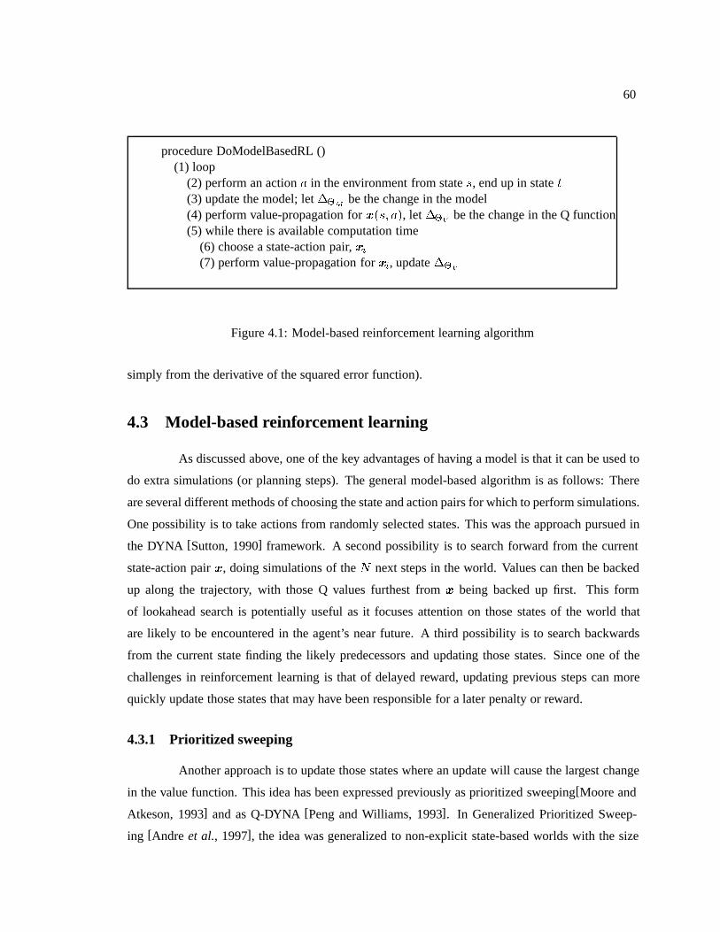
60

procedure DoModelBasedRL ()(1) loop

(2) perform an action � in the environment from state �, end up in state �(3) update the model; let ��

be the change in the model(4) perform value-propagation for �� , let ��

be the change in the Q function(5) while there is available computation time

(6) choose a state-action pair, ��(7) perform value-propagation for ��, update ��

Figure 4.1: Model-based reinforcement learning algorithm

simply from the derivative of the squared error function).

4.3 Model-based reinforcement learning

As discussed above, one of the key advantages of having a model is that it can be used to

do extra simulations (or planning steps). The general model-based algorithm is as follows: There

are several different methods of choosing the state and action pairs for which to perform simulations.

One possibility is to take actions from randomly selected states. This was the approach pursued in

the DYNA [Sutton, 1990] framework. A second possibility is to search forward from the current

state-action pair �, doing simulations of the 4 next steps in the world. Values can then be backed

up along the trajectory, with those Q values furthest from � being backed up first. This form

of lookahead search is potentially useful as it focuses attention on those states of the world that

are likely to be encountered in the agent’s near future. A third possibility is to search backwards

from the current state finding the likely predecessors and updating those states. Since one of the

challenges in reinforcement learning is that of delayed reward, updating previous steps can more

quickly update those states that may have been responsible for a later penalty or reward.

4.3.1 Prioritized sweeping

Another approach is to update those states where an update will cause the largest change

in the value function. This idea has been expressed previously as prioritized sweeping[Moore and

Atkeson, 1993] and as Q-DYNA [Peng and Williams, 1993]. In Generalized Prioritized Sweep-

ing [Andre et al., 1997], the idea was generalized to non-explicit state-based worlds with the size

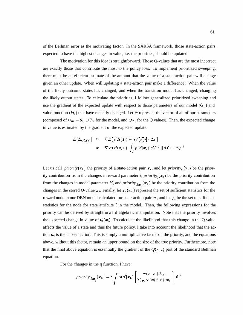
61

of the Bellman error as the motivating factor. In the SARSA framework, those state-action pairs

expected to have the highest changes in value, i.e. the priorities, should be updated.

The motivation for this idea is straightforward. Those Q-values that are the most incorrect

are exactly those that contribute the most to the policy loss. To implement prioritized sweeping,

there must be an efficient estimate of the amount that the value of a state-action pair will change

given an other update. When will updating a state-action pair make a difference? When the value

of the likely outcome states has changed, and when the transition model has changed, changing

the likely output states. To calculate the priorities, I follow generalized prioritized sweeping and

use the gradient of the expected update with respect to those parameters of our model (& ) and

value function (&�) that have recently changed. Let & represent the vector of all of our parameters

(composed of & � 6�� 6�� for the model, and ��for the Q values). Then, the expected change

in value is estimated by the gradient of the expected update.

�� %� ��

�� %� ��

Let us call priority�� the priority of a state-action pair ��, and let priority�� be the prior-

ity contribution from the changes in reward parameter �, priority�� be the priority contribution

from the changes in model parameter �=, and priority�� be the priority contribution from the

changes in the stored Q-value �� . Finally, let ;�� represent the set of sufficient statistics for the

reward node in our DBN model calculated for state-action pair ��, and let ;� be the set of sufficient

statistics for the node for state attribute � in the model. Then, the following expressions for the

priority can be derived by straightforward algebraic manipulation. Note that the priority involves

the expected change in value of ��. To calculate the likelihood that this change in the Q value

affects the value of a state and thus the future policy, I take into account the likelihood that the ac-

tion �� is the chosen action. This is simply a multiplicative factor on the priority, and the equations

above, without this factor, remain an upper bound on the size of the true priority. Furthermore, note

that the final above equation is essentially the gradient of the �� part of the standard Bellman

equation.

For the changes in the q function, I have:

priority��

��

��

��

�� %��

��

62

where �� ranges over the set of possible outcomes from state-action pair ��, and %� is the best action

from state ��. For the changes in the model, the associated priority is:

priority�� ;��

priority��

��'��

�� 6��;��;��

��

4.3.2 Efficiently calculating priorities

Now there is, of course, a problem with the above equations. The integrals must be evalu-

ated. In practice, that can be done by sampling, but care must be taken to insure that the calculation

of priorities remains a cheap operation in comparison with the cost of doing a value update – other-

wise it would be advisable to spend time on extra random updates, rather than on calculating prior-

ities. To get around this problem, the following approximation can be used: ��%� �� %� ��.

This approximation uses the value of the expected outcome of the probability distribution as the

expected value. This will be a good approximation only in domains where the value distribution

is roughly symmetric about the expected outcome. For example, if the value function is roughly

linear about the mean, and the probability distribution is roughly Gaussian, then this approximation

will be correct. In more complex or hybrid domains, doing more thorough sampling is probably

required.

The result of this approximation is that the mean outcome can be used as the value for ��,

and the overall expression for the priority can be written as:

priority�� ;��

��

�#� �� %� ��#� �� %� ��

��

%� ��

�� 6��;��

��

;��

��

where K is the number of state attributes, and #�� %�� is the kernel function from one stored

q value to another.

There are several remaining algorithmic issues. First, I have to specify how to choose an

action %�. I want to avoid the full optimization that takes place when choosing the optimal action

at a state when computing an action %�. Instead, I use a weighted scaled combination of the actions

of the neighboring stored ��, such that the neighboring q values affect the action proportionally

with respect to both their distance from the state �� and the relative goodness of their Q value.

Second, I must explain how to choose states for which to calculate the priority. In previous work on

63

prioritized sweeping [Moore and Atkeson, 1993; Andre et al., 1997],it was assumed that priorities

were calculated only for a small number of states. The predecessors of a state were known exactly,

and it was only those states where a priority calculation was performed. In our domain, however,

not only are there too many predecessor states to enumerate, but they are difficult to compute given

the possible complexity of our model.

This priority estimate allows us to choose a large set of states for which to evaluate the

priority, and then to perform updates only on a small number of these states maintained in a priority

queue. The states on which to evaluate the priority are chosen in two ways: (1) by randomly creating

a state vector according to the independent mean and variance of each attribute, and (2) by using

stochastic inference to deduce likely predecessor states using the model. The second step would

be computable for many simple conditional probability distributions, but because I allow arbitrary

linear combinations of functions over the input, the exact backwards inference problem is not easily

solved. A simple MCMC technique can be used to find state-action pairs that, with high probability,

result in the given state.

For a given state �, generate an initial sample �� nearby � with Gaussian noise, then use

the Metropolis-Hastings algorithm [Metropolis et al., 1953] to find state action pairs �� approxi-

mately sampled from the distribution ��, where � is the resultant state of the transition from

��. Bayes rule yields that �� , where Z is a normalizing constant. When ap-

plied to our situation, the Metropolis-Hastings algorithm can be expressed as follows: (1) choose

a candidate next state-action pair �� using a simple symmetric piecewise Gaussian proposal dis-

tribution. (2) Accept the candidate new state-action pair with probability ��%��

��

.

The proposal distribution does not show up in our acceptance probability because it is a symmet-

ric distribution. This process gives us state-action pairs approximately sampled from the desired

distribution for which the priority can be calculated.

The algorithm for prioritized sweeping is similar to the algorithm presented above for

the general model-based case. The key difference is that priorities are used to determine which

simulations are performed. After each change to the model or the value function, update-priorities

is called. The state-action pair with the highest priority is chosen to be simulated at each iteration

of the “while time is available” loop.

64

procedure update-priorities �� W = PickRandomInput(NumStates) � UseMCMCForInput(state)for all �� 1

priority = RemoveFromQueueIfThere(��, pQueue)priority += CalculatePriorityForValue(�� ,��)priority += CalculatePriorityForModel(�� ,��)PlaceOnQueueWithPriority(�� ,priority, pQueue)

Figure 4.2: The algorithm for updating the priorities after each step

4.4 Results

The model-based learning algorithms were evaluated on the cart-centering domain of Sec-

tion 2.1.2. A model is defined as a set of state variables and a description of how the variables evolve

over time. The actual format of the model definitions is shown in Section 5.3. Figure 4.3 compares

the performance of the model-free algorithm of Chapter 3 on the cart-centering problem with model-

based methods which select an input at random, by moving forward from the current input, and by

moving backward from the current input. The figure shows the performance per backup of of the

learning algorithms. The results show that the extra updates from using a model actually increase

learning efficiency in all cases except where random samples are used.

In Figure 4.4, the actual value of the updates appear not to correspond directly with the

calculated priorities. The various approximations affect the accuracy of the priorities. Ideally, the

priorities are still only the expected value of the update. Also, sampling a finite number of states

and choosing to update those priorities is not optimal either. A better solution would be to have

a compact representation of the priority function �� and then use function maximization

techniques to find the state-action pair with highest priority. Once again, since the approximations

discussed have been computationally expensive, it was not feasible to add further complexity by

trying to find better nodes to update. In the end, prioritized sweeping did a better job of picking

states to update than either using random state-action pairs or inputs along the current path of the

agent. The relative value of priorities seem to be reasonable and that is what determines what inputs

are updated. That observation explains prioritized sweeping’s empirical success.

Qualitatively, prioritized sweeping seems to be an effective but somewhat volatile tech-

nique. The early stages of learning are particularly important in shaping the Q function. If the

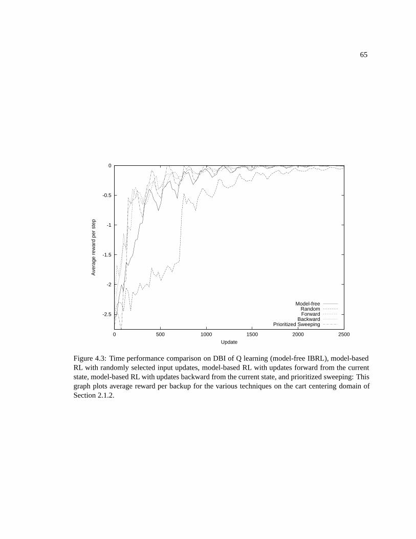
65

-2.5

-2

-1.5

-1

-0.5

0

0 500 1000 1500 2000 2500

Ave

rage

rew

ard

per

step

Update

Model-freeRandomForward

BackwardPrioritized Sweeping

Figure 4.3: Time performance comparison on DBI of Q learning (model-free IBRL), model-basedRL with randomly selected input updates, model-based RL with updates forward from the currentstate, model-based RL with updates backward from the current state, and prioritized sweeping: Thisgraph plots average reward per backup for the various techniques on the cart centering domain ofSection 2.1.2.

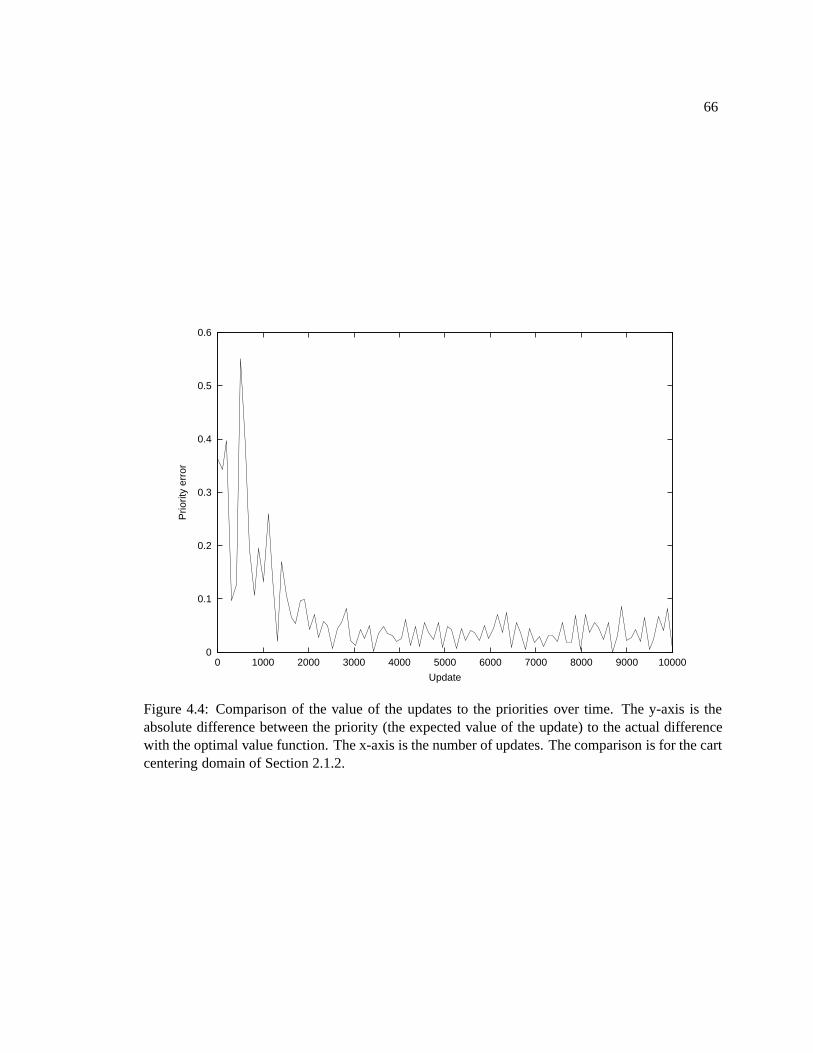
66

0

0.1

0.2

0.3

0.4

0.5

0.6

0 1000 2000 3000 4000 5000 6000 7000 8000 9000 10000

Prio

rity

erro

r

Update

Figure 4.4: Comparison of the value of the updates to the priorities over time. The y-axis is theabsolute difference between the priority (the expected value of the update) to the actual differencewith the optimal value function. The x-axis is the number of updates. The comparison is for the cartcentering domain of Section 2.1.2.

67

agent goes far enough down the wrong path and learns a misleading Q function, it might never

recover. While the algorithm may theoretically converge, the action and state space is large enough

that the near-optimal policies may never be encountered in any reasonable length of time through

basic exploration. The system can be restarted if learning levels off at suboptimal policy. Prior-

itzed sweeping and other model-based algorithms are somewhat more volatile because they take

larger steps based on their estimates. Prioritzed sweeping can use inaccurate value estimates to

converge quickly to a suboptimal and incompetent policy. Nevertheless, prioritized sweeping learns

the fastest of the tested methods and is able to learn policies for more complex tasks.

Much of prioritized sweeping’s increased learning efficiency in comparison to using ran-

dom samples can be attributed simply to its use of the forward and backward samples. Many random

inputs will never occur in normal operation. In fact, the random inputs were intentionally underrep-

resented in the priority queue because their priorities tended to be less reliable and the updates were

of less utility. The prioritized samples are more useful than either straight forward or backward sam-

pling, however. The priorities do aid the search of the agent by broadening the effect of experience.

Repeated updates strictly locally on the current path, i.e. the forward or backward inputs, do not

have the broader effect of sampling with more temporally and spatially distant inputs. Prioritized

sweeping makes the learning process more variable since the updates are more likely to be of greater

magnitude, but sometimes in the wrong direction. Future work will try to better determine how to

better select inputs to update by improving the approximations of the priority calculations.

4.5 Conclusion

I have presented an approach to model-based reinforcement learning in continuous state

spaces. I presented an extension of the prioritized sweeping principle for continuous domains us-

ing instance-based function approximators for the Q function and continuous dynamic Bayesian

networks to represent the model. Our system is able to work with complex conditional density

functions in the DBN utilizing a stochastic sampling method to perform backward inference. In

sum, the method shows promise for problems with continuous states and actions.

68

Chapter 5

Control in Complex Domains

To this point, I have described the learning algorithm for learning basic control tasks. In

this chapter, I detail how the actions can be used together for control in traffic scenarios. While the

instance-based learning algorithm is effective in learning tasks such as lane following and platoon-

ing, more complex tasks, such as route planning and control in traffic, are currently better suited

to hierarchical or otherwise structured control. In traffic, the number of state dimensions increases

greatly as each adjacent vehicle’s state data (relative position and velocity and other information)

is incorporated. Fortunately, the driving environment has a significant amount of structure that can

be used to make the problem tractable. My previous research on driving algorithms yielded an ef-

fective control structure that developed actions through hill climbing[Forbes et al., 1997]. In this

chapter, I show how the performance is improved by using learned actions. Section 5.1 outlines

the methods for control of autonomous vehicles. In order to test our controller algorithms, we have

created a simulator which is detailed in Section 5.2. The results of the evaluations in the simulator

are presented in Section 5.3.

5.1 Hierarchical control

In the Bayesian Automated Taxi project, we develop controllers for autonomous vehicles

in normal highway traffic using a hierarchical decision making architecture [Forbes et al., 1997].

At the highest level, there is a component responsible for overall trip planning and parameters such

as desired cruising speed, lane selection, and target highways. Given these parameters, a driving

module must actually control the vehicle in traffic according to these goals. This task is where I

have concentrated my efforts thus far in the BAT project. The driving module itself can be split up

69

further where it may call upon actions such as lane following or lane changing. Some interaction

between levels will exist. For example, an action such as a lane change must be monitored and in

some cases aborted. I decompose the problem wherever possible while keeping in mind that there

will always be potential interactions between different tasks.

The control has major modes for the driving state such as changing lanes or exiting the

highway. The reason for these modes is that they override the basic driving behavior. For example,

if a controller starts changing lanes, it should continue changing lanes until it has reached the next

lane unless there is some threat. After initiating a lane change to the left, it is not advisable to change

lanes to the right because the previously occupied lane appears to be faster now. Furthermore, when

changing lanes, the vehicle may have some acceleration trajectory to get into a gap between two

cars in the adjacent lane. These modes form the top level of the decision tree, and they dispatch

control to the different modules.

Some of the driving modes are described below:

Basic Maintains lane and target speed while passing vehicles where necessary. An example of the

basic driving structure is given in Figure 5.1.

Continue Lane Change The controller tries to predetermine hazards before changing as much as

possible in making a lane change. In determining whether a lane change is possible, a accel-

eration trajectory is also computed.

Move to Target This mode occurs when the trying to exit or enter a highway. The controller may

need to slow down or speed up to move into a gap in traffic before the junction.

The behavior of the vehicles is governed by target lane and target speed. The target speed

is set upon initialization of the vehicle. The target lane is set depending on the location of its

destination highway. Each vehicle has access to a map object which gives the possible routes from

highway A to highway B. Below, I have given an example of how to act depending on the distance

to the junction.

In general the implementation of the longitudinal control was independent of that of the

lateral control. For more complicated maneuvers such as swerving to avoid an obstacle, this as-

sumption would no longer hold.

The controllers are able to specify high level actions such as lane following instead of the

actual steering control decisions, for example. However, the low level control is still an important

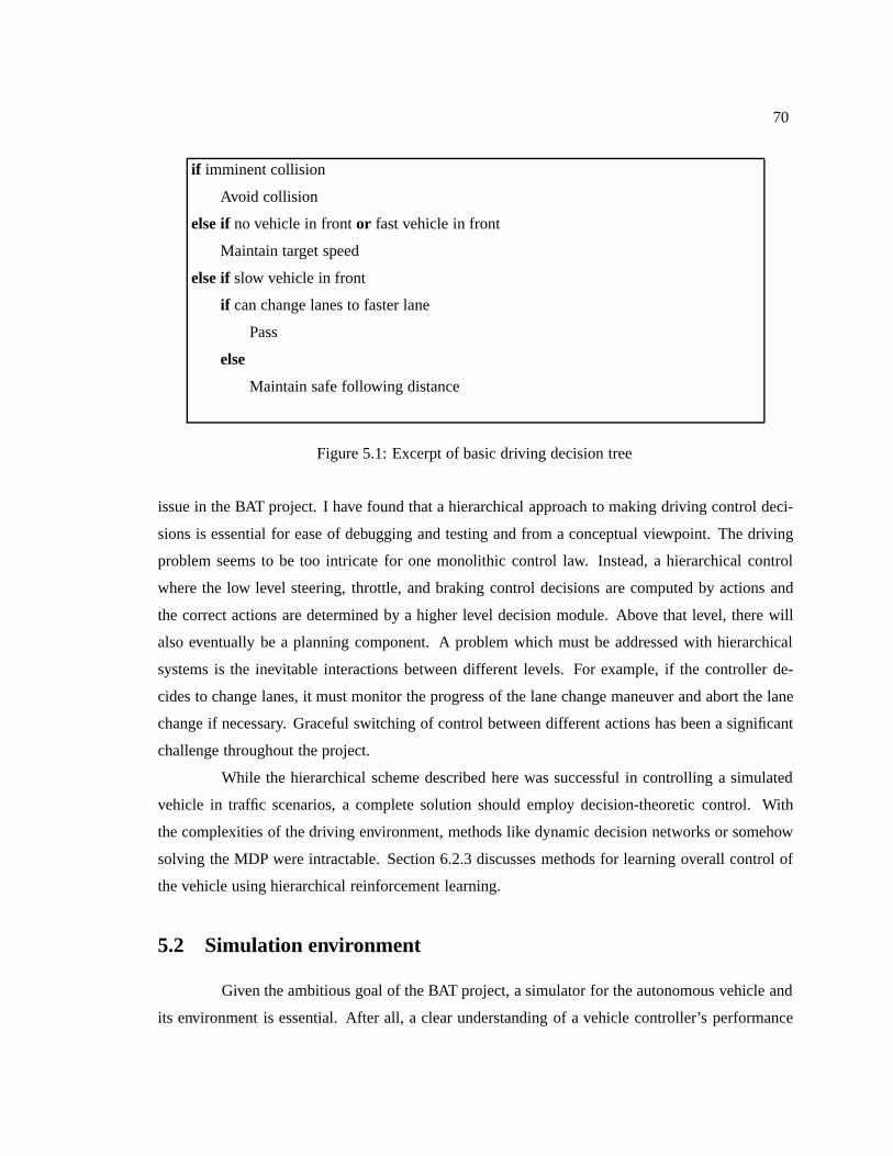
70

if imminent collision

Avoid collision

else if no vehicle in front or fast vehicle in front

Maintain target speed

else if slow vehicle in front

if can change lanes to faster lane

Pass

else

Maintain safe following distance

Figure 5.1: Excerpt of basic driving decision tree

issue in the BAT project. I have found that a hierarchical approach to making driving control deci-

sions is essential for ease of debugging and testing and from a conceptual viewpoint. The driving

problem seems to be too intricate for one monolithic control law. Instead, a hierarchical control

where the low level steering, throttle, and braking control decisions are computed by actions and

the correct actions are determined by a higher level decision module. Above that level, there will

also eventually be a planning component. A problem which must be addressed with hierarchical

systems is the inevitable interactions between different levels. For example, if the controller de-

cides to change lanes, it must monitor the progress of the lane change maneuver and abort the lane

change if necessary. Graceful switching of control between different actions has been a significant

challenge throughout the project.

While the hierarchical scheme described here was successful in controlling a simulated

vehicle in traffic scenarios, a complete solution should employ decision-theoretic control. With

the complexities of the driving environment, methods like dynamic decision networks or somehow

solving the MDP were intractable. Section 6.2.3 discusses methods for learning overall control of

the vehicle using hierarchical reinforcement learning.

5.2 Simulation environment

Given the ambitious goal of the BAT project, a simulator for the autonomous vehicle and

its environment is essential. After all, a clear understanding of a vehicle controller’s performance

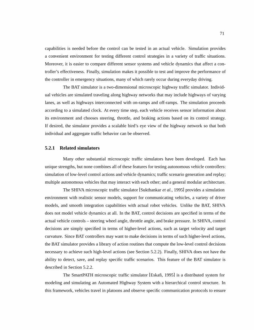
71

capabilities is needed before the control can be tested in an actual vehicle. Simulation provides

a convenient environment for testing different control strategies in a variety of traffic situations.

Moreover, it is easier to compare different sensor systems and vehicle dynamics that affect a con-

troller’s effectiveness. Finally, simulation makes it possible to test and improve the performance of

the controller in emergency situations, many of which rarely occur during everyday driving.

The BAT simulator is a two-dimensional microscopic highway traffic simulator. Individ-

ual vehicles are simulated traveling along highway networks that may include highways of varying

lanes, as well as highways interconnected with on-ramps and off-ramps. The simulation proceeds

according to a simulated clock. At every time step, each vehicle receives sensor information about

its environment and chooses steering, throttle, and braking actions based on its control strategy.

If desired, the simulator provides a scalable bird’s eye view of the highway network so that both

individual and aggregate traffic behavior can be observed.

5.2.1 Related simulators

Many other substantial microscopic traffic simulators have been developed. Each has

unique strengths, but none combines all of these features for testing autonomous vehicle controllers:

simulation of low-level control actions and vehicle dynamics; traffic scenario generation and replay;

multiple autonomous vehicles that may interact with each other; and a general modular architecture.

The SHIVA microscopic traffic simulator [Sukthankar et al., 1995] provides a simulation

environment with realistic sensor models, support for communicating vehicles, a variety of driver

models, and smooth integration capabilities with actual robot vehicles. Unlike the BAT, SHIVA

does not model vehicle dynamics at all. In the BAT, control decisions are specified in terms of the

actual vehicle controls – steering wheel angle, throttle angle, and brake pressure. In SHIVA, control

decisions are simply specified in terms of higher-level actions, such as target velocity and target

curvature. Since BAT controllers may want to make decisions in terms of such higher-level actions,

the BAT simulator provides a library of action routines that compute the low-level control decisions

necessary to achieve such high-level actions (see Section 5.2.2). Finally, SHIVA does not have the

ability to detect, save, and replay specific traffic scenarios. This feature of the BAT simulator is

described in Section 5.2.2.

The SmartPATH microscopic traffic simulator [Eskafi, 1995] is a distributed system for

modeling and simulating an Automated Highway System with a hierarchical control structure. In

this framework, vehicles travel in platoons and observe specific communication protocols to ensure

72

that basic maneuvers are performed safely and efficiently. SmartPATH also provides an elaborate

3-D display of the simulation, with the ability to view the traffic from any vantage point, including

from the driving position of any vehicle. Because SmartPATH was developed primarily for research

using the AHS paradigm, which features centralized control, individual vehicles aren’t provided

the level of autonomy necessary for testing individual vehicle controllers. For example, a vehicle

in SmartPATH could request a lane change but would need the central controller’s permission to

execute it.

The PHAROS microscopic traffic simulator [Reece, 1992] models urban traffic environ-

ments. It provides for the explicit representation of traffic control devices, such as lines, road mark-

ing, signs, and traffic signals. Unlike the BAT simulator, PHAROS can model only one autonomous

vehicle at a time. All other vehicles follow a “zombie” control strategy, which operates by follow-

ing a preselected set of actions rather than making decisions based on sensor information. Further-

more, PHAROS simulates vehicle lane information at an abstract level. This means that vehicles in

PHAROS cannot abandon this abstraction to make ad hoc decisions, for example, to drive around a

stalled car.

5.2.2 Design of the simulator

In developing the BAT simulator, we have tried to make it as flexible and extensible as

possible. At the same time, the design reflects a focus on developing controllers for autonomous

vehicles that operate in unrestricted traffic. Given this emphasis, we developed the following re-

quirements:

� In general, traffic scenarios for testing controllers should resemble real-world traffic patterns.

This means that the user should be able to specify a highway topology as well as probability

distributions for generating traffic. It also means that the traffic should consist of various types

of vehicles, each with parameterizable behaviors.

� Since there are many kinds of cars and since they operate in a wide range of physical condi-

tions, e.g., clear vs. rainy weather, the simulation should allow controllers to be tested with

different vehicle dynamics and models of the physical environment.

� The simulation should allow sensor models with varying levels of detail. These can be models

of real-world sensors or of abstract sensors. For example, a simple, noisy radar sensor could

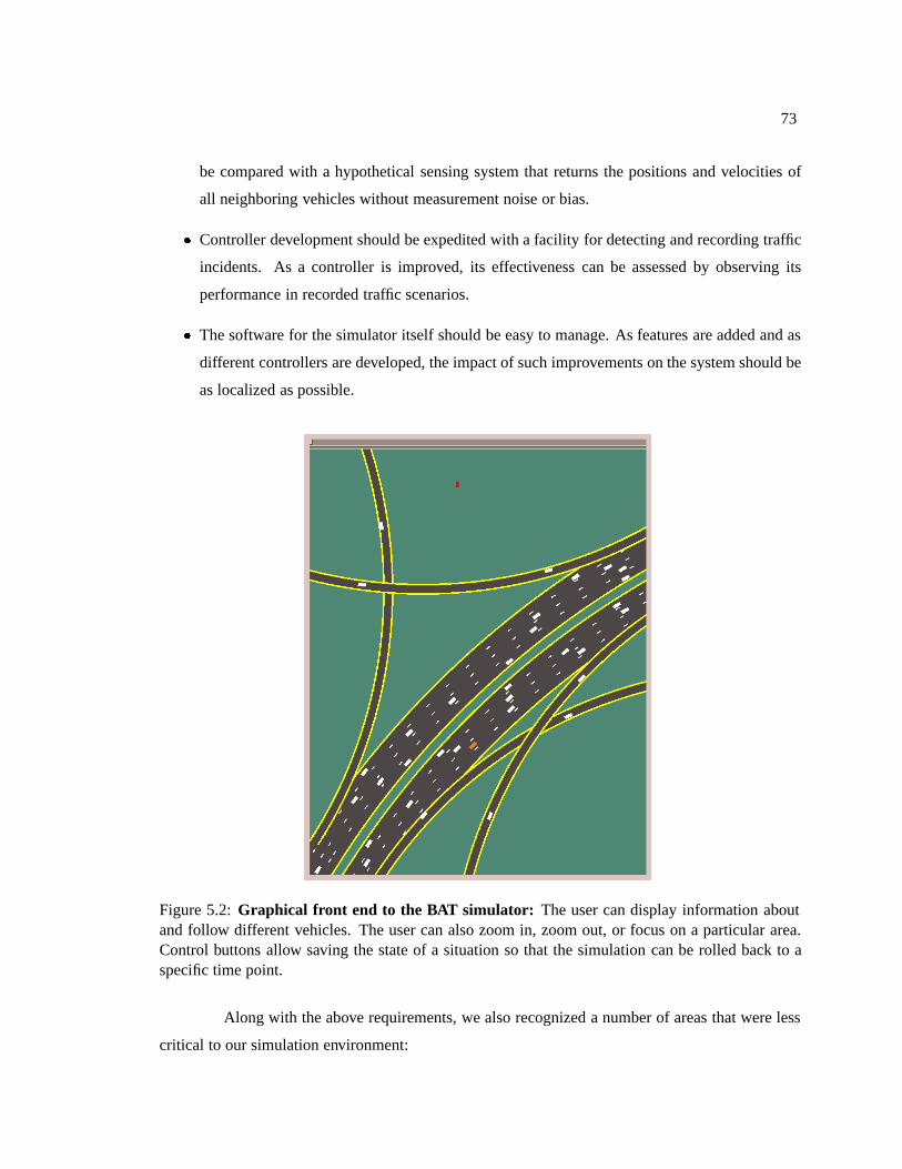
73

be compared with a hypothetical sensing system that returns the positions and velocities of

all neighboring vehicles without measurement noise or bias.

� Controller development should be expedited with a facility for detecting and recording traffic

incidents. As a controller is improved, its effectiveness can be assessed by observing its

performance in recorded traffic scenarios.

� The software for the simulator itself should be easy to manage. As features are added and as

different controllers are developed, the impact of such improvements on the system should be

as localized as possible.

Figure 5.2: Graphical front end to the BAT simulator: The user can display information aboutand follow different vehicles. The user can also zoom in, zoom out, or focus on a particular area.Control buttons allow saving the state of a situation so that the simulation can be rolled back to aspecific time point.

Along with the above requirements, we also recognized a number of areas that were less

critical to our simulation environment:

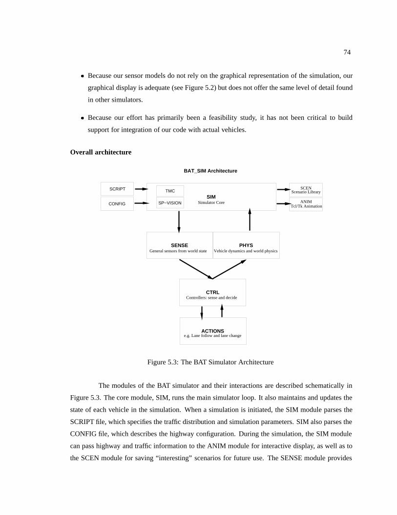
74

� Because our sensor models do not rely on the graphical representation of the simulation, our

graphical display is adequate (see Figure 5.2) but does not offer the same level of detail found

in other simulators.

� Because our effort has primarily been a feasibility study, it has not been critical to build

support for integration of our code with actual vehicles.

Overall architecture

BAT_SIM Architecture

SCRIPT

CONFIG

SIMSimulator Core

CTRL

ACTIONS

SENSEGeneral sensors from world state

PHYSVehicle dynamics and world physics

Controllers: sense and decide

e.g. Lane follow and lane change

SCENScenario Library

ANIMTcl/Tk Animation

TMC

SP−VISION

Figure 5.3: The BAT Simulator Architecture

The modules of the BAT simulator and their interactions are described schematically in

Figure 5.3. The core module, SIM, runs the main simulator loop. It also maintains and updates the

state of each vehicle in the simulation. When a simulation is initiated, the SIM module parses the

SCRIPT file, which specifies the traffic distribution and simulation parameters. SIM also parses the

CONFIG file, which describes the highway configuration. During the simulation, the SIM module

can pass highway and traffic information to the ANIM module for interactive display, as well as to

the SCEN module for saving “interesting” scenarios for future use. The SENSE module provides

75

the controllers with percepts based on the world state maintained by the simulator. The PHYS

module takes as input a controller output in the form of a steering, throttle, and braking decision.

The controller can also use routines in the ACTIONS module to determine, for example, what

steering angle will allow the vehicle to follow its lane using a particular control law. Finally, the

COMM module can perform network socket communication with other processes, including the

SmartPATH animator, and the MISC module provides utility functions for use by any of the other

modules. The figure also includes two applications built on top of the simulator: a TMC (Traffic

Management Center) and SP VISION, an extension that uses the SmartPATH animator to simulate

a stereo vision system.

Sensor and physics models

The sensing and physics modules provide a layer of abstraction between the controllers

and the world state as maintained by the simulator. The sensing routines provide the controllers

with a consistent representation of the world state in the simulation. The information generally

consists of information about the car itself and the cars which are within its sensor range. There

are a number of different types of sensing and levels of detail. For example, the simple though not

realistic sensor model may provide simulator information directly to a vehicle controller. A more

sophisticated model may simulate noise, specific kinds of sensors, limited sensor range, and may

infer additional information about neighboring cars.

The physics routines maintain and update the kinematic state of the vehicles based on

the control decisions of the controller. The controllers pass their steering, throttle, and braking

decisions to the physics module. The physics module also handles all other interactions of the

controller with the environment. There are a number of different levels of physics which correspond

to different models of dynamics. The most complicated model that we use is for a front-wheel drive

automobile using 18 state variables. These variables describe the dynamics of the chassis, engine,

tire, suspension, and steering, throttle, and brake actuators. (The hypothetical vehicle from which

the parameters are taken is a Lincoln Town Car engine with a Toyota Celica chassis, although other

vehicle-specific parameters could be used as well. This model of vehicle dynamics provides an

accurate representation of the physical plant of an automobile [Tomizuka et al., 1995; Hedrick et

al., 1993; Peng, 1992].)

76

Lower-level library of action routines

The actions module provides a library of routines for calculating lower level control de-

cisions. These routines provide a controller-independent application of a control law based on

a particular vehicle state. Developing new controllers is thus much easier because the program-

mer can simply plug-in already developed low-level control decisions and concentrate on choosing

higher-level actions. Some of the actions are continuously parameterizable. For example, tracking

the vehicle in front at distance % meters which will return a throttle decision that keeps the car %

meters from the vehicle in front. Other actions, such as changing lanes, are discrete.

To create the action routines, we generally used a proportional plus derivative controller

where:

Æ�7!��!��

and where 7!��!� is a low-level control decision. The error is denoted by �, which may, for example,

be the distance from the center of the lane to be followed during lane following. The parameters

� and �� are constants which I determined using a technique called hill-climbing search. In

this method, � and �� are set to arbitrary initial values and are iteratively improved, based on

how they affect a controller’s performance in a training scenario. For example, poor performance

in lane following results from diverging from the lane, excessive lateral acceleration, and off-road

excursions.

Scripting and configuration

In order to fully test the control algorithms, the simulation must include realistic and

challenging traffic patterns and highway topologies. The simulation scripts handle the creation of

the traffic. A script contains a list of car generation commands, each of which describes distributions

for vehicle type (including controller, size, and color), the time a vehicle enters the freeway, and the

goals of a vehicle. A script also contains commands to control various simulation parameters.

These may involve something as comprehensive as the length of the simulation or as particular as

the variance on minimum following distance for a specific kind of controller.

Highway networks in the BAT simulator are described as a set of highways connected by

junctions. A highway is defined as an uninterrupted stretch of road with a constant number of lanes.

The highways themselves are constructed from straight and circular arc segments. The junctions

provide a way to add on-ramps, off-ramps, changes in the number of lanes, splits, merges and most

other highway formations. The highway configuration files are compatible with SmartPATH version

77

2.0 (without the extensions for AHS, such as automated versus manual lanes). The SmartPATH

User’s Manual gives details on the configuration files[Eskafi and Khorramabadi, 1994].

Scenario generation

Scenario generation and incident detection facilitate the development and testing of con-

trollers. The simulation can be instrumented so that when a particular “incident” occurs, the state of

the simulator is rolled back a specified amount of time and saved. By “incident,” I mean any sort of

interesting traffic event, which may include crashes or just dips in the performance of a particular

vehicle. A user can also roll back time and save the state manually while viewing the simulation in

progress. In order to roll back the state of the simulation, the simulator and the individual controllers

must periodically save their state. These saved states together constitute a traffic scenario. Once a

scenario has been saved, the user may choose to vary some parameters or make other changes and

then restart the simulator from that point.

A scenario can be saved for future testing to a scenario library. I am currently working

towards creating a large scenario library to verify and measure the performance of a controller on a

number of difficult situations.

5.2.3 Controllers

Given the design of the modules in the simulator, a controller needs to have four major

routines:

Initializer: Called upon creation of the car. Initializes and returns the controller data structure.

Controller: Called every time step. Senses the environment from a sensor module and outputs its

decision to one of the physics modules.

Recorder: Called at some specified interval. Records data needed for rollback of the system.

Restarter: Called up restart of a scenario. Sets the controller state to the recorded state.

There are a number of different controllers in the system. These include: a vehicle which

stalls, simple lane followers, the Bayesian Automated Taxi itself, and “smart” drones. The parame-

terized stochastic smart drones have perfect sensing and can provide a number of interesting traffic

patterns. The drones try to achieve a particular (possibly varying) target speed while driving to-

ward their destination. In order to reach its destination, a drone sets a target lane on each highway.

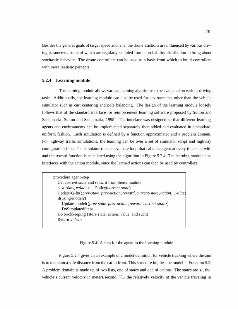
78

Besides the general goals of target speed and lane, the drone’s actions are influenced by various driv-

ing parameters, some of which are regularly sampled from a probability distribution to bring about

stochastic behavior. The drone controllers can be used as a basis from which to build controllers

with more realistic percepts.

5.2.4 Learning module

The learning module allows various learning algorithms to be evaluated on various driving

tasks. Additionally, the learning module can also be used for environments other than the vehicle

simulator such as cart centering and pole balancing. The design of the learning module loosely

follows that of the standard interface for reinforcement learning software proposed by Sutton and

Santamaria [Sutton and Santamaria, 1998]. The interface was designed so that different learning

agents and environments can be implemented separately then added and evaluated in a standard,

uniform fashion. Each simulation is defined by a function approximator and a problem domain.

For highway traffic simulations, the learning can be over a set of simulator script and highway

configuration files. The simulator runs an evaluate loop that calls the agent at every time step with

and the reward function is calculated using the algorithm in Figure 5.2.4. The learning module also

interfaces with the action module, since the learned actions can then be used by controllers.

procedure agent-stepGet current-state and reward from Sense module � �� Policy(current-state)Update-Q-fn(�prev-state� prev-action� reward� current-state� action� � value)if(using-model?)

Update-model(�prev-state� prev-action� reward� current-state�)DoSimulatedSteps

Do bookkeeping (store state, action, value, and such)Return � ��

Figure 5.4: A step for the agent in the learning module

Figure 5.2.4 gives an an example of a model definition for vehicle tracking where the aim

is to maintain a safe distance from the car in front. This structure implies the model in Equation 5.2.

A problem domain is made up of two lists, one of states and one of actions. The states are ��, the

vehicle’s current velocity in meters/second, �� , the relatively velocity of the vehicle traveling in

79

make-problem-domain "VEHICLE_TRACK" {{

{"Va" 0.0 45.0 {"Va" "accel"} {}}{"Vab" 0.0 45.0 {"Vab" "accel"} {}}{"Dab" 0.0 150.0 {"Dab" "Vab"} {}}{"REWARD" -1000 0.0 {"iw*Dab"}

{{"Dab" "Dab"} {"accel" "accel"}}}{"iw*Dab" 0 1.0 {} {}}

}{ {"accel" -5.0 3.0} }

}

Figure 5.5: An example of a problem domain declaration for vehicle tracking. The problem domaindeclaration defines the model structure.

front, -�+, the distance to the vehicle in front. Associated with the state is �, the current reward,

and �� . �� is a function that defines its argument is “in the world” or within

some bounds. In this case, �� determines whether the car in front’s distance is either

too small (a crash) or too far (lost track). Besides, “in the world,” there are other functions which

can be used on the input to create the model such as sine and cosine. Each state has associated with

it the inputs that it depends on as well as any combinations of inputs of which it is a combination.

The learning module is extensible in that any number of of parametric and instance-based function

approximators can be implemented and added, as well as domain model learning algorithms and

utility routines such as function optimizations for policy computation.

5.2.5 Implementation and results

The simulator itself is written in C, and the graphical user interface is implemented in

Tcl/Tk. To enhance the modularity of the system while maintaining compatibility with existing

code, I created a framework that facilitates a more object-oriented structure of the system. The

system has been successfully ported to a variety of systems including HP-UX, Linux on i386 and

PPC architectures, Solaris, and Mac OS X. The simulator is currently going through a major revision

and will be implemented in C++ as part of the never ending effort to make the system stable in the

presence of constant changes. At some point, I would like to release the simulator for public use.

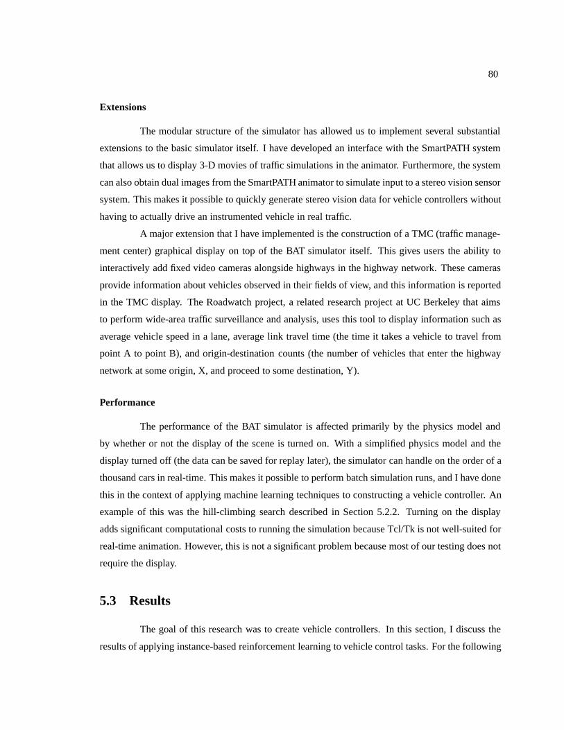
80

Extensions

The modular structure of the simulator has allowed us to implement several substantial

extensions to the basic simulator itself. I have developed an interface with the SmartPATH system

that allows us to display 3-D movies of traffic simulations in the animator. Furthermore, the system

can also obtain dual images from the SmartPATH animator to simulate input to a stereo vision sensor

system. This makes it possible to quickly generate stereo vision data for vehicle controllers without

having to actually drive an instrumented vehicle in real traffic.

A major extension that I have implemented is the construction of a TMC (traffic manage-

ment center) graphical display on top of the BAT simulator itself. This gives users the ability to

interactively add fixed video cameras alongside highways in the highway network. These cameras

provide information about vehicles observed in their fields of view, and this information is reported

in the TMC display. The Roadwatch project, a related research project at UC Berkeley that aims

to perform wide-area traffic surveillance and analysis, uses this tool to display information such as

average vehicle speed in a lane, average link travel time (the time it takes a vehicle to travel from

point A to point B), and origin-destination counts (the number of vehicles that enter the highway

network at some origin, X, and proceed to some destination, Y).

Performance

The performance of the BAT simulator is affected primarily by the physics model and

by whether or not the display of the scene is turned on. With a simplified physics model and the

display turned off (the data can be saved for replay later), the simulator can handle on the order of a

thousand cars in real-time. This makes it possible to perform batch simulation runs, and I have done

this in the context of applying machine learning techniques to constructing a vehicle controller. An

example of this was the hill-climbing search described in Section 5.2.2. Turning on the display

adds significant computational costs to running the simulation because Tcl/Tk is not well-suited for

real-time animation. However, this is not a significant problem because most of our testing does not

require the display.

5.3 Results

The goal of this research was to create vehicle controllers. In this section, I discuss the

results of applying instance-based reinforcement learning to vehicle control tasks. For the following

81

tasks, the controller controls the accelerator or throttle � and the steering angle . For some models

of vehicle dynamics, there is a separate brake pressure variable, but for the purposes of learning, the

brake pressure is viewed as the complement of the throttle, i.e. brake pressure is negative throttle

angle.

5.3.1 Actions to be learned

In lane following, the object is to have the vehicle control the steering so that the vehicle

follows the center of a predetermined lane as closely as possible without ever driving off the road.

Speed and highway networks are varied. The evaluation highway networks consisted of a figure-

eight track, an oval, and a road with a variety of sharp curves (see Figure 5.6).

Figure 5.6: Two highway networks for training: a figure-eight network and a winding highway witha number of tight curves

The following are the input (state and action) variables:

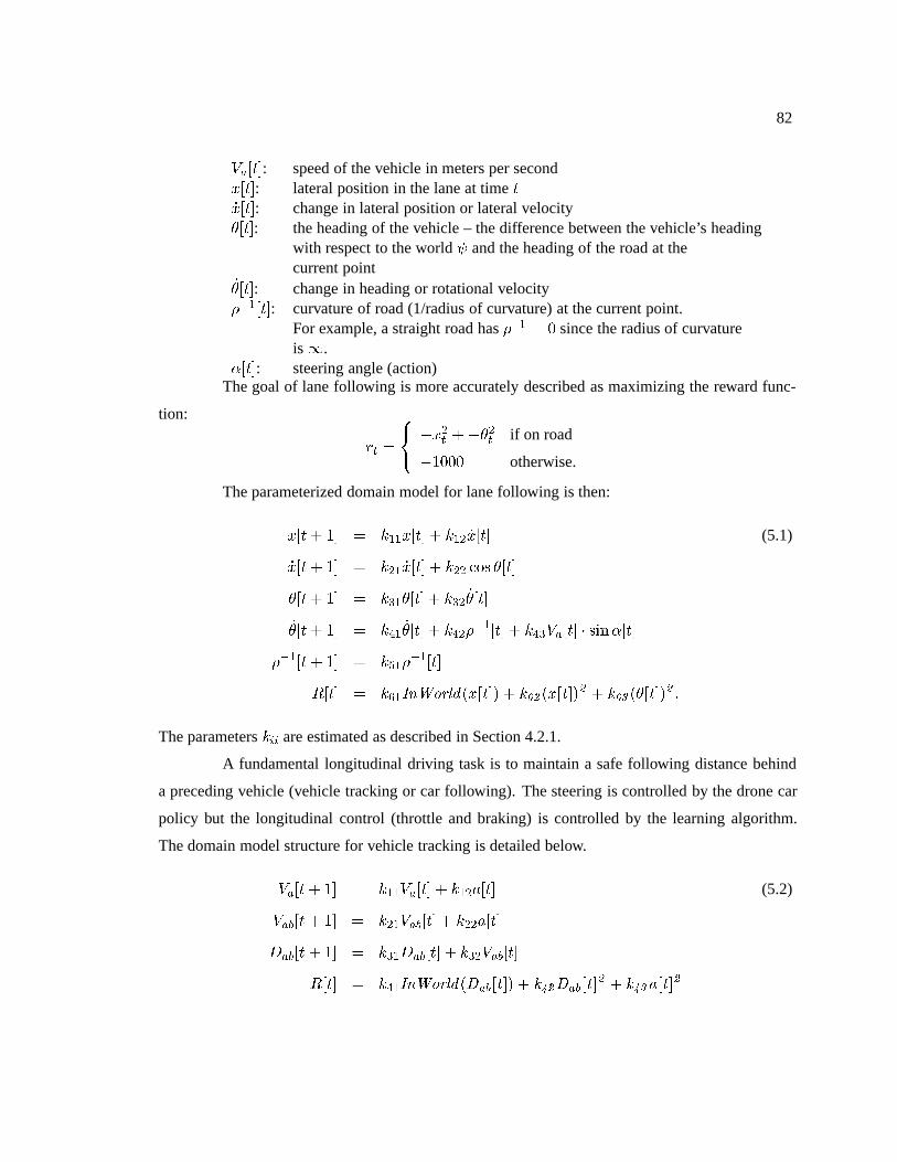
82

��: speed of the vehicle in meters per second.��: lateral position in the lane at time ��.��: change in lateral position or lateral velocity6��: the heading of the vehicle – the difference between the vehicle’s heading

with respect to the world ( and the heading of the road at thecurrent point

�6��: change in heading or rotational velocity&��: curvature of road (1/radius of curvature) at the current point.

For example, a straight road has &�� since the radius of curvatureis �.

��: steering angle (action)The goal of lane following is more accurately described as maximizing the reward func-

tion:

��

�� .�� 6�� if on road

�� otherwise.

The parameterized domain model for lane following is then:

.�� .�� .�� (5.1)

�.�� .�� "�� 6��

6�� 6�� 6��

�6�� 6�� &�� ( ��

&�� &��

�� 6��

� �

The parameters �� are estimated as described in Section 4.2.1.

A fundamental longitudinal driving task is to maintain a safe following distance behind

a preceding vehicle (vehicle tracking or car following). The steering is controlled by the drone car

policy but the longitudinal control (throttle and braking) is controlled by the learning algorithm.

The domain model structure for vehicle tracking is detailed below.

�� (5.2)

��

-� �� -� ��

��

�

83

5.3.2 Simple vehicle dynamics

As stated in Section 5.2.2, the simulator has a number of different vehicle dynamics mod-

els. The vehicle dynamics for the simple idealized case are:

��

�( �� (

1

where 1 is the wheelbase or the length of the vehicle and ( is the change in the vehicle’s heading.

For this model, one can derive near-optimal hand-coded controllers. For a curve with a radius of

curvature &, the correct tire angle � �"��(�1�& and a PD controller can be used to correct

the vehicle within the lane. Maintaining the speed can be done by simply setting � to zero. Tracking

a vehicle is done by using a PD controller where the gains have been fine tuned by hill climbing.

The results for lane following with simple dynamics are in Figure 5.7. Model-free IBRL

and prioritized sweeping are compared to a derived controller for lane following. The speeds were

varied between 15 and 35 ��. Neither of the learned controllers exceeded the performance of the

analytically-derived control, but they did both come rather close. Both the model-free and model-

based methods were able to successfully navigate all of the tracks at all of the various speeds.

Similarly, the controllers were applied to the vehicle tracking problem for simple dynam-

ics in Figure 5.8. The goal was to stay at ideal following distance which is determined by the

simulator based on the velocity of the lead vehicle, the velocity and acceleration of the following

vehicle, and the acceleration and jerk capabilities of the lead and following vehicle. The goal is to

maintain the ideal following distance error �� . The lead vehicle varied its speeds between 5

and 35 ��. The reward function was:

��

��

�� if on road

�� if out of range

�� if crashed.

5.3.3 Complex vehicle dynamics

A more realistic set of vehicle dynamics is the combined lateral and longitudinal model

developed by PATH researchers [Tomizuka et al., 1995; Hedrick et al., 1993]. As mentioned in

Section 5.2.2, it models the longitudinal dynamics of a Lincoln Town Car and the lateral dynamics

of a Toyota Celica. This model is among the most accurate vehicle models available, although even

84

-1200

-1000

-800

-600

-400

-200

0

0 200 400 600 800 1000 1200 1400 1600 1800 2000

Acc

rew

ard

per

tria

l

Trial

Hand codedModel-free

Prioritized sweeping

Figure 5.7: Lane following (Q, PS, Control-theoretic): This figure shows the results for lane follow-ing with simple vehicle dynamics. The analytically-derived hand-coded controller performance is-0.72 reward/trial, while the prioritized sweeping and model-free controllers reached -2 and -8 re-spectively after 2500 trials. The learning controller only controls the steering angle. Each controllerwas run on three highway networks for a maximum of 200 seconds.

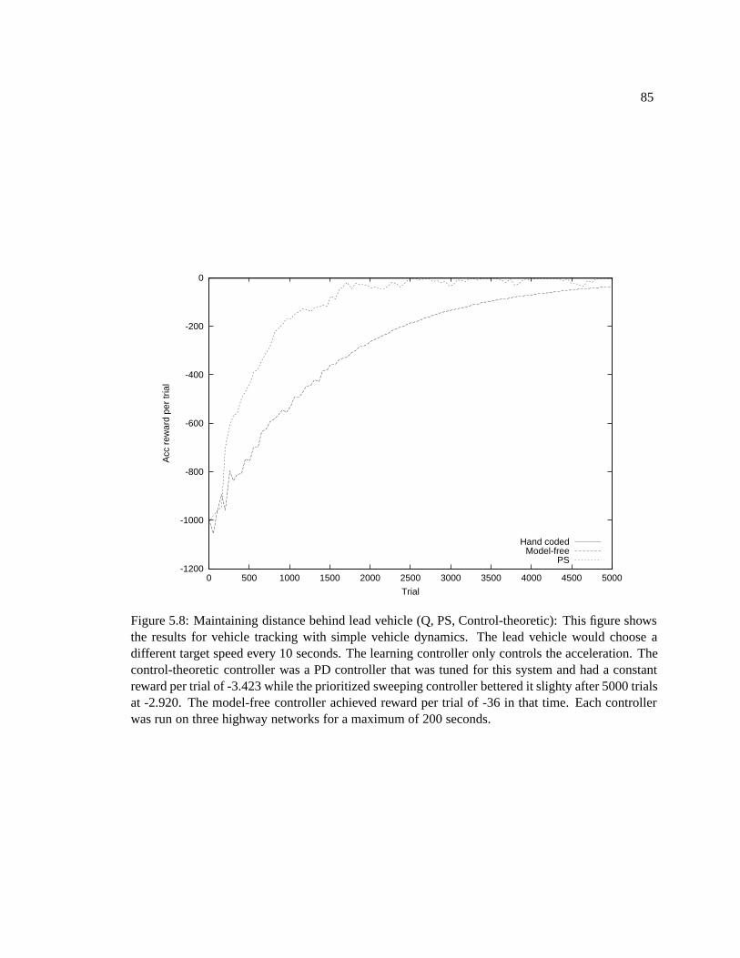
85

-1200

-1000

-800

-600

-400

-200

0

0 500 1000 1500 2000 2500 3000 3500 4000 4500 5000

Acc

rew

ard

per

tria

l

Trial

Hand codedModel-free

PS

Figure 5.8: Maintaining distance behind lead vehicle (Q, PS, Control-theoretic): This figure showsthe results for vehicle tracking with simple vehicle dynamics. The lead vehicle would choose adifferent target speed every 10 seconds. The learning controller only controls the acceleration. Thecontrol-theoretic controller was a PD controller that was tuned for this system and had a constantreward per trial of -3.423 while the prioritized sweeping controller bettered it slighty after 5000 trialsat -2.920. The model-free controller achieved reward per trial of -36 in that time. Each controllerwas run on three highway networks for a maximum of 200 seconds.

86

this incredibly detailed system does not perfectly represent the complexity of a real vehicle. For

example, the model assumes that there is no slip at the wheels and that there are no time delays

in combustion dynamics. Nevertheless, the system is decidedly difficult to control. As shown in

Table 5.1 and Table 5.2, the learned actions do significantly outperform a painstakingly developed

hand-coded policy. Moreover, the learned controllers were able to achieve greater functionality.

On the test track with curves, the hand-coded controller was not able to navigate the entire route

at �� without driving off the road. The learned controller was able to make it through the

entire track. Longitudinal control, in particular, is much more challenging when using the complex

dynamics. Just maintaining the current speed can be difficult, since the road, aerodynamic, and

engine forces act against the vehicle and having no throttle will result in the vehicle slowing down.

The same structure was used for models as in the simple dynamics. In the case of the complex

dynamics, it was not possible to learn the model exactly since it no longer exactly fit the true system,

but using the mean of the various state variables from the model was still quite effective.

Algorithm Reward/Trial Trials required

Hand-coded -126.44 n/aPrioritized Sweeping -9.24 21k

Table 5.1: Lane following performance with complex vehicle dynamics (PS, Hand-coded). Thehand-coded controller always failed at high speeds on the curves highway.


Hand-coded PD control -11.84 n/aPrioritized Sweeping -6.64 11.7k

Table 5.2: Steady-state speed tracking performance with complex vehicle dynamics (PS, Hand-coded)

Another benefit of using a model-based method is that a model, once learned, can be

used for many different tasks. Lane following and lane changing have the same model, but the task

is slightly different. In lane following the goal is to navigate towards the center of the lane. In

lane changing, the goal just shifts from the center of the current lane to that of an adjacent lane.

The evolution of the state variables such as lateral position, heading, and so on remain the same.

In learning, one can use an already primed model to speed up the overall learning process. For

87

example, using a primed model from the lane following experiment of Table 5.1, the prioritized

sweeping showed a modest improvement in learning efficiency (about 120 trials faster).

5.3.4 Platooning

A problem of interest is how to control the lead vehicle of a platoon[Godbole and Lygeros,

1993]. The goal is to maintain a prescribed inter-platoon distance behind the preceding vehicle and

match its speed as closely as possible. More precisely, a controller must minimize the following

quantities:

�� .�� .��

�.�

�� .�� .� � 0�� >� �.� � >�

where �� is the relative velocity of the platoon in front expressed as a percentage of the velocity of

the ��! platoon. �� is the error between the actual and safe inter-platoon distance. Steady state is

where �� and �� .

Godbole and Lygeros developed a controller that uses different control laws in different

regions of the state space. Simulation and experimentation suggested that a single control law would

not give acceptable performance. The � � � plane is separated into four regions based on careful

study of the traffic behavior on an automated freeway. Global control is performed by a weighted

average of 4 control laws. Table 5.3 shows the comparison of the learned controller to the platooning

controller given the following reward function:

��

� � ��

��

where � is the acceleration, �� is the jerk and �� are normalizing factors. The two controllers per-

formed similarly under observation. The explicit platooning controller was more precise in main-

taining following distance. However, the learned controller did a better job in the panic stop and

start situations. It is reasonable to assume that the Godbole and Lygeros controller could be be

changed to better handle that case, but the point is that the reinforcement learning controller could

learn a competent policy and adapt to the task as specified by the reward function.

5.3.5 Driving scenarios

I used the learned policies of Chapter 4 in the place of the hand-coded methods that the

controllers normally used. Using prioritized sweeping to learn the lane change, lane follow, maintain

88


Godbole & Lygeros -123.97 n/aPrioritized Sweeping -117.24 13k

Table 5.3: Platooning (PS vs. Platoon control): In each trial (250 seconds) on an oval track, thepreceding vehicle would pick a random target speed every 15 seconds. Once a simulation, the carwould slow down to �� at a rapid rate (��) to simulate panic braking.

speed, and track front vehicle actions individually, the driving decision tree used the learned actions

in place of the hand coded versions. In training the actions, they were tested at the same speeds as

they would be tested as part of the overall controller. While the individual actions were learned in

the absence of traffic, the actions were effective when used in traffic since they had been tested in a

wide variety of speeds and were generally more precise than the hand-coded controllers.

Controllers were tested on a variety of scenarios including:

� Free flowing traffic on a straight road

� Using the 2 loop track in Figure 5.6, there were three staggered slow (��) vehicles which

blocked three of the four lanes. This formed a general traffic congestion in the loop as the

simulation continued to create cars in each lane at a rate of 2000 new vehicles per lane per

hour. The controller had target of reaching the “fast” lane and continuing at its target speed

(��).

� Using the simulated bay area highway network in Figure 5.9, the vehicle had to cross the

highway through steady traffic (between 1000 and 2000 vehicles created per lane per hour) to

its target highway.

The maximum length of each scenario ranged in length from 30 seconds to 300 seconds. The

third scenario caused the most trouble because it was very difficult to find the gaps in the traffic to

change into and then change with proper acceleration trajectory. Also, the other vehicles had their

own goals, so the vehicle had to avoid them. None of the controllers modeled the state of the other

vehicles, so they would not, for example, anticipate other vehicles changing lanes. The performance

of the controllers measured by the above reward function is shown in Table 5.4. Using the learned

actions with the same decision tree controller worked better in most cases. Primarily, the learned

actions were more robust (being more effective at a broad range of speeds), so that there was more

89

Actions Crashes per 1000s

Hand coded & tuned 1.18Prioritized Sweeping 0.97

Table 5.4: Accident rate in difficult scenarios: Running over a set of scenarios described above ofvarying traffic densities. In normal traffic, this rate decreases by several orders of magnitude.

room for error in making high-level decisions. As an example, rate of successful completion of lane

changes increased from 97.4% to 99.2% in the scenarios.

5.4 Conclusions

The reinforcement learning methods developed in this dissertation are effective for vehicle

control problems. I devised a hierarchical control scheme that handles most freeway driving tasks.

By splitting up driving into lateral and longitudinal actions such as lane following and maintaining

speed respectively, driving becomes more tractable. Using a hierarchical structure is also useful for

learning and developing modular controllers. These controllers are tested in the BAT project simu-

lator. Controllers are iteratively improved by running on a set of scenarios, evaluating, modifying

the controller, and then rerunning. Similarly, actions can be learned automatically using reinforce-

ment learning techniques. The instance-based reinforcement learning methods were evaluated on

lane following, vehicle following, and other tasks. Prioritized sweeping using the instance-based Q

function approximation technique was particularly effective in learning control for vehicle control

tasks and shows promise for other dynamical control tasks.

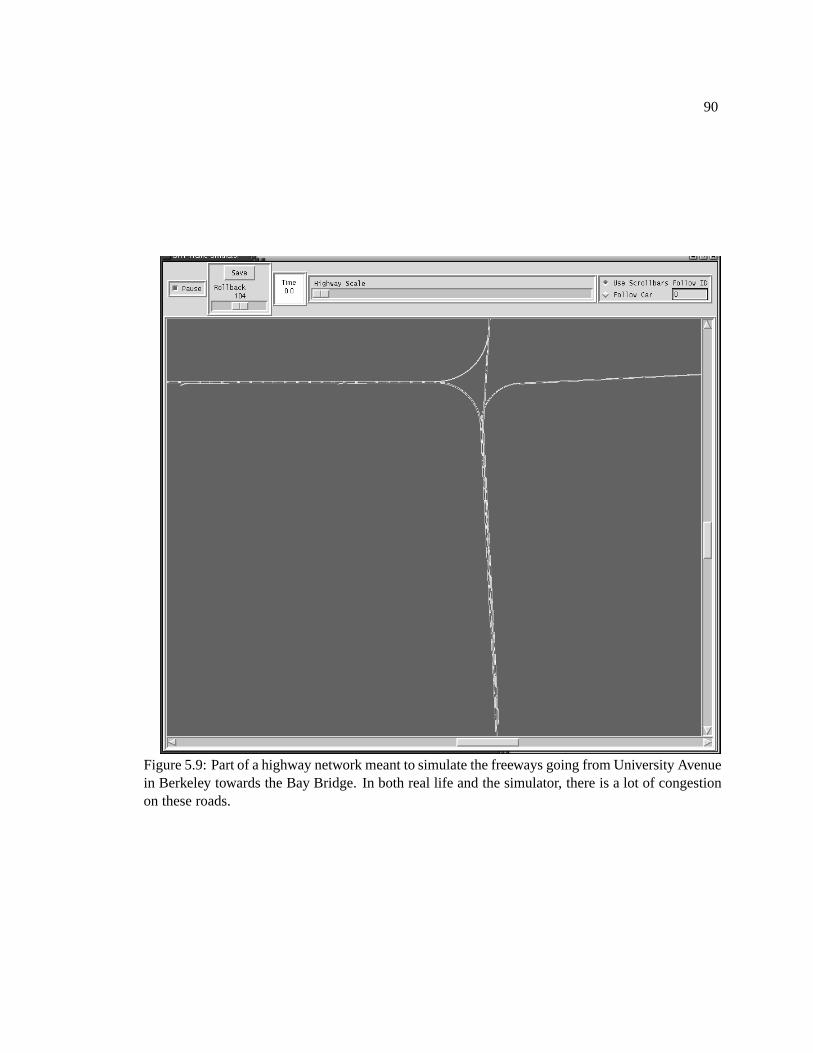
90

Figure 5.9: Part of a highway network meant to simulate the freeways going from University Avenuein Berkeley towards the Bay Bridge. In both real life and the simulator, there is a lot of congestionon these roads.

91

Chapter 6

Conclusions and Future Work

This chapter summarizes the contributions of this dissertation and suggests future direc-

tions for research.

The problem of creating a system to control autonomous vehicles has obvious and helpful

applications. Road congestion and safety issues are not going away. We have, obviously, a long

way to go, but this dissertation is a small step on the road to the eventual creation of BATs. It has

focused on one portion of the problem: learning the subtasks of autonomous vehicle control from

experience. Specifically, I have broken down the experience of driving into certain components,

such as maintaining lane position and regulating the distance behind another car. In order to achieve

these tasks, I developed an algorithm called instance-space based reinforcement learning, a method

in which past experiences are stored, maintained and then generalized.

6.1 Summary of contributions

The first contribution of the dissertation is a method for estimating and maintaining the

value of actions in states by storing instances of previous experiences. Instance-based reinforcement

learning proved effective in learning control policy for various tasks, even when there was no prior

information about the task. Vehicles were able to perform lane following and car following when

faced with a completely new environment. Furthermore, they were able to maintain the estimate of

value in the presence of input of new examples with changing task distributions and catastrophic

interference.

Additionally, I created an algorithm for model-based reinforcement learning for contin-

uous state and action spaces. This algorithm uses state transition examples to build a structured

92

state transition and reward model. It uses experience to adjust the estimated value of states, and

then uses that model and the utility function to update the policy. Within this framework, the agent

is able to exploit the structure in the environment and learn in more complex domains. Efficient

learning is accomplished using a model-based algorithm called prioritized sweeping that focuses

extra planning in the areas of the state-action space where expected change in value, i.e. priority, is

largest. In order to learn efficiently, I extended prioritized sweeping to continuous domains.

Finally, there is the simulator, an extensible simulation environment and a hierarchical

control architecture for autonomous vehicle control. The controllers derived from this architec-

ture were evaluated and improved in the simulator until they were able to navigate difficult traffic

scenarios in a variety of highway networks.

There are a number of issues that prevent “classical” reinforcement learning from being

applied to control domains such as that of autonomous vehicles. The presence of catastrophic

interference and the continuous nature of the states and actions renders these techniques insufficient.

Since I have chosen to concentrate on a practical application and implementation, I have had to

bring together a variety of methodologies. In this dissertation, I have drawn on techniques from

reinforcement learning, instance-based learning, nonparametric statistical techniques, model-based

reinforcement learning, function optimization, and hierarchical hybrid control.

The instance-based reinforcement learning algorithm developed here could be readily be

applied to many control domains. The examples given in on-line learning, which is necessary

for tasks in robotics control tasks, are often problematic because of issues such as catastrophic

interference, continuous state and action spaces and the special case of learning without knowledge

of the shape of the true value function. This work addresses those problems.

6.2 Future work

There are a host of questions that remain to be answered. What other generalization

techniques can be used to learn faster and in a higher number of dimensions? How do we with deal

with the fact that the driving environment is rich with uncertainty and only partially observable?

Given that the algorithm and the simulator are in place, what happens when we scale up to larger

problems? How do we face the challenges of working in a realistic environment, with limited

resources? In what other areas can this kind of reinforcement learning be applied?

In this research, I use a simple kernel regression operator to predict from previous exam-

ples. Future work, however, could use the instance-based reinforcement learning algorithm with

93

other more complex, and presumably more powerful, learning techniques. (Section 6.2.1)

For any realistic control, it’s important in further research to address the problem of un-

certainty. Driving can be modeled formally as a partially-observable Markov Decision Process. In

this framework, the agent, instead of knowing only that it is in a particular state, has a probability

distribution over a number of possible states. The model could be used to monitor the traffic state

and use that representation to do reinforcement learning. (Section 6.2.2)

In this work, I have presented a hierarchical structure for overall vehicle control and dis-

cussed learning the individual subtasks. Within this structure, future work would examine learning

when to apply those subtasks, while adapting the actions themselves. (Section 6.2.3)

The research here is a start towards controlling autonomous vehicles. I would like to

apply this work in an embedded environment to different robotic control problems. (Section 6.2.4)

Reinforcement learning has already been applied to many problems outside dynamical control. It

could be applied equally fruitfully to other problems within computer science such as network

routing and and intelligent tutoring systems, as well as in education generally. (Section 6.2.5)

6.2.1 Improving Q function estimation

A limiting factor in the application of instance-based reinforcement learning to various

domains is finding a state and action representation that allows for efficient learning. The shape of

the kernel can make a large difference in the proper selection of neighbors and thus the quality of the

approximation. There exists significant literature in learning the optimal kernel shape from data for

supervised learning [Ormoneit and Hastie, 2000; Fan and Gijbels, 1992]. A useful future direction

would be the application of such techniques for value function approximation in reinforcement

learning.

There are also other more powerful function approximation techniques that may offer

some advantages over instance-based learning. In Chapter 3, I discussed Locally Weighted Projec-

tion Regression as a possible method for learning complex problems more robustly by reducing the

number of effective dimensions of the input. LWPR can handle a large number of possibly redun-

dant inputs and learns well with incremental training [Schaal et al., 2000; Vijayakumar and Schaal,

2000]. My efforts to adapt LWPR for value function approximation were not successful. Part of

the problem was the increased complexity of each individual update in comparison to kernel regres-

sion or even basic locally weighted regression. Support vector machines are a new standard tool in

machine learning and data mining [Cristianini and Shawe-Taylor, 2000]. Support vector regression

94

systems use a hypothesis space of linear functions in a kernel-induced feature space[Smola and

Scholkopf, 1998]. The support vector machine’s goal is to maintain the generalization error within

some bound $ of the training data points while keeping the function as flat as possible. Support vec-

tor machines could be robust to catastrophic interference and have been shown to be very accurate

in practice. Beyond support vector machines, the machine learning community is continually devel-

oping new techniques, many of which may be suitable to value function approximation for online

reinforcement learning. Better function approximation techniques can both improve performance

on the already described domains and enable the application of reinforcement learning to problems

with more input feature dimensions.

6.2.2 Reasoning under uncertainty

The driving environment is filled with uncertainty. In any real-world situation or accurate

simulation thereof, the sensor information will be noisy and inaccurate. Even with perfect sensors in

simulation, there is still uncertainty. There are sensor limitations due to occlusion of other vehicles.

Moreover, the other vehicles’ intentions are unknown. Clearly, knowing whether a neighboring

vehicle is currently changing lanes is relevant to the decision making process. While the results in

this dissertation focus on fully observable problems where the agent’s percepts are equivalent to the

state, it is important to consider the real problem that includes uncertainty.

Partially observable Markov decision problems

The driving problem can be modeled formally as a partially observable Markov decision

process (POMDP). In a POMDP, the optimal decision is a function of the current belief state–the

joint distribution over all possible actual states of the world. The problem can be divided into two

parts: updating the current belief state, and making a decision based on that belief state.

Monitoring the traffic state

In order to make appropriate control decisions, the BAT must have accurate information

about its own state and the state of its environment. For example, the BAT must know both its own

position, velocity, and intentions, and it must monitor those of neighboring vehicles. It must also

monitor road and weather conditions, since they may significantly affect the BAT’s ability to drive.

The state of the BAT’s environment is only partially observable. Sensor information for

variables such as vehicle positions and velocities may be incomplete and noisy, while driver in-

95

tentions and road conditions may not be directly measurable at all. Thus, the BAT cannot make

decisions based merely upon its latest sensor readings. Rather, it must maintain estimates for the

random variables that together represent the state of the world, and it must make its decisions based

upon the joint probability distribution over all those variables. DBNs will be used to maintain the

BAT’s current belief state. As long as the BAT’s representation of the world conforms to the Markov

property, the BAT need not maintain the history of its percepts to predict the next state, since the

accumulated effect of its observations is captured in its current belief state.

Making decisions with RL in POMDPs

There has been some formal work in POMDPs [Lovejoy, 1993]. For even the smallest toy

problems, solving POMDPs can be challenging [Kaelbling et al., 1998]. Nevertheless, approximate

methods show promise in learning policies for these “partially observable” environments[Kearns

et al., 1999]. The previously mentioned work by McCallum [McCallum, 1995] uses instance-based

learning for distinguishing between percepts. The problem is that percepts or observations from the

agent’s perspective are not the same as the state in a POMDP. There is hidden state that the percepts

do not reveal. By comparing sequences of stored percepts, the hidden state can be resolved. While

the optimal decision can be made from the belief state, in practice, the belief state is far too unwieldy

to use as a state representation. A first pass would be to use just the means for the state variables.

The basic instance-based reinforcement learning system is robust to a small amount of Gaussian

noise.

The model can be used to estimate the state in the presence of noise. First, the model

is somewhat robust to Gaussian noise, so the simulated steps only take place in the model: if the

model remains accurate, the simulated steps are still worthwhile. Thus, the model-based algorithm

can be applied successfully in environments with small amounts of noise. Furthermore, the noise

can be modeled explicitly using a Kalman filter. The only difference in the algorithm would be how

to represent the covariances observed by the filter.

A better approximation for more complex models would be to use samples from the belief

state as the state. Particle filtering uses samples to approximate the belief state. Each particle is an

independent sample which could be used as a state vector. An example of particle filtering used in

reinforcement learning tasks was Thrun’s work on map making and location finding[Thrun et al.,

2000]. Instead of just one simulated transition in a fully observable problem, a sampling approach

would have � transitions, one for each particle representing a possible world state. As the number

96

of particles grows, the samples more closely approximate the belief state. Of course, the amount

of time to complete each simulated transition would increase by a factor of � as well. With the

simulated steps already taking all available time, determining the feasibility of this approach was

less of a priority as this dissertation focused on the learning in fully observable environments. Future

work could take this approach.

6.2.3 Hierarchical reinforcement learning

There have been a number of schemes for using hierarchy and abstraction (for states,

actions, or both) to reduce the complexity and state space of the reinforcement learning problem

([Singh, 1992; Sutton et al., 1998; Parr and Russell, 1998; Dietterich, 2000; Hernandez-Gardiol and

Mahadevan, 2000]). Often, these approaches are inspired by the literature on hierarchical planning.

Hierarchical planners can tackle problems which can be considered intractable for “flat” planners.

In order to do practical planning, hierarchical decomposition is necessary. In planning with hier-

archical decomposition, a plan can use abstract operators that can be decomposed into a group of

steps that form a plan to executes the abstract operation.

Hierarchical control structures also have biological roots. Problems such as walking have

complex dynamics, limited specification of the task, and many different effectors to control in a

changing environment. Using cues from human divers, a hierarchical learning control architecture

was designed in [Crawford and Sastry, 1996]. One can first consider the high-level actions as atomic

actions with a length of 1 time step. This decomposition yields a problem with a discrete fixed high-

level actions. Many reinforcement-learning algorithms can be applied to such a problem.

However, there is more than one kind of each action. In congested situations near an exit,

a sharper, quicker lane change may be necessary. The actions could be parameterized by either

discrete or continuous values. The response to the parameters should be locally linear, in other

words, small changes in the parameters should yield small roughly linear changes in the output.

Otherwise, one parameterized action could be assigned the whole driving task, transferring the

work to the lower level. Parameterized actions are another way of structuring the action space,

since it incorporates a finer grain of control underneath the action level. For instance, lane changes

regardless of their trajectory should differ from lane following. Some actions would be made more

powerful through parameterization: the accelerate/decelerate action could take a continuous target

acceleration value and a bound for the jerk (the derivative of acceleration). Other actions could be

more finely tuned. Lane changing could be parameterized by bounds on the lateral jerk and the

97

deviation from the final goal position. Consider the following is a set of parameterized actions:

� Lateral actions

– Lane follow [tolerance, jerk factor]

– Lane change [direction, time in which to complete, sharpness of trajectory, tolerance]

– Abort lane change [rate, sharpness of trajectory]

� Longitudinal actions

– Track vehicle [distance, jerk factor, max accel]

– Maintain speed [speed, jerk factor, max accel]

– Change speed [accel, jerk factor]

– Panic brake [jerk factor]

A policy can be learned for this input space using Hierarchical Abstract Machines (HAMs)

[Parr and Russell, 1998]. A HAM is a partial specification of behavior in terms of nondeterministic

finite state machines. Choice states where the action is still undecided or unlearned create the non-

determinism. HAMs also have call states which call other HAMs as subroutines. A HAM returns

to its previous caller once it reaches a stop state specifying the endpoint of a procedure. Once the

problem is structured as a HAM, HAMQ-learning converges to the optimal solution for the hierar-

chical model defined as the HAM. In order to learn with parameterized actions, Dietterich proposes

a MAXQ value function decomposition that enables state abstraction and action abstraction. The

action abstraction is accomplished by Hierarchical Semi-Markov Q Learning where each parame-

terizable subtask has its own Q-function associated with it [Dietterich, 2000]. The Q-function for

a particular subtask is the value (expected accumulated reward) of performing the subtask from

a particular state, executing a particular action, and following the optimal policy thereafter. The

difference from ordinary Q-functions is that the task Q-function is only defined over the length of

the subtask. This algorithm will converge to a recursively optimal policy for the underlying MDP

given the standard RL assumptions. A recursively optimal policy is one where each subroutine is

optimal for completing its subtask. Of course, the standard assumptions such as being able to visit

every state infinitely often do not practically apply for reinforcement learning for control in contin-

uous domains. Further extensions will be needed to make this approach feasible, but the HAM and

MAXQ architectures presents a well-founded form for structuring our hierarchical architecture.

98

6.2.4 Working towards a general method of learning control for robotic problems

There are a number of intriguing future projects that build upon working towards a general

control architecture for autonomous vehicles. The RL framework can be applied to a variety of

control problems in robotics and simulation. The first step will be to apply the algorithm to a variety

of different problems in the vehicle control domain. The next step is to take into account the need

for algorithms to work in limited time. Situated environments like robots and dynamic simulators

have a strict real-time nature which will influence design considerations. IBRL has been designed to

work with limited resources. If given more space and time resources, IBRL can better approximate

the values of states by storing more examples. Prioritized sweeping can both estimate the expected

value of taking steps more accurately by using more samples and take more simulated steps in the

environment. Beyond vehicle control, I plan to apply reinforcement learning to software agents for

Gamebots and robotic platforms such as LEGO MindSTORMs and an iRobot ATRV Jr.

6.2.5 Other application areas

There are many other application areas for reinforcement learning besides autonomous

vehicles. Reinforcement learning has been applied to a variety of problems outside the realm of

control [Sutton and Barto, 1998]. Increasingly, significant problems in computer systems involve

creating algorithms that adapt, predict, or reason under uncertainty including network routing and

compiler optimization. Statistical machine learning and intelligent agent architectures will be well-

suited to many systems problems. Another area of interest is educational technology, specifically

intelligent tutoring systems. An example of an educational application for RL would be automatic

adaptive scaffolding, where the tutor provides less help as the student becomes more proficient at a

particular subject.

This work has not addressed the problem of interaction between vehicles. One possible

approach is multi-agent reinforcement learning, but that is not within the scope of the dissertation.

Theoretical convergence properties and performance guarantees have also been neglected.

6.3 Conclusion

This dissertation presents the problem of learning autonomous vehicle control from expe-

rience. I present a solution to this problem stated in Chapter 2. Using an instance-based Q function

estimation technique avoids the catastrophic forgetting problem inherent in parametric function

99

approximators. As shown in Chapter 3 and Chapter 4, instance-based reinforcement learning is

effective in learning control policies for continuous control domains. Further demonstrating the ap-

plicability of the learned controllers, Chapter 5 shows how their capabilities can be used in a novel

robust driving control architecture.

100

Bibliography

[Aha et al., 1991] D. Aha, D. Kibler, and M. Albert. Instance-based learning algorithms. Machine

Learning, 6:37–66, 1991.

[An et al., 1988] Chae H. An, Christopher G. Atkeson, and John M. Hollerback. Model-based

Control of a Robot Manipulator. MIT Press, Cambridge, Massachusetts, 1988.

[Andre et al., 1997] David Andre, Nir Friedman, and Ronald Parr. Generalized prioritized sweep-

ing. In Advances in Neural Information Processing Systems, volume 10, 1997.

[Armstrong, 1987] B. Armstrong. On finding ’exciting’ trajectories for identification experiments

involving systems with non-linear dynamics. In IEEE International Conference on Robotics and

Automation, pages 1131–1139, Raleigh, NC, USA, 1987.

[Astrom, 1965] K. J. Astrom. Optimal control of Markov decision processes with incomplete state

estimation. J. Math. Anal. Applic., 10:174–205, 1965.

[Atkeson and Schaal, 1997] C. G. Atkeson and S. Schaal. Robot learning from demonstration.

In Proceedings of the Fourteenth International Conference on Machine Learning, Nashville,

Tennessee, July 1997. Morgan Kaufmann.

[Atkeson et al., 1997] C. G. Atkeson, S. A. Schaal, and Andrew W. Moore. Locally weighted

learning. AI Review, 11:11–73, 1997.

[Baird and Klopf, 1993] L. C. Baird and A. H. Klopf. Reinforcement learning with high-

dimensional continuous actions. Technical Report WL-TR-93-1147, Wright Laboratory, Wright-

Patterson Air Force Base, Ohio, 1993.

[Bellman, 1957] Richard Ernest Bellman. Dynamic Programming. Princeton University Press,

Princeton, New Jersey, 1957.

101

[Bellman, 1961] Richard Bellman. Adaptive Control Processes. Princeton University Press, Prince-

ton, New Jersey, 1961.

[Berry and Fristedt, 1985] Donald A. Berry and Bert Fristedt. Bandit problems: sequential alloca-

tion of experiments. Chapman and Hall, New York, 1985.

[Bertozzi et al., 2000] Massimo Bertozzi, Alberto Broggi, and Alessandra Fascioli. Vison-based

intelligent vehicles: state of the art and perspectives. Journal of RObotics and Autonomous

Systems, 32(1):1–16, June 2000.

[Bishop, 1995] Christopher M. Bishop. Neural Networks for Pattern Recognition. Oxford Univer-

sity Press Inc., New York, 1995.

[Bishop, 1997] D. Bishop. Vehicle-highway automation activities in the united states. In Interna-

tional AHS Workshop. US Department of Transportation, 1997.

[Blackburn and Nguyen, 1994] M.R. Blackburn and H.G. Nguyen. Autonomous visual control of

a mobile robot. In ARPA94, pages II:1143–1150, 1994.

[Blackwell, 1965] David A. Blackwell. Discounted dynamic programming. Annals of Mathemati-

cal Statistics, 36:226–235, 1965.

[Bradshaw, 1985] G. Bradshaw. Learning to recognize speech sounds: A theory and model. PhD

thesis, Carnegie Mellon University, 1985.

[Brent, 1973] R. P. Brent. Algorithms for Minimization without Derivatives, chapter 5. Prentice-

Hall, Englewood Cliffs, NJ, 1973.

[Broggi and Berte, 1995] A. Broggi and S. Berte. Vision-based road detection in automotive sys-

tems: A real-time expectation-driven approach. Journal of Artificial Intelligence Research,

3:325–348, 1995.

[Broggi et al., 1999] A. Broggi, M. Bertozzi, and A. Fascioli. The 2000km test of the argo vision-

based autonomous vehicle. IEEE Intelligent Systems, 1999.

[Brooks, 1991] R.A. Brooks. New approaches to robotics. Science, 253:1227–1232, September

1991.

[Crawford and Sastry, 1996] Lara S. Crawford and S. Shankar Sastry. Learning controllers for

complex behavioral systems. Technical report, UCB ERL, 1996.

102

[Cristianini and Shawe-Taylor, 2000] Nello Cristianini and John Shawe-Taylor. An Introduction to

Support Vector Machines and other kernel-based learning methods. Cambridge University Press,

New York, NY, 2000.

[Crites and Barto, 1996] R. H. Crites and A. G. Barto. Improving elevator performance using

reinforcement learning. In D.S. Touretzky, M. C. Mozer, and M. E. Hasselmo, editors, Ad-

vances of Neural Information Processing Systems, volume 8, pages 1017–1023, Cambridge,

Massachusetts, 1996. MIT Press.

[Dean and Kanazawa, 1989] Thomas Dean and Keiji Kanazawa. A model for reasoning about per-

sistence and causation. Computational Intelligence, 5(3):142–150, 1989.

[Dickmanns and Zapp, 1985] E.D. Dickmanns and A. Zapp. Guiding land vehicles along roadways

by computer vision. AFCET Conference, pages 233–244, October 1985.

[Dietterich, 2000] Thomas G. Dietterich. Hierarchical reinforcement learning with the MAXQ

value function decomposition. Journal of Artificial Intelligence Research, 13:227–303, 2000.

[DOT-NTHSA, 2000] Traffic Safety Facts 1999: A Compilation of Motor Vehicle Crash Data from

the Fatality Analysis Reporting System and the General Estimates System. U.S. Department of

Transportation National Highway Traffic Safety Administration, 2000.

[Dubrawski, 1999] Richard Dubrawski. Proportional plus Derivative Control, a Tutorial. Univer-

sity of Illinois, October 1999.

[Duda et al., 2001] Richard O. Duda, Peter E. Hart, and David G. Stork. Pattern classification.

Wiley, New York, second edition, 2001.

[Eskafi and Khorramabadi, 1994] Farokh Eskafi and Delnaz Khorramabadi. Smartpath user’s man-

ual. Technical Report 94-02, California PATH/UC Berkeley, 1994.

[Eskafi, 1995] Farokh Eskafi. Modeling and Simulation of the Automated Highway System. PhD

thesis, UC Berkeley, 1995.

[Fan and Gijbels, 1992] Jianqing Fan and Irene Gijbels. Variable bandwidth and local linear re-

gression smoothers. The Annals of Statistics, 20(4):2008–2036, 1992.

[Feldbaum, 1965] A. A. Feldbaum. Optimal Control Theory. Academic Press, New York, 1965.

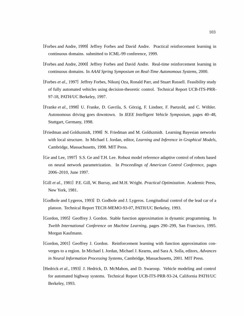
103

[Forbes and Andre, 1999] Jeffrey Forbes and David Andre. Practical reinforcement learning in

continuous domains. submitted to ICML-99 conference, 1999.

[Forbes and Andre, 2000] Jeffrey Forbes and David Andre. Real-time reinforcement learning in

continuous domains. In AAAI Spring Symposium on Real-Time Autonomous Systems, 2000.

[Forbes et al., 1997] Jeffrey Forbes, Nikunj Oza, Ronald Parr, and Stuart Russell. Feasibility study

of fully automated vehicles using decision-theoretic control. Technical Report UCB-ITS-PRR-

97-18, PATH/UC Berkeley, 1997.

[Franke et al., 1998] U. Franke, D. Gavrila, S. Gorzig, F. Lindner, F. Paetzold, and C. Wohler.

Autonomous driving goes downtown. In IEEE Intelligent Vehicle Symposium, pages 40–48,

Stuttgart, Germany, 1998.

[Friedman and Goldszmidt, 1998] N. Friedman and M. Goldszmidt. Learning Bayesian networks

with local structure. In Michael I. Jordan, editor, Learning and Inference in Graphical Models,

Cambridge, Massachusetts, 1998. MIT Press.

[Ge and Lee, 1997] S.S. Ge and T.H. Lee. Robust model reference adaptive control of robots based

on neural network parametrization. In Proceedings of American Control Conference, pages

2006–2010, June 1997.

[Gill et al., 1981] P.E. Gill, W. Burray, and M.H. Wright. Practical Optimization. Academic Press,

New York, 1981.

[Godbole and Lygeros, 1993] D. Godbole and J. Lygeros. Longitudinal control of the lead car of a

platoon. Technical Report TECH-MEMO-93-07, PATH/UC Berkeley, 1993.

[Gordon, 1995] Geoffrey J. Gordon. Stable function approximation in dynamic programming. In

Twelth International Conference on Machine Learning, pages 290–299, San Francisco, 1995.

Morgan Kaufmann.

[Gordon, 2001] Geoffrey J. Gordon. Reinforcement learning with function approximation con-

verges to a region. In Michael I. Jordan, Michael J. Kearns, and Sara A. Solla, editors, Advances

in Neural Information Processing Systems, Cambridge, Massachusetts, 2001. MIT Press.

[Hedrick et al., 1993] J. Hedrick, D. McMahon, and D. Swaroop. Vehicle modeling and control

for automated highway systems. Technical Report UCB-ITS-PRR-93-24, California PATH/UC

Berkeley, 1993.

104

[Hernandez-Gardiol and Mahadevan, 2000] Natalia Hernandez-Gardiol and Sridhar Mahadevan.

Hierarchical memory-based reinforcement learning. In Advances in Neural Information Pro-

cessing, volume 13, 2000.

[Howard, 1960] R. A. Howard. Dynamic Programming and Markov Processes. MIT Press, Cam-

bridge, Massachusetts, 1960.

[Jochem, 1996] Todd M. Jochem. Vision Based Tactical Driving. PhD thesis, Carnegie Mellon

University, 1996.

[Kaelbling et al., 1996] Leslie P. Kaelbling, Michael L. Littman, and Andrew W. Moore. Rein-

forcement learning: A survey. Journal of Artificial Intelligence Research, 4:237–285, 1996.

[Kaelbling et al., 1998] Leslie Pack Kaelbling, Michael L. Littman, and Anthony R. Cassandra.

Planning and acting partially observable domains. Artificial Intelligence, 101, 1998.

[Kearns et al., 1999] Michael Kearns, Y. Mansour, and Andrew Ng. Approximate planning in large

pomdps via reusable trajectories. In Advances in Neural Information Processing Systems, vol-

ume 12, 1999.

[Kibler and Aha, 1988] D. Kibler and D. W. Aha. Comparing instance-averaging with instance-

filtering algorithms. In Third European Working Session on Learning, pages 63–80, Glasgow,

Scotland, 1988. Pitman.

[Kirk, 1970] D. Kirk. Optimal Control Theory - An Introduction. Prentice-Hall, Englewood Cliffs,

New Jersey, 1970.

[Kirkpatrick et al., 1983] S. Kirkpatrick, C. D. Gelatt Jr., and M. P. Vecchi. Optimization by simu-

lated annealing. Scuebce, 220(4598):671–680, 1983.

[Kohonen, 1990] T. Kohonen. The self-organizing map. Proceedings of the IEEE, 78:1464–1480,

1990.

[Kruger et al., 1995] W. Kruger, W. Enkelmann, and S. Rossle. Real-time estimation and tracking

of optical flow vectors for obstacle detection. In IEEE Intelligent Vehicle Symposium, pages

341–346, Detroit, MI, 1995.

[Kumar and Varaiya, 1986] P.R. Kumar and Pravin Varaiya. Stochastic systems: Estimation, iden-

tification, and adaptive control. Prentice-Hall, Englewood Cliffs, New Jersey, 1986.

105

[Littman et al., 1995] Michael L. Littman, Thomas L. Dean, and Leslie Pack Kaelbling. On the

complexity of solving markov decision problems. In Eleventh Annual Conference on Uncertainty

in Artificial Intelligence, Montreal, Quebec, Canada, 1995.

[Lovejoy, 1993] William S. Lovejoy. A survey of algorithmic methods for partially observable

markov decision processes. Annals of Operations Research, 28:47–66, 1993.

[Luong et al., 1995] Q.-T. Luong, J. Weber, D. Koller, and J. Malik. An integrated stereo-based

approach to automatic vehicle guidance. In 5th ICCV, June 1995.

[Lutzeler and Dickmanns, 1998] M. Lutzeler and E. D. Dickmanns. Road recognition in marveye.

In IEEE Intelligent Vehicle Symposium, pages 341–346, Stuttgart, Germany, 1998.

[Lygeros et al., 1997] John Lygeros, Datta N. Godbole, and Shankar S. Sastry. A verified hy-

brid controller for automated vehicles. Technical Report UCB-ITS-PRR-97-9, California PATH,

1997.

[Malik et al., 1997] Jitendra Malik, Camillo J. Taylor, Philip McLauchlan, and Jana Kosecka. De-

velopment of binocular stereopsis for vehicle lateral control, longitudinal control and obstacle

detection. Technical report, UCB Path, 1997. Final Report MOU257.

[Mataric, 1991] Maja J. Mataric. A comparative analysis of reinforcement learning methods. Tech-

nical Report 1322, M.I.T. AI Lab, 1991.

[McCallum, 1995] Andrew Kachites McCallum. Reinforcement Learning with Selective Perception

and Hidden State. PhD thesis, University of Rochester, December 1995.

[Menger, 1956] K. Menger. What is calculus of variations and what are its applications? The World

of Mathematics, 2, 1956.

[Metropolis et al., 1953] N. Metropolis, A. Rosenbluth, M. Rosenbluth, A. Teller, and E. Teller.

Equations of state calculations by fast computing machines. Journal of Chemical Physics,

21:1087–1091, 1953.

[Meyer, 1995] Marjorie Teetor Meyer. One Man’s Vision: The Life of Automotive Pioneer Ralph

R. Teetor. Guild Press of Indiana, 1995.

[Middleton and Goodwin, 1990] R. H. Middleton and G. C. Goodwin. Digital Control and Esti-

mation, a Unified Approach. Prentice-Hall, 1990.

106

[Mitchell, 1997] Tom Mitchell. Machine Learning. McGraw-Hill, 1997.

[Moore and Atkeson, 1993] Andrew W. Moore and Christopher G. Atkeson. Prioritized sweeping–

reinforcement learning with less data and less time. Machine Learning, 13:103–130, 1993.

[Moore et al., 1997] Andrew W. Moore, C. G. Atkeson, and S. A. Schaal. Locally weighted learn-

ing for control. AI Review, 11:75–113, 1997.

[Moore, 1991] Andrew W. Moore. An introductory tutorial on kd-trees. Technical Report 209,

Computer Laboratory, University of Cambridge, 1991. Extract from A. W. Moore’s Phd. thesis:

Efficient Memory-based Learning for Robot Control.

[NAHSC, 1995] Current avcs deployment. Technical report, National Automated Highway System

Consortium, 1995. Located at http://ahs.volpe.dot.gov/avcsdoc/inuse.html.

[Narendra and Parthasarathy, 1991] K. Narendra and K. Parthasarathy. Gradient methods for the

optimisation of dynamical systems containing neural networks. IEEE Transactions on Neural

networks, 2:252–262, 1991.

[Ng and Jordan, 2000] Andrew Y. Ng and Michael I. Jordan. Pegasus: A policy search method for

large mdps and pomdps. In Uncertainty in Artificial Intelligence, 2000.

[Nise, 2000] Norman S. Nise. Control Systems Engineering. Benjamin/Cummings, 3 edition, 2000.

[Ormoneit and Hastie, 2000] Dirk Ormoneit and Trevor Hastie. Optimal kernel shapes for local

linear regression. In Sara A. Solla, Todd K. Leen, and Klaus-Robert Muller, editors, Advances

in Neural Information Processing Systems 12, pages 540–546, Cambridge, Massachusetts, 2000.

MIT Press.

[Ormoneit and Sen, 1999] Dirk Ormoneit and Saunak Sen. Kernel-based reinforcement learning.

Technical Report 1999-8, Department of Statistics, Stanford University, 1999.

[Papavassiliou and Russell, 1999] Vassilis Papavassiliou and Stuart Russell. Covergence of rein-

forcement learning with general function approximators. In International Joint Conference on

Artificial Intelligence, 1999.

[Parr and Russell, 1998] Ronald Parr and Stuart Russell. Reinforcement learning with hierarchies

of machines. In Michael Kearns, editor, Advances in Neural Information Processing Systems 10.

MIT Press, Cambridge, Massachusetts, 1998.

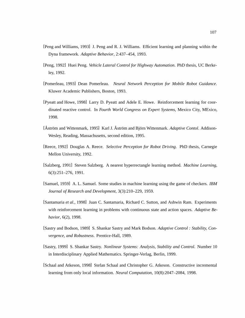
107

[Peng and Williams, 1993] J. Peng and R. J. Williams. Efficient learning and planning within the

Dyna framework. Adaptive Behavior, 2:437–454, 1993.

[Peng, 1992] Huei Peng. Vehicle Lateral Control for Highway Automation. PhD thesis, UC Berke-

ley, 1992.

[Pomerleau, 1993] Dean Pomerleau. Neural Network Perception for Mobile Robot Guidance.

Kluwer Academic Publishers, Boston, 1993.

[Pyeatt and Howe, 1998] Larry D. Pyeatt and Adele E. Howe. Reinforcement learning for coor-

dinated reactive control. In Fourth World Congress on Expert Systems, Mexico City, MExico,

1998.

[Astrom and Wittenmark, 1995] Karl J. Astrom and Bjorn Wittenmark. Adaptive Contol. Addison-

Wesley, Reading, Massachusetts, second edition, 1995.

[Reece, 1992] Douglas A. Reece. Selective Perception for Robot Driving. PhD thesis, Carnegie

Mellon University, 1992.

[Salzberg, 1991] Steven Salzberg. A nearest hyperrectangle learning method. Machine Learning,

6(3):251–276, 1991.

[Samuel, 1959] A. L. Samuel. Some studies in machine learning using the game of checkers. IBM

Journal of Research and Development, 3(3):210–229, 1959.

[Santamaria et al., 1998] Juan C. Santamaria, Richard C. Sutton, and Ashwin Ram. Experiments

with reinforcement learning in problems with continuous state and action spaces. Adaptive Be-

havior, 6(2), 1998.

[Sastry and Bodson, 1989] S. Shankar Sastry and Mark Bodson. Adaptive Control : Stability, Con-

vergence, and Robustness. Prentice-Hall, 1989.

[Sastry, 1999] S. Shankar Sastry. Nonlinear Systems: Analysis, Stability and Control. Number 10

in Interdisciplinary Applied Mathematics. Springer-Verlag, Berlin, 1999.

[Schaal and Atkeson, 1998] Stefan Schaal and Christopher G. Atkeson. Constructive incremental

learning from only local information. Neural Computation, 10(8):2047–2084, 1998.

108

[Schaal et al., 2000] Stefan Schaal, Chris Atkeson, and Sethu Vijayakumar. Scalable locally

weighted statistical techniques for real time robot learning. Scalable Robotic Applications of

Neural Networks - Special issue of Applied Intelligence, 2000.

[Schell and Dickmanns, 1994] F.R. Schell and E.D. Dickmanns. Autonomous landing of airplanes

by dynamic machine vision. MVA, 7(3):127–134, 1994.

[Singh and Sutton, 1996] Satinder Singh and R.S. Sutton. Reinforcement learning with replacing

eligibility traces. Machine Learning, 22:123–158, 1996.

[Singh, 1992] Satinder Singh. Reinforcement learning with hierarchies of machines. In Proceed-

ings of the Tenth National Conference on Artificial Intelligence (AAAI-92), San Jose, California,

July 1992. AAAI Press.

[Smart and Kaelbling, 2000] William D. Smart and Leslie Pack Kaelbling. Practical reinforcement

learning in continuous spaces. In Seventeenth International Conference on Machine Learning,

2000.

[Smart, 2002] William Smart. Making Reinforcement Learning Work on Real Robots. PhD thesis,

Brown University, 2002.

[Smola and Scholkopf, 1998] Alex J. Smola and Bernhard Scholkopf. A tutorial on support vec-

tor regression. Technical Report NC2-TR-1998-030, ESPIRIT Working Group in Neural and

Computational Learning 2, October 1998.

[Sukthankar et al., 1995] R. Sukthankar, D. Pomerleau, and C. Thorpe. Shiva: Simulated highways

for intelligent vehicle algorithms. In IEEE IV, 1995.

[Sukthankar, 1995] Rahul Sukthankar. Situational Awareness for Driving in Traffic. PhD thesis,

Carnegie Mellon University, 1995.

[Sutton and Barto, 1998] Richard S. Sutton and Andrew G. Barto. Reinforcement Learning: An

Introduction. MIT Press, Cambridge, MA, 1998.

[Sutton and Santamaria, 1998] Richard S. Sutton and Juan Carlos Santamaria. A Standard In-

terface for Reinforcement Learning Software, 1998. See homepage at http://www-

anw.cs.umass.edu/ rich/RLinterface.html.

109

[Sutton et al., 1998] Richard S. Sutton, Satinder Singh, Doina Precup, and Balaraman Ravindran.

Improved switching among temporally abstract actions. In Advances in Neural Information Pro-

cessing Systems, volume 11, 1998.

[Sutton, 1990] R. S. Sutton. First results with DYNA, an integrated architecture for learning, plan-

ning, and reacting. In Proceedings of the Eighth National Conference on Artificial Intelligence

(AAAI-90), Boston, Massachusetts, 1990. MIT Press.

[Tadepalli and Ok, 1996] Prasad Tadepalli and DoKyeong Ok. Scaling up average reward reinfor-

cmeent learning by approximating the domain models and the value function. In Proceedings

of the Thirteenth International Conference on Machine Learning, Bari, Italy, July 1996. Morgan

Kaufmann.

[Taylor et al., 1999] Camillo J. Taylor, Jana Kosecka, Roberto Blasi, and Jittendra Malik. A com-

parative study of vision-based lateral control strategies for autonomous highway driving. Inter-

national Journal of Robotics Research, 18(5):442–453, 1999.

[Tesauro, 1992] G. Tesauro. Practical issues in temporal difference learning. Machine Learning,

8(3–4):257–277, May 1992.

[Thrun and Schwartz, 1993] Sebastian Thrun and Anton Schwartz. Issues in using function approx-

imation for reinforcement learning. In Fourth Connectionist Models Summer School, Hillsdale,

NJ, 1993. Lawrence Erlbaum.

[Thrun et al., 2000] S. Thrun, D. Fox, W. Burgard, and F. Dellaert. Robust monte carlo localization

for mobile robots. Artificial Intelligence, 101:99–141, 2000.

[Time, 1994] Time, editor. Time Almanac: Reference Edition. Compact Publishing Co., 1994.

[Tokuyama, 1997] H. Tokuyama. Asia-pacific projects status and plans. In International AHS

Workshop. US Department of Transportation, 1997.

[Tomizuka et al., 1995] M. Tomizuka, J.K. Hedrick, and H. Pham. Integrated manuevering control

for automated highway system based on a magnetic reference/sensing system. Technical Report

UCB-ITS-PRR-95-12, California PATH/UC Berkeley, 1995.

[Trivedi, 1989] M.M. Trivedi. Designing vision systems for robotic applications. SPIE, xx:106–

115, January 1989.

110

[Tsitsiklis and Van Roy, 1997] John N. Tsitsiklis and Benjamin Van Roy. An analysis of temporal-

difference learning with function approximation. In IEEE Transactions on Automatic Control,

volume 42, pages 674–690, 1997.

[Varaiya, 1991] Pravin Varaiya. Smart cars on smart roads: Problems of control. Technical report,

California PATH/UC Berkeley, 1991.

[Vijayakumar and Schaal, 2000] Sethu Vijayakumar and Stefan Schaal. Real time learning in hu-

manoids: A challenge for scalability of online algorithms. In Humanoids2000, First IEEE-RAS

International Conference on Humanoid Robots, 2000.

[Waltz, 1990] D. Waltz. Memory-based reasoning. In M. Arbib and J. Robinson, editors, Natural

and Artificial Parallel Compuatation, pages 251–276. MIT Press, Cambridge, Massachusetts,

1990.

[Weaver et al., 1998] Scott Weaver, Leemon Baird, and Marios Polycarpou. Preventing unlearn-

ing during on-line training of feedforward networks. In International Symposium of Intelligent

Control, Gaithersburg, MD, September 1998.

[Wellman et al., 1995] Michael P. Wellman, Chao-Lin Liu, David Pynadath, Stuart Russell, Jeffrey

Forbes, Timothy Huang, and Keiji Kanazawa. Decision-theoretic reasoning for traffic monitoring

and vehicle control. In IEEE IV, 1995.

[Whitley et al., 2000] D. Whitley, David Goldberg, Erick Cantu-Paz, Lee Spector, Ian Parmee, and

Hans-Georg Beyer, editors. GECCO - Genetic and Evolutionary Computation Conference, Las

Vegas, NV, 2000. Morgan Kaufmann.

[Witten, 1977] I. H. Witten. An adaptive optimal controller for discrete-time markov environments.

Information and Control, 34:286–295, 1977.

[Zhang and Dietterich, 1996] W. Zhang and T.G. Dietterich. High-performance job-shop schedul-

ing with a time delay TD(>) network. In D.S. Touretzky, M. C. Mozer, and M. E. Hasselmo,

editors, Advances of Neural Information Processing Systems, volume 8, pages 1024–1030, Cam-

bridge, Massachusetts, 1996. MIT Press.

Documents

Reinforcement Learning for Autonomous Vehicles