relating water productivity and crop evapotranspiration

OPTIONS méditerranéennes Series B, n° 57

RELATING WATER PRODUCTIVITY AND CROP EVAPOTRANSPIRATION

L.S. Pereira Center for Agricultural Engineering Research, Institute of Agronomy,

Technical University of Lisbon, Tapada da Ajuda, 1349-017 Lisbon, Portugal, Fax: +351 21 362 1575; E-mail: [email protected]

SUMMARY - Water productivity became an important issue in improving the performance of irrigation, including when focusing water saving issues. However, various concepts may be considered, which requires appropriate definitions and related analysis. Because it represents a ratio between harvesting yield and water use, a main component of the latter is crop evapotranspiration. This calls for a discussion relative to its concepts and computation, thus to identify both how crop evapotranspiration may be managed to improve water productivity and existing gaps in its knowledge. In addition, a discussion on the economic aspects relative to improved water productivity and saving is presented, including a simple analysis of economic issues and respective gaps in knowledge. Key words: water productivity, land productivity, evapotranspiration, aerodynamic resistance, surface resistance, crop coefficients, stress coefficients. WATER PRODUCTIVITY VS. IRRIGATION EFFICIENCY

The term efficiency is commonly applied an irrigation systems or sub-system: water storage,

conveyance, distribution off- and on-farm, and application at the farm. It can be defined by the ratio between the water depth delivered by the sub-system under consideration and the water depth supplied to that sub-system, usually expressed as a percentage. Adopting an output/input non-dimensional ratio, the term efficiency could be applied to evaluate the performance of any irrigation and non-irrigation water system but the term is almost exclusive of irrigation (Pereira et al., 2002a). Misleading interpretations are therefore common by water managers, which should be avoided.

For farm irrigation systems, the application efficiency Ea may be defined by the ratio between the

average water depth added to the root zone storage in the quarter of the field receiving less water to the average water applied. However, this indicator should be used together with others, mainly those relative to distribution uniformity (Burt et al., 1997; Pereira, 1999; Pereira and Trout, 1999). Moreover, this indicator Ea should not be used for characterizing seasonal irrigation but only each irrigation event because soil water availability and water depths applied vary from an irrigation to the next and they highly influence this performance indicator as analysed by those authors. In addition, weather conditions, mainly wind speed and temperature in case of sprinkler irrigation, may also vary from an irrigation event to another and largely influence Ea.

Farmers do not see the improvement of farm application efficiencies as a must. Application

efficiencies become higher when farmers apply water timely and the distribution uniformity is higher. Improved uniformities decrease differences in amounts of water made available for the crop in the under-and over-irrigated parts of the field. As discussed by many authors, e.g. Keller and Bliesner (1990) and Mantovani et al. (1995), this leads to more even crop development and higher yields. When the farmer adopts an appropriate irrigation scheduling, then yields are positively impacted; in addition, the application efficiency becomes higher as well as the economic results of irrigation (Ortega et al., 2005). Thus, improving irrigation efficiency is not a farmer’s objective but to achieve higher yields and economic profit.

Improving transport and distribution efficiencies may be an objective of farmers management of

irrigation systems when seepage, leaking or overflow would decrease the availability of water to tail-end distributor canals and tail-end farmers, or when improvements aim at an easier control of deliveries to branch canals, distributors and farms. In other words, the interest of farmers is to have

31


improved service performances. Thus, the former efficiency terms are being replaced by indicators of canal and pipe systems that refer to service performance, such as reliability, dependability and equity (Molden and Gates, 1990; Lamaddalena and Pereira, 1998; Lamaddalena and Sagardoy, 2000; Pereira et al., 2003a; Bos et al., 2005).

Improving irrigation efficiencies is often said to be an objective associated with water savings.

However this is only true when the farmers and canal managers have the appropriate tools and farm and off farm irrigation systems are designed and managed in such a way that delivery and irrigation scheduling can be applied effectively, as discussed by Pereira et al. (2002a, b). Otherwise water savings may not be achieved in that way but through under-irrigating the crop.

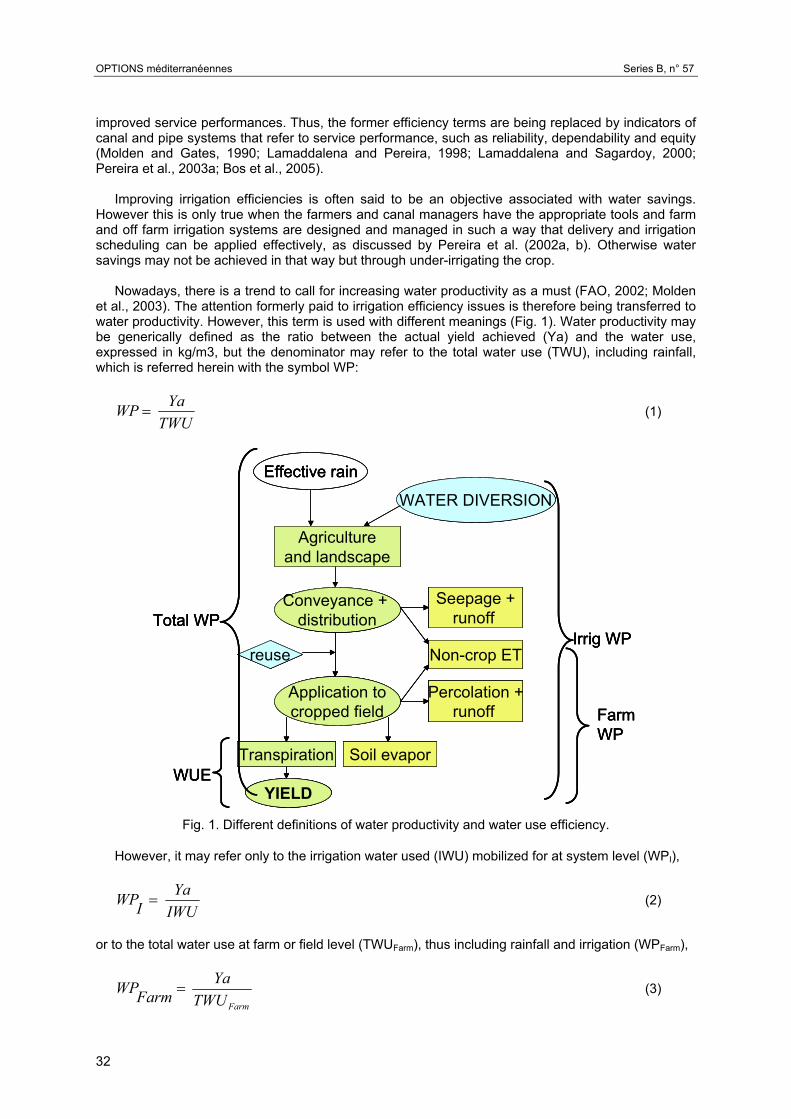
Nowadays, there is a trend to call for increasing water productivity as a must (FAO, 2002; Molden

et al., 2003). The attention formerly paid to irrigation efficiency issues is therefore being transferred to water productivity. However, this term is used with different meanings (Fig. 1). Water productivity may be generically defined as the ratio between the actual yield achieved (Ya) and the water use, expressed in kg/m3, but the denominator may refer to the total water use (TWU), including rainfall, which is referred herein with the symbol WP:

TWUYaWP = (1)

WATER DIVERSION

Agricultureand landscape

Effective rain

Transpiration Soil evapor

Seepage +runoff

Conveyance + distribution

Application tocropped field

Percolation +runoff

Non-crop ET

YIELD

reuse

Total WPIrrig WP

WUE

Farm WP

WATER DIVERSION


Effective rain


Seepage +runoff



Percolation +runoff

Non-crop ET

YIELD

reuse

WATER DIVERSION


Effective rain


Seepage +runoff



Percolation +runoff

Non-crop ET

YIELD

reuse


Seepage +runoff



Percolation +runoff

Non-crop ET

YIELD

reuse

Total WPTotal WPIrrig WPIrrig WP

WUEWUE

Farm WPFarm WP

Fig. 1. Different definitions of water productivity and water use efficiency.

However, it may refer only to the irrigation water used (IWU) mobilized for at system level (WPI),

IWUYa

IWP = (2)

or to the total water use at farm or field level (TWUFarm), thus including rainfall and irrigation (WPFarm),

FarmTWUYa

FarmWP = (3)

32


or relate to irrigation water (IWUFarm) only, thus (WPI-Farm):

FarmIWUYa

FarmIWP =− (4)

The meaning of these indicators is necessarily different and may cause contradictions when the

wording water productivity is used without specifying which target is being considered. The term water use efficiency (WUE) is also commonly used in irrigation but often with different

meanings. Some authors refer to it as a synonymous of application efficiency, thus as a non-dimensional output/input ratio; others adopt it to express the water productivity of the irrigation water, as a yield to water ratio. To avoid misunderstandings, the term water use efficiency should be limited to physiological and eco-physiological purposes (Steduto, 1996) or, as some do, may be replaced by the term transpiration ratio or similar.

The idea that improving water productivity or the water use efficiency leads to water savings is also

not entirely true because it is also required to distinguish between consumptive and non-consumptive uses. The same amount of grain yield depends not only on the amount of irrigation water used but also on the amount of rainfall water that the crop could use, which relates to rainfall distribution during the crop season. Moreover, the pathways to improve yields are often not related with water management but with agronomic practices and the adaptation of the crop variety to the cropping environment. However, a crop variety that has a higher WUE than another has the potential for using less water than the second when achieving the same yield. But this is a characteristic intrinsic to the crop and is not depending upon irrigation management.

WATER PRODUCTIVITY CONCEPTS Considering Fig. 1, one may approach the different concepts relative to water productivity and

assume some definitions aimed at irrigation management. Then the following base definition is adopted:

TWUYaWP = (1a)

where Ya is the actual harvestable yield in kg, and TWU is the total seasonal water use by the crop in m3 or, referring to the unit surface, in mm.

Eq. 1a may take a different form

NBWULFETaYaWP++

= (5)

where Ya is the actual harvestable yield and the denominator refers to the water use components; ETa is the actual season evapotranspiration in mm, LF is the water used for leaching in mm and NBWU is the non-beneficial water use in mm. This concerns the percolation through the bottom of the root zone, runoff out of the irrigated fields, and losses by evaporation and wind drift, The beneficial water use (BWU) is then constituted of ETa and LF.

If the seasonal water use is considered through the respective and diverse water sources, then Eq.

5 is replaced by the following equation:

ISWCRPYaWP

+∆++= (6)

33


where P is the season precipitation, CR is the amount of capillary rise, ∆SW is the difference in soil water content between planting and harvest and I is the seasonal irrigation depth, all expressed in mm.

One can observe that maximizing water productivity is to find out its limit when the maximal yield Ymax is attained, which means that ETa = ETc, where ETc is defined as the ET of a healthy crop, well managed and not short of water, thus cultivated under pristine conditions (Allen et al., 1998), and that NBWU is at its minimum value:

( ) ( )NBWULFETcYWP

minmaxmax++

= (7)

An high WP may also be obtained when a crop is water stressed (up to acceptable limits); then the

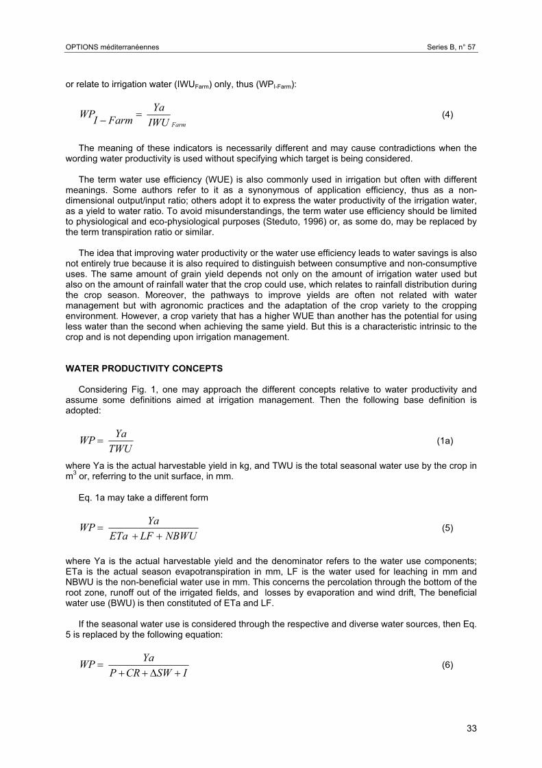
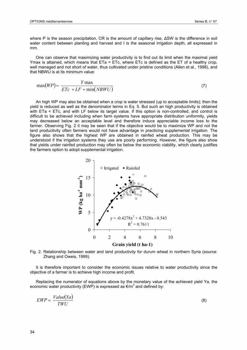
yield is reduced as well as the denominator terms in Eq. 5. But such an high productivity is obtained with ETa < ETc, and with LF below its target value. If this option is non-controlled, and control is difficult to be achieved including when farm systems have appropriate distribution uniformity, yields may decreased below an acceptable level and therefore induce appreciable income loss to the farmer. Observing Fig. 2 it may be seen that if the objective would be to maximize WP and not the land productivity often farmers would not have advantage in practicing supplemental irrigation. The figure also shows that the highest WP are obtained in rainfed wheat production. This may be understood if the irrigation systems they use are poorly performing. However, the figure also show that yields under rainfed production may often be below the economic viability, which clearly justifies the farmers option to adopt supplemental irrigation.

y = -0.4278x2 + 4.7328x - 0.543R2 = 0.7611

0

5

10

15

20

0 2 4 6 8 10Grain yield (t ha-1)

WP

(kg

ha-1

mm

-1)

Irrigated Rainfed

Fig. 2. Relationship between water and land productivity for durum wheat in northern Syria (source:

Zhang and Oweis, 1999). It is therefore important to consider the economic issues relative to water productivity since the

objective of a farmer is to achieve high income and profit. Replacing the numerator of equations above by the monetary value of the achieved yield Ya, the

economic water productivity (EWP) is expressed as €/m3 and defined by:

( )TWU

YaValueEWP = (8)

34


However, the economics of production is less visible in this form than when both the numerator

and the denominator are expressed in monetary (€) terms, respectively the yield value and the TWU cost, thus yielding the following definition:

( )( )TWUCostYaValueEWP = (9)

Alternatively, this definition may be expressed assuming that all water costs are due to the costs of irrigation, thus:

( )( )ICostSWCRP

YaValueEWP+∆++

= (10)

This may not be true if water conservation measure are used and therefore there are costs associated with water harvesting or soil management that create additional mobilization of rainfall, mainly increasing the infiltrated fraction and/or reducing soil water evaporation losses. Alternatively, considering Eq. 5, the following definition may be used:

( )( )NBWULFETaCosts

YaValueEWP++

= (11)

Determining the costs associated with the water use components as in Eq. 11 may be difficult but

ideally this equation may support the economic evaluation of measures to control the NBWU. Maximizing EWP, when all costs not referring to water use are kept constant, means to find the

limit to the ratio between the yield value and the yield costs associated with water use, which corresponds to maximize the crop revenue in which concerns water use:

( ) ( ) (IncomeYCostsYValueEWP max

max)(maxmaxmax == ) (12)

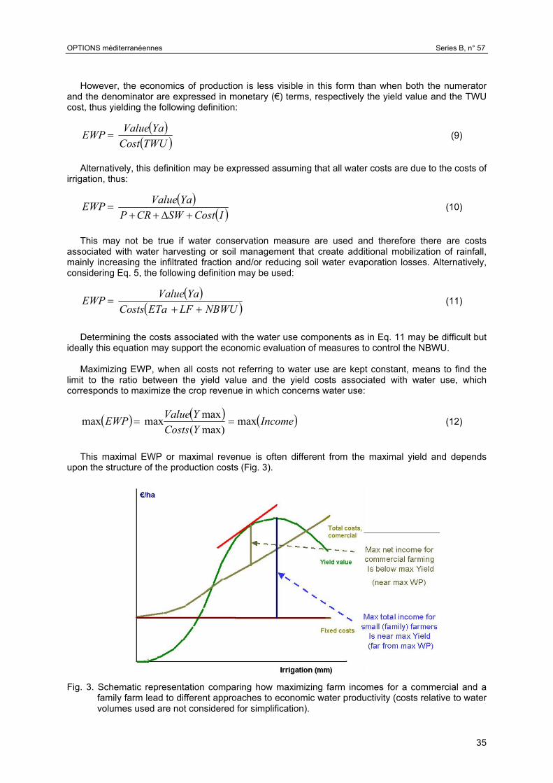
This maximal EWP or maximal revenue is often different from the maximal yield and depends

upon the structure of the production costs (Fig. 3).

Fig. 3. Schematic representation comparing how maximizing farm incomes for a commercial and a

family farm lead to different approaches to economic water productivity (costs relative to water volumes used are not considered for simplification).

35


For a farm where labour is by workers or using somewhat sophisticated equipment associated with

energy costs, then the irrigation costs grow almost linearly with the amount of irrigation water use. Contrarily, for a farm using surface irrigation without energy costs associated nor large capital investment, and where labour is provided by the family, thus is remunerated by the final yield, the effective costs relative to irrigation are not depending upon the amount of irrigation water use. Therefore, the maximum net income for the first may be close to the maximal EWP, while the maximum income for the family farm are close to the maximal land productivity since land, not water, is the main limiting factor determining farm income. The related economic impacts are however less well known, insufficient data are available and tools for the respective analysis are insufficiently developed (Victoria et al., 2005).

It is therefore important to understand how WP could be improved. Knowing that yields depend

upon the seasonal evapotranspiration, this analysis focuses this component of the water use.

Crop Evapotranspiration and resistances to vapour fluxes

The Penman-Monteith equation (Monteith, 1965) is generally considered to be able to represent the evapotranspiration from any vegetated surface (Jensen et al., 1990; Allen et al., 1994, 1998; Pereira et al., 1999). It can be expressed by the following combination equation:

++∆

−+−∆

=

a

s

a

aspan

rr1

r)e(ecG)(R

ETγ

ρλ (13)

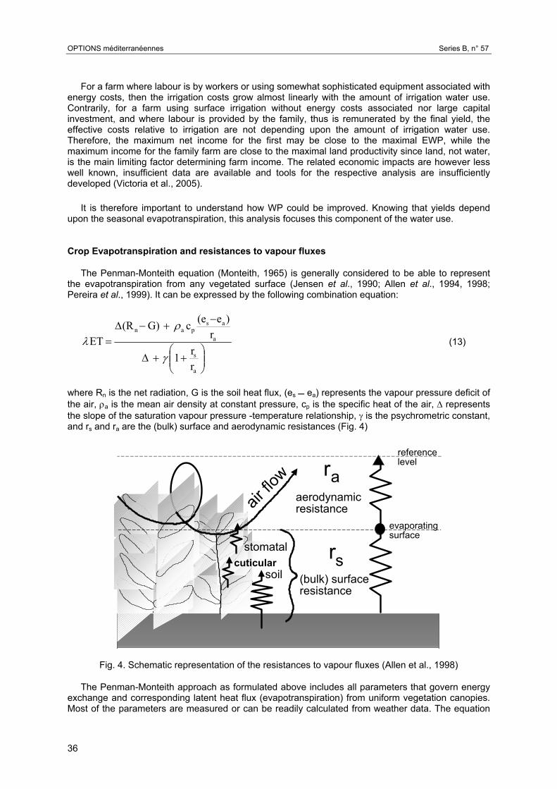
where Rn is the net radiation, G is the soil heat flux, (es ea) represents the vapour pressure deficit of the air, ρa is the mean air density at constant pressure, cp is the specific heat of the air, ∆ represents the slope of the saturation vapour pressure -temperature relationship, γ is the psychrometric constant, and rs and ra are the (bulk) surface and aerodynamic resistances (Fig. 4)

soil

stomatal

air flo

w

r

r

s

a

(bulk) surface resistance

aerodynamicresistance

referencelevel

evaporatingsurface

cuticular

Fig. 4. Schematic representation of the resistances to vapour fluxes (Allen et al., 1998)

The Penman-Monteith approach as formulated above includes all parameters that govern energy exchange and corresponding latent heat flux (evapotranspiration) from uniform vegetation canopies. Most of the parameters are measured or can be readily calculated from weather data. The equation

36


can be utilized for the direct calculation of any crop evapotranspiration as the surface and aerodynamic resistances are crop specific.

Aerodynamic resistance (ra) determines the transfer of heat and water vapour from the evaporating surface into the air above the canopy. It can be expressed as:

( )[ ] ( )[ ]z

mha uk

zdzzdzr 2omoH /ln/ln −−

= (14)

where ra is the aerodynamic resistance [s m-1], zm is height of wind measurements [m], zh is the height of air humidity measurements [m], d is the zero plane displacement height [m], zom is the roughness length governing momentum transfer [m], zoh is the roughness length governing transfer of heat and vapour [m], k is the von Karman's constant, 0.41 [-], and uz is the wind speed at height z [m s-1].

As discussed by Alves et al. (1998), the assumption that heat and vapour escape from the canopy from the level d+zoH, as it is implied in Eq. 14, can be questioned. In alternative, ra can be calculated from the top of the canopy to the reference height, using (Perrier, 1975; Stockle and Kjelgaard, 1996):

( ) ( )[ ] ( )[ ]z

mcha uk

zdzdhdzr 2om/ln/ln −−−

= (15)

where hc is the crop height [m].

These equations are restricted for neutral stability conditions, i.e., where temperature, atmospheric pressure, and wind velocity distributions follow nearly adiabatic conditions (no heat exchange). The application of the ra equations for short time periods (hourly or less) may require the inclusion of corrections for stability. However, when predicting ETo in the well-watered reference surface, heat exchanged is small, and therefore stability correction is normally not required.

For its practical application, the parameters d and zo, if not measured, can be estimated from the crop height hc [m] and LAI [-] (e.g. Brutsaert, 1982; Perrier, 1982):

((

−−−= 2121 /LAIexp

LAIhd c ))

]

(16)

( )[ )/LAIexp(/LAIexphz com 212 −−−= (17)

Genetic improvements and crop management influence these parameters through acting on hc [m] and LAI but impacts are relatively small. Aiming at increasing WP (Eqs. 5 and 7) changes should focus on decreasing ETa and ETc, thus on increasing the aerodynamic resistance, thus decreasing both d and zom (vd. Eqs. 14 and 15); however the main impact on ra depends on weather conditions through wind speed. Eqs. 16 and 17 show that d and zom increase for high and fully cover crops and are smaller for low crop heights and partial cover crops. Thus, plant breeding improvements may favour higher ra when crops become lower in height and LAI.

Surface resistance is more complex. The ‘bulk’ surface resistance describes the resistance of

vapour flow through the transpiring crop and evaporating soil surface. Where the vegetation does not completely cover the soil, the resistance factor should indeed include the effects of the evaporation from the soil surface. If the crop is not transpiring at a potential rate, the resistance depends also on the water status of the vegetation.

Plant physiologists consider rs to be a purely physiological parameter that accounts for the stomatal control of transpiration. Stomata have been carefully studied and the factors that determine their functioning are well known. Some of them, like radiation, either solar radiation Rn or PAR, temperature (T) and vapour pressure deficit (VPD) are those that govern the physical process of evaporation. Others, like soil (or plant) water potential (ψ ) represent the true physiological control by

37


stomata which takes place mainly in water stress conditions. Other factors, like the age of the leaf, the previous history of water stress of the plant and the position of the leaf in the plant, are also important but less quantifiable (Alves and Pereira, 2000).

Scaling resistances from leaf to canopy, which constitutes the "bottom up" approach to rs, is full of controversy. The standard procedure is to average stomatal resistance rst at different levels in the canopy, weighted by leaf area index (Monteith, 1973). However, the values of rs determined this way even with measured stomatal resistances seem to give good results only in very rough surfaces, like forests, and partial cover crops with a dry soil. On complete cover crops, especially when the soil is wet, average stomatal resistance can greatly depart, being normally lower, from the values of rs obtained as a residual term of the Penman-Monteith equation using the "top down" approach (e.g. Baldocchi et al., 1991; Rochette et al., 1991). The following equation establishes the essential relations between rs and weather variables (Alves and Pereira, 2000):

( ) ( )GRVPDc

rrn

paas −

++

−

∆=

γρ

ββγ

11 (18)

where ∆ is the slope of the vapour pressure curve (Pa/ºC), γ is the psychrometric constant (Pa/ºC), ρa is the atmospheric density (kg/m3), cp is the specific heat of moist air (J kg-1 ºC-1), Rn-G is the energy available at the crop surface, and β is the Bowen ratio. This discrepancy has been regarded as to indicate that not all leaves actually contribute to the total evaporation fluxes from the canopy. The concept of "effective" leaf area was therefore introduced and linked to radiation interception, the upper, well illuminated leaves being those that most contribute to transpiration.

The surface resistance rs is crop specific and relates to the stomatal resistance rst and to the "effective" leaf area; increasing resistance to water stress implies increased stomatal control, thus higher rst and rs. plant breeding for increased resistance to water stress may lead to increased rst and rs; however, acting on these crop characteristics is difficult and should avoid that increasing rst and rs would lead to lower photosynthetic efficiency, which would decrease WUE. Referring to Eq. 18, non considering the role of climate that may be the essential factor determining rs, it becomes evident that the main factor to act on is the Bowen ratio β: since it represents the ratio between sensible and latent heat fluxes, a low β indicates high water availability to the crop and an high β is representative of water stress conditions. Therefore, for unchanged climate conditions, high rs values are obtained when the aerodynamic resistance is high and the crop is water stressed. However, limiting the availability of water to the crop may lead to lowering the photosynthesis and to reduced yields. As for ra, acting on rs is difficult, could have contradictory results in terms of crop yields, and may be less efficient in increasing WP.

CROP EVAPOTRANSPIRATION AND CROP COEFFICIENTS Crop evapotranspiration can be derived from meteorological and crop data by means of the

Penman-Monteith equation (Eq. 13). By adjusting the albedo and the aerodynamic and canopy surface resistances to the growing characteristics of the specific crop, the evapotranspiration rate can be directly estimated. The albedo and resistances are, however, difficult to estimate accurately as they may vary continually during the growing season as climatic conditions change, as the crop develops, and with soil surface wetness and soil water availability. The canopy resistance will further be influenced by the soil water availability, and it increases strongly if the crop is subjected to water stress.

As there is still a considerable lack of consolidated information on the aerodynamic and canopy resistances for the various cropped surfaces, the crop coefficient approach is generally used to estimate the crop evapotranspiration, ETc, which is calculated by multiplying the reference crop evapotranspiration, ETo, by a crop coefficient, Kc:

occ ETKET = (19)

38


where ETc is the crop evapotranspiration [mm d-1], Kc is the crop coefficient [dimensionless], and ETo is reference crop evapotranspiration [mm d-1].

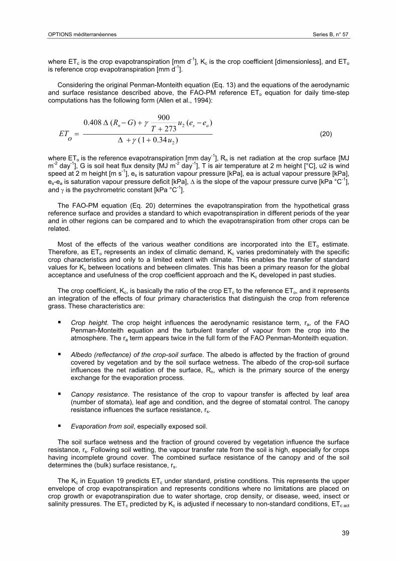
Considering the original Penman-Monteith equation (Eq. 13) and the equations of the aerodynamic and surface resistance described above, the FAO-PM reference ETo equation for daily time-step computations has the following form (Allen et al., 1994):

)34.01(

)(273

900)(408.0

2

2

u

eeuT

GR

oETasn

++∆

−+

+−∆=

γ

γ (20)

where ETo is the reference evapotranspiration [mm day-1], Rn is net radiation at the crop surface [MJ m-2 day-1], G is soil heat flux density [MJ m-2 day-1], T is air temperature at 2 m height [°C], u2 is wind speed at 2 m height [m s-1], es is saturation vapour pressure [kPa], ea is actual vapour pressure [kPa], es-ea is saturation vapour pressure deficit [kPa], ∆ is the slope of the vapour pressure curve [kPa °C-1], and γ is the psychrometric constant [kPa °C-1].

The FAO-PM equation (Eq. 20) determines the evapotranspiration from the hypothetical grass reference surface and provides a standard to which evapotranspiration in different periods of the year and in other regions can be compared and to which the evapotranspiration from other crops can be related.

Most of the effects of the various weather conditions are incorporated into the ETo estimate. Therefore, as ETo represents an index of climatic demand, Kc varies predominately with the specific crop characteristics and only to a limited extent with climate. This enables the transfer of standard values for Kc between locations and between climates. This has been a primary reason for the global acceptance and usefulness of the crop coefficient approach and the Kc developed in past studies.

The crop coefficient, Kc, is basically the ratio of the crop ETc to the reference ETo, and it represents an integration of the effects of four primary characteristics that distinguish the crop from reference grass. These characteristics are:

Crop height. The crop height influences the aerodynamic resistance term, ra, of the FAO Penman-Monteith equation and the turbulent transfer of vapour from the crop into the atmosphere. The ra term appears twice in the full form of the FAO Penman-Monteith equation.

Albedo (reflectance) of the crop-soil surface. The albedo is affected by the fraction of ground covered by vegetation and by the soil surface wetness. The albedo of the crop-soil surface influences the net radiation of the surface, Rn, which is the primary source of the energy exchange for the evaporation process.

Canopy resistance. The resistance of the crop to vapour transfer is affected by leaf area (number of stomata), leaf age and condition, and the degree of stomatal control. The canopy resistance influences the surface resistance, rs.

Evaporation from soil, especially exposed soil.

The soil surface wetness and the fraction of ground covered by vegetation influence the surface resistance, rs. Following soil wetting, the vapour transfer rate from the soil is high, especially for crops having incomplete ground cover. The combined surface resistance of the canopy and of the soil determines the (bulk) surface resistance, rs.

The Kc in Equation 19 predicts ETc under standard, pristine conditions. This represents the upper envelope of crop evapotranspiration and represents conditions where no limitations are placed on crop growth or evapotranspiration due to water shortage, crop density, or disease, weed, insect or salinity pressures. The ETc predicted by Kc is adjusted if necessary to non-standard conditions, ETc act

39


or ETa, where any environmental condition or characteristic is known to have an impact on or to limit ETc. For this reason, ETa is used when defining WP (Eq. 5) and ETc is used in Eq. 7 referring to the maximal WP. These aspects are represented in Fig. 5.

Actual ETc can be less than the potential ETc under non-potential growing conditions including water stress or high soil salinity. The non-potential ETc is termed “actual ETc” and is represented as ETc act. It is defined as:

oactcactc ETKET = (21)

where Kc act is the “actual” crop coefficient that includes effects of environmental stresses.

x =ET

ETKK

water & environmentalstress

s c adjusted c adj

o

x

RadiationTemperatureWind speedHumidity

climate

+ =

x =

well watered

well watered

grassreference

cropETo

ETo

ETcKc factor

grass

crop

conditionsoptimal agronomic

Yield = Ym

Yield = Ya

x =ET

ETKK


s c adjusted c adj

o

x


climate

+ =

x =

well watered

well watered

grassreference

cropETo

ETo

ETcKc factor

grass

crop


Yield = Ym

Yield = Ya

Yield = Ym

Yield = Yaactx =ET

ETKK


s c adjusted c adj

o

x


climate

+ =

x =

well watered

well watered

grassreference

cropETo

ETo

ETcKc factor

grass

crop


Yield = Ym

Yield = Ya

x =ET

ETKK


s c adjusted c adj

o

x


climate

+ =

x =

well watered

well watered

grassreference

cropETo

ETo

ETcKc factor

grass

crop


Yield = Ym

Yield = Ya

Yield = Ym

Yield = Ya

x =ET

ETKK


s c adjusted c adj

o

x


climate

+ =

x =

well watered

well watered

grassreference

cropETo

ETo

ETcKc factor

grass

crop


Yield = Ym

Yield = Ya

x =ET

ETKK


s c adjusted c adj

o

x


climate

+ =

x =

well watered

well watered

grassreference

cropETo

ETo

ETcKc factor

grass

crop


Yield = Ym

Yield = Ya

Yield = Ym

Yield = Yaact

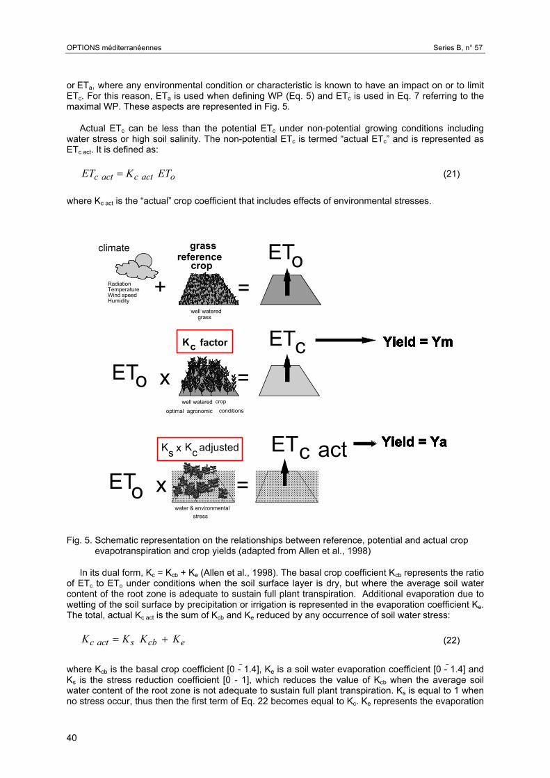
Fig. 5. Schematic representation on the relationships between reference, potential and actual crop evapotranspiration and crop yields (adapted from Allen et al., 1998)

In its dual form, Kc = Kcb + Ke (Allen et al., 1998). The basal crop coefficient Kcb represents the ratio of ETc to ETo under conditions when the soil surface layer is dry, but where the average soil water content of the root zone is adequate to sustain full plant transpiration. Additional evaporation due to wetting of the soil surface by precipitation or irrigation is represented in the evaporation coefficient Ke. The total, actual Kc act is the sum of Kcb and Ke reduced by any occurrence of soil water stress:

ecbsactc KKKK += (22)

where Kcb is the basal crop coefficient [0 - 1.4], Ke is a soil water evaporation coefficient [0 - 1.4] and Ks is the stress reduction coefficient [0 - 1], which reduces the value of Kcb when the average soil water content of the root zone is not adequate to sustain full plant transpiration. Ks is equal to 1 when no stress occur, thus then the first term of Eq. 22 becomes equal to Kc. Ke represents the evaporation

40


component from wet soil that occurs in addition to the ET represented in Kcb. The sum of Kcb and Ke can not exceed some maximum value for a crop, based on energy limitations, generally referred as the Kc. the value. An update and extension on the use of Eq. 22 is given by Allen et al. (2005a).

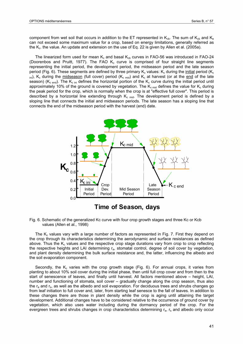
The linearized form used for mean Kc and basal Kcb curves in FAO-56 was introduced in FAO-24 (Doorenbos and Pruitt, 1977). The FAO Kc curve is comprised of four straight line segments representing the initial period, the development period, the midseason period and the late season period (Fig. 6). These segments are defined by three primary Kc values: Kc during the initial period (Kc

ini), Kc during the midseason (full cover) period (Kc mid) and Kc at harvest (or at the end of the late season) (Kc end). The Kc ini defines the horizontal portion of the Kc curve during the initial period until approximately 10% of the ground is covered by vegetation. The Kc mid defines the value for Kc during the peak period for the crop, which is normally when the crop is at "effective full cover". This period is described by a horizontal line extending through Kc mid. The development period is defined by a sloping line that connects the initial and midseason periods. The late season has a sloping line that connects the end of the midseason period with the harvest (end) date.

CropDev.Initial

PeriodPeriodPeriodPeriodMid Season

LateSeason

Time of Season, days

Kc

0.2

0.4

0.6

0.8

1.0

1.2

0.0

Kc ini

Kc mid

K c end

Fig. 6. Schematic of the generalized Kc curve with four crop growth stages and three Kc or Kcb values (Allen et al., 1998)

The Kc values vary with a large number of factors as represented in Fig. 7. First they depend on the crop through its characteristics determining the aerodynamic and surface resistances as defined above. Thus the Kc values and the respective crop stage durations vary from crop to crop reflecting the respective heights and LAI determining ra, stomatal control, degree of soil cover by vegetation, and plant density determining the bulk surface resistance and, the latter, influencing the albedo and the soil evaporation component.

Secondly, the Kc varies with the crop growth stage (Fig. 6). For annual crops, it varies from planting to about 10% soil cover during the initial phase, then until full crop cover and from then to the start of senescence of leaves, and finally until harvest. All factors mentioned above – height, LAI, number and functioning of stomata, soil cover – gradually change along the crop season, thus also the ra and rs, as well as the albedo and soil evaporation. For deciduous trees and shrubs changes go from leaf initiation to full cover and, later, from starting leaf senesce to the fall of leaves. In addition to these changes there are those in plant density while the crop is aging until attaining the target development. Additional changes have to be considered relative to the occurrence of ground cover by vegetation, which also uses water including during the dormancy period of the crop. For the evergreen trees and shrubs changes in crop characteristics determining ra, rs and albedo only occur

41


during the first years of the crop but the influences of ground cover are also non-negligible. Finally, there are also the permanent pastures whose characteristics vary with cuts and between cuts.

Management influences refer to soil management, which may be such that evaporation is reduced, planting densities determining soil cover and vapour fluxes inside the canopy, and harvesting date, since a crop may be harvested fully mature or, as for table crops, before that leaf senescence affect the quality of the product. This influences particularly the Kc end.

1.0 frequent

in-frequent

sugar canecottonmaize

cabbage, onionsapples

harvested

fresh

dried

wettingevents

0.8

0.6

0.4

0.2

1.2Kc

(short)

(long)mid-season late seasoninitial

crop

mentdevelop-

60 .. %.. 25ground cover

. 40 .

csoil ground cover crop type

evapo-ration

plantdevelopment (wind speed)

(humidity)

main factors affecting K

crop typeharvesting date

in the 4 growth stages

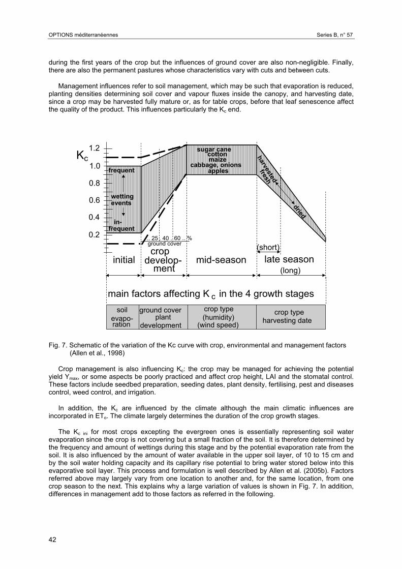
Fig. 7. Schematic of the variation of the Kc curve with crop, environmental and management factors (Allen et al., 1998)

Crop management is also influencing Kc: the crop may be managed for achieving the potential yield Ymax, or some aspects be poorly practiced and affect crop height, LAI and the stomatal control. These factors include seedbed preparation, seeding dates, plant density, fertilising, pest and diseases control, weed control, and irrigation.

In addition, the Kc are influenced by the climate although the main climatic influences are incorporated in ETo. The climate largely determines the duration of the crop growth stages.

The Kc ini for most crops excepting the evergreen ones is essentially representing soil water evaporation since the crop is not covering but a small fraction of the soil. It is therefore determined by the frequency and amount of wettings during this stage and by the potential evaporation rate from the soil. It is also influenced by the amount of water available in the upper soil layer, of 10 to 15 cm and by the soil water holding capacity and its capillary rise potential to bring water stored below into this evaporative soil layer. This process and formulation is well described by Allen et al. (2005b). Factors referred above may largely vary from one location to another and, for the same location, from one crop season to the next. This explains why a large variation of values is shown in Fig. 7. In addition, differences in management add to those factors as referred in the following.

42


The Kc ini may be largely modified by management practices such as direct seeding (no tillage), soil

mulching by straw or plastic, tunneling with plastic as for horticultural crops, and other similar practices. Two effects occur: on the one hand, there is a decrease of energy at the soil surface, thus a decrease of the evaporation rates; on the other hand, there is an increased resistance to vapour transfer from the soil surface into the atmosphere, mainly relative to an increase in the surface resistance. Therefore, Kc ini may be much lower than under conditions when the soil is fully exposed to radiation. However, impacts referred in literature are variable reflecting differences in soil cover; in case of vegetal mulching this highly depend on the amount and distribution of soil coverage; in case of plastic mulch they depend on its transparency to radiation of short and long wave, and on the amount of openings in the plastic through where vapour may escape to the atmosphere. Anyway, in general, soil covering with mulch reduces Kc ini, thus soil evaporation, not affecting transpiration of the canopy. Effects are kept but progressively reduced during the crop development phase and mostly disappear at the mid-season for full cover crops. Adopting the dual crop coefficient approach (Eq. 22) these effects are better studied since it becomes possible to separate the soil evaporation and the transpiration components of ETc

In case of tree and shrub crops where the soil is covered by active vegetation, which is often

required as a measure to combat erosion, the impacts of soil cover are totally different since this vegetation also uses water and the crop water requirements of such crops are then increased relative to bare soil conditions.

The Kc mid essentially varies with the crop but is also affected by the climate, namely when

advective conditions occur. This relation with climate is analysed by Pereira et al. (1999). Therefore, an adjustment to climate is proposed by Allen et al. (1998) aimed at exporting to other climates the tabled values for Kc mid. In fact these tabled values refer to a standard climate where the wind speed u2 is 2 m s-1 and the minimum relative humidity RHmin is 45% during the mid season of the considered crop. Then the adjustment to any other climate is performed through the following equation:

[ ]30

2 34500402040

.

min)climatestandard(midcmidch)RH(.)u(.KK

−−−+= (23)

where Kc mid and Kc mid (standard climate) refer to the location where the application is performed and to the standard conditions, and h is the crop height [m] during mid-season.

This equation shows well the aspects referred above relative to ra since u2 is a main variable controlling ra and determining this equation. he dominant. Kc increases with wind speed and decreases inversely. Therefore, reducing ET at the mid-season may be obtained by avoiding high winds as it is commonly done in arid lands, either through cropping in areas less exposed to wind or using wind breaks. RHmin, for a certain extend, represents well the conditions for diffusion of vapour into the atmosphere, very strong in arid climates where RHmin is low. Changing RH to control evaporation is generally non practical, but RH tends to increase when wind is reduced and thus the transport of vapour from the air layer close to the crop. Eq. 23 shows that these impacts are larger for tall crops and smaller for short ones, which agrees with the above referred increase of ra when the crop is of low height.

The Kc end is largely affected by management which determines harvesting, thus the end of the crop season (Fig. 7). Moreover, harvesting earlier increases Kc end relative to a late harvesting of the same crop but shortens the duration of the end-season period. Harvesting earlier is practiced for food crops that should be eaten fresh, and harvesting later is adopted for crops when conservation or preservation is easier when they are stored dry, as for cereals. Climate also impacts the Kc end when the crop is harvested fresh. Then Eq. 23 applies but variables refer to the the late season. Controlling ET during this period refers to the same aspects as for the mid-season.

Kc values are well known for the temperature climate crops, mainly the annual crops (Allen et al., 1998); some deficiencies in knowledge occur for tree crops due to differences in plant density, ground cover by vegetation or mulch, and architecture of the plantations. However, literature is producing consistent knowledge that provides for adopting coherent values for Kc in other regions. Main gaps

43


refer to tropical and sub-tropical crops, which research is less abundant and largely published in native languages. A great effort in improving the corresponding base-knowledge is necessary.

Frequent gaps in practical knowledge refer to the lack of adoption of appropriate estimation of Kc ini when using the rough indicative values in Tables, and the lack in adjusting the Kc mid and Kc end to climate (Eq. 23). Moreover, it is the use of Kc without referring to the fact that the crop is managed for potential yield or not, thus that crop factor is not differentiate between Kc and Kc act (Eq. 19 and 21). Then is often said that FAO 56 tabled values are not appropriate when the main problem is to use only part of the information produced in the guidelines and omitting the use of all other adjusting tools.

It is necessary to underline herein that looking to develop water productivity assessment without fully considering (and understanding) the concepts and calculation tools for crop evapotranspiration is inadequate since the main component in computing irrigation depths is Etc or ETa and, without knowing these, one can only roughly know how much is the non-beneficial water use term NBWU (Eq. 7 and 11).

WATER STRESS AND IMPACTS ON YIELD

The basic relationship between crop ET and yields may be represented by the Stewart model

(Stewart et al., 1977, Doorenbos and Kassam, 1979) relating the relative yield decrease with the relative evapotranspiration deficit (see Fig. 5)

−=

−

c

actcy

m ETET

KYYa 11 (24)

where Ky is the yield response factor [-], ETcadj is the adjusted (actual) crop evapotranspiration [mm d-

1], ETc is the crop evapotranspiration for standard conditions (no water stress) [mm d-1], Ya is the crop yield when ET = ETcadj , and Ym is the maximal crop yield corresponding to ETc. A better description of ET impacts on yields is obtained when the yield response factors refer to specific crop phases and the history of the crop stresses is taken into consideration as it is largely reported in the literature.

Recombining the terms of Eq. 24, the stress coefficient Ks (Eq. ) may be expressed as

−−=m

a

ys Y

YK

K 111 (25)

which expresses how the relative yield decrease impact the stress coefficient as a function of the yield response factor. However, for operational purposes, it is better to express Ks as a function of the soil water depletion:

−−

=RAWTAWDTAWK r

s (26)

where TAW and RAW are respectively the total and readily available soil water, and Dr is the cumulated soil water depletion between two wetting events by rain or irrigation. Eq. 26 indicates that Ks < 1 when soil water is depleted below the RAW threshold.

Yields may be affected by other environmental and management factors such as salinity (Hamdy and Karajeh, 1999; Minhas, 1996; Rhoades et al., 1992). A simplified approach for salinity impacts for conditions where ECe > ECe threshold is

( )100

1 bECECYY

thresholdeem

a −−= (27)

44


where Ya is the actual crop yield, Ym is the maximum expected crop yield when ECe < ECe threshold, ECe is the mean electrical conductivity of the saturation extract for the root zone [dS m-1], ECe threshold is the electrical conductivity of the saturation extract at the threshold of ECe when crop yield first reduces below Ym [dS m-1], and b is the reduction in yield per increase in ECe [%/(dS m-1)]. Values for ECe threshold and b are tabled by Rhoades et al. (1992) and Allen et al. (1998).

The combined impacts of water and salinity stress are expressed through

( )

−−

−−=

RAWTAWDTAWECEC

KbK r

thresholdeey

s 1001 (28)

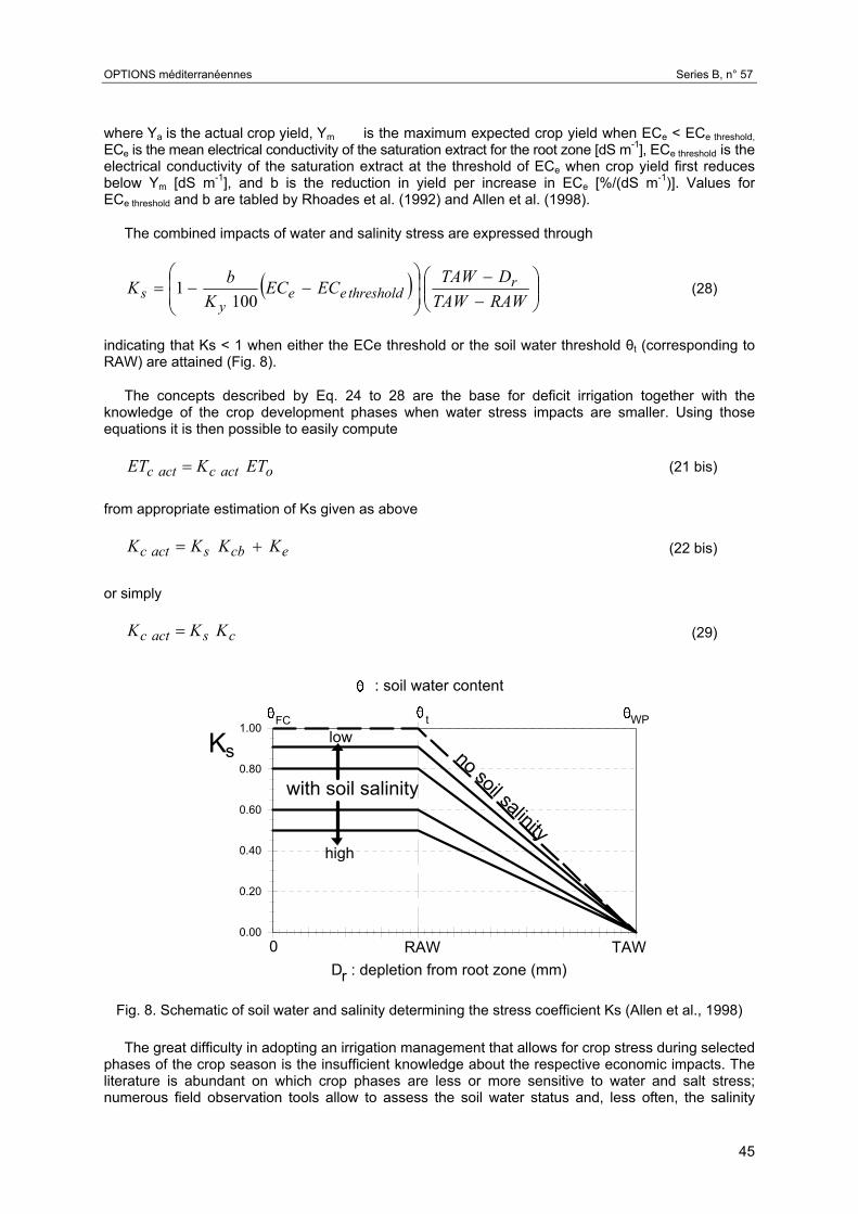
indicating that Ks < 1 when either the ECe threshold or the soil water threshold θt (corresponding to RAW) are attained (Fig. 8).

The concepts described by Eq. 24 to 28 are the base for deficit irrigation together with the knowledge of the crop development phases when water stress impacts are smaller. Using those equations it is then possible to easily compute

oactcactc ETKET = (21 bis)

from appropriate estimation of Ks given as above

ecbsactc KKKK += (22 bis)

or simply

csactc KKK = (29)

0.00

0.20

0.40

0.60

0.80

1.00

: soil water content

FC t W

D : depletion from root zone (mm)r

Ks

0

P

RAW TAW

low

high

with soil salinity

no soil salinity

Fig. 8. Schematic of soil water and salinity determining the stress coefficient Ks (Allen et al., 1998) The great difficulty in adopting an irrigation management that allows for crop stress during selected

phases of the crop season is the insufficient knowledge about the respective economic impacts. The literature is abundant on which crop phases are less or more sensitive to water and salt stress; numerous field observation tools allow to assess the soil water status and, less often, the salinity

45


conditions; a variety of models may be used to simulate the soil water balance and therefore provide appropriate information for irrigation scheduling. Although a few tentative exist (Victoria et al., 2005), the great gap refers to combining physical assessment and simulation with economic assessment of impacts.

In an example referring to Tunisia and Portugal (Rodrigues et al., 2003; Zairi et al., 2003) it is

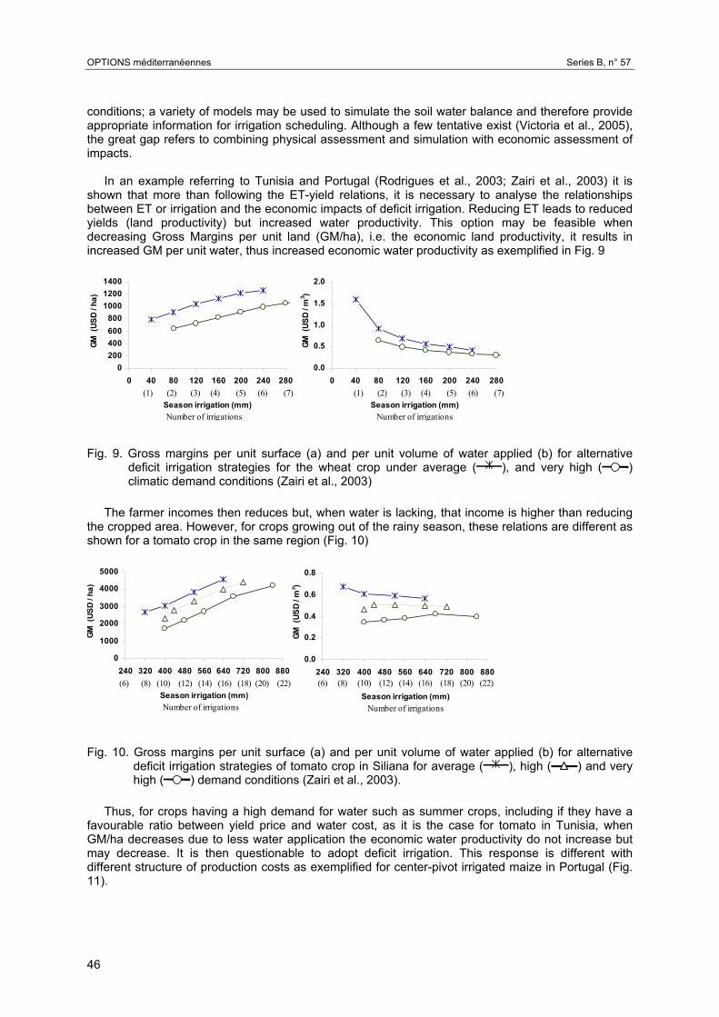
shown that more than following the ET-yield relations, it is necessary to analyse the relationships between ET or irrigation and the economic impacts of deficit irrigation. Reducing ET leads to reduced yields (land productivity) but increased water productivity. This option may be feasible when decreasing Gross Margins per unit land (GM/ha), i.e. the economic land productivity, it results in increased GM per unit water, thus increased economic water productivity as exemplified in Fig. 9

0200400600800

100012001400

0 4

GM (

USD

/ ha)

(1)

2.0

Fig. 9. Grosdeficclima

The farm

the croppedshown for a

0

1000

2000

3000

4000

5000

240 320

GM (

USD

/ ha)

(6) (8)

Fig. 10. Grodefihigh

Thus, for

favourable rGM/ha decrmay decreadifferent stru11).

46

0 80 120 160 200 240 280

Season irrigation (mm) (2) (3) (4) (5) (6) (7)

Number of irrigations

0.0

0.5

1.0

1.5

0 4

GM (

USD

/ m3 )

s margins per unit surface (a) and pit irrigation strategies for the wheat tic demand conditions (Zairi et al., 20

er incomes then reduces but, when w area. However, for crops growing outtomato crop in the same region (Fig. 1

400 480 560 640 720 800 880

Season irrigation (mm) (10) (12) (14) (16) (18) (20) (22)


0.0

0.2

0.4

0.6

0.8

240 320

GM (

USD

/ m3 )

(6) (8)

ss margins per unit surface (a) and cit irrigation strategies of tomato crop ( ) demand conditions (Zairi et a

crops having a high demand for waatio between yield price and water ceases due to less water application tse. It is then questionable to adopcture of production costs as exempli

0 80 120 160 200 240 280

Season irrigation (mm)(1) (2) (3) (4) (5) (6) (7)


er unit volume of water applied (b) for alternative crop under average ( ), and very high ( ) 03)

ater is lacking, that income is higher than reducing of the rainy season, these relations are different as 0)

400 480 560 640 720 800 880

Season irrigation (mm) (10) (12) (14) (16) (18) (20) (22)


per unit volume of water applied (b) for alternative in Siliana for average ( ), high ( ) and very l., 2003).

ter such as summer crops, including if they have a ost, as it is the case for tomato in Tunisia, when

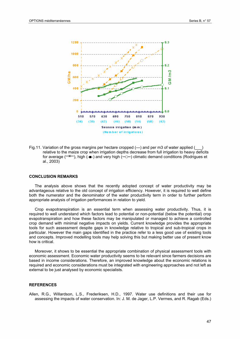
he economic water productivity do not increase but t deficit irrigation. This response is different with fied for center-pivot irrigated maize in Portugal (Fig.


Fig.11. Variation of the gross margins per hectare cropped (---) and per m3 of water applied (___) relative to the maize crop when irrigation depths decrease from full irrigation to heavy deficits for average ( ), high ( ) and very high ( ) climatic demand conditions (Rodrigues et al., 2003)

CONCLUSION REMARKS

The analysis above shows that the recently adopted concept of water productivity may be advantageous relative to the old concept of irrigation efficiency. However, it is required to well define both the numerator and the denominator of the water productivity term in order to further perform appropriate analysis of irrigation performances in relation to yield.

Crop evapotranspiration is an essential term when assessing water productivity. Thus, it is required to well understand which factors lead to potential or non-potential (below the potential) crop evapotranspiration and how these factors may be manipulated or managed to achieve a controlled crop demand with minimal negative impacts on yields. Current knowledge provides the appropriate tools for such assessment despite gaps in knowledge relative to tropical and sub-tropical crops in particular. However the main gaps identified in the practice refer to a less good use of existing tools and concepts. Improved modelling tools may help solving this but making better use of present know how is critical.

Moreover, it shows to be essential the appropriate combination of physical assessment tools with economic assessment. Economic water productivity seems to be relevant since farmers decisions are based in income considerations. Therefore, an improved knowledge about the economic relations is required and economic considerations must be integrated with engineering approaches and not left as external to be just analysed by economic specialists.

REFERENCES Allen, R.G., Willardson, L.S., Frederiksen, H.D., 1997. Water use definitions and their use for

assessing the impacts of water conservation. In: J. M. de Jager, L.P. Vermes, and R. Ragab (Eds.)

47


Sustainable Irrigation in Areas of Water Scarcity and Drought (Proc. ICID Workshop, Oxford), British Nat. Com. ICID, Oxford, pp. 72-81.

Allen, R.G., Smith, M., Perrier, A., Pereira, L.S., 1994. An update for the definition of reference evapotranspiration. ICID Bulletin, 43(2): 1-34.

Allen, R.G., Pereira, L.S., Raes, D., Smith, M., 1998. Crop Evapotranspiration. Guidelines for Computing Crop Water Requirements. FAO Irrig. Drain. Paper 56, FAO, Rome, 300 p.

Allen, R.G., Pereira, L.S., Smith, M., Raes, D., Wright, J.L., 2005a. FAO-56 Dual crop coefficient method for estimating evaporation from soil and application extensions. J. Irrig. Drain. Engng. 131(1): 2-13.

Allen, R.G., Pruitt, W.O., Raes, D., Smith, M., Pereira, L.S., 2005b. Estimating evaporation from bare soil and the crop coefficient for the initial period using common soils information. J. Irrig. Drain. Engng. 131(1): 14-23.

Alves, I, Pereira, L.S., 2000. Modelling surface resistance from climatic variables? Agric. Water Manag. 42: 371-385.

Alves, I., Perrier, A., Pereira, L.S., 1998. Aerodynamic and surface resistances of complete cover crops: How good is the “big leaf” approach? Trans. ASAE 41(2): 345-351.

Baldocchi, D.D., Luxmoore, R.J., Hatfield, J.L., 1991. Discerning the forest from the trees: an essay on scaling canopy stomatal conductance. Agric. For. Meteorol. 54: 197-226.

Bos, M.G., Burton, M.A., Molden, D.J., 2005. Irrigation and drainage Performance Assessment. Practical Guidelines. CABI Publ. Wallingford.

Brutsaert, W., 1982. Evaporation into the Atmosphere. R. Deidel Publ. Co, Dordrecht, Burt, C.M., Clemmens, A.J., Strelkoff, T.S., Solomon, K.H., Bliesner, R.D., Hardy, L.A., Howell, T.A.,

Eisenhauer, D.E., 1997. Irrigation performance measures: efficiency and uniformity. J. Irrig. Drain. Engng. 123: 423-442.

FAO, 2002. Crops and drops: making the best use of water for agriculture. FAO, Land and Water Development Division, Rome, Italy

Hamdy, A., Karajeh, F., (Eds.) 1999. Marginal Water Management for Sustainable Agriculture in Dry Areas. (Proc. Advanced Short Course, Aleppo, Syria), ICARDA, Aleppo and CIHEAM/IAM-B, Istituto Agronomico Mediterraneo, Bari.

Jensen, M.E., 1996. Irrigated agriculture at the crossroads. In: Pereira, L. S., Feddes, R. A., Gilley, J. R., Lesaffre, B. (Eds.) Sustainability of Irrigated Agriculture. Kluwer Acad. Publ., Dordrecht, pp. 19-33.

Jensen, M.E., Burman, R.D., Allen, R.G. (Eds.), 1990. Evapotranspiration and Irrigation Water Requirements. Am. Soc. Civ. Eng. Manual No. 70, 332 pp.

Keller, J., Bliesner, R.D., 1990. Sprinkler and Trickle Irrigation. Van Nostrand Reinhold, New York, 652 pp.

Lamaddalena, N., Pereira, L.S., 1998. Performance analysis of on-demand pressurized irrigation systems. In: Pereira, L.S., Gowing, J.W. (Eds.) Water and the Environment: Innovation Issues in Irrigation and Drainage, E &FN Spon, London, pp. 247-255.

Lamaddalena, N., Sagardoy, J.A., 2000. Performance Analysis of On-Demand Pressurized Irrigation Systems. FAO Irrigation and Drainage Paper 59, FAO, Rome, 132 pp.

Mantovani, E.C., Villalobos, F.J., Orgaz, F., Fereres, E., 1995. Modelling the effects of sprinkler irrigation uniformity on crop yield. Agric. Water Manage. 27: 243-257.

Minhas, P.S., 1996. Saline water management for irrigation in India. Agric. Water Manage. 38: 1-24. Molden, D.J. and Gates, T.K., 1990. Performance measures for evaluation of irrigation-water-delivery

systems. J. Irrigation and Drainage Engineering 116(6): 804-823. Molden, D., Murray-Rust, H., Sakthivadivel, R., Makin, I., 2003. A water-productivity framework for

understanding and action. In: Kijne JW, Barker R, Molden D (eds.), Water Productivity in Agriculture: Limits and Opportunities for Improvement, IWMI and CABI Publ., Wallingford, pp 1-18.

Monteith, J.L., 1965. Evaporation and the environment. XIXth Symposia of the Society for Experimental Biology. In the State and Movement of Water in Living Organisms. University Press, Swansea, Cambridge, 205–234.

Monteith, J.L. 1973. Principles of Environmental Physics. Edward Arnold, London.

48


Ortega, J.F., de Juan, J.A., Tarjuelo, J.M., 2005. Improving Water Management: The Irrigation

Advisory Service of Castilla la Mancha (Spain). Agric. Water Manage. 77: 37-58. Pereira, L.S., 1999. Higher performances through combined improvements in irrigation methods and

scheduling: a discussion. Agric. Water Manage. 40 (2): 153-169. Pereira, L.S., 2003. Performance issues and challenges for improving water use and productivity

(Keynote). In: T. Hata and A H Abdelhadi (Session Organizers) Participatory Management of Irrigation Systems, Water Utilization Techniques and Hydrology (Proc. Int. Workshop, The 3rd World Water Forum, Kyoto), Water Environment Lab., Kobe University, pp. 1-17.

Pereira, L.S., Trout, T.J., 1999. Irrigation methods. In: van Lier, H.N., Pereira, L.S., Steiner, F.R. (Eds.) CIGR Handbook of Agricultural Engineering, vol. I: Land and Water Engineering, ASAE, St. Joseph, MI, pp. 297-379.

Pereira, L.S., Perrier, A., Allen, R.G., Alves, I., 1999. Evapotranspiration: Review of concepts and future trends. J. Irrig. Drain. Engng. 125(2): 45-51.

Pereira, L.S., Cordery, I., Iacovides, I., 2002a. Coping with Water Scarcity. UNESCO IHP VI, Technical Documents in Hydrology No. 58, UNESCO, Paris, 267 p. (accessible through http://unesdoc.unesco.org/images/0012/001278/127846e.pdf)

Pereira, L.S., Oweis, T., Zairi, A., 2002b. Irrigation management under water scarcity. Agric. Water Manag. 57: 175-206.

Pereira, L.S., Calejo, M.J., Lamaddalena, N., Douieb, A., Bounoua, R., 2003. Design and performance analysis of low pressure irrigation distribution systems. Irrigation and Drainage Systems 17(4): 305-324.

Perrier, A., 1975. Etude physique de l'évapotranspiration dans les conditions naturelles. III - évapotranspiration réelle et potentielle des couverts végétaux. Ann. Agronomiques 26: 229-243.

Perrier, A., 1982. Land surface processes: vegetation. In: Eagleson, P.S. (ed) - Land Surface Processes in Atmospheric General Circulation Models, Cambridge Univ. Press, Cambridge, Mass., pp 395 - 448.

Rhoades, J.D., Kandiah, A., Mashali, A.M., 1992. The Use of Saline Waters for Crop Production. FAO Irrigation and Drainage Paper 48, FAO, Rome.

Rochette, P.; Pattey, E.; Desjardins, R.L.; Dwyer, L.M.; Stewart, D.W.; Dube, P.A., 1991. Estimation of maize (Zea mays L.) canopy conductance by scaling up leaf stomatal conductance. Agric. For. Meteorol. 54: 241-261.

Rodrigues, P.N., T. Machado, L.S. Pereira, J.L. Teixeira, H. El Amami, A. Zairi, 2003. Feasibility of deficit irrigation with center-pivot to cope with limited water supplies in Alentejo, Portugal. In: G. Rossi, A. Cancelliere, L. S. Pereira, T. Oweis, M. Shatanawi, A. Zairi (Eds.) Tools for Drought Mitigation in Mediterranean Regions. Kluwer, Dordrecht, pp. 203-222.

Rossi, G., Cancellieri, A., Pereira, L.S., Oweis, T., Shatanawi, M., Zairi, A. (eds.), 2003. Tools for Drought Mitigation in Mediterranean Regions. Kluwer, Dordrecht, 357 p.

Steduto, P., 1996. Water use efficiency. In: Pereira, L. S., Feddes, R. A., Gilley, J. R., Lesaffre, B. (Eds.) Sustainability of Irrigated Agriculture. Kluwer, Dordrecht, pp. 193-209.

Stockle, C.O.; Kjelgaard, J., 1996. Parameterizing Penman-Monteith surface resistance for estimating daily crop ET. In: Camp, C.R.; Sadler, E.J.; Yoder, R.E. (eds) Evapotranspiration and Irrigation Scheduling (Proc. Int. Conf., San Antonio, Texas, 3-6 Nov), ASAE, St. Joseph, MI, pp. 697-703.

Victoria F.B., Viegas Filho J.S., Pereira L.S., Teixeira J.L., Lanna A.E., 2005. Multi-scale modeling for water resources planning and management in rural basins. Agric. Water Manage. 77: 4-20.

Zairi, A., H. El Amami, A. Slatni, L.S. Pereira, P.N. Rodrigues, T. Machado, 2003. Coping with drought: deficit irrigation strategies for cereals and field horticultural crops in Central Tunisia. In: G. Rossi, A. Cancelliere, L. S. Pereira, T. Oweis, M. Shatanawi, A. Zairi (Eds.) Tools for Drought Mitigation in Mediterranean Regions. Kluwer, Dordrecht, pp. 181-201.

Zhang, H., Oweis, T., 1999. Water-yield relations and optimal irrigation scheduling of wheat in the Mediterranean region. Agric. Water Manag. 38: 195-211.

49